Download OS-9 BASIC User Manual

OS-9 BASIC
User Manual
Copyright and Revision
History
Copyright  1991 Microware Systems Corporation. All Rights Reserved.
Reproduction of this document, in part or whole, by any means, electrical,
mechanical, magnetic, optical, chemical, manual or otherwise is prohibited, without written permission from Microware Systems Corporation.
This manual reflects Version 2.4 of Microware BASIC. Version 2.4 of
Microware BASIC is to be used with Version 2.4 or greater of the OS-9
operating system.
Revision
Publication Date:
Publication Editor:
Product Number:
G
January, 1991
Walden Miller, Ellen Grant
BAS-68-NA-68-MO
Disclaimer
The information contained herein is believed to be accurate as of the date
of publication. However, Microware will not be liable for any damages,
including indirect or consequential, from use of the OS-9 operating system,
Microware-provided software or reliance on the accuracy of this
documentation. The information contained herein is subject to change
without notice.
Reproduction Notice
The software described in this document is intended to be used on a single
computer system. Microware expressly prohibits any reproduction of the
software on tape, disk or any other medium except for backup purposes.
Distribution of this software, in part or whole, to any other party or on any
other system may constitute copyright infringements and misappropriation
of trade secrets and confidential processes which are the property of
Microware and/or other parties. Unauthorized distribution of software may
cause damages far in excess of the value of the copies involved.
For additional copies of this software and/or documentation, or if you have
questions concerning the above notice, the documentation and/or software,
please contact your OS-9 supplier.
Trademarks
OS-9, Personal OS-9, Professional OS-9, Basic09, and Microware Basic
are trademarks of Microware Systems Corp.
UNIX is a trademark of Bell Laboratories.
Microware Systems Corporation • 1900 N.W. 114th Street
Des Moines, Iowa 50325-7077 • Phone: 515/224-1929
Preface
Introduction
Introduction
Microware BASIC is an enhanced structured Basic language programming
system. It was created for the 68000 Microprocessor.
In addition to the standard BASIC language statements and functions,
Microware BASIC includes many of the useful elements of the PASCAL
programming language. This allows programs to be modular,
well-structured, and use sophisticated data structures. It permits full access
to almost all of the OS-9 operating system commands and functions so it
can be used as a systems programming language.
Microware BASIC is unusual in that it is an interactive compiler. It has
the fast execution speed typical of compiler languages and the ease of use
and memory space efficiency typical of interpreter languages.
Microware BASIC includes a powerful text editor, a multi-pass compiler, a
run-time interpreter, a high-level interactive debugger, and a system
executive. Each of these components is carefully integrated so you see a
friendly, highly interactive programming resource. It provides all the tools
and helpful facilities needed for fast, accurate creation and testing of
structured programs.
These features make Microware BASIC an ideal language for many
applications: scientific, business, industrial control, and education.
Microware BASIC Features
Structured, recursive BASIC with Pascal-type enhancements:
allows multiple, independent, named procedures
procedures called by name with parameters
multi-character, upper or lower case identifiers
variables and line numbers local to procedures
line numbers optional
automatic linkage to ROM or RAM “library” procedures
PACK command compacts program and provides security
PRINT USING with FORTRAN-like format specifications
i
Preface
Introduction
Extended Control Structures (with Unique Closure Elements):
IF...THEN...[ ELSE...] ENDIF
FOR...TO...[ STEP ]...NEXT
REPEAT...UNTIL...
WHILE...DO...ENDWHILE
LOOP...ENDLOOP
EXITIF...THEN...ENDEXIT
High-speed, high-accuracy math:
14 decimal-digit 64 bit binary floating point
Full set of transcendentals (SIN, ASN, ACS, LOG, etc.)
Extended data structures:
Five Basic data types: BYTE, INTEGER, REAL, BOOLEAN, and
STRING
One, two, or three dimensional arrays
User-defined complex structures and data types
Powerful interactive debugging and editing features:
Integral, full-featured text editor
Syntax error check upon line entry and procedure compile
Trace mode reproduces original source statements
Renumber command for line numbered procedures
The History of Microware
BASIC
Microware Basic was conceived in 1978 as a high-performance
programming language to demonstrate the capabilities of the 6809
microprocessor to efficiently run high-level languages. Microware BASIC
was developed at the same time as the 6809 under the auspices of the
architects of the 6809. It was originally titled Basic09. The project covered
almost two years, and incorporated the results of research in such areas as
interactive compilation, fast floating point arithmetic algorithms, storage
management, high-level symbolic debugging, and structured language
design. These innovations give Microware BASIC its speed, power, and
unique flavor.
Microware BASIC was commissioned by Motorola, Inc., Austin, Texas,
and developed by Microware Systems Corporation, Des Moines, Iowa.
Principal designers of Microware BASIC were Larry Crane, Robert
Doggett, Ken Kaplan, and Terry Ritter. The first release was in February,
1980.
Excellent feedback, thoughtful suggestions, and carefully documented bug
reports from Microware BASIC users all over the world have been
invaluable to the designers in their efforts to achieve the degree of
sophistication and reliability Microware BASIC has today.
ii
Preface
Introduction
Concerning This Manual
This manual is divided into two parts: the BASIC Tutorial and the BASIC
Reference Manual.
The tutorial section is written for beginning programmers having little
experience with Pascal or other high level languages. Beginning
programmers should work through the examples given to help familiarize
themselves with Microware BASIC control structure.
Readers having adequate programming skills are urged to browse the
tutorial for a feeling of the Microware BASIC environment. A complete
index is provided for easy use of the reference section.
In this manual, Microware BASIC is referred to as BASIC, unless making
reference to other BASIC languages.
iii
Table of Contents
OS-9 BASIC User Manual
SECTION 1
THE BASIC TUTORIAL
Overview
Chapter 1
Introduction . . . . . . . . . . . . . . . . . . . . . . . . . . . . . . . . . . . . . . . . . . . . . . . .
Getting Started . . . . . . . . . . . . . . . . . . . . . . . . . . . . . . . . . . . . . . . . . . . . . .
Fundamental Commands . . . . . . . . . . . . . . . . . . . . . . . . . . . . . . . . . . . . . .
Getting Started
1-1
1-1
1-2
Chapter 2
Naming Your Procedure . . . . . . . . . . . . . . . . . . . . . . . . . . . . . . . . . . . . . .
Writing Your First Procedure . . . . . . . . . . . . . . . . . . . . . . . . . . . . . . . . . .
The DIM Statement: Declaring Variables . . . . . . . . . . . . . . . . . . . . . . . . .
Variable Data Types . . . . . . . . . . . . . . . . . . . . . . . . . . . . . . . . . . . . . . . . . .
Constants . . . . . . . . . . . . . . . . . . . . . . . . . . . . . . . . . . . . . . . . . . . . . . . . . .
Operators . . . . . . . . . . . . . . . . . . . . . . . . . . . . . . . . . . . . . . . . . . . . . . . . . .
Conditional Control: The IF..THEN Structure . . . . . . . . . . . . . . . . . . . . .
Looping Statements . . . . . . . . . . . . . . . . . . . . . . . . . . . . . . . . . . . . . . . . . .
Editing Your Procedures . . . . . . . . . . . . . . . . . . . . . . . . . . . . . . . . . . . . . .
Line Numbers and the GOTO Statement . . . . . . . . . . . . . . . . . . . . . . . . .
Putting It All Together . . . . . . . . . . . . . . . . . . . . . . . . . . . . . . . . . . . . . . . .
Program Construction:
Complex Data Types and
Subroutines
Chapter 3
Program Optimization
Chapter 4
Introduction . . . . . . . . . . . . . . . . . . . . . . . . . . . . . . . . . . . . . . . . . . . . . . . .
Arrays . . . . . . . . . . . . . . . . . . . . . . . . . . . . . . . . . . . . . . . . . . . . . . . . . . . .
The TYPE Declaration . . . . . . . . . . . . . . . . . . . . . . . . . . . . . . . . . . . . . . .
External Files . . . . . . . . . . . . . . . . . . . . . . . . . . . . . . . . . . . . . . . . . . . . . . .
Subroutines . . . . . . . . . . . . . . . . . . . . . . . . . . . . . . . . . . . . . . . . . . . . . . . .
Calling Procedures . . . . . . . . . . . . . . . . . . . . . . . . . . . . . . . . . . . . . . . . . . .
Command Line Parameters . . . . . . . . . . . . . . . . . . . . . . . . . . . . . . . . . . . .
Formatted Output: The PRINT .. USING Statement . . . . . . . . . . . . . . . .
General Execution Performance of BASIC . . . . . . . . . . . . . . . . . . . . . . . .
Optimum Use of Numeric Data Types . . . . . . . . . . . . . . . . . . . . . . . . . . .
Looping Quickly . . . . . . . . . . . . . . . . . . . . . . . . . . . . . . . . . . . . . . . . . . . .
Optimum Use of Arrays and Data Structures . . . . . . . . . . . . . . . . . . . . . .
The PACK Command . . . . . . . . . . . . . . . . . . . . . . . . . . . . . . . . . . . . . . . .
Eliminating Constant Expressions and Sub-Expressions . . . . . . . . . . . . .
Fast Input and Output Functions . . . . . . . . . . . . . . . . . . . . . . . . . . . . . . . .
Professional Programming Techniques . . . . . . . . . . . . . . . . . . . . . . . . . . .
2-1
2-2
2-4
2-8
2-8
2-10
2-12
2-13
2-18
2-24
2-25
3-1
3-1
3-4
3-4
3-10
3-12
3-14
3-17
4-1
4-2
4-2
4-3
4-3
4-3
4-3
4-4
I
Table of Contents
OS-9 BASIC User Manual
SECTION 2
BASIC REFERENCE GUIDE
System Mode
Chapter 5
System Mode Commands . . . . . . . . . . . . . . . . . . . . . . . . . . . . . . . . . . . . .
$ .........................................................
BYE (or <eof> character) . . . . . . . . . . . . . . . . . . . . . . . . . . . . . . . . . . . . .
CHD/CHX . . . . . . . . . . . . . . . . . . . . . . . . . . . . . . . . . . . . . . . . . . . . . . . . .
DIGITS . . . . . . . . . . . . . . . . . . . . . . . . . . . . . . . . . . . . . . . . . . . . . . . . . . .
DIR . . . . . . . . . . . . . . . . . . . . . . . . . . . . . . . . . . . . . . . . . . . . . . . . . . . . . .
EDIT/E . . . . . . . . . . . . . . . . . . . . . . . . . . . . . . . . . . . . . . . . . . . . . . . . . . .
KILL/KILL* . . . . . . . . . . . . . . . . . . . . . . . . . . . . . . . . . . . . . . . . . . . . . . .
LIST/LIST* . . . . . . . . . . . . . . . . . . . . . . . . . . . . . . . . . . . . . . . . . . . . . . . .
LOAD . . . . . . . . . . . . . . . . . . . . . . . . . . . . . . . . . . . . . . . . . . . . . . . . . . . .
MEM . . . . . . . . . . . . . . . . . . . . . . . . . . . . . . . . . . . . . . . . . . . . . . . . . . . . .
PACK/PACK* . . . . . . . . . . . . . . . . . . . . . . . . . . . . . . . . . . . . . . . . . . . . . .
RENAME . . . . . . . . . . . . . . . . . . . . . . . . . . . . . . . . . . . . . . . . . . . . . . . . .
RUN . . . . . . . . . . . . . . . . . . . . . . . . . . . . . . . . . . . . . . . . . . . . . . . . . . . . . .
SAVE/SAVE* . . . . . . . . . . . . . . . . . . . . . . . . . . . . . . . . . . . . . . . . . . . . . .
Edit Mode
Chapter 6
Edit Mode Commands . . . . . . . . . . . . . . . . . . . . . . . . . . . . . . . . . . . . . . . .
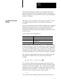
How the Editor Works . . . . . . . . . . . . . . . . . . . . . . . . . . . . . . . . . . . . . . . .
Line-Number Oriented Editing . . . . . . . . . . . . . . . . . . . . . . . . . . . . . . . . .
String-Oriented Editing . . . . . . . . . . . . . . . . . . . . . . . . . . . . . . . . . . . . . . .
Execution Mode
6-1
6-2
6-3
6-4
Chapter 7
Running Programs . . . . . . . . . . . . . . . . . . . . . . . . . . . . . . . . . . . . . . . . . . .
Execution Mode: Technically Speaking . . . . . . . . . . . . . . . . . . . . . . . . . .
II
5-1
5-3
5-4
5-4
5-5
5-5
5-6
5-6
5-7
5-7
5-8
5-8
5-9
5-10
5-10
7-1
7-2
Table of Contents
OS-9 BASIC User Manual
Debug Mode
Chapter 8
Overview of Debug Mode . . . . . . . . . . . . . . . . . . . . . . . . . . . . . . . . . . . . .
$ .........................................................
BREAK . . . . . . . . . . . . . . . . . . . . . . . . . . . . . . . . . . . . . . . . . . . . . . . . . . .
CONT . . . . . . . . . . . . . . . . . . . . . . . . . . . . . . . . . . . . . . . . . . . . . . . . . . . .
DEG/RAD . . . . . . . . . . . . . . . . . . . . . . . . . . . . . . . . . . . . . . . . . . . . . . . . .
DIR . . . . . . . . . . . . . . . . . . . . . . . . . . . . . . . . . . . . . . . . . . . . . . . . . . . . . .
LET . . . . . . . . . . . . . . . . . . . . . . . . . . . . . . . . . . . . . . . . . . . . . . . . . . . . . .
LIST . . . . . . . . . . . . . . . . . . . . . . . . . . . . . . . . . . . . . . . . . . . . . . . . . . . . . .
PRINT . . . . . . . . . . . . . . . . . . . . . . . . . . . . . . . . . . . . . . . . . . . . . . . . . . . .
Q ........................................................
STATE . . . . . . . . . . . . . . . . . . . . . . . . . . . . . . . . . . . . . . . . . . . . . . . . . . . .
STEP . . . . . . . . . . . . . . . . . . . . . . . . . . . . . . . . . . . . . . . . . . . . . . . . . . . . .
TRON/TROFF . . . . . . . . . . . . . . . . . . . . . . . . . . . . . . . . . . . . . . . . . . . . . .
Debugging Techniques . . . . . . . . . . . . . . . . . . . . . . . . . . . . . . . . . . . . . . .
Debug Mode as a Desk Calculator . . . . . . . . . . . . . . . . . . . . . . . . . . . . . .
Data Types and Data
Structures
8-1
8-2
8-2
8-3
8-3
8-4
8-4
8-4
8-5
8-5
8-5
8-6
8-6
8-7
8-8
Chapter 9
Data Types . . . . . . . . . . . . . . . . . . . . . . . . . . . . . . . . . . . . . . . . . . . . . . . . .
Data Structures . . . . . . . . . . . . . . . . . . . . . . . . . . . . . . . . . . . . . . . . . . . . .
The Five Basic Data Types . . . . . . . . . . . . . . . . . . . . . . . . . . . . . . . . . . . .
The BYTE Data Type . . . . . . . . . . . . . . . . . . . . . . . . . . . . . . . . . . . . . . . .
The INTEGER Data Type . . . . . . . . . . . . . . . . . . . . . . . . . . . . . . . . . . . . .
The REAL Data Type . . . . . . . . . . . . . . . . . . . . . . . . . . . . . . . . . . . . . . . .
Internal Representation of REAL Numbers . . . . . . . . . . . . . . . . . . . . . . .
The STRING Data Type . . . . . . . . . . . . . . . . . . . . . . . . . . . . . . . . . . . . . .
The BOOLEAN Data Type . . . . . . . . . . . . . . . . . . . . . . . . . . . . . . . . . . . .
Automatic Type Conversion . . . . . . . . . . . . . . . . . . . . . . . . . . . . . . . . . . .
Constants . . . . . . . . . . . . . . . . . . . . . . . . . . . . . . . . . . . . . . . . . . . . . . . . . .
Numeric Constants . . . . . . . . . . . . . . . . . . . . . . . . . . . . . . . . . . . . . . . . . .
Boolean Constants . . . . . . . . . . . . . . . . . . . . . . . . . . . . . . . . . . . . . . . . . . .
String Constants . . . . . . . . . . . . . . . . . . . . . . . . . . . . . . . . . . . . . . . . . . . . .
Variables . . . . . . . . . . . . . . . . . . . . . . . . . . . . . . . . . . . . . . . . . . . . . . . . . .
Parameter Variables . . . . . . . . . . . . . . . . . . . . . . . . . . . . . . . . . . . . . . . . . .
Arrays . . . . . . . . . . . . . . . . . . . . . . . . . . . . . . . . . . . . . . . . . . . . . . . . . . . .
Complex Data Types . . . . . . . . . . . . . . . . . . . . . . . . . . . . . . . . . . . . . . . . .
9-1
9-1
9-2
9-2
9-3
9-3
9-4
9-4
9-5
9-6
9-6
9-6
9-7
9-7
9-7
9-8
9-9
9-9
III
Table of Contents
OS-9 BASIC User Manual
Expressions, Operators, and Chapter 10
Functions
Evaluation of Expressions . . . . . . . . . . . . . . . . . . . . . . . . . . . . . . . . . . . . . 10-1
Operators . . . . . . . . . . . . . . . . . . . . . . . . . . . . . . . . . . . . . . . . . . . . . . . . . .
Operator Precedence . . . . . . . . . . . . . . . . . . . . . . . . . . . . . . . . . . . . . . . . .
Functions . . . . . . . . . . . . . . . . . . . . . . . . . . . . . . . . . . . . . . . . . . . . . . . . . .
Program Statements and
Structure
IV
10-2
10-3
10-4
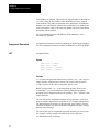
Chapter 11
Program Structure . . . . . . . . . . . . . . . . . . . . . . . . . . . . . . . . . . . . . . . . . . .
Assignment Statements . . . . . . . . . . . . . . . . . . . . . . . . . . . . . . . . . . . . . . .
LET . . . . . . . . . . . . . . . . . . . . . . . . . . . . . . . . . . . . . . . . . . . . . . . . . . . . . .
POKE . . . . . . . . . . . . . . . . . . . . . . . . . . . . . . . . . . . . . . . . . . . . . . . . . . . . .
Control Statements . . . . . . . . . . . . . . . . . . . . . . . . . . . . . . . . . . . . . . . . . .
IF..THEN..ELSE . . . . . . . . . . . . . . . . . . . . . . . . . . . . . . . . . . . . . . . . . . . .
FOR..NEXT . . . . . . . . . . . . . . . . . . . . . . . . . . . . . . . . . . . . . . . . . . . . . . . .
WHILE..DO . . . . . . . . . . . . . . . . . . . . . . . . . . . . . . . . . . . . . . . . . . . . . . .
REPEAT..UNTIL . . . . . . . . . . . . . . . . . . . . . . . . . . . . . . . . . . . . . . . . . . . .
LOOP..ENDLOOP/EXITIF..ENDEXIT . . . . . . . . . . . . . . . . . . . . . . . . . .
GOTO . . . . . . . . . . . . . . . . . . . . . . . . . . . . . . . . . . . . . . . . . . . . . . . . . . . .
GOSUB..RETURN . . . . . . . . . . . . . . . . . . . . . . . . . . . . . . . . . . . . . . . . . .
ON GOTO/ON GOSUB . . . . . . . . . . . . . . . . . . . . . . . . . . . . . . . . . . . . . .
ON ERROR GOTO . . . . . . . . . . . . . . . . . . . . . . . . . . . . . . . . . . . . . . . . . .
Execution Statements . . . . . . . . . . . . . . . . . . . . . . . . . . . . . . . . . . . . . . . .
RUN . . . . . . . . . . . . . . . . . . . . . . . . . . . . . . . . . . . . . . . . . . . . . . . . . . . . . .
KILL . . . . . . . . . . . . . . . . . . . . . . . . . . . . . . . . . . . . . . . . . . . . . . . . . . . . .
CHAIN . . . . . . . . . . . . . . . . . . . . . . . . . . . . . . . . . . . . . . . . . . . . . . . . . . .
SHELL . . . . . . . . . . . . . . . . . . . . . . . . . . . . . . . . . . . . . . . . . . . . . . . . . . . .
END . . . . . . . . . . . . . . . . . . . . . . . . . . . . . . . . . . . . . . . . . . . . . . . . . . . . . .
STOP . . . . . . . . . . . . . . . . . . . . . . . . . . . . . . . . . . . . . . . . . . . . . . . . . . . . .
BYE . . . . . . . . . . . . . . . . . . . . . . . . . . . . . . . . . . . . . . . . . . . . . . . . . . . . . .
DIGITS . . . . . . . . . . . . . . . . . . . . . . . . . . . . . . . . . . . . . . . . . . . . . . . . . . .
ERROR . . . . . . . . . . . . . . . . . . . . . . . . . . . . . . . . . . . . . . . . . . . . . . . . . . .
PAUSE . . . . . . . . . . . . . . . . . . . . . . . . . . . . . . . . . . . . . . . . . . . . . . . . . . . .
CHD/CHX . . . . . . . . . . . . . . . . . . . . . . . . . . . . . . . . . . . . . . . . . . . . . . . . .
DEG/RAD . . . . . . . . . . . . . . . . . . . . . . . . . . . . . . . . . . . . . . . . . . . . . . . . .
BASE0/BASE1 . . . . . . . . . . . . . . . . . . . . . . . . . . . . . . . . . . . . . . . . . . . . .
TRON/TROFF . . . . . . . . . . . . . . . . . . . . . . . . . . . . . . . . . . . . . . . . . . . . . .
Comment Statements . . . . . . . . . . . . . . . . . . . . . . . . . . . . . . . . . . . . . . . . .
REM/(* . . . . . . . . . . . . . . . . . . . . . . . . . . . . . . . . . . . . . . . . . . . . . . . . . . .
Declaration Statements . . . . . . . . . . . . . . . . . . . . . . . . . . . . . . . . . . . . . . .
DIM . . . . . . . . . . . . . . . . . . . . . . . . . . . . . . . . . . . . . . . . . . . . . . . . . . . . . .
PARAM . . . . . . . . . . . . . . . . . . . . . . . . . . . . . . . . . . . . . . . . . . . . . . . . . . .
TYPE . . . . . . . . . . . . . . . . . . . . . . . . . . . . . . . . . . . . . . . . . . . . . . . . . . . . .
11-1
11-2
11-2
11-3
11-4
11-4
11-5
11-7
11-8
11-9
11-10
11-11
11-12
11-13
11-15
11-15
11-18
11-19
11-20
11-21
11-21
11-22
11-22
11-23
11-23
11-24
11-24
11-25
11-25
11-26
11-26
11-27
11-27
11-29
11-30
Table of Contents
OS-9 BASIC User Manual
Files and Unified
Input/Output
Chapter 12
Sample Programs
Appendix A
Quick Reference
Appendix B
Basic Error Codes
Appendix C
RUNB
Appendix D
Files and Unified Input/Output . . . . . . . . . . . . . . . . . . . . . . . . . . . . . . . . .
I/O Paths . . . . . . . . . . . . . . . . . . . . . . . . . . . . . . . . . . . . . . . . . . . . . . . . . .
INPUT . . . . . . . . . . . . . . . . . . . . . . . . . . . . . . . . . . . . . . . . . . . . . . . . . . . .
PRINT . . . . . . . . . . . . . . . . . . . . . . . . . . . . . . . . . . . . . . . . . . . . . . . . . . . .
OPEN . . . . . . . . . . . . . . . . . . . . . . . . . . . . . . . . . . . . . . . . . . . . . . . . . . . . .
CREATE . . . . . . . . . . . . . . . . . . . . . . . . . . . . . . . . . . . . . . . . . . . . . . . . . .
CLOSE . . . . . . . . . . . . . . . . . . . . . . . . . . . . . . . . . . . . . . . . . . . . . . . . . . .
DELETE . . . . . . . . . . . . . . . . . . . . . . . . . . . . . . . . . . . . . . . . . . . . . . . . . .
SEEK . . . . . . . . . . . . . . . . . . . . . . . . . . . . . . . . . . . . . . . . . . . . . . . . . . . . .
READ . . . . . . . . . . . . . . . . . . . . . . . . . . . . . . . . . . . . . . . . . . . . . . . . . . . .
WRITE . . . . . . . . . . . . . . . . . . . . . . . . . . . . . . . . . . . . . . . . . . . . . . . . . . .
GET/PUT . . . . . . . . . . . . . . . . . . . . . . . . . . . . . . . . . . . . . . . . . . . . . . . . . .
DATA/READ/RESTORE . . . . . . . . . . . . . . . . . . . . . . . . . . . . . . . . . . . . .
Formatted Output: The Print Using Statement . . . . . . . . . . . . . . . . . . . . .
Real Format . . . . . . . . . . . . . . . . . . . . . . . . . . . . . . . . . . . . . . . . . . . . . . . .
Exponential Format . . . . . . . . . . . . . . . . . . . . . . . . . . . . . . . . . . . . . . . . . .
Integer Format . . . . . . . . . . . . . . . . . . . . . . . . . . . . . . . . . . . . . . . . . . . . . .
Hexadecimal Format . . . . . . . . . . . . . . . . . . . . . . . . . . . . . . . . . . . . . . . . .
String Format . . . . . . . . . . . . . . . . . . . . . . . . . . . . . . . . . . . . . . . . . . . . . . .
Boolean Format . . . . . . . . . . . . . . . . . . . . . . . . . . . . . . . . . . . . . . . . . . . . .
Control Specifications . . . . . . . . . . . . . . . . . . . . . . . . . . . . . . . . . . . . . . . .
Repeat Groups . . . . . . . . . . . . . . . . . . . . . . . . . . . . . . . . . . . . . . . . . . . . . .
12-1
12-2
12-3
12-4
12-6
12-7
12-8
12-9
12-10
12-11
12-12
12-13
12-16
12-17
12-19
12-20
12-21
12-22
12-23
12-24
12-25
12-25
V
Section
1
The BASIC Tutorial
This section of the manual describes:
how new Microware BASIC users can become comfortable with
programming BASIC
how users get started programming BASIC
complex data types and subroutines that you can use with
Microware BASIC
how to obtain program optimization when executing your procedures
Chapter
1
Overview
Introduction
This manual is designed for two purposes:
to help new Microware BASIC users become comfortable with
programming in BASIC
to serve as a reference for new and existing users
In order to do this, this manual is divided into two sections. The first
section is a user manual that explains how to create a program with BASIC
and how to use BASIC’s functions to make your programs better. The
second section is a reference manual.
Before using Microware BASIC, you should be familiar with OS-9. You
should be familiar with either the Using Personal OS-9 manual or the
Using Professional OS-9 manual. These manuals provide an understanding
of how OS-9 stores files as well as other useful information.
Getting Started
When you start your computer or log in to your account, the OS-9 prompt
is displayed. This manual uses a dollar sign ($) to represent the
OS-9 prompt.
To enter the BASIC environment, type basic at the $ prompt and press the
[Return] key. OS9 responds by printing:
$ basic
Copyright 1984 by Microware.
Reproduced under license
Microware Basic V2.4
Ready
B:
Important: If you are not running version 2.4 of BASIC, the version
number will be different.
1-1
Chapter 1
Overview
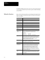
The B: prompt indicates that you are in BASIC’s system mode. Microware
BASIC has four modes:
Mode:
Description:
System Mode
Used for executing system commands.
Edit Mode
Used for creating and editing procedures.
Execution Mode
Used for running procedures.
Debug Mode
Used for testing procedures for errors
You must remember that BASIC does have different modes. You should be
aware that some commands only operate in one mode. Therefore, if you
execute a command that you feel should work and it does not, check that
you are in the proper mode.
These modes are all discussed in more detail in the appropriate sections. A
full description of each mode is located in the reference section of
this manual.
When you create procedures in BASIC, they are created in BASIC’s
workspace. The workspace is the memory area where procedures are
created or loaded, edited, and executed. The procedures in this area are not
automatically saved when you exit BASIC. Therefore, you must save any
files in your workspace before you exit BASIC.
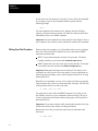
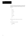
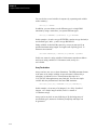
Fundamental Commands
1-2
There are several commands that you should know before beginning to
program in BASIC. These commands are as follows:
Command:
Description:
BYE
Exits BASIC.
DIR
Lists procedures currently in your workspace.
EDIT
Enters edit mode.
KILL
Deletes a procedure from your workspace.
LOAD
Loads files from the OS-9 file system to your workspace.
MEM
Displays or requests workspace memory.
PACK
Compresses a BASIC procedure into BASIC intermediate code.
SAVE
Saves your procedures in the OS-9 file system.
Chapter 1
Overview
BYE: Exiting BASIC
When you have finished using BASIC and have saved all procedures that
you want to save, you can exit BASIC by typing the command BYE at the
system prompt:
B: BYE
You are returned to your OS-9 shell prompt.
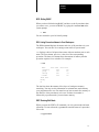
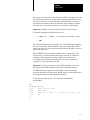
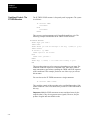
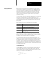
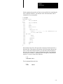
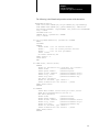
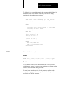
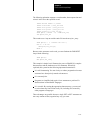
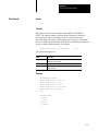
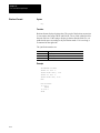
DIR: Listing Procedure Names in Your Workspace
The DIR command displays the names and sizes of all procedures in your
workspace. You can also use a carriage return while in system mode.
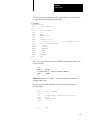
DIR displays a table of all procedure names with two numbers next to each
name. The first column, proc size, is the size of the corresponding
procedure. The data size column shows the amount of memory that the
procedure requires for its variables. For example:
B:DIR
Name
Proc–Size Data–Size
testprog
226
66
prog2
162
82
exloop
220
74
*readit
224
66
4266 free
Ready
B:
The last line shows the amount of free bytes of workspace memory
remaining. You may use this information to estimate how much memory
your program needs to run. You must have at least as much free memory as
the data size of the procedure(s) to be run. If a data size number is
followed by a question mark, you need more memory.
EDIT: Entering Edit Mode
When you enter the EDIT or E command, you exit system mode and enter
edit mode. To enter edit mode, type EDIT or E and the name of a procedure
file to edit:
e myprocedure
1-3
Chapter 1
Overview
If you do not enter a procedure file, BASIC assigns the name Program to
your procedure. The EDIT command is discussed in more detail in the
next chapter.
KILL: Deleting Procedures in Your Workspace
At any time, you may permanently erase one or all of your procedures in
your workspace by using the KILL command. KILL followed by a
procedure name erases the specified procedure. KILL* erases all procedures
in the workspace. For example:
Command:
Description:
B: KILL prog1
Erases prog1 from workspace.
B: KILL*
Erases all procedures from workspace.
LOAD: Loading Procedures
To retrieve a procedure from your current data directory, you can use the
LOAD command followed by the name of the file:
B: LOAD oldprog
This command loads the file oldprog into your workspace. If you have a
procedure in your workspace with the same name as one in the file, BASIC
uses the procedure loaded from the file.
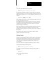
MEM: Displaying or Requesting Workspace Memory
When you enter BASIC, OS-9 automatically allocates approximately 4K of
workspace memory for BASIC. If you need more memory, you can use the
MEM command to get additional memory, if the additional memory is
available. To use the MEM command, type MEM and the amount of memory
you want in bytes. For example:
MEM 20000
This command line requests 20K of memory. BASIC always rounds the
amount you request up to the next highest multiple of 256 bytes. If MEM
displays the following, the requested amount of memory is not available:
What?
1-4
Chapter 1
Overview
You can also use OS-9’s #<memory> option to specify more memory when
you enter BASIC. For example, to call BASIC with 16K of memory, enter
the following command:
$ basic #16k
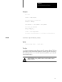
PACK: Compressing Procedures
The PACK command compresses a BASIC procedure and places it in your
current execution directory. Depending on the number of comments, line
numbers, etc., packed procedures execute from 10% to 30% faster than
unpacked procedures. BASIC loads the packed procedure when you try to
run it after it has been packed. The following is an example of
using PACK:
B: PACK exloop
Important: Before you PACK a procedure, always SAVE it first. You
cannot load a packed file into your workspace. Packing a procedure
removes it from your workspace.
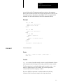
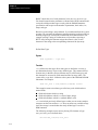
SAVE: Saving Procedures
When you exit BASIC, all unsaved procedures are erased. The SAVE
command allows you to save your programs.
You can use SAVE in a number of ways:
Command:
Description:
Type SAVE by itself.
BASIC creates a file with the name of the last edited or run
procedure in your current data directory. If a file already has this
name, BASIC returns the prompt: Rewrite?. If you respond y for yes,
it replaces the file previously stored in that space with the new
procedure. OS-9 does not allow two files with the same name in the
same directory. By answering n for no, you cancel the SAVE
command without changing the procedure in your workspace or the
file in your directory.
Type SAVE > and a file
name.
This saves the procedure in a file with the specified name.
Type SAVE* and a file
name.
This saves all procedures in your workspace in the specified file.
Type SAVE, followed by This saves the specified procedures in the specified file.
one or more procedures,
followed by a >, followed
by a file name.
Important: If you exit from BASIC, your programs will not automatically
be saved. You must save them using one of these methods or they will
be lost.
1-5
Chapter
2
Getting Started
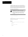
Naming Your Procedure
Programs in BASIC are called procedures. A procedure contains BASIC
instructions as specified by the BASIC language.
Procedures are created in edit mode. To enter edit mode, type e and the
name of the procedure you want to create:
B: e myprogram
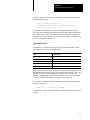
Procedure names may contain from 1 to 28 upper or lower case letters,
numbers, or special characters (as listed below). While the file name may
begin with any of the following characters or digits, the file name must
contain at least one number or letter. Within these limits, a name may
contain any combination of the following:
Description:
Character:
upper case letters
A-Z
underscores
_
lower case letters
a-z
dollar signs
$
numbers
0-9
periods
.
If you do not specify a procedure name, BASIC assigns the name Program
to the new procedure.
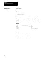
BASIC responds with the following:
B: e myprogram
PROCEDURE myprogram
*
E:
BASIC prints the word PROCEDURE and the name of the procedure. This
is followed by an asterisk (*) signifying the current edit line in the
procedure. The last line displays the edit mode prompt, E:.
2-1
Chapter 2
Getting Started
In edit mode, the first character of each line is reserved for edit commands.
If you forget to type an edit command, BASIC responds with the
following prompt:
What?
The most important edit command is the [Space] character. Placing a
[Space] in the first character position saves the line of the procedure that
immediately follows as a BASIC statement.
Important: The edit commands are discussed later in this chapter. There is
also a chapter in the reference section which deals with the edit commands.
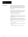
Writing Your First Procedure
When writing your procedure, you will probably want to receive and print
data. You can use the INPUT statement to receive data and the PRINT
statement to print the data.
INPUT accepts data during the execution of a procedure. The data is
normally read from your terminal (the standard input device).
PRINT outputs the text or the values given on the print line. The output
is normally sent to the terminal (the standard output device).
Important: Both input and output can be redirected. This allows you to
read data from a file or print a file to the printer. For more information on
redirecting input and output, refer to either Using Personal OS–9 or Using
Professional OS–9.
With these two commands, you can write a simple procedure, myprogram.
This procedure asks you for your name and prints a message. The first line
of the procedure asks you to enter your name:
E: PRINT “type your name”
You must enter a space before the PRINT statement. If you forget to do
this, BASIC will not save your command. If entered correctly, when you
execute myprogram, the characters between the quotes will be printed on
the terminal screen.
Important: If you make a mistake while entering this procedure line, skip
ahead to the section in this chapter on editing procedures.
Because the user will try to enter their name, the next statement reads
their input:
E: INPUT name$
2-2
Chapter 2
Getting Started
Once again, you must enter a space before the INPUT statement to save the
line. When this procedure is executed, this command causes Basic to wait
for a line of text to be received from the keyboard. BASIC accumulates
text from the keyboard, character by character, until a [Return] ends the
line. This text is saved in the memory reserved for the variable name$.
Important: Variables are discussed in more detail in a later section.
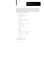
To finish this program, enter the final two lines:
E: PRINT “Hi, ”;name$;“. It’s been nice talking to you.”
*
E: END
The semicolon following the quote after “Hi,” tells BASIC that something
else is to be printed on this line. BASIC inserts the text that the variable
name$ represents. The next semicolon informs BASIC that there is more to
print on the same line.
When a PRINT statement contains multiple values, it prints the values
consecutively. You must separate each of these values by a comma or a
semicolon. If the separator is a comma, BASIC moves to the next
16-column tab stop before printing the next value. If the separator is a
semicolon, no space separates the fields.
Important: If you do not want to use the default tab stops, refer to the
description of the TAB command located in the command summary.
The END statement is optional. It tells BASIC to stop executing the
procedure and return to system mode. BASIC returns to system mode after
executing the last line of code within the procedure.
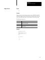
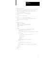
To list your procedure, type l*. This edit mode command lists
the procedure:
E:l*
PROCEDURE myprogram
0000
PRINT “type your name”
0012
INPUT name$
0017
PRINT “Hi, “; name$; ”. It’s been nice talking to you.”
0035
END
*
E:
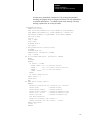
2-3
Chapter 2
Getting Started
Important: The editor has added some information which you did not
type. The numbers to the left of the program are I-code addresses. These
are the actual memory locations where each line begins relative to the start
of the procedure. These numbers may appear strange because they are in
hexadecimal (base 16). The I-code addresses are important because when
BASIC finds an error in a procedure, it conveys as much information as it
has concerning the error. One such piece of information is the I-code
address. Basic automatically supplies I-code addresses.
Now, run the procedure. To run a procedure, you must be in system mode.
You can exit the editor and return to system mode by typing q:
E:q
READY
B:
Now type run myprogram or run. If you enter the RUN command without
a procedure name, BASIC executes the last edited procedure.
B: RUN myprogram
type your name
? Ellen
Hi, Ellen. It’s been nice talking to you.
READY
B:
Important: The question mark (?) prompt tells you that the program is
waiting for input.
Congratulations! You have just written and executed your first program
with Microware BASIC.
The DIM Statement:
Declaring Variables
Procedures use variables to hold values during the execution of the
procedure. The value of a variable may change during execution. In the
example myprogram, name$ was used as a variable to hold the value Ellen.
There are two ways of declaring a variable:
the DIM statement
inferred declaration
The DIM statement declares the variable name and the type of data that is
assigned to it during the course of the procedure. The DIM statement must
occur before you use the variable in the program. This prevents a variable
from being defined with a default data type (inferred declaration). By
standard convention, the DIM statement is used in the first few lines of
a procedure.
2-4
Chapter 2
Getting Started
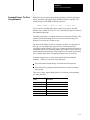
The syntax for the DIM statement is as follows:
DIM <variable>[, <variable>] : <data type>
If you declare more than one variable as the same data type, separate the
variables with commas. If you declare more than one data type in the same
DIM statement, separate the <var>:<type> statements with semicolons. For
example:
DIM x,y,z: INTEGER; a,b,c: REAL
In this example, the variables x, y, and z are defined as integer values, and
a, b, and c are defined as real values.
If the DIM statement is not used and variables are present in a procedure,
the variables are declared with default data types. All undeclared string
variables must end in a dollar sign ($). These variables are assigned a
maximum length of 32 characters.
In the case of name$ in the example myprogram, name$ was declared as a
string variable with a length of 32 characters. If the character string
assigned to name$ is longer than 32 characters, only the first 32 characters
are accepted.
By default, all other variables used are declared as REAL numbers
regardless of the intent of the procedure.
Initializing Variables
Generally, you must initialize variables. BASIC assigns a certain space in
memory large enough to hold the declared type of data. Consequently, if
the variables are not initialized, the variable may contain just about any
value. This makes any operation depending on these variables to be
very unreliable.
You can use either of two assignment statements to initialize variables.
The LET statement has the following syntax:
LET <variable> := <value or constant>
For example, if you have the following command in your procedure, x
equals one:
LET x:=1
You could also enter the following:
LET x=1
2-5
Chapter 2
Getting Started
You can also use an implied statement. Implied statements have the
following syntax:
<variable> := <value or constant>
For example, if you have the following command in your procedure, y
equals ten:
y := 10
You could also enter the following:
y = 10
Naming Variables: Reserved Words
Variable names may be of any length, but you will probably want to keep
them short. This_is_a_legal_variable is legal, but tedious to type. Variable
names must conform to the following rules:
Names must begin with either an underscore or letter.
Names cannot contain embedded blanks or dollar signs.
Names can end in a dollar sign.
Names can contain any alphanumeric or underscores.
Names may not be any BASIC reserved word.
2-6
Chapter 2
Getting Started
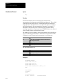
BASIC recognizes certain words as reserved. They cannot be used as
variable names. These reserved words are all commands and key words
used within BASIC statements:
Table 2.A
BASIC Reserved Words
ABS
ACS
ADDR
AND
ASC
ASN
ATN
BASE
BOOLEAN
BYE
BYTE
CHAIN
CHD
CHR$
CHX
CLOSE
COS
CREATE
DATA
DATE$
DEG
DELETE
DIM
DIGITS
DIR
DO
ELSE
END
ENDEXIT
ENDIF
ENDLOOP
ENDWHILE
EOF
ERR
ERROR
EXEC
EXITIF
EXP
FALSE
FILSIZ
FIX
FLOAT
FOR
GET
GOSUB
GOTO
IF
INKEY
INPUT
INT
INTEGER
KILL
LAND
LEFT$
LEN
LET
LNOT
LOG
LOG10
LOR
LOOP
LXOR
MID$
MOD
NEXT
NOT
ON
OPEN
OR
PARAM
PAUSE
PEEK
PI
POKE
POS
PRINT
PROCEDURE
PUT
RAD
READ
REAL
REM
REPEAT
RESTORE
RETURN
RIGHT$
RND
RUN
SEEK
SGN
SHELL
SIN
SIZE
SQ
SQR
SQRT
STEP
STOP
STR$
STRING
SUBSTR
TAB
TAN
THEN
TO
TRIM$
TROFF
TRON
TRUE
TYPE
UNTIL
UPDATE
USING
VAL
WHILE
WRITE
XOR
2-7
Chapter 2
Getting Started
Variable Data Types
BASIC recognizes five data types:
Type:
Description:
INTEGER
Whole numbers (no decimal) ranging from –2,147,483,648 to
2,147,483,647.
REAL
Floating point numbers (decimal point allowed) ranging from
±2.2 10 −308 to ±1.8 10 308.
BYTE
Whole numbers (no decimal) ranging from 0 to 255.
STRING
Letters, digits, and/or punctuation.
BOOLEAN
True or False.
Important: Numbers may be INTEGER, REAL, or BYTE values. While
REAL numbers are the most versatile (that is, they have the greatest range
and can represent decimals), math operations involving them are relatively
slow. INTEGER and BYTE operations use less memory and are
executed faster.
A STRING is a variable length sequence of characters. An “empty”
STRING is a special case and contains no characters. A STRING may be
declared to have a specified length by using the DIM statement. This is
useful for saving memory space when 32 characters are not needed (the
default STRING size is 32 characters).
To declare a STRING length, type dim, followed by <variable name>:
STRING[len]. For example, to declare the variable word with a length of
five characters, you would type:
DIM word: STRING[5]
The BOOLEAN variable is most often used in conditional statements to
divert execution to certain parts of the procedure. If something is true, then
do this; otherwise, continue.
Important: For more information about data types, refer to the chapter on
data types and data structures.
Constants
Constants are frequently used in procedures to assign values to variables.
BASIC has rules that allow you to specify constants that correspond to the
five BASIC data types. There are three basic types of constants:
numeric
boolean
string
2-8
Chapter 2
Getting Started
Numeric Constants
Numeric constants can be either REAL or INTEGER data types. If a
number constant includes a decimal point or uses the “E format”
exponential form, BASIC stores the number in REAL format, regardless of
whether the number could have been stored in INTEGER or BYTE format.
If you want a REAL constant, use a decimal point (for example, 12.0).
This is sometimes done if all other values in an expression are of type
REAL so that BASIC does not have to do a time-consuming type
conversion at run-time.
Numbers that do not have a decimal point but are too large to be
represented as integers are also stored in REAL format. The following are
examples of REAL constants.
Table 2.B
REAL Constraints
1.0
9.8433218
1.95E+12
10000000000
–.01
–999.000099
–99999.9E–33
5655.34532
Numbers that do not have a decimal point and are in the INTEGER range
are treated as INTEGER numbers. BASIC also accepts integer constants in
hexadecimal in the range 0 to $FFFFFFFF. Hex numbers must have a
leading dollar sign. The following are examples of INTEGER constants:
Table 2.C
INTEGER Constraints
12
–3000
64000
$20
$FFFE
$0
BOOLEAN Constants
The two legal BOOLEAN constants are TRUE and FALSE:
DIM flag, state: BOOLEAN
flag := TRUE
state := FALSE
2-9
Chapter 2
Getting Started
STRING Constants
STRING constants consist of a sequence of any characters enclosed by
quotation marks. To represent a quotation mark within the string, use two
consecutive quotation marks (“”). An empty string can also be represented
by two consecutive quotation marks. The following are examples of
STRING constants:
“This is a STRING constant”
“”
(a null string)
“This is the ““real”” thing”
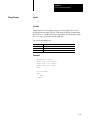
Operators
An operator combines or compares values of operands: constants and
variables. Operators (except negation) take two operands and perform
some operation to produce a result. This result is generally the same type
as the operands. The table on the following page lists the operators
available and the types they accept and produce.
Operators have precedence which means they are evaluated in a specific
order (for example, multiplication is performed before addition). You can
use parentheses to override natural precedence. The compiler, however,
may remove extraneous parentheses. The legal operators are listed below,
in order from highest to lowest.
Table 2.D
Legal Operators
Highest Precedence
NOT
–(negate)
^
**
*
/
+
–
>
<
<>
=
>=
<=
AND
Lowest precedence
OR
XOR
Operators of equal precedence are shown on the same line, and are
evaluated left to right in expressions. The only exception to this rule is
exponentiation, which is evaluated right to left. Raising a negative number
to a power is not legal in BASIC.
2-10
Chapter 2
Getting Started
In the examples below, BASIC expressions on the left are evaluated as
indicated on the right. You may enter either form, but the compiler always
generates the simpler form on the left.
BASIC representation:
Equivalent form
a:= b+c**2/d
a:= b+((c**2)/d)
a:= b>c AND d>e OR c=e
a:= ((b>c) AND (d>e)) OR (c=e)
a:= (b+c+d)/e
a:= ((b+c)+d)/e
a:= b**c**d/e
a:= (b**(c**d))/e
a:= –(b)**2
a:= (–b)**2
a:=b=c
a:= (b=c) (returns BOOLEAN value)
Operator:
Function:
Operand type:
Result type:
–
Negation
NUMERIC
NUMERIC
^ or **
Exponentiation
NUMERIC (positive)
NUMERIC
*
Multiplication
NUMERIC
NUMERIC
/
Division
NUMERIC
NUMERIC
+
Addition
NUMERIC
NUMERIC
–
Subtraction
NUMERIC
NUMERIC
NOT
Logical Negation
BOOLEAN
BOOLEAN
AND
Logical AND
BOOLEAN
BOOLEAN
OR
Logical OR
BOOLEAN
BOOLEAN
XOR
Logical EXCLUSIVE OR
BOOLEAN
BOOLEAN
+
Concatenation
STRING
STRING
=
Equal to
ANY
BOOLEAN
<> or ><
Not equal to
ANY
BOOLEAN
<
Less than
NUMERIC, STRING 1
BOOLEAN
<= or =<
Less than or Equal
NUMERIC, STRING 2
BOOLEAN
>
Greater than
NUMERIC, STRING 3
BOOLEAN
>= or =>
Greater than or Equal
NUMERIC, STRING 4
BOOLEAN
When comparing strings, the ASCII collating sequence is used, so that 0 < 1 < ... < 9 < A < B<
... < Z < a < b< ... < z
Important: NUMERIC refers to either BYTE, INTEGER, or REAL types.
2-11
Chapter 2
Getting Started
Conditional Control: The
IF..THEN Structure
The IF..THEN..ELSE structure is frequently used in programs. The syntax
is as follows:
IF <boolean> THEN
<statement>
ELSE
<statement>
ENDIF
This executes certain statements only if specified conditions exist. The
following example demonstrates the IF..THEN..ELSE structure:
PROCEDURE MESSAGE
PRINT “Type your name.”
INPUT name$
PRINT “Would you like the message of the day, “;name$;”? (y/n)”
INPUT answer$
IF answer$ = “y” THEN
PRINT “Space is the future”
ELSE
PRINT “Suit yourself.”
ENDIF
PRINT “Bye, “; name$; ”. It’s been nice talking to you.”
END
This procedure prints one of two messages depending on your input. The
condition could also depend on a computed value. Also, there could be
many statements or procedures separating the THEN and ELSE segments
of the conditional. This example just shows one of the ways you can use
this structure.
You can also use the IF..THEN statement as a single statement:
IF <boolean> THEN <line#>
This sends the control of the procedure to the specified line number if the
control condition is met. You should rarely use the IF..THEN statement in
this way.
Important: Multiple ELSE statements are not considered errors by the
compiler (that is, they do not generate error signals). However, they do
produce irregular and non-reliable results.
2-12
Chapter 2
Getting Started
Looping Statements
When you write your programs, you may find that you want to repeat a
section of code several times. You can do this using a looping statement.
Loops cause repeated or conditional execution of the statements located
between the starting point and the ending point of the loop. Generally,
loops have one entry at the top and only one exit at the bottom. In this
sense, it becomes one statement, regardless of how many individual
statements it contains.
You can nest loops. This allows the internal statements to be executed even
more times. You should know at least what will happen on the first,
second, next to the last, and last passes through the looping structure. It is
usually during these passes when a procedure produces errors which can
halt execution.
BASIC supports four ways of adding loops into your program:
Type of loop:
Description:
FOR..NEXT
Executes code an exact number of times.
WHILE..DO
Tests for a control variable before executing any code, and performs
only as long as the control statement remains true.
REPEAT..UNTIL
Executes the code at least once regardless of the initial conditions,
and repeats the code as long as a control statement remains valid.
LOOP..ENDLOOP
Tests one or more control variables anywhere within the loop (and
perhaps more than once).
Each loop structure is discussed in greater detail. When you write your
programs, you should use the most appropriate loop for what you want to
accomplish; each loop structure has its own advantages.
As a general comment about loops, the initialization placement is very
important. You can easily create an endless loop (a loop that does not end)
by forgetting to initialize variables or by placing the initialization in the
wrong place. This is especially true when changing from one type of loop
structure to another. You should make sure that you know what happens at
the beginning and end of each loop sequence. This helps reduce the chance
of creating an endless loop.
The FOR..NEXT Loop
The FOR..NEXT loop executes a set of statements a specific number of
times. A FOR..NEXT loop begins with the FOR statement. The FOR
statement initializes the loop, and the NEXT statement ends the loop. The
following is an example of a FOR..NEXT loop:
FOR x=1 TO 3
PRINT “Hi There!”
NEXT x
2-13
Chapter 2
Getting Started
This loop prints the string Hi There! three times. The first time BASIC
encounters the FOR statement, x equals 1 (FOR x=1). BASIC executes the
statement(s) within the loop, which in this example is a PRINT statement.
When it reaches the NEXT statement, it increments x and goes back to the
FOR statement. x now equals 2, so BASIC again executes the PRINT
statement and goes to the NEXT statement. Once again, x is incremented.
x now equals 3. BASIC executes the PRINT statement and goes to the
NEXT statement. This time when the NEXT statement increments x, x is
greater than three. Therefore, BASIC does not execute the PRINT
statement. Instead, it jumps to the statement that follows NEXT.
Using STEP Within a FOR..NEXT Loop
By default, the NEXT statement increments the variable by one each time.
If you want to increment the variable by a value other than one, you need
to include a STEP declaration in the FOR statement. For example:
FOR x=1 to 10 STEP 2
PRINT “Hi There!”
NEXT x
The string Hi There! is printed five times because each time BASIC comes
to the NEXT statement, x is incremented by two. Therefore, after the first
pass through the loop, x equals three instead of two.
The value to STEP may be a positive or negative number, and it may be
either an integer or a real. If it is a real data type (for example, STEP .5)
the control variable must also be a real data type. The following is an
example of a real data type for the STEP value:
DIM x:REAL
FOR x=1 TO 5 STEP .5
PRINT x
NEXT x
END
This example prints the value of x for each pass through the loop.
2-14
Chapter 2
Getting Started
The WHILE..DO Loop
The WHILE..DO loop tests for a control variable before executing any
code. It continues to loop as long as the control statement located in the
WHILE statement remains true. If the control statement in the WHILE
statement is false the first time it is encountered, the loop is not executed.
The WHILE..DO loop has the following syntax:
WHILE <boolean> DO
.
.
ENDWHILE
<boolean> may be an expression (such as x<5) or merely a BOOLEAN
variable (such as WHILE red DO).
The following is an example of a WHILE..DO loop:
x:=1
WHILE x<5 DO
PRINT x
x:=x+1
ENDWHILE
The first line is outside of the WHILE..DO loop, but it is important for this
loop because it initializes the value of x. The next line begins the loop. It
tells BASIC to test the value of x. If x is less than five, then the statements
inside the loop are executed. If the value of x is five or greater, the
statements inside the loop are not executed. Therefore, the output from this
loop looks like this:
1.
2.
3.
4.
Important: You must change the value of the conditional within the loop.
If you do not, the loop never exits. For example, the following is an
endless loop because the internal commands do not affect the
conditional statement:
a:= 5
WHILE a < 10 DO
PRINT “This is an endless loop”
ENDWHILE
2-15
Chapter 2
Getting Started
The REPEAT..UNTIL Loop
Another loop statement is REPEAT..UNTIL. It is similar to the
WHILE..DO statement. The syntax is as follows:
REPEAT
.
.
UNTIL <boolean>
The major difference is that in a REPEAT..UNTIL statement, the
conditional statement is tested at the bottom of the loop. This means that
the statements within the loop are executed at least once, even if the
conditional statement is false the first time.
The following is an example of a loop using REPEAT..UNTIL:
x := 1
REPEAT
PRINT x
x := x+1
UNTIL x>10
Notice again that x is initialized outside of the loop. If it were initialized
inside of the loop, the loop would never end. The next statement, REPEAT,
begins the loop. The statements within the loop are always executed during
the first pass. The UNTIL statement tests the conditional value. If the
statement is false, the loop executes again. If the statement is true, the loop
is not executed again.
Because the variable is tested at the bottom of the loop, it usually has an
opposite test from one you would find in a WHILE loop. You can easily
introduce errors into your program when you change from a WHILE..DO
loop to a REPEAT..UNTIL loop by forgetting to change the
conditional statement.
2-16
Chapter 2
Getting Started
The LOOP..ENDLOOP Loop
The final type of loop structure available in BASIC is the
LOOP..ENDLOOP statement. It has no built-in control statement to test for
exit, so it uses an internal structure, the EXITIF..THEN statement. The
syntax for these two structures are as follows:
LOOP
<statements>
EXITIF <boolean> THEN
<statements>
ENDEXIT
<statements>
ENDLOOP
The LOOP structure would execute endlessly without the EXITIF
construct. You can use the EXITIF structure as many times as needed
within a LOOP. In this way, you may exit a loop for different reasons. The
following is an example of a LOOP..ENDLOOP:
x := 1
LOOP
PRINT “x is a small number”
x := x +1
EXITIF x>3 THEN
PRINT “x is now greater than three”
ENDEXIT
ENDLOOP
The execution of this procedure is similar to the REPEAT..UNTIL. The
loop is executed until x > 3. Then, the statement between the THEN and
the ENDEXIT is executed (PRINT). The loop is then exited.
You can omit the statement to be executed in the EXITIF loop. For
example, you could enter:
EXITIF x>3 THEN
ENDEXIT
This is known as a null statement because nothing occurs.
2-17
Chapter 2
Getting Started
The EXITIF..THEN structure may be used in any of the looping structures
to exit anywhere within the loop. This allows greater freedom in building
your procedures.
Editing Your Procedures
Once you have written a procedure, you can change it by using the editor.
There are a number of commands available in edit mode for this purpose.
They are as follows:
Command:
Description:
<return>
Moves the edit pointer forward one line.
+[<number>]
Moves the edit pointer forward the specified number of lines (default
is 0).
+*
Moves the edit pointer to the end of the procedure.
–[<number>]
Moves the edit pointer back the specified number of lines.
–*
Moves the edit pointer to the beginning of the procedure.
<space> <text>
Inserts a line directly before the current line.
<space> <line#>
<text>
Inserts or replaces a numbered line.
<line#> <return>
Moves edit pointer to specified line.
c[*]<delim><string1>
<delim><string2>
<delim>
Replaces <string1> with <string2> in the current line. If used with an
asterisk (*), the entire procedure is searched and replaced. <delim>
is a delimiter character that is not within either string.
For example:
c.why.why not?.
c?why?why not??
2-18
Legal syntax
Illegal syntax: ? is in the string
d[*] [line#]
Deletes the specified lin. eIf no line is specified, the current line is
delete. dIf a negative number is specified, the specified number of
lines before the current line are delete. The forms d–* or d+* are also
allowed. They delete all lines before or after the current line
respectively. d* deletes the entire procedure.
l[*] [<number>]
Lists the specified number of lines from the current edit pointer. If the
number is negative, the specified number of lines before the current
line is displayed. l* lists the entire procedure.
q
Quits the editor, and returns to system mode.
r[*] [<number>],
[<increment>]
Renumbers the numbered lines in a procedure. The r command
begins at the current line and renumbers the first numbered line
found with the specified number. After that, it increments the line
number by the specified increment. If an asterisk (*) is used, the
renumbering begins with the start of the procedure. This also
renumbers any references to line numbers (GOTO or IF..THEN
statements). The default values for renumbering are a starting value
of 100 with an increment of 10.
s[*] <del> <string>
<del>
Searches for the indicated string on the current line. If an asterisk (*)
is used, the entire procedure is searched and the pointer is moved to
the first matching string. Delimiters (<del>) follow the same rules as
the c command.
<escape>
Quits the editor.
Chapter 2
Getting Started
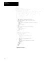
Using the Edit Mode Commands
To use the editor, you must be in edit mode. You can use these commands
to create, display, and edit the procedure mtable. This section goes step by
step. You should enter the commands on your own terminal.
First, enter the command e mtable from the system mode:
B:e mtable
When you have pressed return, the following is displayed:
PROCEDURE mtable
*
Now, enter the procedure. Notice that you can type the procedure all in
lower case characters. When the procedure is displayed, you will see that
all reserved words have been converted to upper case letters. Remember to
add a space before each line.
E: dim a,b: integer
*
E: a:=1
*
E: print
*
E: while a<10 do
*
E:b:=1
What?
The last two lines show what happens when you forget to add the <space>
command before a line. Just re-type the line and continue:
E: b:=1
*
E: while b<=10 do
*
E: print a; “ * “; b; “ = “; a*b; tab(mod(b,5)*13)
*
E: if pos>55 then print
*
E: ednif
ednif
^
Error #000:027
*00AE ERR ednif
E:
2-19
Chapter 2
Getting Started
The last six lines of this section show what happens if you make a mistake
while typing in a command line. If this happens, enter an extra carriage
return and re-type the command line. The line containing the error can be
deleted later.
E:
*
E:
*
E:
*
E:
*
E:
*
E:
*
E:
*
E:
*
E:
endif
b:=b+1
endwhile
print
a:=a+1
endwhile
end
Now that the procedure is entered, type q to exit edit mode:
E:q
Ready
To run the procedure, type run mtable:
B:run mtable
Error #000:051
Ready
2-20
Chapter 2
Getting Started
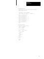
In this example, the procedure will not execute until the line containing the
error is deleted. Therefore, you should re-enter edit mode and use the l*
command to list your program:
B:e mtable
PROCEDURE mtable
*0000
DIM a,b:INTEGER
E:l*
*0000
DIM a,b:INTEGER
0012
a:=1
0020
PRINT
0024
WHILE a<10 DO
003A
b:=1
0048
WHILE b<=10 DO
005E
PRINT a; “ * “; b; “ = “; a*b; TAB(MOD(b,5)*13)
0098
IF POS>55 THEN PRINT
00B0 ERR ednif
00BA
ENDIF
00BE
b:=b+1
00D2
ENDWHILE
00DC
PRINT
00E0
a:=a+1
00F4
ENDWHILE
00FA
END
E:
Notice that the first line of the procedure is displayed with an asterisk (*)
before the line. This points to the location of the edit pointer. Because the
error is on line nine of the procedure, you must move the edit pointer to
line nine. You can use the +<num> command to do this. If you redisplay
the procedure (with the l* command) after executing this command, the
asterisk (*) is now in front of the ninth line.
E:+9
*00B0 ERR ednif
The d command deletes the line:
E:d
*00B0
ENDIF
2-21
Chapter 2
Getting Started
You can now exit edit mode (by typing q) and run the procedure:
E:q
Ready
B:run mtable
1 * 1 = 1
1 * 6 = 6
1 * 2 = 2
1 * 7 = 7
1 * 3 = 3
1 * 8 = 8
1 * 4 = 4
1 * 9 = 9
1 * 5 = 5
1 * 10 = 10
2 * 1 = 2
2 * 6 = 12
2 * 2 = 4
2 * 7 = 14
2 * 3 = 6
2 * 8 = 16
2 * 4 = 8
2 * 9 = 18
2 * 5 = 10
2 * 10 = 20
3 * 1 = 3
3 * 6 = 18
3 * 2 = 6
3 * 7 = 21
3 * 3 = 9
3 * 8 = 24
3 * 4 = 12
3 * 9 = 27
3 * 5 = 15
3 * 10 = 30
4 * 1 = 4
4 * 6 = 24
4 * 2 = 8
4 * 7 = 28
4 * 3 = 12
4 * 8 = 32
4 * 4 = 16
4 * 9 = 36
4 * 5 = 20
4 * 10 = 40
5 * 1 = 5
5 * 6 = 30
5 * 2 = 10
5 * 7 = 35
5 * 3 = 15
5 * 8 = 40
5 * 4 = 20
5 * 9 = 45
5 * 5 = 25
5 * 10 = 50
6 * 1 = 6
6 * 6 = 36
6 * 2 = 12
6 * 7 = 42
6 * 3 = 18
6 * 8 = 48
6 * 4 = 24
6 * 9 = 54
6 * 5 = 30
6 * 10 = 60
7 * 1 = 7
7 * 6 = 42
7 * 2 = 14
7 * 7 = 49
7 * 3 = 21
7 * 8 = 56
7 * 4 = 28
7 * 9 = 63
7 * 5 = 35
7 * 10 = 70
8 * 1 = 8
8 * 6 = 48
8 * 2 = 16
8 * 7 = 56
8 * 3 = 24
8 * 8 = 64
8 * 4 = 32
8 * 9 = 72
8 * 5 = 40
8 * 10 = 80
9 * 1 = 9
9 * 6 = 54
9 * 2 = 18
9 * 7 = 63
9 * 3 = 27
9 * 8 = 72
9 * 4 = 36
9 * 9 = 81
9 * 5 = 45
9 * 10 = 90
Ready
B:
2-22
Chapter 2
Getting Started
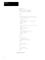
The table looks pretty good now, but it needs a header. To add the header,
re-enter edit mode and display the procedure:
B:e mtable
PROCEDURE mtable
*0000
DIM a,b:INTEGER
E:l*
*0000
DIM a,b:INTEGER
0012
a:=1
0020
PRINT
0024
WHILE a<10 DO
003A
b:=1
0048
WHILE b<=10 DO
005E
PRINT a; “ * “; b; “ = “; a*b; TAB(MOD(b,5)*13)
0098
IF POS>55 THEN PRINT
00B0
ENDIF
00B4
b:=b+1
00C8
ENDWHILE
00CE
PRINT
00D6
a:=a+1
00EA
ENDWHILE
00F0
END
E:
Now, move the edit pointer to the first PRINT statement, and insert a line
to print a header:
E:+2
PRINT
*0020
E: print tab(13); “Multiplication Tables”
*0046
PRINT
E:
Important: Instead of using the +<num> command, you could enter a
carriage return twice.
If you list your program again, the new line is now the third line of
your procedure:
E:l*
0000
0012
0020
*0046
004A
0060
.
.
.
0116
DIM a,b:INTEGER
a:=1
PRINT TAB(13); “Multiplication Tables”
PRINT
WHILE a<10 DO
b:=1
END
2-23
Chapter 2
Getting Started
Now when you run this procedure, your table will have a header.
You should experiment with the edit commands until you feel comfortable
with them. This makes creating and editing your procedures much easier.
Line Numbers and the
GOTO Statement
As mentioned before, the listing Basic displays is not in the exact format as
the input. There is a space between the I-code address and the actual
procedure. This is reserved for line numbers.
Although line numbers are required in many versions of BASIC,
Microware BASIC does not require them. Line numbers must be positive
whole numbers in the range of 1 to 32767. They do not need to be used for
every line. They are generally used with a GOTO or GOSUB statement.
The GOTO statement transfers control unconditionally to the specified
line. For example:
PROCEDURE gotodemo
PRINT “This is a GOTO example”
GOTO 10
PRINT “This line will never be printed”
10 PRINT “It works but it’s dangerous”
END
As you can see, a GOTO statement could cause certain parts of a
procedure’s code to be excluded from execution. There are generally better
ways of obtaining the same results without ever using a GOTO statement.
The use of the GOSUB statement is discussed in detail in Chapter 3.
Important: If at all possible, do not use line numbers or the GOTO
statement. Your procedures will be shorter, faster and easier to edit. There
is less chance of error. If you must use a GOTO statement, use it sparingly
and always document the code with a comment.
2-24
Chapter 2
Getting Started
Putting It All Together
With the various control statements and editing commands presented in
this chapter, you should be able to write some fairly advanced procedures.
For example, the following program was written using just what you have
learned in this chapter:
PROCEDURE multable
DIM less:BOOLEAN
DIM answer$:STRING[1]
DIM a,b,c:INTEGER
PRINT “Type your name”
INPUT name$
PRINT “Hi, “; name$; “! “;
PRINT “Would you like to print a multiplication table?”
PRINT “Type y for yes. Type any other key for no.”
INPUT answer$
IF answer$=”y” THEN
PRINT “What is the number you want to multiply?”
PRINT “(please specify a number between 1 and 100)”
INPUT a
PRINT “What is the range of the multiplication table?”
PRINT “(type 2 numbers between 1 and 50 separated by a space)”
INPUT b,c
WHILE b=c DO
PRINT “Please specify two different numbers for the range.”
INPUT b,c
ENDWHILE
PRINT “Thank you, “; name$
count=1
REPEAT
PRINT b; “ * “; a; “ = “; b*a,
IF POS>55 THEN PRINT
ENDIF
IF b>c THEN b:=b–1
less=FALSE
ELSE
less=TRUE
b:=b+1
ENDIF
UNTIL b=c+1 AND less OR b=c–1 AND NOT(less)
ELSE PRINT “Your loss, “; name$
ENDIF
END
2-25
Chapter
3
Program Construction:
Complex Data Types and Subroutines
Introduction
This chapter discusses the following complex data types and subroutines
that you can use with Microware BASIC:
arrays
TYPE declarations
external files
subroutines
command line parameters
formatted output
Arrays
An array is an ordered sequence of data types. An array may be one, two,
or three dimensional.
A vector is a one-dimensional array.
A table is a two-dimensional array.
A matrix is a three-dimensional array.
The size of an array depends on the number of elements in each dimension
and the size of each element. The array size is declared with a statement.
The syntax for declaring a vector array is as follows:
DIM <array name>(<rows>) : <DATA TYPE> [<num>]
For example, the following line declares the vector array names. Names
has 80 string elements. Each element is 30 characters:
DIM Names(80) : STRING [30]
The syntax for declaring a table array is as follows:
DIM <array name>(<rows>,<cols>) : <DATA TYPE> [<num>]
The following line declares the table array, PHONEBOOK, with the two
dimensions of 80 rows and 5 columns of STRING elements. Each element
is 30 characters.
DIM Phonebook(80,5): STRING [30]
3-1
Chapter 3
Program Construction:
Complex Data Types and Subroutines
The syntax for declaring a matrix array is as follows:
DIM <array name>(<rows>,<cols>,<depth>) : <DATA TYPE> [<num>]
The following line declares the matrix array, Route, with three dimensions
of 5 rows, 5 columns, and 5 depth INTEGER elements. Each element is
25 integers:
DIM Route(5,5,5) : INTEGER [25]
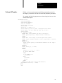
Like variables, you must initialize each array before you use it.
The following procedure initializes Phonebook to null values:
PROCEDURE init
DIM Phonebook(80,5): STRING [30]
DIM x,y : INTEGER
FOR x := 1 TO 80
FOR y := 1 TO 5
Phonebook(x,y) = “”
NEXT y
NEXT x
END
You should initialize numeric array elements to zero in the same manner.
Once an array is initialized, it can be loaded in various ways. The simplest
way is to assign individual element’s values by an assignment statement
which references the specified element:
Phonebook(1,1) := “Larry Crane”
Phonebook(1,2) := “unlisted”
3-2
Chapter 3
Program Construction:
Complex Data Types and Subroutines
Although this is simple, it is extremely time consuming. Instead, you can
use a looping structure and the INPUT statement to load the array:
PROCEDURE Addphone
DIM Phonebook(80,5):STRING[30]
DIM x,y:INTEGER
DIM done:BOOLEAN
DATA “NAME”,“PHONE”,“ADDRESS”,“CITY, STATE”,“ZIP CODE”
done:=FALSE
x:=1
WHILE NOT(done) AND x<=80 DO
FOR y=1 TO 5
READ prompt$
PRINT “ENTER ”; prompt$
INPUT Phonebook(x,y)
NEXT y
INPUT “If finished, type ”“done”“, otherwise <return>.”,flag$
IF flag$=“done” THEN
done:=TRUE
ELSE
x:=x+1
ENDIF
ENDWHILE
END
In this procedure, the DATA and READ statements are used. The READ
statement reads sequentially from the DATA statements output list. When
the list is exhausted, it starts reading from the beginning of the list again.
In this case, Addphone uses the READ statement to change prompts for
each element of the array.
For more information on the DATA and READ statements, refer to the
appropriate reference section.
Notice the INPUT statement following the FOR..NEXT structure:
INPUT “If finished, type ”“done”“, otherwise
<return>.”,flag$
This INPUT statement prints out the character string instead of the regular
question mark (?) prompt. This eliminates an extra PRINT statement.
3-3
Chapter 3
Program Construction:
Complex Data Types and Subroutines
The TYPE Declaration
While the Addphone procedure is adequate for storing names and phone
numbers, an array of varying data types and sizes is more efficient. In the
Phonebook array, each element is thirty characters long, regardless of the
use of the field. A phone number field rarely needs to be greater than
twenty digits. A zip code can be held in nine.
By using the TYPE declaration, BASIC creates user-defined data types. A
user-defined data type may consist of any of combination of the five basic
data types, arrays, and other user-defined data types. For example:
TYPE rec=street:STRING[30];cityst:STRING[30];zip:STRING[9]
TYPE ENTRY=name:STRING[30]; phone:STRING[20]; address:rec
DIM Phonebook(80) : ENTRY
This example is functionally the same array as in Addphone. However, it is
smaller and easier to access. By labeling each field with a descriptive
name, there is no doubt as to what is stored there.
Each field within an element is referred to by the array name and the
number of the element, followed by a period, followed by the field name
(or names each separated by a period):
Phonebook(32).address.zip := 50311
External Files
Once you have defined and accessed variable length records, you need to
save them for future use. The current Addphone program only holds the
memory of the phone number while it is running.
To save the input information, you must open an external file. You can
then place information in this external file.
OS-9 supports two types of files:
Sequential files hold records containing ASCII characters. There can be
any number of characters within a record. There can be any number of
records in a file (within the limits of your disk). Records are separated
by a carriage return.
Random access files contain records that store data in the same manner
as BASIC; in binary. There are no carriage returns to indicate the end of
a record. Records must be of a fixed size. There may be any number of
records in the file (within the limits of your disk).
3-4
Chapter 3
Program Construction:
Complex Data Types and Subroutines
Sequential Files
Sequential files are generally used for text files because of the way data is
accessed. To store data in a sequential file, BASIC supports two
commands: READ and WRITE.
The READ command reads characters from a file until it encounters a
carriage return.
The WRITE command sends each character in the record to the file and
then sends a carriage return to indicate the end of record.
Sequential files must be read one record at a time, starting from where the
file pointer is positioned. Because of the way data is stored in sequential
files, the only way to position the file pointer is to read or write a record.
To access the third record of a sequential file, you must either read the first
two records or rewrite them to place the file pointer at the beginning of the
third record. If you were to rewrite the first record with a new record that is
larger than the original, you will also write over the beginning of the
second record. Obviously, this could cause many problems.
To effectively edit sequential files, you must use a text editor (word
processor, etc.).
Random Access Files
To store data in a random access file, BASIC supports two commands:
The PUT command puts a record in the specified place in your file.
The GET command retrieves the record.
The PUT and the GET statements have the same syntax:
PUT <path no. var> <data struct>
GET <path no. var> <data struct>
You can access data elements in a random access file individually. The
BASIC functions SEEK and SIZE can be used together to locate and place
the file pointer at the beginning of any element. Through proper use of
these functions, you can GET the record you want or PUT any record
where you want it.
3-5
Chapter 3
Program Construction:
Complex Data Types and Subroutines
Creating Files
Before you can access a file, you must first create it. The syntax of the
CREATE statement is as follows:
CREATE
#<int or byte var>, “<path>”: <access mode>
For example, the following command creates the file datafile in the
/h0/USR/ELLEN directory:
CREATE #A “/h0/usr/ellen/datafile”: WRITE
This statement creates the specified file (datafile) and opens a path
number to access it. The CREATE statement assigns a path number to a
variable. The variable must be either an INTEGER or BYTE data type.
The access mode may be any of the following:
Access mode:
Description:
WRITE
Only allows you to send (WRITE/PUT) data to the file.
UPDATE
Allows you to send and receive data (WRITE/PUT and READ/GET).
EXEC
Stores machine language code to be executed. It is rarely used
except by advanced BASIC programmers.
When a file is created, it has a length of zero. It expands automatically as
you send data to it.
Closing Files
When you open a path to a file, you must close it. Notice the line at
the end:
CLOSE #file
The CLOSE statement closes the specified path number. Never close a path
that you did not open, unless absolutely required.
A New Phonebook Example
The following procedure creates a random access file to hold Phonebook
records. It assigns the prompted values to the individual Phonebook data
fields one at a time. It places the entire data structure into the file at
one time.
3-6
Chapter 3
Program Construction:
Complex Data Types and Subroutines
PROCEDURE Phonebook
TYPE rec=street:STRING[30];cityst:STRING[30];zip:STRING[9]
TYPE ENTRY=name:STRING[30]; phone:STRING[20]; address:rec
DIM Phonebook : ENTRY
DIM file : INTEGER
CREATE #file, “phonebook”: UPDATE
PRINT “Enter the information asked for by the prompt”
PRINT “If information not available, hit <return>”
REPEAT
INPUT “name:
”, Phonebook.name
INPUT “phone number:
”, Phonebook.phone
INPUT “street address: ”, Phonebook.address.street
INPUT “city, state:
”, Phonebook.address.cityst
INPUT “zip code:
”, Phonebook.address.zip
PUT #file, Phonebook
PRINT “If finished, type ”“done”“.”
INPUT “Otherwise hit the <return> ”, done$
UNTIL done$ = “done”
CLOSE #file
END
This works if the Phonebook file does not yet exist. However, trying to
CREATE an already existing file causes an error (#218).
To access an already existing file, use the OPEN statement. The OPEN
statement has the same syntax as the CREATE statement:
OPEN #<int or byte var>,“<path>”: access mode
There are five access modes that the OPEN statement uses:
Access mode:
Description:
READ
Reads data from a file.
WRITE
Writes data from a file.
UPDATE
Allows you to read and write to a file.
EXEC
Looks for and stores your file in your execution directory.
DIR
Opens a directory for read only.
You can OPEN a file in more than one mode, if the combination is valid.
For example:
OPEN #file, “example”: READ + EXEC
Important: DIR and either WRITE or UPDATE causes an error. READ +
WRITE is the same as UPDATE.
3-7
Chapter 3
Program Construction:
Complex Data Types and Subroutines
Using A Random Access File
To illustrate the access capabilities of random access files, examine
this procedure:
PROCEDURE Phonebook
TYPE rec=street:STRING[30];cityst:STRING[30];zip:STRING[9]
TYPE ENTRY=name:STRING[30]; phone:STRING[20]; address:rec
DIM Phonebook : ENTRY
DIM file,record : INTEGER
DIM flag : BOOLEAN
flag = TRUE
ON ERROR GOTO 100
CREATE #file, “phonebook”: UPDATE
flag = FALSE
100 IF flag THEN OPEN #file, “phonebook”: UPDATE
ENDIF
ON ERROR
REPEAT
PRINT “Would you like to add or access entries?”
PRINT “Or are you finished for now?”
INPUT “Type ”“add”“, ”“access”” or ”“done”“.”, answer$
IF answer$ = “add” THEN
SEEK #file, FILSIZ (#file)
PRINT “If information not available, hit <return>”
REPEAT
INPUT “name:
”, Phonebook.name
INPUT “phone number:
”, Phonebook.phone
INPUT “street address: ”, Phonebook.address.street
INPUT “city, state:
”, Phonebook.address.cityst
INPUT “zip code:
”, Phonebook.address.zip
PUT #file, Phonebook
PRINT “If finished, type ”“done”“.”
INPUT “Otherwise hit the <return> ”, done$
UNTIL done$ = “done”
ELSE
IF answer$ = “access” THEN
REPEAT
INPUT “What number record would you like?”, record
SEEK #file, SIZE (Phonebook) * (record – 1)
GET #file, Phonebook
PRINT “name:
”, Phonebook.name
PRINT “phone number:
”, Phonebook.phone
PRINT “street address: ”, Phonebook.address.street
PRINT “city, state:
”, Phonebook.address.cityst
PRINT “zip code:
”, Phonebook.address.zip
PRINT “If finished, type ”“done”“.”
INPUT “Otherwise hit the <return> ”, done$
UNTIL done$ = “done”
ENDIF
ENDIF
UNTIL answer$ = “done”
CLOSE #file
3-8
Chapter 3
Program Construction:
Complex Data Types and Subroutines
Important: The BASIC statement ON ERROR GOTO gives control to the
specified line if an error occurs. In this case, it bypasses the problem of
recreating an existing file:
flag = TRUE
ON ERROR GOTO 100
CREATE #file, “phonebook”: UPDATE
flag = FALSE
100 IF flag THEN OPEN #file, “phonebook”: UPDATE
ENDIF
Normally, when an error occurs, the procedure terminates, and BASIC
changes to debug mode. A FALSE value is assigned to flag between the
CREATE and IF..THEN OPEN structure. This assures that only one of the
two access statements (OPEN or CREATE) is executed.
The ON ERROR without the GOTO effectively turns off the previous ON
ERROR statement. This is important, because any other error that might
occur would otherwise be routed to line 100.
Because you can use this procedure to both read and write to the
phonebook file, you must access the file in UPDATE mode.
By prompting for one of three conditions (add, access, or done), you can
channel control to any of these conditions. By placing this control structure
within a REPEAT loop, you may add and access entries in the same
session. By adding REPEAT loops within add and access sections of the
code, you may add or access as many records as desired.
The SEEK statement allows access to the records. In the add loop, the file
pointer is moved to the end of file with the following command:
SEEK #file, FILSIZ (#file)
The SEEK command positions the file pointer directly after the specified
number of bytes. The FILSIZ function returns the size of the file specified
by its path. Consequently, by using both together, the file pointer is
positioned at the end of file.
In the access loop, the SEEK command positions the file pointer at the
beginning of the user-specified record. For simplicity, this procedure uses
numbers to specify records (first record, second record, etc.). The BASIC
function, SIZE, returns the size of the specified data structure. By
multiplying this size by one less than the desired record, the file pointer is
correctly positioned:
SEEK #file, SIZE (Phonebook) * (record – 1)
3-9
Chapter 3
Program Construction:
Complex Data Types and Subroutines
Subroutines
The phonebook procedure is unnecessarily complex. When you repeatedly
use a portion of a procedure, place it in a subroutine. Generally,
subroutines clarify code or avoid repeating the same code throughout a
procedure. In the previous program, you can place the add and access loops
in subroutines to improve clarity.
The GOSUB statement accesses subroutines. The syntax for this structure
is as follows:
GOSUB <line#>
<line#> (subroutine)
RETURN
The GOSUB statement unconditionally passes control to the specified line.
Basic continues to execute sequentially from that point until the RETURN
statement is encountered. Control is then returned to the line immediately
following the GOSUB statement.
Basic supports a related statement that provides better use of subroutines:
ON..GOSUB. The syntax for this statement is as follows:
ON <int expr> GOSUB {<line#>, <line#>}
<line#> (subroutine)
RETURN
<line#> (subroutine)
RETURN
ON..GOSUB evaluates the <int expr> and transfers control to the
corresponding line number in the list following GOSUB. If the integer is
greater than the number of line numbers in the list, no subroutine is
executed. When used with a previous input statement, ON..GOSUB can
run menu-type subroutines.
3-10
Chapter 3
Program Construction:
Complex Data Types and Subroutines
The following is the Phonebook procedure written with subroutines.
PROCEDURE Phonebook
TYPE rec=street:STRING[30];cityst:STRING[30];zip:STRING[9]
TYPE ENTRY=name:STRING[30]; phone:STRING[20]; address:rec
DIM Phonebook:ENTRY; flag:BOOLEAN; file,answer,record:INTEGER
flag := TRUE
ON ERROR GOTO 100
CREATE #file, “phonebook”: UPDATE
flag := FALSE
100 IF flag THEN OPEN #file, “phonebook”: UPDATE
ENDIF
ON ERROR
REPEAT
PRINT “TYPE: ”“1”” for add new entries“
PRINT ”
“”2”“ for access previous entries”
PRINT “
”“3”” for exit procedure“
INPUT answer
ON answer GOSUB 200,300
UNTIL answer = 3
CLOSE #file
END
200 SEEK #file, FILSIZ (#file)
REPEAT
PRINT ”If information not available, hit <return>“
INPUT ”name:
“,Phonebook.name
INPUT ”phone number:
“,Phonebook.phone
INPUT ”street address: “,Phonebook.address.street
INPUT ”city, state:
“,Phonebook.address.cityst
INPUT ”zip code:
“,Phonebook.address.zip
PUT #file, Phonebook
PRINT ”If finished, type “”done“”.“
INPUT ”Otherwise hit the <return> “,done$
UNTIL done$=”done“
RETURN
300 REPEAT
INPUT ”What number record would you like?“,record
SEEK #file,SIZE(Phonebook)*(record –1)
GET #file,Phonebook
PRINT ”name:
“,Phonebook.name
PRINT ”phone number:
“,Phonebook.phone
PRINT ”street address: “,Phonebook.address.street;
PRINT ”city, state:
“,Phonebook.address.cityst
PRINT ”zip code:
“,Phonebook.address.zip
PRINT ”If finished, type “”done“”.“
INPUT ”Otherwise hit the <return> “,done$
UNTIL done$=”done“
RETURN
3-11
Chapter 3
Program Construction:
Complex Data Types and Subroutines
Calling Procedures
Procedures can often be used by other procedures. BASIC allows
procedures to call each other, and a procedure can call itself. The RUN
statement calls an external procedure. BASIC looks first in the workspace,
then the data directory, and finally the execution directory. If it is found
outside the workspace, BASIC loads and runs it. The RUN statement
syntax is as follows:
RUN <proc name> [(<param>) {,<param>}]
The RUN statement can include parameters (a list of values) to pass to the
called procedure. The called procedure must have a PARAM statement
with variables of the same size and data type as the values passed.
Parameters may be any type of data structure.
The syntax for the PARAM statement is as follows:
PARAM <declaration sequence>: <type>
If a parameter is a constant or an expression, it is passed by value. This
means the called procedure can change it, but the changes are not returned
to the calling procedure
If a parameter is a variable, array, or data structure, it is passed by
reference. This means that any changes made to the value of the parameter
are returned to the calling procedure. BYTE data types may only be passed
by reference.
Commas (,) separate items in the declaration sequence. For example:
PARAM a,b: INTEGER
You can declare multiple data types on the same line by using semicolons
(;). For example:
PARAM a,b: INTEGER; c,d: REAL; listing(10): BYTE
3-12
Chapter 3
Program Construction:
Complex Data Types and Subroutines
The following example passes an array of integers by reference. Example
creates the array and passes it to prin. prin prints the array and passes it
back to example. example passes it to reverse which reverses the order of
the array. The reversed array is passed back to example. prin is run once
more to validate the reversal process.
PROCEDURE example
DIM a,intlist(10): INTEGER
FOR a = 1 TO 10
intlist(a) = a
NEXT a
RUN prin(1,10,intlist)
RUN reverse(1,10,intlist)
RUN prin(1,10,intlist)
END
PROCEDURE prin
PARAM a,b,prin(10): INTEGER
DIM c: INTEGER
FOR c = a TO b
PRINT prin(c);“ ”;
NEXT c
PRINT
END
PROCEDURE reverse
PARAM a,b,intlist(10):INTEGER
DIM c, temp(10): INTEGER
FOR c = b TO a STEP –1
temp(b+1–c) = intlist(c)
NEXT c
intlist = temp
END
The output should look like this:
1 2 3 4 5 6 7 8 9 10
10 9 8 7 6 5 4 3 2 1
3-13
Chapter 3
Program Construction:
Complex Data Types and Subroutines
Command Line Parameters
Parameters may also be passed to the main procedure of a BASIC
program. A PARAM statement must also appear in the main procedure.
One major difference between passing parameters between procedures and
passing parameters to the main procedure is that parentheses are not
required to enclose the parameters passed to the main procedure. For
example, the following two statements pass parameters to a main
procedure from the shell.
$ filter –z=myfiles –p=~ –l=11
$ basic makdoc –z=bman 12
A parameter passed to a procedure is determined to be either a string or
numeric argument by the list of parameters given in the PARAM
statement. The parameters may be expressions that result in the correct
data type. For example, the following statement passes the numeric
argument 15 and the string argument thisthat:
$ filter 11+4 ““this” + “that””
Important: If a string parameter is in expression format (as above) or
could be construed as a numeric parameter (12 or 1.5), the parameter must
be within double quotes.
If you run a program from BASIC, you must use parentheses as if the
procedure was being called from another procedure. For example:
run filter(“–z=myfiles”, “–p=~”, “–l=11”)
Optional Parameters
A parameter passing error only occurs if a parameter is accessed that has
not been passed to a procedure. No error occurs, however, if too few or too
many parameters are passed as long as the missing parameters are not
accessed. The variables expecting parameters are not initialized if no
matching parameters are passed. Consequently, you should create some
sort of parameter handling subroutine for procedures receiving fewer
parameters than expected.
By adding a command line parameter to the Phonebook procedure, you can
create a help message for a first time user and an immediate access to
records. The key to this type of strategy is finding whether a parameter has
been passed, and if so, which one.
A second variable (str1) is declared to trap the parameter. It is initialized to
the string oops. If the parameter is not passed, the ON ERROR routine
passes control to the paramcheck routine. If a parameter is passed, str1 is
set to pstr1 and the paramcheck routine is run.
3-14
Chapter 3
Program Construction:
Complex Data Types and Subroutines
In either case, paramcheck examines str1. By isolating the parameter
checking, the program keeps its integrity and allows for easy maintenance.
A question mark option (–?) is added to print a help message. The help
message explains how to use the procedure.
PROCEDURE Phonebook
PARAM pstr1:string
TYPE rec=street:STRING[30];cityst:STRING[30];zip:STRING[9]
TYPE ENTRY=name:STRING[30]; phone:STRING[20]; address:rec
DIM Phonebook:ENTRY; flag:BOOLEAN; file,answer:INTEGER
DIM str1:string
record = 0
flag := TRUE
str1=“oops”
ON ERROR GOTO 5
str1=pstr1
5 RUN paramcheck(str1,answer,record)
ON ERROR
ON ERROR GOTO 100
CREATE #file, “phonebook”: UPDATE
flag := FALSE
100 IF flag THEN OPEN #file, “phonebook”: UPDATE
ENDIF
ON ERROR
REPEAT
IF answer < 1 THEN
PRINT “TYPE: ”“1”“ for add new entries”
PRINT “
”“2”“ for access previous entries”
PRINT “
”“3”“ for exit procedure”
INPUT answer
ENDIF
ON answer GOSUB 200,300
UNTIL answer = 3
CLOSE #file
END
200 SEEK #file, FILSIZ (#file)
REPEAT
PRINT “If information not available, hit <return>“
INPUT “name:
”,Phonebook.name
INPUT “phone number:
”,Phonebook.phone
INPUT “street address: ”,Phonebook.address.street
INPUT “city, state:
”,Phonebook.address.cityst
INPUT “zip code:
”,Phonebook.address.zip
PUT #file,Phonebook
PRINT “If finished, type ”“done”“.”
INPUT “Otherwise hit the <return> ”,done$
UNTIL done$=“done”
answer = 0
RETURN
3-15
Chapter 3
Program Construction:
Complex Data Types and Subroutines
300 REPEAT
IF record = 0 THEN
INPUT “What number record would you like?”,record
ENDIF
SEEK #file,SIZE(Phonebook)*(record –1)
GET #file,Phonebook
PRINT “name:
”,Phonebook.name
PRINT “phone number:
”,Phonebook.phone
PRINT “street address: ”,Phonebook.address.street
PRINT “city, state:
”,Phonebook.address.cityst
PRINT “zip code:
”,Phonebook.address.zip
PRINT “If finished, type ”“done”“.”
INPUT “Otherwise hit the <return> ”,done$
record = 0
UNTIL done$=“done”
answer = 0
RETURN
PROCEDURE Paramcheck
PARAM str1:STRING; answer,record:INTEGER
IF str1 = “–?” THEN
PRINT “Syntax:
phonebook [<opt>]”
PRINT “Function: This is a little black book for phone numbers.”
PRINT “<opt> = –?
prints this message.”
PRINT “
–a
add mode allows you to add phone numbers.”
PRINT “
–r=<rec> specifies the phone number desired.”
PRINT “
<rec> = the record number of the phone/address.”
STOP
ELSE
IF str1 = “–a” THEN
answer = 1
ELSE
IF LEFT$(str1,3)=“–r=” THEN
record = VAL(MID$(str1,4,(LEN(str1)–3)))
answer = 2
ELSE
answer = 0
ENDIF
ENDIF
ENDIF
END
3-16
Chapter 3
Program Construction:
Complex Data Types and Subroutines
Formatted Output: The
PRINT .. USING Statement
BASIC has a powerful output editing capability for generating reports and
other applications where formatted output is required. The output editing
uses the PRINT..USING statement:
PRINT [<path#>] USING <str expr> , <output list>
The string expression is evaluated and used as a format specification. This
contains specific formatting directives for each item in the output list. The
<path#> is optional and can redirect the output to the
corresponding device.
Important: Blanks are not allowed in format strings!
The items in the output list can be constants, variables, or expressions of
any basic type. As each output item is processed, it is matched with a
specification in the format list. The type of each expression result must be
compatible with the corresponding format specification. If there are fewer
format specifications than items in the output list, the format specification
list is repeated again from its beginning as many times as necessary.
A format string has one or more format specifications separated by
commas. There are two kinds of specifications:
those that control output editing of an item from the output list
those that cause an output function by themselves (such as tabbing
and spacing)
There are six basic output editing directives. Each has a corresponding
one-letter identifier:
Identifier:
Description:
R
Real Format
E
Exponential Format
I
Integer Format
H
Hexadecimal Format
S
String Format
B
Boolean Format
The letter is followed by a positive constant number called the field width.
This number indicates the exact number of columns in which to print the
output. It must allow for the data and “overhead” character positions such
as sign characters, decimal points, exponents, etc. The field width must be
between 1 and 255.
3-17
Chapter 3
Program Construction:
Complex Data Types and Subroutines
Some formats have additional mandatory or optional parameters that
control subfields or select editing options. Real and exponential formats
use the fraction field to specify the number of digits to the right of the
decimal point. The fraction field is separated from the field width by a
decimal point. For example, a field width of 10 and a fraction field of 6 is
represented by “10.6.”
All formats can use the justification option. This option specifies whether
the output is to be centered, left, or right justified within the output field.
Fields are commonly right-justified in reports because it arranges them into
columns with decimal points aligned in the same position. The symbols
used in the justification specifications are:
< (left),
> (right),
^ (center).
In the previous prin procedure, the following print statement was used:
PRINT prin(c);“”;
The extra space was added to separate the integers being printed. A similar
result can be obtained by using the PRINT..USING statement:
PRINT USING “I3>”,prin(c);
This formats each integer in a three space print field (I3). The integers are
right justified (>). You should use some caution when formatting. While a
leading sign is not printed (when positive), space for it must be allowed.
I3> only prints two digit integers.
A full explanation of the PRINT..USING statement and each of the format
types can be found in the reference section of this manual.
3-18
Chapter 3
Program Construction:
Complex Data Types and Subroutines
NOTES
3-19
Chapter
4
Program Optimization
General Execution
Performance of BASIC
When you run your procedures, Microware’s BASIC compiler makes
multiple passes through the code. The compiler produces a compressed and
optimized low-level I-code for execution. Compared to other BASIC
languages, program storage is greatly decreased and execution speed
is increased.
High-level language interpreters have a general reputation for slowness.
This is partly because traditional BASIC interpreters compile from text as
they run, and other BASIC interpreters must perform table-searching
during execution.
Microware BASIC, however, is kept at a powerful level so that there is
little performance difference between the execution of I-code and straight
machine-language instructions. Instead, a single, fast, I-code interpretation
often results in many MPU instruction cycles (such as execution of
floating-point arithmetic operations). Also, BASIC Icode instructions that
reference variable storage, statements, labels, etc., contain the actual
memory addresses, so no table searching is ever required. In addition,
BASIC fully exploits the power of the 68000’s instruction set which was
optimized for efficient execution of compiler-produced code.
BASIC I-code is interpreted. Therefore, a variety of entry time tests,
run-time tests, and development aids are available to help in program
development; aids not available on most compilers:
The editor reports errors immediately when they are entered.
The debugger allows debugging using the original program source
statements and names.
The I-code interpreter performs run-time error checking of things such
as array bound errors, subroutine nesting, arithmetic errors, and other
errors that are not detected (and usually crash)
native-compiler-generated code.
4-1
Chapter 4
Program Optimization
Optimum Use of Numeric
Data Types
BASIC includes several different numeric representations (REAL,
INTEGER, and BYTE) and performs automatic type conversions between
them. You can easily write expressions or loops that take at least ten times
longer to execute than is necessary. Some BASIC numeric operators (+, –,
*, /) and control structures (FOR..NEXT) include versions for both REAL
and INTEGER values. The INTEGER versions are much faster and may
have slightly different properties (for example, when you divide INTEGER
values, the remainder is discarded). Converting data types takes time, so
expressions whose operands and operators are of the same type are
more efficient.
INTEGER operations are faster because they generally have corresponding
68000 machine-language instructions. Overall program speed increases
and storage requirements decrease if INTEGERs are used whenever
possible. INTEGER arithmetic operations use the same symbols as REAL,
but BASIC automatically selects the INTEGER operations when working
with an integer-value result. Only if all operands of an expression are of
types BYTE or INTEGER will the result also be INTEGER.
Sometimes you can get similar or identical results in a number of different
ways at various execution speeds. For example, if the variable value is an
integer, value*2 is a fast integer operation. However, if the expression is
value*2., the value 2. is represented as a REAL number, and the
multiplication is a REAL multiplication which also requires that the
variable value must be transformed into a REAL value, and finally the
result of the expression must be transformed back to an INTEGER value if
you assign it to a variable of that type. Therefore, a single decimal point
slows down this operation by about ten times.
Looping Quickly
When Basic identifies a FOR..NEXT loop structure with an INTEGER
loop counter variable, it uses a special integer version of the FOR..NEXT
loop. This is much faster than the REAL-type version and is generally
preferable. Other kinds of loops also run faster if INTEGER type variables
are used for loop counters.
When writing program loops, remember that statements inside the loop
may be executed many times for each single execution outside the loop.
Thus, any value which can be computed before entering a loop increases
program speed.
4-2
Chapter 4
Program Optimization
Optimum Use of Arrays and
Data Structures
BASIC internally uses INTEGER numbers to index arrays and complex
data structures. If the program uses subscripts that are REAL type variables
or expressions, BASIC converts them to INTEGER before they can be
used. This takes additional time, so use INTEGER expressions for
subscripts whenever you can.
Important: The assignment statement (LET) can copy identically sized
data structures. LET is much faster than copying arrays or structures
element-by-element inside a loop.
The PACK Command
The PACK command produces a compressed version of a BASIC
procedure. Depending on the number of comments, line numbers, etc.,
programs execute from 10% to 30% faster after being packed. Minimizing
use of line numbers will even speed up procedures that are unpacked.
Eliminating Constant
Expressions and
Sub-Expressions
Consider the expression:
x := x+SQRT(100)/2
It is exactly the same as the expression:
x := x+5
The sub-expression SQRT(100)/2 consists of constants only, so its result
does not vary regardless of the rest of the program. But every time the
program is run, the computer must evaluate it. This time can be significant,
especially if the statement is within a loop. You should calculate constant
expressions or sub-expressions while writing the program.
Fast Input and Output
Functions
Reading or writing data a line or record at a time is much faster than one
character at a time. Also, the GET and PUT statements are much faster
than READ and WRITE statements when dealing with disk files. This is
because GET and PUT use the exact binary format used internally by
BASIC. READ, WRITE, PRINT, and INPUT must perform binary-to-ASCII or
ASCII-to-binary conversions.
4-3
Chapter 4
Program Optimization
Professional Programming
Techniques
You can make a program faster by using efficient algorithms. You can use
algorithms found in most standard BASIC and PASCAL books with little
or no adaptation.
You should use a well-structured programming style that produces
efficient, reliable, readable, and maintainable software. BASIC generates
optimized code for the 68000 to execute. This code is currently the most
powerful 16-bit processor in existence. A computer can only execute what
it is told to execute. No language implementation can make up for an
inefficient program. An inefficient program is evidence of a lack of
understanding of the problem. The result is likely to be hard to understand
and hard to update if program specifications change. The identification of
efficient algorithms and their clear, structured expression is indicative of
professionalism in software design.
4-4
Section
2
BASIC Reference Guide
This section of the manual describes:
BASIC’s four command modes:
Mode:
Description:
SYSTEM
Used for executing system commands.
EDIT
Used for creating/editing procedures.
EXECUTION
Used for running procedures.
DEBUG
Used for testing procedures for errors.
Certain commands in each mode will change BASIC’s mode. The
following is a graphic representation of which commands accomplish this
and what mode they are carried out in.
BASIC Mode Changes
OS–9
BASIC
SYSTEM MODE
$
<eof>
BYE
DIR
LIST
MEM
RENAME
SAVE
DIGITS
CHD
CHX
EDIT
KILL
LOAD
PACK
RUN
EXECUTION MODE
RUNB
BASIC
AUTORUN
END
<crtl E>
STOP
BYE
PAUSE
ERROR
<crtl C>
EDIT MODE
c
d
l
r
s
+
–
<cr>
<space>
q
escape
DEBUG MODE
$
Q
DEG/RAD
BREAK
LET
PRINT
LIST
STEP
TRON
TROFF
DIR
CONT
STATE
Chapter 16
Batch Processing Overview
Syntax Notation Used in System Command Descriptions
Individual descriptions of the available commands in each mode follow. In
order to precisely describe their formats, the following syntax notation
is used.
Notation:
Description:
[]
Items in brackets are optional.
{}
Items in braces can be optionally repeated.
<procname>
A procedure name
<pathlist>
An OS-9 file name
<number>
A decimal or hex number
how to use the edit mode (the editor) to create or modify BASIC
procedures
how to run a BASIC procedure
symbolic debugging of programs
data types and data structures
expressions, operators and functions
BASIC program statements and structure
files and unified input/output
16-2
Chapter
5
System Mode
System Mode Commands
System mode includes commands to:
save, load, and examine procedures
interact with OS-9
control the workspace environment
The following are the system commands:
$
DIR
LOAD
BYE
E/EDIT
MEM
RUN
CHD/CHX
KILL
PACK
SAVE
DIGITS
LIST
RENAME
The BASIC command interpreter processes system commands. The
command interpreter always identifies itself with the B: prompt. You
automatically enter the command interpreter when you start BASIC and
when you exit any other mode. You can enter commands in either upper or
lower-case letters.
Commands such as DIR, MEM, $, and BYE do not operate on specific
procedures, but they may have optional or required parameters. Commands
such as SAVE, LOAD, PACK, KILL, and LIST can operate on a specific
procedure or on all procedures within the workspace.
If the command is used with a specific procedure name, the command is
applied to only that procedure. This example displays the procedure named
justin:
LIST justin
The asterisk is a special name that indicates all procedures in the
workspace. Therefore, if you enter the following command, all procedures
in the workspace are displayed:
LIST*
If you do not enter a name with the command, the current working
procedure is used. The current working procedure is the procedure
specified for the last command. The DIR command prints an asterisk
before the current working procedure’s name. This allows you to check
which procedure is current.
5-1
Chapter 5
System Mode
If you have not yet given a name in any command, BASIC automatically
uses the name Program. Some commands require a file name and (one or
more) procedure names. They usually require that a greater-than sign (>)
precede the file name so that it is not mistaken for a procedure name. If
you omit the file name, the name of the (first) procedure is used.
Important: In this manual, the phrase file name means an OS-9 pathlist
which describes either a file or device.
Here are some examples:
SAVE tom bill >myfile
SAVE* big_file
SAVE tic tac toe
(same as SAVE tic,tac,toe >tic)
The RUN and EDIT commands use only one procedure name, or the
current working name if a name is omitted. These commands change
BASIC’s mode by exiting the command mode and entering another mode.
Command:
Description:
RUN
Enters execution mode to run a procedure.
EDIT
Enters edit mode to create or change a procedure.
Important: You cannot directly enter debug mode from system mode.
5-2
Chapter 5
System Mode
$
Shell Command
Syntax
$ [<text>]
Function
This command calls the OS-9 shell command interpreter to process an OS9
command or to run another program. Running the shell command does not
disturb BASIC or its workspace.
If the dollar sign ($) is followed by text, the shell is called to process the
text as a single OS-9 command line. After the command is executed,
BASIC is immediately re-entered.
If no text is specified, BASIC is suspended, and the OS-9 shell is called to
process multiple command lines individually entered from the keyboard.
BASIC regains control when an end-of-file character (usually escape) is
entered. The contents of the BASIC workspace are not affected. This is a
convenient way to temporarily leave BASIC to manipulate files or perform
other housekeeping tasks.
This command is the gateway from BASIC to OS-9. It allows access to
any OS-9 command or to other programs. It also permits creation of
concurrent processes and other real-time functions.
Examples
Command:
Description:
B: $copy file1 file2
Calls the OS-9 copy command
B: $r68 sourcefile&
Calls the assembler as a background task
B: $basic fourier(20)&
Starts another concurrent BASIC program
5-3
Chapter 5
System Mode
BYE (or <eof> character)
Exit Basic
Syntax
BYE
Function
BYE exits BASIC and returns to OS-9 or the program that called BASIC.
Any procedures in the workspace are lost if not previously saved. The
end-of-file character (usually the escape key) does the same thing.
CHD/CHX
Change Directories
Syntax
CHD <pathlist>
CHX <pathlist>
Function
changes the current OS-9 user data directory to the specified pathlist
which must be a directory file. BASIC uses the data directory to LOAD or
SAVE procedures.
CHD
CHX changes the current OS-9 user execution directory to the specified
pathlist which must be a directory file. The execution directory is used to
PACK or auto-load packed modules.
Example
CHD /d1/joe/games
5-4
Chapter 5
System Mode
DIGITS
Formats Numerical Output (Real Numbers)
Syntax
DIGITS [<number>]
Function
DIGITS controls
the number of digits that are printed when REAL numbers
are output.
DIGITS also
controls the precision of transcendental calculation. The
minimum precision is 1 digit to the right of the decimal point, and the
maximum precision is 15. If the result is not within this range (1 to 15
precision), the result is brought into range without error. When no
<number> is specified, DIGITS displays the current precision.
Example
PROCEDURE Digitsdemo
DIM x: REAL
DIGITS 2
INPUT x
PRINT x
END
RUN Digitsdemo
? 44.9234692
44.
DIR
Display Directory of Workspace
Syntax
DIR [<pathlist>]
Function
DIR displays the name, size, and variable storage requirement of each
procedure presently in the workspace. The current working procedure has
an asterisk before its name. All packed procedures have a dash before their
name (see PACK). The available free memory within the workspace is also
given. If a pathlist is specified, output is directed to that file or device.
5-5
Chapter 5
System Mode
A question mark next to a data storage size means the workspace does not
have enough free memory to run that procedure.
Important: Do not confuse this command with the OS-9 dir command.
They have completely different functions.
EDIT/E
Enter Edit Mode
Syntax
EDIT [<procname>]
E [<procname>]
Function
EDIT (E) exits system mode and enters edit mode. If the specified
procedure does not exist, a new one is created. See the next chapter for a
complete description of how edit mode works.
Examples
E newprog
EDIT newprog
KILL/KILL*
Delete Procedure from Workspace
Syntax
KILL [<procname> {,<procname>}]
KILL*
Function
KILL deletes the procedure(s) specified by <procname>. KILL* clears the
entire workspace. This process may take some time if there are many
procedures in the workspace.
Examples
KILL formulas
KILL prog1, prog2, prog7
5-6
Chapter 5
System Mode
LIST/LIST*
Display Listing of Procedure
Syntax
LIST [<procname> {,<procname>}] [> <pathlist>]
LIST* [<pathlist>]
Function
LIST prints a formatted listing of one or more procedures. LIST* prints a
formatted listing of all procedures in the workspace. The listing includes
the relative I-code storage addresses in hexadecimal format in the first
column. The second column is reserved for program line numbers (if line
numbers are used).
If a pathlist is given, the listing is output to that file or device. This option
is commonly used to print hard-copy listings of programs.
LIST
prints on the OS-9 standard error path (#2) if no pathlist is given.
Important: If an asterisk (*) is used, the file name (<pathlist>) follows
immediately without a greater-than sign (>) before it.
Examples
LIST* /p
LIST prog2,prog3 >/p
LIST prog5 >temp
5-7
Chapter 5
System Mode
LOAD
Load Procedure into Workspace
Syntax
LOAD <pathlist>
Function
LOAD loads all procedures from the specified file into the workspace. As
procedures are loaded, their names are displayed. If any of the procedures
being loaded have the same name as a procedure already in the workspace,
the existing procedures are erased and replaced with the procedure
being loaded.
If the workspace fills up before the last procedure in the file is loaded, an
error (#32) is given. In this case, not all procedures may have been loaded,
and the one being loaded when the workspace became full may not be
completely loaded. You should KILL the last procedure, use the MEM
command to get more memory or KILL unnecessary procedure(s) to free
up space, and then LOAD the file again.
Example
LOAD quadratics
MEM
Display or Request Workspace Memory
Syntax
MEM [<number>]
Function
MEM used without a number displays the present total workspace size in
(decimal) bytes. If a number is given, BASIC asks OS-9 to expand or
contract the workspace to that size. A hex value can be used if preceded by
a dollar sign. If MEM responds with What?, you either asked for more
memory than is available, tried to give back too much memory (there has
to be enough to store all procedures in the workspace), or gave an
invalid number.
5-8
Chapter 5
System Mode
Example
MEM 18000
PACK/PACK*
Pack Procedure
Syntax
PACK [<procname> {,<procname>}] [> <pathlist>]
PACK* [<pathlist>]
Function
PACK causes an extra compiler pass on the specified procedure(s). This
removes names, line numbers, non-executable statements, etc. The result is
a smaller, faster procedure(s) that cannot be edited or debugged but can be
executed by BASIC or by the BASIC run-time-only program called RunB.
If a pathlist is not specified, the name of the first procedure in the list is
used as the file name. The packed file is stored in your execution directory.
The procedure is written to the file/device specified in OS-9 memory
module format suitable for loading in ROM or RAM outside the
workspace. BASIC automatically loads the packed procedure when you try
to run it later. Here is an example sequence that demonstrates packing a
procedure:
PACK sort
KILL sort
RUN sort
KILL sort
Packs procedure sort and creates a file
Kills procedure inside the workspace
Run (sort is loaded outside of the workspace)
Done; delete sort from outside memory
The last step does not have to be done immediately if you will be using the
procedure again later, but you should kill it when you are done so its
memory can be used for other purposes.
Important: The packed file cannot be loaded into the workspace later on.
Always perform a regular SAVE before packing a procedure.
Example
PACK proc1,proc2 >packed.programs
5-9
Chapter 5
System Mode
RENAME
Rename a Procedure
Syntax
RENAME <procname>,<new procname>
Function
RENAME changes
the name of a procedure. It can be used to allow two
copies of the same procedure in the workspace under different names.
Example
RENAME thisproc thatproc
RUN
Execute a Procedure
Syntax
RUN [<procname> [ ( <expr> , {<expr>} ) ]]
Function
executes the specified procedure. BASIC leaves system mode and
enters execution mode.
RUN
You can use a parameter list to pass expected parameters to the procedure.
This is generally used in the same way that a RUN statement inside a
procedure calls another procedure. The only restriction is that all
parameters must be constants or expressions without variables. See the
PARAM statement description.
The procedure called can be normal or packed. If the procedure is not
found inside BASIC’s workspace, BASIC calls OS-9 to attempt to LINK
to an external (outside the workspace) module. If this fails, BASIC
attempts to LOAD the procedure from a file of the same name.
Examples
RUN
RUN
RUN
RUN
5-10
getdata
invert(“the string to be inverted”)
power(12,354.06)
power($32, sin(pi/2))
Chapter 5
System Mode
SAVE/SAVE*
Write Procedure to an Output File
Syntax
SAVE [<procname> { <procname>} [> <pathlist>]]
SAVE* [<pathlist>]
Function
SAVE writes the procedure(s) (or all procedures with SAVE*) to an output
file or device in source format. SAVE is similar to the LIST command
except the output is not formatted and I-code addresses are not included. If
a pathlist is not specified, it defaults to the name of the first
procedure listed.
If a file of the same name already exists, SAVE prompts with
the following:
rewrite?
You may answer Y for yes which causes the existing file to be rewritten
with the new procedure(s); or N to cancel the SAVE command.
Important: If an asterisk (*) is used, the file name (<pathlist>) follows
immediately without a greater-than sign (>) before it.
Examples
SAVE proc2 proc3 proc4 >monday.work
SAVE* newprogram
SAVE
SAVE >testprogram
5-11
Chapter
6
Edit Mode
Edit Mode Commands
You use the edit mode (the editor) to create or modify BASIC procedures.
To enter edit mode from system mode, use the EDIT (or E) command.
When you enter edit mode, the prompt E: is displayed. If you have used a
text editor before, you will find the BASIC editor similar to many others
except for these two differences:
The editor is both string and line number oriented. Using line numbers
is optional, and you can correct text without re-typing the entire line.
The editor is interfaced to the BASIC compiler and decompiler. This
lets BASIC perform continuous syntax error checking and allows
programs to be stored in memory in a more compact, compiled form.
The editor includes the following commands. Each command is described
in detail later in this chapter.
Command:
Description:
<cr>
Moves the edit pointer forward one line.
+[<number>]
Moves the edit pointer forward.
–[<number>]
Moves the edit pointer backward.
<space> <text>
Inserts an unnumbered line.
<space> <line#> <text>
Inserts or replaces a numbered line.
<line#> <cr>
Finds a numbered line.
c
Changes a string.
d
Deletes a line.
l
Lists line(s).
q
Quits editing.
r
Renumbers line.
s
Searches for string.
<esc>
Quits editing.
6-1
Chapter 6
Edit Mode
How the Editor Works
BASIC programs are always stored in memory in a compiled form called
I-code (short for Intermediate Code). I-code is a complex binary coding
system for programs that lies between your original source program and
the computer’s native machine language. I-code is relatively compact, can
be executed rapidly, and most importantly, can be reconstructed almost
back to the original source program. The editor is closely connected to the
compiler and decompiler systems within BASIC that translate source code
to I-Code and vice-versa.
When you enter or change a program line and press the return key, the
compiler instantly translates this text to the internal I-code form. When
BASIC displays program lines, it uses the decompiler to translate the
I-code back to the original source format. These processes are completely
automatic and do not require any special action on your part.
This technique has several advantages:
It allows the text editor to report many (syntax) errors immediately so
you can correct them instantly.
The I-code representation of a program is more compact (by about 30%)
than its original form. This allows you to have larger programs in any
given amount of available memory.
When BASIC lists programs, they may appear slightly different than the
way they were originally typed in, but they are always functionally
identical to the original form. A different appearance can happen if the
original program had extraneous spaces between keywords, unnecessary
parentheses in expressions, etc. BASIC keywords are always automatically
capitalized.
When you finish editing the procedure, use the q (for quit) command to
exit edit mode and return to system mode. When you enter the q command,
the compiler passes over the entire procedure again. At this time, syntax
that extends over multiple lines is checked and errors reported. Examples
of these errors are:
GOTO or GOSUB to a non-existent line
missing variable or array declarations
improperly constructed loops
These errors are reported using an error code and the hexadecimal I-code
address of the error. For example:
01FC ERR #000:043
6-2
Chapter 6
Edit Mode
This message means that error number 43 was detected in the line that
included I-code address 01FC (hexadecimal). The LIST command gives
the I-code addresses so you can locate lines with errors reported during the
compiler’s second pass.
Line-Number Oriented
Editing
The editor can work on programs with or without line numbers. If you use
line numbers, they must be positive whole numbers in the range of
1 to 32767.
If you have used another version of the BASIC language, this is the kind of
editing you probably used. However, well-structured programs seldom
really need line numbers. Do not use line numbers unless they are
necessary. By not using line number, your programs will be shorter, faster,
and easier to read.
The line-number oriented commands are:
Command:
Description:
<space> <line#> <text>
Inserts or replaces a numbered line.
<line#> <cr>
Finds a numbered line.
r
Renumbers a line.
r*
Renumbers all lines.
To enter or replace a numbered line, enter a <space>, followed by the line
number and statement. You can enter numbered lines in any order, but they
are stored in ascending sequence. To move the edit pointer to a numbered
line, type the line number followed by a carriage return. The editor moves
to that line (or the line with the next higher number if the specified number
is not found) and displays it. You can delete the line with the d command.
The r renumber command uniformly resequences all numbered lines and
lines that refer to numbered lines. The syntax for this command is
as follows:
r [ <beg line #>
r*[ <beg line #>
[,<incr> ] ] [CR]
[,<incr> ] ] [CR]
The first format renumbers the program starting at the current line and
moving forward to the end of the procedure. Lines are renumbered using
<beg line#> as the initial line number. <incr> is added to the previous line
number for the next line’s number. The following example gives the first
line number 200, the second 205, etc. If <beg line#> and/or <incr> are not
specified, the values 100 and 10, respectively, are assumed.
r 200,5
The second form of the command renumbers all lines in the procedure.
6-3
Chapter 6
Edit Mode
String-Oriented Editing
Most editor commands are string-oriented, which means that you can enter
or change whole or partial lines without using line numbers.
String-oriented editing is generally fast and convenient.
Because line numbers are not used, the editor maintains an edit pointer to
indicate which line is the present working location within the procedure.
String-oriented commands work relative to this point.
The editor shows you the location of the edit pointer by displaying an
asterisk (*) at the left side of the program line where the edit pointer is
presently located.
Moving the Edit Pointer
Use the addition (+) and subtraction (–) commands to reposition the
edit pointer:
Command:
Description:
– <number>
Moves backward <number> lines.
–*
Moves to the beginning of the procedure.
+
Moves forward one line.
+ <number>
Moves forward <number> lines.
+*
Moves to the end of procedure.
The <number> indicates how many lines to move. Backward means
towards the first line of the procedure. If the number is omitted, one is used
(this is true of most edit commands).
A line consisting of a carriage return only moves the pointer forward one
line, which makes it easy to step through a program one line at a time.
Therefore, the following commands all do the same thing:
[CR]
+ [CR]
+1 [CR]
Inserting Lines
The insert line function consists of a space followed by a BASIC statement
line. The statement is inserted just ahead of the edit pointer position. The
space itself is not inserted.
6-4
Chapter 6
Edit Mode
Deleting Lines
The d command deletes one or more lines:
d [<number>] [CR]
d*
The first form deletes the specified number of lines starting at the edit
pointer’s current position. If the number is negative, that many lines before
the current line are deleted. If a line number is omitted, only the current
line is deleted.
The second form deletes all lines in the procedure. The editor also accepts
two variations of this command:
Command:
Description:
d+*
Deletes all lines to the end of the procedure.
d–*
Deletes all lines to the beginning of the procedure.
Important: Be careful when using the d* command. You may delete
lines unintentionally.
Listing Lines
The l command displays one or more lines:
l [<number>] [CR]
l*
The first form displays the specified number of lines starting at the edit
pointer’s current position. If the number is negative, previous lines
are listed.
The second form displays the entire procedure. Neither form changes the
edit pointer’s position. The line that is the current position of the edit
pointer is displayed with a leading asterisk.
Search: Finding STRINGS
A string is a sequence of one or more characters. This can include letters,
numbers, or punctuation, in any combination. Strings allow you to change
or locate a portion of a statement without having to type the
entire statement.
6-5
Chapter 6
Edit Mode
In the editor, strings must be surrounded by delimiters. Delimiters are two
matching characters located at the beginning and the end of a string. The
editor uses delimiters to locate the beginning and the end of strings. The
characters used for delimiters are not considered part of the string.
Therefore, the character you use for a delimiter must not appear within
the string.
Do not confuse the strings used by the editor with BASIC’s data type
which is also called STRING –. Although they have the same name, they
are quite different.
You can use the s command to locate the next occurrence or all
occurrences of a string. The format for this command is as follows:
s <delim> <match str> [<delim>] [CR]
s*<delim> <match str> [<delim>] [CR]
The first format searches for the <match str> starting with the current line.
If any line at or following the edit pointer includes a sequence of characters
that match the search string, the edit pointer is moved to that line and the
line is displayed. If the string cannot be located, the following message is
displayed and the edit pointer remains at its original position:
CAN’T FIND: “<match str>”
The s* variation searches for all occurrences of the string in the procedure
starting at the present edit pointer and displays all lines in which it is
found. The edit pointer is moved to the last line where the string occurred.
Here are some examples:
Command:
Description:
E:s/counter/
Looks for the string: counter
E:s.1/2.
Looks for the string: 1/2
E:s?three blind mice?
Looks for the string: three blind mice
Change: STRING Substitution
The change string function can eliminate a tremendous amount of typing.
It allows strings within lines to be located, removed, and replaced by
another string. This command is commonly used for fixing error lines
without having to retype the entire line or changing a variable name
throughout a program. The format for the c command is as follows:
c <delim> <match str> <delim> <repl str> [<delim>] [CR]
c*<delim> <match str> <delim> <repl str> [<delim>] [CR]
6-6
Chapter 6
Edit Mode
In the first form, the editor looks for the first occurrence of the match
string starting at the present edit pointer position. If found, the match string
is removed from the line and the replacement string is inserted in its place.
The second form works the same way, except it changes all occurrences of
the match string in the procedure starting at the edit pointer’s
current position.
The c* command stops when it finds or creates a line with an error.
Important: Sometimes you can inadvertently change a line you did not
intend to change because the match string is imbedded in a longer string.
For example, if you attempt to change no to yes and the word normal
occurs before the no you are looking for, normal will change to yesrmal.
Examples
c/xval/yval/
c*,GOSUB 5300,GOSUB 5500
6-7
Chapter
7
Execution Mode
Running Programs
To run a BASIC procedure, enter:
RUN <procname>
If the procedure you want to run was the last procedure edited, listed,
saved, etc., you can execute it without specifying a procedure name (the
asterisk (*) shown in the DIR command identifies this procedure).
If the procedure expects parameters, you can enter them on the same
command line. They must all be constant numbers or strings, as
appropriate, and must be given in the correct order. For example:
RUN add(4,7)
This calls a program (such as the one that follows) and passes it the
specified parameters.
PROCEDURE add
PARAMETER a,b a,b receive the values 4,7
PRINT a+b
END
The ability to pass parameters to a program allows you to specifically
initialize program variables. Sometimes certain procedures are parts of a
larger software system and are designed to be called from other
procedures. You can use this feature to individually test such procedures by
passing them test values as parameters.
When you execute the RUN statement, BASIC enters execution mode. The
procedure runs until one of the following events occur:
an END or STOP statement is executed
you type [Ctrl-E]
a run-time error occurs
you type [Ctrl-C] (keyboard interrupt)
Important: In the first two cases, you return to system mode. In the last
two cases, you enter debug mode.
7-1
Chapter 7
Execution Mode
Execution Mode: Technically
Speaking
The RUN statement is simple and normally you do not need to know what
is happening inside BASIC when you use it. The technical description of
execution mode that follows is given for the benefit of advanced
BASIC programmers.
Execution mode is BASIC’s state when you run any procedure. It involves
executing the Icode of one or more procedures inside or outside the
workspace. Many procedures can be in use because they can call each
other (or themselves) and nest exactly like subroutines.
You can enter execution mode in two ways:
the RUN system command
BASIC’s auto-run feature
The auto-run feature allows BASIC to get the name of a file to load and
run from the same command line used to call BASIC. The file can be
either a SAVED file in the data directory or a PACKED file in the
execution directory. The file may contain several procedures; the one
executed is the one with the same name as the file. Parameters may be
passed following the specified pathname. When using the auto-run feature,
upon finishing execution, control returns to BASIC’s command mode. For
example, the following OS-9 command lines use this feature:
$ BASIC printreport “Past Due Accounts”
$ BASIC evaluate COS(7.8814)/12.075,–22.5,129.055
7-2
Chapter
8
Debug Mode
Overview of Debug Mode
Symbolic debugging is the testing and manipulation of programs using the
actual names and program statements used in the program. This is
accomplished by BASIC’s powerful symbolic debugging commands:
$
BREAK
CONT
DEG/RAD
DIR
LET
LIST
PRINT
Q
STATE
This chapter discusses how the debug mode can let you watch your
program run in slow motion. This allows you to observe each statement as
it is executed. This chapter also includes how to use the debug mode as
a calculator.
Debug mode is entered from execution mode in one of three ways:
when an error occurs during execution of a procedure (that is not
intercepted by an ON ERROR GOTO statement within the program)
when a procedure executes a PAUSE statement
when a keyboard interrupt ([Ctrl-C]) occurs
When any of the above happen, debug mode displays the suspended
procedure name like this:
BREAK: PROCEDURE test5
D:
Important: Debug mode displays a D: prompt when it is waiting for a
command. You can then use any debug mode command to examine or
change variables, turn trace mode on/off, etc. Depending on which
commands are used, execution of the program can be terminated, resumed,
or executed one source line at a time.
8-1
Chapter 8
Debug Mode
$
Shell Command
Syntax
$ <text>
Function
$ calls OS-9’s shell command interpreter to run a program or OS-9
command. This command executes the same as the system mode
$ command.
BREAK
Set Breakpoint
Syntax
BREAK <proc name>
Function
BREAK sets a breakpoint at the specified procedure. This command is used
when procedures call each other and provides a way to re-enter debug
mode when returning to a specific procedure.
To illustrate how BREAK works, suppose three procedures are in your
workspace: Proc1, Proc2, and Proc3. Assume that Proc1 calls Proc2, and
Proc2 calls Proc3. While Proc3 is executing, you type [Ctrl-C] to enter
debug mode. To use the BREAK command, type:
D: BREAK proc1
ok
D:
Important: BREAK responds with ok if the procedure was found on the
current RUN stack. You can use the STATE command to verify that the
three procedures are nested as expected.
You can resume execution of Proc3 by typing cont. After Proc3 terminates,
control passes back to Proc2, which eventually returns to Proc1. As soon as
this happens, the breakpoint you set is encountered, Proc1 is suspended,
and debug mode is re-entered.
8-2
Chapter 8
Debug Mode
There are three characteristics of BREAK you should note:
The breakpoint is removed as soon as it occurs.
You can use one breakpoint for each active procedure.
You cannot put a breakpoint on a procedure unless it has been called but
not yet re-entered. Therefore, BREAK cannot be used on procedures
that have not yet run.
CONT
Continue Execution
Syntax
CONT
Function
CONT continues program execution at the next statement. It may resume
programs suspended by [Ctrl-C], PAUSE statements, BREAK command
breakpoints, or after non-fatal run-time errors.
DEG/RAD
Select Degree or Radian Units for Computation
Syntax
DEG
RAD
Function
The DEG and RAD commands set a state flag. The system uses this state
flag to determine whether degrees or radians (respectively) should be used
as the angle unit for trigonometric functions. These commands only affect
the procedure currently being debugged or run.
8-3
Chapter 8
Debug Mode
DIR
Display Workspace Directory
Syntax
DIR [<path>]
Function
DIR displays the workspace procedure directory in the same way as the
system mode DIR command.
LET
Assignment Statement
Syntax
LET <var> := <expr>
Function
The debug mode LET command is essentially the same as the BASIC LET
program statement. It allows the value of a procedure variable to be set to a
new value using the result of the evaluated expression. The variable names
used in this command must be the same as in the original source program;
otherwise, an error is generated. LET does not work on user-defined data
structures.
LIST
List Current Procedure
Syntax
LIST
Function
displays a formatted source listing of the suspended procedure with
Icode addresses. An asterisk is printed to the left of the statement where the
procedure is suspended. You can only list the current procedure.
LIST
8-4
Chapter 8
Debug Mode
PRINT
Print Present Value of Variables
Syntax
PRINT [#<expr>,] [USING <expr>,] <expr list>
Function
PRINT can be used to examine the present value of variables in the
suspended program. All variable names must be the same as in the original
program. You cannot use new variable names. User-defined data structures
cannot be printed.
Q
Quit Debug Mode
Syntax
Q
Function
terminates execution of all procedures and exits debug mode by returning
to system mode. Any open paths are closed at this point.
Q
STATE
List Calling Order of Procedures
Syntax
STATE
Function
STATE lists the calling (nesting) order of all active procedures. The
highest-level procedure is always shown at the bottom of the calling list,
and the lowest-level procedure is always listed first.
Example
D:state
PROCEDURE
CALLED BY
CALLED BY
CALLED BY
DELTA
BETA
ALPHA
PROGRAM
8-5
Chapter 8
Debug Mode
STEP
Single (or Specified) Line Execution
Syntax
STEP [<number>]
or
[CR]
Function
STEP executes the suspended procedure one or more source statements at
a time.
For example, step 5 executes the equivalent of the next five source
statements. A debug command line which is just a carriage return is
considered the same as step 1. STEP is most commonly used with the trace
mode on. This allows you to see the original source lines as they
are executed.
Important: Because compiled I-code contains actual statement memory
addresses, the top or bottom statements of loop structures are usually
executed just once. For example, in FOR...NEXT loops the FOR statement
is executed once, so the statement that appears to be the top of the loop is
actually the one following the FOR statement.
TRON/TROFF
Turn On/Off Trace Mode
Syntax
TRON
TROFF
Function
These commands turn the suspended procedure’s trace mode on and off. In
trace mode, the compiled code of each equivalent statement line is
reconstructed to source statements and displayed before the statement is
executed. If the statement causes the evaluation of one or more
expressions, an equal sign and the expression result(s) are displayed on the
following line(s).
Trace mode is local to a procedure. If the suspended procedure calls
another, no tracing occurs until control returns to the calling procedure
(unless the called procedure has trace mode on).
8-6
Chapter 8
Debug Mode
Debugging Techniques
If your program does not do what you expect, it is sure to show one of
two symptoms:
premature termination due to an error
incorrect results
The first case automatically sends you into debug mode. In the second
case, you have to force the program into debug mode either by pressing
[Ctrl-C] (assuming you have time to do so), or by using edit mode to put
one or more PAUSE statements in the program. Once you are in debug
mode, you can debug your program.
Usually, after an error stops the program you should use the PRINT
command to look at the present values of crucial program variables. Bad
values are usually quite apparent. Perhaps you forgot to initialize a variable
or forgot to increment a loop counter.
If examining variables is not fruitful, you should place a PAUSE statement
at the beginning of the suspected procedure or at a place within the code
where you think things begin to go wrong. Then, rerun the program. When
the program hits the PAUSE statement, it enters the debug mode.
Next, turn the trace mode on and watch your program run. Type:
D: TRON
Then, press the carriage return key once for every statement you want to
trace. You will see the original source statement, and if expressions are
evaluated by the statement, debug mode prints an equal sign and the result
of the expression.
Notice that some statements such as FOR and PRINT may cause more than
one expression to be evaluated.
Using this technique, you can watch your program run one step at a time
until you see where it goes wrong.
If in the process of tracing, you encounter a loop that works, but executes
200 statements repetitively, you do not have to trace line by line. In this
case, you may turn the trace off and use the STEP command to quickly run
through the loop. Then, turn trace mode back on, and resume single-step
debugging. The command sequence for this is:
D: TROFF
D: STEP 200
D: TRON
8-7
Chapter 8
Debug Mode
Important: Trace mode is local to one procedure only. If the procedure
being tested returns to another procedure you need to use the BREAK
command or put a PAUSE statement in the procedure to enter debug mode.
If you call another procedure from the procedure being debugged, tracing
stops when it is called until it returns. If you also want to trace the called
procedure, it needs its own PAUSE statement.
Debug Mode as a Desk
Calculator
The simple program listed below turns debug mode into a powerful
calculator. Calculator declares 26 working variables, then goes into debug
mode. This allows you to use interactive PRINT and LET statements.
PROCEDURE Calculator
DIM a,b,c,d,e,f,g,h,i,j,k,l,m
DIM n,o,p,q,r,s,t,u,v,w,x,y,z
PAUSE
END
Recall that while in debug mode, you cannot create new variables.
Therefore, DIM pre-defines 26 working variables for you. You can use
more or fewer variables. PAUSE causes you to enter debug mode. The
following is a sample session:
B: run calculator
BREAK: PROCEDURE Calculator
D:let x:=12.5
D:print sin(pi/2)
1.
D:let y:=exp(4+0.5)
D:print x,y
12.5
90.0171313
D:Q
B:
Important: The debug mode PRINT command can use PRINT USING to
produce formatted output (including hexadecimal).
8-8
Chapter
9
Data Types and Data Structures
Data Types
Computer programs process data. The computer’s performance, and even
sometimes whether or not a computer can handle a particular problem,
depends on how the software stores data in memory and operates on it.
BASIC offers many possibilities for organizing and manipulating data.
There are many types of data. You can have numerical data, textual data,
etc., but you can seldom mix data types. Not only do they have different
storage size requirements, but they are logically incompatible. For
example, it would be meaningless to multiply letters and punctuation.
Even within the same general kind of data, there are different ways to
represent data. You can represent numbers in three different ways. Each
way has its own advantages and disadvantages. You should use the way
that fits your needs for each procedure.
To help you select the most appropriate way to store data variables, BASIC
provides five different basic data types. BASIC also lets you create new
customized data types based on combinations of the five basic types.
Data Structures
A data structure refers to storage for more than one data item under a
single name. Data structures can be composed of various data types. Data
structures are often the most practical and convenient way to organize large
amounts of similar data.
The simplest kind of data structure is the array, which is a table of values.
The table has a single name, and the storage space for each individual
value is numbered. Arrays are created by DIM statements.
For example, to create an array having five storage spaces called AGES,
use the statement:
DIM AGES(5):INTEGER
(5) tells BASIC how many spaces to reserve. :INTEGER indicates the
array’s data type. To assign a value of 22 to the third storage space in the
array, use the statement:
LET AGES(3):=22
9-1
Chapter 9
Data Types and Data Structures
The Five Basic Data Types
BASIC includes five basic data types:
Type:
Allowable values:
Memory requirement:
BYTE
Whole Numbers 0 to 255
One byte
INTEGER
Whole Numbers –2,147,483,648 to 2,147,483,647
Four bytes
REAL
Floating Point (+/–) 2.2*10^–308 to 1.8*10^308
Eight bytes
STRING
Letters, digits, punctuation
One byte/character
BOOLEAN
True or False
One byte
REAL numbers appear to be the most versatile data type. They have the
greatest range and are floating-point. Arithmetic operations involving
them, however, are relatively slow (by a factor directly related to the
memory required) when compared to the INTEGER or BYTE types.
Therefore, using INTEGER values for loop counters, indexing arrays, etc.
can significantly speed up your programs. While the BYTE type is not
appreciably faster than INTEGER, it conserves memory space in some
cases and serves as a building block for complex data types in other cases.
If you neglect to specify the type of a variable, BASIC automatically
assumes the REAL data type.
Arrays of any of these data types can be created using one, two, or
three dimensions.
The BYTE Data Type
BYTE variables hold integer values in the range 0 through 255 which are
stored as a single byte. BYTE values are always converted to INTEGER
values and/or REAL values for computation, thus they have no speed
advantage over other numeric types. However, BYTE variables require
only a quarter of the storage used by integers, and an eighth of that used
by reals.
Attempting to store an integer value outside the BYTE range to a BYTE
variable results in the storage of the least-significant 8-bits (the value
modulo 256) without error.
9-2
Chapter 9
Data Types and Data Structures
The INTEGER Data Type
INTEGER variables consist of four bytes of storage. These bytes hold a
numeric value in the range –2,147,483,648 through 2,147,483,647 as
signed 32-bit data. Decimal points are not allowed. INTEGER constants
may also be represented as hexadecimal values in the range $00000000
through $FFFFFFFF to facilitate address calculations. INTEGER values
are printed without a decimal point. INTEGER arithmetic is faster and
requires less storage than REAL values.
Arithmetic which results in values outside the INTEGER range does not
cause run-time errors but instead “wraps around” modulo 4,294,967,296;
(for example, 2,147,483,647 + 1 yields 2,147,483,648). Division of an
integer by another integer yields an integer result, and any remainder is
discarded. Values outside the INTEGER range are converted to REAL
values. Consequently, they return an input error when passed to a
procedure as integers. Additionally, certain functions (LAND, LNOT,
LOR, LXOR) use integer values, but produce results on a non-numeric
bit-by-bit basis.
The REAL Data Type
The REAL data type is the default type for undeclared variables. However,
a variable may be explicitly typed REAL (for example, twopi:REAL) to
improve a program’s internal documentation. REAL-type values are
always printed with a decimal point, and only those constants which
include a decimal point are actually stored as REAL values.
REAL numbers are stored in eight consecutive memory bytes. The
representation is based on the double-precision format of IEEE Draft
Standard 754. Bit 7 of the first byte is the sign of the mantissa. Bits 0-6 of
the first byte and bits 4-7 of the second byte form the exponent. The
exponent is biased by 1024. The remaining 52 bits comprise the mantissa.
The mantissa has an implied leading one bit.
9-3
Chapter 9
Data Types and Data Structures
Internal Representation of
REAL Numbers
BYTE:
+0
s <exponent>
+1
+2
+3
+4
+5
+6
+7
<mantissa>
Mantissa Sign
The exponent covers the range 2.2*10^-308 (2^-1022 through 1.8*10^308
(2^1024)) as powers of 2. Operations which result in values out of the
representation range cause overflow or underflow errors (which may be
handled automatically by the ON ERROR command).
The mantissa covers the range from 1.0 through 1.99999999999999 in
steps of 2^-31. This means that REAL numbers can represent values on the
number line about .0000000005 apart. Operations which cause results
between the representable points are rounded to the nearest
representable number.
Floating point arithmetic is inherently inexact, thus a sequence of
operations can produce a cumulative error. Proper rounding (as
implemented in BASIC) reduces this effect but cannot eliminate it.
Programmers using comparisons on REAL quantities should use caution
with strict comparisons (= or <>), because the exact desired value may not
occur during program execution.
The STRING Data Type
A STRING is a variable length (0 or more) sequence of characters. A
STRING of zero characters is called an empty STRING. A variable may be
defined as a STRING either explicitly (DIM title:STRING) or implicitly
by appending a dollar-sign character to the variable name (title$ := “My
First Program.”).
The default maximum length allocated to each string is 32 characters, but
each string may be dimensioned less (DIM A:STRING [4]) for memory
savings or more (DIM long:STRING [2880]) to allow long strings.
Important: Strings are inherently variable-length entities, and
dimensioning the storage for a string only defines the maximum-length
string which can be stored there.
9-4
Chapter 9
Data Types and Data Structures
When a STRING value is assigned to a STRING variable, the bytes
composing the string are copied into the variable storage byte-by-byte. The
beginning of a string is always character number one, and this is not
affected by the BASE0 or BASE1 statements. Operations which result in
strings too long to fit in the dimensioned storage truncate the string on the
right and no error is generated.
Normally the internal representation of the string is hidden. A string is
stored in a fixed-size storage area and is represented by a sequence of bytes
terminated by the value zero or by the maximum length allocated to the
STRING variable. Any remaining unused storage after the zero byte allows
the stored string to expand and contract during execution.
The example below shows the internal storage of a variable dimensioned
as STRING[6] and assigned a value of SAM. Notice the byte at +3
contains the zero string terminator, and the two following bytes are
not used.
BYTE:
+0
+1
S
+2
A
+3
M
+4
+5
00
If the value ROBERT is assigned to the variable, the zero byte terminator
is not needed because the STRING fills the storage:
BYTE:
+0
+1
R
The BOOLEAN Data Type
+2
O
+3
B
+4
E
+5
R
T
A BOOLEAN data type can have only two values: TRUE or FALSE. They
are stored as single byte values, but they may not be used for numeric
computation. A variable may be typed BOOLEAN (DIM
done_flag:BOOLEAN). BOOLEAN values print out as the character
strings: “TRUE” and “FALSE.”
BOOLEAN values result from comparing two compatible types.
BOOLEAN values are appropriate for logical flags and expressions. For
example, result:=a AND b AND c.
9-5
Chapter 9
Data Types and Data Structures
Do not confuse BOOLEAN operations AND, OR, XOR, and NOT with
the logical functions LAND, LOR, LXOR, and LNOT. Logical functions
use integer values to produce results on a bit-by-bit basis.
Attempting to store a non-BOOLEAN value in a BOOLEAN variable (or
the reverse) causes a binding error or an error on the second compiler pass
when leaving edit mode.
Automatic Type Conversion
Expressions that mix numeric data types (BYTE, INTEGER, or REAL) are
automatically and temporarily converted to the largest type necessary to
retain accuracy. In addition, certain BASIC functions also perform
automatic type conversions as necessary. Therefore, numeric quantities of
mixed types may be used in most cases.
Type-mismatch errors happen when an expression includes types that
cannot legally be mixed. These errors are reported by the second compiler
pass which automatically occurs when you leave edit mode. Type
conversions can take time. Therefore, you should use expressions
containing all values of a single type wherever possible.
Constants
Constants are frequently used in program statements and in expressions to
assign values to variables. BASIC has rules that allow you to specify
constants that correspond to the five basic data types.
Numeric Constants
Numeric constants can be either REAL or INTEGER. If a number constant
includes a decimal point or uses the “E format” exponential form, BASIC
stores the number in REAL format. This is true even if the value could be
represented by an INTEGER or BYTE data type. For example, 8.0.
Therefore, if you want to use a REAL constant, include a decimal point.
This is sometimes done if all other values in an expression are of type
REAL so BASIC does not have to do a time-consuming type conversion
at run-time.
Numbers that do not have a decimal point but are too large to be
represented as integers are also stored in REAL format. The following are
examples of REAL values:
16.0
100000055
9-6
–10.1234567
2.67E+12
–.002
–458.9E–33
Chapter 9
Data Types and Data Structures
Numbers that do not have a decimal point and are in the range of
–2,147,483,648 to +2,147,483,647 are treated as INTEGER numbers.
BASIC also accepts integer constants in hexadecimal in the range 0 to
$FFFFFFFF. Hexadecimal numbers must have a leading dollar sign. The
following are examples of INTEGER values
12
$FEED
Boolean Constants
–2771
$0A
49908
0
$20
The two legal boolean constants are TRUE and FALSE:
DIM flag, state: BOOLEAN
flag := TRUE
state := FALSE
String Constants
String constants consist of a sequence of any characters enclosed in
quotation marks. The binary value of each character byte can be 1 to 255.
Quotation marks can be included in the string by using two quotation
marks in a row to represent one quotation mark.
The null string (“”) is important because it represents a string having no
characters. It is analogous to the numeric zero. The following are STRING
examples:
“BASIC is a microcomputer language”
“AABBCCDD”
“”
(a null string)
“An ”“older woman”“ is wiser”
Variables
Each BASIC variable is local to the procedure where it is defined. Local
means that it is only known to the program statements within that
procedure. You can use the same variable name in several procedures and
the variables will be completely independent. If you want other procedures
to be able to share a variable, you must use the RUN and PARAM
statements to pass the variable when a procedure calls another procedure.
Storage for variables is allocated from the BASIC workspace when the
procedure is called. You cannot force a variable to occupy a particular
absolute address in memory. When the procedure is exited, variable storage
is given back and the values stored in it are lost. Procedures can call
themselves (this is referred to as recursion) which causes another separate
storage space for variables to be allocated.
9-7
Chapter 9
Data Types and Data Structures
ATTENTION: BASIC does not automatically initialize
variables. When a procedure is run, all variables, arrays, and
structures will have random values. Your program must assign
any initial value if needed.
Parameter Variables
Procedures may pass variables to other procedures. When this occurs, the
variables passed to the called procedure are referred to as parameters.
Parameters may be passed in two ways:
Name:
Description:
by reference
This allows values to be returned from the called procedure to calling
procedure variables.
by value
This protects the values in the calling procedure so that the called
procedure cannot change them.
Parameters are usually passed by reference. This is done by enclosing the
names of the variables to be sent to the called procedure in parentheses as
part of the RUN statement. The storage address of each parameter variable
is evaluated and sent to the called procedure, which then associates those
addresses with names in a local PARAM statement.
The called procedure uses this storage as if it had been created locally
(although it may have a new name) and can change the values stored there.
Parameters passed by reference allow called procedures to return values to
their callers.
Parameters may be passed by value by writing the value to be passed as an
expression which is evaluated at the time of the call. Useful
expression-generators that do not alter values are +0 for numbers or +“”
for strings. For example:
RUN
RUN
RUN
RUN
inverse(x)
inverse(x+0)
translate(word$)
translate(word$+“”)
Passes
Passes
Passes
Passes
x by reference.
x by value.
word$ by reference.
word$ by value.
When parameters are passed by value, a temporary variable is created
when the expression is evaluated. The result is placed in temporary
storage. The address of this temporary storage is sent to the called
procedure. Therefore, the value actually given to the called procedure is a
copy of the result, and the called procedure cannot change the variable(s)
in the calling program.
9-8
Chapter 9
Data Types and Data Structures
Important: Expressions containing numeric constants are either
INTEGER or REAL; there is no type BYTE constant. Thus, BYTE-type
variables may be sent to a procedure as parameters, but expressions will be
of types INTEGER or REAL. For example, a RUN statement may evaluate
an INTEGER as a parameter and send it to the called procedure. If the
called procedure is expecting a BYTE-type variable, it uses only the
high-order byte of the (four-byte) INTEGER (which, if the value was
intended to be in BYTE-range, is probably zero.).
Arrays
The DIM statement can create arrays of from one to three dimensions:
A vector is a one-dimensional array.
A table is a two-dimensional array.
A matrix is a three-dimensional array.
The sizes of each dimension are defined when the array is typed (for
example, DIM plot(24,80):BYTE) by including the number of elements in
each dimension.
Therefore, a table dimensioned (24,80) has 24 rows (1-24) of 80 columns
(1 - 80) when accessed in the default (BASE 1) mode. You may elect to
access the elements of an array starting at zero (BASE 0), in which case
there are still 24 rows (now 0-23) and 80 columns (now 0-79). Arrays may
be composed of basic data types, complex data types, or other arrays.
Complex Data Types
The TYPE statement defines a new data type as a vector (a
one-dimensional array) of any basic or previously-defined types.
For example:
TYPE employee_rec = name:STRING; number(2):INTEGER; malesex:BOOLEAN
This structure differs from an array in that the various elements may be of
mixed types, and the elements are accessed by a field name instead of an
array index. For example:
DIM employee_file(250): employee_rec
employee_file(1).name := “Tex”
employee_file(20).number(2) := 115
9-9
Chapter 9
Data Types and Data Structures
The complex structure allows you to store and manipulate related values
that are of many types, to create new types in addition to the five defined
data types, or to create data structures of unusual shape or size. The
position of the desired element in complex-type storage is known and
defined at compile time and need not be calculated at run time. Therefore,
complex structure accesses may be slightly faster than array accesses.
The elements of a complex structure may be copied to another similar
structure using a single assignment operator (:= ). An entire structure may
be written to or read from mass storage as a single entity (for example,
PUT #2, employee_file).
Arrays or complex structures may be elements of subsequent complex
structures or arrays.
9-10
Chapter
10
Expressions, Operators, and Functions
Evaluation of Expressions
Many BASIC statements evaluate expressions. The result of an evaluation
is always a value of some basic type: REAL, INTEGER, STRING, or
BOOLEAN. The expression itself may consist of values and operators. For
example, the expression 5+5 results in an integer with a value of ten.
A value can be a constant value, a variable name, or a function which
returns the result as a value. An operator combines values (typically, those
adjacent to the operator) and also returns a result.
When evaluating an expression, each value is copied to an expression
stack where functions and operators take their input values and return
results. If the expression is used in an assignment statement, the
assignment is made only when the result of the entire expression has been.
This allows the variable which is being modified to be one of the values in
the expression. The same principles apply for numeric, string, and boolean
operators. These principles make assignment statements such as X=X+1
legal in all cases, even though it would not make sense in a
mathematical context.
Any expression evaluates to one of the five basic data types. This does not
mean, however, that all the operators and operands in expressions have to
be of an identical type. Often types are mixed in expressions because the
result of some operator or function has a different type than its operands.
An example is the “less than” operator:
24 < 100
The less-than operator (<) operator compares two numeric operands. The
result of the comparison is of type BOOLEAN; in this case, the
value TRUE.
BASIC allows you to mix the three numeric types because it performs
automatic type conversion of operands. If different types are used in an
expression, the result is the same type as the operand(s) having the largest
representation. As a rule, any numeric type operand may be used in a
expression that is expected to produce a result of type REAL. Expressions
that must produce BYTE or INTEGER results must evaluate to a value that
is small enough to fit the representation. BASIC has a complete set of
functions that can perform compatible type conversion. Type-mismatch
errors are reported by the second compiler pass when leaving edit mode.
10-1
Chapter 10
Expressions, Operators, and Functions
Operators
Operators (excepting negation) perform some operation on two operands.
This produces a result, which is generally the same type as the operands.
The following table lists the operators available and the types they accept
and produce.
Operator:
Function:
Operand type:
Result type:
–
Negation
NUMERIC
NUMERIC
^ or **
Exponentiation
NUMERIC (positive)
NUMERIC
*
Multiplication
NUMERIC
NUMERIC
/
Division
NUMERIC
NUMERIC
+
Addition
NUMERIC
NUMERIC
–
Subtraction
NUMERIC
NUMERIC
NOT
Logical Negation
BOOLEAN
BOOLEAN
AND
Logical AND
BOOLEAN
BOOLEAN
OR
Logical OR
BOOLEAN
BOOLEAN
XOR
Logical EXCLUSIVE OR
BOOLEAN
BOOLEAN
+
Concatenation
STRING
STRING
=
Equal to
ANY
BOOLEAN
<> or ><
Not equal to
ANY
BOOLEAN
<
Less than
NUMERIC, STRING 1
BOOLEAN
<= or =<
Less than or Equal
NUMERIC, STRING 2
BOOLEAN
>
Greater than
NUMERIC, STRING 3
BOOLEAN
>= or =>
Greater than or Equal
NUMERIC, STRING 4
BOOLEAN
When comparing strings, the ASCII collating sequence is used, so that 0 < 1 < ... < 9 < A < B<
... < Z < a < b< ... < z
Important: NUMERIC refers to either BYTE, INTEGER, or REAL types.
10-2
Chapter 10
Expressions, Operators, and Functions
Operator Precedence
Operators have precedence. This means they are evaluated in a specific
order. Parentheses can override natural precedence. However, the compiler
may remove extraneous parentheses. The legal operators are listed here, in
precedence order from highest to lowest:
Precedence:
Operator:
Highest Precedence
NOT
–(negate)
^
**
*
/
+
–
>
<
<>
=
>=
<=
AND
Lowest Precedence
OR
XOR
Operators of equal precedence are shown on the same line, and are
evaluated left to right in expressions. The only exception to this rule is
exponentiation, which is evaluated right to left. Raising a negative number
to a power is not legal in BASIC.
In the following examples, BASIC expressions on the left are evaluated as
indicated on the right. Either form may be entered, but the decompiler
always generates the form on the left:
BASIC representation:
Equivalent form:
a:= b+c**2/d
a:= b+((c**2)/d)
a:= b>c AND d>e OR c=e
a:= ((b>c) AND (d>e)) OR (c=e)
a:= (b+c+d)/e
a:= ((b+c)+d)/e
a:= b**c**d/e
a:= (b**(c**d))/e
a:= –(b)**2
a:= (–b)**2
a:=b=c
a:= (b=c) (returns BOOLEAN value)
10-3
Chapter 10
Expressions, Operators, and Functions
Functions
Functions accept one or more arguments enclosed in parentheses, perform
some operation, and return a value. They may be used as operands in
expressions. Functions expect that the arguments passed to them are
expressions, constants, or variables of a certain type and return a result of a
certain type. Giving a function an argument of an incompatible type results
in an error.
In the descriptions of functions that follow, the following notation
describes the type required for the parameter expressions:
Name:
Description:
<num>
Specifies any numeric-result expression.
<str>
Specifies any string-result expression.
<int>
Specifies any integer-result expression.
The functions below return REAL results. Accuracy of transcendental
functions is 8+ decimal digits. Angles can be either degrees or radians (see
DEG/RAD statement descriptions).
Important: Transcendental functions take a long time to return a value if
passed an extremely large value (for example, SIN(100000000)).
10-4
Name:
Description:
SIN(<num>)
Trigonometric sine of <num>. Result: –1 <= SIN(<num>) <= 1
COS(<num>)
Trigonometric cosine of <num>. Result: –1 <= COS(<num>) <= 1
TAN(<num>)
Trigonometric tangent of <num>.
ASN(<num>)
Trigonometric arcsine of <num>. Result: –PI/2 <= ASN(<num>) <= PI/2
ACS(<num>)
Trigonometric arcosine of <num>. Result: 0 <= ACS(<num>) <= PI
ATN(<num>)
Trigonometric arctangent of <num>. Result: –PI/2 <= ATN(<num>) <= PI/2
LOG(<num>)
Natural logarithm (base e) of <num>, which must be positive.
LOG10(<num>)
Logarithm (base 10) of <num>, which must be positive.
SQR(<num>)
Square root of <num>, which must be positive.
SQRT(<num>)
Square root of <num>; same as SQR.
EXP(<num>)
e (2.71828183) raised to the power <num>, which must be a
positive number.
FLOAT(<num>)
<num> converted to type REAL (from BYTE or INTEGER).
INT(<num>)
Truncates all digits to the right of the decimal point of a REAL <num>.
Examples: INT(0.21) = 0. INT(–2.5) = –2.
PI
The constant 3.141592653589793.
RND(<num>)
If <num>=0, returns random x, 0 <= x < 1.
If <num>>0, returns random x, 0 <= x < <num>.
If <num><0, use ABS(<num>) as new random number seed.
Chapter 10
Expressions, Operators, and Functions
The following functions return results of type INTEGER or BYTE:
Name:
Description:
FIX(<num>)
Rounds REAL <num> and converts to type INTEGER.
MOD(<num1>,<num2>)
Modulus (remainder) function. MOD returns the remainder of <num1>
divided by <num2>. If <num1> is negative, the result is negative.
Examples: MOD(9,5) = 4 ; MOD(–11,3) = –2
ADDR(<name>)
Absolute memory address of variable, array, or structure named <name>.
SIZE(<name>)
Storage size in bytes of variable, array, or structure named <name>.
ERR
Error code of most recent error, automatically resets to zero when
referenced.
PEEK(<int>)
Value of byte at memory address <int>.
WARNING: The specified memory address must be within the limits of
accessible memory space. PEEK(–1) gives a bus error on most systems.
This causes BASIC to abort.
POS
Current character position of PRINT buffer.
ASC(<str>)
Numeric value of first character of <str>.
LEN(<str>)
Length of string <str>.
SUBSTR(<str1>,<str2>)
Substring search: returns starting position of first occurrence of <str1> in
<str2>, or 0 if not found.
INKEY(#<num>)
Returns the number of characters in data buffer.
FILSIZ(#<num>)
Returns size of a file.
The following functions can return any numeric type, depending on the
type of the input parameter:
Name:
Description:
ABS(<num>)
Absolute value of <num>.
SGN(<num>)
Signum of <num>: –1 if <num> < 0; 0 if <num> = 0; or 1 if <num> > 0.
SQ(<num>)
Square <num>.
VAL(<str>)
Convert type STRING to type NUMERIC.
10-5
Chapter 10
Expressions, Operators, and Functions
The following functions perform bit-by-bit logical operations on integer or
byte data types and return integer results. Do not confuse them with the
BOOLEAN-type operators.
Name:
Description:
LAND(<num>,<num>)
Logical AND
LOR(<num>,<num>)
Logical OR
LXOR(<num>,<num>)
Logical EXCLUSIVE OR
LNOT(<num>)
Logical NOT
These functions return a result of type STRING:
Name:
Description:
CHR$(<int>)
ASCII character equivalent of <int>. <int> must be within range
of 0-127.
DATE$
Date and time, format: yy/mm/dd hh:mm:ss.
LEFT$(<str>,<int>)
Leftmost <int> characters of <str>.
RIGHT$(<str>,<int>)
Rightmost <int> characters of <str>.
MID$(<str>,<int1>,<int2>)
Middle <int2> characters of <str> starting at character position
<int1>.
STR$(<num>)
Converts numeric type <num> to displayable characters of type
STRING representing the number converted.
TRIM$(<str>)
<str> with trailing spaces removed.
The following functions return BOOLEAN values:
10-6
Name:
Description:
TRUE
Always returns TRUE.
FALSE
Always returns FALSE.
EOF(#<num>)
End-of-file test on disk file path <num>, returns TRUE if
end-of-file condition exists.
Chapter
11
Program Statements and Structure
Program Structure
A BASIC program can be written as a single procedure, or it may be
divided into a number of smaller procedures, each of which performs a
specific function.
Single procedure programs may be useful when the program is relatively
small. However, large complex programs are generally much easier to
develop, test, and maintain when the program is divided into several
procedures. To do this, you should create a main routine which calls other
BASIC procedures to perform specific functions as subroutines. These
BASIC procedures may in turn call other BASIC procedures in the same
manner. These techniques reflect sound structured programming practice.
A procedure consists of any number of program statement lines. Each line
can have an optional line number. More than one program statement can be
placed on the same line if separated by backslash (\) characters. For
example, the following statements are equivalent:
GOSUB 550 \ PRINT X,Y \ RETURN
GOSUB 550
PRINT X,Y
RETURN
While these statements are functionally equivalent, the second is generally
considered preferable. The first method runs no faster and tends to hide the
structure of the program.
The number of characters on a line is dependent on the content of the line.
In general, lines should be limited to 128 characters or less, to avoid the
generation of errors when BASIC decompiles the I-code for listing
purposes or at run time.
Loop nesting is limited to 39 levels. Nested procedure and subroutine calls
are only limited by stack space.
Program readability is improved if all variables are declared with DIM
statements at the beginning of the procedure, but this is not mandatory.
11-1
Chapter 11
Program Statements and Structure
Line numbers are optional. They can be any integer number in the range of
1 to 32767. Only use line numbers where absolutely necessary (such as
with GOSUB). They make programs harder to understand, use additional
memory space, and increase compile time considerably. Line numbers are
local to procedures. That is, the same line number can be used in different
procedures without conflict.
You can terminate programs with END or STOP statements. These
statements are optional.
Assignment Statements
Assignment statements are used for computing or initializing of variables.
The two assignment statements available with BASIC are LET and POKE.
LET
Assignment State
Syntax
[LET]
[LET]
[LET]
[LET]
<var> := <expr>
<var> = <expr>
<struct> := <struct>
<struct> = <struct>
Function
evaluates an expression and stores the result in <var>. <var> may be a
simple variable or data structure element. The result of the expression
(<expr>) must be of the same or compatible type as <var>.
LET
BASIC accepts either = or := as an assignment operator. However, the
second form (:=) is preferred because it distinguishes the assignment
operation from a comparison (the test for equality). The := operator is also
used in PASCAL.
You can also use the assignment statement to copy the entire value of an
array or complex data structure to another array or complex data structure.
The data structures do not have to have the same type or shape. The only
restriction is that the size of the destination structure be the same or larger
than the source structure.
You can use this type of assignment to perform unusual type conversions.
For example, a string variable of 80 characters can be copied to a
one-dimensional array of 80 bytes.
11-2
Chapter 11
Program Statements and Structure
Examples
A := 0.1
value := temp/sin(x)
DIM array1(100), array2(100)
array1 := array2
LET AUTHOR$ := FIRST_NAME$ + LAST_NAME$
DIM truth,lie:BOOLEAN
lie := 100 < 1
truth := NOT lie
count = total-adjustment
matrix(2).coefficient(n+2) := matrix(1).coefficient(n)
POKE
Store Data at Specific Memory Address
Syntax
POKE <integer expr> , <byte expr>
Function
POKE allows a program to store data at a specific memory address. The first
expression is used as the absolute address to store the type BYTE result of
the second expression. POKE can alter any memory address, so you must be
careful when using it.
ATTENTION: Using POKE with an invalid address causes
BASIC to abort.
11-3
Chapter 11
Program Statements and Structure
Examples
POKE ADDR(buffer)+5,ASC(“A”)
POKE 1200,14
POKE $1C00,$FF
POKE pointer,PEEK(pointer+1)
(* same as alphabet$ := “ABCDEFGHIJKLMNOPQRSTUVWXYZ” *)
FOR i=0 to 25
POKE ADDR(alphabet$)+i,$40+i
NEXT i
POKE ADDR(alphabet$)+26,$00
Control Statements
Control statements affect the sequential execution of program statements.
They are used to construct loops or make decisions that alter program flow.
BASIC provides a selection of loop statements that allow you to create any
kind of loop using sound structured programming style. The control
statements are IF..THEN..ELSE, FOR..NEXT, WHILE..DO,
REPEAT..UNTIL, LOOP..ENDLOOP, GOTO, GOSUB..RETURN, ON
GOTO..RETURN, ON GOSUB..RETURN, and ON ERROR GOTO.
IF..THEN..ELSE
Control Statement
Syntax
IF <bool expr> THEN <statements>
[ ELSE <statements> ]
ENDIF
IF <bool expr> THEN <line #>
Function
The IF structure evaluates an expression to a BOOLEAN value. If the
result is TRUE, the statement(s) immediately following the THEN are
executed. If an ELSE clause exists, statements between the ELSE and
ENDIF are skipped. If the expression is evaluated to FALSE, control is
transferred to the first statement following the ELSE (if present) or to the
statement immediately following the ENDIF.
11-4
Chapter 11
Program Statements and Structure
A special form of the IF statement transfers execution to the statement
having a line number specified if the result of the expression is TRUE. The
line number follows immediately after THEN. This is an implied GOTO
statement. Use this with caution (as all GOTO statements should).
Examples
IF a < b THEN
PRINT “a is less than b”
PRINT “a:”;a;“ b:”;b
ENDIF
IF a < b THEN
PRINT “a is less than b”
ELSE
IF a=b THEN
PRINT “a equals b”
ELSE
PRINT “a is greater than b”
ENDIF
ENDIF
IF payment < balance THEN 400
FOR..NEXT
Control Statement
Syntax
FOR <var> = <expr> TO <expr> [ STEP <expr> ]
NEXT <var>
Function
FOR..NEXT creates a loop that usually executes a specified number of times
while automatically increasing or decreasing a specified counter variable.
The first expression is evaluated and the result is stored in <var>. <var>
must be a simple integer or real variable. The second expression is
evaluated and stored in a temporary variable.
If you use STEP, its expression is evaluated and used as the loop
increment. If the increment is negative, the loop counts down.
11-5
Chapter 11
Program Statements and Structure
The body of the loop (the statements between the FOR and NEXT) is
executed until the NEXT variable (a counter) is larger than the terminating
expression value. For negative STEP values, the loop executes until the
loop counter is less than the termination value. If the initial value of <var>
is beyond the terminating value, the body of the loop is never executed.
You can jump out of FOR..NEXT loops.
ATTENTION: When using REAL control and STEP
expressions, there is a possibility of not completing the number
of loops logically indicated. For example, the following loop
would seem to complete x number of loops. Due to the
rounding nature of REAL numbers, it may only complete
(x – 1) loops:
FOR a = 1/x TO 1 STEP 1/x
.
.
next a
To make sure that the loop is executed the correct number of times, use
INTEGER values for all expressions.
Examples
FOR var = min–1 TO min+max STEP increment-adjustment
PRINT var
NEXT var
FOR x = 1000 TO 1 STEP –1
PRINT x
NEXT x
11-6
Chapter 11
Program Statements and Structure
WHILE..DO
Control Statement
Syntax
WHILE <bool expr> DO
<statements>
ENDWHILE
Function
This loop tests its control expression at the top of the loop. Statements
within the loop are executed as long as <bool expr> is TRUE. The body of
the loop is not executed if the boolean expression evaluates to FALSE
when first executed.
Examples
WHILE a<b DO
PRINT a
a := a+1
ENDWHILE
is equivalent to
100 IF a>=b THEN 500
PRINT a
a := a+1
GOTO 100
500 REM
DIM yes:BOOLEAN
yes=TRUE
WHILE yes DO
PRINT “yes! ”;
yes := POS<50
ENDWHILE
REM reverse the letters in word$
backward$ := “”
INPUT word$
WHILE LEN(word$) > 0 DO
backward$ := backward$ + RIGHT$(word$,1)
word$ := LEFT$(word$,LEN(word$)–1)
ENDWHILE
word$ := backward$
PRINT word$
11-7
Chapter 11
Program Statements and Structure
REPEAT..UNTIL
Control Statement
Syntax
REPEAT
<statements>
UNTIL <bool expr>
Function
This loop tests its control expression at the bottom of the loop. The
statement(s) within the loop are executed until the result of <bool expr> is
TRUE. The body of the loop is always executed at least one time.
Examples
x = 0
REPEAT
PRINT x
x=x+1
UNTIL x>10
is the same as
x=0
100 PRINT x
x=x+1
IF X <= 10 THEN 100
(* compute factorial: n! *)
temp := 1.
INPUT “Factorial of what number? ”,n
REPEAT
temp := temp * n
n := n–1
UNTIL n <= 1.0
PRINT “The factorial is ”; temp
11-8
Chapter 11
Program Statements and Structure
LOOP..ENDLOOP/
EXITIF..ENDEXIT
Control Statement
Syntax
LOOP
<statements>
ENDLOOP
EXITIF <bool expr> THEN <statements>
ENDEXIT
Function
LOOP..ENDLOOP and EXITIF..ENDEXIT are
inherently related. They can be
used to construct loops with tests located anywhere in the body of the loop.
The LOOP and ENDLOOP statements define the body of the loop.
EXITIF clauses can be inserted anywhere inside the loop to leave the loop
if the result of its test is true.
Important: If there is no exit clause, you will create an endless loop.
EXITIF..ENDEXIT allows control to be passed to the next statement outside
the structure containing the EXITIF statement (this includes IF..THEN
statements). EXITIF evaluates an expression to a boolean result. If the
result is TRUE, the statements between the THEN and the ENDEXIT are
executed, and control is transferred outside the binding structure.
Otherwise, the statement following ENDEXIT is executed. This exit clause
is often used to perform some specific function upon termination of the
loop which depends on where the loop terminated.
EXITIF statements
are almost always used when LOOP..ENDLOOP is
used, but they can also be useful in any type of loop or
conditional construct.
11-9
Chapter 11
Program Statements and Structure
Examples
LOOP
is equivalent to
count = count+1
EXITIF count > 100 THEN
done = TRUE
ENDEXIT
PRINT count
ENDLOOP
100 count = count+1
IF count <= 100 THEN
PRINT count
GOTO 100
ELSE
done = TRUE
ENDIF
REM out of loop
INPUT x,y
LOOP
PRINT
EXITIF x < 0 THEN
PRINT “x became zero first”
ENDEXIT
x := x–1
EXITIF y < 0 THEN PRINT “y became zero first”
ENDEXIT
y := y–1
ENDLOOP
GOTO
Control Statement
Syntax
GOTO <line #>
Function
unconditionally transfers execution flow to the line having the
specified number.
GOTO
Important: The line number is a constant, not an expression or a variable.
Example
GOTO 1000
11-10
Chapter 11
Program Statements and Structure
GOSUB..RETURN
Control Statement
Syntax
GOSUB <line #>
.
.
<line#> <statements>
RETURN
Function
GOSUB transfers program execution to a subroutine starting at the specified
line number. The subroutine is executed until a RETURN statement is
encountered which causes execution to resume at the statement following
the calling GOSUB. Subroutines may be nested to any depth.
Example
FOR n := 1 to 10
x := SIN(n)
GOSUB 100
NEXT n
FOR m := 1 TO 10
x := COS(m)
GOSUB 100
NEXT m
STOP
100 x := x/2
PRINT x
RETURN
11-11
Chapter 11
Program Statements and Structure
ON GOTO/ON GOSUB
Control Statement
Syntax
ON <integer expr> GOTO <line #> {,<line #>}
ON <integer expr> GOSUB <line #> {,<line #>}
Function
These statements evaluate an integer expression and use the result to select
a corresponding line number from an ordered list. Control is then
unconditionally transferred to that line number in ON GOTO statements or
as a subroutine in ON GOSUB statements.
These statements are similar to CASE statements in other languages.
Each <line #> in the ordered list is given a value (beginning with
1, 2, 3, ...). <integer expr> must evaluate to a positive INTEGER result
having a value between 1 and N; N being the highest line number in the
list. N is limited by input line length and the number of digits in each line
number. The best case limit for N is 60.
Important: If the expression has a result that does not correspond with the
ordered list, no GOSUB statement is selected and the next sequential
statement is executed.
11-12
Chapter 11
Program Statements and Structure
Example
(* spell out the digits 0 to 7 *)
DIM digit:INTEGER
A$=“one digit only, please”
INPUT “type in a digit”; digit
ON digit+1 GOSUB 10,11,12,13,14,15,16,17
PRINT A$
STOP
10
11
12
13
14
15
16
17
ON ERROR GOTO
(* names of digits *)
A$ := “ZERO”
RETURN
A$ := “ONE”
RETURN
A$ := “TWO”
RETURN
A$ := “THREE”
RETURN
A$ := “FOUR”
RETURN
A$ := “FIVE”
RETURN
A$ := “SIX”
RETURN
A$ := “SEVEN”
RETURN
Control Statement
Syntax
ON ERROR [ GOTO <line #> ]
Function
This statement sets a trap that transfers control to the specified line number
when a non-fatal run-time error occurs. If no ON ERROR GOTO has been
executed in a procedure before an error occurs, the procedure stops and
enters DEBUG mode. You can turn off the error trap by executing ON
ERROR without a GOTO.
This statement is often used with the ERR function which returns the
specific error code, and the ERROR statement which artificially
generates errors.
11-13
Chapter 11
Program Statements and Structure
Important: ERR automatically resets to zero any time it is called.
Example
(* List a file *)
DIM path,errnum: INTEGER; name: STRING[45]
DIM line: STRING[80]
ON ERROR GOTO 10
INPUT “File name? ”; name
OPEN #path,name:READ
LOOP
READ #path, line
PRINT line
ENDLOOP
10 errnum=ERR
IF errnum = 211 THEN
(* end-of-file *)
PRINT “Listing complete.”
CLOSE #path
END
ELSE
(* other errors *)
PRINT “Error number ”; errnum
END
ENDIF
11-14
Chapter 11
Program Statements and Structure
Execution Statements
Execution statements run procedures, stop execution of procedures, create
shells, or affect the current execution of the procedure.
RUN
Run Procedure
Syntax
RUN <proc name> [ ( <param> {,<param>} ) ]
Function
RUN calls a procedure by name. When that procedure ends, control passes
to the statement after the RUN statement. It is most often used to call a
procedure inside the workspace, but it can also be used to call a previously
compiled procedure or a 68000 machine language procedure outside the
workspace. The name can be optionally taken from a string variable.
Parameter Passing
RUN can include a list of parameters enclosed in parentheses to be passed to
the called procedure. The called procedure must have PARAM statements
of the same size and order to match the parameters passed to it by the
calling procedure.
The parameters can be variables, constants, or the names of entire arrays or
data structures. They can be of any type, except variables of type BYTE.
However, BYTE arrays are allowed.
If a parameter is a constant or expression, it is passed by value. A
parameter passed by value is evaluated and placed in a temporary storage
location and the address of the temporary storage is passed to the called
procedure. Parameters passed by value can be changed by the receiving
procedure, but the changes are not reflected in the calling procedure.
If the parameter is the name of a variable, array, or data structure, it is
passed by reference. When passed by reference, the address of that storage
is sent to the called procedure, and the value in that storage may be
changed by the receiving procedure. These changes are reflected in the
calling procedure.
11-15
Chapter 11
Program Statements and Structure
Calling External Procedures
If the procedure named by RUN cannot be found in the workspace, BASIC
checks to see if it was loaded by OS-9 outside the workspace. If it is not
found there, BASIC tries to find a disk file having the same name in the
current execution directory, loads it, and runs it.
In either case, BASIC checks to see if the called procedure is a BASIC
I-code module or a 68000 machine language module and executes it
accordingly. If it is a 68000 machine language module, BASIC executes a
JSR instruction to its entry point and the module is executed as 68000
native code. The machine language routine can return to the original
calling procedure by executing an RTS instruction. The diagram on the
next page shows what the stack frame passed to machine-language
subroutines looks like.
Machine language modules return error status by setting the carry bit of the
MPU condition codes register and by setting the low order word of register
D1 to the appropriate error code. For an example of a machine language
subroutine (SYSCALL), see Appendix A.
After an external procedure has been called but is no longer needed, the
KILL statement should be used to get rid of it so its memory space can be
used for other purposes.
Example
PROCEDURE trig_table
num1 := 0 \ num2 := 0
REPEAT
RUN display(num1,SIN(num1))
RUN display(num2,COS(num2))
PRINT
UNTIL num1 > 1
END
PROCEDURE display
PARAM passed,funcval
PRINT passed;“:”;funcval,
passed := passed + 0.1
END
11-16
Chapter 11
Program Statements and Structure
Figure 11.1
Stack Frame Passed to Machine Language Procedures
more parameters
higher addresses
size of 2nd param
8 bytes
addr of 2nd param
size of 1st param
4 bytes
return address
4 bytes
68000 Stack Register Pointer
Register Value
addr of 1st param
68000 Register D1
parameter count
68000 Register D0
11-17
Chapter 11
Program Statements and Structure
KILL
Stop Execution of Procedure
Syntax
KILL <proc name>
Function
KILL unlinks an external procedure, possibly returning system memory,
and removes it from BASIC’s procedure directory. If the procedure is
inside the workspace, nothing happens and no error is generated. KILL can
be used with auto-loading PACKed procedures as an alternative to CHAIN
when program overlay is desired.
The procedure name may be optionally called from a string variable.
ATTENTION: It can be fatal to OS-9 to KILL an
active procedure.
When KILL is used with RUN, both statements must use the
same string variable which contains the name of the procedure.
See the first example below:
Examples
LET procname$=“average”
RUN procname$
KILL procname$
INPUT “Which test do you want to run? ”,test$
RUN test$
KILL test$
11-18
Chapter 11
Program Statements and Structure
CHAIN
Execute Shell Command Line
Syntax
CHAIN <SHELL command line>
Function
CHAIN performs an OS-9 chain operation on the shell, passing the specified
command line as a parameter. CHAIN causes BASIC to be exited, unlinked,
and its memory returned to OS-9. The command line should evaluate to the
name of an executable module (such as BASIC), passing parameters if
appropriate.
CHAIN can begin execution of any module, not just BASIC. It executes the
module indirectly through the shell. This allows CHAIN to use the shell’s
parameter processing. This leaves an extra active shell. Programs that
repeatedly chain to each other eventually find all memory filled with
waiting shells. To prevent this, use the shell’s ex option.
Consult Using Personal OS-9 or Using Professional OS-9 for more details
on the capabilities of the shell.
Important: If it is necessary to pass an open path to another program
using the CHAIN command, use the shell’s ex option.
Examples
CHAIN “ex BASIC menu”
CHAIN “BASIC #10k sort (“”datafile“”,“”tempfile“”)”
CHAIN “DIR /D0”
CHAIN “Dir; Echo * Copying Directory *; ex basic09 copydir”
11-19
Chapter 11
Program Statements and Structure
SHELL
Create a Shell Process
Syntax
SHELL <SHELL command line>
Function
SHELL allows BASIC programs to run any OS-9 command or program.
SHELL gives access to virtually any OS-9 function including
multiprogramming, utility commands, terminal, and I/O control.
Consult Using Personal OS-9 or Using Professional OS-9 for a detailed
discussion of OS-9 standard commands.
SHELL requests OS-9 to create a new process. This initially executes the
shell, which is the OS-9 command interpreter. The shell can then call any
program in the system. The command line is evaluated and passed to the
shell to be executed as a command line. If no command line is specified,
BASIC is temporarily suspended and the shell process displays prompts
and accepts commands in its normal manner. When the shell process
terminates, BASIC becomes active again and resumes execution at the
statement following the SHELL statement.
Examples
SHELL “copy file1 file2”
Sequential execution
SHELL “copy file1 file2&”
Concurrent execution
SHELL “edt document”
Calling text editor
SHELL “asm source o=obj ! spl &”
SHELL “”
11-20
Transfer control to SHELL
Concurrent assembly
Chapter 11
Program Statements and Structure
END
End Procedure Execution
Syntax
END [<output list>]
Function
END stops execution of the procedure and returns to the calling procedure
or to BASIC’s command mode if it was the highest level procedure. If an
output list is specified, END prints the list to standard output (the same as a
PRINT statement).
END is an executable statement. You can use it several times in the same
procedure. END is optional; it is not required at the bottom of a procedure.
Examples
END
END “I have finished execution”
STOP
Stop Procedure Execution
Syntax
STOP [<output list>]
Function
STOP immediately terminates execution of all procedures and returns to the
command mode. If an output list is specified, it also executes like a
PRINT statement.
11-21
Chapter 11
Program Statements and Structure
BYE
End Procedure Execution and BASIC
Syntax
BYE
Function
BYE ends execution of the procedure and terminates BASIC. Any open files
are closed, and any unsaved procedures or data in the workspace is lost.
You can use BYE to create packed programs and/or programs to be called
from OS-9 procedure files.
ATTENTION: BYE causes BASIC to abort. Only use it if the
program has been saved before it is tested!
DIGITS
Set Precision
Syntax
DIGITS [<int expr>]
Function
DIGITS controls
the precision of real numbers displayed by a PRINT
statement. If no <int expr> is specified, DIGITS returns the
current precision.
DIGITS also
controls the precision of transcendental functions. If the result
of the expression is not between 1 and 15, the result is brought into that
range with no error.
Example
PROCEDURE DIGITDEMO
DIM a,b : REAL
DIGITS 2
a := 9.2
b := 0.11
PRINT a,b,a*b
RUN DIGITDEMO
9.2
11-22
.11
1.
Chapter 11
Program Statements and Structure
ERROR
Generate Error
Syntax
ERROR<integer expr>
Function
ERROR generates an error having the error code specified by the result of
evaluation of the expression. ERROR is often used for testing error routines.
Also see the ON ERROR description.
PAUSE
Suspend Execution
Syntax
PAUSE [<output list>]
Function
PAUSE suspends execution of the procedure and causes BASIC to enter
debug mode. If an output list is specified, it also executes as a PRINT
statement. When a PAUSE is encountered the following is displayed:
<output list> BREAK IN PROCEDURE <procedure name>
You can use the debug mode CONT command to resume procedure
execution at the following statement.
Examples
PAUSE
PAUSE “now outside main loop”
11-23
Chapter 11
Program Statements and Structure
CHD/CHX
Change Directories
Syntax
CHD <pathlist>
CHX <pathlist>
Function
and CHX change the current default data or execution directories,
respectively. The pathlist must refer to a file which has the DIR attribute.
For more information on the OS-9 directory structure, consult Using
Personal OS-9 or Using Professional OS-9.
CHD
DEG/RAD
Set Angle Units to Degrees or Radians
Syntax
DEG
RAD
Function
and RAD set the procedure’s state flag to assume angles stated in
degrees or radians in SIN, COS, TAN, ACS, ASN, and ATN functions.
This flag applies only to the currently active procedure. The default state
is radians.
DEG
Example
DIM a : REAL
DEG
INPUT “enter degree of angle”, a
PRINT “The sin of ”; a; “degrees is ”; SIN (a)
END
11-24
Chapter 11
Program Statements and Structure
BASE0/BASE1
Set Low Array Index
Syntax
BASE 0
BASE 1
Function
and BASE 1 indicate whether a particular procedure’s lowest array
or data structure index is zero or one. The default is one. These statements
do not affect the string operations where the beginning character of a string
is always index one.
BASE 0
TRON/TROFF
Turn Trace Mode On/Off
Syntax
TRON
TROFF
Function
TRON and TROFF turn the trace mode on or off. This is useful for debugging.
When trace mode is turned on, each statement is decompiled and printed
before execution. The result of each expression evaluation is printed as
it occurs.
11-25
Chapter 11
Program Statements and Structure
Comment Statements
REM/(*
Comment Statement
Syntax
REM <chars>
(* <chars> [ *) ]
Function
These statements are used to put comments in programs. The second form
of the statement is for compatibility with PASCAL programs. Comments
are retained in the I-code but are removed by the PACK compile command.
The exclamation point (!) character can be typed in place of the keyword
REM when editing programs. The compiler trims away extra spaces
following REM to conserve memory space.
Examples
REM this is a comment
(* This is also a comment *)
(* This is another kind of comment
11-26
Chapter 11
Program Statements and Structure
Declaration Statements
The DIM, PARAM, and TYPE statements are called declaration statements
because they define and/or declare variables, arrays, and complex data
structures. DIM and PARAM are almost identical, the difference being that
DIM declares storage used exclusively within the procedure, and PARAM
declares variables received from another calling procedure.
You do not need to use DIM for simple variables of type REAL, because
this is the default format for undeclared variables. You also do not need to
use DIM for 32-character STRING type variables (any name ending with a
$ is automatically assigned this type). Even though you do not have to
declare variables in these two cases, using DIM improves your program’s
internal documentation. The things you must declare are:
any simple variables of type BYTE, INTEGER, or BOOLEAN
any simple STRING variables shorter or longer than 32 characters
arrays of any type
complex data structures of any type
The TYPE statement does not really create variable storage. Instead, it
describes a new data structure type that can be used in DIM or PARAM
statements in addition to the five basic data types built-in to BASIC.
Therefore, TYPE is only used in programs that use complex
data structures.
DIM
Declare Variables, Arrays, Etc.
Syntax
DIM <var> {, <var>} : <type> {;<var> {, <var>} : <type>}
Function
DIM declares simple variables, arrays, or complex data structures of the five
basic types or any user-defined type. During compilation, BASIC assigns
storage required for all variables declared in DIM statements.
Declaring Simple Variables
Simple variables are declared by using the variable name in a DIM
statement without a subscript. If variables are not explicitly declared, they
are automatically assumed to be REAL or, if the variable name ends with a
$ character, STRING[32]. Therefore, you must explicitly declare all simple
variables of other types. For example:
DIM logical:BOOLEAN
11-27
Chapter 11
Program Statements and Structure
You can declare several variables in sequence by separating each variable
with a comma (,):
DIM a,b,c: STRING
In addition, you can declare several different types in a single DIM
statement by using a semicolon (;) to separate different types:
DIM a,b,c:INTEGER; n,m:decimal; x,y,z:BOOLEAN
In this example a, b, and c are type INTEGER, n and m are type decimal (a
user-defined type), and x, y, and z are type BOOLEAN.
String variables are declared the same way, except you can specify an
optional maximum string length. If a length is not explicitly given, 32
characters are assumed:
DIM name:STRING[40]; address,city:STRING; zip:REAL
In this case, name is a string variable of 40 characters maximum, address
and city are string variables of 32 characters each, and zip is a
real variable.
Array Declarations
Arrays can have one, two, or three dimensions. The DIM statement format
is the same as for simple variables except each name is followed by a
subscript(s) to indicate its size. The maximum subscript size is
2,147,483,647, although memory may limit this. You can mix simple
variable and array declarations in the same DIM statement:
DIM a(10),b(20,30),c:INTEGER; x(5,5,5):STRING[12]
In this example, a is an array of 10 integers, b is a 20 by 30 table of
integers, c is a simple integer variable, and x is a matrix of
12-character strings.
Arrays can be any basic or user-defined type. By declaring arrays of
user-defined types, structures of arbitrary complexity and shape can
be generated.
11-28
Chapter 11
Program Statements and Structure
The following is an example declaration that generates a doubly-linked list
of character strings. Each element of the array consists of the string
containing the data and two integer pointers.
TYPE link_pointers = fwd,back: INTEGER
TYPE element = info: STRING[64]; ptr: link_pointers
DIM list(100): element; index: INTEGER
(* make a circular list *)
BASE0
FOR index := 0 TO 99
list(index).info := “secret message ” + STR$(index)
list(index).ptr.fwd := index+1
list(index).ptr.back := index–1
NEXT index
(* fix the ends *)
list(0).ptr.back := 99
list(99).ptr.fwd := 0
(* Print the list *)
index=0
REPEAT
PRINT list(index).info
index := list(index).ptr.fwd
UNTIL index=0
END
PARAM
Declare Variables, Arrays, Etc.
Syntax
PARAM <var> {, <var>} : <type> {;<var> {, <var>} : <type>}
Function
PARAM is almost identical to the DIM statement, but it does not create
variable storage. Instead, it describes what parameters the called procedure
expects to receive from the calling procedure.
You must insure that the total size of each parameter conforms to the
amount of storage expected for each parameter in the called procedure as
specified by the PARAM statement.
11-29
Chapter 11
Program Statements and Structure
BASIC checks the size of each parameter, but it does not check the type.
You should ensure that the parameters evaluated in the RUN statement and
sent to the called procedure agree exactly with the PARAM statement
specification with respect to the number of parameters, their order, size,
shape, and type.
Because type-checking is not performed, if you understand how the system
operates, you can make the parameter passing operation perform useful but
normally illegal type conversions of identically-sized data structures. For
example, passing a string of 80 characters to a procedure expecting a
BYTE array having 80 elements assigns the numeric value of each
character in the string to the corresponding element of the byte array.
TYPE
Define Data Types
Syntax
TYPE <typename> = <type decl>
Function
TYPE defines new data types. New data types are defined as a vector (a
one-dimensional array) of previously defined types. This structure differs
from an array in that the various elements may be of different types, and
the elements are accessed by field name instead of an array index. The
syntax of the <type decl> conforms to the syntax of the DIM and PARAM
statements. For example:
TYPE cust_recd := name,address(3):STRING; balance
This example creates a new data type called cust_recd which has three
named fields:
a field called name which is a string
a field called address which is a vector of three strings
a field called balance which is a (default) REAL value
TYPE can include previously defined types so that you can create complex
structures such as lists and trees. TYPE does not create any variable storage
itself; the storage is created when the newly defined type is used in a
DIM statement.
The following example creates an array having 250 elements of type
cust_recd. cust_recd is defined above.
DIM customer_file(250):cust_recd
11-30
Chapter 11
Program Statements and Structure
To access elements of the array in assignment statements, the field name
and the index are used:
name$ = customer_file(35).name
customer_file(N+1).address(3) = “New York, NY”
customer_file(X).balance= 125.98
The complex structure allows you to create appropriate data types by
providing more natural organization and association of data. Additionally,
the position of the desired element is known and defined at compilation
time and need not be calculated at run time, unlike arrays. Therefore, they
can be accessed faster than arrays.
Type Structure Size
Occasionally, you need to know the exact size of a data structure. Each
basic data type is stored in a certain format:
Type:
Memory format:
BYTE
One Byte
INTEGER
Four Bytes
REAL
Eight Bytes
STRING
One Byte / Character
BOOLEAN
One Byte
While it would seem easy to just add the components’ sizes together to
find the size of the entire structure, it is not that simple. BASIC only starts
INTEGERS, REALS, and complex data structures on an even word
boundary. Additionally, complex data structures are of even word length.
Therefore, BASIC pads certain structures with an empty byte.
For example, the size of the following structure’s individual components
add up to nine bytes:
TYPE junk = a : BYTE; b,c : INTEGER
The actual size of this structure is ten bytes. BASIC inserts a byte between
a and b.
11-31
Chapter 11
Program Statements and Structure
The following examples show different data structures and their
corresponding size:
Structure:
Size:
TYPE demo = a : BYTE; b : REAL; c : BYTE
12
TYPE junk = d(3) : STRING [3]; e : BOOLEAN
10
TYPE crap = f : BYTE; g : demo; h : BYTE; i : junk
26
If you are ever in doubt of the size of a data structure, you can use the
function: SIZE (<name>). <name> is the name of the variable, array, or
structure. The size is returned as the number of bytes of the structure.
11-32
Chapter
12
Files and Unified Input/Output
Files and Unified
Input/Output
Hardware input/output (I/O) devices used by OS-9 also work like files.
You can generally use any I/O facility regardless of whether you are
working with disk files or I/O devices (such as printers). This single
interface is standard for any device. Simple communication facilities allow
any device to be used with any other device. This concept is known as
unified I/O.
Important: Unified I/O can benefit routine programming. For example,
file operations can be debugged by communicating with a terminal or
printer instead of a storage device, and procedures which normally
communicate with a terminal can be tested with data coming from and sent
to a storage device.
BASIC normally works with two types of files:
sequential files
random-access files
A sequential file sends or receives textual data only in the order it is
received. Once you have accessed a number of bytes, you cannot
(generally) start over at the beginning of a sequential file. Many I/O
devices such as printers are necessarily sequential.
A sequential file contains only valid ASCII characters. The READ and
WRITE commands perform format conversion similar to that done
automatically in INPUT and PRINT commands. A sequential file contains
record-delimiter characters (carriage return) which separate the data
created by different WRITE operations. Each WRITE command sends a
complete sequential-file record, which is a variable number of characters
terminated by a carriage return. Each READ reads all characters up to the
next carriage return.
A random-access file sends and receives data in binary form (by the PUT
or GET statements) exactly as it is internally represented in BASIC. This
minimizes both the time involved in converting the data to and from ASCII
representation and reducing the file space required to store the data.
You can PUT and GET individual bytes or a substructure of many bytes (in
a complex structure). The GET structure statement recovers the number of
bytes associated with that type of structure. You can move to a particular
byte in a random-access file by using SEEK to find it and using PUT or
GET sequentially from that point.
12-1
Chapter 12
Files and Unified Input/Output
In general, SEEK #path,0 is equivalent to the REWIND used in some
forms of BASIC. Because the random-access file contains no
record-separators to indicate the size of particular elements of the file, use
the SIZE function to determine the size of a single element, then use SEEK
to move to the desired element within the file.
A new file is created on a storage device by executing CREATE. Once a
file exists, the OPEN command sets up a channel to the desired device and
returns that path number to the BASIC program. This channel number is
then used in file-access operations (READ, WRITE, GET, PUT, SEEK,
etc.). When you are finished with the file, you should close it to assure that
the file system has updated all data back on to magnetic media.
I/O Paths
A path is a description of a channel through which data flows to or from a
given program or device. When a path is created, OS-9 returns a unique
number to identify the path in subsequent file operations. I/O statements
use this path number to specify the file to use.
Important: In order for data to flow to or from a device, there must be an
associated OS-9 device driver. For detailed information on device drivers,
consult the OS-9 Technical Manual.
Three path numbers have special meanings because they are standard I/O
paths representing BASIC’s interactive input/output. These are
automatically opened for you and should not be closed except in special
circumstances. The standard I/O path numbers are:
12-2
Number:
Description:
0
Standard Input (Keyboard)
1
Standard Output (Terminal Display)
2
Standard Error/Status (Terminal Display)
Chapter 12
Files and Unified Input/Output
The following table summarizes the I/O statements within BASIC and their
general use. This reflects typical use; most statements can be used with any
I/O device or file. Sometimes certain statements are used in unusual ways
by advanced programmers to achieve certain special effects.
INPUT
Statement:
Generally used with :
Data format (file type):
INPUT
Keyboard (interactive input)
Text (Sequential)
PRINT
Terminals, Printers
Text (Sequential)
OPEN
Disk Files and I/O Devices
Any
CREATE
Disk Files and I/O Devices
Any
CLOSE
Disk Files and I/O Devices
Any
DELETE
Disk Files
Any
SEEK
Disk Files
Binary (Random)
READ
Disk Files
Text (Sequential)
WRITE
Disk Files
Text (Sequential)
GET
Disk Files and I/O Devices
Binary (Random)
PUT
Disk Files and I/O Devices
Binary (Random)
Accept Input
Syntax
INPUT [#<path num>,] [“<prompt>”,] <input list>
Function
INPUT accepts input during the execution of a program. Input is normally
read from the standard input device (terminal) unless an optional path
number is specified. When the INPUT statement is encountered, execution
is suspended and a question mark prompt (?) prompt is displayed.
is both an input and output statement. If the optional prompt string
is specified, it is displayed instead of the normal ? prompt. Therefore, if a
path other than the default standard input path is used, open the path in
update mode. This makes INPUT dangerous if used on disk files. Unless
you like prompts in your data, use READ.
INPUT
The entered data is assigned in order to the variable names as they appear
in the input list. The variables can be of any basic type, and the input data
must be of the same or compatible type. The line is terminated by a
carriage return. There must be at least as many input items given as
variables in the input list. The length of the input line cannot exceed
256 characters.
12-3
Chapter 12
Files and Unified Input/Output
If any error occurs (type mismatch, insufficient amount of data, etc.), you
must re-enter the entire input line. The following message is displayed,
followed by a new prompt:
**INPUT ERROR – RETYPE**
INPUT uses OS-9’s line input function (READLN) which performs line
editing such as backspace, delete, end-of-file, etc. To perform input
without editing, use the GET statement.
To test if data is available from the keyboard without hanging the program,
use the INKEY function. INKEY returns the number of characters in the
data buffer.
Examples
INPUT number,name$,location
INPUT #14, “What is your selection”, choice
INPUT “What’s your name? ”,name$
To read a single character (without editing) from the terminal
DIM char:STRING[1]
GET #0,char
PRINT
Output to Path
Syntax
PRINT
PRINT
PRINT
PRINT
<output list>
#<path num>, <output list>
USING <str expr>, <output list>
#<path num>, USING <str expr>, <output list>
Function
PRINT outputs the values of the items in the output list to the standard
output device (path #1, the terminal) unless you specify another
path number.
12-4
Chapter 12
Files and Unified Input/Output
The output list consists of one or more items separated by a comma or
semicolon delimiter. Each item can be a constant, variable, or expression
of any basic type. PRINT evaluates each item and converts the result to
corresponding ASCII characters which are then displayed.
If the separator character following the item is a semicolon, the next item
is displayed without any intermediate spacing. If a comma is used, spaces
are output so the next item starts at the next tab zone. The tab zones are 16
characters in length, starting at the beginning of the line. If the line is
terminated by a semicolon, the usual carriage return following the output
line is inhibited.
TAB(<expr>) can be used as an item in the output list. This function causes
the next item in the output list to start in the specified column (<expr>). If
the output line is already past the desired tab position, TAB is ignored.
A related function, POS, can be used in a program to determine the output
position at any given time. The output columns are numbered from one to
a maximum of 255. The size of BASIC’s output buffer varies according to
stack size at the moment.
The PRINT USING form of this statement is described at the end of
this chapter.
Examples
PRINT
PRINT
PRINT
PRINT
value,temp+(n/2.5),location$
#printer_path,“The result is ”; n
“what is ” + name$ + “’s age? ”;
“index: ”;i;TAB(25);“value: ”;value
(* print an 8–character line of all dashes *)
REPEAT
PRINT “–”;
UNTIL POS >= 80
PRINT
12-5
Chapter 12
Files and Unified Input/Output
OPEN
Open Path
Syntax
OPEN #<path num>,“<pathlist>” {: <access mode>}
Function
OPEN issues a request to OS-9 to open an I/O path to an existing file
or device.
The specified path number can be a variable. If so, it must be dimensioned
as type INTEGER or BYTE. It receives the path number OS-9 assigned to
the path. The path number references the specific file/device in subsequent
input/output statements.
The pathlist must be within quotes. A string variable is allowed. It is
evaluated and passed to OS-9 as the descriptive pathlist.
OPEN may also specify the path’s desired access mode which can be READ,
WRITE, UPDATE, EXEC, or DIR. The access mode defines which
direction I/O transfers occur. If no access mode is specified, UPDATE is
assumed and both reading and writing are permitted. The DIR mode allows
OS-9 directory-type files to be accessed, but should not be used with
WRITE or UPDATE modes. The EXEC mode causes the current execution
directory to be used instead of the current data directory. For more
information on files access modes, refer to Using Personal OS-9 or Using
Professional OS-9.
Examples
DIM printer_path:BYTE; name:STRING[24]
name=“/p”
OPEN #printer_path,name:WRITE
PRINT #printer_path,“Mary had a little lamb”
CLOSE #printer_path
DIM inpath:INTEGER
dev$=“/winchester/”
INPUT name$
OPEN #inpath,dev$+name$:READ
OPEN #path:userdir$:READ+DIR
OPEN #path,name$:WRITE+EXEC
12-6
Chapter 12
Files and Unified Input/Output
CREATE
Create a New File
Syntax
CREATE #<path num>,“<pathlist>” {: <access mode>}
Function
CREATE creates
a new file on a multifile mass storage device such as disk or
tape. If the device is not of multifile type, CREATE works like an
OPEN statement.
The path number may be a variable. The variable name receives the path
number OS-9 assigned. The variable must be of BYTE or INTEGER type.
The pathlist must be within quotes. A string variable is allowed and is
evaluated and passed to OS-9 as the descriptive pathlist.
The access mode defines the direction of subsequent I/O transfers and
should be either WRITE or UPDATE. UPDATE mode allows the file to be
either read or written.
OS-9 has a single file type that can be accessed either sequentially or at
random. Files are byte-addressed, so no explicit record length need be
given (see GET and PUT statements). When a new file is created, it has an
initial length of zero. Files are expanded automatically by PRINT, WRITE,
or PUT statements that write beyond the current end of file.
Examples
CREATE #trans,“transactions”:UPDATE
CREATE #spool,“/user4/report”:WRITE
CREATE #outpath,name$:UPDATE+EXEC
12-7
Chapter 12
Files and Unified Input/Output
CLOSE
Close Path
Syntax
CLOSE #<path num> {,#<path num>}
Function
CLOSE notifies OS-9 that one or more I/O paths are no longer needed. The
paths are specified by their number(s). If the closed path used a
non-sharable device (such as a printer), the device is released and can be
assigned to another user. The path must have been previously established
by means of OPEN or CREATE.
ATTENTION: Paths #0, #1, and #2 should never be closed
unless you immediately open a new path to take over the
standard path number.
Examples
CLOSE #master,#trans,#new_master
CLOSE #5,#6,#9
CLOSE #1
OPEN #path,“/T1”
CLOSE #0
OPEN #path,“/TERM”
12-8
\(* closes standard output path *)
\(* Permanently redirects Std Output *)
\(* closes standard input path *)
\(* Permanently redirects Std Input *)
Chapter 12
Files and Unified Input/Output
DELETE
Delete File
Syntax
DELETE <pathlist>
DELETE deletes
a mass storage file. The file’s name is removed from the
directory and all its storage is deallocated. Any data in the file is lost. The
pathlist must be within quotes. A string variable is allowed. It is evaluated
and passed to OS-9 as the descriptive pathlist.
You must have write permission for the file to be deleted. See Using
Personal OS-9 or Using Professional OS-9 for more information.
Examples
DELETE “/D0/old_junk”
name$=“file55”
DELETE name$
DELETE “/D2/”+name$
(deletes file named “/D2/file55”)
12-9
Chapter 12
Files and Unified Input/Output
SEEK
Seek to Address
Syntax
SEEK #<path num>,<real expr>
Function
SEEK changes the file pointer address of a mass storage file, which is the
address of the next data byte(s) that are to be read or written. Therefore,
SEEK is essential for random access of data in files using GET and PUT.
The <path num> may be an expression that specifies the path number of
the file. It must evaluate to a byte value. The <real expr> specifies the
desired file pointer address. It must evaluate to an INTEGER or REAL
value in the range 0 <= result <= 2,147,483,647. Any fractional part of the
result is truncated. Of course, the actual maximum file size depends on the
capacity of the device.
Although SEEK is normally used with random-access files, you can use it
to rewind sequential files. For example:
SEEK #path,0
This is the same as a rewind or restore function. This is the only form of
the SEEK statement that is generally useful for files accessed by READ
and WRITE. These statements use variable-length records, so it is difficult
to know the address of any particular record in the file.
Examples
SEEK #fileone,filptr*2
SEEK #outfile,208894
SEEK #inventory,(part_num – 1) * SIZE(inv_rcd)
12-10
Chapter 12
Files and Unified Input/Output
READ
Read Data
Syntax
READ #<path num>,<input list>
Function
READ
reads input data in ASCII character format from a file or device.
The #<path num> may be an expression which specifies a path number.
The path number must have been previously opened by OPEN or CREATE
in READ or UPDATE access mode (except the standard input path #0).
Data is read starting at the path’s current file pointer address which is
updated as data is read.
calls OS-9 to read a variable length ASCII record. Individual data
items within the record are converted to BASIC’s internal binary format.
These results are assigned in order to the variables specified in the input
list. The input data must match the number and type of the variables in the
input list.
READ
The individual data items in the input record are separated by ASCII null
characters. Numeric items can also be delimited by commas or space
characters. The input record is terminated by a carriage return character.
Important: READ is also used to read lists of expressions in the program.
See the DATA statement section for details.
Examples
READ #inpath,name$,address$,city$,state$,zip
PRINT #1,“height,weight? ”
READ #0,height,weight
12-11
Chapter 12
Files and Unified Input/Output
WRITE
Write Data
Syntax
WRITE #<path num>,<output list>
Function
WRITE writes data in ASCII character format on a file/device. The first
expression specifies the number of a path that was previously opened by
OPEN or CREATE in WRITE or UPDATE mode.
The output list consists of one or more expressions separated by commas.
Each expression can evaluate to any expression type. The result is then
converted to an ASCII character string and written on the specified path
beginning at the present file pointer which is updated as data is written.
If the output list has more than one item, ASCII null characters ($00) are
written between each output string. The last item is followed by a carriage
return character.
Important: This statement creates variable-length ASCII records.
Examples
WRITE #outpath,cat,dog,mouse
WRITE #xfile,LEFT$(A$,n),count/2
12-12
Chapter 12
Files and Unified Input/Output
GET/PUT
Read and Write Data Records
Syntax
GET #<path num>,<struct name>
PUT #<path num>,<struct name>
Function
and PUT read and write fixed-size binary data records to files or
devices, respectively. These are the primary I/O statements used for
random access input and output.
GET
The path number may be an expression which is evaluated and used as the
number of the I/O path. The I/O path must have been previously opened by
OPEN or CREATE. Paths used by PUT statements must have been opened
in WRITE or UPDATE access modes, and paths used by GET statements
must be in READ or UPDATE mode.
The statement uses exactly one name which can be the name of a variable,
array, or complex data structure. Data is written from, or read into, the
variable or structure named. The data is transferred in BASIC’s internal
binary format without conversion. This affords high throughput compared
to READ and WRITE statements. Data is transferred beginning at the
current position of the path’s file pointer which is automatically updated.
OS-9’s file system does not inherently impose record structures on
random-access files. All files are considered continuous sequences of
addressable binary bytes. A byte or group of bytes located anywhere in the
file can be read or written in any order. Therefore, you can use the basic
file access system to create any desired record structure.
Record I/O in BASIC is associated with data structures defined by DIM
and TYPE. GET and PUT write entire data structures or parts of data
structures. PUT, for example, can write a simple variable, an entire array, or
a complex data structure in one operation.
To illustrate how this works, the following example is based on a simple
inventory system that requires a random access file having 100 records.
Each record must include the following information: the name of the item
(a 25-byte character string), the item’s list price and cost (both real
numbers), and the quantity on hand (an integer).
First, use TYPE to define a new data type that describes such a record:
TYPE inv_item=name:STRING[25];list,cost:REAL;qty:INTEGER
12-13
Chapter 12
Files and Unified Input/Output
This statement describes a new record type called inv_item but does not
assign variable storage for it. Next, create two data structures: an array of
100 records of type inv_item called inv_array and a single working record
called work_rec:
DIM inv_array(100):inv_item
DIM work_rec:inv_item
To calculate the total size of each record, you can manually count the
number of bytes assigned for each type or use the built-in SIZE function.
SIZE returns the number of bytes assigned to any variable, array, or
complex data structure. The syntax is as follows:
SIZE(<name>)
For this example, SIZE(work_rec) returns the number 46, and
SIZE(inv_array) returns 4600. SIZE is often used with SEEK to position a
file pointer to a specific record’s address.
The following procedure creates a file called inventory and initializes it
with zeroes and nulls:
PROCEDURE makefile
TYPE inv_item =
name:STRING[25];list,cost:REAL;qty:INTEGER
DIM inv_array(100):inv_item
DIM work_rec:inv_item
DIM path:byte
CREATE #path,“inventory”
work_rec.name = “”
work_rec.list := 0.
work_rec.cost := 0.
work_rec.qty := 0
FOR n = 1 TO 100
PUT #path,work_rec
NEXT n
Important: The assignment statements reference each named field of
work_rec by name, but PUT references the record as a whole.
12-14
Chapter 12
Files and Unified Input/Output
The following subroutine requests a record number, then requests data and
writes it in the file at the specified record:
INPUT “Record number ?”,recnum
INPUT “Item name? ”,work_rec.name
INPUT “List price? ”,work_rec.list
INPUT “Cost price? ”,work_rec.cost
INPUT “Quantity? ”,work_rec.qty
SEEK #path, (recnum – 1) * SIZE(work_rec)
PUT #path,work_rec
This routine uses a loop to read the entire file into the array inv_array:
SEEK #path,0 \ (* “rewind” the file *)
FOR k = 1 TO 100
GET #path,inv_array(k)
NEXT k
Because entire structures can be read, you can eliminate the FOR/NEXT
loop with the following:
SEEK #path,0
GET #path,inv_array
This example is simple, but it illustrates the power of BASIC09’s complex
data structures and the random access I/O statements. When fully
exploited, this system has the following important characteristics:
It is self-documenting. You can clearly see what a program does because
structures have descriptively named sub-structures.
It is extremely fast.
Programs are simplified and require fewer statements to perform I/O
functions than in other BASIC languages.
It is versatile. By creating the appropriate data structures, you can read
or write almost any kind of data in any file, including files created by
other programs or languages.
These advantages are possible because a single GET or PUT statement can
move any amount of data, organized any way you want.
12-15
Chapter 12
Files and Unified Input/Output
DATA/READ/RESTORE
Internal Data Statements
Syntax
DATA <expr> , { <expr> }
READ <input list>
RESTORE [ <line number> ]
Function
These statements provide an efficient way to build constant tables within
a program.
statements provide values.
READ statements assign the values to variables.
RESTORE statements set which data statement is read next.
DATA
The DATA statements have one or more expressions separated by commas.
They can be located anywhere in a program. The expressions are evaluated
each time the data statements are read and can evaluate to any type.
The following examples demonstrate DATA:
DATA 1.1,1.5,9999,“CAT”,“DOG”
DATA SIN(temp/25), COS(temp*PI)
DATA TRUE,FALSE,TRUE,TRUE,FALSE
The READ statement has a list of one or more variable names. When
executed, it reads input by evaluating the current expression in the current
data statement. The result must match the variable type. When all the
expressions in a DATA statement have been evaluated, the next DATA
statement is used. If there are no more DATA statements following,
processing wraps around to the first data statement in the program.
The RESTORE statement used without a line number causes the first
DATA statement in the program to be used next. If it is used with a line
number, the data statement having that line number is used next.
Example
DATA 1,2,3,4
DATA 5,6,7,8
100 DATA 9,10,11,12
FOR N := 1 TO X
READ ARRAY(N)
NEXT N
RESTORE 100
READ A,B,C,D
12-16
Chapter 12
Files and Unified Input/Output
Formatted Output: The Print
Using Statement
BASIC09 has a powerful output editing capability useful for generating
reports and other applications where formatted output is required. The
output editing uses the PRINT USING statement:
PRINT [<path#>,] USING <str expr> , <output list>
You can use the optional path number expression to specify the path
number of any output file or device. If it is omitted, the output is written to
the standard output path.
The string expression is evaluated and used as a format specification. This
contains specific formatting directives for each item in the output list.
Blanks are not allowed in format strings.
The items in the output list can be constants, variables, or expressions of
any type. As each output item is processed, it is matched up with a
specification in the format list. The type of each expression result must be
compatible with the corresponding format specification. If there are fewer
format specifications than items in the output list, the format specification
list is repeated again from its beginning as many times as necessary.
A format string has one or more format specifications separated by
commas (,). There are two kinds of specifications:
Those that control output editing of an item from the output list.
Those that cause an output function by themselves (such as tabbing
and spacing).
There are six basic output editing directives. Each has a corresponding
one-letter identifier:
Name:
Description:
R
Real Format
E
Exponential Format
I
Integer Format
H
Hexadecimal Format
S
String Format
B
Boolean Format
12-17
Chapter 12
Files and Unified Input/Output
The identifier letter is followed by a constant number called the field
width. This number indicates the exact number of print columns the output
is to occupy and must allow for the data and overhead character positions
such as sign characters, decimal points, exponents, etc.
Some formats have additional mandatory or optional parameters that
control subfields or select editing options. One of these options is
justification to specify whether the output is to center or line up the output
field on the left or right side. Fields are commonly right-justified in reports
because it arranges them into columns with decimal points aligned in the
same position.
The abbreviations and symbols used in the syntax specifications are:
Symbol:
Description:
Syntax:
w
Total field width
1 <= w <= 255
f
Fraction field
1 <= w <= 9
j
OPTIONAL justification
< (left)
> (right)
^ (center)
12-18
Chapter 12
Files and Unified Input/Output
Real Format
Syntax
Rw.fj
Function
Real format can be used for numbers of types REAL, INTEGER, or
BYTE. The total field width specification must include two overhead
positions for the sign and decimal point. The f specifies how many
fractional digits to the right of the decimal point to display. If the number
has more significant digits than the field allows, the undisplayed places are
used to round the displayed digits. For example:
PRINT USING “R8.2”, 12.349 Output:
12.35
The justification modes are:
Mode:
Description:
<
Left justify with leading sign and trailing spaces. (default if
justification mode omitted)
>
Right justify with leading spaces and sign.
^
Right justify with leading spaces and trailing sign
(financial format)
Example
PROCEDURE printdemo
PRINT USING “R8.2<”,5678.123
PRINT USING “R8.2>”,12.3
PRINT USING “R8.2<”,–555.9
PRINT USING “10.2^”,–6722.4599
PRINT USING “R5.1”,9999999
END
RUN printdemo
5678.12
12.30
–555.90
6722.46–
*****
12-19
Chapter 12
Files and Unified Input/Output
Exponential Format
Syntax
Ew.fj
Function
Exponential format prints numbers of types REAL, INTEGER, or BYTE
in the scientific notation format using a mantissa and decimal exponent.
The syntax and behavior of this format is similar to the REAL format
except the w (field width) must allow for eight overhead positions for the
mantissa sign, decimal point, and exponent characters.
The justification modes are:
Mode:
Description:
<
Left justify with leading sign and trailing spaces. (This is the
default if justification mode is omitted.)
>
Right justify with leading spaces and sign.
Example
PROCEDURE expodemo
PRINT USING “E12.3”,1234.567;
PRINT USING “E13.5>”,–0.001234;
PRINT USING “E12.2”,1234567
END
RUN expodemo
1.235E+003 –1.23400E–003 1.23E+006
12-20
Chapter 12
Files and Unified Input/Output
Integer Format
Syntax
Iwj
Function
Integer format is used to display numbers of types INTEGER or BYTE
and REAL numbers that are within range for automatic type conversion.
The w (field width) must allow for one position overhead for the sign.
The justification modes are:
Mode:
Description:
<
Left justify with leading sign and trailing spaces. (default if
justification mode omitted)
>
Right justify with leading spaces and sign.
^
Right justify with leading spaces and trailing sign
(financial format)
Example
PROCEDURE intdemo
PRINT USING “I4<”,10
PRINT USING “I4>”,10
PRINT USING “I4^”,10
END
RUN intdemo
10
10
010
12-21
Chapter 12
Files and Unified Input/Output
Hexadecimal Format
Syntax
Hwj
Function
Hexadecimal format can be used to display the internal binary
representation of any data type, using hexadecimal characters. The w (field
width) specifies the total field size. If the hexadecimal representation to
display is shorter than the field size, it is padded with spaces according to
the justification mode. If a representation of a numeric is too long, it is
truncated on the left side (see the second line in the procedure and its
matching output below). Representations of STRINGS that are not allowed
a large enough field are truncated from the right.
The number of bytes of memory used to represent data varies according to
type. The following specifications are the minimum required field widths
to display the entire hexadecimal representation for each data type:
Specification:
Description:
H2
H8
Boolean, byte (one byte)Boolean, byte (one byte)Left justify
with trailing spaces (default)
Integer (four bytes)
H16
Real (eight bytes)
Hn*2
String of length n
The justification modes are:
Mode:
Description:
<
Left justify with trailing spaces (default)
>
Right justify, leading spaces
^
Center justify
Examples
PROCEDURE hexdemo
PRINT USING “H8”,100
PRINT USING “H4”,100
PRINT USING “H16”,1.5
PRINT USING “H8,H10,H20>”,“ABC”,1,1.5
END
RUN hexdemo
00000064
0064
01C0000000000000
414243 00000001
12-22
01C0000000000000
Chapter 12
Files and Unified Input/Output
String Format
Syntax
Swj
Function
String format is used to display string data of any length. The w (field
width) specifies the total field size. If the string to display is shorter than
the field size, it is padded with spaces according to the justification mode.
If it is too long, it is truncated on the right side.
The justification modes are:
Mode:
Description:
<
Left justify (default if mode omitted)
>
Right justify
^
Center justify
Examples
PROCEDURE stringdemo
PRINT USING “S9<”,“HELLO”
PRINT USING “S9>”,“HELLO”
PRINT USING “S9^”,“HELLO”
END
RUN stringdemo
HELLO
HELLO
HELLO
12-23
Chapter 12
Files and Unified Input/Output
Boolean Format
Syntax
Bwj
Function
Boolean format displays boolean data. The result of the boolean expression
is converted to the strings TRUE and FALSE. The w (field width) specifies
the total field size. If the string to display is shorter than the field size, it is
padded with spaces according to the justification mode. If it is too long, it
is truncated on the right side.
The justification modes are:
Mode:
Description:
<
Left justify (default if mode omitted)
>
Right justify
^
Center justify
Example
PROCEDURE booldemo
PRINT “IS 10<4 ?”
PRINT USING “B9>”, 10<4
PRINT “IS 4<10 ?”
PRINT USING “B9”, 4<10
END
RUN booldemo
IS 10<4 ?
FALSE
IS 4<10 ?
TRUE
12-24
Chapter 12
Files and Unified Input/Output
Control Specifications
Function
Control specifications are useful for horizontal formatting of the output
line. They are not matched with items in the output list and can be used
freely. The control formats are:
Mode:
Description:
Tn
Tab to column n
Xn
Space n columns
’str’
Print constant string. The string must not include single or
double quotes, backslash or carriage return characters.
ATTENTION: Control specifications at the end of the format
specification list are not processed if all output items have
been exhausted.
Example
PROCEDURE demo
PRINT USING “’addr’,X2,H4,X2,’data’,X2,H2”,1000,100
END
RUN demo
addr 03E8
Repeat Groups
data
64
Function
Many times, identical sequences of specifications are repeated in format
specification lists. The repeated groups can be enclosed in parentheses and
preceded by a repeat count. These repeat groups can be nested.
Examples
“2(X2,R10.5)”
is the same as “X2,R10.5,X2,R10.5”
“2(I2,2(X1,S4))”
is the same as “I2,X1,S4,X1,S4,I2,X1,S4,X1,S4”
12-25
Appendix
A
Sample Programs
This appendix contains 24 example procedures that can be used
immediately or studied and adapted for use within user procedures. The
procedures are:
Name:
Function:
Page:
Fibonacci
Computes first eleven Fibonacci numbers
A-2
Fractions
Finds rational approximations for real values
A-2
Prinbi
Prints integer value in binary
A-3
Hanoi
Moves n discs in Tower of Hanoi game
A-3
Roman
Prints integer value as a Roman numeral
A-4
Eightqueens
Finds the arrangement that eight queens may be
placed on a chess board without conflict
A-5
Electric
Prints pictorial representation of the electrical field
around charged points
A-6
Structst
Example of intermixed array and record structures
A-8
Wordlook
Displays word at given address by use of
subroutines: Prinbyte: prints byte as binary
A-9
Qsortl
Example quicksort with use of subroutine:
Exchange: exchanges values of two variables
A-10
Sortest
Procedure to test Qsortl with use of subroutine:
Prin: prints an array of 1000 integers
A-11
Upadd, Upsub
Uprint, Upinput
Uptoreal, Ultra
Demonstrates multiple-precision arithmetic using
five integers to represent a forty decimal digit
number, with eight fractional places
A-12
Patch
Examines and patches any byte of a disk file using
the subroutine: PrintASCII.
A-14
MakeProc
Generates an OS-9 command file to apply
a command
A-16
SysCall
Subroutine to use OS-9 system calls
A-19
A-1
Appendix A
Sample Programs
PROCEDURE fibonacci
REM computes the first eleven Fibonacci numbers
DIM x,y,i,temp:INTEGER
x:=0 \y:=0
FOR i=0 TO 10
temp:=y
IF i<>0 THEN
y:=y+x
ELSE y:=1
ENDIF
x:=temp
PRINT i,y
NEXT i
PROCEDURE fractions
REM by T.F. Ritter
REM finds increasingly–close rational approximations
REM to the desired real value
DIM m:INTEGER
desired:=PI
last:=0
FOR m=1 TO 30000
n:=INT(.5+m*desired)
trial:=n/m
IF ABS(trial–desired)<ABS(last–desired) THEN
PRINT n; “/”; m; “ = ”; trial,
PRINT “difference = ”; trial–desired;
PRINT
last:=trial
ENDIF
NEXT m
A-2
Appendix A
Sample Programs
PROCEDURE prinbi
REM by T.F. Ritter
REM prints the integer parameter value in binary
PARAM n:INTEGER
DIM i:INTEGER
FOR i=31 TO 0 STEP –1
IF n<0 THEN
PRINT “1”;
ELSE PRINT ”0”;
ENDIF
n:=n+n
NEXT i
PRINT
END
PROCEDURE hanoi
REM by T.F. Ritter
REM move n discs in Tower of Hanoi game
REM See BYTE Magazine, Oct 1980, pg. 279
PARAM n:INTEGER; from,to_,other:STRING[8]
IF n=1 THEN
PRINT “move #”; n; “ from ”; from; “ to ”; to_
ELSE
RUN hanoi(n–1,from,other,to_)
PRINT “move #”; n; “ from ”; from; “ to ”; to_
RUN hanoi(n–1,other,to_,from)
ENDIF
END
A-3
Appendix A
Sample Programs
PROCEDURE roman
REM prints integer parameter as Roman Numeral
PARAM x:INTEGER
DIM value,svalu,i:INTEGER
DIM char,subs:STRING
char:=“MDCLXVI”
subs:=“CCXXII ”
DATA 1000,100,500,100,100,10,50,10,10,1,5,1,1,0
FOR i=1 TO 7
READ value
READ svalu
WHILE x>=value DO
PRINT MID$(char,i,1);
x:=x–value
ENDWHILE
IF x>=value–svalu THEN
PRINT MID$(subs,i,1); MID$(char,i,1);
x:=x–value+svalu
ENDIF
NEXT i
END
A-4
Appendix A
Sample Programs
PROCEDURE eightqueens
REM originally by N. Wirth; here re–coded from Pascal
REM finds the arrangements by which eight queens
REM can be placed on a chess board without conflict
DIM n,k,x(8):INTEGER
DIM col(8),up(15),down(15):BOOLEAN
BASE 0
(* initialize empty board *)
n:=0
FOR k:=0 TO 7 \col(k):=TRUE \NEXT k
FOR k:=0 TO 14 \up(k):=TRUE \down(k):=TRUE \NEXT k
RUN generate(n,x,col,up,down)
END
PROCEDURE generate
PARAM n,x(8):INTEGER
PARAM col(8),up(15),down(15):BOOLEAN
DIM h,k:INTEGER \h:=0
BASE 0
REPEAT
IF col(h) AND up(n–h+7) AND down(n+h) THEN
(* set queen on square [n,h] *)
x(n):=h
col(h):=FALSE \up(n–h+7):=FALSE \down(n+h) := FALSE
n:=n+1
IF n=8 THEN
(* board full; print configuration *)
FOR k=0 TO 7
PRINT x(k); “
”;
NEXT k
PRINT
ELSE RUN generate(n,x,col,up,down)
ENDIF
(* remove queen from square [n,h] *)
n:=n–1
col(h):=TRUE \up(n–h+7):=TRUE \down(n+h):=TRUE
ENDIF
h:=h+1
UNTIL h=8
END
A-5
Appendix A
Sample Programs
PROCEDURE electric
REM re–programmed from “ELECTRIC”
REM by Dwyer and Critchfield
REM Basic and the Personal Computer (Addison–Wesley, 1978)
REM provides a pictorial representation of the
REM resultant electrical field around charged points
DIM a(10),b(10),c(10)
DIM x,y,i,j:INTEGER
xscale:=50./78.
yscale:=50./32.
INPUT “How many charges do you have? ”,n
PRINT “The field of view is 0–50,0–50 (x,y)”
FOR i=1 TO n
PRINT “type in the x and y positions of charge ”;
PRINT i;
INPUT a(i),b(i)
NEXT i
PRINT “type in the size of each charge:”
FOR i=1 TO n
PRINT “charge ”; i;
INPUT c(i)
NEXT i
REM visit each screen position
FOR y=32 TO 0 STEP –1
FOR x=0 TO 78
REM compute field strength into v
GOSUB 10
z:=v*50.
REM map z to valid ASCII in b$
GOSUB 20
REM print char (proportional to field)
PRINT b$;
NEXT x
PRINT
NEXT y
END
(continued on next page)
A-6
Appendix A
Sample Programs
electric continued
10
v=1.
FOR i=1 TO n
r:=SQRT(SQ(xscale*x–a(i))+SQ(yscale*y–b(i)))
EXITIF r=.0 THEN
v:=99999.
ENDEXIT
v:=v+c(i)/r
NEXT i
RETURN
20
IF z<32 THEN b$:=“ ”
ELSE
IF z>57 THEN z:=z+8
ENDIF
IF z>90 THEN b$:=“*”
ELSE
IF z>INT(z)+.5 THEN b$:=“ ”
ELSE b$:=CHR$(z)
ENDIF
ENDIF
ENDIF
RETURN
A-7
Appendix A
Sample Programs
PROCEDURE structst
REM example of intermixed array and record structures
REM note that structure d contains 200 real elements
TYPE a=one(2):REAL
TYPE b=two(10):a
TYPE c=three(10):b
DIM d,e:c
FOR i=1 TO 10
FOR j=1 TO 10
FOR k=1 TO 2
PRINT d.three(i).two(j).one(k)
d.three(i).two(j).one(k):=0.
PRINT e.three(i).two(j).one(k)
PRINT
NEXT k
NEXT j
NEXT i
REM this is a complete structure assignment
e:=d
FOR i=1 TO 10
FOR j=1 TO 10
FOR k=1 TO 2
PRINT e.three(i).two(j).one(k);
NEXT k
PRINT
NEXT j
NEXT i
END
A-8
Appendix A
Sample Programs
PROCEDURE wordlook
REM Display a word at a user specified address
REM By Andy Nicholson
DIM address, datum: INTEGER
INPUT “Enter word address: ”;address
datum := PEEK(address)
RUN prinbyte(datum)
datum := PEEK(address + 1)
RUN prinbyte(datum)
datum := PEEK(address + 2)
RUN prinbyte(datum)
datum := PEEK(address + 3)
RUN prinbyte(datum)
END
PROCEDURE prinbyte
REM print a byte as binary
PARAM n: INTEGER
DIM i: INTEGER
n:= n*16777216
FOR i = 7 TO 0 STEP –1
IF n < 0 THEN
PRINT “1”
ELSE
PRINT ”0”
ENDIF
n:= n + 1
NEXT i
PRINT
END
A-9
Appendix A
Sample Programs
PROCEDURE qsort1
REM quicksort, by T.F. Ritter
PARAM bot,top,d(1000):INTEGER
DIM n,m:INTEGER; btemp:BOOLEAN
n:=bot
m:=top
LOOP \REM each element gets the once over
REPEAT \REM this is a post–inc instruction
btemp:=d(n)<d(top)
n:=n+1
UNTIL NOT (btemp)
n:=n–1 \REM point at the tested element
EXITIF n=m THEN
ENDEXIT
REPEAT \REM this is a post–dec instruction
m:=m–1
UNTIL d(m)<=d(top) OR m=n
EXITIF n=m THEN
ENDEXIT
RUN exchange(d(m),d(n))
n:=n+1 \REM prepare for post–inc
EXITIF n=m THEN
ENDEXIT
ENDLOOP
IF n<>top THEN
IF d(n)<>d(top) THEN
RUN exchange(d(n),d(top))
ENDIF
ENDIF
IF bot<n–1 THEN
RUN qsort1(bot,n–1,d)
ENDIF
IF n+1<top THEN
RUN qsort1(n+1,top,d)
ENDIF
END
(continued on next page)
A-10
Appendix A
Sample Programs
qsort1 continued
PROCEDURE exchange
PARAM a,b:INTEGER
DIM temp:INTEGER
temp:=a
a:=b
b:=temp
END
PROCEDURE prin
PARAM n,m,d(1000):INTEGER
DIM i:INTEGER
FOR i=n TO m
PRINT d(i);
NEXT i
PRINT
END
PROCEDURE sortest
REM This procedure is used to test Quicksort
REM It fills the array “d” with randomly generated
REM numbers and sorts them.
DIM i,d(1000):INTEGER
FOR i=1 TO 1000
d(i):=INT(RND(100))
NEXT i
RUN prin(1,1000,d)
RUN qsort1(1,1000,d)
RUN prin(1,1000,d)
END
A-11
Appendix A
Sample Programs
The following procedures demonstrate multiple-precision arithmetic, in
this case using five integers to represent a 40 decimal digit number, with
eight fractional places.
PROCEDURE upadd
REM a+b=>c:five_integer_number (T.F. Ritter)
PARAM a(5),b(5),c(5):INTEGER
DIM i,carry:INTEGER
carry:=0
FOR i=5 TO 1 STEP –1
c(i):=a(i)+b(i)+carry
IF c(i)>=100000000 THEN
c(i):=c(i)–100000000
carry:=1
ELSE carry:=0
ENDIF
NEXT i
PROCEDURE upsub
PARAM a(5),b(5),c(5):INTEGER
DIM i,borrow:INTEGER
borrow:=0
FOR i=5 TO 1 STEP –1
c(i):=a(i)–b(i)–borrow
IF c(i)<0 THEN
c(i):=c(i)+100000000
borrow:=1
ELSE borrow:=0
ENDIF
NEXT i
PROCEDURE uprint
PARAM a(5):INTEGER
DIM i:INTEGER; s:STRING
FOR i=1 TO 5
IF i=5 THEN PRINT “.”;
ENDIF
s:=STR$(a(i))
PRINT RIGHT$(“00000000”+s,8);
NEXT i
A-12
Appendix A
Sample Programs
PROCEDURE upinput
PARAM a(5):INTEGER
DIM n,i:INTEGER
DIM b$:STRING[64]
INPUT “input ultra–precision number: ”,b$
b$:=TRIM$(b$)
n:=SUBSTR(“.”,b$)
IF n<>0 THEN
a(5):=VAL(MID$(b$+“00000000”,n+1,8))
b$:=LEFT$(b$,n–1)
ELSE a(5):=0
ENDIF
b$:=“00000000000000000000000000000000”+b$
n:=1+LEN(b$)
FOR i=4 TO 1 STEP –1
n:=n–8
a(i):=VAL(MID$(b$,n,8))
NEXT i
PROCEDURE uptoreal
PARAM a(5):INTEGER; b:REAL
DIM i:INTEGER
b:=a(1)
FOR i=2 TO 4
b:=b*100000000
b:=b+a(i)
NEXT i
b:=b+a(5)*.00000001
PROCEDURE ultra
DIM one(5),two(5),out(5):INTEGER; r:REAL
RUN upinput(one)
RUN upinput(two)
PRINT “add”
RUN upadd(one,two,out)
RUN uprint(out)
PRINT
RUN uptoreal(out,r)
PRINT r
PRINT “sub”
RUN upsub(one,two,out)
RUN uprint(out)
PRINT
RUN uptoreal(out,r)
PRINT r
A-13
Appendix A
Sample Programs
PROCEDURE Patch
(* Program to examine and patch any byte of a disk file *)
(* Written by L. Crane *)
DIM buffer(256):BYTE
DIM path,offset,modloc:INTEGER; loc:REAL
DIM rewrite:STRING
INPUT “pathlist? ”,rewrite
OPEN #path,rewrite:UPDATE
LOOP
INPUT “sector number? ”,rewrite
EXITIF rewrite=“” THEN ENDEXIT
loc=VAL(rewrite)*256
SEEK #path,loc
GET #path,buffer
RUN DumpBuffer(loc,buffer)
LOOP
INPUT “change (sector offset)? ”,rewrite
EXITIF rewrite=“” THEN
RUN DumpBuffer(loc,buffer)
ENDEXIT
EXITIF rewrite=“S” OR rewrite=“s” THEN ENDEXIT
offset=VAL(rewrite)+1
LOOP
EXITIF offset>256 THEN ENDEXIT
modloc=loc+offset–1
PRINT USING “h4,’ – ’,h2”,modloc,buffer(offset);
INPUT ”:“,rewrite
EXITIF rewrite=”“ THEN ENDEXIT
IF rewrite<>” “ THEN
buffer(offset)=VAL(rewrite)
ENDIF
offset=offset+1
ENDLOOP
ENDLOOP
INPUT ”rewrite sector? “,rewrite
IF LEFT$(rewrite,1)=”Y“ OR LEFT$(rewrite,1)=”y“ THEN
SEEK #path,loc
PUT #path,buffer
ENDIF
ENDLOOP
CLOSE #path
BYE
(continued on next page)
A-14
Appendix A
Sample Programs
patch continued
PROCEDURE DumpBuffer
(* Called by PATCH *)
TYPE buffer=char(4):INTEGER
PARAM loc:REAL; line(16):buffer
DIM i,j:INTEGER
WHILE loc>65535. DO
loc=loc–65536.
ENDWHILE
FOR j=1 TO 16
PRINT USING “h4”,FIX(INT(loc))+(j–1)*16;
PRINT ”:“;
FOR i=1 TO 4
PRINT USING ”X1,H8”,line(j).char(i);
NEXT i
RUN printascii(line(j))
PRINT
NEXT j
PROCEDURE PrintASCII
TYPE buffer=char(16):BYTE
PARAM line:buffer
DIM ascii:STRING; nextchar:BYTE; i:INTEGER
ascii=“”
FOR i=1 TO 16
nextchar=line.char(i)
IF nextchar>127 THEN
nextchar=nextchar–128
ENDIF
IF nextchar<32 OR nextchar>125 THEN
ascii=ascii+“ ”
ELSE
ascii=ascii+CHR$(nextchar)
ENDIF
NEXT i
PRINT “ ”; ascii;
A-15
Appendix A
Sample Programs
PROCEDURE MakeProc
(* Generates an OS–9 command file to apply a command *)
(* Such as copy, del, etc., to all files in a directory *)
(* or directory system. Author: L. Crane *)
DIM
DIM
DIM
DIM
DIM
DIM
DirPath,ProcPath,i,j,k:INTEGER
CopyAll,CopyFile:BOOLEAN
ProcName,FileName,ReInput,ReOutput,response:STRING
SrcDir,DestDir,DirLine:STRING[80]
Function,Options:STRING[60]
ProcLine:STRING[160]
ProcName=“CopyDir”
Function=“Copy”
Options=“–b=32k”
REPEAT
PRINT “Proc name (”; ProcName; “)”;
INPUT response
IF response<>“” THEN
ProcName=TRIM$(response)
ENDIF
ON ERROR GOTO 100
SHELL “del ”+ProcName
100
ON ERROR
INPUT “Source Directory? ”,SrcDir
SrcDir=TRIM$(SrcDir)
ON ERROR GOTO 200
SHELL “del procmaker...dir”
200
ON ERROR
SHELL “dir –u ”+SrcDir+“ >procmaker...dir”
OPEN #DirPath,“procmaker...dir”:READ
CREATE #ProcPath,ProcName:WRITE
PRINT “Function (”; Function; “)”;
INPUT response
IF response<>“” THEN
Function=TRIM$(response)
ENDIF
(continued on next page)
A-16
Appendix A
Sample Programs
makeproc continued
INPUT “Redirect Input? ”,response
IF response=“y” OR response=“Y” THEN
ReInput=“<” \ ELSE \ReInput=“”
ENDIF
INPUT “Redirect Output? ”,response
IF response=“y” OR response=“Y” THEN
ReOutput=“>” \ ELSE \ReOutput=“”
ENDIF
PRINT “Options (”; Options; “)”;
INPUT response
IF response<>“” THEN
Options=TRIM$(response)
ENDIF
INPUT “Destination Directory? ”,DestDir
DestDir=TRIM$(DestDir)
WRITE #ProcPath,“t”
WRITE #ProcPath,“TMode .1 –pause”
READ #DirPath,DirLine
INPUT “Use all files? ”,response
CopyAll=response=“y” OR response=“Y”
WHILE NOT(EOF(#DirPath)) DO
READ #DirPath,DirLine
i=LEN(TRIM$(DirLine))
IF i>0 THEN
j=1
REPEAT
k=j
WHILE j<=i AND MID$(DirLine,j,1)<>“ ” DO
j=j+1
ENDWHILE
FileName=MID$(DirLine,k,j–k)
(continued on next page)
A-17
Appendix A
Sample Programs
makeproc continued
IF NOT(CopyAll) THEN
PRINT “Use ”; FileName;
INPUT response
CopyFile=response=“y” OR response=“Y”
ENDIF
IF CopyAll OR CopyFile THEN
ProcLine=Function+“ ”+ReInput+SrcDir+“/”+FileName
IF DestDir<>“” THEN
ProcLine=ProcLine+“ ”+ReOutput+DestDir+“/”+FileName
ENDIF
ProcLine=ProcLine+“ ”+Options
WRITE #ProcPath,ProcLine
ENDIF
WHILE j<i AND MID$(DirLine,j,1)=“ ” DO
j=j+1
ENDWHILE
UNTIL j>=i
ENDIF
ENDWHILE
WRITE #ProcPath,“TMode .1 pause”
WRITE #ProcPath,“Dir e ”+SrcDir
IF DestDir<>“” THEN
WRITE #ProcPath,“Dir e ”+DestDir
ENDIF
CLOSE #DirPath
CLOSE #ProcPath
SHELL “del procmaker...dir”
PRINT
INPUT “Another ? ”,response
UNTIL response<>“Y” AND response<>“y”
IF response<>“B” AND response<>“b” THEN
BYE
ENDIF
A-18
Appendix A
Sample Programs
*!––––––––––––––––––––––––––––––––––––––––––––––––––––––––––––––!
*!
SysCall – a subroutine for Basic09/68000
*!
*!
Called by: RUN SysCall(Code,Regs)
*!
*!
Code – An integer contained the OS9 function code
*!
Regs – Register pack, must be at least 48 bytes for
*!
registers D0 thru A4
*!
use
<oskdefs.d>
*!
Definition of Parameters on Stack
org
0
Return
do.l
1
Return Address
Length1 do.l
1
Length of first parameter
Param2
do.l
1
Address of second parameter
Length2 do.l
1
Length of second parameter
psect
SysCall,(Sbrtn<<8)!Objct,(ReEnt<<8)!1,0,0,SysCall
SysCall
cmpi.l
#2,d0
check parameter count
bne.s
ParamErr
branch if error
cmpi.l
#4,Length1(a7) is first parameter integer?
bne.s
ParamErr
branch if not
cmpi.l
#52,Length2(a7) 48 bytes of registers?
blo.s
ParamErr
branch if not
*!
Now put the model on the stack
move.w
#Modllen/2,d2 number of words for dbra
lea
Model+Modllen(pc),a0 get address of model
bra.s
SysC02
branch into loop
SysC01
move.w
–(a0),–(a7)
move a word
SysC02
dbra
d2,SysC01
continue if not done
move.l
d1,a0
point to function code
move.w
2(a0),2(a7)
set function code
*!
Get the registers
movea.l Param2+Modllen(a7),a5 get address of parameter
movem.l (a5)+,d0–d7/a0–a4 get register
jsr
(a7)
call function
movem.l d0–d7/a0–a4,–(a5)
lea.l
Modllen(a7),a7 clear stack
rts
ParamErr move.w
ori
rts
#E$Param,d1
#Carry,ccr
get error code
set carry
Model
F$Fork
model system call to put on stack
Modllen
os9
rts
equ
ends
*–Model
A-19
Appendix
B
Quick Reference
System Mode Commands
$
DIGITS
KILL
PACK
BYE
DIR
LIST
RENAME
CHD
E
LOAD
RUN
CHX
EDIT
MEM
SAVE
Edit Mode Commands
+
d
+*
d*
<space>
–
l
–*
l*
q
<cr>
r
<line #>
r*
c
s
c*
s*
Debug Mode Commands
$
DIR
Q
TROFF
BREAK
LET
RAD
TRON
CONT
LIST
STATE
DEG
PRINT
STEP
B-1
Appendix B
Quick Reference
Basic Reserved Words
ABS
ASC
BOOLEAN
CHD
COS
DEG
DIR
ENDEXIT
EOF
EXITIF
FLOAT
GOTO
INTEGER
LEN
LOG10
MID$
ON
PAUSE
POS
RAD
REPEAT
RND
SHELL
SQR
STR$
TAN
TROFF
UNTIL
WHILE
ACS
ASN
BYE
CHR$
CREATE
DELETE
DO
ENDIF
ERR
EXP
FOR
IF
KILL
LET
LOOP
MOD
OPEN
PEEK
PRINT
READ
RESTORE
RUN
SIN
SQRT
STRING
THEN
TRON
UPDATE
WRITE
ADDR
ATN
BYTE
CHX
DATA
DIM
ELSE
ENDLOOP
ERROR
FALSE
GET
INPUT
LAND
LNOT
LOR
NEXT
OR
PI
PROCEDURE
REAL
RETURN
SEEK
SIZE
STEP
SUBSTR
TO
TRUE
USING
XOR
AND
BASE
CHAIN
CLOSE
DATE$
DIGITS
END
ENDWHILE
EXEC
FIX
GOSUB
INT
LEFT$
LOG
LXOR
NOT
PARAM
POKE
PUT
REM
RIGHT$
SGN
SQ
STOP
TAB
TRIM$
TYPE
VAL
Basic Statements
BASE 0
CHD
DATA
ELSE
ENDLOOP
N
GOSUB
KILL
ON ERROR
OPEN
PRINT
REM
RUN
TROFF
WHILE/DO
BASE 1
CHX
DEG
END
ENDWHILE
FOR/TO/
GOTO
LET
GOTO
PARAM
PUT
REPEAT
SEEK
TRON
WRITE
BYE
CLOSE
DELETE
ENDEXIT
ERROR
STEP
IF/THEN
LOOP
ON/GOSUB
PAUSE
RAD
RESTORE
SHELL
TYPE
CHAIN
CREATE
DIM
ENDIF
EXITIF/THE
GET
INPUT
NEXT
ON/GOTO
POKE
READ
RETURN
STOP
UNTIL
B-2
Appendix B
Quick Reference
Transcendental Functions
ACS (x)
EXP (x)
SIN (x)
ASN (x)
LOG (x)
TAN (x)
ATN (x)
LOG10 (x)
COS (x)
PI
Numeric Functions
ABS (x)
LAND (m,n)
MOD (m,n)
SQR (x)
FIX (x)
LNOT (m,n)
RND (x)
SQRT (x)
FLOAT (m)
LOR (m,n)
SGN (x)
INT (x)
LXOR (m,n)
SQ (x)
String Functions
ASC (char$)
CHR$ (m)
(str$,m)
LEN (str$)
MID$ (str$,m,n)
SUBSTR(st1$,st2$) TRIM$ (str$)
DATE$
LEFT$
RIGHT$ (str$,m)
VAL(str$)
STR$ (x)
Miscellaneous Functions
ADDR (var)
FILSIZ(#<path>)
SIZE (var)
EOF (#path)
INKEY(#<path>)
TAB (m)
ERR
PEEK (addr)
TRUE
FALSE
POS
Operator Precedence
highest
NOT
^
*
+
>
<
AND
OR
–(neg)
**
/
–
>= <=
lowest
<>
=
XOR
B-3
Appendix B
Quick Reference
Notes
B-4
Appendix
C
Basic Error Codes
10 – Unrecognized Symbol
11 – Excessive Verbage (too many keywords or symbols)
12 – Illegal Statement Construction
13 – I-code Overflow (need more workspace memory)
14 – Illegal Channel Reference (bad path number given)
15 – Illegal Mode (Read/Write/Update/Dir only)
16 – Illegal Number
17 – Illegal Prefix
18 – Illegal Operand
19 – Illegal Operator
20 – Illegal Record Field Name
21 – Illegal Dimension
22 – Illegal Literal
23 – Illegal Relational
24 – Illegal Type Suffix
25 – Too-Large Dimension
26 – Too-Large Line Number
27 – Missing Assignment Statement
28 – Missing Path Number
29 – Missing Comma
30 – Missing Dimension
31 – Missing DO Statement
32 – Memory Full (need more workspace memory)
33 – Missing GOTO
34 – Missing Left Parenthesis
35 – Missing Line Reference
36 – Missing Operand
37 – Missing Right Parenthesis
38 – Missing THEN statement
39 – Missing TO
40 – Missing Variable Reference
41 – No Ending Quote
42 – Too Many Subscripts
43 – Unknown Procedure
44 – Multiply-Defined Procedure
45 – Divide by Zero
46 – Operand Type Mismatch
47 – String Stack Overflow
48 – Unimplemented Routine
49 – Undefined Variable
C-1
Appendix C
Basic Error Codes
50 – Floating Overflow
51 – Line with Compiler Error
52 – Value out of Range for Destination
53 – Subroutine Stack Overflow
54 – Subroutine Stack Underflow
55 – Subscript out of Range
56 – Parameter Error
57 – System Stack Overflow
58 – I/O Type Mismatch
59 – I/O Numeric Input Format Bad
60 – I/O Conversion: Number out of Range
61 – Illegal Input Format
62 – I/O Format Repeat Error
63 – I/O Format Syntax Error
64 – Illegal Path Number
65 – Wrong Number of Subscripts
66 – Non-Record-Type Operand
67 – Illegal Argument
68 – Illegal Control Structure
69 – Unmatched Control Structure
70 – Illegal FOR Variable
71 – Illegal Expression Type
72 – Illegal Declarative Statement
73 – Array Size Overflow
74 – Undefined Line Number
75 – Multiply-Defined Line Number
76 – Multiply-Defined Variable
77 – Illegal Input Variable
78 – Seek Out of Range
79 – Missing Data Statement
80 – Print Buffer Overflow
Error codes above 80 are those used by OS-9 or other external programs.
Consult Using Personal OS-9 or Using Professional OS-9 for a list of error
codes and explanations.
C-2
Appendix C
Basic Error Codes
Notes
C-3
Appendix
D
RUNB
Runb is the BASIC run-time package. It is similar to BASIC with the
following exceptions: Runb is about half the size of BASIC and no file
editing or debugging can be done. The main purpose of Runb is to save
space and to execute packed modules. It should be noted that Runb only
executes packed modules. Another feature of Runb is that [Ctrl-C] and
[Ctrl-E] can be trapped by ON ERROR GOTO where BASIC cannot.
When the name of a packed module is typed at the OS-9 prompt, the shell
determines that the module is packed BASIC I-code. The shell then loads
and forks Runb, and Runb links to and executes the named program. To
run packed modules in this way, Runb must be in the commands directory.
Important: Packed modules can be executed without Runb if they are still
within the workspace, but BASIC will have to be used and more space will
be required.
D-1
Appendix D
RUNB
Notes
D-2
Index
Symbols
$, 5-1, 5-3, 8-1, 8-2
A
access modes
DIR, 3-7
EXEC, 3-6, 3-7
READ, 3-7
UPDATE, 3-6, 3-7
WRITE, 3-6
array, 9-1
arrays, 3-1, 4-3, 9-9
declaring, 11-28
assignment statement, 4-3
assignment statements, 11-2
LET, 11-2
POKE, 11-3
B
BASE 0/BASE 1, 11-25
BOOLEAN, 9-2, 9-5
defined, 2-8
boolean format, 12-24
BREAK, 8-1, 8-2
breakpoint, 8-2
BYE, 1-2, 5-1, 5-4, 11-22
BYTE, 4-2, 9-2
defined, 2-8
C
CHAIN, 11-19
CHD/CHX, 5-1, 5-4, 11-24
CLOSE, 3-6, 12-8
command interpreter, 5-1, 5-3
comment statements, 11-26
conditional control, 2-12
constants, 9-6
BOOLEAN, 2-9
boolean, 9-7
defined, 2-8
numeric, 2-9, 9-6
STRING, 2-10
strings, 9-7
CONT, 8-1, 8-3
control specifications, 12-25
control statements, 11-4
FOR..NEXT, 11-5
GOSUB, 11-11
GOTO, 11-10
IF..THEN..ELSE, 11-4
LOOP..ENDLOOP, 11-9
ON ERROR GOTO, 11-13
ON GOSUB, 11-12
ON GOTO, 11-12
REPEAT..UNTIL, 11-8
WHILE..DO, 11-7
CREATE, 3-6, 3-7, 12-7
creating procedures, edit mode, 2-1,
16-1, 6-1
current working procedure, 5-1, 5-5
D
DATA, 3-3
data records
reading, 12-13
writing, 12-13
data structures, 4-3, 9-1
data types, 2-8, 9-1, 9-2
BOOLEAN, 9-2, 9-5
BYTE, 9-2
complex, 9-9
conversion, 9-6
defining, 11-30
INTEGER, 9-2, 9-3
REAL, 9-2, 9-3
STRING, 9-2
DATA/READ/RESTORE, 12-16
debug commands
$, 8-1, 8-2
BREAK, 8-1, 8-2
CONT, 8-1, 8-3
DEG/RAD, 8-1, 8-3
DIR, 8-1, 8-4
LET, 8-1, 8-4
LIST, 8-1, 8-4
PRINT, 8-1, 8-5
Q, 8-1, 8-5
STATE, 8-1, 8-5
STEP, 8-6
TRON/TROFF, 8-6
I–I
Index
debug mode, 1-2, 16-1, 8-1
entering, 8-1
declaration statements, 11-27
DIM, 11-27
PARAM, 11-27, 11-29
TYPE, 11-27, 11-30
DEG/RAD, 8-1, 8-3, 11-24
DELETE, 12-9
delimiters, 6-6
DIGITS, 5-1, 5-5, 11-22
DIM, 2-4, 3-1, 11-27
DIR, 1-2, 1-3, 3-7, 5-1, 5-5, 8-1, 8-4
directories, changing, 5-4, 11-24
display directories, 1-2, 1-3, 5-5
display memory, 1-2, 1-4, 5-8
E
E, 1-3, 2-1
E/EDIT, 5-1
EDIT, 1-2, 1-3, 5-2
edit command
, 2-18
c, 2-18
d, , 2-18
edit commands, 2-18, 6-1, 6-5
, 2-18, 6-1, 6-3
, 2-18, 6-1, 6-3
+, 2-18, 6-1, 6-4
+ , 6-4
+*, 6-4
–, 2-18, 6-1
– , 6-4
–*, 2-18, 6-4
l, , 2-18
r, , ,, , 2-18
s, , 2-18
c, 6-1
c , , 6-6
d, 6-1
d+*, 6-5
d–*, 6-5
l, 6-1
l , , 6-5
q, 2-18, 6-1
r, 6-1, 6-3
I–II
r*, 6-3
s, 6-1
s , , 6-6
edit mode, 1-2, 2-1, 2-19, 16-1, 6-1
command, character, 2-2
entering, 1-2, 1-3, 5-2, 6-1
edit pointer, 6-4
moving, 6-1
EDIT/E, 5-6, 6-1
editing
string oriented, 6-4
using line numbers, 6-3
editing procedures, 2-18
END, 2-3, 11-21
endless loop, 2-13
ERROR, 11-23
errors, generating, 11-23
EXEC, 3-6, 3-7
execution mode, 1-2, 16-1, 7-1
enter, 5-2
entering, 5-10, 7-2
execution statements, 11-15
BYE, 11-22
CHAIN, 11-19
CHD/CHX, 11-24
DEG/RAD, 11-24
DIGITS, 11-22
END, 11-21
ERROR, 11-23
KILL, 11-18
PAUSE, 11-23
RUN, 11-15
SHELL, 11-20
STOP, 11-21
TRON/TROFF, 11-25
execution statemetns,
BASE0/BASE1, 11-25
exit BASIC, 11-22
EXITIF..ENDEXIT, 11-9
EXITIF..THEN, 2-17
exiting BASIC, 1-2, 5-4
exponential format, 12-20
expression stack, 10-1
expressions, evaluating, 10-1
external files, 3-4
Index
F
field width, 3-17
file name, defined, 5-2
files
closing, 3-6
creating, 3-6
loading, 5-8
FOR..NEXT, 2-13, 4-2, 11-5
STEP, 2-14
format
boolean, 12-24
exponential, 12-20
hexadecimal, 12-22
integer, 12-21
real, 12-19
string, 12-23
formated output, 12-17
formatted output, 3-17
fraction field, 3-18
functions, 10-4
G
GET, 3-5
GET/PUT, 12-13
GOSUB, 3-10, 11-11
GOTO, 2-24, 11-10
H
hexadecimal format, 12-22
I
I–code, 4-1, 6-2
I–code address, listing, 5-7
I–code addresses, 2-4
IF..THEN..ELSE, 11-4
INPUT, 2-2, 12-3
INTEGER, 4-2, 4-3, 9-2, 9-3
defined, 2-8
integer format, 12-21
K
KILL, 1-2, 1-4, 5-1, 5-6, 11-18
L
l*, 6-5
LET, 2-5, 4-3, 8-1, 8-4, 11-2
line numbers, 2-24, 11-2
minimizing, 4-3
lines
deleting, 2-18, 6-1, 6-5
finding, 6-1
inserting, 2-18, 6-1, 6-4
listing, 6-1, 6-5
renumbering, 2-18, 6-1
replacing, 6-1
LIST, 5-1, 5-7, 8-1, 8-4
LOAD, 1-2, 1-4, 5-1, 5-8
load files, 1-2, 1-4
LOOP..ENDLOOP, 2-17
LOOP..ENDLOOP , 11-9
looping
defined, 2-13
endless, 2-13
LOOP..ENDLOOP, 2-17
nesting, 2-13
REPEAT..UNTIL, 2-16
speed, 4-2
the FOR..NEXT structure, 2-13
the LOOP..ENDLOOP structure,
2-13
the REPEAT..UNTIL structure,
2-13
the WHILE..DO structure, 2-13
WHILE..DO, 2-15
loops, 11-6
nesting, 11-1
M
matrix, 3-1, 9-9
MEM, 1-2, 1-4, 5-1, 5-8
memory
display, 1-2, 1-4, 5-8
re, 5-8
request, 1-2, 1-4
mode
debug, 1-2, 16-1
edit, 1-2, 16-1
execution, 1-2, 16-1
system, 1-2, 16-1, 5-1
I–III
Index
modes
debug, 8-1
execution, 7-1
N
nested loops, limitations, 11-1
numeric data types, 4-2
O
ON ERROR GOTO, 3-9, 11-13
ON GOSUB, 11-12
ON GOTO, 11-12
OPEN, 3-7, 12-6
operators, 2-10, 10-2
precedence, 10-3
precedence of, 2-10
OS–9 command line, processing,
11-19
OS–9 commands, processing, 5-3
output
formatted, 3-17, 12-17
formatting numerical, 5-5
output editing directives, 3-17
P
PACK, 1-2, 1-5, 4-3, 5-1, 5-9
PARAM, 3-12, 11-27, 11-29
parameter passing, 3-12
parameters
command line, 3-14
optional, 3-14
passing, 7-1, 11-15
passing by reference, 9-8
passing by value, 9-8
path
closing, 12-8
defined, 12-2
opening, 12-6
path number, 12-2
PAUSE, 11-23
POKE, 11-3
precedence
for operators, 10-3
of operators, 2-10
PRINT, 2-2, 8-1, 8-5, 12-4
I–IV
PRINT..USING, 3-17, 3-18, 12-5,
12-17
procedures
calling, 3-12
calling external, 11-16
changing, 5-10
compressing, 1-2, 1-5, 4-3, 5-9
creating, 1-2, 1-3, 2-1, 16-1, 6-1
current working, 5-1, 5-5
defined, 2-1
deleting, 1-2, 1-4, 5-6
displaying, 5-7, 8-4
editing, 1-3, 2-18
end execution, 11-21
executing, 5-10
list order, 8-5
listing, 5-5
listing current, 8-4
naming, 2-1
running, 1-2, 2-4, 4-1, 16-1, 7-1
saving, 1-2, 1-5, 5-11
stop execution, 11-21
stopping execution, 11-18
structure, 11-1
testing, 16-1
testing for errors, 1-2
program optimization, 4-1
PUT, 3-5
Q
Q, 2-4, 8-1, 8-5
quitting BASIC, 5-4
R
random access files, 3-4, 3-5
using, 3-8
random–access files, 12-1
READ, 3-3, 3-5, 3-7, 12-11
REAL, 4-2, 9-2, 9-3
defined, 2-8
formatting, 5-5
real format, 12-19
recursion, 9-7
REM/(*, 11-26
RENAME, 5-1, 5-10
Index
repeat groups, 12-25
REPEAT..UNTIL, 2-16, 11-8
request memory, 1-2, 1-4, 5-8
reserved words, 2-7
RETURN, 3-10
RUN, 2-4, 3-12, 5-1, 5-2, 5-10, 7-1,
11-15
RunB, 5-9
S
SAVE, 1-2, 1-5, 5-1, 5-11
SEEK, 3-9, 12-10
sequential files, 3-4, 12-1
SHELL, 11-20
standard I/O paths, 12-2
standard input device, 2-2
standard output device, 2-2
STATE, 8-1, 8-5
STEP, 2-14, 8-6
STOP, 11-21
STRING, 9-2
defined, 2-8
string format, 12-23
strings
changing, 6-1, 6-6
defined, 6-5
locating, 6-6
replacing, 2-18
searching, 6-1
searching for, 2-18
substituting, 6-6
subroutine, 3-10
system commands
$, 5-1, 5-3
BYE, 5-1, 5-4
CHD/CHX, 5-1, 5-4
DIGITS, 5-1, 5-5
DIR, 5-1, 5-5
E/EDIT, 5-1
EDIT, 5-2
EDIT/E, 5-6, 6-1
KILL, 5-1, 5-6
LIST, 5-1, 5-7
LOAD, 5-1, 5-8
MEM, 5-1, 5-8
PACK, 5-1, 5-9
RENAME, 5-1, 5-10
RUN, 5-1, 5-2, 5-10
SAVE, 5-1, 5-11
system mode, 1-2, 2-4, 16-1, 5-1
T
table, 3-1, 9-9
the FOR..NEXT structure, 2-13
the IF..THEN structure, 2-12
the LOOP..ENDLOOP structure,
2-13
the REPEAT..UNTIL structure, 2-13
the TYPE declaration, 3-4
the WHILE..DO structure, 2-13
TRON/TROFF, 8-6, 11-25
TYPE, 9-9, 11-27, 11-30
U
unified I/O, 12-1
UPDATE, 3-6, 3-7
V
variables, 9-7
assigning values, 9-6
data types, 2-8
declaring, 2-4, 11-29
declaring simple, 11-27
initializing, 2-5
naming, 2-7
printing value, 8-5
vector, 3-1, 9-9, 11-30
W
WHILE..DO, 2-15, 11-7
workspace
defined, 1-2
deleting procedures in, 1-2, 1-4,
5-6
displaying procedures i, 8-4
listing procedures in, 1-2, 1-3, 5-5
loading procedures in, 5-8
requ, 1-2, 1-4
WRITE, 3-5, 3-6, 12-12
access modes, WRITE, 3-7
I–V
With offices in major cities worldwide
WORLD
HEADQUARTERS
Allen-Bradley
1201 South Second Street
Milwaukee, WI 53204 USA
Tel: (414) 382-2000
Telex: 43 11 016
FAX: (414) 382-4444
EUROPE/MIDDLE
EAST/AFRICA
HEADQUARTERS
Allen-Bradley Europa B.V.
Amsterdamseweg 15
1422 AC Uithoorn
The Netherlands
Tel: (31) 2975/60611
Telex: (844) 18042
FAX: (31) 2975/60222
Publication 1771-6.5.103 September 1992
As a subsidiary of Rockwell International, one of the world’s largest technology
companies — Allen-Bradley meets today’s challenges of industrial automation with over
85 years of practical plant-floor experience. More than 13,000 employees throughout the
world design, manufacture and apply a wide range of control and automation products
and supporting services to help our customers continuously improve quality, productivity
and time to market. These products and services not only control individual machines but
integrate the manufacturing process, while providing access to vital plant floor data that
can be used to support decision-making throughout the enterprise.
ASIA/PACIFIC
HEADQUARTERS
Allen-Bradley (Hong Kong)
Limited
Room 1006, Block B, Sea
View Estate
28 Watson Road
Hong Kong
Tel: (852) 887-4788
Telex: (780) 64347
FAX: (852) 510-9436
CANADA
HEADQUARTERS
Allen-Bradley Canada
Limited
135 Dundas Street
Cambridge, Ontario N1R
5X1
Canada
Tel: (519) 623-1810
FAX: (519) 623-8930
LATIN AMERICA
HEADQUARTERS
Allen-Bradley
1201 South Second Street
Milwaukee, WI 53204 USA
Tel: (414) 382-2000
Telex: 43 11 016
FAX: (414) 382-2400
PN 955113-16
Printed in USA