Download Distributed Diagnostics Tool for Sensor Networks

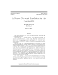
Distributed Diagnostics Tool for Sensor Networks
Master’s Thesis in the Master Degree Program, Network and Distributed
Systems
XINZHANG
Department of Computer Science and Engineering
CHALMERSUNIVERSITYOFTECHNOLOGY
Göteborg, Sweden, 2012
Master’s Thesis 2012
Distributed Diagnostics Tool for Sensor Networks
Master’s Thesis in the Master Degree Program, Network and
Distributed Systems
XIN ZHANG
Department of Computer Science and Engineering
CHALMERS UNIVERSITY OF TECHNOLOGY
Göteborg, Sweden, 2012
The Author grants to Chalmers University of Technology and University of
Gothenburg the non-exclusive right to publish the Work electronically and in a
non-commercial purpose make it accessible on the Internet. The Author warrants
that he/she is the author to the Work, and warrants that the Work does not contain
text, pictures or other material that violates copyright law.
The Author shall, when transferring the rights of the Work to a third party (for
example a publisher or a company), acknowledge the third party about this
agreement. If the Author has signed a copyright agreement with a third party
regarding the Work, the Author warrants hereby that he/she has obtained any
necessary permission from this third party to let Chalmers University of
Technology and University of Gothenburg store the Work electronically and make
it accessible on the Internet.
Distributed Diagnostics Tool for Sensor Networks
Master’s Thesis in the Master Degree Program, Network and distributed systems
XIN ZHANG
©XIN ZHANG, 2012
Examiner: Elad Michael Schiller
Department of Computer Science and Engineering
Chalmers University of Technology
SE-412 96 Göteborg,
Sweden
Telephone +46 (0) 31-772 1000
Göteborg, Sweden, 2012
Distributed Diagnostics Tool for Sensor Networks
Master’s Thesis in the Master Degree Program, Network and Distributed Systems
XIN ZHANG
Department of Computer Science and Engineering
Chalmers University of Technology
Abstract
Sensor network plays more and more import role in modern industries, but
debugging and diagnosis is always error-prone and time-consuming.This research
aims to make up the debugging gap between simulation and testbed on sensor net.
‘SUSE’ is a set of tools that provide a variable level debugging and diag-nostics
tools on both emulators and testbeds. Firstly, ‘Snapshot collector’ used to generate
snapshots on test beds then collect them into a sink node. Secondly
‘Up/Downloader' make helps on transferring data between emu-lators and test
beds. 'Standard mask generator' creates variable masks from snapshots. Finally
‘Evaluator’ generates a report depends on comparison between masks that come
from emulators and test beds.'SUSE' can fulfill the gap between simulations and
testbeds, which also provides help on performing different tests and fault injection
on testbeds. 'SUSE' is also a powerful idea that can be expanded to different
platforms.
Key words: Sensor Networks, Debug, Diagnose,’SUSE’, ‘Snapshot Collector’,
‘Up/Downloader', 'Standard Mask Generator', ‘Evaluator’.
2
Contents
CHAPTER 1 INTRODUCTION .................................................................................................................................... 1 1.1RELATED WORK ............................................................................................................................................................. 2 CHAPTER 2 PRELIMINARIES .................................................................................................................................... 4 2.1 TEST BED ....................................................................................................................................................................... 4 2.2 CONTIKI .......................................................................................................................................................................... 5 2.3 COOJA ............................................................................................................................................................................. 5 2.4 CHECKPOINT PROCESS .................................................................................................................................................. 6 2.5 TASK DEFINITION .......................................................................................................................................................... 7 CHAPTER 3 DESIGN STRATEGIES FOR DISTRIBUTED DIAGNOSTICS TOOL ............................................... 8 3.1 SNAPSHOTS COLLECTOR ................................................................................................................................................ 9 3.2 UP/DOWNLOADER ...................................................................................................................................................... 10 3.3 STANDARD MASK CREATOR ........................................................................................................................................ 10 3.4 EVALUATOR .................................................................................................................................................................. 13 CHAPTER 4 IMPLEMENTATION ............................................................................................................................ 14 4.1PLATFORM AND ACHITECTURE .................................................................................................................................... 14 4.2SNAPSHOTS COLLECTOR .............................................................................................................................................. 14 4.3 EVALUATOR .................................................................................................................................................................. 17 4.4UP/DOWNLOADER ....................................................................................................................................................... 17 4.5STANDARD MASK CREATOR PSEUDOCODE ................................................................................................................. 19 4.6DICTIONARY .................................................................................................................................................................. 20 4.7DIAGNOSE ...................................................................................................................................................................... 21 CHAPTER 5 EXPERIMENT AND EVALUATION ...................................................................................................... 22 5.1DESIGN .......................................................................................................................................................................... 22 5.1.1 CONFIGURATION .............................................................................................................................................................................. 22 5.1.2MICRO EVALUATION ........................................................................................................................................................................ 23 5.1.3MACRO EVALUATION ....................................................................................................................................................................... 24 5.2 MICRO EVALUATION .................................................................................................................................................... 25 5.2.1 TIME CONSUMPTION ANALYSIS .................................................................................................................................................... 26 5.2.1.1TIME CONSUMPTION FOR CHECKPOINT PROCESS .................................................................................................................. 27 5.2.1.2 TIME CONSUMPTION FOR DATA COLLECTION ....................................................................................................................... 28 5.2.1.3 TIME CONSUMPTION FOR FILE TRANSFER ............................................................................................................................. 29 5.2.1.4 TIME CONSUMPTION ANALYSIS ................................................................................................................................................ 30 5.2.1.5 DISCUSSION ................................................................................................................................................................................... 31 5.2.2CPUCONSUMPTION ................................................................................................................................................... 32 5.2.2.1 DISCUSSION ................................................................................................................................................................................... 33 5.2.3MEMORY CONSUMPTION .......................................................................................................................................... 34 5.2.3.1 DISCUSSION ................................................................................................................................................................................... 35 5.2.4 DISCUSSION FOR MICRO EVALUATION ........................................................................................................................................ 35 5.3MACRO EVALUATION .................................................................................................................................................... 35 5.3.1 DISCUSSION ....................................................................................................................................................................................... 37 3
6 DISCUSSION ................................................................................................................................................................ 38 BIBLLIOGRAPHY ......................................................................................................................................................... 39 APPENDIX A QUICK START ......................................................................................................................................... 40 A.1USAGE FOR ‘SNAPSHOTS COLLECTOR’ ......................................................................................................................... 40 A.2USAGE FOR ‘UP/DOWNLOADER’ ................................................................................................................................. 41 A.2.1 TRANSFER FROM COOJATO COMPUTER ...................................................................................................................................... 41 A.2.2 TRANSFER FROM COMPUTER TO COOJA ..................................................................................................................................... 42 A.2.3 TRANSFER FROM TESTBED TO COMPUTER ................................................................................................................................ 42 A.2.4TRANSFER FROM COMPUTER TO TESTBED ................................................................................................................................. 43 A.3USAGE FOR ‘STANDARD MASK CREATOR’ ................................................................................................................... 44 A.4USAGE FOR ‘EVALUATOR’ ............................................................................................................................................ 44 APPENDIX B USER MANUAL .................................................................................................................................. 45 B.1 BASIC USAGE OF COOJA ............................................................................................................................................... 45 B.2 NODE_ID BURNING ...................................................................................................................................................... 45 B.3 UPLOAD CODE .............................................................................................................................................................. 46 APPENDIX C SENSOR CODE ................................................................................................................................... 47 CHALMERS
Computer Science and Engineering Master Thesis 2012
4
5
List of Figures
FIGURE 3.1 Compositions of ‘SUSE’ FIGURE 3.2 Snapshots collector FIGURE 3.3 Checkpoint processes that run on multiple nodes FIGURE 3.4 Creation of a standard mask FIGURE 3.5 Working flow of evaluator FIGURE 5.1 Configuration of experiments FIGURE 5.2 Time consuming and the comparison between different numbers of nodes, it is obvious that time is positive correlation with numbers of nodes FIGURE 5.3 Time occupations on COOJA and Test bed, data collection and file transfer occupy the largest propotion of totally time consuming FIGURE 5.4 CPU consumptions for sink node and supplier nodes; it is clear that data collection is a CPU-­‐intensive process. FIGURE 5.5 ROM & RAM consumption, obviously checkpoint only use little memory space comparing with data collection FIGURE 5.6 A sample report CHALMERS Computer
Science and Engineering Master Thesis 2012
6
Glossary
Definitions
Contiki
Name of a micro-operating system.
Cooja
Name of a simulator inContiki.
Sink node
Node to receive checkpoint files from
others.
Supplier node
Node to send checkpoint file to sink node.
VANET
Vehicle ad-hoc networks.
CFS
Coffee File System
Tmote Sky
Name ofa sensor model.
CHALMERS Computer
Science and Engineering Master Thesis 2012
7
Chapter 1
Introduction
Recent work on sensor networks shows growing demands in debugging and
diagnosis. They need innovative applications to enhance diagnostics
performance and reduce the gap between simulator and test bed at the same time.
The prospects of these applications depend on the ablility of recording instant
snapshots from all nodes, and then transfer these snapshots between simulators,
computers and test beds. We consider a solution that may create, transfer
snapshots and then diagnose them. One of the options is the checkpoint function
that provided by Contiki, which can freeze a node and dump all memory content
into a checkpoint file (one snapshot).
The studied problem appears when sensor nodes can only rollback from where
the snapshots were created, and there is no diagnosis method that can help
developers from manually checking these snapshots, see Chapter 2. We propose
an integrated model that supports data transmission between simulator and test
bed; we also provide an efficient diagnosis method by evolving a variable mask,
see Chapter 3. Let us illustrate the problem and challenges of performing
diagnosis on sensor networks. Consider two neighboring nodes are working on
an algorithm, they work well in the first cycle, and then one node starts to
generate wrong data from the second cycle, but the strange thing is that this bug
is never produced on simulator. In the past, there are three options for us to settle
this dilemma: a regression test on another simulator, checks source code line by
line or analyzes the output. Alghough we can fix the bug sooner or later, but
apparently this is a very time comsuming process especially when we work on
large numbers of nodes.
-1-
8
1.1 Related Work
A number of diagnosis methods have beens used for sensor networks, for
example [1] consider diagnositic tracing for sensor networks,[2] studied fault
management in sensor networks, [3] consider monitoring and diagnosis in sensor
networks, [7] mention how to enabling efficient static verification, and [8, 9]
look into the problem of fault diagnosis and the discovery of silent failure in
sensor networks.Some of them have provided variable related diagnosis: for
example, [1] shows a inter-procedural and intra-procedural tracing on the values
of key variables, [10] studied a hybrid simulation and emulation on test bed of
VANETs. These are more efficient methods than before but they still do not
consider ‘cross-border’ diagnosis to fulfill the differences between simulator and
test bed.
Osterlind et al. [5] purposed a solution for a ‘cross-border’ diagnostic method by
transferring checkpoint files between simulator and test bed. This solution shows
a new thinking. Observe that this diagnostic method can reproduce bugs on
simulator after we found them in test bed. We can firstly dump all variables into
a checkpoint file on testbed, and then send these checkpoing files to simulator;
after rollback from these checkpoint files, we can restart the scenario that was
originally running on test bed and trace the variables if any of them have
triggered the bug on test bed. But this method still does not a complete solution.
One of the reasons is that there are over 500 or 600 variables in one sensor node
under normal circumstances, so manually validating all variables is a super time
consuming task although we can transfer and rollback all variables from test bed
to simulator through checkpoint files, just imagine what will happen if we have
to debug a 10-sensor system.
We note that an efficient diagnosis can display suspect variables from all nodes
and it should also work at least semi-automatically instead of fully manually
checking. Comparing with existing literature, our solution provides at least two
contributions: first of all, it provides a new kind of simulation that involves both
-2-
-9-
simulator and test bed. When comparing to our solution, other existing method
can only operate the simulation either on simulator or test bed, so they can not
deal with the bugs only produced on test bed but never show themselves on
simulator. Our advantage is obvious: we can reproduce the bugs on simulator
just after we found them on test bed. What’s more, we can carry on further
diagnosis by observing the values of variables. On the other hand, our
implementation provides a fast variable level diagnosis mechanism that can
automatically diagnose the suspect variables with possible faulty values within
tens of seconds; comparing with other existing methods, our solution can save a
lot of time when diagnose on systems that involves large number of sensor nodes.
-3-
-10-
Chapter 2
Preliminaries
The system consists of a test bed and a simulator. In this case, the test bed
consists of 3 sensor nodes and we use Cooja to work as the simulator. The tasks
of test bed are running algorithms then create and collect checkpoint files; and
the tasks of simulator is to perform diagnosis by generating masks and then find
out suspect variables by comparing them. From section 2.1, we will introduce
basic knowledges for test bed, Contiki, Cooja and checkpoint process. More
information could be found on the website of Contiki.
2.1 Test Bed
We use three Tmote Sky sensor nodes to work as test bed in this case. Tmote
Sky is a broadly used energy-saving wireless sensor, it also supports varies
standard ADC interfaces or SPI/I2C interfaces. Tmote Sky use MSP430 series
CPU and mostly commonly are F1161 and F5438; among them, F1161 has
lowest energy consuming feather in MSP430 series but its computing
performance is also much lower than F5438. MSP430 is able to make use of tool
chains that are provided by TI, but those tool chains cannot support full features
of this type of CPU. One advantage is that the Tmote sky sensor nodes supports
both Contiki and TinyOS embedded operating system. It also supports extremely
low power consumption and highly integrated antenna. Tmote Sky has become
an eco-friendly device, which also broadly used in many areas. In this case, we
use one Tmote Sky to works as sink node, which task is to receive checkpoint
files from all others.
-4-
-11-
2.2 Contiki
Contiki was developed by SICS (Swedish Institute of Computer Science).
Contiki has the advantage in supporting IP connections when comparing with
TinyOS. Although Contiki is a lightweight embedded operating system, but it
supports many enhanced features, such as multi-threading, build-in TCP/IP stack,
file system and even a web browser, which is maybe the smallest in the world.
Contiki is an open-source embedded operating system, and it is easy to
transplant to many sensor platforms. One of its advantages is it supports an
embedded file system named Coffee File System (CFS), which use external flash
as its storage media when comparing to other embedded systems. Observe that
Coffee File System can help delivering update files by transferring them to nodes’
external disk then trigger the update operation if we want to spread the new code
base to large amount of sensors. But it also comes with one disadvantage: it
cannot use either large-scale data structure or memory cache due to the limited
memory size when comparing to file systems that are using on computers.
Protothread is another advanced feature that provided by Contiki. Protothread is
a process controlling model, which is a lightweight threads mechanism and it can
run without the support of per-process stacks. On the other hand, protothread
does not have any complex state machines and full-featured multi-threading
operations, so it can fulfill the limited hardware requirement on sensors. One
disadvantage of protothread is the lack of support for local variables when we
switch context between threads or thread blocks, since Contiki does not has any
internal stacks to maintain variable states. Fortunately, we can define variables
into a ‘static’ type to avoid this.
2.3 Cooja
Cooja is a simulator and it is also a component of Contiki. Cooja can simulate
the operations of multiple sensors before we deploy them on test bed. It is a
multi-layer simulation tool, which can perform simulation on all three levels. But
-5-
-12-
it is also coming with a disadvantage: it cannot implement a simulation on all
three layers in one node simultaneously; so if we want to perform the simulation
on all levels in one scenario, we have to run it three times. This feature slightly
reduces the practical value to some extent.
Cooja provides us flexible expanded capacity with multiple plugins and
interfaces. Observe that plugins can be divided into five categories: mote plugin
can initiate from the menu of one specific node instead of Cooja’s menu. It
provides functions that are directly related with nodes, such as read/write motes’
memory, serial input/output and Contiki shell. Secondly, Contiki provides
simulation plugins that can be activated throughout one or multiple simulations.
It can be initiated from the Cooja’s menu. Thridly, Cooja plugins are general
plugins for all instances, and they do not depend on any senarios, such as the
control panel, simulation visualizer and the timeline. Simulation Standard plugin
is easy to confuse with simulation plugin, the only difference is that they can
initiated by default together with simulation initiating, what’s more, we can
configure them by editing configuration in Cooja. Lastly, Cooja standard plugins
can also automatically activated with simulation initiating simultaneously.
One advantage of Cooja is that we can develop plugins that we need, and then
add them into plugin list before using them in a new session.
2.4 Checkpoint Process
Checkpoint process works in Tmote Sky nodes, which dumps all content from
memory to a checkpoint file. This is a useful feature when we diagnose on
simulator or test bed; we can rollback from them and let the nodes go backwards
to previous states when we have created them.
Observe that there is one factor that might restrict the effect of checkpoint
mechanism: checkpoint files can only rollback in same environments where we
have created them.Contiki does not provide any tools that can transfer
checkpoint files between simulator and test bed.But obviously it will be more
-6-
-13-
powerful if we can.Other than that, although we can rollback from a checkpoint
file, we have to manually check the variables when a bug occurs.
2.5 Task Definition
The problem of diagnosis on sensor networks is that we need a tool, which can
enhance the efficiency of testing and debugging when we deploy our source
code from simulator to test bed. This tool should provide the ability to make
snapshots on nodes, transfer them between simulator and test bed, and then
perform diagnosis on them.
-7-
-14-
Chapter 3
Design Strategies for Distributed
Diagnostics Tool
We have addressed four problems in the design of diagnostics tool: collect
checkpoint files to sink node; transfer checkpoint files between sink node and
computer; generate standard masks; perform an automatically diagnosis and
figure out all possible faulty variables. Before settling implementation details in
Chapter 4, we organize all functions into four low coupling and high cohesion
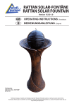
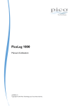
modules according to the problems that we have addresses, see figure 2.1.
Snapshots
collector
Standard Mask
Generator
Evaluator
Up/
Downloader
Compositions for ‘SUSE’,‘S’ is the first letter of ‘Snapshots
collector’, ‘U’ is the first letter of ‘Up/Down loader’, ‘S’ is
the first letter of ‘Standard mask creator’, ‘E’ is the first
letter of ‘Evaluator’, that’s why we call it: ‘SUSE’.
Figure 3.1 compositions of ‘SUSE’
-8-
-15-
‘Snapshots collector’ creates checkpoint files and collects them to sink node;
‘Up/downloader’ exchanges files between sensors (both in simulator and test
bed) and computers. ‘Standard mask creator’ creates a standard mask, which
works as a reference. And finally, ‘Evaluator’performs diagnosis by comparing
target masks and a standard mask. We present the design details for different
modules from section 3.1.
3.1 Snapshots Collector
This module creates and collects checkpoint files to sink node. Theoretically,
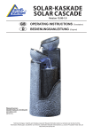
‘Snapshots Collector’ is consists of three main procedures: an algorithm that is
going to be diagnosed, a process that creates checkpoint files and a datacollection process.
Main
Process
Sample
algorithms
Snapshot
Data
collection
Files download
to PC
Timer
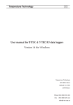
Figure 3.2Snapshots collector
Let us look into a typical workflow of ‘Snapshots Collector’, see figure 2.2.
Given one algorithm that runs periodically on test bed, we say that this algorithm
is the target for diagnosing. Observe that figure 2.2 shows only one cycle within
a loop; the sample algorithm then follows by a checkpoint process, which saves
all variables from memory to a checkpoint file.As soon as the checkpoint
process is finished, we start a collect protocol in order to collect checkpoint files
to sink node. This process includes a parent finding algorithm and a routing
algorithm by default, and it costs about 30 seconds to discover the routing
information before data transfer. After that, we pad data into radio packet and
send them through a radio connection to sink node.In this case, one sink node
has the capability to save 100 snapshots at the same time.Other than this, we
setup a 20 seconds delay for file transfer from Cooja/test bed to
computers.Observe that one of the advantages of ‘Snapshots Collector’is
simpleto use: we simply replace the sample algorithm to another that we want to
debug. In next section, we present standard mask creator that works as a
reference in diagnosis.
-9-
-16-
3.2 Up/Downloader
Up/downloader exchanges checkpoint files between test beds and simulators.
Cooja has provided a socket serverfor sending and receiving files, but we have
to develop a client that works on computer. Considering test beds are connected
to computer through a serial port, we develop a serial reader and writer for
exchanging files between them.
Contiki does not provide any commands that directly write data to serial ports,
but we have found a uart_writeb ()function in serial driver, which sends one byte
to serial port at each time.According to receive data in nodes, let us look into a
typical receiving workflow in Contiki,as soon as we send a byte to nodes,
Contiki calls an input handler function and then sends the byte to a receiving
buffer.So in this case,we redefine the input handler and redirect the incoming
data flow when we receive files in nodes.
One important thing to also note is that the writing speed in nodes is much
slower than reading, so we define a buffer and transfer files by blocks in order to
enhance the writing performance.
3.3 Standard Mask Creator
This module creates standard masks to work as references in debugging.
Observe that a standard mask indicates which variable is modified during
checkpoint process and which isn’t. This provides the ability to compare
between a standard mask and target masks; the latter is a mask comes from test
bed that needs to be diagnosed. Let us look into a distributed sensor neworks to
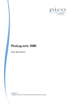
find out what happens when we create checkpoints.When we trigger a
checkpoint process on all nodes, they do not start at same time. There are two
possible reasons that may explain this, one is we do not have any synchronize
mechanism on nodes, and the other is that nodesmust react to interrupts or
-10-
-17-
incoming packets before they start checkpointing. We can observe schematic
diagram from figure 2.3.
Stop at
9400ms
Start
Stop at
9700ms
Node 1
Start
Stop at
10000ms
Node 2
Node 3
Totally time for all nodes: 10000ms
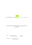
Figure 3.3Checkpoint processesthat run on multiple nodes
We have worked out a solution to combat the asynchronous problem during
checkpoint process. Recall from the previous paragraphs that in order to find out
which variable has been modified, we need to devide checkpoint process into
several snapshots then compare between them. See figure 2.4-up, in this case,
we cover all checkpoint process from all nodes by defining an earlier start time
and a later end time on them.
-11-
-18-
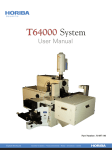
Snapshot1 Snapshot2 Snapshot3 Snapshot4 Snapshot5 Snapshot6
Variable N
Equals?
... ... ... ... ...
Equals?
... ... ... ... ...
Equals?
Equals?
... ... ... ... ... ... ... ... ... ...
Equals?
... ... ... ... ...
Snapshot7
Equals?
... ... ... ... ...
Start
Stop
Totally time for all nodes: 10000ms
Sometime Before
Sometime After
First Step: Create One Mask in Cooja
Data source: Given one node, define several breakpoints in checkpoint
process and create snapshots from it. Then save all snapshots into database.
Operation: Compare each variable from the first snapshot to the last, keep
their value if they equal to each other, modify to a special value if they don’t.
Checkpoint file
Variable N
Checkpoint file
... ... ... ... ...
Equals?
... ... ... ... ...
Node 1
Checkpoint file
Equals?
... ... ... ... ... ... ... ... ... ...
... ... ... ... ...
Node 3
Node 2
Checkpoint file
Equals?
... ... ... ... ...
Node 4
Step 2: Create One Mask from Test bed
Data source: Given all nodes in test bed, create one checkpoint file in each.
Variable N
... ... ... ... ...
Mask from Cooja
Equals?
... ... ... ... ...
Mask from test bed
Step 3: Create One Standard Mask
Operation: Import all checkpoint files into Cooja, then compare each variable
from the first checkpoint file to the last, keep their value if they equal to each
other, and modify to a special value if they don’t.
Data source: One mask comes from Cooja and one comes from test bed.
Operation: Compare each variable between them, keep their value if they
equal to each other, modify to a special value if they do not.
-12-
-19-
Figure 3.4 Creation of a standard mask
Figure 2.4-middle shows the creation of a mask from Cooja. It is not a standard
mask unless we amend it by a mask that comes from test bed. We cannot
interrupt nodes when they are running, but we can create mask from their
checkpoint files, because a checkpoint file copys all variables from memory.In
figure 2.4-down,we amend the Cooja mask in order to generate a standard
mask.Next step, in section 3.4, we perform a diagnosis with the help of
evaluator.
3.4 Evaluator
Evaluator performs comparison between different masks, and then generates a
report to display all suspect variables, together with their physical addresses.
Create Standard
mask in cooja
File upload
to cooja
Create
Mask
Rollback
Compare
Mask
Report
Figure 3.5Working flow of evaluator
This module is based on the ability to make comparison between different
masks. Observe from figure 2.5 that we need to upload checkpoint files to Cooja
in order to create debug mask. A debug mask is similar with test bed mask that
has been mentioned in section 3.3, the only difference is, we use checkpoint files
that come from a faulty test bedthat needs to be diagnosed.If there are any
differences between a debug mask and standard mask, we save these suspect
variables into final report together with their physical addresses.
-13-
-20-
Chapter 4
Implementation
This chapter delineates the challenges and techniques that related to the
implementation of ‘SUSE’, such as: Contiki does not provide a bulk data
transmission protocol between different sensors, so we have to find a method in
order to collect checkpoint files to sink node. Other than this, we have to
develop a tool to transfer different checkpoint files between sink and computer.
We also have to find out how to define a standard mask and how to implement
the fast diagnosis automatically.
4.1 Platform and Achitecture
For all implementations and evaluations in this case, we use Contiki2.5 and
Tmote sky to work as operating system and test bed; the latter is based on an
MSP430 with 802.15.4 compatible CC2420 radio chip. Tmote sky provides a
one-megabyte external flash storage memory (ST M25P80 40MHz) and two
light sensors. Tmote sky also includes a 10k byte RAM and a 48k byte flash.
4.2 Snapshots Collector
The data colleting protocol is initially designed for gathering data from sensors
such as temperature, humidity or light, but it supports packet size up to 100
bytes. In this case, we collect files by selecting an appropriate packet size,
transmission interval and retransmission time.
-14-
-21-
1
collect_open();
// open collect channel
2
collect_find_sinknode();
// find sink node through a routing algorithm
3
memcpy(packet_buffer);
//read data from file then pad into rime packet
4
collect_send();
5
packet_buffer_clear(); // clear the rime buffer and wait for new data
// send out packets through collect channel
In this case, we tweak the performace of data collection by modifying time
interval and retransmission time between each two packets. If we decrease these
two settings, we enhance the data-collection performance but also increase the
data loss rate at the same time. Next, we will describe the implementation of
data collection on sink node and supplier nodes.
Implementation of sink node in data collection:
// Variables definition
1
collect_open ();
// define and open a new collect channel
2
if (node_id==1){
// judge whether it is the sink node by node id
3
collect_set_sink ();
// if this is sink, setup collect protocol by it
4
}
Sink node is chosen by node id, and then other nodes find sink node by a parent
finding algorithm, which also works as a simple routing method. Next is the
receiving method of sink node.
1
cfs_open ();
// define a file for incoming checkpoint files
2
memcpy (packetbuf);
// receive packets and then copy to a buffer
3
cfs_write ();
// save data from buffer to a file
4
cfs_close ();
// close the file after each writing
-15-
-22-
We save data into different files since all received packets are distinguished by
their rime addresses in headers. Sink node also transfers files with computer, see
section 4.4 for more details on file up/download.
Implementation of supplier nodes in data collection:
1
collect_open ();
// define and open a new collect channel
2
if (node_id! =1)
// make checkpoint on other nodes instead of sink
node
3
{
4
make snapshot;
5
}
6
collect_parent ();
// find sink node
7
setup etimer ();
// an event time for time interval between two
packets
8
if (checkpoint file exists)
9
{
10 read file;
// if checkpoint file exists, goto next step
//read from checkpoint files, read 64 bytes in
each time
11 memcpy (packet_buffer);
// pad data into packet buffer
12 send out packet ();
// send packets to sink node
13 packet_buffer_clear ();
// clear packet buffer for next transimission
14 }
15 cfs_close ();
// close checkpoint files
We divide checkpoint files into blocks for data collection, and we select 64 bytes
as the block size when considering both rime buffer and collecting efficiency.
We also clear the packet buffer after each sending and then wait for new
data.One important thing to also note is that there is no synchronization
mechanism for both senders and receiver. At the end of data collection, we setup
a 20 seconds delay for file transfer from Cooja/test bed to computer.
-16-
-23-
4.3 Evaluator
Let us look into an evaluator to find out its implementation, we use database to
save and excute large scale of data.In this case, each node creates500~600
varaibles in their snapshots, suppose each mask needs 20 snapshots from 2
sensors, then we have to deal with 20,000 to 24,000 variables. This is why we
decided to use database instead of other options.
MySQL is an open-source, relational database manages system, which is
relatively lightweight than others such as SQL server or ORACLE. MySQL also
provide several client-end tools, take MySQL administrator as an example, it
provides an integrated interface for database management. Other than that, it
provides a MySQL query tool that can execute SQL query statements.All of
these features help us to manage and execute data efficiently.In this case, we
need to download a java connector that works as the bridge between MySQL
and Cooja, after that, we define SQL statements and execute them.See section
4.5 for more details about mask creation.
4.4Up/Downloader
Recall from Chapter 3 that the writing speed of flash file system in MSP430 is
much slower than RAM or ROM. And considering the potential writing latency
between any two bytes, we decide to use a blocked transfer. So we define an
internal buffer, which can receive bytes through UART then write to flash as a
block.Then it is possible to transfer blocks in a much faster speed then wait for a
short latency between each two.
-17-
-24-
1
FILE *fp = fopen (checkpoint file);
2
while (1) {
4
for (bytes<64){
//open checkpoint file from hard disk
// read 64 bytes from file
5
sleep ();
// define a short time interval
6
write (serial ports);
// write data to serial port
7
}
8
usleep (longer interval);
// a longer interval between each two 64
bytes
9
}
Cooja simulates sensor’s serial ports into standard socket ports. Each mote that
simulated in Cooja has been assigned a unique port number consists by
“60000+node id”. Then we call the uart_writeb (byte) function from motes in order
to send bytes tothe socket client that runs on a computer.Checkpoint files are
savedas byte files, the name format is designed as: Snapshot_hour-minutesecond.bin. The file should always use a expansion name as '. bin’, which is the
default type for byte files in Ubuntu.
-18-
-25-
4.5 Standard Mask Creator Pseudocode
Create a mask from Cooja:
1
SELECT * from snapshots table where VarName='first variable' and id not in
(select min (id) from mask group by VarName having count (*)>1) limit 1
//firstly find all records that with same variables’ name, start from the first variable
2
TRUNCATEtarget table
//clear
target table
3
SELECT* from snapshots table where VarName='first variable'
//select
first variable from table that evolve all snapshots
4
TRUNCATEtable temp table
//clear
temp table
5
SELECT* from snapshots where id=?
//traverse
all variables by selecting from first to last variable
6
INSERTinto temp table select * from mask where VarName=? order by desc
//select data items into temp table, which has same variable name
7
SHOWtable status of temp table
//count the
length of temp table, which is also the number of baches of data.
8
SELECTValue from temp table order by id asc limit 1
// find the
value of first variable when listing by ascending
9
SELECTValue from temp table order by id desc limit 1
// find the
value of first variable when listing by descending
10 INSERTignore into target table select * from temp table order by id asc limit
1
//if they
are same, then variables that come from all batches has same data value, then insert to
the target table.
11
UPDATEtemp table SET value= -99999 order by id asc limit 1
//else,
mark the value.
12 INSERTignore into target table select * from temp table order by id asc limit
1
//insert the marked variable into target table.
-19-26-
Create a standard mask:
1
SHOW table status from mysql like 'test bed mask'
// find
table length of test bed mask to ensure the length of loop
2
SELECT * from test bed mask where VarName='first varaible'
//traverse
all variables in test bed mask from start to end.
3
TRUNCATE table temp table
//clear
temp table
4
SELECT * from test bed mask where id=?
//select
variables from first to end
5
INSERT into temp table select * from test bed mask where Varname=?
//select variables into temp table from test bed mask
6
INSERT ignore into temp table select * from Cooja mask where Varname=?
//select variables into temp table from COOJA mask
7
SELECT Value from temp table order by id asc limit 1
// find the
value of first variable when listing by ascending
8
SELECT Value from temp table order by id desc limit 1
// find the
value of first variable when listing by descending
9
INSERT ignore into standard mask select * from temp table order by id asc
limit 1
//if they equals with each other, then insert into final table.
10 UPDATE temp table SET value= special value order by id asc limit
1//otherwise mark the variable with a special value
11
INSERT ignore into standard mask select * from temp table order by id asc
limit 1
//insert the marked variable into target table
4.6 Dictionary
Dictionary is a mapping between variables and their addresses. We build the
mapping by retrieving data from Coojabecauseitalways createsanew mapping
between memory elements and their addresses when it generates new nodes.
Generally speaking, we can build a dictionary in two steps: (1) Read variables
-20-27-
names through the memory object, and (2) Traverse all variable names then
retrieve their physical address through a ‘get address’ method in Cooja, then
save them into database.Now if we found any problems during diagnosis on test
bed, it is possible to knowtheir name through their physical addresses or vice
versa.
4.7Diagnose
Diagnosis is a comparison between standard mask and a mask that needs to
debug. If variables have same value, remains. Then if variables have different
values, but one of their values has been marked that shows this variable can be
ignored, then keep the original marks. Otherwise marks the variable to a special
value. Finally we search in dictionary to find their physical addresses.
-21-28-
1
TRUNCATE table temp table
//clear temp report
table
2
SHOW table status from mysql like data table
//find length of
masks
3
SELECT * from data table where VarName=first variable //traverse
variables from 1st to end.
4
TRUNCATEtemp table
//clear temp table.
5
SELECT * from data table where id=?
//start from first
variable
6
INSERT into temp table select * from data table where Varname=? //select
data from debug mask
7
INSERT ignore into temp table select * from diagnose report where
Varname=?
//select data from standard mask
8
SELECT Value from temp table order by id asc limit 1
// find the value of
first variable when listing by ascending
9
SELECT Value from temp table order by id desc limit 1
// find the value of
first variable when listing by descending
10 INSERT ignore into tempreport select * from temptable order by id asc limit 1
//select
first value from temp table to temp report listing by ascending
11
INSERT ignore into tempreport select * from temptable order by id desc limit
1
//select
first value from temp table to temp report listing by descending
12 UPDATE temptable SET value= mark order by id asc limit 1
//mark
abnormal variables
13 INSERT ignore into tempreport select * from temptable order by id asc limit 1
//insert to
temp report
14 TRUNCATE table reporttemp
//clear temp report
15 TRUNCATE table diagnose report
//clear report
16 INSERT reporttemp select * from tempreport INNER JOIN dictionary ON
tempreport.VarName=dictionary.VariableName
//select data from
both temp report and dictionary
17 INSERT report SELECT id,SnapName,VariableName,Value,Addr FROM
reporttemp where Value=-1234567
//create report that evolves
physical addresses
-22-
-29-
Chapter 5
Experiment and Evaluation
We will introduce the experiments and evaluation of ‘SUSE’ in this chapter. We
test our design on a test bed that consists of 3 sensors, and we cover both micro
and macro evaluations, then we observe resources consumption and overall
characteristics. We can conclude from the evaluation that ‘SUSE’ can finish the
diagnosis within 9 minutes on testbed and it occupies the RAM and ROM in a
reasonable way. We will show and discuss more details from section 5.1.
5.1Design
5.1.1 Configuration
In this section we listboth hardware and software configurations in order to
describe the running environment for all experiments in this chapter.
Items Information Sensors: Tmote sky Sensor model MTM-­‐CM5000MSP CPU MSP430 RAM 10K bytes Flash 1024K bytes Contiki Version 2.5 Computer: UBUNTU 10.04 Operation system Compiling environment: GCC 3.8.3 JAVA 6 Table 5.1 Configurations of experiments
-23-
-30-
For all evaluations in this research we use three Tmote sky (MTMCM5000MSP)sensors that connect to a laptop through anUSB hub. Thus we can
upload source code to all sensors simultaneously instead of one by one. The
Contiki that we are using is running on a UBUNTU 10.04 instead of an instant
Contiki, one of the advantages is faster execution.
5.1.2Micro Evaluation
We firstly introduce our test planfor micro level benchmarkin this section.We
measure performance in different part of ‘SUSE’. These measurements includes
time consumption, CPU usage and storage analysis. Micro evaluation helps us to
determine the speed and effectiveness of ‘SUSE’. It can also help us to locate the
possible
bottleneck, which can possibly be improved. Take the time evaluation as an
example,wemeasure how much time does ‘SUSE’ needs on:(1) checkpoint
process,(2) data collection process and (3) file transferbetween sensors (both
working in Cooja andtest bed)and computer. We finish the timeworkby
calculating time difference between two watchpoints, whichhave been predefined in source code. Then we compare time usage between different parts of
‘SUSE’ and time usage between different numbers of sensor nodes in section
5.2.1.In section 5.2.2, we benchmark CPU consumption,whichis measuredby
CPU cycles that can read from‘MSP cycle watcher’inCooja. Another aspect that
we have measured is storage consumption,which is especially useful before
uploading code to test bed.In this case, we use ‘size –A’ command to benchmark
storage usage, ‘size –A’ is a build-in command in ‘MSP430-gcc’ compiler,
which analyzes memory consumption from compiled souce code, and then
display information on the screen.
One of the disadvantages to micro evaluation is manual execution; we have to
define watchpoints manually then copy data into aMicrosoft excel file for
creating charts.So maybe we can improve it to an automatically test frame.One
important thing to also note is that we did not benchmark power consumption in
this research. Power consumption is one of the key features for sensors that
-24-
-31-
working in natural environment, but ‘SUSE’ works in testing environment only,
so power measurement did not take into consider now.
5.1.3Macro Evaluation
In this section, we describe test plan for macro evaluation. Weimplement a
scenario on how to debug another algorithm with ‘SUSE’. This evaluation is
more like a macroscopic acceptance test and we find out whether ‘SUSE’can
fulfill our requirements, which has been described in previous chapters. In order
to perform the macro evaluation, firsly we have to introduce a sample algorithm
and this algorithm works as adebugging target. In this case, we develop a
simplified Dijkstra’s algorithm, Dijkstra’s algorithm is a self-stabilize algorithm
that firstly introduced in seminar paper of Edsger Dijkstra in 1974; this
algorithm quickly becomes the important foundation of self-managing computer
system and fault-tolerance computing system. One of the advantages is it does
need any strong assumptions comparing to previous algorithms.
In this research, it works on a three-sensor system: one sink node and two
working nodes that come into a stabilizedstate (one of them works as a
deterministic leader). They use numbers to represent their states, and theyinitiate
from two random states, then after several cycles of running, they come into a
consistent state and keep this state in the following time.
To test the ‘SUSE’ further, we plan to find out two answers from macro
evaluation: (1)whether ‘SUSE’ can successfully diagnose on other algorithms
and (2)whether ‘SUSE’ affect other algorithms during the diagnosis.In order to
answer the first question, we have to perform a complete test, then study and
discuss the diagnose report andvalidate whether ‘SUSE’ can distinguish between
a suspect variable and a correct variable but always changes its value. In order to
answer the second question, we print sensor’s state on screen and check their
correctness.One of the advantages to our macro evaluation is its practically,
because we can check whether‘SUSE’ works in a real scenario, which is
-25-
-32-
specially import for our research. But one of the disadvantages to our test is, we
cannottest it in all possible contexts, thus we cannot ensure that ‘SUSE’ can
diagnose all type of algorithms. To combat this, it is better to use it together with
other debug tools, such as a semantic checker or a GDB debugger.
In this research, we cover both micro and macro evaluation, or in another words,
both performance benchmark and acceptance test. One of the disadvantages in
our design is, we do not evolve other testing techniques such as memory leak
test, security validation or load test.Section 5.2 describes and discusses the micro
evaluation, section 5.3describes the conclusion of macro evaluation.
5.2 Micro Evaluation
5.2.1 Time Consumption Analysis
In this case, we perform time benchmarkfor three processes: checkpoint process,
data collection process and file transfer, because these processes are key
functions in ‘SUSE’. Other than this, time usage varies when running ‘SUSE’ on
different numbers of sensor nodes. We found that the best way to get accurate
validations is to compare time consumption between different settings. There are
many possible reasons for extra time consumption:an interfered radio
connection,data collection between two sensors in a long physical distance, data
loss during radio transimission, sender sendspackets in a much faster speed than
receiver can handle or even any random unknown reasons. This is why we
measure time usagefor ‘SUSE’; we have to state that although we are facing so
many uncertainties, ‘SUSE’ can still execute in a reasonable time range.
For all micro-evaluation we directly use two build-in tools to perform
benchmark in Cooja. One of them named ‘MSP code watcher’ and the other
named ‘MSP cycle watcher’. ‘MSP code watcher’ is a plugin that inserts
watchpoints in source code and then stop running on triggered watchpoints. This
is especially useful on our timework; we measure any time difference after the
definition of watchpoints. ‘MSP cycle watcher’ is a plugin that enable cycle
counting of CPU, so when use it together with ‘MSP code
-26-
-33-
watcher’; we have the capability to benchmark CPU usage between any two
watchpoints. These two plugins make it possible to perform micro evaluation,
taking advantage of its high accuracy.
In this research, we perform time benchmark in three steps: (1) first,we start
‘MSP code watcher’ andfind out the interesting part that we measure, then
define watchpoints to mark them in source code. (2) Second, we start the
simulation and save all timing information in an excel file when the simulation
reaches pre-defined watchpoints. (3) Last, we finish the timework in excel and
then generate charts. Next, we discuss time consumption for different process in
section 5.2.1.1-5.2.1.3; then analyze the overall timing ratio in 5.2.1.4; finally
Hundreds seconds we start a briefly discussion for time benchmark.
4.5 4 3.5 3 3 nodes(include one sink) 2.5 2 4 nodes(include one sink) 1.5 1 5 nodes(include one sink) 0.5 0 checkpoint data download collection from testbeds Figure5.2Time consuming and the comparison between different numbers of nodes,
it is obvious that time is positive correlation with numbers of nodes
5.2.1.1Time Consumption for Checkpoint Process
In this section, we discuss time benchmark for checkpoint process. As mentioned
before, when we make checkpoint files on several sensor nodes, they won’t
start/end at same time, because there isn’t any synchronization between them,
this is why we perform measurement on average time consumption.
-27-
-34-
We have compared the time benchmark between 3-5 nodes, and figure 8 clealy
shows that checkpoint process does not vary much. One of the possible reasons
is that they won’t interfere by external aspects. We can read from the figure that,
very little time difference between different numbers of sensors: only 0.301
seconds between 2 and 3
nodes, and 0.045 seconds different between 3 and 4 nodes.Comparing with the
totally operating time of ‘SUSE’, time usage for checkpoint (with two nodes) is
4.4% when operate in Coojaand 2.1% when operate on test bed. In this case, this
result is totally acceptable.
One important thing to also note is that the time usage for checkpoint process
different between Coojaand test bedwhen we increase the numbers of nodes.
Each sensor makes its own checkpoint on test bed and won’t affect others, but in
Cooja,all sensors share the same hardware resource. So imagine that if we run
checkpoint process on 1000 sensor nodes in Cooja, they have to use much longer
time than now. But when we compare time benchmark with data collection and
file transfer, we find that those two processes are greatly affected by numbers of
nodes.
5.2.1.2 Time Consumption for Data Collection
In this section, we discuss time usage for data collection process. We have
already known that data collection is both a CPU-intensive and radio-intensive
process. So we have to find out whether it can finish its job within a reasonable
time range. We perform benchmark between different numbers of nodes, and
then make a brief discuss on that.
We have clealy find out that data collection consumes a lot of time during
diagnose, and time varies a lot when running on different numbers of nodes. As
figure 8 shows, when we run data collection on three nodes, with one sink node
and two supplier nodes, it uses198 seconds to finish all data transfer; the time
-28-
-35-
increases to 218 seconds when we run the same process on 4 nodes; at last, data
transfer time increases to 403 seconds for a 5-node. Thetime interval
settingbetween each two packets is1 second in 3-sensor and 4-sensor system;
senders canretransmit onceif theydo not receive anyacknowledgment from sink
node. Thisdefinition isalmost the fastest settings for data collecting protocol. It is
obvious that the time consumption increasealong with the increasing of
nodes.Data shows the time interval should increase to at least 2 seconds in the 5sensor system.
This result shows that the data collect protocol finishesits job within a
reasonable time limit, but still not good enough. This is also one of the
disadvantages when we decide to use this protocol. To combat this, we can
implement a better data collect protocol in the future. But things are never
absolute; an off-the-shelf option can save a large amount of time from
developing and testing a new protocol.
5.2.1.3 Time Consumption for File Transfer
In this section, we discuss the benchmark result for file transfer. Firstly we need
to know that checkpoint files have to be transported between sensors (running in
Coojaor test bed) and computer in order to finish the diagnosis. File transfer
means serial port operation or system bus operation, they are all time consuming
jobs.
In this case we focus on pure transmit time only, and we decide to ignore other
operations such as shell input.We can read from figure 8 thatfile transfer with
Cooja does not waste too much time. One of the possible reasons is that, when
we upload/download files between harddisks and simulator, most jobsaredone
inside a computer system. Take this evaluation as an example, it only use 3
seconds to download single checkpoint file to hard disk from Cooja. And the
uploading time is 14 seconds, which is little longer but still fast enough.
However, it is little different when uploading to test bed, this operation costs at
least 900 seconds to upload a singlefile. One of the explaination is that the
-29-
-36-
continuous writing speed in Tmote sky is quite slow then reading speed. To
combat this, we have implementa self-defined internal buffer to optimize the
upload speed. The working procedure is: after we receive every 64 bytes in a
relatively fast speed, then write them into flash file within a little longer time
interval (500millisecond in this case). Finally, with the help of internal buffer,
we have successfully decreased the uploading time from 900 seconds to 270
seconds.
It is possible to tweak the size of internal buffer according to the specific
circumstances. Larger buffer can bring a faster transfer speed, but it consumes
more memory spaces. So if we debug a tiny program, it issafe to increase the
buffer size to 128 or even 256 bytes, but when we talk about normal
situations,64 bytes is still anappropriate buffersize. One important thing to also
note that upload to test bed is not commonly used in ‘SUSE’, because we
actually create masks in Cooja instead of test bed.
5.2.1.4 Time Consumption Analysis
In this section, we discuss the overall statistics of time occupation in ‘SUSE’.
This analysis clearly tell us which part is consuming large amount of time, and
also which part should be optimized if we decide to enhance system’s
performance.We separately discuss two situations: time statistics on Cooja and
time statistics on test bed.
Time(s) Time(s) initilize initilize sample broadcast checkpoint data collection -30-
-37-
sample broadcast Figure 5.3Time occupations on Cooja and Test bed, data collection and file
transfer occupy the largest propotion of totally time consuming
We read from the figure that most of the time is consumed by data collection
process when we perform the simulation in Cooja; data collection occupies
82.2% of total execution time, while sample algorithm only cost 1.7%. We have
calculated that the time usage of data collection is 50 times than sample
algorithm and 9.5 times than checkpoint process.When we study the result ontest
bed, we find that the time consumption for uploading files occupies even a larger
proportion. Relatively, file upload use 54% of the totally execution time and data
collection use about 39.8%.When we measure the overall time consumption, we
find that it costs 240 seconds to execute ‘SUSE’ from beginning to the end on
Cooja, and 497 seconds when running on test bed.
This evaluation clearly shows that, if we want to optimize the performance of
‘SUSE’, we should firstly consider about a new data collecting protocol, this is
good idea to enhance the performance on both simulator and test bed. Secondly,
it is obvious that we should speedup the file uploading speed to test bed, this is
especially important when we run ‘SUSE’ on large numbers of nodes.
5.2.1.5 Discussion
In this evaluation, we have so far been unsuccessful in finding any resources that
discuss the usage of time.Since ‘SUSE’ is an application for diagnose, despite
any detailed benchmark, 5 minutes is still a good evaluation result for it. We can
imagine that in the past, it is difficult to find a ‘wrong’ variable when a bug
occurs, or even if we can, we have to consume a lot of time on it. But now, with
the help of ‘SUSE’, we just use 5 minutes to find out all suspect variables from
test bed. This is a tremendous progress when comparing to the past.
One important thing to also mention, performance is a balance between speed
and stability. Firstly it is unrealistic to boost the performance infinitely, and then
we do not want to lose any packet when weenhance the performance. So if there
is any tweaking on time interval or transfer speed, it should follow by large
amount of stability test.
-31-38-
5.2.2CPUConsumption
In this section, we perform measurements onCPU consumption of ‘SUSE’.We
benchmark CPU load on three processes: (1) only sample algorithm, (2) run
sample algorithm and checkpoint process and (3) run all three processes
including data collection.
CPU load is a key feature when we talk about execution efficiency and power
saving.In this case, we evaluate the CPU load by counting CPU cycles.Each
microinstruction costs one CPU cycle on Tmote Sky,so if a program leads a
higher CPU cycling, it uses more time to finish the execution and it also
Ten million cycles consumes more electricity.
1.2 1 0.8 CPU consumption-­‐-­‐sink node 0.6 CPU consumption-­‐-­‐
other nodes 0.4 0.2 0 without both with checkpoint with both Figure 5.4CPU consumptionsof sink node and supplier nodes, it is clear that data
collection is a CPU-intensive process.
In this case, we use both ‘MSP cycle watcher’ and ‘MSP code watcher’to
benchmark CPU counting in Cooja. Then we copy and save all data into an excel
file.We read from figure 10 that it is does not consumea lot CPU cycling when
we only run sample algorithm on test bed.Sink node uses 1.9227201(million)
cycles to finish this algorithm and the other two nodes use 1.7050251(million) to
finish their job.CPU counting becomes higher when we run both sample
algorithm and checkpoint process. In this case, supplier nodesuse 8.2083616
(million) cycles to finish both porcesses, we can calculate that it is about 4.8
times when comparing to the previous benchmark.It is obvious that
-32-
-39-
data collection process uses largest amount of CPU performance. Supplier nodes
use 105.8424274 (million) cycles to finish all three processes, this data is almost
62times of sample algorithm. The situation is similar when we evaluate it on
sink node, which uses106.060114 (million) cycles for all three processes.
5.2.2.1 Discussion
In this case, we find that CPU consumption differs a little between sink node and
a supplier node, one of the possible reasons is they execute different part of
source code. Take the sink node as an example, it does not run sample
algorithms and checkpoint process but it receives data from both supplier nodes
during data collection. On the other side, supplier nodes simply send out packets
but they might need more CPU cycling during checkpoint process and parent
finding. But generally speaking, both sink node and supplier nodes use similar
CPU costage in all three comparisons. We also find out that sink node costs little
more cycling during data collection, one of the possible reasons is supplier nodes
operate CFS file (read operation) once in each loop, but sink node operates CFS
file twice (write operation).Because of this, sink node consumes 12.77% cycles
more than supplier nodes when we run sample algorithms only, and the ratio
decrease to 2.6% when we running both sample algorithm and checkpoint
process. When we compare the totally execution, we find that sink node costs
only 0.2% more than supplier nodes.
We also found out that the CPU usage remains the same number when we run
same processes.This is reasonable result because each instruction should use a
fixed number of CPU cycles.On the other hand, this is also one of the
advantages of our method, which means that we have retrieved data correctly
from Cooja.
-33-
-40-
5.2.3Memory Consumption
In this section, we carry out the benchmark for memeory usage.We evaluate how
much memory that has beenusedby ‘SUSE’ in both RAM and ROM. For Tmote
sky nodes, variables are stored in RAM andsource codesaved in ROM. This
evaluation is especially important to sensor network because memory efficiency
is always a key feature to consider. In this case,we use a ‘size -A’ command to
measure memory usage; ‘size -A’ is a build-in command from MSP430-gcc
compiler and it can calculate memory occupation from compiled source file.
Other than this, we compare both RAM and ROM consumption from three
aspects: (1) when we only run sample algorithm; (2) when we run both sample
algorithm and checkpoint process; (3) when we run all three processes on test
bed.
RAM consumption(bytes) 490 485 480 475 470 Hundreds bytes Hundreds bytes ROM consumption(bytes) 90 89 88 87 86 85 Figure 5.5ROM& RAM consumption, obviously checkpoint process only use little memory space
comparing with data collection process.
For all memory evaluation we can directly use defaults make files in Contiki.
We read from figure 11 thatsample algorithm costs minimal ROM and RAM,and
checkpoint process occupiesonly 50 bytes in ROM and the same RAM
occupation when comparing to sample algorithm. On the other hand, data
collection process occupies 920 bytes in ROM and 258 bytes in RAM.
-34-
-41-
5.2.3.1 Discussion
Memory usages greatly affected by make file settings. In this case, we have used
default make files, but it is possible to decrease memory occupation by resetting
the make files in Contiki.Recall what we have mentioned in section 5.2.1.3, our
self-defined internal buffer uses 64 bytes RAM space by default, so comparing
to the 10k memory volume in Tmote sky, ‘SUSE’ uses 348 bytesaltogether in
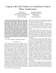
RAM, this is a positive result on memory benchmark.
5.2.4 Discussion for Micro Evaluation
Now we have finished in discussing micro evaluation for ‘SUSE’, and we have
got positive results throughout this section.This is especially an important result
for sensor network since hardware resources always restrictapplications that
running on sensors. What’s more, the purpose for us to design ‘SUSE’ is to
provide support for diagnosing other algorithms, so resource efficiency becomes
a more important feature to it.Another important thing to also note is that there is
still a space to improve its performance.
We can develop a new data collecting protocol that can provide higher collecting
efficiency. We can also enhance the serial port driver in Tmote sky, to let it
receive data in a relatively faster speed.Next, in section 5.3,we discuss the result
from macro evaluation.
5.3Macro Evaluation
In this section, we describe and discuss the result of macro evaluation of
‘SUSE’. As we have mentioned in section 5.2, we firstly simulate a scenario for
testing, we use two sensors to run Dijkstra’s algorithm, and use another sensor to
work as sink. ‘SUSE’ run on all 3 sensors to provide diagnose support. And
suppose the scenario is working in such a situation: when two sensors are
working on their Dijkstra’s algorithm, suddenly one node can not receive
anything from the
-35-
-42-
other in the second cycle of running, so we decide to start ‘SUSE’ to diagnose it.
We firstly insert the algorithm into ‘SUSE’, and suppose we have fixed all
semantic bugs already, then we firstly create a Cooja mask, and then we upload
the same source code to test bed. Suppose everything runs correctly and we
gather two checkpoint files from sensors in first cycle of running. Next we can
upload these files to Cooja and create a test bed mask, after this, we generate a
standard mask. Then we run the Dijkstra’s algorithm again and download the
checkpoint files that created in the second cycle of running. We upload the
checkpoint files to Cooja again and perform diagnosis, when it finishes, we can
get a report from database for further analysis.
First of all,we have to define two use cases for this evaluation:(1)‘SUSE’ should
not modify the variables that in name of the sensor’s state, (2) these variables
should not appear in final diagnose report. The reason for this definition is
obvious: whenever ‘SUSE’ running, itshouldn’t modify any key variables in
target program; then secondly, it should distinguish between a suspect variable
and a correct variable but always changes its value, and finally display the result
in report.We can use variable watcherto finish the first job,becauseit can provide
any variable values during the simulation.We canperform thediagnosiswith
improved simulation control panelto finish the second task.And at last, we read
final report in database.We test the scenario for several times, in this case, we
have defined two variables to work as sensors’ states: ‘node2state [1]’and
‘node3state [1]’ and weuse ‘variable watcher’ to validate them.We finally find
out that ‘SUSE’ has not affected the Dijkstra’s algorithm because both nodes
change their states correctly, and the states that read from sensors’ memory is
also correct. Actually, because we designed ‘SUSE’ in a passive working
pattern, so generally speaking, it only receives and dumps data instead of modify
any. Then we check the final report in order to find more details. At last, we find
that ‘SUSE’ distinguish suspect varaibles and correct variables
correctly.Obviously,
none of ‘states variables’ appear in final report.We can also read the physical
addresses of suspect varaiblesfrom report,which is quite important when debug
on test bed.
-36-
-43-
Figure 5.6A sample report that lists all suspect varaiblesthat has been changed
illegally, although these suspect varaiables do not mean the system must affected
by bugs, but if there is one, it would be a good idea to check these suspect
variables first.
5.3.1 Discussion
In this evaluation, we have tested ‘SUSE’ in a simulated scenario to validate its
function. Obviously it has successfully provided a variant-level debugging
support for sensor network, both functionality and performance. The advantages
of ‘SUSE’ are obvious: (1) ‘SUSE’ is an open-structure tool that composed by
series elements, so it is easy to add new features to it, or use some of its
functions separately for other purpose. What’s more, ‘SUSE’ is a powerful tool
that has the capability todebug any algorithms that are running on test bed. The
operation is also simple: just insert the target process in ‘SUSE’, then follows
the same steps to get the final diagnose report. On the contrary, there are also
some disadvantages that need pay attention to: first of all, checkpoint process
affects broadcast process, although in this research we have avoided this
problem by
-37-
-44-
reset the rime stack, but this is still a problem because we do not know the exact
reason for it. Secondly, ‘SUSE’ is a passive designed tool instead an active one,
so most commonly scenario is: we have to run the programagain with the help of
‘SUSE’ after some errors have occurred, this is more or less a waste of time
when comparing to active diagnose tool.
One important thing to also mention, if there are any suspect variables listed in
final report, it does not mean that the program ‘must’ have a bug. On the
contrary, if there is any bugs occurred in a program, most hopefully we can find
valuable clues in diagnose report. So if we can combined using ‘SUSE’ with
other diagnose tools, such as semantic checking tools, we can greatly improve
the detect rate and decrease the false alarm rate at the same time.
-38-
-45-
6 Discussion
This work presents a diagnosis tool named ‘SUSE’, which provides an efficient
and variable level diagnosis that works on both simulator and test bed.
‘SUSE’consists of four modules: ‘Snapshots collector’, ‘Up/Down loader’,
‘Standard mask creator’ and ‘Evaluator’.‘Snapshot collector’creates snapshots
on sensor nodes then collect them to sink, up/down loader transfers filesbetween
simulator, computer and test bed, ‘standard mask creator’ can generate standard
mask that works as a reference in diagnosis, and finally ‘evaluator’ performs
diagnosiswiththe help of standard mask.
Generally, there are two designing methods for diagnosis tools, one passive way
and one active way. We say that a passive diagnosis tool won’t affect the
running of sensor networks, because we do not need to run it when everything
goes correct. That is the reason why a passive tool cannot locate the suspect
variables as soon as a bug occurs. An active diagnosis tool works simultaneously
with sensor networks, which can provide a real-time monitoring on the
system.One of the disadvantages is that it needs a carefulinteraction with the
host;because there are many sensitive aspects that it has to deal with, such as
hardware resource management, switch between different contexts and system
performance. ‘SUSE’ is a passive designed diagnosis tool, so if it works together
with an active diagnosis tool, it is possible to increase the detect rate and
decrease the miss rate.
‘SUSE’ is not only a diagnosis tool, but also provides us a lot of new
availabilities to sensor networks, such as file transfer between different
platforms and files collection among several nodes. Namely, ‘SUSE’ fulfills the
requirements when we upload source code from simulator to test bed by
providing an efficient variables level diagnosis method on both platforms. We
saw that ‘SUSE’ has provided a smooth transition from simulator to test bed.
Namely, we do not need to have in mind bugs that produced on test bed but
never appeared in simulator.
-39-
-46-
Biblliography
[1] Sundaram, V., Eugster, P., and Zhang, X., Addanki, Efficient Diagnostic
Tracing for Wireless Sensor Networks. SenSys '10 Proceedings of the 8th ACM
Conference on Embedded Networked Sensor Systems, Page 169-192, 2010.
[2] Lilia Paradis, Qi Han, A Survey of Fault Management in WirelessSensor
Networks, Journal of Network and Systems Management, 2007, Volume 15
Issue 2, Pages 171 – 190.
[3] Xiaoqiao Meng, Thyaga Nandagopal, Songwu Lu.Contour Maps: Monitoring
and Diagnosis in Sensor Networks. Computer Networks - COMPUT NETW ,
2006, vol. 50, no. 15.
[4] Anmol Sheth, Carl Hartung, Richard Han, A Decentralized Fault Diagnosis
System for Wireless Sensor Networks, Mobile Adhoc and Sensor Systems
Conference, IEEE, 2005
[5] Fredrik Österlind,Adam Dunkels, Thiemo Voigt, Nicolas Tsiftes, Joakim
Eriksson, Niclas Finne. Sensornet Checkpointing: Enabling Repeatability in
Testbeds and Realism in Simulations, EWSN '09 Proceedings of the 6th
European Conference on Wireless Sensor Networks, 2007.
[6] V. Krunic, E. Trumpler, and R. Han. NodeMD: Diagnosing node-level faults
in remote wireless sensor systems. MobiSys '07 Proceedings of the 5th
international conference on Mobile systems, applications and services, 2007.
[7] Luca Mottola, Thiemo Voigt, and Fredrik Österlind: enabling efficient static
verification of sensor network software. SESENA '10 Proceedings of the 2010
ICSE Workshop on Software Engineering for Sensor Network Applications,
2010.
-40-
-47-
[8] Santi Kumari Behera, Prabira Kumar Sethy, Dr. Pabitra Mohan Khilar. Fault
Diagnosis in Wireless Sensor Network using Timed Automata, International
Journal of Computer Applications, 2011, Volume 29– No.7.
[9] Xin Miao, Kebin Liu, Yuan He, Yunhao Liu, Dimitris Papadias. Agnostic
Diagnosis: Discovering Silent Failures in Wireless Sensor Networks.
INFOCOM, 2011 Proceedings IEEE, 2011.
[10] R. Costa, S. Sargento, R. Aguiar, Instituto de Telecomunicac¸oes,
Aveiro,and W.Zhang, Development of a Hybrid Simulation and Emulation
Testbed For VANETs, Revista do DETUA, 2009,Volume. 4, No. 10.
-41-
-48-
Appendix A
Quick start
A.1Usage for ‘Snapshots Collector’
1.
Unpack Diagnose.tar.gz somewhere in your hard drive.
2.
Copy the checkpoint.c and checkpoint file into /Contiki -2.5/apps/shell/, and
overwrite the original files.
3.
Copy all files in Contiki /tools/Cooja/…./plugins/ to the same directory.
4.
Copy the 'recv_Cooja.c' and 'send_Cooja.c' into some folders then compile
them.
5.
Copy the 'recv_testbed.c' and 'send_testbed.c' into some folders then
compile them.
6.
Copy the 'collectdata.c' into /Contiki /examples/rime.
7.
Copy the 'MAKEFILE' into /Contiki /examples/rime.
8.
Enter /Contiki /tools/Cooja, and use 'ant run' to start Cooja.
9.
Use 'ant clean' can delete cache from Cooja.
10. Start a new simulation in Cooja
11. Create three new sky motes from the file 'collectdata.c', and place them
relatively close so they can hear from each other.
12. Start to run.
13. There are 30 seconds for transferring data to computer in each round of
running.
A.2 Usage for ‘Up/Downloader’
A.2.1 Transfer from Coojato Computer
-42-
-49-
1.
Wait until data collection process finishes, Coojadisplays a hint message for
starting the file transfer.
2.
Single click on the sink node, and select 'socket server'
3.
Use recv_Cooja.c to build a socket connection with Cooja.
4.
Then write click on the sink node then select 'click the button'.
5.
File transfer start and then the checkpoint files are transfer onto the hard
disk.
6.
Repeatedly to receive the other checkpoint file.
A.2.2 Transfer from Computer to Cooja
1. Start Coojathen create a new simulation.
2. Create a node with '/rime/collectdata.c'.
3. Start a socket server from the node.
4. Right click on the node and select 'click the button'.
5. From another terminal window, run the ‘send_Cooja.c’ with ‘./sendCooja’
127.0.0.1 60001 Snapshot_xx-xx-xx.
6. The node inside Coojareceives the checkpoint file.
7. Repeatedly, we can receive other checkpoint files.
8. Right click on the node and select 'click the button'.
9. Close the socket connection, and open shell terminal inside Cooja.
10. Roll back from any checkpoint.
11. Coojadisplays hint message after each transmission.
A.2.3 Transfer from Testbed to Computer
1. Wire the sink node with an USB port from computer.
2. There are 30 seconds between each two running for file transfer to
computer.
3. Start the sensors.
4. Use serial-dump to inspect the running status of sink node.
-43-
-50-
5. When collecting stops, use recv_testbed.c to build a serial connection with
sink node.
6. Push the button on sink node.
7. Data transfers from sink node to computer.
8. Repeatedly to receive other checkpoint files.
A.2.4Transfer from Computer to TestBed
1. Wire a sensor with an USB port to a computer.
2. Push the button on this sensor, it displays hint message for starting the
transmission.
3. Use send_testbed.c to send a checkpoint file to this sensor: ./sendtestbed b115200 /dev/ttyUSB0 Snapshot_xx-xx-xx
4. Repeatedly to receive other checkpoint files.
5. Now login to the shell of the sensor through a serial-dump.
6. Rollback from any checkpoint files.
A.3Usage for ‘Standard Mask Creator’
1.
Start a new simulation in Cooja.
2.
Create 3 nodes with the same code base that are going to debug with.
3.
Click on ‘C->DB’ repeatly.
4.
Click on ‘C-Mask’ to generate Coojamask.
5.
Burn the code base to test bed.
6.
Start the test bed to run.
7.
Collect checkpoint from test bed to computer follows the steps in A.2.
8.
For example, if the algorithm is running on two working nodes, and if the
program is running within a loop, then sink node collects 2 snapshots from
them in each round.
9.
Upload the checkpoint files downloaded from test bed to Cooja.
10. Rollback one checkpoint file in node 1.
-44-
-51-
11. Click ‘T->DB’.
12. Repeatedly, untill all checkpoint files imported into database.
13. Click ‘T->Mask’ to create test bed mask.
14. Click ‘Create Final mask’ to create the standard mask.
A.4Usage for ‘Evaluator’
1.
Run the code on test bedthat is going to debug with.
2.
Download checkpoint files from test bed to computer.
3.
Upload checkpoint files to Cooja(which nodes run the same code base).
4.
Click ‘Dic’ to create the variables dictionary.
5.
Rollback one checkpoint file in node 1.
6.
Click ‘D->DB’.
7.
Repeatedly, import all data checkpoint files into database.
8.
Click ‘D-Mask’ to create mask for the source code that are going to debug
with.
9.
Click ‘Diagnose’ to generate the final report.
10.
Open a database query tool to check the result.
Note: A.4 is available only after generating standard mask from same code
base that are going to debug with.
-45-
-52-
Appendix B
User manual
B.1 Basic Usage of Cooja
1.
Open a terminal in Linux then find the Cooja’s folder by: cd Contiki
/tools/Cooja
2.
Use command ‘ant run’ to start Cooja.
3.
Use file->new simulation to start a new simulation.
4.
Use Mote-types-> Sky mote to select mote type.
5.
Select the sensor code that going to run on the motes.
6.
Support for select different code base for different nodes.
7.
Press start in the control panel to start the simulations.
8.
Plugins can be added/ removed by ’motes’ menu.
9.
Left click on mote can find other useful options.
B.2 Node_id Burning
New sensor nodes should be burned with a unique node_id as their only
identification. Contiki provide a program named burn-nodeid.c, which located in
Contiki /platform/sky/apps.
B.3 Upload Code
Use ‘make codename.upload TARGET=sky’ to upload sensor code onto
testbeds, for example: ‘make collect.upload TARGET=sky’.
Code can upload simultaneously to all sensor nodes if they are connected with a
hub.
-46-
-53-
Appendix C
Sensor Code
SourceCode.zip
-47-54-