Download MicroCal ITC-200 User Manual - Center for Macromolecular

MicroCal iTC200 system
User Manual
MAN0560-01-EN-00 August 2014
Copyright © 2014 Malvern Instruments Ltd.
Malvern Instruments pursues a policy of continual improvement due to technical
development. We therefore reserve the right to deviate from information, descriptions,
and specifications in this publication without notice. Malvern Instruments shall not be
liable for errors contained herein or for incidental or consequential damages in
connection with the furnishing, performance or use of this material. No reproduction
or transmission of any part of this publication is allowed without the express written
permission of Malvern Instruments Ltd.
Head office:
Malvern Instruments Ltd.
Grovewood Road,
Malvern,
Worcestershire, WR14 1XZ
United Kingdom.
Tel +44 1684 892456
Fax +44 1684 892789
MicroCal, Malvern and the 'hills' logo are registered trademarks in the UK and/or other
countries, and are owned by Malvern Instruments Ltd
Windows is a registered trademark of Microsoft Corporation
.
Table of Contents
Table of Contents
1
Introduction ..........................................................................................................
1.1
1.2
1.3
1.4
2
3
4
5
7
Important user information .............................................................................................................
About this manual ................................................................................................................................
Regulatory information ......................................................................................................................
Associated documentation ..............................................................................................................
8
10
11
12
MicroCal iTC200 .....................................................................................................
13
2.1
2.2
Overview of an isothermal titration calorimeter ....................................................................
Description of MicroCal iTC200 ........................................................................................................
14
18
Installation ............................................................................................................
21
3.1
Setting up MicroCal iTC200 before a run .....................................................................................
3.1.1
Fluid connections ...............................................................................................................................
3.1.2
Bottle preparation ..............................................................................................................................
3.1.3
Hardware connections ....................................................................................................................
3.2
Installing MicroCal iTC200 software ...............................................................................................
3.2.1
Updating the software .....................................................................................................................
3.2.2
Complete installation of the software .......................................................................................
3.3
Settings for Windows 7 ......................................................................................................................
3.3.1
Modify the Origin 7 configuration for Windows 7 ................................................................
3.3.2
Modify the MicroCal iTC200 software configuration for Windows 7 .............................
3.3.3
Modify the user account control settings for Windows 7 .................................................
22
23
27
30
35
36
41
49
50
52
54
Control software ..................................................................................................
56
4.1
Overview ...................................................................................................................................................
4.2
MicroCal iTC200 software ...................................................................................................................
4.2.1
Starting MicroCal iTC200 software ...............................................................................................
4.2.2
MicroCal iTC200 software interface overview .........................................................................
4.2.3
MicroCal iTC200 software control buttons ................................................................................
4.2.4
Experimental Design tab ..............................................................................................................
4.2.5
Advanced Experimental Design tab .......................................................................................
4.2.6
Instrument Controls tab ...............................................................................................................
4.2.7
Real Time Plot tab .............................................................................................................................
4.2.8
Setup tab ...............................................................................................................................................
4.2.9
MicroCal iTC200 software menus .................................................................................................
4.3
Origin for real-time data display ...................................................................................................
57
58
59
60
61
62
65
72
77
78
80
84
Performing a run ..................................................................................................
87
5.1
Preparing the samples .......................................................................................................................
5.1.1
The importance of sample preparation ...................................................................................
5.1.2
Preparing small molecule solutions ...........................................................................................
5.1.3
Preparing macromolecule solutions ..........................................................................................
5.1.4
Calculating cell concentrations ....................................................................................................
5.1.5
Syringe concentration and number of injections .................................................................
88
89
90
91
93
97
MicroCal
User Manual
MAN0560
MicroCal iTC200
iTC200 System
User Manual
29017607
AA
3
Table of Contents
6
4
5.1.6
Experimental temperature and control heat determination ...........................................
5.1.7
Additional notes ..................................................................................................................................
5.2
Creating a method ...............................................................................................................................
5.3
Cleaning the cell and syringe before performing an experiment ..................................
5.3.1
Cell and syringe wash ......................................................................................................................
5.3.2
Cell buffer rinse (short) .....................................................................................................................
5.3.3
Cell water rinse (long) .......................................................................................................................
5.3.4
Detergent soak and rinse (long) ...................................................................................................
5.3.5
Syringe wash (short) .........................................................................................................................
5.3.6
Syringe wash (long) ...........................................................................................................................
5.3.7
Dry syringe ............................................................................................................................................
5.4
Loading the samples and performing the experiment .......................................................
5.4.1
Loading the titration syringe .........................................................................................................
5.4.2
Loading the cell ...................................................................................................................................
5.4.3
Performing an experiment .............................................................................................................
5.4.4
Procedures after an experiment ..................................................................................................
98
99
100
103
104
105
106
107
108
109
110
111
112
114
115
116
Data analysis using Origin .................................................................................
118
6.1
6.1.1
6.1.2
6.1.3
6.2
6.3
6.3.1
6.3.2
6.3.3
6.4
6.4.1
6.4.2
6.4.3
6.4.4
6.5
6.5.1
6.5.2
6.5.3
6.6
6.6.1
6.6.2
6.6.3
6.6.4
6.6.5
6.6.6
6.6.7
6.6.8
6.6.9
119
120
121
131
136
143
144
150
152
161
162
166
168
171
172
173
177
179
181
183
195
201
206
209
212
213
222
224
Basic ITC data analysis and fitting ................................................................................................
Starting Origin .....................................................................................................................................
Routine ITC data analysis ...............................................................................................................
Creating a final figure for publication .......................................................................................
Adjusting baseline and integration range .................................................................................
Analyzing multiple runs and subtracting reference .............................................................
Opening multiple data files ............................................................................................................
Adjusting the molar ratio ................................................................................................................
Subtracting reference data ............................................................................................................
ITC data handling ..................................................................................................................................
Reading worksheet values from plotted data .......................................................................
Copy and paste worksheet data .................................................................................................
Exporting worksheet data ..............................................................................................................
Importing worksheet data .............................................................................................................
Modifying templates ............................................................................................................................
Modifying the DeltaH template ...................................................................................................
Modifying the RawITC template ..................................................................................................
Units notation in Origin ....................................................................................................................
Advanced curve fitting .......................................................................................................................
Nonlinear curve fitting .....................................................................................................................
Fitting with the two sets of sites model ..................................................................................
Reverse titrations ...............................................................................................................................
The Sequential Binding Sites model ........................................................................................
Binding of multiple ligands to transition metal ions ...........................................................
Enzyme/substrate/inhibitor assay ..............................................................................................
Method 1A: Enzyme assay- substrate only .............................................................................
Method 1B: Enzyme assay- substrate plus inhibitor ...........................................................
Method 2A: Enzyme assay- substrate only .............................................................................
MicroCal iTC200 User Manual 29017607 AA
Table of Contents
7
8
9
A
6.6.10 Method 2B: Enzyme assay- substrate plus inhibitor ...........................................................
6.6.11 Dimer dissociation model ...............................................................................................................
6.6.12 Competitive ligand binding ............................................................................................................
6.6.13 Simulating curves ...............................................................................................................................
6.6.14 Single injection method (SIM) ........................................................................................................
6.7
Other useful details ..............................................................................................................................
227
229
232
235
238
248
Maintenance .........................................................................................................
253
7.1
7.2
7.3
7.4
7.5
Cleaning the cell ....................................................................................................................................
Refilling the reference cell ................................................................................................................
Washing module ...................................................................................................................................
Replacing the syringe plunger tip .................................................................................................
Replacing and cleaning the titration syringe ...........................................................................
254
255
256
261
268
Troubleshooting ...................................................................................................
278
8.1
8.2
8.3
8.4
8.5
8.6
8.7
8.8
8.9
8.10
Peaks too large ......................................................................................................................................
Broad peaks ............................................................................................................................................
Downward stepping baseline .........................................................................................................
Upward stepping baseline ................................................................................................................
Reversed/oscillating peaks ..............................................................................................................
Baseline spikes .......................................................................................................................................
Low baseline ...........................................................................................................................................
Abnormal peaks ....................................................................................................................................
Unexpected thermodynamic results ...........................................................................................
Washing Module ...................................................................................................................................
279
281
283
284
285
286
288
290
292
294
Reference information ........................................................................................
296
9.1
9.2
9.3
9.4
9.5
How to get help .....................................................................................................................................
Networking ..............................................................................................................................................
MicroCal iTC200 ITC methods ...........................................................................................................
MicroCal iTC200 specifications .........................................................................................................
Reagents ...................................................................................................................................................
297
299
306
307
309
Equations used for fitting ITC data ...................................................................
310
Index .......................................................................................................................
324
MicroCal
User Manual
MAN0560
MicroCal iTC200
iTC200 System
User Manual
29017607
AA
5
6
MicroCal iTC200 System User Manual MAN0560
1 Introduction
1
Introduction
Introduction
This chapter contains important user information, description of safety notices, reference
for regulatory information, intended use of the MicroCal iTC200 system, a lists of associated documentation.
In this chapter
This chapter contains the following sections:
Section
1.1 Important user information
See page
8
1.2 About this manual
10
1.3 Regulatory information
11
1.4 Associated documentation
12
MicroCal
User Manual
MAN0560
MicroCal iTC200
iTC200 System
User Manual
29017607
AA
7
1 Introduction
1.1 Important user information
1.1
Important user information
Read this before operating
MicroCal iTC200
All users must read the entire Operating Instructions before installing, operating, or
maintaining the instrument. Always keep the Operating Instructions at hand when operating MicroCal iTC200.
Do not operate MicroCal iTC200 in any other way than described in the user documentation. If you do, you may be exposed to hazards that can lead to personal injury, and you
may cause damage to the equipment.
Intended use
MicroCal iTC200 is an isothermal titration calorimeter designed for biomolecular interaction
studies in research applications.
MicroCal iTC200 is intended for research use only, and shall not be used in any clinical
procedures, or for diagnostic purposes.
Prerequisites
In order to operate the system in the way it is intended, the following prerequisites must
be fulfilled:
8
•
You should have a general understanding of the use of a personal computer running
Microsoft™ Windows™ in the version provided with your product.
•
You should understand the concepts of isothermal titration calorimetry.
•
You must read and understand the Safety Instructions as outlined in
MicroCal iTC200 Operating Instructions.
•
The instrument and software must be installed, configured and calibrated as outlined
in MicroCal iTC200 Operating Instructions by Malvern Instruments personnel.
MicroCal
iTC200
System
User
Manual
MAN0560
MicroCal
iTC200
User
Manual
29017607
AA
1 Introduction
1.1 Important user information
Safety notices
This user documentation contains WARNINGS, CAUTIONS and NOTICES concerning the
safe use of the product with meanings as defined below.
Warnings
WARNING
WARNING indicates a hazardous situation which, if not avoided,
could result in death or serious injury. It is important not to proceed
until all stated conditions are met and clearly understood.
Cautions
CAUTION
CAUTION indicates a hazardous situation which, if not avoided,
could result in minor or moderate injury. It is important not to proceed until all stated conditions are met and clearly understood.
Notices
NOTICE
NOTICE indicates instructions that must be followed to avoid
damage to the product or other equipment.
Notes and tips
Note:
A Note is used to indicate information that is important for trouble-free and
optimal use of the product.
Tip:
A tip contains useful information that can improve or optimize your procedures.
MicroCal
User Manual
MAN0560
MicroCal iTC200
iTC200 System
User Manual
29017607
AA
9
1 Introduction
1.2 About this manual
1.2
About this manual
Purpose of the user manual
This user manual provides instructions needed to run MicroCal iTC200 and to analyze
isothermal titration calorimetry (ITC) data. This user manual is a complement to
MicroCal iTC200 Operating Instructions.
Typographical conventions
Software items are identified in the text by bold italic text. A colon separates menu levels,
thus File:Open refers to the Open command in the File menu.
Hardware items are identified in the text by bold text (e.g., Power switch).
Text entries that MicroCal iTC200 software generates or that the user must type are represented by a monotype typeface (e.g., C:\Origin70\Samples).
10
MicroCal
iTC200
System
User
Manual
MAN0560
MicroCal
iTC200
User
Manual
29017607
AA
1 Introduction
1.3 Regulatory information
1.3
Regulatory information
For regulatory information regarding MicroCal iTC200, refer to MicroCal iTC200 Operating
Instructions.
MicroCal
User Manual
MAN0560
MicroCal iTC200
iTC200 System
User Manual
29017607
AA
11
1 Introduction
1.4 Associated documentation
1.4
Associated documentation
Introduction
This section lists the user documentation that is delivered with MicroCal iTC200 and related
literature that can be downloaded or ordered from Malvern Instruments.
User documentation
The user documentation for MicroCal iTC200 consists of:
•
MicroCal iTC200 Operating Instructions
•
MicroCal iTC200 User Manual (this manual)
Related literature
Additional downloadable material can be found at: www.malvern.com/microcal
12
MicroCal
iTC200
System
User
Manual
MAN0560
MicroCal
iTC200
User
Manual
29017607
AA
2 MicroCal iTC200
2
MicroCal iTC200
Introduction
This section gives an overview of ITC and the MicroCal iTC200 system.
In this chapter
This chapter contains the following sections:
Section
See page
2.1 Overview of an isothermal titration calorimeter
14
2.2 Description of MicroCal iTC200
18
MicroCal
User Manual
MAN0560
MicroCal iTC200
iTC200 System
User Manual
29017607
AA
13
2 MicroCal iTC200
2.1 Overview of an isothermal titration calorimeter
2.1
Overview of an isothermal titration calorimeter
Introduction
Isothermal Titration Calorimeters (ITC) measure the heat change that occurs when two
substances interact. Heat is liberated or absorbed as a result of the redistribution of
noncovalent bonds, for example, when the interacting molecules go from the free to the
bound state.
An ITC mixes the binding partners and monitors these heat changes by measuring the
power required to maintain zero temperature difference between the reference and
sample cells (see Main components of an ITC, on page 15).
The reference cell usually contains water, which has the same heat capacity as most of
the sample buffers. The sample cell contains:
•
one of the binding partners (often, but not necessarily a macromolecule), and
•
a stirring syringe, which holds the other binding partner (often, but not necessarily
a ligand).
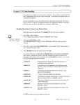
Procedure
Typically, the ligand is injected into the sample cell, in 2 to 3 μl aliquots, until its concentration is two- to three-fold greater than that of the sample cell material. Each injection
of the ligand results in a heat signature that is first integrated with respect to time and
then normalized for concentration. This titration curve is fitted to a binding model to
extract the affinity (KD), stoichiometry (n) and the enthalpy of interaction (ΔH).
An example experimental curve is depicted below.
14
MicroCal
iTC200
System
User
Manual
MAN0560
MicroCal
iTC200
User
Manual
29017607
AA
2 MicroCal iTC200
2.1 Overview of an isothermal titration calorimeter
Notice that the first injection results in a larger deflection from the baseline, denoting a
larger heat and nearly 100% binding. At the conclusion of the experiment, very little of
the injected substance binds, resulting in little or no deflection from baseline (heat).
Also, notice that the value on the y-axis decreases upon binding. In other words, this is
the power needed to keep the sample cell at the same temperature as the reference
cell.
Heat is given off during the reaction, therefore less power is required to compensate the
temperature differences. This is characteristic of an exothermic reaction. In contrast, an
endothermic reaction results in spikes rising from the baseline and hence, more power
is required to compensate the temperature differences.
Main components of an ITC
The main components of an ITC system are illustrated below:
1
2
3
4
5
6
7
8
9
10
Part
Description
1
Sensor
2
Lead screw
MicroCal
User Manual
MAN0560
MicroCal iTC200
iTC200 System
User Manual
29017607
AA
15
2 MicroCal iTC200
2.1 Overview of an isothermal titration calorimeter
Part
Description
3
Injector
4
Plunger
5
Stirring syringe
6
Syringe
7
Outer shield
8
Inner shield
9
Sample cell
10
Reference cell
Raw data
The temperature difference between the sample cell and the reference cell is converted
to power and directly read out as raw data. An example of this is depicted below. Each
spike, followed by a return to the baseline, is an injection.
16
MicroCal
iTC200
System
User
Manual
MAN0560
MicroCal
iTC200
User
Manual
29017607
AA
2 MicroCal iTC200
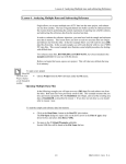
2.1 Overview of an isothermal titration calorimeter
Injection heat
The individual injection heats are calculated by integrating the raw data (power) from
each injection over time. The figure below depicts each individual injection heat,
normalized by the amount of titrant injected, as a function of the molar ratio of titrant/cell
material in the sample cell. The fitted curve of a 1:1 binding model is overlaid in red. A
general illustration of how the thermodynamic parameters n, KD, and ΔH are related to
the titration curve is also overlaid.
In the case of this simple 1:1 binding experiment, the enthalpy is directly measured/fitted
as the heat of 100% binding. The stoichiometry is intuitively denoted by the midpoint of
the titration, between 100% binding and 0% binding. The steepness of the rise to
saturation is related to binding affinity. For any given system, the steepness of this region
is also directly related to the sample concentration.
Data analysis will be explained in more detail in Chapter 6 Data analysis using Origin, on
page 118.
MicroCal
User Manual
MAN0560
MicroCal iTC200
iTC200 System
User Manual
29017607
AA
17
2 MicroCal iTC200
2.2 Description of MicroCal iTC200
2.2
Description of MicroCal iTC200
Introduction
MicroCal iTC200 provides detailed insight into binding energetics.
The system has a 200 μl sample cell and provides direct measurement of the heat
absorbed or evolved as a result of mixing precise amounts of reactants. The sample and
reference cells are made from Hastelloy™, a highly inert material.
Data analysis is performed using Origin™ software, wherein the user obtains the stoichiometry (n), dissociation constant (KD), and enthalpy (ΔH) of the interaction. The Origin
software can also be used to fit more complicated models.
18
MicroCal
iTC200
System
User
Manual
MAN0560
MicroCal
iTC200
User
Manual
29017607
AA
2 MicroCal iTC200
2.2 Description of MicroCal iTC200
Primary components of
MicroCal iTC200
The primary components of MicroCal iTC200 are illustrated below.
1
2
3 4
5
6
7
8
9
Part
Description
1
Reagent bottles
2
Loading syringe
3
Cleaning module
4
Washing module
5
Fill port adapter (FPA)
6
Pipette
7
Wash/load station
8
Titrant loading station
9
Calorimeter
MicroCal
User Manual
MAN0560
MicroCal iTC200
iTC200 System
User Manual
29017607
AA
19
2 MicroCal iTC200
2.2 Description of MicroCal iTC200
Connections at the rear of the
MicroCal iTC200 cell unit
The illustration below shows the rear of the MicroCal iTC200 cell unit.
1
2
3
4
6
20
Part
Function
1
Fan
2
Main power switch
3
Power fuses
4
IEC 320 inlet power receptacle
5
USB connectors
6
µP activity indicator
5
MicroCal
iTC200
System
User
Manual
MAN0560
MicroCal
iTC200
User
Manual
29017607
AA
3 Installation
3
Installation
Introduction
This chapter describes how to set up MicroCal iTC200 before a run, the installation of
MicroCal iTC200 software and settings for Windows 7.
Information about Networking, see Section 9.2 Networking, on page 299.
In this chapter
This chapter contains the following sections:
Section
See page
3.1 Setting up MicroCal iTC200 before a run
22
3.2 Installing MicroCal iTC200 software
35
3.3 Settings for Windows 7
49
MicroCal
User Manual
MAN0560
MicroCal iTC200
iTC200 System
User Manual
29017607
AA
21
3 Installation
3.1 Setting up MicroCal iTC200 before a run
3.1
Setting up MicroCal iTC200 before a run
Introduction
This chapter describes the preparations and how to set up MicroCal iTC200 before a run.
In this chapter
This chapter contains the following sections:
Section
22
See page
3.1.1 Fluid connections
23
3.1.2 Bottle preparation
27
3.1.3 Hardware connections
30
MicroCal
iTC200
System
User
Manual
MAN0560
MicroCal
iTC200
User
Manual
29017607
AA
3 Installation
3.1 Setting up MicroCal iTC200 before a run
3.1.1 Fluid connections
3.1.1
Fluid connections
Fluid connections on the
MicroCal iTC200 instrument
Fluid connections for the MicroCal iTC200 system are provided. To mount the connections,
follow the steps described below:
Step
Action
1
Connect the line from the top of the
cell cleaning module to port C3 on
the left side of the washing module.
2
Connect the line that originates at the
side of the cell cleaning module to
port C4 on the left side of the washing
module.
3
Connect the waste line to port C5 on the left side of the washing module.
4
Connect Syringe Needle Cleaning Tube (ASY020512) from the port on the
Wash Dry Station on the right side of cell unit (left image below) to port C2
on the right side of the washing module (right image below).
MicroCal
User Manual
MAN0560
MicroCal iTC200
iTC200 System
User Manual
29017607
AA
23
3 Installation
3.1 Setting up MicroCal iTC200 before a run
3.1.1 Fluid connections
24
Step
Action
5
Connect the red ferrule (see arrow) of the fill port adapter (FPA) (ASY020506)
to port C1 on the right side of the instrument.
6
Screw the FPA into the top right block in the rear of the washing module,
and turn it down until it is flush with the top of the housing.
MicroCal
iTC200
System
User
Manual
MAN0560
MicroCal
iTC200
User
Manual
29017607
AA
3 Installation
3.1 Setting up MicroCal iTC200 before a run
3.1.1 Fluid connections
Connect tubing from the bottles
To connect the tubing from the bottles to the bottle adapter, follow the steps described
below:
Step
Action
1
•
Connect the blue bottle to the water inlet port
•
Connect the red bottle to the methanol inlet port
•
Connect the white bottle to the buffer inlet port
Note:
Do not over-tighten.
2
Remove the securing nut from the top of the waste bottle and slide
the open end of the waste tubing through it.
3
Slide the ferrule over the tubing with the cone end facing towards
the securing nut, see the illustration below.
Note:
The opposite end of the waste tube should be installed in the C5 port
on the washing module. See the step-action table in Fluid connections
on the MicroCal iTC200 instrument, on page 23 above.
MicroCal
User Manual
MAN0560
MicroCal iTC200
iTC200 System
User Manual
29017607
AA
25
3 Installation
3.1 Setting up MicroCal iTC200 before a run
3.1.1 Fluid connections
26
Step
Action
4
Insert the waste line (connected to the C5 port on the washing
module) into the grey (waste) bottle and tighten the securing nut
until it is finger tight.
5
Bundle the three fluid lines from the adapter and position them so
they will not interfere with your experiments.
MicroCal
iTC200
System
User
Manual
MAN0560
MicroCal
iTC200
User
Manual
29017607
AA
3 Installation
3.1 Setting up MicroCal iTC200 before a run
3.1.2 Bottle preparation
3.1.2
Bottle preparation
Before running an experiment, you may need to perform one or all of the following tasks:
•
Bottle preparation
•
Filling bottles
•
Priming tubing
•
Emptying the waste bottle
Bottle preparation
Use this procedure to prepare the bottles before using the washing module. There are
three bottles that you must maintain:
•
Water: bottle with blue top
•
Methanol: bottle with red top
•
Buffer: bottle with white top
Filling bottles
Although the bottles do not have to be full before you begin a procedure, you should
make sure that there is sufficient volume in each bottle to perform the required procedure.
To fill the bottles, follow the steps described below:
Step
Action
1
Verify that the system is in an idle state.
MicroCal
User Manual
MAN0560
MicroCal iTC200
iTC200 System
User Manual
29017607
AA
27
3 Installation
3.1 Setting up MicroCal iTC200 before a run
3.1.2 Bottle preparation
Step
Action
2
Unscrew the plastic cap of the bottle by turning it
counter-clockwise.
3
Fill bottle using standard lab procedures.
4
Tighten the cap by turning clockwise until snug.
Priming tubing
Use this procedure to prime the tubing from the bottles to the washing module to make
sure that the full volume is delivered. This procedure is required only if the tubes leading
from the bottles to the washing module have been drained of fluid and contain air.
Step
Action
1
Make sure all bottles have sufficient volume and all fluid lines are connected.
2
Click Cell Buffer Rinse (Short) on the Instrument Controls tab.
3
Click Syringe Wash (Long) on the Instrument Controls tab.
After tubings have been primed (visibly clear of air), the system uses the majority of the
remaining procedure time to dry the syringe. This occurs with approximately eight minutes
remaining in the procedure. You can let the procedure finish or click Cancel at this time.
Emptying the waste bottle
Use this procedure to empty the waste bottle.
28
Step
Action
1
Verify that the system is in an idle state.
MicroCal
iTC200
System
User
Manual
MAN0560
MicroCal
iTC200
User
Manual
29017607
AA
3 Installation
3.1 Setting up MicroCal iTC200 before a run
3.1.2 Bottle preparation
Step
Action
2
Unscrew the grey cap of waste bottle by turning the lid counter-clockwise.
3
Empty the waste according to your laboratory waste handling procedures.
4
Reattach the cap by turning it clockwise until it is snug.
MicroCal
User Manual
MAN0560
MicroCal iTC200
iTC200 System
User Manual
29017607
AA
29
3 Installation
3.1 Setting up MicroCal iTC200 before a run
3.1.3 Hardware connections
3.1.3
Hardware connections
Introduction
The washing module, the MicroCal iTC200 controller PC and the MicroCal iTC200 cell unit
are connected through a standard USB 4-port hub.
The following hardware is required to connect the three parts of MicroCal iTC200:
•
One USB 2.0 4-port hub
•
One type A-B (mini) USB connector
•
Two type A-B (standard) USB connectors
Part
Description
USB 2.0 4-port hub
USB Connector type A
USB Connector type B (mini)
USB Connector type B (standard)
30
MicroCal
iTC200
System
User
Manual
MAN0560
MicroCal
iTC200
User
Manual
29017607
AA
3 Installation
3.1 Setting up MicroCal iTC200 before a run
3.1.3 Hardware connections
Mounting the hardware
connections
To mount the hardware connections, follow the steps described below:
Step
Action
1
Identify the only cable with the USB type B (mini) cable end.
Connect the type B (mini) cable end to the USB hub.
Connect the USB type A end of that cable to the labeled Controller PC USB
port.
2
Connect the USB type A ends of two USB cables to the hub.
3
Connect the USB type B ends to the USB 1 and USB 2 connectors on the
rear of the MicroCal iTC200 cell unit. For illustration, see Connections at the
rear of the MicroCal iTC200 cell unit, on page 20.
4
Place the washing module on top of the MicroCal iTC200 cell unit.
When properly positioned, the feet on the washing module will fit into the
depressions on the top of the cell unit to keep it from sliding off.
5
Connect the USB type A end from the washing module to the hub.
MicroCal
User Manual
MAN0560
MicroCal iTC200
iTC200 System
User Manual
29017607
AA
31
3 Installation
3.1 Setting up MicroCal iTC200 before a run
3.1.3 Hardware connections
Step
Action
6
Connect the green grounding strap wire between the washing module and
the MicroCal iTC200 cell unit.
The illustration below shows the rear of the washing module and the MicroCal
iTC200 cell unit.
32
MicroCal
iTC200
System
User
Manual
MAN0560
MicroCal
iTC200
User
Manual
29017607
AA
3 Installation
3.1 Setting up MicroCal iTC200 before a run
3.1.3 Hardware connections
Electrical connections for the cell
unit
To connect the cell unit to the electrical supply, follow the steps described below:
Step
Action
1
Connect the power cord to the IEC 320 inlet power receptacle on the back
of the cell unit. (For illustration, see Connections at the rear of the
MicroCal iTC200 cell unit, on page 20.)
2
Connect the power plug to a main power supply receptacle with a 3-wire
protective Earth ground and a Ground Fault Circuit Interrupter (GFCI).
WARNING
Always plug the instrument into a Ground Fault Circuit Interrupter
(GFCI).
Electrical Connections for the
Washing Module
The illustration below shows the washing module power supply unit.
To connect the washing module to the electrical supply, follow the steps described below:
Step
Action
1
Connect the power cord from the power supply to the power receptacle on
the rear of the washing module.
2
Connect the power supply to a main power supply receptacle with a 3-wire
protective Earth ground and a Ground Fault Circuit Interrupter (GFCI).
MicroCal
User Manual
MAN0560
MicroCal iTC200
iTC200 System
User Manual
29017607
AA
33
3 Installation
3.1 Setting up MicroCal iTC200 before a run
3.1.3 Hardware connections
WARNING
To enhance safety always plug the instrument into a Ground Fault
Circuit Interrupter (GFCI).
34
MicroCal
iTC200
System
User
Manual
MAN0560
MicroCal
iTC200
User
Manual
29017607
AA
3 Installation
3.2 Installing MicroCal iTC200 software
3.2
Installing MicroCal iTC200 software
Introduction
If a previous version of software is installed on the controller, then follow the software
update instructions described in Section3.2.1 Updating the software, on page36 otherwise
follow the instructions for a full installation in Section 3.2.2 Complete installation of the
software, on page 41.
In this section
This section contains the following topics:
Section
See page
3.2.1 Updating the software
36
3.2.2 Complete installation of the software
41
MicroCal
User Manual
MAN0560
MicroCal iTC200
iTC200 System
User Manual
29017607
AA
35
3 Installation
3.2 Installing MicroCal iTC200 software
3.2.1 Updating the software
3.2.1
Updating the software
Note:
Installation of the control software requires administrative privileges.
Removing previous versions of
the OriginAddOn application
To remove previous versions of the OriginAddOn application, follow the steps described
below:
Step
Action
1
Navigate to Start:Control Panel.
2
Select Add/Remove Programs (Windows XP) or Programs and Features
(Windows 7).
3
Select OriginAddOn and click Remove/Uninstall.
Updating the control software
The control software CD contains the following applications:
•
MicroCal iTC200 software
•
USB driver for injector
•
USB driver for data aquisition
•
InitDT service
•
.Net runtime
To update the control software, follow the steps described below:
36
MicroCal
iTC200
System
User
Manual
MAN0560
MicroCal
iTC200
User
Manual
29017607
AA
3 Installation
3.2 Installing MicroCal iTC200 software
3.2.1 Updating the software
Step
Action
1
Insert the CD into the CD-ROM drive of the PC.
The CD runs automatically and the MicroCal Setup window appears.
Note:
If the CD does not start automatically, run iTC200Setup.exe from the CD.
2
Click on the iTC200 Software Update button for the installation to start automatically.
3
Follow the on-screen instructions and click Finish when the installation is
complete.
4
Select the option to restart the computer. Shortcut icons are created on the
desktop automatically.
5
Exit the main menu, remove the CD and keep it in a safe place after the applications has been installed as described.
MicroCal
User Manual
MAN0560
MicroCal iTC200
iTC200 System
User Manual
29017607
AA
37
3 Installation
3.2 Installing MicroCal iTC200 software
3.2.1 Updating the software
Updating analysis software
The MicroCal iTC200 Analysis Software and License CD (formerly called the Origin analysis
software installation CD) contains the following applications:
•
Origin 7.0 (for scientific graphing and analysis)
•
Origin Service Pack 4
•
MicroCal AddOn for Origin 7.0 (for data analysis specific to MicroCal iTC200 applications)
To update the Origin Data Analysis Add-On follow the steps described below:
Step
Action
1
Insert the CD into the CD-ROM drive of the PC.
The CD runs automatically and the MicroCal's Setup window appears.
2
Install only the Origin Data Analysis Add-On.
3
Click the Install Origin Data Analysis Add-On button.
Note:
Make sure that the Yes, I wish to install an Add-On disk now option is
checked in the pop-up window.
4
38
Click Next.
MicroCal
iTC200
System
User
Manual
MAN0560
MicroCal
iTC200
User
Manual
29017607
AA
3 Installation
3.2 Installing MicroCal iTC200 software
3.2.1 Updating the software
Step
Action
5
The destination directory path will be automatically loaded.
Click Next.
6
The software prompts for the add-on disc.
Note:
All add-on software is located on the analysis software installation disc and
there is no need to insert any additional disc.
7
Specify the path for the disc by clicking the Browse button.
8
Select the CD drive that has the analysis software installation disc in it.
Tip:
This is usually the D:\ drive.
MicroCal
User Manual
MAN0560
MicroCal iTC200
iTC200 System
User Manual
29017607
AA
39
3 Installation
3.2 Installing MicroCal iTC200 software
3.2.1 Updating the software
Step
Action
9
Double-click on the custom folder, addon_disk_7.20 and click OK.
The path is now specified.
10
Click OK to continue.
It may take a few minutes for the files to be installed.
11
Once the files have been installed, follow the on-screen instructions.
12
Click Finish to complete the installation.
After installing all the applications, exit the main menu, remove the CD and keep it in a
safe place.
Restart the PC to complete the setup.
40
MicroCal
iTC200
System
User
Manual
MAN0560
MicroCal
iTC200
User
Manual
29017607
AA
3 Installation
3.2 Installing MicroCal iTC200 software
3.2.2 Complete installation of the software
3.2.2
Complete installation of the software
Note:
Installation of software requires administrative privileges.
Installing the control software
The control software CD contains the following applications:
•
MicroCal iTC200 software
•
USB driver for injector
•
USB driver for data acquisition
•
InitDT service
•
.Net runtime
To install the control software, follow the steps described below:
Installing the MicroCal iTC200 software
To install the MicroCal iTC200 software, follow the steps described below:
Step
Action
1
Insert the CD into the CD-ROM drive of the PC.
The CD runs automatically and the MicroCal Setup window appears.
Note:
If the CD does not start automatically, run iTC200Setup.exe from the CD.
2
Click on the iTC200 Software Full Install button for the installation to start
automatically.
3
Follow the on-screen instructions and click Finish when the installation is
complete.
MicroCal
User Manual
MAN0560
MicroCal iTC200
iTC200 System
User Manual
29017607
AA
41
3 Installation
3.2 Installing MicroCal iTC200 software
3.2.2 Complete installation of the software
Step
Action
4
Restart the computer.
Be sure to select the option to restart the computer. Shortcut icons are created on the desktop automatically.
Installing the driver for the injector USB
To install the USB driver for the injector, click the Injector USB Driver button in the main
menu to start the installation. A command window opens while the driver is being installed. This window closes automatically when the driver installation is complete.
Installing the driver for data acquisition USB
To install the USB driver for data acquisition, follow the steps described below:
Step
Action
1
Click the Data Acquisition USB driver button in the main menu.
2
Follow the on-screen instructions.
3
Click Finish when the installation is complete.
Installing .Net runtime
Note:
Installation of .Net runtime is necessary before installing InitDT service.
To install the .Net runtime application, follow the steps described below:
42
Step
Action
1
Click the Install .Net Runtime button.
2
Follow the on-screen instructions.
3
Click Finish to complete the setup.
MicroCal
iTC200
System
User
Manual
MAN0560
MicroCal
iTC200
User
Manual
29017607
AA
3 Installation
3.2 Installing MicroCal iTC200 software
3.2.2 Complete installation of the software
Installing InitDT service
Note:
The InitDT service is a low level service that runs in the background of the
MicroCal iTC200 software. This service operates only in the Windows administrator mode.
To install the InitDT service, follow the steps described below:
Step
Action
1
Click the Install InitDT Service button.
2
Follow the on-screen instructions. Use the default settings.
3
Click Next to continue with the installation.
4
Click Close to exit the setup after the installation is complete.
After installing the applications, exit the main menu, remove the CD and keep it in a safe
place.
Restart the PC to complete the setup.
Installing analysis software
The MicroCal iTC200 Analysis Software and License CD (formerly called the Origin analysis
software installation CD) contains the following applications:
•
Origin 7.0 (for scientific graphing and analysis)
•
Origin Service Pack 4
MicroCal
User Manual
MAN0560
MicroCal iTC200
iTC200 System
User Manual
29017607
AA
43
3 Installation
3.2 Installing MicroCal iTC200 software
3.2.2 Complete installation of the software
•
MicroCal AddOn for Origin 7.0 (for data analysis specific to MicroCal iTC200 applications)
To install the analysis software follow the steps described below:
Step
Action
1
Insert the CD into the CD-ROM drive of the PC.
The CD runs automatically and the MicroCal's Setup window appears.
2
Install each application in the main menu as described later in this section.
Installing Origin 7.0
To install Origin 7.0, follow the steps described below:
44
Step
Action
1
Click the 1. Install Origin 7.0 button to start the installation.
2
Click on Origin 7.0 in the pop-up window.
MicroCal
iTC200
System
User
Manual
MAN0560
MicroCal
iTC200
User
Manual
29017607
AA
3 Installation
3.2 Installing MicroCal iTC200 software
3.2.2 Complete installation of the software
Step
Action
3
Follow the on-screen instructions to continue.
The Origin Setup window for Customer Information appears.
4
Enter the User Name and Company Name.
5
Locate the serial number on the front of the CD case or on the Origin box.
Enter this number including the dashes, in the Serial Number text box.
6
Click Next.
The Origin Setup window for Destination Directory appears.
MicroCal
User Manual
MAN0560
MicroCal iTC200
iTC200 System
User Manual
29017607
AA
45
3 Installation
3.2 Installing MicroCal iTC200 software
3.2.2 Complete installation of the software
Step
Action
7
The destination directory path will be automatically loaded.
Click Next.
8
Follow the on-screen instructions. It is recommended to use the default
settings.
9
Click Finish to complete the installation.
10
Exit the Origin 7.0 setup.
Installing Origin Service Pack 4
To install Origin Service Pack 4, follow the steps described below:
Step
Action
1
Click the 2. Install Origin Service Pack 4 button.
2
Follow the on-screen instructions.
3
Click OK to acknowledge the Patch Warning pop-up.
Installing Origin Data Analysis Add-On
To install the Origin Data Analysis Add-On, follow the steps described below:
Step
Action
1
Click the Install Origin Data Analysis Add-On button.
Note:
Make sure that the Yes, I wish to install an Add-On disk now option is
checked in the pop-up window.
2
Click Next.
3
The destination directory path will be automatically loaded.
Click Next.
46
MicroCal
iTC200
System
User
Manual
MAN0560
MicroCal
iTC200
User
Manual
29017607
AA
3 Installation
3.2 Installing MicroCal iTC200 software
3.2.2 Complete installation of the software
Step
Action
4
The software prompts for the addon disc.
Note:
All addon software is located on the analysis software installation disc and
there is no need to insert any additional disc.
5
Specify the path for the disc by clicking the Browse button.
6
Select the CD drive that has the analysis software installation disc in it.
Tip:
Tip: This is usually the D:\ drive.
7
Double click on the custom folder, custom_d_itc_200 and click OK.
The path is now specified.
8
Click OK to continue.
It may take a few minutes for the files to be installed.
MicroCal
User Manual
MAN0560
MicroCal iTC200
iTC200 System
User Manual
29017607
AA
47
3 Installation
3.2 Installing MicroCal iTC200 software
3.2.2 Complete installation of the software
Step
Action
9
Once the files have been installed, follow the on-screen instructions.
10
Click Finish to complete the installation.
After installing all the applications, exit the main menu, remove the CD and keep it in a
safe place.
Restart the PC to complete the setup.
48
MicroCal
iTC200
System
User
Manual
MAN0560
MicroCal
iTC200
User
Manual
29017607
AA
3 Installation
3.3 Settings for Windows 7
3.3
Settings for Windows 7
After a full installation on a Windows 7 operating system running computer, the configurations described in:
•
Section 3.3.1 Modify the Origin 7 configuration for Windows 7, on page 50,
•
Section 3.3.2 Modify the MicroCal iTC200 software configuration for Windows 7, on
page 52, and
•
Section 3.3.3 Modify the user account control settings for Windows 7, on page 54
must be made.
MicroCal
User Manual
MAN0560
MicroCal iTC200
iTC200 System
User Manual
29017607
AA
49
3 Installation
3.3 Settings for Windows 7
3.3.1 Modify the Origin 7 configuration for Windows 7
3.3.1
Modify the Origin 7 configuration for Windows 7
Note:
50
This procedure is only required if you are installing software on a PC with a
Windows 7 operating system. If the operating system is Windows XP, skip this
procedure and move to the next procedure.
Step
Action
1
Click the Start button on the Windows 7 operating computer, select Computer, and then navigate to the Origin installation folder, C:\Program
Files\OriginLab\Origin7.
2
Locate and right-click the Origin 7 application file, Origin70.exe and select
Properties.
3
In the Origin70 Properties dialog box, select the Compatibility tab and then
click Change settings for all users.
4
In the Compatibility for all users dialog box, make the following modifications:
•
Under Compatibility mode, select Run this program in compatibility
mode for:, and then select Windows XP (Service Pack 3).
•
Under Privilege Level, select Run this program as an administrator.
•
Click OK.
MicroCal
iTC200
System
User
Manual
MAN0560
MicroCal
iTC200
User
Manual
29017607
AA
3 Installation
3.3 Settings for Windows 7
3.3.1 Modify the Origin 7 configuration for Windows 7
Step
Action
5
In the Origin70 Properties dialog box, click OK.
In the next image, all five steps required to make Origin compatible with
Windows 7 are displayed.
MicroCal
User Manual
MAN0560
MicroCal iTC200
iTC200 System
User Manual
29017607
AA
51
3 Installation
3.3 Settings for Windows 7
3.3.2 Modify the MicroCal iTC200 software configuration for Windows 7
3.3.2
Modify the MicroCal iTC200 software configuration for
Windows 7
Note:
52
This procedure is only required if you are installing software on a PC with a
Windows 7 operating system. If the operating system is Windows XP, skip this
procedure and move to the next procedure.
Step
Action
1
Click the Start button on the Windows 7 operating computer, select Computer, and then navigate to the ITC200 installation folder, C:\ITC200.
2
Locate and right-click the ITC200 application file, ITC200.exe and select
Properties.
3
In the ITC200 Properties dialog box, select the Compatibility tab and then
click Change settings for all users.
4
In the Compatibility for all users dialog box, make the following modifications:
•
Under Compatibility mode, select Run this program in compatibility
mode for:, and then select Windows XP (Service Pack 3).
•
Under Privilege Level, select Run this program as an administrator.
•
Click OK.
MicroCal
iTC200
System
User
Manual
MAN0560
MicroCal
iTC200
User
Manual
29017607
AA
3 Installation
3.3 Settings for Windows 7
3.3.2 Modify the MicroCal iTC200 software configuration for Windows 7
Step
Action
5
In the ITC200 Properties dialog box, click OK.
In the next image, all five steps required to make ITC200 compatible with
Windows 7 are displayed.
MicroCal
User Manual
MAN0560
MicroCal iTC200
iTC200 System
User Manual
29017607
AA
53
3 Installation
3.3 Settings for Windows 7
3.3.3 Modify the user account control settings for Windows 7
3.3.3
Modify the user account control settings for Windows 7
Note:
This procedure is only required if you are installing software on a PC with a
Windows 7 operating system. If the operating system is Windows XP, do not
perform this procedure.
Windows 7 operating systems ship with the user account control settings modified to
prevent the following warning message from displaying:
This message can occur if the regional settings are modified and potentially every time
the user double-clicks the ITC200 software icon. Although harmless, you should disable
the mechanism that causes this to display.
54
Step
Action
1
Click the Start button on the Windows 7 operating computer, select Control
Panel, and then select Action Center.
2
In the left pane of the Action Center window, click Change User Account
Control settings.
MicroCal
iTC200
System
User
Manual
MAN0560
MicroCal
iTC200
User
Manual
29017607
AA
3 Installation
3.3 Settings for Windows 7
3.3.3 Modify the user account control settings for Windows 7
Step
Action
3
Drag the notification bar to Never notify, and click OK.
4
Restart the system.
MicroCal
User Manual
MAN0560
MicroCal iTC200
iTC200 System
User Manual
29017607
AA
55
4 Control software
4
Control software
Introduction
This chapter describes the control and data acquisition software that is delivered with
MicroCal iTC200. The user interfaces are also described in detail. See Chapter 5 Performing
a run, on page 87 for instructions on how to operate MicroCal iTC200.
In this chapter
This chapter contains the following sections:
Section
56
See page
4.1 Overview
57
4.2 MicroCal iTC200 software
58
4.3 Origin for real-time data display
84
MicroCal
iTC200
System
User
Manual
MAN0560
MicroCal
iTC200
User
Manual
29017607
AA
4 Control software
4.1 Overview
4.1
Overview
Software components
The MicroCal iTC200 is delivered with two software components as outlined in the table
below.
Software component
Icon
This software is used to control
MicroCal iTC200. See Section 4.2
MicroCal iTC200 software, on page 58.
MicroCal
iTC200 software
Origin
MicroCal
User Manual
MAN0560
MicroCal iTC200
iTC200 System
User Manual
29017607
AA
Description
Accessed via
the MicroCal
iTC200 software.
Origin is supplied for manual data
analysis. See Chapter 6 Data analysis
using Origin, on page 118. It is mentioned here, because an instance of
Origin may be opened during data
collection for real time display, though
is not necessary. See Section 4.3
Origin for real-time data display, on
page 84
57
4 Control software
4.2 MicroCal iTC200 software
4.2
MicroCal iTC200 software
Introduction
The MicroCal iTC200 software controls the calorimeter.
The MicroCal iTC200 software is able to start an instance of Origin that can be used for
real-time data display, see Section 4.3 Origin for real-time data display, on page 84. For
manual data analysis, a separate instance of Origin should be used, see Chapter 6 Data
analysis using Origin, on page 118.
This section describes the user interface for the MicroCal iTC200 software.
In this section
This section contains the following topics:
Section
58
See page
4.2.1 Starting MicroCal iTC200 software
59
4.2.2 MicroCal iTC200 software interface overview
60
4.2.3 MicroCal iTC200 software control buttons
61
4.2.4 Experimental Design tab
62
4.2.5 Advanced Experimental Design tab
65
4.2.6 Instrument Controls tab
72
4.2.7 Real Time Plot tab
77
4.2.8 Setup tab
78
4.2.9 MicroCal iTC200 software menus
80
MicroCal
iTC200
System
User
Manual
MAN0560
MicroCal
iTC200
User
Manual
29017607
AA
4 Control software
4.2 MicroCal iTC200 software
4.2.1 Starting MicroCal iTC200 software
4.2.1
Starting MicroCal iTC200 software
The MicroCal iTC200 software is used to control the MicroCal iTC200 instrument directly.
The software and hardware need to be started in sequence for correct initialization.
To start the MicroCal iTC200 software, follow the steps described below:
Step
Action
1
Start the computer and log in to Windows.
2
Turn on the MicroCal iTC200 instrument using the Power switch at the rear
of the unit.
3
Start the MicroCal iTC200 software.
Result: The MicroCal iTC200 software is launched.
4
To open an instance of Origin for real-time data display, select System:Establish DDE Link To Origin.
Note:
It is normally not necessary to start Origin for real-time data display, since
real time data can be viewed directly in the MicroCal iTC200 software.
MicroCal
User Manual
MAN0560
MicroCal iTC200
iTC200 System
User Manual
29017607
AA
59
4 Control software
4.2 MicroCal iTC200 software
4.2.2 MicroCal iTC200 software interface overview
4.2.2
MicroCal iTC200 software interface overview
Part
Function
1
Displays the time left until the end of the run when an experiment is in
progress.
2
Menus, see Section 4.2.9 MicroCal iTC200 software menus, on page 80.
3
Current MicroCal iTC200 status.
On start up, the status System Initiation - Please Wait is displayed. After a few seconds, the system heats or cools to the preset temperature. Once the instrument reaches the set temperature, it thermostats
at that temperature.
60
4
Control buttons, see Section 4.2.3 MicroCal iTC200 software control buttons,
on page 61.
5
Control tabs:
•
Experimental Design, see Section 4.2.4 Experimental Design tab, on
page 62.
•
Advanced Experimental Design, see Section 4.2.5 Advanced Experimental Design tab, on page 65.
•
Instrument Controls, see Section 4.2.6 Instrument Controls tab, on
page 72.
•
Real Time Plot, see Section 4.2.7 Real Time Plot tab, on page 77.
•
Setup, see Section 4.2.8 Setup tab, on page 78.
MicroCal
iTC200
System
User
Manual
MAN0560
MicroCal
iTC200
User
Manual
29017607
AA
4 Control software
4.2 MicroCal iTC200 software
4.2.3 MicroCal iTC200 software control buttons
4.2.3
MicroCal iTC200 software control buttons
The control buttons are used to save and load experimental run parameters, display
and update current run parameters and to start and stop a run.
Part
Function
Load Run File...
Loads previously saved parameters. The parameters are loaded
into the Advanced Experimental Design tab.
Run parameters can be loaded from two types of files:
•
A data file from a previous experiment (*.itc)
•
A setup file (*.inj)
Save Run File...
Saves the currently displayed run parameters to a setup file
(*.inj)
Display Run
Param.
Displays the current run parameters for a run in progress.
Update Run
Param.
Updates the run parameters for a run in progress. Most commonly, this would include changing injection parameters. In
some instances, experimental parameters may be changed
while a run is in progress, but it is not advised.
This button is active when MicroCal iTC200 is in a non-idle state.
This button must be clicked for run parameter changes to take
effect.
Start
Starts the run using the current parameters present in the Advanced Experimental Design tab.
Check that all parameters are correct and that a valid, unique
data file name has been entered before clicking this button.
The system prompts for confirmation if any files will be overwritten.
Stop
MicroCal
User Manual
MAN0560
MicroCal iTC200
iTC200 System
User Manual
29017607
AA
Aborts the run immediately.
61
4 Control software
4.2 MicroCal iTC200 software
4.2.4 Experimental Design tab
4.2.4
Experimental Design tab
The Experimental Design tab permits the user to simulate basic experimental runs.
Three experimental modes are available with different recommended protocols.
For greater control over injection protocols, the Advanced Experimental Design tab is
used. See Section 4.2.5 Advanced Experimental Design tab, on page 65.
62
MicroCal
iTC200
System
User
Manual
MAN0560
MicroCal
iTC200
User
Manual
29017607
AA
4 Control software
4.2 MicroCal iTC200 software
4.2.4 Experimental Design tab
Part
Function
Experimental
Mode
Choose an experimental mode. The three modes available are:
•
Highest Quality
This uses 20 injections and a c-value of 100. These parameters produce data that is clear and easy to fit.
•
Minimum Protein
This uses 10 injections and a c-value of 5, resulting in the
use of the least amount of sample necessary for a successful titration.
•
High Speed
This simulates one long, six-minute injection and automatically populates the Advanced Experimental Design tab
with single-injection mode run parameters. See Section 6.6.14 Single injection method (SIM), on page 238.
More information about c-value and calculating cell concentration can be found under Section 5.1.4 Calculating cell concentrations, on page 93.
N
Enter the number of binding sites, n, if this is known. Press enter
to move on to KD.
Kd
Enter the estimated binding constant, KD, if known. Click the
Help button for guidance depending on sample and titrant.
Press enter to move on to ΔH.
ΔH
Enter the estimated heat of binding, ΔH, if known.
Temperature
Enter the desired run temperature.
Update
Experimental
Curve
Calculates a simulated result that is displayed in the plot in the
center of the tab area.
Use Ka (1/M)
Selecting this option uses a binding constant (KA) instead of a
dissociation constant (KD).
Plot
Select whether to view the simulation plot using raw heat per
injection (ΔH) or the heat normalized to the molar ratio (Raw).
MicroCal
User Manual
MAN0560
MicroCal iTC200
iTC200 System
User Manual
29017607
AA
63
4 Control software
4.2 MicroCal iTC200 software
4.2.4 Experimental Design tab
Part
Function
Results
This area displays values for cell concentration, syringe concentration, and a c-value that predicts the sigmoidicity of the curve.
These values may be changed by clicking the corresponding
Change button. Also, click the Help button for explanations.
The C Value box is color coded as specified in the Legend box
below. Optimal values will provide the best experimental results.
Values that are outside of optimal range will not yield the best
results. Values that are extremely outside of optimal range may
not yield usable data.
Tip:
64
Warnings, such as, Heats too high for the instrument to measure, appear in the status bar near the top of the tab. Carefully look at the
simulated curve and make sure that the shape and values are reasonable
before commencing a run.
MicroCal
iTC200
System
User
Manual
MAN0560
MicroCal
iTC200
User
Manual
29017607
AA
4 Control software
4.2 MicroCal iTC200 software
4.2.5 Advanced Experimental Design tab
4.2.5
Advanced Experimental Design tab
Overview
The Advanced Experimental Design tab permits detailed specification of the run parameters.
Part
Function
1
The controls in the Experimental Parameters area are used to change
general parameters for the experimental run. See Experimental parameters,
on page 66.
2
The controls in the Injection Parameters area are used to change injection
parameters. The current parameters are displayed in the injection list. See
Injection parameters, on page 68.
3
The injection list shows the parameters for each injection that will be performed during the run.
4
The simulated graph is calculated based on values from the Experimental
Design tab but can be altered here based on the entries in the Experimental Parameters area. See Experimental parameters, on page 66.
MicroCal
User Manual
MAN0560
MicroCal iTC200
iTC200 System
User Manual
29017607
AA
65
3 Installation
3.1 Setting up MicroCal iTC200 before a run
3.1.1 Fluid connections
26
Step
Action
4
Insert the waste line (connected to the C5 port on the washing
module) into the grey (waste) bottle and tighten the securing nut
until it is finger tight.
5
Bundle the three fluid lines from the adapter and position them so
they will not interfere with your experiments.
MicroCal
iTC200
System
User
Manual
MAN0560
MicroCal
iTC200
User
Manual
29017607
AA
4 Control software
4.2 MicroCal iTC200 software
4.2.5 Advanced Experimental Design tab
Part
Function
Reference Power
Enter a value for reference power. The raw signal (DP) baseline
will equilibrate near this value.
The reference power is a small constant amount of power
supplied to the offset heater of the reference cell. This causes
the DP feedback system to supply compensating power to the
sample cell to equilibrate the temperatures. The best choice
for the reference power setting can be determined by the anticipated size and sign of the titration heats. The table below
gives some guidelines.
Expected reaction
type
Suggested reference power
Large exothermic
Large value (~10 μcal/s using high
feedback)
Large endothermic
Small value (~0.5 μcal/s)
Unknown
Intermediate value (5 μcal/s using
high feedback)
Note:
The titration heats must not cause the DP to exceed the usable
range (0 to 4.15 - passive feedback, 0 to 12.25 - high feedback,
etc.).
Initial Delay
Enter the time (s) between the start of the run and the first injection (standard value 60 s). This is necessary to establish a
baseline before the first injection.
SyringeConcentration
Enter the concentration (mM) in the syringe.
Cell Concentration
Enter the concentration (mM) in the cell.
Stirring Speed
Enter the sample cell stirring speed in rpm (recommended value
is 1000 rpm). Faster stirring may be necessary if the sample
cell contains suspended particles, for example, agarose beads.
Data File Name
Enter the data file name (itc.file). For best file naming, see File
naming recommendation, on page 71.
MicroCal
User Manual
MAN0560
MicroCal iTC200
iTC200 System
User Manual
29017607
AA
67
4 Control software
4.2 MicroCal iTC200 software
4.2.5 Advanced Experimental Design tab
Part
Function
Feedback
Mode/Gain
The feedback mode affects both response time and sensitivity.
High gain provides the fastest response time. No gain (passive
mode, None) provides the highest sensitivity.
Most ITC reactions require using the High setting.
Monitoring long, slow thermal processes (for example, kinetics,
metabolic rates) might benefit from using the None (passive)
or Low settings.
Kd
Displays the value entered in Section 4.2.4 Experimental Design
tab, on page 62.
dH
Displays the value entered in Section 4.2.4 Experimental Design
tab, on page 62.
Update
Experimental
Curve
Updates the simulated experimental curve, based on the parameters displayed above in the Experimental Parameters
area.
Injection parameters
The Injection Parameters and injection list are described below.
Note:
68
The injection parameters can be changed during a run but will be applied only
when the Update Run Param. button is clicked
MicroCal
iTC200
System
User
Manual
MAN0560
MicroCal
iTC200
User
Manual
29017607
AA
4 Control software
4.2 MicroCal iTC200 software
4.2.5 Advanced Experimental Design tab
Part
Function
Volume (μL)
Enter the volume (μl) of titrant to be injected from the pipette
into the sample cell for the injection(s) selected in the injection
list.
Duration (sec.)
Enter the time (s) that the instrument should take to inject the
titrant into the sample cell for the injection(s) selected in the
injection list.
The default value is twice the value entered in the Volume text
box for the multiple injection method, and ten times the value
entered in the Volume text box for the single injection method.
MicroCal
User Manual
MAN0560
MicroCal iTC200
iTC200 System
User Manual
29017607
AA
69
4 Control software
4.2 MicroCal iTC200 software
4.2.5 Advanced Experimental Design tab
Part
Function
Spacing (sec.)
Enter the time (s) between the beginning of the injection(s) selected in the injection list and the beginning of the next injection
(or end of run).
The injection spacing must allow enough time between injections to allow the DP signal to return to the baseline after an
injection peak deflection. Typical values for this parameter
range from 90 to 180 s, depending on the feedback mode,
temperature and reaction kinetics.
Note:
For the single injection method, the spacing should be at least
90 s greater than the duration.
Filter Period (sec.)
Enter the time period (s) over which data channel conversions
are averaged to smooth the data. A longer filter period will result
in smoother data, at the cost of time resolution. However, data
will always be read out at a 1 s interval.
Edit Mode
Select the edit mode for the injection list.
Injection list
Edit Mode
Description
All Same
All injections will have the same parameters
Unique
Only the selected injection(s) will be altered
Apply To Rest
Applies the parameters for the currently
selected injection to all subsequent injections
Select the injection(s) to edit in the injection list.
The user should also remember that:
70
•
Injection parameters and some experimental parameters can be changed during a
run or just before a run starts, respectively. Clicking the Update Run Param. control
button will apply those changes.
•
The plot on the bottom left corner is tied to the values displayed in both the experimental and injection parameters areas. Changing cell and syringe concentrations,
and the injection parameters and clicking the Update Experimental Curve button
affects this plot.
MicroCal
iTC200
System
User
Manual
MAN0560
MicroCal
iTC200
User
Manual
29017607
AA
4 Control software
4.2 MicroCal iTC200 software
4.2.5 Advanced Experimental Design tab
File naming recommendation
When reading multiple datasets into Origin, the last 10 characters of the file name (excluding the file extension and underscore characters) must be unique and not start with
a numeric value. Incorrect naming can be corrected by renaming the files manually. This
only affects the simultaneous analysis of multiple datasets. Single datasets can always
be read into Origin.
Examples of good file names:
File Name
Reason name is good
Resulting Origin
worksheet name
011511_1.itc
Although name starts with a number, the
name is under ten characters and thus
the last digit is not truncated. The resulting Origin worksheet names are unique.
a0115111
The tenth character is not numeric and
thus the last digit is not truncated. The
resulting Origin worksheet names are
unique.
est0115111
011511_2.itc
Test_011511_1.itc
Test_011511_2.itc
a0115112
est0115112
Examples of bad file names:
File Name
Reason name is bad
Resulting Origin
worksheet name
011511_test1.itc
Because a number was the
tenth character, a letter is
added as a prefix and the last
character is truncated. Since
the last character was the
unique character, the worksheet names are now identical
and will not load properly in
Origin.
a11511test
011511_test2.itc
My EDTA Test
01Sept2011_1.itc
My EDTA Test
01Sept2011_2.itc
MicroCal
User Manual
MAN0560
MicroCal iTC200
iTC200 System
User Manual
29017607
AA
a11511test
a1Sept2011
a1Sept2011
71
4 Control software
4.2 MicroCal iTC200 software
4.2.6 Instrument Controls tab
4.2.6
Instrument Controls tab
Overview
The Instrument Controls tab contains controls for direct operation and basic maintenance of the MicroCal iTC200 instrument. The tab is illustrated below.
Part
Function
1
The ITC control pane contains controls for thermostat control and for administration of a calibration pulse. See ITC control pane, on page 72.
2
The Pipette control pane helps in cleaning the syringe and changing the
plunger tip, which should be done when wear is visible (see Chapter 7
Maintenance, on page 253). See Pipette control pane, on page 74.
3
The Washing Module control pane permits loading of the syringe and
cleaning of the instrument. See Washing Module control pane, on page 75
ITC control pane
The thermostat and pulse controls are described below.
The Thermostat Control is used to manually set the temperature of the MicroCal iTC200
instrument.
Note:
The MicroCal iTC200 software will take control if a run is started.
The Pulse Control is used to administer a DP calibration pulse. This is not intended for
normal operation.
72
MicroCal
iTC200
System
User
Manual
MAN0560
MicroCal
iTC200
User
Manual
29017607
AA
4 Control software
4.2 MicroCal iTC200 software
4.2.6 Instrument Controls tab
Part
Function
Set Point
Use the arrow buttons to set the desired thermostat temperature. Click the Set Jacket Temp button to apply the change.
Set Jacket Temp
Starts thermostatting MicroCal iTC200 at the temperature
specified in the Set Point box.
Pulse Size
Enter the size of the calibration pulse, in units of μcal/s.
Duration
Enter the duration of the calibration pulse in seconds.
Pulse On
Starts the calibration pulse.
MicroCal
User Manual
MAN0560
MicroCal iTC200
iTC200 System
User Manual
29017607
AA
73
4 Control software
4.2 MicroCal iTC200 software
4.2.6 Instrument Controls tab
Pipette control pane
The pipette controls are described below.
74
Part
Function
Open Fill Port
Moves the plunger tip to a position above the fill port on the
side of the syringe.
Close Fill Port
Moves the plunger tip down so that it blocks the fill port.
Purge->Refill
Pushes the pipette tip all the way down and back up again, to
dislodge bubbles, if any, on the sides of the syringe.
Distance
Enter the distance (by volume, µl or in inches) to move the
pipette tip up or down.
Up
Moves the pipette tip up by the distance specified in the Distance text box.
Dn
Moves the pipette tip down by the distance specified in the
Distance text box.
Remove Old Tip
Positions the plunger appropriately for tip removal.
Install New Tip
Positions the plunger appropriately to install the tip.
New Tip Installed
Positions the plunger appropriately to install the syringe.
MicroCal
iTC200
System
User
Manual
MAN0560
MicroCal
iTC200
User
Manual
29017607
AA
4 Control software
4.2 MicroCal iTC200 software
4.2.6 Instrument Controls tab
Washing Module control pane
The Washing Module control pane is described below.
The basic washing operation is described in Section 5.3 Cleaning the cell and syringe
before performing an experiment, on page 103.
Part
Function
Cell and Syringe
Wash
Cell wash with buffer
Syringe Fill
Fills the syringe with titrant from the micro-centrifuge tube
Cell Buffer Rinse
(Short)
Cell rinse with buffer
Cell Water Rinse
(Long)
Extended rinse of the cell with water
Detergent Soak
and Rinse (Long)
Manual detergent soak and automated water rinse of cell
Syringe Wash
(Short)
Standard syringe rinse with water and methanol, followed by
drying
Syringe Wash
(Long)
Extended syringe rinse with water and methanol, followed by
drying
Dry Syringe
Syringe drying
MicroCal
User Manual
MAN0560
MicroCal iTC200
iTC200 System
User Manual
29017607
AA
Syringe wash with water and methanol, followed by drying
75
4 Control software
4.2 MicroCal iTC200 software
4.2.6 Instrument Controls tab
Part
Function
Cancel
One click: stops current procedure and empties waste
Additional click: cancels emptying of waste
76
MicroCal
iTC200
System
User
Manual
MAN0560
MicroCal
iTC200
User
Manual
29017607
AA
4 Control software
4.2 MicroCal iTC200 software
4.2.7 Real Time Plot tab
4.2.7
Real Time Plot tab
The Real Time Plot tab displays the current data. If no run has been started, the graph
will be blank. The contents of the tab are described below.
Part
Function
Temp (°C)
Displays the current temperature of the MicroCal iTC200 instrument.
DP (μCal/s)
Displays the current MicroCal iTC200 DP measurement.
Zoom ±0.05
Changes the vertical range to the last data point, plus or minus
0.05 μCal/s.
Zoom ± 0.5
Changes the vertical range to the last data point plus or minus
0.5 μCal/s.
Show All
Rescales the y-axis so that all the data points are visible.
Plot Idle Data
Selecting this option plots the current DP readings even if no
run is currently being performed.
MicroCal
User Manual
MAN0560
MicroCal iTC200
iTC200 System
User Manual
29017607
AA
77
4 Control software
4.2 MicroCal iTC200 software
4.2.8 Setup tab
4.2.8
Setup tab
The Setup tab contains some miscellaneous functions that are illustrated and described
below. The functionality described below is available only if the DDE link is established
with Origin. (System:Establish DDE Link to Origin).
Part
Function
Data File Path
File path where data is saved.
Setup File Path
File path where .inj files are saved.
Init. Setup File
Default .inj file.
Cells Boot Temp.
Default cell temperature.
Current User
Saved user profiles of the current user.
Save User
Save these settings to a user profile.
Add User
Add a new user.
Erase User
Erase a user.
Y Axis Scale
Select the units in which the data should be displayed. Only the
display will be affected, the data is always stored in μcal/s.
The three choices are:
78
•
mcal/min
•
μcal/sec (Default)
•
μWatt
MicroCal
iTC200
System
User
Manual
MAN0560
MicroCal
iTC200
User
Manual
29017607
AA
4 Control software
4.2 MicroCal iTC200 software
4.2.8 Setup tab
Part
Function
Pre-Scan Data
Mode
Checking this box saves all data, including measurements that
are taken before the run is started. Each scan will provide an
additional *.dat file with the same name as the *.itc file. This
data provides service personnel with extra data for the purpose
of troubleshooting.
Note:
This option requires Origin for real-time data display to be open.
Select System:Establish DDE Link To Origin to open it.
Export Current
Data
MicroCal
User Manual
MAN0560
MicroCal iTC200
iTC200 System
User Manual
29017607
AA
Click this button to export and save the data that is currently
displayed in the Real Time Plot tab to a file. The system prompts
for a file name.
79
4 Control software
4.2 MicroCal iTC200 software
4.2.9 MicroCal iTC200 software menus
4.2.9
MicroCal iTC200 software menus
Introduction
The main menus in the MicroCal iTC200 software provide access to some of the less
frequently used features of the application.
The four available menus are:
•
System, see System menu, on page 80
•
ITC, see ITC menu, on page 81
•
Options, see Options menu, on page 81
•
Help, see Help menu, on page 83
System menu
The System menu is illustrated below.
80
Part
Function
Quit Program
Terminates the application. The system prompts for a confirmation to quit the program. All ITC run data will be saved to disk.
After approximately 1 minute, the power to the MicroCal iTC200
instrument will also be shut down. The application needs to be
restarted to restart the system.
Establish DDE
Link to Origin
Opens a real time instance of Origin.
MicroCal
iTC200
System
User
Manual
MAN0560
MicroCal
iTC200
User
Manual
29017607
AA
4 Control software
4.2 MicroCal iTC200 software
4.2.9 MicroCal iTC200 software menus
ITC menu
The ITC menu is illustrated and described below.
Part
Function
Print/Save As Text
Run Parameters...
Prints or saves the run parameters currently loaded in the
MicroCal iTC200 software to a file. Run parameters are always
stored in data file headers. Files generated using this option
provide a formatted list of run parameters that may be useful
for data presentation or general record keeping.
Sim Mode
Is checked if High Speed is selected in the Experimental Design
tab. Locks certain experimental parameters.
Pipette Tools
Opens a dialog where syringe calibrations can be adjusted.
Start ITC Calibration Run ->Y Axis
Check
Initiates a calibration check to Make sure heat pulses are accurately measured. This is not normally performed by a user.
Options menu
The Options menu is illustrated and described below.
MicroCal
User Manual
MAN0560
MicroCal iTC200
iTC200 System
User Manual
29017607
AA
81
4 Control software
4.2 MicroCal iTC200 software
4.2.9 MicroCal iTC200 software menus
Part
Function
System Coefficients
Opens the System Coefficients dialog, see System Coefficients dialog, on page 83. The values in this dialog
should not be changed without direct instruction from
a Malvern Instruments service engineer.
Tip:
The instrument serial number is displayed at the top left
of the System Coefficients dialog.
Start in Advanced Mode
Displays the Advanced Experimental Design tab by
default when the software is started.
ITC Equilibration Options
This option has two selectable suboptions that are selected by default. Generally, these options do not need
to be deselected unless troubleshooting.
•
Fast Equil.
When this option is disabled, the system goes
through an additional pre-run, a non-stirring equilibration period before stirring starts. This can be
useful if stirring-related noise problems are
suspected.
•
Auto Mode
When this option is disabled, the system will not
progress automatically from one state to another
during the pre-run equilibration period. To move to
the next state, double-click on the DP data box in
the Real Time Plot tab.
When the option is enabled, no user interaction is
required once a run has been started.
82
MicroCal
iTC200
System
User
Manual
MAN0560
MicroCal
iTC200
User
Manual
29017607
AA
4 Control software
4.2 MicroCal iTC200 software
4.2.9 MicroCal iTC200 software menus
Part
Function
Washing Module -> Advanced User Mode
Leaving the Washing Module in the Advanced Mode
disables many of the prompts displayed during Washing
Module Procedures.
System Coefficients dialog
The System Coefficients dialog is illustrated below. It contains the most critical of the
calibration constants. The dialog is password protected so that no changes are made
by accident. None of these parameters should be changed without direct instruction
from a Malvern Instruments service personnel.
Help menu
The Help menu is illustrated below.
MicroCal
User Manual
MAN0560
MicroCal iTC200
iTC200 System
User Manual
29017607
AA
83
4 Control software
4.3 Origin for real-time data display
4.3
Origin for real-time data display
Introduction
An instance of Origin for real-time data display can be opened by selecting System:Establish DDE Link to Origin in the MicroCal iTC200 software. This instance is customized
for and dedicated to the real-time display of data acquired from the MicroCal iTC200 instrument.
This section describes the features unique to this customized instance of Origin for realtime data display. For information about data analysis using Origin, refer to Chapter 6
Data analysis using Origin, on page 118.
Note:
It is normally not necessary to start the Origin for real-time data display, since
real time data can be viewed directly in the MicroCal iTC200 software.
Origin for real-time data display
main window
The main components of Origin for real-time data display main window are illustrated
below:
Note:
Origin for real-time data display will always display the file name VPITCPLOT.OPJ in the window border.
1
2
3
4
5
84
Part
Function
1
Origin main menus, refer to the Origin User Manual.
MicroCal
iTC200
System
User
Manual
MAN0560
MicroCal
iTC200
User
Manual
29017607
AA
4 Control software
4.3 Origin for real-time data display
Part
Function
2
Current Status
Displays the current state of the instrument.
3
Main Display
Displays the current temperature, DP and temperature difference readings
from the instrument.
4
Display Mode and DP Scale Controls
Controls the display of MicroCal iTC200 data, see below.
5
Real time plot area.
Display Mode and DP Scale
Controls buttons
The following table describes the function of the Display Mode and DP Scale Controls
buttons.
Button
Description
Rescale To Show All
Automatically rescales the x- and y- axes range so that
all data fits within the plot area.
Auto-View 1
Rescales the y-axis so that the most recent DP data point
is centered. The range of the y-axis scale is determined
by the value entered in the corresponding box in the Edit
Ranges dialog.
and
Auto-View 2
MicroCal
User Manual
MAN0560
MicroCal iTC200
iTC200 System
User Manual
29017607
AA
85
4 Control software
4.3 Origin for real-time data display
Button
Description
Saved View 1
Rescales the y-axis to the preset values entered in the
corresponding boxes in the Edit Ranges dialog.
and
Saved View 2
Edit Ranges
86
Opens the Axis Rescale Ranges/Options dialog.
•
Full Scale-Auto View 1 and Full Scale-Auto View 2:
Enter the range(s) to be used for the auto view functions
•
Saved View text boxes : Enter the range(s) to be used
for the save-view functions
•
X Axis Options: Select the desired x-axis automatic
scaling option from the drop-down list
-
Disabled: No x-axis rescaling is performed
-
Rescale: The x-axis will be rescaled by 25% when
new data is acquired that exceeds the current
range
-
Scroll: The x-axis range will scroll by 25% when
new data is acquired that exceeds the current
range
MicroCal
iTC200
System
User
Manual
MAN0560
MicroCal
iTC200
User
Manual
29017607
AA
5 Performing a run
5
Performing a run
Introduction
This chapter describes the procedure for running MicroCal iTC200.
The basic scheme of operation can be outlined as follows:
•
Preparing samples. Refer to Section 5.1 Preparing the samples, on page 88.
•
Creating a method. Refer to Section 5.2 Creating a method, on page 100.
•
Loading the samples and performing the experiment. Refer to Section 5.4 Loading
the samples and performing the experiment, on page 111.
In this chapter
This chapter contains the following sections:
Section
5.1 Preparing the samples
See page
88
5.2 Creating a method
100
5.3 Cleaning the cell and syringe before performing an experiment
103
5.4 Loading the samples and performing the experiment
111
MicroCal
User Manual
MAN0560
MicroCal iTC200
iTC200 System
User Manual
29017607
AA
87
5 Performing a run
5.1 Preparing the samples
5.1
Preparing the samples
Introduction
Since proper sample preparation is critical for successful ITC experiments, general
guidelines for sample preparation will be discussed here. These guidelines use the terminology of binding experiments using biological samples, but may be readily used for
other types of samples.
In this section
This section contains the following topics:
Section
88
See page
5.1.1 The importance of sample preparation
89
5.1.2 Preparing small molecule solutions
90
5.1.3 Preparing macromolecule solutions
91
5.1.4 Calculating cell concentrations
93
5.1.5 Syringe concentration and number of injections
97
5.1.6 Experimental temperature and control heat determination
98
5.1.7 Additional notes
99
MicroCal
iTC200
System
User
Manual
MAN0560
MicroCal
iTC200
User
Manual
29017607
AA
5 Performing a run
5.1 Preparing the samples
5.1.1 The importance of sample preparation
5.1.1
The importance of sample preparation
Introduction
Isothermal Titration Calorimetry (ITC) is designed to measure the heat of binding when
the titrant, also referred to as the ligand, is injected into the sample cell containing the
macromolecule sample material. ITC simultaneously determines all binding parameters
(n, K, ΔH, ΔS) in a single experiment.
Minimizing control heat
When the titrant is injected into the cell material and mixed, some additional heat effects
other than the binding heat are detectable. The key for successful ITC experiments is to
minimize the control heat, thereby allowing the binding heat to be measured more accurately. This control heat will include both the heat of mixing and the heat of dilution.
Two primary sources of large control heats are buffer mismatches between the titrant
and the macromolecule sample in the sample cell, and a highly concentrated titrant.
Buffer mismatch
The most common mismatch occurs due to pH differences between the titrant and the
macromolecule solution, but mismatch could also be a result of salt concentration, or
additives such as dioxane, DMSO, glycerol, etc. and the heat of dilution when high concentration of ligand solution from the syringe is injected into the macromolecule solution.
The heat of dilution will also be small, but may become large for ligands that form aggregates at higher concentration in the syringe. The most important step in preparing an
assay is buffer exchange, which can be achieved by dialysis or by gel filtration.
Concentration determination
Accurate concentration determination is very important when running a calorimetric
experiment. Errors will have direct impact on the thermodynamic results. Errors in cell
concentration directly affect the stoichiometry, have little effect on enthalpy, and mildly
affect affinity. Errors in titrant concentration, on the other hand, directly affect both the
stoichiometry and enthalpy, and mildly affect affinity.
MicroCal
User Manual
MAN0560
MicroCal iTC200
iTC200 System
User Manual
29017607
AA
89
5 Performing a run
5.1 Preparing the samples
5.1.2 Preparing small molecule solutions
5.1.2
Preparing small molecule solutions
Introduction
Most small molecule ligands (such as drugs and inhibitors) are supplied in solid form.
Solutions can be prepared by dissolving the compound in buffer solution or using organic
solvents if the compund has low solubility in buffer solution.
Preparing samples using buffer
solution
To prepare samples in buffer solution, follow the steps described below:
Step
Action
1
Prepare the buffer solution using distilled water.
2
Dissolve a known amount of the compound in the buffer solution.
3
Check the pH. If pH of the solution is found to differ from pH of the buffer
solution by more than 0.05 units, the pH should be adjusted with a small
amount of HCl or NaOH.
Preparing samples using organic
solvents
To prepare samples using organic solvents, follow the steps described below:
Step
Action
1
Dissolve the compound in DMSO or some other organic solvent (100 mM or
higher).
2
Dilute 50 to 100 fold with buffer.
Note:
Care should be taken to keep the ligand from precipitating when diluted. The
concentration of organic additives, such as DMSO, in the final ligand solution
should be kept as low as possible (to 1% to 2%, if possible; but no more than
5%) since the macromolecule solution requires addition of the same additive
at the same concentration in order to minimize the mismatch heats.
90
MicroCal
iTC200
System
User
Manual
MAN0560
MicroCal
iTC200
User
Manual
29017607
AA
5 Performing a run
5.1 Preparing the samples
5.1.3 Preparing macromolecule solutions
5.1.3
Preparing macromolecule solutions
Introduction
Macromolecule solutions should normally be dialyzed against the buffer solution using
a dialysis membrane having the proper molecular weight cut off (MWCO). However, a
lyophilized macromolecule sample devoid of salts or additives may be dissolved directly
into the buffer, and used without dialysis. The pH of the solution should be checked and
adjusted, if necessary. Solid macromolecule samples containing salts and additives,
should be dialyzed against the experimental buffer.
Preparing macromolecule
solution by dialysis
To prepare a macromolecule solution by dialysis, follow the steps described below:
Step
Action
1
Dialyze the sample at 4°C against a relatively large volume of buffer solution
and at least two changes of buffer. The duration of dialysis depends on the
sample and buffer, as well as the membrane used.
For example, if glycerol at 10% is added to aqueous buffer solution and a
6 000 to 8 000 MWCO membrane used, it requires at least one overnight
dialysis for glycerol to reach concentration equilibrium in the macromolecule
solution.
2
Determine the concentration of the macromolecule after dialysis, and remove
excessive particles in the solution by filtration or centrifugation.
Note:
Accurate values for binding parameters depend on precise concentration
measurements of ligand and macromolecule in the final solutions.
Alternatively, buffer exchange can also be performed using gel filtration. For more information, obtain the technical note, Rapid sample preparation for MicroCal ITC and DSC
experiments using PD MidiTrap G-25 columns (28-9957-23 AA) at
www.malvern.com/sample prep.
MicroCal
User Manual
MAN0560
MicroCal iTC200
iTC200 System
User Manual
29017607
AA
91
5 Performing a run
5.1 Preparing the samples
5.1.3 Preparing macromolecule solutions
Preparing macromolecule
solution with an additive
If one of the solutions (e.g., ligand solution) contains an additive such as DMSO, then the
same additive at an identical concentration should be added to the other solution (e.g.,
protein solution) to minimize the heat of mixing. As indicated earlier, the stability of the
macromolecule in the presence of the additive should be determined before proceeding.
The pH of all final solutions should be checked after additives are added, and matched
within 0.05 pH units.
92
MicroCal
iTC200
System
User
Manual
MAN0560
MicroCal
iTC200
User
Manual
29017607
AA
5 Performing a run
5.1 Preparing the samples
5.1.4 Calculating cell concentrations
5.1.4
Calculating cell concentrations
c-value
ITC is designed to detect the heat that is absorbed (endothermic) or liberated (exothermic)
when two solutions containing the binding partners are mixed. The appropriate concentration of the sample material in the sample cell, usually a macromolecule, will depend
on the binding affinity, number of binding sites, and heat of binding, ∆H. The following
equation (Wiseman T. et al., Rapid measurement of binding constants and heats of
binding using a new titration calorimeter. Anal. Biochem. 179, 131-137 (1989)) is used
when designing ITC experiments to determine the appropriate sample concentration or
c value.
c = n ⋅ Mtot ⋅ KA =
n ⋅ Mtot
KD
Parameter
Description
c
sample concentration/affinity-related parameter, should lie between
1 and 1000 (preferably 10 to 500 when solubility, availability of material or the sensitivity of the instrument is not limiting)
n
binding stoichiometry (the number of ligand binding sites on the
sample molecule)
Mtot
molar concentration of sample molecule in the cell
KA
association equilibrium constant
KD
dissociation equilibrium constant
MicroCal
User Manual
MAN0560
MicroCal iTC200
iTC200 System
User Manual
29017607
AA
93
5 Performing a run
5.1 Preparing the samples
5.1.4 Calculating cell concentrations
Sample concentration limitations
The figure below depicts simulated curves of the same macromolecular system run at
different c-values.
There may be practical limitations that affect the choice of sample concentration:
Experiments including...
should be studied at...
high affinity interactions
(low KD)
low concentrations. (The minimum concentration
that will typically cause a confidently measurable
heat change for a 1:1 interaction is about 10 μM.)
low affinity interactions
(high KD)
high concentrations. (The concentration that can
be used may be limited by availability or solubility
of the sample molecule.)
Note:
94
Techniques such as competition experiments or working at high ligand concentration in the case of weak binding can help alleviate these limitations.
MicroCal
iTC200
System
User
Manual
MAN0560
MicroCal
iTC200
User
Manual
29017607
AA
5 Performing a run
5.1 Preparing the samples
5.1.4 Calculating cell concentrations
Affinity determination at
different c-values
The affinity is poorly determined at high c-values. At low c-values, one may assume (and
fix) a stoichiometry and inject enough titrant to attain a high molar ratio in order to extract
both an affinity and a binding enthalpy.
kcal/mole of titrant
At high c-values
Molar ratio
kcal/mole of titrant
At medium c-values
Molar ratio
MicroCal
User Manual
MAN0560
MicroCal iTC200
iTC200 System
User Manual
29017607
AA
95
5 Performing a run
5.1 Preparing the samples
5.1.4 Calculating cell concentrations
kcal/mole of titrant
At low c-values
Molar ratio
96
MicroCal
iTC200
System
User
Manual
MAN0560
MicroCal
iTC200
User
Manual
29017607
AA
5 Performing a run
5.1 Preparing the samples
5.1.5 Syringe concentration and number of injections
5.1.5
Syringe concentration and number of injections
Calculating syringe
concentrations
For a 1:1 binding reaction, the molar concentration of ligand in the injection syringe is
typically 10 to 20 times higher than the molar concentration of sample molecule in the
cell. This will make sure that the cell material will become saturated or close to saturation
by the end of the titration experiment.
Note:
Remember, errors in titrant concentration directly affect the stoichiometry,
directly affect the enthalpy, and mildly affect affinity.
Injection number and duration
The specifications for a typical experiment in MicroCal iTC200 are presented below.
Parameter
Value
Number of injections
19
Injection volume
2 μl
Initial injection volume
0.4 μl (to minimize the impact of equilibration artifacts
sometimes seen with the first injection)
Note:
The data point from this initial injection is discarded before
data analysis.
Pipette volume
MicroCal
User Manual
MAN0560
MicroCal iTC200
iTC200 System
User Manual
29017607
AA
~38 μl of ligand solution (sufficient for one typical experiment)
97
5 Performing a run
5.1 Preparing the samples
5.1.6 Experimental temperature and control heat determination
5.1.6
Experimental temperature and control heat determination
Experimental temperature
It is most convenient to perform ITC experiments at 25°C to 30°C (i.e., slightly above room
temperature) unless other factors dictate differently. Since the cells are passively cooled
by heat exchange with the jacket, experiments at low temperature require a longer time
for temperature to reach equilibrium before injections can begin.
At high temperatures (above 50°C), the baseline becomes noisier, which has an effect
on the quality of data. Other factors that influence the choice of the experimental temperature are the binding affinity and the stability and/or solubility of the ligand or sample
molecule. Some solutes, particularly proteins, are not stable above room temperature
for long periods of time, and in such cases it may be desirable to work at lower temperatures.
To determine the change in heat capacity, ΔCP, associated with binding, experiments
must be performed over a range of temperatures (e.g., 10°C to 40°C) to obtain the temperature dependence of the heat of binding.
Control heat determination
As discussed above, a control experiment is required to determine the heat associated
with the dilution of the ligand when it is injected from the syringe into the buffer. This
experiment will also include contributions from the injection process itself and any other
operational artifacts, which can collectively be thought of as the “instrument blank”. If
heat effects for the control run are small and constant, the average heat of injection
can be subtracted from the results of the sample run before curve fitting to obtain
binding parameters.
However, large heat effects for the control and heat effects that change as the titration
proceeds may indicate mismatch between ligand and sample buffer (see Section 5.1.1
The importance of sample preparation, on page 89). Buffer matching should then be
checked before proceeding with the experiment. If trends in the control results cannot
be eliminated by careful buffer matching, they may result from ligand aggregation or
self-association in the syringe. More complex evaluation algorithms should be considered
in such cases.
98
MicroCal
iTC200
System
User
Manual
MAN0560
MicroCal
iTC200
User
Manual
29017607
AA
5 Performing a run
5.1 Preparing the samples
5.1.7 Additional notes
5.1.7
Additional notes
Reducing agent
It has been found that the presence of DTT (1,4-dithiothreitol) in solution will often cause
a drastic shift in ITC baseline as the experiment progresses. If the presence of a reducing
agent is required for protein stability, then β-mercaptoethanol (less than 5 mM) or TCEP
(Tris[2-carboxyethylphosphine] hydrochloride; less than 2 mM) should be used rather
than DTT.
Reverse titration
Most titrations are carried out with the macromolecule solution in the cell and the ligand
solution in the syringe. If both binding partners are macromolecules (or both are small
molecules) normally the component with multiple binding sites is placed in the cell.
However, there are instances where it might be advantageous or even necessary to
switch the location of the two components and carry out the reverse titration. If the
component, which normally goes in the syringe has low solubility, it may be easier to
use that solution in the cell, where its concentration does not need to be nearly as high.
If the macromolecule becomes unstable over time in the sample cell, either due to continuous stirring or a high experimental temperature, it may be more stable if placed in
the syringe. The solution in the syringe is not stirred or thermostatted at experimental
temperature until shortly before it is injected into the cell.
MicroCal
User Manual
MAN0560
MicroCal iTC200
iTC200 System
User Manual
29017607
AA
99
5 Performing a run
5.2 Creating a method
5.2
Creating a method
Introduction
This section describes how to create an ITC method in the MicroCal iTC200 software. An
example 19-injection experiment is set up that has 18 injections of 2.0 μl each with 150
s between the injections and one initial, small injection, which is later disregarded to
minimize any impact from diffusion during equilibrium of the instrument.
Creating the method
To create the example method, follow the steps described below:
100
Step
Action
1
Click on the Advanced Experimental Design tab.
MicroCal
iTC200
System
User
Manual
MAN0560
MicroCal
iTC200
User
Manual
29017607
AA
5 Performing a run
5.2 Creating a method
Step
Action
2
Enter the following Method Parameters.
Parameter
Value
Total # Injections
19
Cell Temperature (°C.)
25
Reference Power (μCal/sec.)
10
Initial Delay (sec.)
60
Syringe Concentration (mM)
0.0
Cell Concentration (mM)
0.0
Stirring Speed (RPM)
1000
3
Set the Feedback Mode/Gain to High.
4
Enter the following parameters for Injections Setup with the All Same radio
button clicked under Edit Mode.
5
Parameter
Value
Volume (μL)
2
Duration (sec.)
4
Spacing (sec.)
150
Filter Period (sec.)
5
Change the parameters of the first injection:
1
Select the first injection in the table to the right in the Injection Parameters workspace.
2
Select Unique under Edit Mode.
3
Change the following parameters under Injection Parameters:
Parameter
Value
Volume (μL)
0.4
Duration (sec.)
0.8
MicroCal
User Manual
MAN0560
MicroCal iTC200
iTC200 System
User Manual
29017607
AA
101
5 Performing a run
5.2 Creating a method
102
Step
Action
6
Click the Save As button and save the method as Training.
MicroCal
iTC200
System
User
Manual
MAN0560
MicroCal
iTC200
User
Manual
29017607
AA
5 Performing a run
5.3 Cleaning the cell and syringe before performing an experiment
5.3
Cleaning the cell and syringe before performing an
experiment
Introduction
This section describes different washing procedures for cleaning the cell and syringe
before performing an experiment.
Note:
Cell and syringe cleanliness are of the utmost importance for obtaining quality
data. We recommend performing a Cell and Syringe Wash procedure before
running experiments. See Washing Module control pane, on page 75.
In this section
This section contains the following topics:
Section
See page
5.3.1 Cell and syringe wash
104
5.3.2 Cell buffer rinse (short)
105
5.3.3 Cell water rinse (long)
106
5.3.4 Detergent soak and rinse (long)
107
5.3.5 Syringe wash (short)
108
5.3.6 Syringe wash (long)
109
5.3.7 Dry syringe
110
MicroCal
User Manual
MAN0560
MicroCal iTC200
iTC200 System
User Manual
29017607
AA
103
5 Performing a run
5.3 Cleaning the cell and syringe before performing an experiment
5.3.1 Cell and syringe wash
5.3.1
Cell and syringe wash
Introduction
Use this procedure to perform a quick wash of the cell and the syringe to prepare for an
experiment.
•
Fluid requirement: Buffer, water, and methanol
•
Time requirement: 9.4 minutes
Procedure
To perform a quick wash of the cell and the syringe, follow the steps described below:
104
Step
Action
1
Click Cell and Syringe Wash on the Instrument Controls tab.
2
Follow the instructions on the screen.
MicroCal
iTC200
System
User
Manual
MAN0560
MicroCal
iTC200
User
Manual
29017607
AA
5 Performing a run
5.3 Cleaning the cell and syringe before performing an experiment
5.3.2 Cell buffer rinse (short)
5.3.2
Cell buffer rinse (short)
Introduction
Use this procedure to rinse the cell with buffer solution before a run.
•
Fluid requirement: Buffer
•
Time requirement: 0.8 minutes
Procedure
To perform a short cell buffer rinse, follow the steps described below:
Step
Action
1
Click Cell Buffer Rinse (Short) on the Instrument Controls tab.
2
Follow the instructions on the screen.
MicroCal
User Manual
MAN0560
MicroCal iTC200
iTC200 System
User Manual
29017607
AA
105
5 Performing a run
5.3 Cleaning the cell and syringe before performing an experiment
5.3.3 Cell water rinse (long)
5.3.3
Cell water rinse (long)
Introduction
Use this procedure to perform an extended water rinse of the cell.
•
Fluid requirement: water
•
Time requirement: 2.5 minutes
Procedure
To perform a long cell water rinse, follow the steps described below:
106
Step
Action
1
Click Cell Water Rinse (Long) on the Instrument Controls tab.
2
Follow the instructions on the screen.
MicroCal
iTC200
System
User
Manual
MAN0560
MicroCal
iTC200
User
Manual
29017607
AA
5 Performing a run
5.3 Cleaning the cell and syringe before performing an experiment
5.3.4 Detergent soak and rinse (long)
5.3.4
Detergent soak and rinse (long)
Introduction
Use this procedure to clean the cells to make sure that no contamination exists from
previous experiments.
Use this method when a more vigorous cleaning is required for any of the following
reasons:
•
The system is not operating within its normal performance specifications
•
Large baseline drifting is occurring
•
Non-repeatable control peaks occur during a water/water test
•
An increase in short term noise has occurred
As preventive maintenance, it is also a good idea to do this every few weeks. For heavily
used systems, you should consider running this procedure every few days.
MicroCal iTC200 is manually loaded with detergent according to the online prompts.
During the soak, the temperature is set to 50ºC for a 20 minute incubation period and
then the system cools for 6 minutes. The detergent then has to be manually removed
from the MicroCal iTC200 instrument. After the cell wash tool is inserted, a Cell Water
Wash (long) is performed automatically.
•
Fluid requirement: water and detergent (manually added to cell)
•
Time requirement: 39 minutes
Procedure
To perform a long detergent soak and rinse, follow the steps described below:
Step
Action
1
Click Detergent Soak and Rinse (Long) on the Instrument Controls tab.
2
Follow the instructions on the screen.
MicroCal
User Manual
MAN0560
MicroCal iTC200
iTC200 System
User Manual
29017607
AA
107
5 Performing a run
5.3 Cleaning the cell and syringe before performing an experiment
5.3.5 Syringe wash (short)
5.3.5
Syringe wash (short)
Introduction
Use this procedure to perform a basic syringe wash only.
•
Fluid requirement: water and methanol
•
Time requirement: 10.8 minutes
Procedure
To perform a short syringe wash, follow the steps described below:
108
Step
Action
1
Click Syringe Wash (Short) on the Instrument Controls tab.
2
Follow the instructions on the screen.
MicroCal
iTC200
System
User
Manual
MAN0560
MicroCal
iTC200
User
Manual
29017607
AA
5 Performing a run
5.3 Cleaning the cell and syringe before performing an experiment
5.3.6 Syringe wash (long)
5.3.6
Syringe wash (long)
Introduction
Use this procedure to perform an extended rinse of the syringe.
•
Fluid requirement: water and methanol
•
Time requirement: 11.5 minutes
Procedure
To perform a long syringe wash, follow the steps described below:
Step
Action
1
Click Syringe Wash (Long) on the Instrument Controls tab.
2
Follow the instructions on the screen.
MicroCal
User Manual
MAN0560
MicroCal iTC200
iTC200 System
User Manual
29017607
AA
109
5 Performing a run
5.3 Cleaning the cell and syringe before performing an experiment
5.3.7 Dry syringe
5.3.7
Dry syringe
Introduction
Use this procedure to dry the syringe after the syringe has been cleaned manually and
left with methanol in it. In this case, the washing module pulls a vacuum through the
syringe for several minutes to dry it.
•
Fluid requirement: none
•
Time requirement: 5.8 minutes
Procedure
To perform a dry syringe procedure, follow the steps described below:
110
Step
Action
1
Click Dry Syringe on the Instrument Controls tab.
2
Follow the instructions on the screen.
MicroCal
iTC200
System
User
Manual
MAN0560
MicroCal
iTC200
User
Manual
29017607
AA
5 Performing a run
5.4 Loading the samples and performing the experiment
5.4
Loading the samples and performing the experiment
Introduction
In order to perform a basic ITC titration experiment, the user must load the sample cell
and the syringe, enter the desired parameters into the control software, and click Start.
The reference cell should be filled with water or buffer, and may be left for several days.
Note:
Cell and syringe cleanliness are of the utmost importance for obtaining quality
data. We recommend performing a Cell and Syringe Wash procedure before
running experiments. See Washing Module control pane, on page 75.
In this section
This section contains the following topics:
Section
See page
5.4.1 Loading the titration syringe
112
5.4.2 Loading the cell
114
5.4.3 Performing an experiment
115
5.4.4 Procedures after an experiment
116
MicroCal
User Manual
MAN0560
MicroCal iTC200
iTC200 System
User Manual
29017607
AA
111
5 Performing a run
5.4 Loading the samples and performing the experiment
5.4.1 Loading the titration syringe
5.4.1
Loading the titration syringe
To load the titration syringe, follow the steps described below:
Step
Action
1
Place a micro centrifuge tube containing approximately 100 µl of the titrant
in the tube holder.
Tip:
Be sure that the tube sits at the bottom of the holder with the lid fitting into
the slot provided (see photo below).
112
MicroCal
iTC200
System
User
Manual
MAN0560
MicroCal
iTC200
User
Manual
29017607
AA
5 Performing a run
5.4 Loading the samples and performing the experiment
5.4.1 Loading the titration syringe
Step
Action
2
Click Syringe Fill on the Instrument Controls tab.
Result: The software will prompt the user to move the pipette as necessary,
and the Washing Module will fill the syringe.
Here the onscreen prompts will guide the user through the process. For example, the Fill Port Adaptor (FPA) from the Washing Module may need to be
connected to the pipette if it is not still in place after cleaning and drying the
syringe).
Tip:
Avoid over-tightening of the FPA, excessive force can damage the titration
syringe.
MicroCal
User Manual
MAN0560
MicroCal iTC200
iTC200 System
User Manual
29017607
AA
113
5 Performing a run
5.4 Loading the samples and performing the experiment
5.4.2 Loading the cell
5.4.2
Loading the cell
To load the cell, follow the steps described below:
Step
Action
1
Empty the sample cell of any remaining liquid (left opening) by using the
glass Hamilton syringe.
2
Fill the Hamilton syringe with approximately 300 µl of sample.
An experiment will be more successful if this sample is close to the experimental temperature, before loading.
114
3
Remove any air bubbles by gently tapping on syringe glass and pushing
excess air out the needle tip.
4
Insert the syringe into the cell and gently touch the bottom with the tip of
the syringe needle.
5
Raise the needle tip about 1 mm off the bottom and slowly inject sample
solution into the cell until it spills out the top of the cell stem.
6
Finish filling with several small, abrupt spurts of sample to dislodge any
bubbles.
7
Lift the tip of the syringe to the point where the cell stem meets the cell port
and remove the excess solution.
MicroCal
iTC200
System
User
Manual
MAN0560
MicroCal
iTC200
User
Manual
29017607
AA
5 Performing a run
5.4 Loading the samples and performing the experiment
5.4.3 Performing an experiment
5.4.3
Performing an experiment
To perform an experiment, follow the steps described below:
Step
Action
1
Move the loaded pipette into the cell location and make sure it is seated
firmly into the cell port.
Tip:
Make sure that FPA is disconnected from pipette and out of the way by securing it to the wash station (see photo below).
2
Insert run parameters in the Advanced Experimental Design tab if not already done so (see Section 5.2 Creating a method, on page 100).
3
Enter file name (see File naming recommendation, on page 71).
4
Click the Start button to begin analysis.
Once a titration run starts, the real-time data is displayed in the Real Time
Plot tab.
MicroCal
User Manual
MAN0560
MicroCal iTC200
iTC200 System
User Manual
29017607
AA
115
5 Performing a run
5.4 Loading the samples and performing the experiment
5.4.4 Procedures after an experiment
5.4.4
Procedures after an experiment
After an experiment is performed, follow the steps described below:
116
Step
Action
1
Remove the pipette from the cell and place it in the park location to attach
the FPA to the syringe.
2
Move the pipette and firmly seat into the wash and dry station.
3
Insert the cell cleaning module into the sample cell. Be sure to push down
until the module is firmly seated.
MicroCal
iTC200
System
User
Manual
MAN0560
MicroCal
iTC200
User
Manual
29017607
AA
5 Performing a run
5.4 Loading the samples and performing the experiment
5.4.4 Procedures after an experiment
Step
Action
4
Click the Cell and Syringe Wash button in the Washing Module control pane
of the Instrument Controls tab. The wash module will clean the cell first,
followed by a syringe rinse and dry.
5
Remove the cell cleaning module and disconnect the FPA if all experiments
are completed.
6
Fill the sample cell with clean, distilled water.
7
It is recommended that the instrument be shut down when not in use
(Power switch in the rear).
MicroCal
User Manual
MAN0560
MicroCal iTC200
iTC200 System
User Manual
29017607
AA
117
6 Data analysis using Origin
6
Data analysis using Origin
Introduction
This chapter describes the data analysis process using Origin software.
Origin, from OriginLab Corporation, is a general purpose, scientific and technical data
analysis and plotting tool.
The Origin software used with MicroCal iTC200 is further enabled and includes routines
designed to analyze the ITC data. Most of the ITC routines are implemented as buttons
in plot window templates designed specifically for the ITC data analysis software. Some
routines are located in the ITC menu in the Origin menu display bar. This tutorial explains
how to use all of these ITC routines.
In this chapter
This chapter includes the following sections:
Section
118
See page
6.1 Basic ITC data analysis and fitting
119
6.2 Adjusting baseline and integration range
136
6.3 Analyzing multiple runs and subtracting reference
143
6.4 ITC data handling
161
6.5 Modifying templates
172
6.6 Advanced curve fitting
181
6.7 Other useful details
248
MicroCal
iTC200
System
User
Manual
MAN0560
MicroCal
iTC200
User
Manual
29017607
AA
6 Data analysis using Origin
6.1 Basic ITC data analysis and fitting
6.1
Basic ITC data analysis and fitting
Introduction
This section describes how to start Origin and its basic menu options. Installation of
Origin is described in Section 3.2 Installing MicroCal iTC200 software, on page 35.
This section also describes how to perform routine analysis of ITC data. Origin automatically determines the baseline, the range to integrate the injection peaks, and the initialization of the fitting parameters. These factors can be adjusted manually, as described
in the following sections, if the automated data analysis is not adequate. In the case
where a single control experiment applies to several runs, the MicroCal Auto-iTC200
software module is advantageous.
Note:
A series of sample ITC files are included with the MicroCal iTC200 Analysis
software. A typical file is designated RNAHHH.ITC. This file contains data from
a single experiment of 20 injections. It is located at Origin70\Samples.
Note:
The .1 file extension indicates an ITC file generated with the MicroCal data
acquisition software. The .ITC extension indicates an OMEGA, MCS ITC, VP-ITC,
or iTC200 file generated with the Windows-based version of the MicroCal data
acquisition software. The two file types are identical, except that the procedure
for opening them differs slightly, as described below.
In this chapter
This section includes the following topics:
Section
See page
6.1.1 Starting Origin
120
6.1.2 Routine ITC data analysis
121
6.1.3 Creating a final figure for publication
131
MicroCal
User Manual
MAN0560
MicroCal iTC200
iTC200 System
User Manual
29017607
AA
119
6 Data analysis using Origin
6.1 Basic ITC data analysis and fitting
6.1.1 Starting Origin
6.1.1
Starting Origin
To start Origin, follow the steps described below:
120
Step
Action
1
Double-click the MicroCal Analysis Launcher icon found on the desktop.
2
When prompted, select the ITC200 button.
MicroCal
iTC200
System
User
Manual
MAN0560
MicroCal
iTC200
User
Manual
29017607
AA
6 Data analysis using Origin
6.1 Basic ITC data analysis and fitting
6.1.2 Routine ITC data analysis
6.1.2
Routine ITC data analysis
Opening the RNAHHH.ITC file
To open the RNAHHH.ITC file, follow the steps described below:
Step
Action
1
Start Origin for ITC as described in Section 6.1.1 Starting Origin, on page 120.
Result: The program opens and automatically displays the RawITC plot
window. There are several buttons along the left side of the window, which
give access to many of the ITC routines.
2
Click Read Data. The Open dialog box opens, with the ITC Data (*.it?) selected
as the Files of type:.
MicroCal
User Manual
MAN0560
MicroCal iTC200
iTC200 System
User Manual
29017607
AA
121
6 Data analysis using Origin
6.1 Basic ITC data analysis and fitting
6.1.2 Routine ITC data analysis
Step
Action
3
Select C:\Origin70\Samples\RNAHHH.ITC from the files list.
Note:
Data file names should not contain any hyphens, periods or spaces.
Note:
Origin truncates the file names to the first 15 characters. Therefore, when
reading in multiple files, the first 15 characters of the file name must be a
unique combination to prevent overwriting the data.
When reading multiple datasets into Origin, the last 10 characters of the file
name (excluding the file extension and underscore characters) must be unique
and not start with a numeric value. Incorrect naming can be corrected by renaming the files manually. This only affects the simultaneous analysis of
multiple datasets. Single datasets can always be read into Origin. (Examples
of good and bad file names, see Examples of good file names:, on page 71
and Examples of bad file names:, on page 71.)
Tip:
A default folder for Origin can be selected by navigating to File:Set Default
Folder and entering the default path (for example, for this tutorial the path
can be C:\Origin70\Samples). More information about the files can be
viewed by clicking Details.
122
MicroCal
iTC200
System
User
Manual
MAN0560
MicroCal
iTC200
User
Manual
29017607
AA
6 Data analysis using Origin
6.1 Basic ITC data analysis and fitting
6.1.2 Routine ITC data analysis
Step
Action
4
Click Add File(s) and then click OK.
Tip:
The files can also be added by double-clicking on the file name.
The default plot window depicts the normalized injection heat as a function
of molar ratio in the cell (titrant conc./sample material conc.) in the DeltaH
window.
Data windows
The available windows (i.e., DeltaH, RawITC, etc.) can be viewed by selecting the Window
menu list. Alternatively, ctrl+tab cycles through the windows.
Data set worksheets
Origin creates three worksheets to hold the data sets mentioned in the previous section.
To open these worksheets refer to Section 6.4 ITC data handling, on page 161, which describes how to open worksheets from plotted data, copy and paste data, and export
data to an ASCII file.
Origin data sets
Each time an ITC raw data file series is opened, Origin creates eight data sets. These
eight data sets follow a definite naming convention that includes the name of the ITC
source file followed by an identifying suffix (injection number is indicated by the row
number i). Double-click on the layer icon
to view the available data sets :
Data set
Description
Rnahhh_DH
Experimental heat change resulting from injection i, in
μcal/injection (not displayed).
Rnahhh_MT
Concentration of macromolecule or sample in the sample cell
before each injection i, after correction for volume displacement (not displayed).
Rnahhh_XT
Concentration of injected solute in the sample cell before each
injection (not displayed).
Rnahhh_INJV
Volume of injectant added for the injection i.
MicroCal
User Manual
MAN0560
MicroCal iTC200
iTC200 System
User Manual
29017607
AA
123
6 Data analysis using Origin
6.1 Basic ITC data analysis and fitting
6.1.2 Routine ITC data analysis
Data set
Description
Rnahhh_NDH
Normalized heat change for injection i, in calories per mole
of injectant added (displayed in DeltaH window).
Rnahhh_XMT
Molar ratio of ligand to macromolecule after injection i.
Rnahhhbase
Baseline for the injection data (displayed in red in the RawITC
window).
Rnahhhraw_CP
All of the original injection data (displayed in black in the
RawITC window).
Note:
Two temporary data sets are also created; Rnahhhbegin that contains the
indices (row numbers) of the beginning of an injection, and Rnahhhrange
contains the indices of the integration range for the injection.
Editing concentration values
Note:
Before fitting a curve to the data, it is recommended to check the current
concentration values for the experiment.
To edit concentration values, follow the steps described below:
Step
Action
1
Click the Concentration button located in the Data Control box to the left
of the graph, in the DeltaH window.
Result: A dialog box For Data RNAHHH opens and displays the concentration
values for the current experiment.
The concentration (C in Syringe (mM) and C in Cell (mM)) values displayed
are those entered by the operator before the experiment starts. Cell volume
(Cell Vol. (ml)) is constant, which is stored in the data collection software.
This value is read by Origin whenever an ITC data file is opened.
124
MicroCal
iTC200
System
User
Manual
MAN0560
MicroCal
iTC200
User
Manual
29017607
AA
6 Data analysis using Origin
6.1 Basic ITC data analysis and fitting
6.1.2 Routine ITC data analysis
Step
Action
2
Click OK or Cancel to close the dialog box.
Note:
Always check that the concentration values are correct for each experiment.
Incorrect values will negate the fitting results. The concentration values can
be edited by simply entering a new value in the appropriate text box.
Data can now be fit to a model.
Model fitting
This section describes the basic procedure for fitting a theoretical curve to the data. See
Section 6.6 Advanced curve fitting, on page 181, and Appendix A Equations used for fitting
ITC data, on page 310 for a discussion of fitting the equations.
MicroCal iTC200 Origin provides six built-in curve fitting models, namely:
•
One Set of Sites,
•
Two Sets of Sites,
•
Sequential Binding Sites,
•
Competitive Binding,
•
Dissociation, and
•
Enzyme Assays.
Note:
MicroCal iTC200 software Origin software only contains the One Set of Sites
and Two Sets of Sites models.
Fitting the peak area data to the One Set of Sites model
To fit the area data to the One Set of Sites model, follow the steps described below:
Step
Action
1
Click anywhere on the DeltaH plot window to make it the active window or
select DeltaH from the Window menu.
Note:
It is a good practice to make the first injection of 0.4 μl and then remove the
first data point from data fitting. This is because during the initial baseline
equilibration, the titrant can be diluted by the cell material.
The material makes it into the cell but the measured heat is attenuated, so
the first integrated injection heat can be inaccurate.
Bad data points can be deleted from the DeltaH window before starting the
fitting session.
MicroCal
User Manual
MAN0560
MicroCal iTC200
iTC200 System
User Manual
29017607
AA
125
6 Data analysis using Origin
6.1 Basic ITC data analysis and fitting
6.1.2 Routine ITC data analysis
Step
Action
2
Remove the first data point by following the steps below:
Note:
Notice that the normalized heat is less than expected. This is due to the reason
described in step 1, the measured heat of the first injection is attenuated.
1
Click the Remove Bad Data button.
Result: The pointer becomes a cross-hair.
2
Click on the first point.
Result: A small red cross appears on the selected data point. The XY coordinates, index number, and data set name for the selected point are
displayed immediately in the Data Display Tool (floating).
3
Press enter.
Result: The selected data point is deleted. Alternatively, after clicking on
Remove Bad Data, double-click on a data point to delete it.
Note:
There is no undo command available with which to un-delete a data point.
It is possible to recover a mistakenly deleted data point by clicking the Integrate All Peaks button in the RawITC window. All of the injection peaks will
re-integrate, and the area data, including the deleted data point, will replot
in the DeltaH window.
Alternatively, click on the Concentration button and then click OK.
Even if the concentration has not been changed in the dialog box, Origin
goes back to the worksheet and normalizes on the concentration again,
which then restores the deleted point.
126
MicroCal
iTC200
System
User
Manual
MAN0560
MicroCal
iTC200
User
Manual
29017607
AA
6 Data analysis using Origin
6.1 Basic ITC data analysis and fitting
6.1.2 Routine ITC data analysis
Step
Action
3
Click the One Set of Sites button.
Result: The NonLinear Curve Fitting: Fitting Session dialog box opens and
displays the initial values for the three fitting parameters for this model - N,
K, and H.
Note:
There are two modes of the NonLinear Curve Fitting: Fitting Session dialog
box, basic and advanced. See Section 6.6 Advanced curve fitting, on page 181,
for more information.
Origin initializes the fitting parameters, and plots an initial fit curve (as a
straight line, in red) ) in the DeltaH window. Please see Appendix A Equations
used for fitting ITC data, on page 310.
4
Click 1 Iter. or 200 Iter. button in the NonLinear Curve Fitting: Fitting Session
dialog box to control the iteration of the fitting cycles.
1 Iter. performs a single iteration while 200 Iter. performs up to 200 iterations.
Note:
It may be necessary that the 200 Iter. command be used more than once
before a good fit is achieved.
5
Repeat step 3 until a satisfactory fit is obtained, and Chi2 is no longer decreasing.
The fitting parameters in the dialog box update to reflect the current fit.
MicroCal
User Manual
MAN0560
MicroCal iTC200
iTC200 System
User Manual
29017607
AA
127
6 Data analysis using Origin
6.1 Basic ITC data analysis and fitting
6.1.2 Routine ITC data analysis
Fitting parameter constraints
Each fitting model has a unique set of fitting parameters. For the One Set of Sites model,
these are N (number of sites), K (binding constant in M-1), and ΔH (heat change in
cal/mole). A fourth parameter, ΔS (entropy change in cal/mole/deg), is calculated from
ΔH and K and displayed after fitting. The NonLinear Curve Fitting: Fitting Session dialog
box can be used to apply mathematical constraints to the fitting parameters. See Controlling the fitting procedure, on page 185 and Appendix A Equations used for fitting ITC
data, on page 310 for more information.
Holding a parameter constant
The Vary? column in the NonLinear Curve Fitting: Fitting Session dialog box contains
three checkboxes, one associated with each fitting parameter. If a box is check marked,
Origin will vary that parameter during the fitting process in order to achieve a better fit.
To hold a parameter constant during iterations, uncheck the checkbox.
Fitting parameters textbox
This section describes how to format and move the textbox and also how to view the
results log.
Copying and pasting the fitting parameters to the DeltaH window
To copy and paste the fitting parameters to the DeltaH window, follow the steps described
below:
Step
Action
1
Click on the Done button in the NonLinear Curve Fitting:Fitting Session
dialog box once a good fit is achieved.
The fitting parameters will be automatically pasted into a text window named
Results Log and to the DeltaH window in a text label. This label is a named
object (called Fit.P) that is linked to the fitting process through Origin's label
control feature.
For more information see Origin User's Manual or for online help, right-click
anywhere in the text label, select Label Control and then press the F1 key.
128
MicroCal
iTC200
System
User
Manual
MAN0560
MicroCal
iTC200
User
Manual
29017607
AA
6 Data analysis using Origin
6.1 Basic ITC data analysis and fitting
6.1.2 Routine ITC data analysis
Step
Action
2
Position and format this label to achieve the desirable look.
The fitting parameters label replaces the Fit Parameters label, but retains
its position and style when the fitting parameters are pasted. Origin will use
any text label named Fit.P to display the fitting parameters.
3
Click on the label once to select it, select Format:Label Control, and enter
a name in the Object Name text box in the Label Control dialog box to rename the label.
4
Right-click anywhere in the text box and select Properties item from the
drop-down menu.
The Text Control dialog box appears, which allows formatting the fitting
parameters text.
Text Control dialog box
The Text Control dialog box contains three sections as described below:
Section
Description
Upper section
This section contains various formatting options.
Middle section
This section contains the text box where the desired text, with
formatting options, is entered.
Lower section
The lower view box provides a WYSIWYG (What You See Is
What You Get) display of the text entered into the middle text
box.
MicroCal
User Manual
MAN0560
MicroCal iTC200
iTC200 System
User Manual
29017607
AA
129
6 Data analysis using Origin
6.1 Basic ITC data analysis and fitting
6.1.2 Routine ITC data analysis
Tip:
Press the F1 key while the Text Control dialog box is open for online help and
a thorough description of the text formatting options.
Note:
Formatting changes can be saved as part of the DeltaH plot window template
file. See Section 6.5 Modifying templates, on page 172 for more details.
Viewing the Results Log
Introduction
Origin automatically routes most analysis and fitting results to the Results Log (a sub
window of Origin's Project Explorer). In most cases, when results are output to the Results
Log, it opens automatically (although it may be positioned out of view, docked to the
lower edge of the workspace). However, it may be necessary to manually open the Results
Log sometimes.
Opening the Results Log manually
To manually open (and close) the Results Log, navigate to View:Results Log.
Note:
Opening and closing the Results Log only controls its view state and does not
result in data loss on closing it.
Docking the Results Log
The Results Log is docked to the lower edge of the workspace. It can be docked to any
other edge or displayed as a window in the workspace. To prevent the Results Log from
docking when positioning it as a window, press ctrl while dragging.
Components of the Results Log
Each entry in the Results Log includes a date/time stamp, the window name, time stamp,
the type of analysis performed, and the results.
130
MicroCal
iTC200
System
User
Manual
MAN0560
MicroCal
iTC200
User
Manual
29017607
AA
6 Data analysis using Origin
6.1 Basic ITC data analysis and fitting
6.1.3 Creating a final figure for publication
6.1.3
Creating a final figure for publication
Introduction
This section describes how to edit or modify data to generate a final figure for publication.
Creating a final figure
To create a final figure for publication, select Final Figure from the Analysis menu.
The ITCFINAL plot window opens, which contains two related graphs.
Graph
Description
Top graph
The top graph displays raw data in terms of μcal/sec plotted against
Time (min), after the integration baseline has been subtracted.
Bottom graph
The bottom graph displays the normalized integration data in terms
of kcal/mole of injectant plotted against Molar Ratio.
Note:
The two x-axes are linked, so that the integrated area for each peak appears
directly below the corresponding peak in the raw data.
MicroCal
User Manual
MAN0560
MicroCal iTC200
iTC200 System
User Manual
29017607
AA
131
6 Data analysis using Origin
6.1 Basic ITC data analysis and fitting
6.1.3 Creating a final figure for publication
Updating the final figure
If the integration data or the fit curve in the DeltaH window, or the raw data in the
RawITC window has been modified, select Final Figure again to update the ITCFINAL
window with the changes.
Removing the baseline from the
raw data
The top graph in the ITCFINAL window still includes the integration baseline at Y = 0. The
baseline can be removed before printing the graph.
To remove the baseline from the raw data, follow the steps described below:
132
MicroCal
iTC200
System
User
Manual
MAN0560
MicroCal
iTC200
User
Manual
29017607
AA
6 Data analysis using Origin
6.1 Basic ITC data analysis and fitting
6.1.3 Creating a final figure for publication
Step
Action
1
Double-click on the baseline. The Plot Details dialog box opens.
2
Right-click on the RNAHHHBASE data name in the Layer 1 folder and click
Remove.
The baseline data are removed from the project.
Note:
The baseline can also be removed from the plotted data, by double-clicking
on the Layer Control button in the upper left corner of the ITCFINAL window,
and then moving the RNAHHHBASE data from the Layer Contents list to the
Available Data list by first highlighting it and then selecting the left-pointing
arrow.
Pasting the fitting parameters to
the ITCFINAL window
To paste the fitting parameters to the ITCFINAL window, follow the steps described below:
Step
Action
1
Click on the DeltaH window, or select DeltaH from the Window menu. DeltaH
becomes the active window.
2
Click on the fitting parameters text label in the upper-left corner of the window.
A colored selection square surrounds the text.
MicroCal
User Manual
MAN0560
MicroCal iTC200
iTC200 System
User Manual
29017607
AA
133
6 Data analysis using Origin
6.1 Basic ITC data analysis and fitting
6.1.3 Creating a final figure for publication
134
Step
Action
3
Select the Edit:Copy command.
4
Click on the ITCFINAL window, or select ITCFINAL from the Window menu.
ITCFINAL becomes the active window. Click once on a position in the graph
where the parameter box should appear.
5
Select the Edit:Paste command. The fitting parameters are pasted to the
ITCFINAL window.
6
To position the text label next to the integration data, size of the label needs
to be reduced first. Right-click inside the text box then select Properties…
from the drop-down menu to open the Text Control dialog box. Select 10
(or type 10) in the Size drop-down list to reduce the point size to 8. Click OK
to close the dialog box.
7
Click and drag the label to position it next to the integration data, as shown
below.
MicroCal
iTC200
System
User
Manual
MAN0560
MicroCal
iTC200
User
Manual
29017607
AA
6 Data analysis using Origin
6.1 Basic ITC data analysis and fitting
6.1.3 Creating a final figure for publication
Printing the final figure
To print the page in the ITCFINAL window, follow the steps described below:
Step
Action
1
Make sure that ITCFINAL window is the active window.
2
Select File:Print.
Saving the project and exit
To save the project and exit, follow the steps described below:
Step
Action
1
Choose File: Save Project As....
The file Save As dialog box opens.
2
Enter a name for the project, for example Lesson 1, in the File Name text
box.
Note:
The name for the project may contain up to 255 characters and include spaces.
3
Click the Save button.
The entire contents of this project (including all data sets and plot windows)
are saved into a file called Lesson 1.OPJ.
4
Select File:Exit to close Origin.
MicroCal
User Manual
MAN0560
MicroCal iTC200
iTC200 System
User Manual
29017607
AA
135
6 Data analysis using Origin
6.2 Adjusting baseline and integration range
6.2
Adjusting baseline and integration range
Introduction
In routine data analysis, integration details (baselines and integration ranges) are determined automatically. However, sometimes the automatically determined values are not
sufficiently accurate, and the integration details need to be set manually. This is especially true when working with very small injection peaks. This section describes how to
manually set the integration details.
Entering the Adjust Integrations
session
To enter the Adjust Integrations session, follow the steps described below:
Step
Action
1
Start Origin as described in Section 6.1.1 Starting Origin, on page 120.
2
Open the RNAHHH.ITC file as described in Section 6.1 Basic ITC data analysis
and fitting, on page 119.
Raw data are plotted in the RawITC window. Normalized area data are
plotted in the DeltaH window.
3
Navigate to Window:File:RawITC.
Note:
The RawITC window or any active window can lose its formatting instructions
if in Draft View mode. Change to Page View mode to restore the formatting
instructions.
4
Click the Adjust Integrations button in the RawITC window.
The cursor changes into a cross hair.
136
MicroCal
iTC200
System
User
Manual
MAN0560
MicroCal
iTC200
User
Manual
29017607
AA
6 Data analysis using Origin
6.2 Adjusting baseline and integration range
Step
Action
5
Move the cursor into the RawITC plot window and click on or near the injection peak to be adjusted.
For example, click on peak 19 (second peak from the right). The window
zooms in on the baseline region of peaks 18, 19 and 20.
Note:
Origin will show the injection peak before and after the chosen injection, but
any manipulations will only affect the integrated area between the center
injection.
A new set of buttons appears along the top edge of the window. Also, Two
blue lines appear denoting the integration range.
Adjusting the integration details
Introduction
The baseline adjustment tool displays the raw data as a black line, the fitted baseline as
a red line, and two vertical blue lines. The leftmost blue line denotes the start of the region
to be integrated. The rightmost blue line denotes the end of the region to be integrated.
Everything to the right of the rightmost blue line is defined as baseline. Each injection
has a range defined as baseline. These regions are fit, as a whole, to yield the red baseline.
Moving the rightmost blue line affects how well the baseline fits the raw data, and/or
which data are integrated as heat.
Adjusting the integration details
To adjust integration details, follow these steps, which will also be described later in detail
below (see Adjusting the baseline, on page 139):
Note:
Some steps negate the other steps, so the order in which these steps are followed is important.
Step
Action
1
Adjust all the baseline ranges of applicable peaks using the rightmost vertical
blue line.
2
Click the Recalculate Baseline button.
MicroCal
User Manual
MAN0560
MicroCal iTC200
iTC200 System
User Manual
29017607
AA
137
6 Data analysis using Origin
6.2 Adjusting baseline and integration range
Step
Action
3
Adjust all the integration ranges of applicable peaks using the rightmost
vertical blue line, again.
Note:
Do not click the Recalculate Baseline button.
Also, move individual baseline points, if necessary, after selecting an injection
peak by clicking the Move Baseline Points button.
4
Quit the session and click the Integrate All Peaks button.
The figure below shows the expanded view of the screen:
Integrating the selected peak
To integrate the selected peak, click on the Integrate button.
This integrates the peak, using the current baseline and integration range. The curve in
the DeltaH window is updated accordingly. The integration results are also updated on
the worksheet containing the injection data.
Selecting another peak
To select another peak, click on the
the previous or next peak respectively.
Note:
138
and
buttons to move to
The current peak number is always displayed in the window title bar.
MicroCal
iTC200
System
User
Manual
MAN0560
MicroCal
iTC200
User
Manual
29017607
AA
6 Data analysis using Origin
6.2 Adjusting baseline and integration range
Ending the Adjust Integrations
session
To end the Adjust Integrations session, click the Quit button.
The RawITC window is restored to show all of the injection peaks. The area data in the
DeltaH window is also updated to reflect any changes that have been made.
Integrating all peaks
Click the Integrate All Peaks button in the RawITC template to subtract the current
baseline, integrate all injection peaks and replot the area data.
Note:
Clicking the Auto Baseline button will revert to the original baseline, negating
any baseline adjustments.
Adjusting the baseline
Altering the baseline range
To alter the baseline range, follow the steps described below:
Step
Action
1
Select a peak.
The vertical blue lines only apply to the current peak. The region between
the blue lines is integrated. The remaining portion of the injection, to the
right of the rightmost blue line is defined as a baseline. Because the red, fitted
baseline is fit to the baseline region of each injection, the fit can be defined
by simply dragging the rightmost blue line to either the right or the left. For
example, if an experimental artifact (i.e., bubble spike) is confined to the
baseline region, the baseline fit may be adversely affected. Reposition the
rightmost blue line to the right of the spike.
2
Click the Recalculate Baseline button to improve the baseline fit.
The spike will now be integrated, but that will taken care of in a later step.
Note:
It is recommended that these baseline range adjustments be completed before
moving on, because clicking the Recalculate Baseline button will negate the
later steps.
Altering the integration range
Note:
Altering the integration range and making fine adjustments using the Move
Baseline Points button may be done at the same time. However, clicking the
Recalculate Baseline button negates these steps.
MicroCal
User Manual
MAN0560
MicroCal iTC200
iTC200 System
User Manual
29017607
AA
139
6 Data analysis using Origin
6.2 Adjusting baseline and integration range
To alter the integration range, follow the steps described below:
Step
Action
1
Move the rightmost blue line so that it includes only what is to be integrated.
For example, as described in step 2 above, to avoid integrating the bubble
spike, simply reposition the blue line to the left of the spike.
2
Click the Integrate button. This depicts the integrated region.
3
Repeat for all applicable injections.
Making fine adjustments to the baseline
To make finer adjustments to the baseline, follow the steps described below:
Step
Action
1
Click the Move Baseline Points button in the Adjust - Peak 11 window.
The automatically generated points for this baseline are displayed.
For the baseline, Origin displays 15 points, which include the central peak
and each neighboring peak. In most cases adjusting only the central five
points for the central peak of interest is sufficient. The outermost points are
usually more closely associated with the neighboring peaks.
2
Click on a point, then drag the mouse or use the
and
keys to move
the point (note that baseline points can only move vertically). Use the
and
keys (or the mouse) to select the next point to the right or left. Repeat
for each point to be moved.
Note:
When any point on the baseline is moved, the position of the moved point
automatically becomes part of the baseline and any future integration will
be calculated from this new baseline.
3
Press the Esc (escape) key (or the enter key) to set the baseline.
The data points will disappear and the cursor will change from the cross
hair to the pointer tool so that the integration range can be adjusted.
If the integration range is already set, click the Integrate button and click
on an arrow key to show an adjacent peak.
Note:
Clicking the Recalculate Baseline button after making fine adjustments will
negate the fine adjustments and will simply refit according to the position of
the vertical blue lines.
140
MicroCal
iTC200
System
User
Manual
MAN0560
MicroCal
iTC200
User
Manual
29017607
AA
6 Data analysis using Origin
6.2 Adjusting baseline and integration range
Expanding the baseline portion
To expand the flat baseline portion of the data, follow the steps described below:
Step
Action
1
Click on the magnifying glass icon in the Toolbox. Drag to zoom to a userspecified region.
2
Double-click on the magnifying glass icon to return to the original
non-expanded display or proceed to integrate the next peak.
3
Double-click on the y-axis to bring up the Y Axis dialog box to maintain the
same expanded y-axis limits for integrating other peaks.
4
Click on the Scale tab in the lower left corner of the dialog box, change the
Rescale option from Normal to Manual and click OK.
The y-axis maintains these limits and does not rescale when adjusting integration for other peaks.
Viewing the worksheet data
To view the worksheet data, follow the steps described below:
Step
1
Action
Select the pointer tool
MicroCal
User Manual
MAN0560
MicroCal iTC200
iTC200 System
User Manual
29017607
AA
by clicking on it in the toolbox.
141
6 Data analysis using Origin
6.2 Adjusting baseline and integration range
Step
Action
2
Double-click anywhere on the trace of the RawITC data plot in the plot
window or select Format:Plot.
The Plot Details dialog box opens for this data plot.
3
Click on the Worksheet button.
The worksheet containing the injection data opens.
Note:
The worksheet x-axis values are in seconds, while the plotted data is shown
in minutes. This is because the x-axis has been factored, as described in Section 6.5 Modifying templates, on page 172.
After adjusting integrations
After adjusting the integrations, proceed to fit the data as described in Section 6.1 Basic
ITC data analysis and fitting, on page 119.
142
MicroCal
iTC200
System
User
Manual
MAN0560
MicroCal
iTC200
User
Manual
29017607
AA
6 Data analysis using Origin
6.3 Analyzing multiple runs and subtracting reference
6.3
Analyzing multiple runs and subtracting reference
Introduction
Origin allows multiple runs of ITC data to be opened into the same project. The heat of
ligand dilution into buffer can thus be subtracted from the reaction heat by performing
the control experiment and subtracting this reference data from the reaction heat data.
In order to subtract the reference injections, both the sample and reference area data
should be available in the controller memory. This section describes how to read two
data files into Origin and to subtract one from the other. It also illustrates some helpful
procedures for dealing with difficult data.
Note:
Before beginning this section, open a new project by selecting File:New:Project,
to clear any old data that may be in memory.
In this section
This section contains the following topics:
Section
See page
6.3.1 Opening multiple data files
144
6.3.2 Adjusting the molar ratio
150
6.3.3 Subtracting reference data
152
MicroCal
User Manual
MAN0560
MicroCal iTC200
iTC200 System
User Manual
29017607
AA
143
6 Data analysis using Origin
6.3 Analyzing multiple runs and subtracting reference
6.3.1 Opening multiple data files
6.3.1
Opening multiple data files
Introduction
In the following example, two area (.itc) data files will be opened and subtracted from
one another.
Reading sample data into
memory
To read the sample data into the controller memory, follow the steps described below:
Step
Action
1
Click on the Read Data... button in the RawITC plot window.
The Import Multiple ASCII dialog box opens.
144
2
Click on the down arrow in the Files of type: drop-down list box and select
ITC Data (*.it?).
3
Navigate to C:\Origin70\Samples.
MicroCal
iTC200
System
User
Manual
MAN0560
MicroCal
iTC200
User
Manual
29017607
AA
6 Data analysis using Origin
6.3 Analyzing multiple runs and subtracting reference
6.3.1 Opening multiple data files
Step
Action
4
Double-click on RNAHHH.ITC. Alternatively, single click on RNAHHH.ITC and
click the Add File(s) button. Click OK.
The RNAHHH.ITC file opens and the data are normalized on concentration.
This data is then plotted in the DeltaH window, as a scatter plot called
RNAHHH_NDH. RNAHHH_NDH shows area data as kcal/mole of injectant
plotted against Molar Ratio. Remove the first data point by clicking on the
Remove Bad Data button, selecting the first data point, and pressing enter.
MicroCal
User Manual
MAN0560
MicroCal iTC200
iTC200 System
User Manual
29017607
AA
145
6 Data analysis using Origin
6.3 Analyzing multiple runs and subtracting reference
6.3.1 Opening multiple data files
Step
Action
5
Return to the RawITC template and repeat the above steps to open the
reference data file BUFFER.ITC. BUFFER.ITC is also located in the Samples
subfolder.
A new plot, BUFFER_NDH, replaces RNAHHH_NDH in the DeltaH window.
Note:
When the second ITC data file BUFFER_NDH is opened, the RNAHHH_NDH
data are cleared from the DeltaH plot window. The RNAHHH_NDH data are
not deleted from the project, but are simply removed from the window display.
Showing both the sample and
reference area data
To show both the sample and the reference area data, follow the steps described below:
Step
Action
1
Double-click on the layer 1 icon
window.
, at the top left corner of the DeltaH
The Layer Control dialog box opens.
146
MicroCal
iTC200
System
User
Manual
MAN0560
MicroCal
iTC200
User
Manual
29017607
AA
6 Data analysis using Origin
6.3 Analyzing multiple runs and subtracting reference
6.3.1 Opening multiple data files
Step
Action
2
Click on rnahhh_ndh in the Available Data list, then click on the => button.
rnahhh_ndh is copied to the Layer Contents list. Be sure to have Rescale
on OK checked.
Note:
It is not checked by default.
MicroCal
User Manual
MAN0560
MicroCal iTC200
iTC200 System
User Manual
29017607
AA
147
6 Data analysis using Origin
6.3 Analyzing multiple runs and subtracting reference
6.3.1 Opening multiple data files
Step
Action
3
Click OK.
RNAHHH_NDH plots into the DeltaH window. The axes automatically rescale
to show all of the data.
Note:
The Available Data list in the Layer Control dialog box shows all data sets
currently available for plotting in this project. The Layer Contents list shows
all data sets currently plotted in the active layer. See Origin User’s Manual or
Origin's online Help menu item (or press F1) for more information on handling
Origin data.
148
MicroCal
iTC200
System
User
Manual
MAN0560
MicroCal
iTC200
User
Manual
29017607
AA
6 Data analysis using Origin
6.3 Analyzing multiple runs and subtracting reference
6.3.1 Opening multiple data files
Editing data files
Any number of data files can be read into the same DeltaH window. When multiple data
plots appear in the same window, the active data plot can be set by clicking on the plot
type (line/symbol) icons next to the data set name in the legend:
A red border around the line/symbol icon indicates the currently active data plot. Editing,
fitting, and other operations can only be carried out on the active plot.
MicroCal
User Manual
MAN0560
MicroCal iTC200
iTC200 System
User Manual
29017607
AA
149
6 Data analysis using Origin
6.3 Analyzing multiple runs and subtracting reference
6.3.2 Adjusting the molar ratio
6.3.2
Adjusting the molar ratio
Introduction
Origin automatically assigns a concentration of 1.0 mM in order to obtain non-infinite
values for the molar ratio to allow plotting of the BUFFER_NDH points. Before subtracting
the reference data, check that the molar ratio is identical for both data sets. This will
ensure that the final result is accurate, and that the two data sets plot in register (that
is, injection #1 of the control experiment plots at the same molar ratio as injection #1
of the sample experiment, and so on).
Note:
The BUFFER_NDH data plots from molar ratio 0 to ca. 1.3, while the RNAHHH_NDH data plots from 0 to ca. 2.0. In the case of the BUFFER_NDH data,
the molar ratio is, in fact, infinity since injections of 21.16 mM ligand solution
were made into a cell, which contained only buffer and no macromolecule
(i.e., in order to determine heats of dilution of ligand into buffer).
Adjusting the molar ratio
To adjust the molar ratio, follow the steps described below:
Step
Action
1
Click on the Data menu, and check that RNAHHH: XMt(X), NDH(Y) is checkmarked. If not, select RNAHHH: XMt(X), NDH(Y) from the menu.
Alternatively, click on the RNAHHH_NDH listing in the plot type icon in the
legend.
RNAHHH is set as the active data set.
2
Click the Concentration button in the DeltaH window.
Note the value in the C in Cell (mM) field (it should be 0.057) in the dialog box
that opens.
150
MicroCal
iTC200
System
User
Manual
MAN0560
MicroCal
iTC200
User
Manual
29017607
AA
6 Data analysis using Origin
6.3 Analyzing multiple runs and subtracting reference
6.3.2 Adjusting the molar ratio
Step
Action
3
Click Cancel to close the dialog box.
4
Repeat step 1, but this time set the Buffer: XMt(X), NDH(Y) data set as active.
5
In the DeltaH window, click the Concentration button again.
A dialog box displays the concentration values for buffer.
6
Enter 0.057 in the C in Cell (mM) field.
7
Click OK.
The two data sets will now plot in register, as shown below:
MicroCal
User Manual
MAN0560
MicroCal iTC200
iTC200 System
User Manual
29017607
AA
151
6 Data analysis using Origin
6.3 Analyzing multiple runs and subtracting reference
6.3.3 Subtracting reference data
6.3.3
Subtracting reference data
Subtracting reference data
There are several ways to subtract the control heat of BUFFER_NDH from that of
RNAHHH_NDH.
Note:
Select the method that best suits the application.
Option1: Subtracting a constant
To subtract a constant from RNAHHH_NDH, for example, the mean value of
BUFFER_NDH, follow the steps described below:
Step
Action
1
Open the area data worksheet by double-clicking on any data point of the
BUFFER.ITC data set while in the DeltaH window. This opens the Plot Details
window. Click the Worksheet button.
2
Select the NDH column by clicking on the column heading.
All the cells of the column will be highlighted.
152
MicroCal
iTC200
System
User
Manual
MAN0560
MicroCal
iTC200
User
Manual
29017607
AA
6 Data analysis using Origin
6.3 Analyzing multiple runs and subtracting reference
6.3.3 Subtracting reference data
Step
Action
3
Navigate to the Statistics on Column(s) button
.
A new worksheet appears with the mean, standard deviation, standard error
of the mean, the sum of the data and the number of data points of the NDH
dataset column.
4
Select Math:Simple Math.
The Math on/between Data Set dialog box opens.
5
Select RNAHHH_NDH from the Available Data list, then click on the uppermost => button.
RNAHHH_NDH is copied to the Y1 text box. RNAHHH_NDH also appears
next to Y:. Y: indicates the name of the data set into which the resulting data
will be copied.
6
Click in the operator box, and type - in the text box.
7
Click in the Y2 text box and enter the mean value from step 3 above, at the
insertion point.
8
Click OK.
The constant is subtracted from each value in the RNAHHH_NDH data set.
The result is plotted as RNAHHH_NDH in the DeltaH window.
MicroCal
User Manual
MAN0560
MicroCal iTC200
iTC200 System
User Manual
29017607
AA
153
6 Data analysis using Origin
6.3 Analyzing multiple runs and subtracting reference
6.3.3 Subtracting reference data
Option2: Fitting a constant
This option does not utilize an actual control dataset. Instead, during the fitting process
described in Section 6.1 Basic ITC data analysis and fitting, on page 119, navigate to
Math:Simple Math and subtract constants from RNAHHH.NDH until the discrepancy
between the fitted model and the dataset is minimized.
To fit a constant, follow the steps described below:
Step
Action
1
Once the data set to be fit is active, click the One Set of Sites button. Click
200 Iter. until the desirable solution is obtained.
2
Select Math: Simple Math from the menu bar.
3
Subtract (or add) a constant as described above in Option 1.
4
Click the 200 Iter. button again and observe whether the Chi-sqr increases
or decreases.
5
Repeat step 2 until the Chi-sqr is adequately minimized.
Option3: Subtracting a line
To subtract a straight line from RNAHHH_NDH, follow the steps described below:
Step
1
2
154
Action
Click on the pointer tool
to deselect the screen reader tool.
Check the Data menu to see that BUFFER : XMt(X), NDH(Y) is the active data
set (the active data set will be check marked). All editing, and fitting operations are carried out on the active data set. Select BUFFER : XMt(X), NDH(Y)
if it is not active.
MicroCal
iTC200
System
User
Manual
MAN0560
MicroCal
iTC200
User
Manual
29017607
AA
6 Data analysis using Origin
6.3 Analyzing multiple runs and subtracting reference
6.3.3 Subtracting reference data
Step
Action
3
Select Linear Regression from the Math menu.
A straight line is fit to the Buffer data. Origin assigns the name LinearFit1_bufferNDH to the data set for this line.
4
Select Simple Math from the Math menu.
The Math dialog box opens.
5
Select RNAHHH_NDH from the Available Data list, then click on the uppermost => button.
RNAHHH_NDH is copied to the Y1 text box.
6
Select LinearFit1_bufferNDH from the Available Data list, then click on the
lowermost => button.
LinearFit1_bufferNDH is copied to the Y2 text box.
MicroCal
User Manual
MAN0560
MicroCal iTC200
iTC200 System
User Manual
29017607
AA
155
6 Data analysis using Origin
6.3 Analyzing multiple runs and subtracting reference
6.3.3 Subtracting reference data
Step
Action
7
Click in the operator box and type -.
8
Click OK.
Every point in LinearFit1_bufferNDH is subtracted from the corresponding
point in RNAHHH_NDH. The resulting data set is plotted as RNAHHH_NDH
in the DeltaH plot window.
Note:
The BUFFER_NDH reference data plot (the original twelve injection points) is
not affected.
Tip:
To make the difference in injection time spacing between RNAHHHRAW_CP
and BUFFERRAW_CP more apparent, plot both raw data sets in the same plot
window.
Option 4: Point-by-point
Step
Action
1
Click on the Subtract Reference Data.. button in the DeltaH window.
The Subtract Reference Data dialog box opens. The most recent file opened,
in this case Buffer_NDH, appears in both the Data and Reference dropdown list box.
Note:
The data set in the Reference box is subtracted from the data set in the Data
box.
156
MicroCal
iTC200
System
User
Manual
MAN0560
MicroCal
iTC200
User
Manual
29017607
AA
6 Data analysis using Origin
6.3 Analyzing multiple runs and subtracting reference
6.3.3 Subtracting reference data
Step
Action
2
Select Rnahhh_NDH from the Data drop down list.
Rnahhh_NDH is highlighted and entered as the data.
3
Click OK.
Every point in Buffer_NDH is subtracted from the corresponding point in
Rnahhh_NDH. The result is plotted as Rnahhh_NDH in the active layer, in
this case layer 1, in the DeltaH plot window.
Note:
BUFFER_NDH is not affected by this operation. It is cleared from the DeltaH
window, but is still listed as available data in the Layer Control dialog box.
The original RNAHHH_NDH data could be recovered by selecting Math :
Simple Math and adding the BUFFER_NDH data set to the new RNAHHH_NDH data set.
Saving the project and all related
data files
To save the project and all related data files, follow the steps described below:
Step
Action
1
Select the File:Save Project As command from the Origin menu bar.
The Save As dialog box opens, with untitled selected as the file name.
MicroCal
User Manual
MAN0560
MicroCal iTC200
iTC200 System
User Manual
29017607
AA
157
6 Data analysis using Origin
6.3 Analyzing multiple runs and subtracting reference
6.3.3 Subtracting reference data
Step
Action
2
Enter a new name for the project, navigate to the folder in which to save
the file, and click OK.
Tip:
Origin7.0 accepts long file names.
Note:
It is not necessary to enter the .opj file extension. This will be added automatically. The file can now be accessed by selecting File:Save Project command.
Tip:
Delete the original injection data to save some memory space. This may be
useful when reading a large number of data sets into the same Origin project.
Deleting a data set from a
project
To delete a data set from a project, follow the steps described below:
Step
1
2
Action
Double-click on any layer icon
in the plot window .
Select a data set from the Available Data list, then click the Delete button.
Alternatively, a data set from a project can also be deleted as described below:
Step
Action
1
Double-click on the trace of the data plot to be deleted in the plot window.
The Plot Details dialog box opens. The name of the data set appears in the
File List box under the layer icon.
2
Note:
158
Right-click on the file name to be deleted and then click Delete.
In either case, the data set along with any related data plots is deleted from
the project. However, any data set saved to disk will not be affected.
MicroCal
iTC200
System
User
Manual
MAN0560
MicroCal
iTC200
User
Manual
29017607
AA
6 Data analysis using Origin
6.3 Analyzing multiple runs and subtracting reference
6.3.3 Subtracting reference data
Displacing overlapping data sets
Whenever multiple data sets are included in the same plot, data points from the different
data sets may overlap. There are two ways to eliminate this overlap by displacing one
or more of the curves on the y-axis.
Displacing data sets
A data set can be displaced by selecting Math:Simple Math and adding or subtracting
a constant from all points in one data set to displace it.
Alternatively, a data set can be displaced by following the steps described below:
Step
Action
1
Make the appropriate data set active by selecting it in the list for plot type
icons.
2
Select Math:Y Translate.
3
Use the resulting cross-hair icon to select one data point in the active set,
click on it, and press enter (or double-click on a data point).
4
Move the icon to the Y position on the graph where the point should be after
displacement, click on it and press enter.
The entire data set will be translated on the y-axis by that amount.
Plotting both rnahhhraw_cp and
bufferraw_cp in the RawITC plot
window
To plot both rnahhhraw_cp and bufferraw_cp in the RawITC plot window, follow the
steps described below:
Step
Action
1
Click on the RawITC window to make it active (or select RawITC from the
Window menu).
2
Double-click on the layer 1 icon
in the RawITC window.
The Layer 1 dialog box opens.
MicroCal
User Manual
MAN0560
MicroCal iTC200
iTC200 System
User Manual
29017607
AA
159
6 Data analysis using Origin
6.3 Analyzing multiple runs and subtracting reference
6.3.3 Subtracting reference data
Step
Action
3
Select rnahhhraw_cp in the Available Data list, then click the => button.
rnahhhraw_cp is added to the Layer Contents list.
4
Click OK.
Both RNAHHHRAW_cp and bufferRAW_cp are now plotted in the RawITC
window. Note the difference in the time spacing of the injections.
Note:
The difference in peak spacing is not a problem when subtracting reference
data. Data files having different time spacing can still be accessed, since only
the integration area data for each peak is important.
160
MicroCal
iTC200
System
User
Manual
MAN0560
MicroCal
iTC200
User
Manual
29017607
AA
6 Data analysis using Origin
6.4 ITC data handling
6.4
ITC data handling
Introduction
Every data plot in Origin has an associated worksheet. The worksheet contains the X, Y
and, if appropriate, the error bar values for the plot. A worksheet can contain values for
more than one data plot.
It is always possible to view the worksheet from which data were plotted. This section
describes how to open the worksheet associated with a particular data plot, copy/paste
the data, export the data to an ASCII file, and import ASCII data.
MicroCal
User Manual
MAN0560
MicroCal iTC200
iTC200 System
User Manual
29017607
AA
161
6 Data analysis using Origin
6.4 ITC data handling
6.4.1 Reading worksheet values from plotted data
6.4.1
Reading worksheet values from plotted data
To read worksheet values from plotted data, follow the steps described below:
Step
Action
1
Select File:New:Project.
A new Origin project opens to display the RawITC plot window.
2
Click on the Read Data... button.
The File Open dialog box opens, with the ITC Data (*.it?) file name extension
selected.
Note:
If a default folder has not been set previously, navigate to the
C:\Origin70\Samples folder.
3
Select Rnahhh from the file name list, and click OK.
Origin plots the Rnahhh data as a line graph in the RawITC plot window,
automatically creates a baseline, integrates the peaks, normalizes the integration data, and plots the normalized data in the DeltaH plot window. As
a result, the eight data sets are created.
Data sets
The eight data sets created by Origin are described below:
162
Data set
Description
Rnahhh_DH
Experimental heat change resulting from injection i, in
μcal/injection (not displayed).
Rnahhh_MT
Concentration of macromolecule in the cell before each injection i, after correction for volume displacement (not displayed).
Rnahhh_XT
Concentration of injected solute in the cell before each injection (not displayed).
Rnahhh_INJV
Volume of injectant added for the injection i.
Rnahhh_NDH
Normalized heat change for injection i, in calories per mole
of injectant added (displayed in DeltaH window).
Rnahhh_XMT
Molar ratio of ligand to macromolecule after injection i (X
value of data point).
MicroCal
iTC200
System
User
Manual
MAN0560
MicroCal
iTC200
User
Manual
29017607
AA
6 Data analysis using Origin
6.4 ITC data handling
6.4.1 Reading worksheet values from plotted data
Data set
Description
Rnahhhbase
Baseline for the injection data (displayed in red in the RawITC
window).
Rnahhhraw_CP
All of the original injection data (displayed in black in the
RawITC window).
Note:
An Origin data set is named after its worksheet and worksheet column, usually
separated by an underscore. Thus, the first six data sets above will all be found
on the same worksheet (RNAHHH), in columns named DH, INJV, Xt, Mt, XMt
and NDH, respectively.
Temporary data sets
In addition to the above eight data sets, Origin also creates the following two temporary
data sets:
Temporary
data set
Description
Rnahhhbegin
Contains the indices (row numbers) of the start of an injection.
Rnahhhrange
Contains the indices of the integration range for the injections.
Note:
The two temporary data sets are located on separate worksheets, named
rnahhhbase (an Origin created baseline) and RnahhhRAW (the experimental
data). The temporary data sets are indices created by Origin and do not have
a worksheet created.
Saving area data to a separate
file
To save area data to a separate file, follow the steps described below:
Step
Action
1
Select Window:DeltaH. Alternatively, press and hold the ctrl key and press
the tab key to scroll through Origin's open windows, until DeltaH window is
active.
MicroCal
User Manual
MAN0560
MicroCal iTC200
iTC200 System
User Manual
29017607
AA
163
6 Data analysis using Origin
6.4 ITC data handling
6.4.1 Reading worksheet values from plotted data
Step
Action
2
Click the Save Area Data button located in the Data Control box to the left
of the graph.
Origin opens the File Save As dialog box, with Rnahhh.DH selected in the
File name text box.
3
Select a folder for the file and click OK.
Opening the RNAHHH worksheet
To open the RNAHHH worksheet, follow the steps described below:
Step
1
Action
Select the Plot... command from the Format menu.
The Plot Details dialog box opens for the RNAHHH_NDH data plot (if the
DeltaH window is active).
164
MicroCal
iTC200
System
User
Manual
MAN0560
MicroCal
iTC200
User
Manual
29017607
AA
6 Data analysis using Origin
6.4 ITC data handling
6.4.1 Reading worksheet values from plotted data
Step
Action
2
Click on the Worksheet button.
The RNAHHH worksheet opens.
Note:
If a worksheet cell is not wide enough to display the entire number, Origin fills
the cell with ###### signs. To view the full number, increase the column
width, by placing the cursor on the left or right border of the column name,
waiting till the cursor changes to a double headed arrow, then moving the
column edge to the right to increase the column width. Alternatively, rightclick the column name select Properties from the drop-down list and increase
the value in the Column Width text box.
MicroCal
User Manual
MAN0560
MicroCal iTC200
iTC200 System
User Manual
29017607
AA
165
6 Data analysis using Origin
6.4 ITC data handling
6.4.2 Copy and paste worksheet data
6.4.2
Copy and paste worksheet data
Introduction
Data can be copied from a worksheet to the clipboard, then pasted from the clipboard
into another Origin worksheet, a plot window, or another Windows-based application.
Selecting a range of worksheet
values
To select a range of worksheet values, follow the steps described below:
Selection object
Action
A cell
Click on the cell.
An entire row
Click on the row number.
An entire column
Click on the column heading.
A contiguous portion of
worksheet values
Click on the first cell, row or column, keep the mouse button depressed, drag to the final cell, row, or column that
should be included in the selection range, then release
the mouse button.
Note:
To select a range of cells where the initial cell but not the
final cell is in view, click on the first cell and scroll to the final
cell, press and hold the shift key and then click the final
cell.
Copying the selected values to
the clipboard
To copy the selected values to the clipboard, select Copy from the Edit menu.
Alternatively, right-click inside the highlighted text and select Copy from the menu.
166
MicroCal
iTC200
System
User
Manual
MAN0560
MicroCal
iTC200
User
Manual
29017607
AA
6 Data analysis using Origin
6.4 ITC data handling
6.4.2 Copy and paste worksheet data
Selecting a destination for the
copied values
To select a destination for the copied values, follow one of the steps described below:
Destination
Action
A plot window
Click on the plot window to make it active.
A worksheet
Click on the worksheet (or select File:New:Worksheet to
open a new worksheet), then click to select a single cell.
This cell will be in the upper left corner of the destination
range.
Another Windowsbased application
Switch to the target application, then follow the pasting
procedure for that application.
Pasting the copied values from
the clipboard to the destination
To paste the copied values from the clipboard to the destination, select Paste from the
Edit menu.
Alternatively, right-click and select Paste.
Note:
It may happen that the worksheet does not show the data, but only displays
pound signs. The data is available for manipulations but is not displayed because the column is not wide enough. Increase the column width by placing
the cursor at the right edge of the column header (the cursor changes into a
double headed arrow) then clicking and dragging the cursor to the right. Alternatively right-click the column heading, select Properties, then increase the
number for the column width.
MicroCal
User Manual
MAN0560
MicroCal iTC200
iTC200 System
User Manual
29017607
AA
167
6 Data analysis using Origin
6.4 ITC data handling
6.4.3 Exporting worksheet data
6.4.3
Exporting worksheet data
Introduction
The contents of any worksheet can be saved into an ASCII file. This section describes
how to open the worksheet for the RnahhhBASE baseline data plotted in the RawITC
window, and export the X and Y data to an ASCII file.
Opening the RnahhhBASE
worksheet
To open the RnahhhBASE worksheet, follow the steps described below:
Step
Action
1
Click on the RawITC window (or choose RawITC from the Window menu) to
make it the active window.
2
Select 2 RnahhhBASE from the Data menu.
2 RnahhhBASE is checkmarked to show it is selected.
3
Select Plot... from the Format menu.
The Plot Details dialog box opens.
168
MicroCal
iTC200
System
User
Manual
MAN0560
MicroCal
iTC200
User
Manual
29017607
AA
6 Data analysis using Origin
6.4 ITC data handling
6.4.3 Exporting worksheet data
Step
Action
4
Click the Worksheet button.
The RnahhhBASE worksheet opens.
MicroCal
User Manual
MAN0560
MicroCal iTC200
iTC200 System
User Manual
29017607
AA
169
6 Data analysis using Origin
6.4 ITC data handling
6.4.3 Exporting worksheet data
Exporting the worksheet data as
an ASCII file
To export the worksheet data as an ASCII file, follow the steps described below:
Step
Action
1
Select Export ASCII... from the File menu.
The Export ASCII dialog box opens, with RnahhhBASE.DAT selected as the
file name.
2
Click Save.
The ASCII Export into RnahhhBASE.DAT dialog box opens.
Note:
The output of this ASCII file can be formatted (Please refer to the Origin User's
Manual for more information about exporting worksheet data). This file may
then be opened into any application that recognizes ASCII text files.
170
MicroCal
iTC200
System
User
Manual
MAN0560
MicroCal
iTC200
User
Manual
29017607
AA
6 Data analysis using Origin
6.4 ITC data handling
6.4.4 Importing worksheet data
6.4.4
Importing worksheet data
Introduction
ASCII files can be imported directly into an Origin worksheet or plot window. Origin menu
supports a number of additional file formats for importing data (Lotus™, Microsoft Excel™,
dBASE™, LabTech™, etc.) while the menus for ITC or DSC data analysis support routine
ASCII files.
Importing an ASCII file into a new
worksheet
To import an ASCII file into a new worksheet, follow the steps described below:
Step
Action
1
Navigate to File:New:Worksheet.
A new Origin worksheet, Data1, opens.
2
Select the File:Import:ASCII command.
Alternatively, File:ASCII:Options can also be selected to set ASCII file import
options.
The Import ASCII dialog box opens, set to open a data file with a .DAT extension.
3
Double-click on a file in the File Name list (for example, the RnahhhBASE.DAT
file that has just been exported).
The RnahhhBASE data is imported into the worksheet.
Importing an ASCII data file into
a plot window
To import an ASCII data file into a plot window, follow the steps described below:
Step
Action
1
Navigate to File:New:Graph.
2
Select Import ASCII:Single File from the File menu.
3
Select the RnahhhBASE.dat ASCII file from the Files list. Enter the appropriate
Initial X Value (0 for RnahhhBASE.dat) and Increment in X (28.25287).
4
Click OK.
MicroCal
User Manual
MAN0560
MicroCal iTC200
iTC200 System
User Manual
29017607
AA
171
6 Data analysis using Origin
6.5 Modifying templates
6.5
Modifying templates
Introduction
The template files of Origin can be changed. This section describes how to edit both, the
DeltaH and ITCFinal plot windows and save the changes into the corresponding template
file. Though the changes made will be minor, any property of a template can be changed.
For more information about customizing templates, refer to the Origin User’s Manual or
press the F1 key for online help.
Note:
In this section, modifications in the plot window templates that are basic to
Origin's operation will be performed. In the unlikely event that a mistake is
made, which cannot be corrected, simply copy the original template file from
the Custom folder of the installation CD-ROM. This will correct any problem
that may arise.
Template files in Origin
The RawITC, DeltaH, and ITCFinal plot windows (and all other plot windows in Origin)
are created from template files (*.OTP file extension). A template file contains all of the
attributes of a plot window (or a worksheet) except the data. The important thing about
template files is that a plot window can be changed, and the changes saved into the
template file for that window. The next time this window is opened, it will include the
changes. Thus, template files allow customization of plot windows to meet the specifications.
172
MicroCal
iTC200
System
User
Manual
MAN0560
MicroCal
iTC200
User
Manual
29017607
AA
6 Data analysis using Origin
6.5 Modifying templates
6.5.1 Modifying the DeltaH template
6.5.1
Modifying the DeltaH template
DeltaH template
The DeltaH template shows units of kcal/mole of injectant along the left y-axis. The
scale for this axis is actually defined in terms of cal/mole of injectant, but the axis is
factored by 1000 to yield units of kcal/mole.
The right y-axis labels for the DeltaH template are hidden from view. In the following
example, the template will be modified so that the right y-axis labels are visible. These
labels will then be factored by 1000 so that they are identical to the left y-axis labels,
and the changes saved into the DeltaH template file.
Opening the DeltaH plot window
To open the DeltaH plot window, follow the steps described below:
Step
Action
1
Click on the New Project button from the Standard toolbar or navigate to
File:New:Project to create a new project.
2
Click on the Read Data... button in the RawITC window.
The File Open dialog box opens, with the ITC Data (*.ITC) file extension selected.
MicroCal
User Manual
MAN0560
MicroCal iTC200
iTC200 System
User Manual
29017607
AA
173
6 Data analysis using Origin
6.5 Modifying templates
6.5.1 Modifying the DeltaH template
174
Step
Action
3
Navigate to the C:\Origin70\Samples folder and open any ITC data file
(for example, Buffer.ITC). The DeltaH template opens to show the normalized
area data.
MicroCal
iTC200
System
User
Manual
MAN0560
MicroCal
iTC200
User
Manual
29017607
AA
6 Data analysis using Origin
6.5 Modifying templates
6.5.1 Modifying the DeltaH template
Changing the axes properties
To change the axes properties, follow the steps described below:
Step
Action
1
Double-click either axes' labels in the DeltaH window. Alternatively, select
Format:Axes:Y Axis.
The Y Axis - Layer 1 dialog box opens.
2
Click on the Tick Labels tab.
3
Select Left from the Selection: list box.
4
Change the font value from 22 to 20. Do the same for the x-axis (bottom).
5
Click OK.
The dialog box closes. The DeltaH window redraws.
MicroCal
User Manual
MAN0560
MicroCal iTC200
iTC200 System
User Manual
29017607
AA
175
6 Data analysis using Origin
6.5 Modifying templates
6.5.1 Modifying the DeltaH template
Saving changes into the DeltaH
template file
To save the changes into the DeltaH template file, follow the steps described below:
Step
Action
1
Select File:SaveTemplate As….
Origin opens a dialog box asking if the file should be saved as DELTAH.OTP
(the DeltaH template file).
2
Click Cancel to cancel changing the original DeltaH template. Click OK to
save the modified DeltaH window as DELTAH.OTP.
Tip:
If the modified template has been saved, navigating now to File:Read Data...
will open the modified DeltaH window.
Note:
The plotted data cannot be saved to a template file, so there is no need to
delete the plotted area data before saving the DeltaH window.
Reverting to the original DeltaH
template
To revert to the original DeltaH template, reverse the steps used to create the modified
template as described below:
176
Step
Action
1
Open the DeltaH window.
2
Open the Y-Axis - Layer 1 dialog box.
3
Click on the Tick Labels tab.
4
Remove the check mark from the Show Major Labels check box.
5
Select File:Save Template As….
MicroCal
iTC200
System
User
Manual
MAN0560
MicroCal
iTC200
User
Manual
29017607
AA
6 Data analysis using Origin
6.5 Modifying templates
6.5.2 Modifying the RawITC template
6.5.2
Modifying the RawITC template
Introduction
The RawITC plot window shows bottom x-axis tick labels in units of minutes. This section
describes how to change this axis scale so that the tick labels are in units of hours rather
than minutes.
Factoring the RawITC X axis tick
labels by 3600
To factor the RawITC x-axis tick labels by 3600, follow the steps described below:
Step
Action
1
Set the RawITC window as the active window (by either pressing and holding
the ctrl key then pressing the tab key, or selecting RawITC from the Window
menu).
2
Double-click on the bottom x-axis tick labels or select Format:Axis:X Axis.
The X Axis dialog box opens.
3
Click on the Tick Labels tab.
4
Select Bottom from the Selection: list box.
5
Enter 3600 in the Divide by Factor text box.
Since the worksheet X values for raw ITC data are in terms of seconds, a
factor of 3600 displays axis tick label values in units of hours for this axis.
MicroCal
User Manual
MAN0560
MicroCal iTC200
iTC200 System
User Manual
29017607
AA
177
6 Data analysis using Origin
6.5 Modifying templates
6.5.2 Modifying the RawITC template
Step
Action
6
Enter 2 in Set Decimal Places box.
7
Click OK to close the dialog box.
8
Double-click on the x-axis title (it reads Time (min)) to open the Text Control
dialog box, and edit the text to read Time (hrs)).
Saving changes into the RawITC
template file
To save the changes into the RawITC template file, follow the steps described below:
178
Step
Action
1
Select File:Save Template As....
2
Click Cancel in the Attention dialog box to cancel changing the original
RawITC template. Click OK to save the modified RawITC window as RawITC.OTP.
MicroCal
iTC200
System
User
Manual
MAN0560
MicroCal
iTC200
User
Manual
29017607
AA
6 Data analysis using Origin
6.5 Modifying templates
6.5.3 Units notation in Origin
6.5.3
Units notation in Origin
RawITC data files
Raw data in ITC files are stored in terms of μcal/s vs s. The integrated area under the
peaks data are stored (in the worksheet column DH) in units of μcal per injection. This is
apparent if a worksheet containing integrated data is opened.
Curve fitting and better
publication presentation
For curve fitting and better publication presentation, both the DeltaH and ITCFINAL plot
windows present the integrated heat data as H' (kcal per mole of ligand injected), which
is more closely related to the fitting parameter H (calories per mole of ligand bound).
That is, H' will be nearly equal to H (except for the factor of 1000) in early injections when
nearly all of the ligand added is bound. The factor of 1000 is achieved by entering that
factor to the y-axis tick labels, as discussed earlier in this section.
x-axis values
Both the RawITC plot window and the upper graph in the ITCFINAL plot window display
x-axis values in minutes, while the stored values are in seconds. In this case, the x-axis
labels are factored by 60, as discussed (for the RawITC window) earlier in this section.
Double-clicking on the top x-axis labels in the ITCFINAL window, will display a factor of
60 in the Divide by Factor text box, just as there was with the RawITC window. Again,
this factor setting is saved as part of the ITCFINAL template.
y-axis values
Note:
The y-axis data plotted in the DeltaH and lower ITCFINAL templates (i.e., data
with .NDH extension) are normalized on moles of injectant.
Viewing the experimental integrated heats
To view the experimental integrated heats in μcal per injection, follow the steps described
below:
Step
Action
1
Double-click on the Layer dialog box.
2
Move the _NDH file out of the Active data and move the _DH file into the
Active data.
MicroCal
User Manual
MAN0560
MicroCal iTC200
iTC200 System
User Manual
29017607
AA
179
6 Data analysis using Origin
6.5 Modifying templates
6.5.3 Units notation in Origin
180
Step
Action
3
Double-click on the y-axis tick labels and remove the factor of 1000.
MicroCal
iTC200
System
User
Manual
MAN0560
MicroCal
iTC200
User
Manual
29017607
AA
6 Data analysis using Origin
6.6 Advanced curve fitting
6.6
Advanced curve fitting
Introduction
The model for one set of sites discussed in Section 6.1 Basic ITC data analysis and fitting,
on page 119 will work for any number of sites, n, if all sites have the same K and ΔH. If a
macromolecule has sites with two different values of K and/or ΔH, then the model with
two sets of sites must be used.
Whenever there are two sets of sites, the automatic initialization procedure is rarely effective. If the initialization parameters are extremely far away from best values, then
convergence to the best values cannot take place as iterations proceed. In fact, the fit
often gets worse rather than better with successive iterations. Therefore, the user must
arrive at initialization parameters before the iterations can be started. An indication of
poor initialization occurs when values for the K parameter become negative during the
fitting procedure.
In this section
This section contains the following topics:
Section
See page
6.6.1 Nonlinear curve fitting
183
6.6.2 Fitting with the two sets of sites model
195
6.6.3 Reverse titrations
201
6.6.4 The Sequential Binding Sites model
206
6.6.5 Binding of multiple ligands to transition metal ions
209
6.6.6 Enzyme/substrate/inhibitor assay
212
6.6.7 Method 1A: Enzyme assay- substrate only
213
6.6.8 Method 1B: Enzyme assay- substrate plus inhibitor
222
6.6.9 Method 2A: Enzyme assay- substrate only
224
6.6.10 Method 2B: Enzyme assay- substrate plus inhibitor
227
6.6.11 Dimer dissociation model
229
MicroCal
User Manual
MAN0560
MicroCal iTC200
iTC200 System
User Manual
29017607
AA
181
6 Data analysis using Origin
6.6 Advanced curve fitting
Section
182
See page
6.6.12 Competitive ligand binding
232
6.6.13 Simulating curves
235
6.6.14 Single injection method (SIM)
238
MicroCal
iTC200
System
User
Manual
MAN0560
MicroCal
iTC200
User
Manual
29017607
AA
6 Data analysis using Origin
6.6 Advanced curve fitting
6.6.1 Nonlinear curve fitting
6.6.1
Nonlinear curve fitting
Introduction
Origin offers two modes of its nonlinear least squares fitting tool, basic and advanced.
The two modes differ substantially in the options they provide as well as in the degree
of complexity. When the NonLinear Curve Fitting: Fitting Session is started by selecting
the One Set of Sites ITC curve fitting model, by default Origin's nonlinear least squares
fitting tool starts in the mode most recently used.
Basic mode
This mode allows iterative curve fitting to the built-in functions and results plotting to
the graph.
Tip:
Click on the More… button to enter the advanced mode.
Advanced mode
In addition to the basic mode features, the advanced mode allows defining linear constraints, adjusting the configuration of the fitting parameters, simulating data and
defining the fitting function.
MicroCal
User Manual
MAN0560
MicroCal iTC200
iTC200 System
User Manual
29017607
AA
183
6 Data analysis using Origin
6.6 Advanced curve fitting
6.6.1 Nonlinear curve fitting
Tip:
Click on the Basic Mode button to return to the basic mode.
Aborting the NonLinear Curve
Fitting: Fitting Session
To exit the NonLinear Curve Fitting: Fitting Session without printing the fitting parameters to the Results window or the graph text box, follow the steps described below:
Step
Action
1
Click on the NonLinear Curve Fitting: Fitting Session dialog box close
button.
A pop up window asks "Do you want to end the current fitting session?".
2
184
Click No in the pop up window.
MicroCal
iTC200
System
User
Manual
MAN0560
MicroCal
iTC200
User
Manual
29017607
AA
6 Data analysis using Origin
6.6 Advanced curve fitting
6.6.1 Nonlinear curve fitting
Controlling the fitting procedure
To control the fitting procedure, follow the steps described below:
Step
Action
1
Enter the NonLinear Curve Fitting: Fitting Session.
2
From the NonLinear Curve Fitting: Fitting Session window, select Options:Control to open the Control Parameters dialog box.
3
Edit this dialog box to specify several quantitative properties of the fitting
procedure. These properties directly affect the way the fitting software performs iterations.
Refer to the next section for more details.
The Control Parameters dialog
box
NonLinear Curve Fitting: Control Parameters dialog box
MicroCal
User Manual
MAN0560
MicroCal iTC200
iTC200 System
User Manual
29017607
AA
185
6 Data analysis using Origin
6.6 Advanced curve fitting
6.6.1 Nonlinear curve fitting
The Tolerance text box
Note:
Depending on how the fitting session was initialized, this value is preset to
0.05, but a new value can be entered for the tolerance in this text box.
The value in the Tolerance text box determines the number of iterations to be performed,
as described below:
•
Clicking on n Iter in the NonLinear Curve Fitting: Fitting Session dialog box causes
the fitting software to try to perform, at most, n Levenberg-Marquardt (LM) iterations.
•
If the relative change of the value of Chi-square between two successive iterations
is less than the value in the Tolerance text box, less than n iterations are performed.
•
Clicking on either the n Iter or the 1 Iter button in the NonLinear Curve Fitting: Fitting
Session dialog box causes the fitter to perform more than n iterations.
Note:
The value, 100, is specified as 'n' in the Max. Number of Iterations text box.
The Max. Number of Iterations drop-down list
Note:
This value is preset to 30, but this number can be changed to be effective
during a session of Origin by entering a new value in the text box. However,
the value is reset to 30 after exiting Origin.
The Max. Number of Iterations drop-down list allows the user to specify the value for
the maximum number of iterations performed when the n Iter button is clicked in the
NonLinear Curve Fitting: Fitting Session dialog box.
The Derivative Delta group
This group determines how the fitting software will compute the partial derivatives with
respect to parameters for ITC fitting functions during the iterative procedure, as described
below:
Note:
Component
Description
Fixed Delta check
box
Unchecking this check box (recommended for ITC users), sets
the actual value of Delta (derivative step size) for a particular
parameter equal to the current value of the parameter times
the value specified in the Delta text box.
Maximum and Minimum text boxes
These boxes specify the limiting values of the actual Delta, in
case a parameter value becomes too large or too small.
Note:
186
The Delta value is preset to 0.06 with the Maximum as 5 x 10+30 and the
Minimum as 5 x 10-30.
If the fit curve is not converging well, try a different value for the Delta. For ITC
users, this is typically a larger value (e.g., 0.07, 0.08). The new value is valid for
the current session of Origin, but will default back to 0.01 the next time Origin
ITC is opened.
MicroCal
iTC200
System
User
Manual
MAN0560
MicroCal
iTC200
User
Manual
29017607
AA
6 Data analysis using Origin
6.6 Advanced curve fitting
6.6.1 Nonlinear curve fitting
The Parameters Significant Digits group
Note:
The significant digits value is preset to 4 for all parameters.
The Parameters Significant Digits group allows the user to select values for the significant digits for each parameter from the associated drop-down list. Selecting Free from
the drop-down list uses the current Origin setting.
Note:
This will only effect the text box display in the NonLinear Curve Fitting: Fitting
Sessions dialog box.
The Weighting Method drop-down list
The Weighting Method drop-down list allows the user to select how different dataset
points are to be weighted when computing Chi-square during the iterative procedure.
The selections are:
•
No weighting
•
Instrumental
•
Statistical
•
Arbitrary dataset
•
Direct weighting
Note:
It is recommended that the default option of No weighting be used for all ITC
data unless there is a strong reason to choose a more appropriate for a particular data set. No weighting assumes that each data point has the same
absolute error probability.
Returning to the NonLinear Curve Fitting: Fitting Session dialog box
To return to the NonLinear Curve Fitting: Fitting Session dialog box, click on the
button or select Action:Fit.
Using macromolecule
concentration, rather than n, as
a fitting parameter
Introduction
Even though the value for the stoichiometric parameter, n, can be distinguished from
independent studies, an accurate estimate for macromolecule concentration Mt may
be used (Sigurskjold, B. W. et al. Sensitive titration microcalorimetric study of the binding
of Salmonella O-antigenic oligosaccharides by a monoclonal antibody. Eur. J. Biochem.
197, 239-246 (1991)). Using Origin, Mt (along with the correct binding constant and heat
of binding) can be determined from curve-fitting.
Determining Mt from curve fitting
To determine Mt from curve fitting, follow the steps described below:
MicroCal
User Manual
MAN0560
MicroCal iTC200
iTC200 System
User Manual
29017607
AA
187
6 Data analysis using Origin
6.6 Advanced curve fitting
6.6.1 Nonlinear curve fitting
Step
Action
1
Enter an estimated macromolecular concentration, Mt*, into the Concentrations dialog box.
2
Select the model for curve-fitting and proceed to find the best fit in the
usual way.
The values obtained for the binding constant and heat of binding will be
correct since these depend only on the accuracy of the ligand concentration.
However, the best value for the stochiometric parameter, n*, will be incorrect
since this is assigned manually by the operator and, after making the correct
assignment n, determines the actual Mt.
3
Once curve-fitting is completed, calculate the correct Mt, which is equal to
the incorrect concentration Mt* times the ratio n*/n.
4
Check if the above procedure is correct by calling the RNAHHH.ITC data into
Origin, performing curve-fitting using the correct concentration, and
recording the best values of parameters n, K and H as the correct values.
5
Change the concentration by multiplying the correct concentration in the
cell by 2. Enter that incorrect value into the Concentrations dialog box.
6
Perform curve-fitting again.
The new, incorrect value of n is exactly 50% of the correct value obtained
using the correct concentration. The values for binding constant and heat
of binding should be the same in both the cases.
Global Fitting
Origin permits global fitting to be performed on multiple datasets.
188
Step
Action
1
Start the manual version of the MicroCal iTC200 Origin software as described
in Section 6.1.1 Starting Origin, on page 120.
2
Click Read Data. The Open dialog box opens, with the ITC Data (*.it?) selected
as the Files of type:. Select C:\Origin70\Samples\ itc0523c001.itc
and itc0523c002.itc from the files list.
MicroCal
iTC200
System
User
Manual
MAN0560
MicroCal
iTC200
User
Manual
29017607
AA
6 Data analysis using Origin
6.6 Advanced curve fitting
6.6.1 Nonlinear curve fitting
Step
Action
3
Click on the One Set of Sites Model Fitting button.
4
Click the spreadsheet icon in the Fitting Session Window.
MicroCal
User Manual
MAN0560
MicroCal iTC200
iTC200 System
User Manual
29017607
AA
189
6 Data analysis using Origin
6.6 Advanced curve fitting
6.6.1 Nonlinear curve fitting
Step
Action
5
This opens the Select Dataset window.
Click the Fit Multiple Datasets checkbox as depicted above, which enables the Add
Data button. Pressing this button will add datasets to the list above. Notice the questions
marks. The user must assign the data manually, from the Available Datasets list. The
following steps must be followed:
190
MicroCal
iTC200
System
User
Manual
MAN0560
MicroCal
iTC200
User
Manual
29017607
AA
6 Data analysis using Origin
6.6 Advanced curve fitting
6.6.1 Nonlinear curve fitting
Step
Action
1
Click NDH(2) Dep ??? in the topmost window as shown below. Click
tc0523c002_NDH in the middle window. Then click assign. Notice Origin
mistakes the Xt vector for the XMt vector. Do not correct this yet.
2
Assign the other 3 variables: Mt, InjV, and xMt, leaving the second variable
uncorrected.
MicroCal
User Manual
MAN0560
MicroCal iTC200
iTC200 System
User Manual
29017607
AA
191
6 Data analysis using Origin
6.6 Advanced curve fitting
6.6.1 Nonlinear curve fitting
192
Step
Action
3
Finally, assign the second variable, Xt, to the corresponding dataset’s Xt
vector.
4
Double-click parameters in the Parameter Sharing box to have them fit
globally to the 2 datasets.
MicroCal
iTC200
System
User
Manual
MAN0560
MicroCal
iTC200
User
Manual
29017607
AA
6 Data analysis using Origin
6.6 Advanced curve fitting
6.6.1 Nonlinear curve fitting
Step
Action
5
Click the button depicted below first and then secondly check the Generate
Fit Curve checkbox.
6
Click the stoplight button to return to the original Fitting Session window.
MicroCal
User Manual
MAN0560
MicroCal iTC200
iTC200 System
User Manual
29017607
AA
193
6 Data analysis using Origin
6.6 Advanced curve fitting
6.6.1 Nonlinear curve fitting
194
Step
Action
7
Perform curve fitting as normal, acknowledge the warning after pressing
Done, and you are left with a curve fitting both datasets, with the same
variables.
MicroCal
iTC200
System
User
Manual
MAN0560
MicroCal
iTC200
User
Manual
29017607
AA
6 Data analysis using Origin
6.6 Advanced curve fitting
6.6.2 Fitting with the two sets of sites model
6.6.2
Fitting with the two sets of sites model
Titration experiments with
ovotransferrin
The protein, ovotransferrin, has two very tight, non-identical sites for binding ferric ions;
one located in the N domain and one in the C domain. The Origin area data FeOTF54.NDH
shown below were obtained by titrating ovotransferrin with ferric ion. Injections 1 to 5
titrate primarily the stronger N site, injections 7 to 11 primarily the C site, while injections
13 to 15 result in no binding since both the sites are already saturated.
Fitting ovotransferrin titrations
with the two sets of sites model
To fit ovotransferrin titrations with the two sets of sites model, follow the steps described
below:
Step
Action
1
Select File:New:Project (or click on the New Project button) to create a new
project.
2
Click on the Read Data... button in the RawITC window and select Area
Data (*.DH) from the File of type drop-down list.
MicroCal
User Manual
MAN0560
MicroCal iTC200
iTC200 System
User Manual
29017607
AA
195
6 Data analysis using Origin
6.6 Advanced curve fitting
6.6.2 Fitting with the two sets of sites model
196
Step
Action
3
Go to the C:\Origin70\Samples folder, and open FeOTF54.DH.
MicroCal
iTC200
System
User
Manual
MAN0560
MicroCal
iTC200
User
Manual
29017607
AA
6 Data analysis using Origin
6.6 Advanced curve fitting
6.6.2 Fitting with the two sets of sites model
Step
Action
4
Click the Two sets of Sites button in the DeltaH window.
Origin opens the NonLinear Curve Fitting: Fitting Session dialog box, but
produces an attention dialog box and, upon clicking 200 Iter. a very poor
initial fit to the curve.
5
Click OK in the warning dialog to proceed.
Note:
The auto initialization produces a curve, which represents the data very
poorly. If iterations are started from this, the fit will not converge. With experience, a satisfactory initialization that leads to convergence can be obtained.
MicroCal
User Manual
MAN0560
MicroCal iTC200
iTC200 System
User Manual
29017607
AA
197
6 Data analysis using Origin
6.6 Advanced curve fitting
6.6.2 Fitting with the two sets of sites model
Manual initialization
Examination of the experimental points shows that the first few injections at a molar
ratio below 1 produce ~1 kcal per mole of injectant, changing to ~-12 kcal for molar ratio
1 to 2 and finally changing to 0 at molar ratios larger than 2.
To begin manual initialization, follow the steps described below:
Step
Action
1
Enter 1 into both the N1 and N2 parameter boxes in the NonLinear Curve
Fitting: Fitting Session dialog box.
Note:
H1 must be near +1000 and H2 close to -12,000.
2
Enter H1 as +1000 and H2 as -12,000 into the appropriate parameter
boxes.
Note:
Since the experimental heats fall off quickly from the H1 value to the H2 value,
it is clear that K1 must be much larger than K2, and because the heat changes
abruptly from the H2 value to zero (i.e., beginning with the eleventh injection)
it is also clear that K2 itself must be large (i.e., even though it is smaller than
K1).
3
Enter 1e8 into the K1 parameter box, and 1e6 into the K2 parameter box.
Note:
Do not insert a space before or after the e when using exponential notation,
or Origin will not accept the value.
198
MicroCal
iTC200
System
User
Manual
MAN0560
MicroCal
iTC200
User
Manual
29017607
AA
6 Data analysis using Origin
6.6 Advanced curve fitting
6.6.2 Fitting with the two sets of sites model
Step
Action
4
Click on the Chi-Sqr button in the dialog box. Origin draws a new fit curve
using the entered parameters, which is a much better representation of the
data.
MicroCal
User Manual
MAN0560
MicroCal iTC200
iTC200 System
User Manual
29017607
AA
199
6 Data analysis using Origin
6.6 Advanced curve fitting
6.6.2 Fitting with the two sets of sites model
Step
Action
5
Select the 200 Iter. button a few times, and convergence occurs with a final
Chi2 of about 33,000.
Note:
N1 and N2 are nearly the same magnitude, but not quite. It would be interesting to see if a fit of nearly equal quality could be obtained with N1 and N2
exactly equal to each other, although theoretically they should each be 1.0.
200
6
Enter the value 1.0 into the N1 and N2 parameter value box.
7
Click the N1 and N2 checkboxes to remove the checkmark, and continue
the iterations. This fit is not as good, but this could also mean that the concentrations were incorrect.
MicroCal
iTC200
System
User
Manual
MAN0560
MicroCal
iTC200
User
Manual
29017607
AA
6 Data analysis using Origin
6.6 Advanced curve fitting
6.6.3 Reverse titrations
6.6.3
Reverse titrations
Introduction
Whenever the ligand and macromolecule each have only one site for interaction with
the other, then the system is symmetrical, and it does not matter which of the two is
loaded into the sample cell and which into the injection syringe. It is important to carefully record the proper concentration of the species in the syringe and cell.
In cases where the ligand is sparingly soluble and the macromolecule is not, it may be
useful to load the ligand into the sample cell since the starting concentration then does
not need to be so high. Cases where the ligand is loaded in the sample cell and the
macromolecule in the syringe are often called reverse titrations. The situation is more
complicated if the macromolecule has more than one site (even if there is only one set
of sites).
Principle
For this discussion, assume that the macromolecule has two fairly strong sites with differing affinity for the ligand. The measured heat change will depend on where the ligand
and the macromolecule are loaded, syringe or sample cell.
If the macromolecule is loaded in the sample cell and the ligand in the syringe, then the
tightest of the two sites will titrate in the early injections with heat change H1 and the
weakest of the two will titrate in subsequent injections with heat change H2 until both
sites are saturated, whereupon the heat change goes to zero.
If the ligand is loaded into the sample cell and the macromolecule into the syringe, then
the ligand will be in excess in the early injections and both the sites will titrate with a
heat change of H1 + H2.
Once sufficient macromolecule (i.e., molar ratio of macromolecule/ligand of 0.5) has
been added to bind all of the ligand as a 2-to-1 complex, further injections of the
macromolecule will result in some of the ligand being removed from the weaker site in
the 2-to-1 complex, so that it can bind to the stronger site on the newly-injected
macromolecule. The heat change for this second phase of the titration will then be H1
- H2, assuming that site 1 is sufficiently strong. In such a case, all of the ligand will be in
the 1-to-1 complex when the molar ratio reaches 1.0, and further injections of macromolecule will give zero heats.
Example
Fitting by the Two sets of Sites model
To open the OTFFE3.DH file, follow the steps described below:
MicroCal
User Manual
MAN0560
MicroCal iTC200
iTC200 System
User Manual
29017607
AA
201
6 Data analysis using Origin
6.6 Advanced curve fitting
6.6.3 Reverse titrations
Step
Action
1
Select File:New:Project (or click on the New Project button) to create a new
project.
2
Click on the Read Data... button in the RawITC window.
3
Select Files of type:Area Data (*.DH).
4
Navigate to the C:\Origin70\Samples folder.
5
Double-click on OTFFE3 in the File Name list.
The normalized (.NDH) data are populated in the plot window.
The data in file OTFFE3.DH were obtained with the macromolecule (ovotransferrin) in the syringe and the ligand (a chelated form of ferric ion) in the
sample cell. Injections 1 to 5 correspond to formation of the diferric form of
ovotransferrin with heat change H1 + H2. Injections 8 to 14 involve conversion of the diferric form into the mono ferric form with heat change H1 - H2.
202
MicroCal
iTC200
System
User
Manual
MAN0560
MicroCal
iTC200
User
Manual
29017607
AA
6 Data analysis using Origin
6.6 Advanced curve fitting
6.6.3 Reverse titrations
Step
Action
6
Select Ligand is in (Cell) from the Analysis menu before fitting to this data.
This switches the settings, letting Origin know that the ligand is now in the
cell. Confirm this by clicking on the Analysis menu again and noting that
the checkmark is next to Ligand is in (Cell).
Note:
Origin defines the "macromolecule" as the species with n greater than 1.0
and the "ligand" as the species with only one site, irrespective of their molecular weights.
7
Click OK.
8
Click on the Two sets of Sites button to select the appropriate fitting model.
Note:
The default fitting parameters will lead to a satisfactory convergence in this
case but can be improved before beginning interations.
Changing values in the Parameters Significant Digits group
The first several injections indicate that H1 + H2 equals about -10,000 cal/mole. Change
the values in the Parameters Significant Digits group as described below:
Step
Action
1
Start off with values of -7000 for H1 and -3000 for H2.
2
Set n1 and n2 equal to 1.0.
3
Uncheck the N1 and N2 checkboxes.
4
Enter 1e8 for K1 and 1e6 for K2.
MicroCal
User Manual
MAN0560
MicroCal iTC200
iTC200 System
User Manual
29017607
AA
203
6 Data analysis using Origin
6.6 Advanced curve fitting
6.6.3 Reverse titrations
Step
Action
5
Select Chi-Sqr, and use the 1 Iter. command to iterate once. Iterating a
second time generates an error. Complex models like this one can be
heavily dependent on initial parameters.
6
Constrain K1 by pressing the icon circled below.
Check that the Lower Bounds checkbox is checked for K1. Enter 1e6 and
press the stoplight icon to return to the fitting session.
7
204
Click 200 Iter. to converge on a solution.
MicroCal
iTC200
System
User
Manual
MAN0560
MicroCal
iTC200
User
Manual
29017607
AA
6 Data analysis using Origin
6.6 Advanced curve fitting
6.6.3 Reverse titrations
Running experiments with poor
fitting parameters
This section describes how experiments with poorly defined fitting parameters can be
run. This situation will most likely occur with two sets of sites, where K1 and K2 values
are less than 10-fold different. It is even possible that the set of "best fit" parameters
may be quite different depending on the initialization parameters, which are used to
start the fit; i.e., the curve-fitting routine can become trapped in a local minimum for
Chi-square and be unable to find the global minimum. This can be detected by starting
with several different sets of initialization parameters to see if the same final minimum
with nearly the same fitting parameters is achieved.
MicroCal
User Manual
MAN0560
MicroCal iTC200
iTC200 System
User Manual
29017607
AA
205
6 Data analysis using Origin
6.6 Advanced curve fitting
6.6.4 The Sequential Binding Sites model
6.6.4
The Sequential Binding Sites model
Introduction
The models discussed previously have been concerned with independent sites. It often
occurs in biological systems that the binding of a ligand to one site will be influenced by
whether or not ligands are bound to any of the other sites. If the sites are non-identical,
then binding studies alone cannot determine whether the sites are independent or interacting. On the other hand, if the sites within a molecule are known to be identical, then
it may be possible to determine if they are interacting.
Cooperativity
Consider the simplest case, that of a macromolecule with two identical sites, for example,
a homodimeric protein. If the sites are identical, then it is not possible to distinguish between binding at the first site and binding at the second site, but there is a sequential
saturation since the first ligand (K1, H1) to bind has more empty sites to choose from
than does the second ligand (K2, H2), as described in Appendix A Equations used for fitting
ITC data, on page 310. Cooperativity can be determined at half saturation when the
dominant molecular forms are the macromolecules with either two or no ligands attached, with very little of the singly-liganded form.
Positive cooperativity
A system with positive cooperativity means K2>K1. Positive cooperativity is generally
more difficult to distinguish from binding studies alone, since the tendency is for both
sites on any single molecule to saturate together with heat change H1 + H2, so that
only one "phase" is seen in the titration curve.
Negative cooperativity
A system with negative cooperativity means K1>K2. Negative cooperativity can be more
easily detected from binding studies, since there will be two different "phases" occurring:
the strong binding of the first ligand and weaker binding of the second.
Fitting data with Sequential
Binding Sites model
To fit the data with Sequential Binding Sites model, follow the steps described below:
206
Step
Action
1
Select File:New:Project (or click on the New Project button) to open a new
project.
MicroCal
iTC200
System
User
Manual
MAN0560
MicroCal
iTC200
User
Manual
29017607
AA
6 Data analysis using Origin
6.6 Advanced curve fitting
6.6.4 The Sequential Binding Sites model
Step
Action
2
Click on the Read Data... button in the RawITC window, then select Area
Data (*.dh) from the File of Type: drop-down box.
3
Go to the C:\Origin70\Samples sub-folder, and double-click on protb.dh.
Since there are clearly two "phases" to this binding isotherm, it exhibits
negative cooperativity.
4
Click the Concentration.. button in the DeltaH window to edit the concentrations for this data before fitting.
5
Enter the following values in the dialog box: 20.7 mM ligand in the syringe;
0.494 mM macromolecule in the cell; 4 μl injection volume; 1.32 ml cell
volume.
MicroCal
User Manual
MAN0560
MicroCal iTC200
iTC200 System
User Manual
29017607
AA
207
6 Data analysis using Origin
6.6 Advanced curve fitting
6.6.4 The Sequential Binding Sites model
Step
Action
6
Click OK.
The y-axis automatically rescales according to the changes made.
Note:
Make sure that Ligand is in (Syringe) has the check mark next to it in the ITC
menu indicating it is the active mode. If the check mark is next to the Ligand
is in (Cell), select the menu item Ligand is in (Syringe). This causes the mode
to switch to having the ligand in the syringe.
7
Click the Sequential Binding Sites button in the DeltaH window to fit the
data to the interacting sites model.
8
Click on the Chi-Sqr button and enter 2 for the number of sites. Enter
guesses of 1e8, -8000, 1e6, -3000 for the parameters K1, H1, K2, and H2,
respectively.
9
Click the 200 Iter. button several times, until a satisfactory convergence is
obtained.
Conclusion
The above data can be deconvoluted with the default initialization parameters based
on the following observations:
•
The binding constant for the second ligand is about 70 times weaker than the binding
constant for the first ligand.
•
The heat of binding is also less exothermic.
•
Stoichiometric parameters n1 and n2 are not included as floating parameters with
the model of interacting sites. This would allow a non-integral number of ligand
molecules to bind in each step, which is a physical impossibility.
•
Accurate concentrations of ligand and macromolecule are more important here
since concentration errors cannot be overcome by non-integral values of n1 and n2
as is the case with the model of two independent sites.
Systems with identical binding sites
Systems with identical binding sites have statistical degeneracy that influences the saturation profile.
For example, in a system with two identical sites the first ligand has two empty sites at
which to bind while the second ligand has only one. The binding constants reported in
the parameter box are phenomenological binding constants, which include effects from
degeneracy. To remove these effects and compare intrinsic binding constants Ko at
each site, refer to eq (19) in Appendix A Equations used for fitting ITC data, on page 310.
208
MicroCal
iTC200
System
User
Manual
MAN0560
MicroCal
iTC200
User
Manual
29017607
AA
6 Data analysis using Origin
6.6 Advanced curve fitting
6.6.5 Binding of multiple ligands to transition metal ions
6.6.5
Binding of multiple ligands to transition metal ions
Introduction
The binding of multiple ligands to transition metal ions is another example where the
sequential binding model is appropriate, and where all sites are identical in the apometal ion.
Practice example
Practice fitting data for binding of multiple ligands to transition metal ions using the Sequential Binding Sites model on the sample file Persson7.ITC (contains data on the
binding of four Br- to Cd2+ to form CdBr42-) as described below:
MicroCal
User Manual
MAN0560
MicroCal iTC200
iTC200 System
User Manual
29017607
AA
209
6 Data analysis using Origin
6.6 Advanced curve fitting
6.6.5 Binding of multiple ligands to transition metal ions
1
Open the file and perform curve fitting to obtain binding parameters for each of the
four Br- using the Sequential Binding Sites model.
Note:
The concentrations of both, Br- and Cd2+ are correct as contained in the
file.
2
Click the 200 Iter. button several times to obtain a satisfactory convergence without
selecting the initial parameters manually.
3
Practice and try to improve the initialization.
Using the Sequential Binding
Sites model with non-identical
sites
Difference between Two sets of Sites model and Sequential Binding Sites
model
The Sequential Binding Sites model can also be applied to systems with non-identical
sites.
The Two sets of Sites model, considers:
•
the saturation of individual sites on the same molecule
•
assumes they saturate independently of one another
•
uses three fitting parameters for each site; N, K and H.
The Sequential Binding Sites model assumes:
•
a fixed sequence of binding, i.e., the first ligand, which binds to an individual molecule
always binds to site 1, the second ligand, which binds to an individual molecule always
binds to site 2, etc.
•
the number of sequential sites must be exactly integral (1,2,3,…) so there is no fitting
parameter equivalent to N
•
best-fit is determined by only two parameters, K and H, at each site once the total
number of sites has been selected by the operator
Note:
For a molecule which has 2 sites with quite different affinity (e.g., K values different by a factor of five or more), the two models tend to give equivalent values
of K and H since thermodynamics will dictate binding to the site of highest
affinity first. However, when K values at two independent sites are more or
less nearly equivalent, sequential binding will not be strictly followed.
Advantages of Sequential Binding Sites model over Two sets of Sites model
The following basic advantages of Sequential Binding Sites model over Two sets of
Sites model make it the only choice available for providing a unique phenomenal characterization of binding parameters for some multi-site systems:
210
MicroCal
iTC200
System
User
Manual
MAN0560
MicroCal
iTC200
User
Manual
29017607
AA
6 Data analysis using Origin
6.6 Advanced curve fitting
6.6.5 Binding of multiple ligands to transition metal ions
•
the smaller number of fitting parameters used for each site
•
ability to provide a unique fit even for systems with four binding sites (if the K and/or
H values are sufficiently different for each site)
Note:
Using a model for independent sites, it would be extremely difficult to obtain
a unique fit for more than two sets of sites, which is why no fitting model for
three sets of independent sites has been included in this software.
MicroCal
User Manual
MAN0560
MicroCal iTC200
iTC200 System
User Manual
29017607
AA
211
6 Data analysis using Origin
6.6 Advanced curve fitting
6.6.6 Enzyme/substrate/inhibitor assay
6.6.6
Enzyme/substrate/inhibitor assay
Introduction
There are two different methods for carrying out an enzyme assay. These methods are
discussed in Enzyme/substrate/inhibitor assay, on page 317, where the appropriate
equations are also included. Both methods assume that no significant product inhibition
occurs.
The methods are summarized in the table below and are explained in detail in the following four sections.
Method
Enzyme Assay
1
A: Enzyme assay- substrate only (Section 6.6.7 Method 1A: Enzyme assaysubstrate only, on page 213)
B: Enzyme assay- substrate plus inhibitor (Section 6.6.7 Method 1A: Enzyme
assay- substrate only, on page 213)
2
A: Enzyme assay- substrate only (Section 6.6.7 Method 1A: Enzyme assaysubstrate only, on page 213)
B: Enzyme assay- substrate plus inhibitor (Section 6.6.7 Method 1A: Enzyme
assay- substrate only, on page 213)
212
MicroCal
iTC200
System
User
Manual
MAN0560
MicroCal
iTC200
User
Manual
29017607
AA
6 Data analysis using Origin
6.6 Advanced curve fitting
6.6.7 Method 1A: Enzyme assay- substrate only
6.6.7
Method 1A: Enzyme assay- substrate only
Principle
The basic principle of this method is described below:
Step
Action
1
An enzyme solution is in the sample cell and the experiment involves a single
injection of substrate solution into the sample cell.
2
Immediately after the injection, the calorimeter baseline shifts prominently
to reflect heat effects that occur due to the decomposition of substrate as
it comes into contact with the enzyme.
Note:
Because of the finite response time of the instrument, it takes a few minutes
before the calorimetric signal becomes equilibrated with the actual heat from
substrate turnover.
3
After all the substrate has reacted, the baseline returns to its original position
prior to the next injection of substrate.
Analysis
Analysis of the decay resulting from the substrate decomposition curve allows determination of:
•
the Michaelis parameters, KM (mM) and Kcat (s-1)
•
the heat of substrate decomposition, ΔH
If a second similar experiment is carried out with an inhibitor in the sample cell along
with the enzyme, then analysis of the resulting decay curve will:
•
use parameters determined in the first experiment (KM, Kcat and ΔH) as input parameters and use only KI as a fitting parameter
•
determine the Michaelis inhibitor constant, KI (mM)
MicroCal
User Manual
MAN0560
MicroCal iTC200
iTC200 System
User Manual
29017607
AA
213
6 Data analysis using Origin
6.6 Advanced curve fitting
6.6.7 Method 1A: Enzyme assay- substrate only
Procedure
To employ Method 1: Enzyme assay- substrate only, follow the steps described below:
Step
Action
1
Select File:New:Project.
A new Origin project opens to display the RawITC plot window.
214
2
Click the Read Data.. button.
3
Click the drop-down arrow of the Files of type text box and select Enzyme
Assay (*.it?) file type.
MicroCal
iTC200
System
User
Manual
MAN0560
MicroCal
iTC200
User
Manual
29017607
AA
6 Data analysis using Origin
6.6 Advanced curve fitting
6.6.7 Method 1A: Enzyme assay- substrate only
Step
Action
4
Navigate to the C:\Origin70\Samples folder and select M1NoInhibitor.itc from the File Name list, and click OK.
The Enzyme Assay dialog box opens, allowing the selection of one of the
four models.
5
Select Method 1) Substrate only and click OK.
The Method 1) Substrate only dialog box opens up. If no value is entered
for ΔH, the program calculates ΔH (using the formulae in Enzyme/substrate/inhibitor assay, on page 317).
MicroCal
User Manual
MAN0560
MicroCal iTC200
iTC200 System
User Manual
29017607
AA
215
6 Data analysis using Origin
6.6 Advanced curve fitting
6.6.7 Method 1A: Enzyme assay- substrate only
Step
Action
6
Click Cancel.
The data file is read in and plotted in a new window.
Concentration
Note:
The concentration and injection volume values which displayed initially are
those entered manually before the experiment starts. The cell volume is a
constant, which is stored in the data collection software. This value is read by
Origin whenever an ITC data file is called. Always check that the concentration
values are correct for each experiment. Incorrect values will negate the fitting
results.
To edit the concentration values, follow the steps described below:
216
MicroCal
iTC200
System
User
Manual
MAN0560
MicroCal
iTC200
User
Manual
29017607
AA
6 Data analysis using Origin
6.6 Advanced curve fitting
6.6.7 Method 1A: Enzyme assay- substrate only
Step
Action
1
Click the Concentration button.
The concentration dialog box, For Data oInhibitor, opens showing the concentration values and the cell volume.
2
Enter a new value in the appropriate text box.
3
Click OK to save the new values or Cancel to use the default values displayed.
Applying time constant
Response time of the instrument
The response time of the instrument is dependent on the feedback gain mode used
during the experiment. Typical values for the relaxation time are ~18.5 s for high gain,
51 s for low gain and 72 s for no active feedback (passive) gain mode. The actual values
are measured for the instrument and stored in the VPViewer.ini file.
Methods to reduce the effect of instrument response time on final parameters
When a substrate is injected into the enzyme solution, it decomposes immediately.
However, it takes approximately one minute after the injection before the baseline has
reached the position where it reflects the full amount of heat being released in the cell
because of the finite response time of the instrument.
There are two software procedures designed to reduce the effect that the instrument
response time exerts on final parameters obtained from the data, as described below:
MicroCal
User Manual
MAN0560
MicroCal iTC200
iTC200 System
User Manual
29017607
AA
217
6 Data analysis using Origin
6.6 Advanced curve fitting
6.6.7 Method 1A: Enzyme assay- substrate only
Procedure
Action
1
The first procedure is activated from the Apply Time Constant button.
Knowing the actual time constant for the instrument (determined by
Malvern Instruments before shipment, and stored in Origin), the experimental
data are mathematically “corrected” to remove the response time
effect on the experimental data. When this operation is carried out,
the old data is transferred out of the active window and the corrected
data is displayed in the active window.
2
The second procedure is activated by clicking the Truncate Data
button. Remove that portion of the data immediately after the injection where distortion remains even after correcting the time constant.
Applying time constant
To apply time constant, follow the steps described below:
Step
Action
1
Click the Apply Time Constant button.
The time constant dialog box opens. The value of 18.5 is correct for high
gain feedback mode.
2
Click OK or Cancel.
Note:
Once the time constant correction has been applied, the original data is replaced in the active window by the corrected data.
Zeroing the axes
Zeroing the y-axis
To zero the y-axis, follow the steps described below:
Step
Action
1
Select the Zero Y Axis button.
The cursor will turn to a cross hair.
218
MicroCal
iTC200
System
User
Manual
MAN0560
MicroCal
iTC200
User
Manual
29017607
AA
6 Data analysis using Origin
6.6 Advanced curve fitting
6.6.7 Method 1A: Enzyme assay- substrate only
Step
Action
2
Double-click a point to place it at y=0.
Tip:
Choose a point on the flat part of the baseline before the injection is made.
Zeroing the x-axis
To zero the x-axis, follow the steps described below:
Step
Action
1
Select the Zero X Axis button.
The cursor will turn to a cross hair.
2
Click a point, then use the arrow keys to move the point and then press enter
to select that point.
Note:
Zero the x-axis at the point where the injection is made (where the first small
deflection in the baseline is observed).
MicroCal
User Manual
MAN0560
MicroCal iTC200
iTC200 System
User Manual
29017607
AA
219
6 Data analysis using Origin
6.6 Advanced curve fitting
6.6.7 Method 1A: Enzyme assay- substrate only
Calculating the rate
To calculate the rate, follow the steps described below:
Step
Action
1
Click the Calculate Rate button.
The rate is calculated and plotted in a new window, in a graph of the Rate
(mM/s) vs [S] (mM) where [S] is the concentration of the unreacted substrate
in the cell.
2
Click the Truncate Data button to eliminate the artifact at the start of the
experiment or click Fit to Model to open Origin's nonlinear least squares
curve fitting to perform the fitting iterations.
Truncating data
To truncate data, follow the steps described below:
Step
Action
1
Click the Truncate Data button.
2
Move the data markers to the positions shown.
3
Double-click on one of the markers or press enter.
This will eliminate the data obtained immediately after the injection of the
substrate, before the calorimeter equilibrates with the ongoing reaction.
220
MicroCal
iTC200
System
User
Manual
MAN0560
MicroCal
iTC200
User
Manual
29017607
AA
6 Data analysis using Origin
6.6 Advanced curve fitting
6.6.7 Method 1A: Enzyme assay- substrate only
Fitting to model
To fit to model, follow the steps described below:
Step
Action
1
Click the Fit to Model button.
The Fitting Sessions dialog box opens.
2
Click the 200 Iter. button, two or three times, to make sure that the Chisquare value is no longer decreasing.
3
Click Done to end the fitting session.
Kcat and Km are used as the variable parameters during the iterative fitting
and the best values, along with ΔH, are reported in the output parameter
box.
Note:
ΔH is determined from the total area of the negative peak of the raw data,
but is not used as a fitting parameter.
MicroCal
User Manual
MAN0560
MicroCal iTC200
iTC200 System
User Manual
29017607
AA
221
6 Data analysis using Origin
6.6 Advanced curve fitting
6.6.8 Method 1B: Enzyme assay- substrate plus inhibitor
6.6.8
Method 1B: Enzyme assay- substrate plus inhibitor
Open the ITC data file, M1Inhibitor0175.itc, as follows:
Note:
In the presence of an inhibitor I, it is necessary to enter previously determined
values of Kcat, KM and ΔH (as determined in the previous example) and use KI
as the only fitting variable.
Step
Action
1
Select File:New:Project.
A new Origin project opens to display the RawITC plot window.
2
Click the Read Data.. button.
3
Click the drop-down arrow of the Files of type text box and select Enzyme
Assay (*.it?) file type.
4
Navigate to the C:\Origin70\Samples folder and select M1Inhibitor0175.itc from the File Name list, and click OK.
The Enzyme Assay dialog box opens, which allows selection of one of the
four models.
5
Select Method 1) Substrate plus inhibitor and click OK.
The Method 1) Substrate plus inhibitor dialog box opens.
222
MicroCal
iTC200
System
User
Manual
MAN0560
MicroCal
iTC200
User
Manual
29017607
AA
6 Data analysis using Origin
6.6 Advanced curve fitting
6.6.8 Method 1B: Enzyme assay- substrate plus inhibitor
Step
Action
6
Enter .0175 (mM) for [I] inhibitor concentration, -10500 (cal/mole) for ΔH,
as determined in the previous example. Enter 81.9 (sec-1) for Kocat and
.076 (mM) for KoM. Click OK.
Note:
The values for KoM and Kocat may be slightly different depending on where
the data is truncated.
7
Click the Concentration button.
The Concentration dialog box opens. Verify or edit the concentrations.
8
Click the Zero Y Axis button.
The cursor turns to a cross hair. Double-click a point, to place at y=0.
9
Click the Apply Time Constant button.
The time constant dialog box opens. Verify or edit the time constant for the
data.
10
Click the Calculate Rate button.
As illustrated in the previous example, the rate is calculated and plotted in
a new window versus the concentration of the injectant in the cell.
11
Click the Truncate Data button.
12
Move the data marker to remove the artifact on the right side of the data
display, then double-click on one of the markers or press enter to set the
point to truncate the curve.
13
Click the Fit to Model button.
The Fitting Sessions dialog box opens.
14
Click the 200 Iter. button, two or three times, then click Done to end the fitting
session.
The inhibition constant KI, is used as the variable parameter during the iterative fitting and reported in the output parameter box. The values for the
three entered parameters (Kocat, KoM and ΔH) are also displayed in the parameter box.
MicroCal
User Manual
MAN0560
MicroCal iTC200
iTC200 System
User Manual
29017607
AA
223
6 Data analysis using Origin
6.6 Advanced curve fitting
6.6.9 Method 2A: Enzyme assay- substrate only
6.6.9
Method 2A: Enzyme assay- substrate only
Procedure
To employ Method 2A: Enzyme assay-substrate only, follow the steps described below:
Step
Action
1
Select File:New:Project.
A new Origin project opens to display the RawITC plot window.
2
Click the Read Data.. button.
3
Click the drop-down arrow of the Files of type text box and select Enzyme
Assay (*.it?) file type.
4
Navigate to the C:\Origin70\Samples folder and select M2NoInhibitor
from the File Name list, and click OK.
The Enzyme Assay dialog box opens allowing selection of one of the four
models.
5
Select Method 2) Substrate only and click OK.
The Method 2) Substrate only dialog box opens.
6
Enter -10500 (cal/mole) for ΔH.
Note:
In Method 2, the ΔH must be independently determined in a separate singleinjection experiment (Method 1) and that value should be entered here.
224
MicroCal
iTC200
System
User
Manual
MAN0560
MicroCal
iTC200
User
Manual
29017607
AA
6 Data analysis using Origin
6.6 Advanced curve fitting
6.6.9 Method 2A: Enzyme assay- substrate only
Step
Action
7
Click the Concentration button.
The Concentration dialog box opens allowing to verify or edit the concentrations.
Average time (P)
Power level
The rate of substrate decomposition reactions are determined by measuring the change
in the power output in the calorimeter cell that results after each addition of the substrate.
The new power level is determined by averaging the power level for a specified time
prior to the next injection. After each injection, allow enough time for the instrument to
equilibrate at the new power level, but not so much time that significant hydrolysis of
substrate occurs. A default value of 15 s is entered for the time period to average the
power signal before each injection. However, this default value can be changed as required by a particular substrate.
Changing the time period to average the power signal
To change the time period to average the power signal before each injection, follow the
steps described below:
Step
Action
1
Click the Average Time (P) button.
A dialog box opens that allows the user to change or accept the default
value of 15 s.
2
Click OK to accept 15 s for average the power level.
3
Click the Zero Y Axis button.
The cursor will turn to a cross hair.
4
Double-click a point, to place at y=0.
MicroCal
User Manual
MAN0560
MicroCal iTC200
iTC200 System
User Manual
29017607
AA
225
6 Data analysis using Origin
6.6 Advanced curve fitting
6.6.9 Method 2A: Enzyme assay- substrate only
Step
Action
5
Click the Calculate Rate button.
As illustrated in the previous examples, the rate will be calculated and plotted
in a new window versus the concentration of the injectant in the cell.
Note:
This example does not need the Truncate Data nor the Apply Time Constant
buttons.
6
Click the Fit to Model button.
The Fitting Sessions dialog box opens.
7
Click the 200 Iter. button, one or two times.
8
Click Done to end the fitting session.
Kcat and Km are used as the variable parameters during the iterative fitting
process and, along with the entered ΔH, are reported in the output parameter
box.
226
MicroCal
iTC200
System
User
Manual
MAN0560
MicroCal
iTC200
User
Manual
29017607
AA
6 Data analysis using Origin
6.6 Advanced curve fitting
6.6.10 Method 2B: Enzyme assay- substrate plus inhibitor
6.6.10 Method 2B: Enzyme assay- substrate plus inhibitor
To employ Method 2B: Enzyme assay-substrate plus inhibitor, follow the steps described
below:
Step
Action
1
Select File:New:Project.
A new Origin project opens and displays the RawITC plot window.
2
Click the Read Data.. button.
3
Click the drop-down arrow of the Files of type text box and select Enzyme
Assay (*.it?) file type.
4
Navigate to the C:\Origin70\Samples folder and select M2NoInhibitor
from the File Name list, and click OK.
The Enzyme Assay dialog box opens and allows selection of one of the four
models.
5
Select Method 2) Substrate plus inhibitor and click OK.
The Method 2) Substrate plus inhibitor dialog box opens.
6
Enter 0.01 (mM) for [I] inhibitor concentration, -10500 (cal/mole) for ΔH,
as determined in the previous example. Enter 67.8 (sec-1) for Kcat and 0.084
mM for KM.
MicroCal
User Manual
MAN0560
MicroCal iTC200
iTC200 System
User Manual
29017607
AA
227
6 Data analysis using Origin
6.6 Advanced curve fitting
6.6.10 Method 2B: Enzyme assay- substrate plus inhibitor
Step
Action
7
Click the Zero Y Axis button.
The cursor turns to a cross hair.
8
Double-click a point, to place at y=0.
9
Click the Calculate Rate button.
As illustrated in the previous example, the rate is calculated and plotted in
a new window versus the concentration of the injectant in the cell.
Note:
Method 2 does not need to use the Truncate Data button.
10
Click the Fit to Model button.
The Fitting Sessions dialog box will open.
11
Click the 200 Iter. button, one or two times.
12
Click Done to end the fitting session.
KI is used as the variable parameter during the iterative fitting and reported
in the output parameter box and should have a value near 0.0076 mM.
228
MicroCal
iTC200
System
User
Manual
MAN0560
MicroCal
iTC200
User
Manual
29017607
AA
6 Data analysis using Origin
6.6 Advanced curve fitting
6.6.11 Dimer dissociation model
6.6.11 Dimer dissociation model
Introduction
This model is intended for the analysis of heats of dilution data where the sample compound in the syringe has a tendency to form dimers, i.e.,
Multiple injections are made from the syringe and the resulting heats analyzed to give
best values for the dissociation constant K, and the heat of dissociation, ΔH.
Fitting data using the dimer
dissociation model
To fit data using the dimer dissociation model, follow the steps described below:
Step
Action
1
Select File:New:Project.
A new Origin project opens and displays the RawITC plot window.
2
Click the Read Data.. button.
3
Click the drop-down arrow of the Files of type text box and select Dissociation (*.it?) file type.
MicroCal
User Manual
MAN0560
MicroCal iTC200
iTC200 System
User Manual
29017607
AA
229
6 Data analysis using Origin
6.6 Advanced curve fitting
6.6.11 Dimer dissociation model
Step
Action
4
Navigate to the C:\Origin70\Samples folder and select Dissociation.ITC
from the File Name list, and click OK.
Similar to the normal ITC files, the dissociation file is read and plotted as a
line graph in the RawITC window, in units of µcal/second versus minutes.
Origin then automatically performs the following operations:
1
Selects Auto Baseline routine. Each injection peak is analyzed and a
baseline is created.
2
Selects Integrate All Peaks routine. The peaks are integrated and the
area (µcal) under each peak is obtained.
3
Opens the DeltaH window. The difference for this model is that Origin
then plots the normalized area (kcal/mole of monomer) versus equivalent
monomer concentration (mM).
Note:
Equivalent monomer concentration represents the total monomer units
in the cell. It is not the free monomer concentration.
230
MicroCal
iTC200
System
User
Manual
MAN0560
MicroCal
iTC200
User
Manual
29017607
AA
6 Data analysis using Origin
6.6 Advanced curve fitting
6.6.11 Dimer dissociation model
Step
Action
5
Check the concentration in the syringe.
This concentration must always be entered as equivalent monomer concentration. In this case, the concentration is correctly entered and stored in the
data file. Click OK or Cancel.
6
Click the Concentration button.
In this case, the concentration is correctly entered and stored in the data
file.
7
Click OK or Cancel.
Note:
Unlike typical ITC files, concentration of macromolecule need not be entered,
since it is 0.
8
Click the Dissociation button.
The NonLinear Curve Fitting: Fitting Session dialog box for the dissociation
model opens.
9
Click the 200 Iter. button one or two times to make sure that Chi-square is
no longer decreasing and then click OK.
The fitting parameters should be similar to those displayed below.
MicroCal
User Manual
MAN0560
MicroCal iTC200
iTC200 System
User Manual
29017607
AA
231
6 Data analysis using Origin
6.6 Advanced curve fitting
6.6.12 Competitive ligand binding
6.6.12 Competitive ligand binding
Introduction
Competitive binding experiments are carried out by injecting a strongly binding ligand
A into a solution that contains both the macromolecule and the competing ligand B. The
ligand A appears to bind more weakly to the macromolecule in the presence of the
competing ligand B than when present alone. In order to perform curve-fitting on results
from a competitive binding experiment, a second non-competitive experiment must first
be carried out in the conventional way to determine the binding parameters for ligand
B (NB, KB and ΔHB) itself. These three parameters are used as input allowing NA, KA and
ΔHA to be determined from results of the competitive experiment.
Designing a competitive
experiment
When designing a competitive experiment, the total concentration of the competing
ligand, [B]tot, should be selected so that
where “KA” is the estimated value of KA. This insures that the apparent binding constant
in the competitive experiment will be in the best “window”, 105 to 108 M-1, to be easily
measured by ITC.
Fitting data using the
competitive ligand binding model
To fit data using the competitive ligand binding model, follow the steps described below:
Note:
In the following example, results from a conventional, non-competitive experiment have already been analyzed to obtain the parameters NB=0.993,
KB=21600 M-1 and ΔHB= -11700 cal/mole. The data from the competitive experiment have been saved in an area data file named Competitive.DH, which
will be analyzed below.
Step
Action
1
Select File:New:Project.
A new Origin project opens to display the RawITC plot window.
2
232
Click the Read Data.. button.
MicroCal
iTC200
System
User
Manual
MAN0560
MicroCal
iTC200
User
Manual
29017607
AA
6 Data analysis using Origin
6.6 Advanced curve fitting
6.6.12 Competitive ligand binding
Step
Action
3
Click the drop-down arrow of the Files of type text box and select Area Data
(*.DH) file type.
4
Navigate to the C:\Origin70\Samples folder and select Competitive.DH
from the File Name list, and click OK.
The Competitive.DH file opens, the data are normalized on concentration
and plotted in the DeltaH window.
MicroCal
User Manual
MAN0560
MicroCal iTC200
iTC200 System
User Manual
29017607
AA
233
6 Data analysis using Origin
6.6 Advanced curve fitting
6.6.12 Competitive ligand binding
Step
Action
5
Click the Competitive Binding button.
The Competing Ligand dialog box opens.
6
Enter the following values obtained from the first experiment NB =0.993,
KB = 216000 , ΔHB = -11700 and CB = 0.887 and then click OK.
The NonLinear Curve Fitting: Fitting Sessions dialog box for the competitive
binding model opens.
7
234
Click the 200 Iter. button one or two times to make sure that Chi-square is
no longer decreasing and then click OK.
MicroCal
iTC200
System
User
Manual
MAN0560
MicroCal
iTC200
User
Manual
29017607
AA
6 Data analysis using Origin
6.6 Advanced curve fitting
6.6.13 Simulating curves
6.6.13 Simulating curves
Introduction
Titration experiments can be simulated without actually going through the fitting routine.
The simulated curve may or may not be related to actual data obtained. To simulate
data, there must be some ITC results in computer memory (either raw data called up, or
an Origin project that contains data) but these results need not be related to the simulations carried out. The data in memory should contain at least as many data points (or
number of injections) as the curve to be simulated.
Note:
For proper simulation, use a data file that has all injections of the same volume.
Do not use a file that has a preliminary first injection of a different size.
Simulating a fit curve
To simulate a fit curve, follow the steps described below:
Step
Action
1
Exit the fitting session and start a new project by selecting File:New:Project
(or click on the New Project button) from the menu.
2
Click the Read Data.. button in the RawITC window.
3
Select ITC Data (*.ITC) from the List Files As type box.
4
Open the Rnahhh.ITC data file located in the C:\Origin70\Samples
folder.
The DeltaH window becomes the active window.
5
Click the Concentration.. button in the DeltaH window.
6
Change the concentrations and injection volume values to those desired for
the simulation. For this example, set concentration in syringe to 3, concentration in cell to .2.
MicroCal
User Manual
MAN0560
MicroCal iTC200
iTC200 System
User Manual
29017607
AA
235
6 Data analysis using Origin
6.6 Advanced curve fitting
6.6.13 Simulating curves
Step
Action
7
Click OK.
8
Click the Two sets of Sites button from the model fitting box.
The fitting session dialog box opens with the Two Sets of Sites model selected.
9
Enter the following parameters in the parameters text boxes:
n1 = 1, K1 = 1e7, H1 = 10000, n2 = 1, K2 = 1e5, H2 = -10000.
10
Click the Chi-Sqr button.
The simulated curve YFIT appears in the DeltaH window.
Note:
Do not to click on the 1 Iter. or 200 Iter. buttons or the parameters will be
changed.
Tip:
The original data subtracts from the simulated data, but this data is required
to be in memory for simulated data. This data cannot be deleted but can be
hidden from view. Right-click directly on any of the square data points of
the RNAHHH_NDH curve and select Hide.
236
MicroCal
iTC200
System
User
Manual
MAN0560
MicroCal
iTC200
User
Manual
29017607
AA
6 Data analysis using Origin
6.6 Advanced curve fitting
6.6.13 Simulating curves
Step
Action
11
Right-click on the simulated data trace and select Change to Line + Symbol.
Note:
The simulated data has twenty data points just as the original Rnahhh curve.
Also it appears that the simulated curve has not leveled due to complete
binding. This can be corrected by clicking the Concentration.. button to increase the concentration in the syringe, decrease the concentration in the cell
or increase the volume of the injection. Alternatively, start over and read in a
data set with more data points (or injections).
12
Select Window:DeltaH and click the Concentrations button. Enter 0.2 mM
for the concentration in the cell.
The graph rescales on the x-axis, but the simulated curve will not be affected
until the Chi-Sqr button is clicked again.
13
Click the Chi-Sqr button.
The curve is simulated using the new concentration.
MicroCal
User Manual
MAN0560
MicroCal iTC200
iTC200 System
User Manual
29017607
AA
237
6 Data analysis using Origin
6.6 Advanced curve fitting
6.6.14 Single injection method (SIM)
6.6.14 Single injection method (SIM)
Introduction
The MicroCal iTC200 is also capable of carrying out a complete binding experiment using
only a single, continuous injection, as opposed to the normal procedure that requires
multiple injections. In this single injection procedure, only one slow, continuous injection
of titrant solution is made into the cell material.
Note:
The binding parameters obtained from a well designed multiple injection experiment usually have higher degree of accuracy than the single injection experiment. If the sample turnover rate is not a prime concern, perform the
multiple injection experiment for more precise binding parameters.
Automated steps performed
before analysis
Data is corrected using the instrument's time constant.
The corrected data set is filtered using the standard Fourier transform filter in Origin 7.0
and a bandwidth of 15 data points.
Perform the following actions:
Step
Action
1
Zero the baseline from which the experimental data is to be subtracted (see
Zeroing the baseline, on page 241).
2
Exclude distorted or extraneous data points prior to subsequent analysis.
Creating a new worksheet
The raw data (after time constant correction, Fourier filtering, baseline subtraction, and
eliminating inappropriate data) can then be used to form a new worksheet, which is
modeled after the existing worksheet used with multi-injection binding data.
238
MicroCal
iTC200
System
User
Manual
MAN0560
MicroCal
iTC200
User
Manual
29017607
AA
6 Data analysis using Origin
6.6 Advanced curve fitting
6.6.14 Single injection method (SIM)
Creating SIM ITC icon on the
desktop
To create a SIM Analysis icon on the desktop, follow the steps described below:
Step
Action
1
Right-click any Origin 7 icon on the desktop.
2
Select Copy, right-click on desktop and select Paste to create a copy of
Origin 7 icon.
3
Right-click the copy of the icon, select Rename, and enter SIM ITC to rename the icon.
4
Right-click the MicroCal SIM AnalysisC icon, select Properties. In Target
window, change the final number of target to 8, and click OK to change the
target of the desktop icon to SIM.
Input SIM data
To input SIM data, follow the steps described below:
Step
Action
1
Double-click the MicroCal SIM Analysis icon on desktop.
MicroCal
User Manual
MAN0560
MicroCal iTC200
iTC200 System
User Manual
29017607
AA
239
6 Data analysis using Origin
6.6 Advanced curve fitting
6.6.14 Single injection method (SIM)
Step
Action
2
Click the Read Data button in the Single Injection group.
The import multiple ASCII Open dialog box opens. The only option for Files
of type is ITC Data (*.sim or *.itc).
3
240
Navigate to the C:\Origin70\Samples folder and select OneInj001.sim
from the files list.
MicroCal
iTC200
System
User
Manual
MAN0560
MicroCal
iTC200
User
Manual
29017607
AA
6 Data analysis using Origin
6.6 Advanced curve fitting
6.6.14 Single injection method (SIM)
Step
Action
4
Click Open.
The file is then read in and the following operations are executed on the
data set:
1
The data is read into a worksheet that is created with the corresponding
name and RAW appended (i.e., the worksheet is named OneInj001RAW).
2
The time before the injection starts (60 s) is subtracted from the x data
so that the injection starts at t=0 and all data points are shifted to the
left.
Note:
The x data before t=0 is removed from the worksheet, but the data is still
plotted in the graph for use in baseline subtraction.
3
The data is corrected for the time constant of the instrument.
4
The noise introduced by the time constant correction is filtered using
the standard Fourier transform filter of Origin and a bandwidth of 15
data points.
5
The corrected and filtered data is then plotted in the ARawITCsi window.
Zeroing the baseline
Clicking on the Subtract Options button opens the Control Baseline Subtraction window,
which displays the following options:
Button
Function
Input final
numerical Y
position
Clicking this button prompts for a final Y position (in µcal/sec).
The end point of plotted data set is placed at that position
and the rest of the data set is offset proportionately. Typically
0 is used as the final Y position.
Note:
Use this button for fast data reduction.
Subtract a constant
MicroCal
User Manual
MAN0560
MicroCal iTC200
iTC200 System
User Manual
29017607
AA
Clicking this button prompts for a constant (µcal/sec) that will
be subtracted from all data sets plotted in the ARawITCsi
graph.
241
6 Data analysis using Origin
6.6 Advanced curve fitting
6.6.14 Single injection method (SIM)
Button
Function
Subtract reference
data
Clicking this button allows the heats from the control experiment to be subtracted from the data set that is plotted in the
ARawITCsi graph.
Note:
Data set from a control experiment is required.
Y axis shift
Clicking this button changes the cursor to the data reader
tool. Click once to see the y-axis position of the data reader
tool. Double-click or press enter to move the end point of the
data set to that y position.
Straight line
Clicking this button changes the cursor to the data reader
tool. Double-click at the point on the graph where the line
should begin, and double-click again at the point where the
line should end. A straight line is created between the two
points and extrapolated to be subtracted from all data points.
Note:
Use this button when baseline is not horizontal.
The baseline can be set to zero by following either of the two recommended methods
described below:
Method 1:
Step
Action
1
Click the Subtract Options button from the Single Injection group of buttons.
The Control Baseline Subtraction dialog box pops up.
2
Select Straight line option.
The cursor changes to the data reader tool.
242
MicroCal
iTC200
System
User
Manual
MAN0560
MicroCal
iTC200
User
Manual
29017607
AA
6 Data analysis using Origin
6.6 Advanced curve fitting
6.6.14 Single injection method (SIM)
Step
Action
3
Double-click the data reader tool near the end of the curve (about 30 min)
and double-click again on the curve at 0 min.
Origin quickly creates a straight line, which is extrapolated and subtracted
from all data points, as shown below.
Method 2:
Step
Action
1
Click the Read Data button
2
Re-open the OneInj001.sim data file.
3
Click the Subtract Options button and select Input final numerical Y position
option.
4
Enter 0 in Value window.
MicroCal
User Manual
MAN0560
MicroCal iTC200
iTC200 System
User Manual
29017607
AA
243
6 Data analysis using Origin
6.6 Advanced curve fitting
6.6.14 Single injection method (SIM)
Step
Action
5
Click OK.
A plot similar to the one shown below is displayed.
Removing bad data
Introduction
Data at the beginning of the experiment might be distorted when the time constant is
corrected and there may be extraneous data points after the injection is complete. The
simplifies the task of excluding these
Remove Bad Data... button
data points from subsequent analysis. At the start of the injection, typical experiments
exhibit a high point (exothermic reaction) or a low point (endothermic reaction).
Options in the Remove Bad Data window
Clicking the Remove Bad Data... button opens the Remove Bad Data window. This
window displays the following options:
244
MicroCal
iTC200
System
User
Manual
MAN0560
MicroCal
iTC200
User
Manual
29017607
AA
6 Data analysis using Origin
6.6 Advanced curve fitting
6.6.14 Single injection method (SIM)
Option
Function
Remove data before
This option allows selection of either High Point or
Low Point.
Origin searches each data set and deletes all data
before the corresponding high or low point in the data.
The data is then plotted on the graph with the beginning data point removed.
Remove selected range
Each data set is sequentially plotted on the graph with
two data markers displayed on the trace.
Tip:
Click and drag on a marker to move it to the desired
point on the trace, then double-click or press enter to
set the point. All data between the two markers will
be removed from the graph and eliminated from future
analysis.
Tip:
When moving a data marker, press the space bar to
increase the size of the cross-hair.
Removing bad data
To remove bad data, follow the steps described below:
Step
Action
1
Click the Remove Bad Data... button from the Single Injection group.
2
Select the Remove data before option and checkmark the Low Point box.
MicroCal
User Manual
MAN0560
MicroCal iTC200
iTC200 System
User Manual
29017607
AA
245
6 Data analysis using Origin
6.6 Advanced curve fitting
6.6.14 Single injection method (SIM)
Step
Action
3
Click OK.
A graph similar to one shown below is plotted.
Normalizing data points
To normalize data points, click the Normalize Data button
the Single Injection group.
from
The concentration is calculated and the normalized heat is plotted in a new window,
named DeltaH. The data is now in the form of conventional ITC normalized data and
may be fit may be fit with the One Set of Sites or Two Sets of Sites methods previously
described in section 6.6).
246
MicroCal
iTC200
System
User
Manual
MAN0560
MicroCal
iTC200
User
Manual
29017607
AA
6 Data analysis using Origin
6.6 Advanced curve fitting
6.6.14 Single injection method (SIM)
MicroCal
User Manual
MAN0560
MicroCal iTC200
iTC200 System
User Manual
29017607
AA
247
6 Data analysis using Origin
6.7 Other useful details
6.7
Other useful details
Chi-square (Chi2) minimization
The aim of the fitting procedure is to find those values of the parameters that best describe the data. The standard way of defining the best fit is to choose the parameters
so that the sum of the squares of the deviations of the theoretical curve(s) from the experimental points for a range of independent variables is at a minimum.
For ITC models where there is no weighting, the theoretical models can be represented
by:
y = f(x; p 1 ; p 2 ; p 3 ; :::)
where:
p i= the fitting parameters
2
Hence, the expression for  simplifies to:
where:
Parameter
Description
neff
the total number of experimental points used in the fitting
p
total number of adjustable parameters
yi
experimental data points
f(x; p 1 ; p 2 ; p 3 ; :::)
fitting function
Note:
The difference d = neff − p is usually referred to as the number of degrees
of freedom.
The above equation states that the Chi-squared value of the fit is equal to the sum of
the squares of the deviations of the theoretical curve(s) from the experimental points
divided by the number of degrees of freedom. Since there is no weighting, it can be seen
that the calculated values are dependent on the magnitude of the scale and the number
of data points. After fitting, this value is reported as Chi2/DoF.
Line types for fit curves
Plot Details dialog box
To open the Plot Details dialog box, follow the steps described below:
248
MicroCal
iTC200
System
User
Manual
MAN0560
MicroCal
iTC200
User
Manual
29017607
AA
6 Data analysis using Origin
6.7 Other useful details
Step
Action
1
Double-click on the data plot.
2
Right-click on the data plot and select Plot Details from the shortcut menu.
Alternatively, select the desired data plot from the Data menu data list and
select Format:Plot.
The line group
Select the desired line connection from the associated Connect drop-down list. The line
connection type affects the interpolation results. The default line type for fit curves is
straight line.
The most common methods of connecting the fit curve data points are described below:
Line type
Description
Straight
A straight line is displayed between the data points. This type of line
connection will not give a smooth representation of the fit curve if
there are only a few data points.
Spline
This option generates a cubic spline connection. To use the connection, the X values must be discrete and increasing. Furthermore,
the number of data points cannot exceed 900. The operation fails
if the data set exceeds this number.
Since the curvature information is held in memory, the spline resolution remains the same regardless of the page magnification. The
SplineStep variable in the ORIGIN.INI file controls the spline calculation increment. It is expressed in units of .1 point. This is usually
the most satisfactory representation of the fit curve, but may exhibit
an excursion from the actual fit curve if there is a sharp corner in
the data.
B-Spline
The B-spline curve can be described by parametric equations. Unlike
spline curves, which pass through the original data points, the Bspline curve winds around the original data points without passing
through them. Thus, this curve may not produce a satisfactory
representation of the fit curve. For a complete discussion of the Bspline connection, see Origin User's Manual.
View mode
Introduction
Each Origin plot window can be viewed in any of four different view modes:
MicroCal
User Manual
MAN0560
MicroCal iTC200
iTC200 System
User Manual
29017607
AA
249
6 Data analysis using Origin
6.7 Other useful details
•
Print View
•
Page View
•
Window View
•
Draft View
These are available under the View menu option.
Print view
Print View is a true WYSIWYG (What You See is What You Get) view mode. This view
mode displays a page that corresponds exactly to the page from the hard copy device.
Exact font placement and size is guaranteed, but with some sacrifice to screen appearance, since the printer driver fonts must be scaled to fit their positions on the page (this
will not harm the appearance of true vector fonts). This is a slow process, and screen
refresh speed suffers as a result. Thus, reserve the Print View mode for previewing the
work prior to printing.
Note:
Origin automatically changes to Print View mode when graphics are exported
to another application and when printing. The view mode automatically returns
to the selected view mode after the operation is complete.
Page view
Page View provides faster screen updating than Print View, but does not guarantee
exact text placement on the screen unless typeface scaling software (such as Adobe
Type Manager) is being used. Use Page View mode until the application is ready for
printing or copying to another application. Change to Print View mode to check object
placement before exporting, copying, or printing.
Window view
Window View expands the page to fill up the entire graph window.
Note:
Labels, buttons, or other objects in a graph window that reside in the gray
area of the page are not visible in Window View mode.
Draft view
Draft View has the fastest screen update of the four view modes. In Draft View, the
page automatically sizes to fill the graph window. This is a convenient mode to use when
looking at on-screen data is the primary focus. Draft View is the fastest view mode, and
is very useful when precise formatting is not required.
Note:
250
The type of view mode will not affect the print-outs, but only on-screen display
will be affected.
MicroCal
iTC200
System
User
Manual
MAN0560
MicroCal
iTC200
User
Manual
29017607
AA
6 Data analysis using Origin
6.7 Other useful details
Inserting an Origin graph into
Microsoft Word
There are two ways to include the Origin graph into Microsoft Word (or other applications),
either import the graph into Word or link (share) the graph to Word. When importing the
graph, Word displays the graph as an object and it cannot be edited by Origin tools (although it may be resized or repositioned in the Word document). When linking (share)
the graph, Word displays the graph as an object, which can be edited by Origin and updated when the Origin graph changes.
Please refer to the Origin manual for more information about creating a graphical presentation.
Importing the graph into Microsoft Word
To import the graph into Word, follow the steps described below:
Step
Action
1
Create the graph in Origin and select Edit:Copy Page.
2
Open the Word document and click at the location where the graph should
be placed.
3
Select Edit:Paste Special.
4
Select Origin Graph Object from the As: list box.
5
Select the Paste Link radio button.
6
Click OK.
Linking the graph to Microsoft Word
To link the graph to Word, follow the steps described below:
Step
Action
1
Create the graph in Origin and then save it as part of an Origin project (*.OPJ).
2
Open the saved Origin project (if it is not already open) that includes the
desired graph window.
3
Make the desired graph window active, and select Edit:Copy Page.
4
Open the Word document and click at the location where the graph needs
to be inserted.
5
Select Edit:Paste Special.
6
Select Origin Graph Object from the As: list box
7
Select the Paste Link radio button.
MicroCal
User Manual
MAN0560
MicroCal iTC200
iTC200 System
User Manual
29017607
AA
251
6 Data analysis using Origin
6.7 Other useful details
Step
Action
8
Click OK.
After the Origin graph is linked to Word, return to the original Origin graph and make
changes to the graph. These changes can be reflected in the Word document by selecting
Edit:Update Client from the Origin menu.
Tip:
252
Start Origin and load the linked graph by simply double-clicking on the graph
while in Word. Origin starts with the original document loaded, and the changes
can be made by selecting Edit:Update Client. The changes are automatically
reflected in the Word document.
MicroCal
iTC200
System
User
Manual
MAN0560
MicroCal
iTC200
User
Manual
29017607
AA
7 Maintenance
7
Maintenance
Introduction
This chapter provides information about the maintenance of the instrument. Regular
maintenance by the user of the MicroCal iTC200 instrument is essential for quality experiments and results. The maintenance tasks described below are listed roughly in the order
of their required frequency. Also, it is recommended that the instrument be shut down
when not in use (Power switch in the rear).
In this chapter
This chapter contains the following sections:
Section
See page
7.1 Cleaning the cell
254
7.2 Refilling the reference cell
255
7.3 Washing module
256
7.4 Replacing the syringe plunger tip
261
7.5 Replacing and cleaning the titration syringe
268
MicroCal
User Manual
MAN0560
MicroCal iTC200
iTC200 System
User Manual
29017607
AA
253
7 Maintenance
7.1 Cleaning the cell
7.1
Cleaning the cell
Introduction
Cleanliness of the cell has a significant impact on data quality. A dirty cell typically
manifests itself in poor loading of the cell (a low baseline position). For a description of
washing procedures, see Section8.4 Upward stepping baseline, on page284 and Section8.7
Low baseline, on page 288). Also, see Section 5.3 Cleaning the cell and syringe before performing an experiment, on page 103.
Basic cleaning
The most basic cleaning procedure using detergent (20% Contrad 70™ (or 14% Decon
90™) in deionized water) involves briefly soaking the cell with detergent and then flushing
with water. It is recommended that this is performed as often as every run, and especially
if poor data is collected.
Extra Clean
An aggressive cleaning procedure entails loading the cell with detergent, raising the cell
temperature to 60°C, soaking for one hour, and then rinsing the cell with water. It is
recommended that this is performed weekly or if poor data is collected.
WARNING
Always use appropriate personal protective equipment (PPE) during
cleaning and maintenance of the equipment.
254
MicroCal
iTC200
System
User
Manual
MAN0560
MicroCal
iTC200
User
Manual
29017607
AA
7 Maintenance
7.2 Refilling the reference cell
7.2
Refilling the reference cell
Introduction
The MicroCal iTC200 has two cells, the sample cell and the reference cell. The reference
cell must be refilled manually, approximately once a week. An underfilled reference cell
can manifest itself as a starting baseline position greater than specified in the ITC Method.
Procedure
To refill the reference cell, follow the steps described below:
Step
Action
1
Gently insert the glass Hamilton syringe into the right reference cell until it
touches the bottom.
2
Suck out the liquid completely by pulling up the syringe plunger.
Note:
Make sure no bubbles are trapped in the cell.
3
Remove and empty the syringe. Clean the syringe, if necessary.
4
Pull approximately 300 μl of degassed, distilled water into the syringe. Tap
the syringe glass gently so that all the bubbles are at the top volume of the
syringe.
5
Insert the syringe into the cell and gently touch the bottom of the cell with
the tip of the syringe needle. Raise the needle tip about 1 mm off the bottom
of the cell, and hold it there until finished filling.
Note:
Make sure not to raise the syringe during the filling process.
6
Inject the solution slowly into the cell until it spills out the top of the cell stem.
Dislodge any trapped bubbles with several abrupt spurts of the solution.
Note:
Make sure no bubbles are transported into the reference cell while loading
the solution.
7
Lift the tip of the syringe to the cell port (just below the visible portion of the
cell port) and remove the excess solution.
8
Remove the syringe. Install the reference cell plug to prevent evaporation.
MicroCal
User Manual
MAN0560
MicroCal iTC200
iTC200 System
User Manual
29017607
AA
255
7 Maintenance
7.3 Washing module
7.3
Washing module
Bottle removal
Use this procedure to remove the bottles for cleaning. The lines to the bottles need to
be evacuated before the tubing is disconnected from the wash station. This will make
sure no solution leaks from the disconnected tubing.
Step
Action
1
Disconnect the tubing from the bottle while leaving the other end attached
to the system and place the disconnected ends in a clean, empty beaker.
2
Click Cell Buffer Rinse (Short).
3
Follow the instructions on the screen.
4
Click Syringe Wash (Long).
5
Follow the instructions on the screen.
6
Remove the tubing from the bottle(s) by twisting the Luer lock fitting counterclockwise.
7
Perform the filling of the bottle(s).
8
Secure the bottle(s).
9
Install the tubing to the bottles by twisting the Luer lock fitting clockwise.
Note:
Do not over tighten.
Refer to Priming tubing, on page 28 before performing normal operations.
256
MicroCal
iTC200
System
User
Manual
MAN0560
MicroCal
iTC200
User
Manual
29017607
AA
7 Maintenance
7.3 Washing module
Replacing the cleaning tool
tubing
Use this procedure to replace the tubing connecting the cell cleaning tool and the syringe
washing tube if it has been contaminated or damaged. A kit (KIT020599), supplied as an
accessory, contains tubing for the cell wash tool, waste bottle, and the syringe washing
tube. The filling port adapter (ASY020506) and associated tubing can be ordered from
Malvern Instruments.
Cell Cleaning Tool
Step
Action
1
Remove the tubing from the extra tubing kit and locate the three equal
length pieces.
2
Set one tube aside for the syringe cleaning vial.
3
Remove the tube between the washing module and the top of the Cell
Cleaning Tool.
This is the tube that extrudes vertically from the cell cleaning tool.
4
Install the replacement tube between the washing module and the top of
the cell cleaning tool.
This replaces the tube you removed in the previous step.
5
Remove the tube between the washing module and the side of the Ccell
cleaning tool.
This is the tube that extrudes horizontally from the cell cleaning tool.
6
Install the replacement tube between the washing module and the side of
the cell cleaning tool.
This replaces the tube you removed in the previous step.
MicroCal
User Manual
MAN0560
MicroCal iTC200
iTC200 System
User Manual
29017607
AA
257
7 Maintenance
7.3 Washing module
Syringe Cleaning Vial
Step
Action
1
Locate the tube that was set aside above.
2
Remove the tubing from the syringe cleaning vial barb and washing module.
3
Attach a replacement tube to the syringe cleaning vial barb and washing
module.
Waste bottle
Step
Action
1
Locate one of the two pieces of tubing with the hard plastic end.
Select the one with the desired length.
2
Remove the old tube from the waste bottle and washing module.
3
Attach the replacement tubing to the waste bottle and washing module.
Replacing bottle filters
Use this procedure if the volume delivery has decreased due to a clogged filter. As a best
practice, you should follow this procedure for one bottle at a time.
258
Step
Action
1
Disconnect the tubing from the top of the bottle.
2
Unscrew the bottle cap.
3
Remove the filter at the end of the tubing by gently pulling the filter from
the tube.
4
Install a new filter (MCH02167) at the end of the tubing.
5
Replace the bottle cap.
6
Reconnect the tubing to the bottle cap.
MicroCal
iTC200
System
User
Manual
MAN0560
MicroCal
iTC200
User
Manual
29017607
AA
7 Maintenance
7.3 Washing module
Replacing cleaning module
O-ring
Use this procedure if the o-ring appears worn or the tool fits loosely in the cell port. The
accessory kit contains a bag of replacement o-rings (ORG-0005V-010).
Step
Action
1
Locate the cell cleaning module o-ring.
2
Remove the o-ring by using a pair of tweezers (not provided).
3
Install the new o-ring.
MicroCal
User Manual
MAN0560
MicroCal iTC200
iTC200 System
User Manual
29017607
AA
259
7 Maintenance
7.3 Washing module
Replacing the vacuum tube
Use this procedure to remove contamination from the washing module vacuum tube.
260
Step
Action
1
Remove the vacuum tube from the washing module by turning it counterclockwise.
2
Install the vacuum tube (Part # ASY020555) into the washing module by
turning it clockwise until tight.
3
Run the Cell Buffer Rinse (short) procedure to verify proper operation.
MicroCal
iTC200
System
User
Manual
MAN0560
MicroCal
iTC200
User
Manual
29017607
AA
7 Maintenance
7.4 Replacing the syringe plunger tip
7.4
Replacing the syringe plunger tip
The plunger tip forms a seal with the syringe glass. Consequently, it spins along with the
syringe glass while the metal plunger itself remains stationary. As the plunger drives
titrant out of the syringe glass, wear on the plunger tip can occur. Too much wear can
manifest itself as poor data. If left unreplaced, the plunger can drive itself through the
tip. Best practice is to replace the tip at the first sign of wear (PTFE shavings along plunger
shaft, above tip) or about every 300 experiments. Practice this a few times so as to become comfortable with the routine.
To replace the syringe plunger tip, follow the steps described below:
Step
Action
1
Place the pipette assembly in the (empty) titrant load location.
2
Loosen and remove the securing nut from bottom of the pipette.
3
In the MicroCal iTC200 software, click on the Instrument Controls tab and
click 1. Remove Old Tip in the Maintenance section.
MicroCal
User Manual
MAN0560
MicroCal iTC200
iTC200 System
User Manual
29017607
AA
261
7 Maintenance
7.4 Replacing the syringe plunger tip
Step
Action
4
The software prompts to remove the old tip.
5
Click OK.
Without the nut, the syringe moves down with the plunger.
262
MicroCal
iTC200
System
User
Manual
MAN0560
MicroCal
iTC200
User
Manual
29017607
AA
7 Maintenance
7.4 Replacing the syringe plunger tip
Step
Action
6
Grab the syringe bore firmly and pull straight down to remove the syringe
from the pipette. The soft-grip tweezers can be used to help grip the syringe
without damaging it. Set the syringe aside.
7
The tip of the tip puller uses a traction design that grabs the plunger tip and
allows movement only in one direction.
MicroCal
User Manual
MAN0560
MicroCal iTC200
iTC200 System
User Manual
29017607
AA
263
7 Maintenance
7.4 Replacing the syringe plunger tip
Step
Action
8
Insert the tip puller into the pipette until the tip of the puller grabs the plunger
tip. Then gently extract the tip puller (along with the pipette tip) from the
pipette.
Note:
Make sure nothing falls into the cell.
9
In the MicroCal iTC200 software, click on the Instrument Controls tab and
click 2. Install New Tip in the Maintenance section.
The plunger moves downward and displays the following message:
264
MicroCal
iTC200
System
User
Manual
MAN0560
MicroCal
iTC200
User
Manual
29017607
AA
7 Maintenance
7.4 Replacing the syringe plunger tip
Step
Action
10
Click OK.
11
Insert a new plunger tip inside the tip pusher tool.
12
The tip pusher tool has a hole on one side. Insert the plunger tip inside that
hole with the plunger tip hole facing outward.
MicroCal
User Manual
MAN0560
MicroCal iTC200
iTC200 System
User Manual
29017607
AA
265
7 Maintenance
7.4 Replacing the syringe plunger tip
Step
Action
13
Insert the tip pusher and new tip into the pipette and press the tip into place.
Once the tip slips over the barbed plunger, remove all pressure.
Note:
Do not push too hard. Resistance should be felt initially.
266
MicroCal
iTC200
System
User
Manual
MAN0560
MicroCal
iTC200
User
Manual
29017607
AA
7 Maintenance
7.4 Replacing the syringe plunger tip
Step
Action
14
In the MicroCal iTC200 software, click on the Instrument Controls tab and
click 3. New Tip Installed in the Maintenance section.
See Section 7.5 Replacing and cleaning the titration syringe, on page 268 to
reinstall the syringe.
MicroCal
User Manual
MAN0560
MicroCal iTC200
iTC200 System
User Manual
29017607
AA
267
7 Maintenance
7.5 Replacing and cleaning the titration syringe
7.5
Replacing and cleaning the titration syringe
Introduction
The syringe must be removed, cleaned and carefully inspected as a part of preventive
maintenance. To inspect the upper section of the syringe, it must be removed from the
pipette.
Step
Action
1
Check the upper (glass) section of the syringe extra carefully.
2
Replace the syringe if it shows any sign of damage.
A broken syringe will not operate in the wash/load station properly, will likely result in
poor experimental results, and could contaminate the cell with broken glass. A dirty
syringe is not nearly as common as a dirty cell but can also result in poor data.
Detergent cleaning of the syringe between runs is recommended if performing reverse
titrations (protein is loaded into the syringe). If poor data persists after extensive cell
cleaning, remove the syringe for cleaning.
WARNING
The syringe may be contaminated with hazardous residual compounds. Consult your completed Health and Safety Declarations
Form to determine if any biologically or chemically hazardous
substances have been used in the instrument. Use the appropriate
personal protective equipment (PPE) as specified in the MSDS for
those substances.
Note:
If the inspection of the syringe shows a break at or near the fill port, inspect
the fill port adaptor carefully.
Removing the titration syringe
To remove the titration syringe, follow the steps described below:
268
Step
Action
1
Place the pipette assembly in the (empty) titrant load location.
MicroCal
iTC200
System
User
Manual
MAN0560
MicroCal
iTC200
User
Manual
29017607
AA
7 Maintenance
7.5 Replacing and cleaning the titration syringe
Step
Action
2
Loosen and remove the securing nut from bottom of the pipette.
MicroCal
User Manual
MAN0560
MicroCal iTC200
iTC200 System
User Manual
29017607
AA
269
7 Maintenance
7.5 Replacing and cleaning the titration syringe
Step
Action
3
In the MicroCal iTC200 software, click on the Instrument Controls tab and
click 1. Remove Old Tip in the Maintenance section.
Without the nut, the syringe moves down with the plunger.
270
MicroCal
iTC200
System
User
Manual
MAN0560
MicroCal
iTC200
User
Manual
29017607
AA
7 Maintenance
7.5 Replacing and cleaning the titration syringe
Step
Action
4
Grab the syringe bore firmly and pull straight down to remove the syringe
from the pipette. The soft-grip tweezers can be used to help grip the syringe
without damaging it. Set the syringe aside.
5
Once the syringe has been removed from the pipette, inspect it carefully for
cracks, chips and breaks.
If the syringe shows any signs of damage, it must be replaced.
Note:
If the inspection of the syringe shows a discernible crack or break at or near
the fill port adaptor (FPA) input, inspect the fill port adaptor carefully.
If the syringe will continue to be used, clean the top section carefully with
the syringe brush.
6
Slide the syringe brush in gently as far as it will go and then withdraw it. If
the syringe is particularly dirty, use Contrad 70 detergent on the brush and
repeat as many times as necessary until the syringe is completely clean.
MicroCal
User Manual
MAN0560
MicroCal iTC200
iTC200 System
User Manual
29017607
AA
271
7 Maintenance
7.5 Replacing and cleaning the titration syringe
Step
Action
7
Once the top section is clean, run the small piece of wire through the channel
in the syringe while watching for exiting material at the bottom of the syringe.
It may take a few attempts to thread the wire into the channel.
8
Rinse the syringe well. Replace the syringe if any material remains in the
syringe that cannot be removed by this method.
9
Once the syringe is clean, carefully inspect the topmost section for evidence
of cracks. Cracks tend to originate at the fill port, which is the horizontal hole
where the fill port plunger slides into the syringe. Inspect that area carefully
while slowly rotating the syringe to look for the cracks.
If inspection shows that the top section of the syringe has cracks or other damage, or
if you are unable to pass the wire though the channel in the syringe, the syringe must
be replaced.
Always examine the fill port adaptor closely following the identification of a damaged
syringe.
Note:
A clogged or partially clogged syringe will result in filling problems that will
show up as bad data when tests are conducted.
Installing the titration syringe
The top portion of the syringe is keyed to slide into the pipette in only one way. The
groove in the glass is keyed to slide into the small stop pin in the syringe holder.
Tip:
272
Syringes designed for MicroCal Auto-iTC200 may be used in the MicroCal iTC200.
The alignment pin clearance is absent in the MicroCal iTC200 syringes, so the
opposite is not true.
MicroCal
iTC200
System
User
Manual
MAN0560
MicroCal
iTC200
User
Manual
29017607
AA
7 Maintenance
7.5 Replacing and cleaning the titration syringe
To insert a titration syringe, follow the steps described below:
Step
Action
1
In the MicroCal iTC200 software, click on the Instrument Controls tab and
click 3. New Tip Installed in the Maintenance section.
Result: The plunger is moved to the topmost position.
MicroCal
User Manual
MAN0560
MicroCal iTC200
iTC200 System
User Manual
29017607
AA
273
7 Maintenance
7.5 Replacing and cleaning the titration syringe
274
Step
Action
2
Rotate the opening in the pipette forward and gently push the new syringe
up into the pipette. Use the index finger of one hand to keep some pressure
on the back side of the pipette to keep it from rotating. Keep the syringe's
fill port facing front, aligned to the opening in the pipette, while sliding the
syringe up and into the pipette.
MicroCal
iTC200
System
User
Manual
MAN0560
MicroCal
iTC200
User
Manual
29017607
AA
7 Maintenance
7.5 Replacing and cleaning the titration syringe
Step
Action
3
The syringe usually comes to a stop with about 4 mm of syringe glass exposed below the metal. (If it seats directly then there will be about 2 mm of
glass exposed and the pipette and syringe can no longer be moved independently.)
MicroCal
User Manual
MAN0560
MicroCal iTC200
iTC200 System
User Manual
29017607
AA
275
7 Maintenance
7.5 Replacing and cleaning the titration syringe
Step
Action
4
Hold the pipette with an index finger while rotating the syringe with the
other hand. When the fill port in the syringe aligns with the opening in the
pipette, slide the syringe up approximately another 2 mm.
Note:
When the syringe is properly seated, the syringe and the syringe holder in the
pipette are locked together. The syringe is not properly seated if the syringe
can spin without spinning the syringe holder.
276
MicroCal
iTC200
System
User
Manual
MAN0560
MicroCal
iTC200
User
Manual
29017607
AA
7 Maintenance
7.5 Replacing and cleaning the titration syringe
Step
Action
5
Replace and tighten the bottom nut. Be careful not to bend or otherwise
damage the paddle when reinstalling the bottom nut. Note that the tightening
of the bottom nut onto the syringe affects the ultimate height of the syringe
in the pipette. Over or under tightening the nut can cause a vertical misalignment of the connection between the syringe and the fill port plunger. The
bottom nut should be snug but easily removed.
MicroCal
User Manual
MAN0560
MicroCal iTC200
iTC200 System
User Manual
29017607
AA
277
8 Troubleshooting
8
Troubleshooting
Introduction
This section contains tips and information for troubleshooting MicroCal iTC200.
In this chapter
This chapter contains the following sections:
Section
278
See page
8.1 Peaks too large
279
8.2 Broad peaks
281
8.3 Downward stepping baseline
283
8.4 Upward stepping baseline
284
8.5 Reversed/oscillating peaks
285
8.6 Baseline spikes
286
8.7 Low baseline
288
8.8 Abnormal peaks
290
8.9 Unexpected thermodynamic results
292
8.10 Washing Module
294
MicroCal
iTC200
System
User
Manual
MAN0560
MicroCal
iTC200
User
Manual
29017607
AA
8 Troubleshooting
8.1 Peaks too large
8.1
Peaks too large
Introduction
Baselines should always be within 1 µcal/s of the user-specified reference power. A
normal baseline noise is visible between the tiny water into water injection peaks, if the
titration syringe and cannulas are properly cleaned and completely dry so that there is
no residual methanol.
The figure below came from an instrument with a broken fill port adaptor (FPA). If
methanol is suspected of contaminating experiments, be sure to check the condition of
the FPA.
The figure below depicts a binding event before and after dialysis.
MicroCal
User Manual
MAN0560
MicroCal iTC200
iTC200 System
User Manual
29017607
AA
279
8 Troubleshooting
8.1 Peaks too large
Problem causes
There are several causes of peaks being too large.
280
Cause
Corrective action
A buffer mismatch between the titrant and cell material.
Revisit sample preparation in Section 5.1 Preparing the samples, on
page 88.
Methanol: All samples have consistently large peaks.
The peaks will exhibit extreme heat signatures in
the presence of any
residual methanol. The
“bounce” after each injection is typical when the
signal goes below 0.
•
Check wash module
fittings.
•
Make sure that the
syringe is being adequately dried.
MicroCal
iTC200
System
User
Manual
MAN0560
MicroCal
iTC200
User
Manual
29017607
AA
8 Troubleshooting
8.2 Broad peaks
8.2
Broad peaks
Introduction
To measure the heat accurately, the spacing between injections should be sufficient to
allow the signal to return to baseline.
Problem causes
Cause
Corrective action
Injection spacing is too short
Increase the injection spacing in the ITC
Method or change the injection spacing
"on-the-fly" (see Section 4.2.5 Advanced
Experimental Design tab, on page 65).
Feedback mode is set to an unexpected
value. This directly affects the response
time of the instrument. Low feedback (or
none) requires larger injection spacing
than the high feedback setting.
Check the feedback setting and adjust
it, or the injection spacing, accordingly.
MicroCal
User Manual
MAN0560
MicroCal iTC200
iTC200 System
User Manual
29017607
AA
281
8 Troubleshooting
8.2 Broad peaks
282
Cause
Corrective action
The kinetics of the system can also affect
the time required to return to baseline. If
a given system routinely takes a long time,
and the injection spacing is set to just return to baseline, on rare occasions the
baseline fitting algorithm will not perform
well.
Increase injection spacing.
MicroCal
iTC200
System
User
Manual
MAN0560
MicroCal
iTC200
User
Manual
29017607
AA
8 Troubleshooting
8.3 Downward stepping baseline
8.3
Downward stepping baseline
Introduction
The baseline might start in the normal range, within 1 µcal/s of the reference power, but
after each injection, the baseline steps down. The heat capacitance of the sample cell
also decreases with each injection.
Problem causes
There are several causes of a downward stepping baseline.
Cause
Corrective action
The titration syringe is
empty or underfilled.
The syringe injects air into the cell, which shifts the heat
capacity of the sample cell and offsets the baseline.
The small fill port
adaptor tip that fits into
the fill port in the
syringe is damaged.
Please contact Malvern Instruments.
MicroCal
User Manual
MAN0560
MicroCal iTC200
iTC200 System
User Manual
29017607
AA
283
8 Troubleshooting
8.4 Upward stepping baseline
8.4
Upward stepping baseline
Introduction
The upward steps result from the sample cell getting more full with each injection. The
heat capacitance of the sample cell also increases with each injection.
Problem causes
The causes of an upward stepping baseline are described below.
284
Cause
Corrective action
The cell is dirty.
Clean the cell.
The sample cell is
underfilled.
Make sure the cell was loaded with enough sample (minimum 280 μl).
MicroCal
iTC200
System
User
Manual
MAN0560
MicroCal
iTC200
User
Manual
29017607
AA
8 Troubleshooting
8.5 Reversed/oscillating peaks
8.5
Reversed/oscillating peaks
Introduction
Reversed peaks is a rather strange-looking condition in which the baseline starts flat
and the peaks initially look normal, but start to shrink quickly midway through the run
and then drift in the opposite direction. The baseline may start low, but begins to drift
slightly as the peaks reverse their direction.
Problem causes
Cause
Corrective action
Reversed/oscillating
This oscillatory behavior is due
to the differential power dropping below 0.
Set the reference power higher.
pea
sk
MicroCal
User Manual
MAN0560
MicroCal iTC200
iTC200 System
User Manual
29017607
AA
285
8 Troubleshooting
8.6 Baseline spikes
8.6
Baseline spikes
Introduction
If there are spikes in the baseline, the automated baseline fitting may have difficulties.
Two types of bubble spikes are observed:
•
Sharp isolated spikes typically occur when the samples are held at a temperature
about 15°C lower than the experimental temperature. Greater gas solubility at lower
temperatures can cause bubbles to come out of solution during experiments.
•
Prolonged noise spikes are more likely to occur when the experimental temperature
is about 15°C above the storage temperature.
Sharp spikes
The graph below displays sharp isolated baseline spikes.
286
MicroCal
iTC200
System
User
Manual
MAN0560
MicroCal
iTC200
User
Manual
29017607
AA
8 Troubleshooting
8.6 Baseline spikes
Prolonged noise spikes
The graph below exhibits prolonged noise baseline spikes (in black), as well as a sharp,
isolated spike (in green).
Problem causes
Cause
Corrective action
Air bubbles are trapped
in the cell.
•
Degas the sample solution properly (see Section 5.1
Preparing the samples, on page 88).
•
Spikes are convoluted with an injection. Discard that
data point and manually fit using Origin.
•
Spikes are confined to an injection's baseline. Save
the data point by removing the spike in Origin.
MicroCal
User Manual
MAN0560
MicroCal iTC200
iTC200 System
User Manual
29017607
AA
287
8 Troubleshooting
8.7 Low baseline
8.7
Low baseline
Introduction
If the baseline settles at more than 1 µcal/s below the user-specified reference power,
the results may be less than optimal. For example, the reference power was set to 10 in
the example illustrated below. The data look fine, aside from the displaced baseline position. However, the stoichiometric result may be slightly affected.
Problem causes
There are several causes of a low baseline, but they all center around an underfilled cell.
288
Cause
Corrective action
Dirty cell caused a poor load.
Clean the cell.
Air bubbles are trapped in the
cell.
Degas the sample solution properly.
The sample cell is underfilled.
Make sure the cell was loaded with enough
sample (minimum 280 μl).
MicroCal
iTC200
System
User
Manual
MAN0560
MicroCal
iTC200
User
Manual
29017607
AA
8 Troubleshooting
8.7 Low baseline
Cause
Corrective action
Note:
Fill the reference cell (see Section 7.2 Refilling the
reference cell, on page 255)
A baseline position larger than the
reference power might be due to
an underfilled (or evaporated)
reference cell.
MicroCal
User Manual
MAN0560
MicroCal iTC200
iTC200 System
User Manual
29017607
AA
289
8 Troubleshooting
8.8 Abnormal peaks
8.8
Abnormal peaks
Introduction
A few examples of abnormal peaks are illustrated below.
Example 1
The repeatable trend displayed below implies that the sample cell needs cleaning.
290
MicroCal
iTC200
System
User
Manual
MAN0560
MicroCal
iTC200
User
Manual
29017607
AA
8 Troubleshooting
8.8 Abnormal peaks
Example 2
In the example illustrated below, there was not enough time left between injections. Increase the spacing between injection and/or check the feedback settings. See Section 8.2
Broad peaks, on page 281 for a similar discussion.
MicroCal
User Manual
MAN0560
MicroCal iTC200
iTC200 System
User Manual
29017607
AA
291
8 Troubleshooting
8.9 Unexpected thermodynamic results
8.9
Unexpected thermodynamic results
Introduction
Often results do not yield a "textbook" sigmoidal binding isotherm. This may be a result
of the system itself, or sample preparation, or both. Several scenarios are described below
to help diagnose the problem.
Problem causes
There are several causes of unexpected thermodynamic results. Keep the following
scenarios in mind when troubleshooting results:
Observed result
Corrective action
Stoichiometry (n) varies
with enthalpy (ΔH).
Check that the syringe concentration is correct.
Stoichiometry (n) varies
alone.
Check that the cell concentration is correct.
Early saturation.
•
Increase protein concentration or decrease ligand
concentration.
•
Examine sample preparation (see Section5.1 Preparing
the samples, on page 88).
Experimental heats are
same as control heats.
292
Change experimental temperature by at least 10°C and/or
increase sample concentration.
MicroCal
iTC200
System
User
Manual
MAN0560
MicroCal
iTC200
User
Manual
29017607
AA
8 Troubleshooting
8.9 Unexpected thermodynamic results
Observed result
Corrective action
No saturation.
Weaker-than-expected binding or buffer mismatch.
MicroCal
User Manual
MAN0560
MicroCal iTC200
iTC200 System
User Manual
29017607
AA
293
8 Troubleshooting
8.10 Washing Module
8.10 Washing Module
Washing module troubleshooting is described below.
No flow during washing
Cause
Corrective action
Tubing connection
Make sure that all connections are tight
Clogged pump
Call for Service
Clogged bottle filter
see Replacing bottle filters, on page 258
Vacuum tube not tight
Tighten the vacuum tubing
Syringe fill failure
Cause
Corrective action
Tubing connection
Make sure that all connections are tight
Clogged syringe paddle
See Section 7.5 Replacing and cleaning the titration syringe, on page 268 for instructions on how
to clean the titration syringe.
Damaged Filling Port Adapter
Check that the tip is not deformed
Broken glass
1
Make sure that the syringe glass near the fill
port has not been damaged
2
Call for Service
Syringe not dry
294
Cause
Corrective action
Methanol bottle empty
Fill the methanol bottle
MicroCal
iTC200
System
User
Manual
MAN0560
MicroCal
iTC200
User
Manual
29017607
AA
8 Troubleshooting
8.10 Washing Module
Washing module not recognized
by MicroCal iTC200 during
hardware detection
Cause
Corrective action
USB connection problem
Verify that all USB connections are tight at the
hub and controller PC
Washing module pump does not
run
Cause
Corrective action
Power connection problem
Verify that the coaxial power connector is securely connected to the rear of the washing module
MicroCal
User Manual
MAN0560
MicroCal iTC200
iTC200 System
User Manual
29017607
AA
295
9 Reference information
9
Reference information
Introduction
This chapter provides reference information that may be useful when installing, operating,
maintaining and troubleshooting the MicroCal iTC200 system. It also contains ordering
information.
In this chapter
This chapter contains the following sections:
Section
296
See page
9.1 How to get help
297
9.2 Networking
299
9.3 MicroCal iTC200 ITC methods
306
9.4 MicroCal iTC200 specifications
307
9.5 Reagents
309
MicroCal
iTC200
System
User
Manual
MAN0560
MicroCal
iTC200
User
Manual
29017607
AA
9 Reference information
9.1 How to get help
9.1
How to get help
Contact information
Please contact Malvern Instruments for any instrument or data analysis questions or
issues ou may have.
For contact information for your local office, please visit: www.malvern.com/contact
or for MicroCal-specific information, please visit: www.malvern.com/microcal
Include data file
When e-mailing for technical assistance, if possible, please attach a recent data file(s)
(*.itc raw ITC data file) that demonstrates the problem. Also, please include all details
that may be relevant to the problem. Where the problem or question relates to post run
data analysis, it is best to attach the raw data file (*.itc).
Problem categories
There are two general categories of troubleshooting for MicroCal iTC200 and its operation.
Problem category
Description
1 (severe)
The system is not working at all.
Problems that prevent the operation of the instrument require
immediate consultation with a Malvern Instruments technician.
Customers should not attempt to repair the hardware or software unless instructed to do so by a Malvern Instruments
service representative.
2 (moderate)
The MicroCal iTC200 instrument is functioning, but is not operating within its normal performance specifications.
Large baseline drifting, non-repeatable control peaks (water/water) and/or an increase in short term noise level are examples
of performance problems. These problems may be corrected
by the operator in most cases. For these types of performance
issues, Malvern Instruments recommends that customers
perform a few diagnostic steps prior to requesting service.
Diagnosing the problem
Perform the following minimum diagnostic steps prior to requesting service:
MicroCal
User Manual
MAN0560
MicroCal iTC200
iTC200 System
User Manual
29017607
AA
297
9 Reference information
9.1 How to get help
Step
Action
1
Run a thorough cleaning routine.
2
Set up a run of degassed, distilled water being injected into degassed, distilled
water.
3
Start the run. If possible, observe the cleaning and loading routines.
If, after completion of the steps listed above, the MicroCal iTC200 performance is not
corrected, please contact the service department for help. The water runs should be
provided to the MicroCal service technician for evaluation. Following the evaluation, a
representative from the service department will contact you with comments and recommendations.
298
MicroCal
iTC200
System
User
Manual
MAN0560
MicroCal
iTC200
User
Manual
29017607
AA
9 Reference information
9.2 Networking
9.2
Networking
Note:
If the instrument must be connected to a network, each subcomponent of this
iTC200 software installation must be performed with full ADMINISTRATIVE
MicroCal privileges.
Networking requirements are operating system specific.
For Windows XP operating systems:
•
If the instrument must be connected to a network, each subcomponent of the iTC200
software installation must be performed with full administrative privileges.
•
Once the system is operational, if users without administrative privileges will be operating the system, then the access rights of those users must be modified by the
administrator in order to assure a proper operating environment for those users.
For Windows 7 operating systems:
Verify that the Windows 7-based configuration settings described below have been
completed:
•
Section 3.3.1 Modify the Origin 7 configuration for Windows 7, on page 50
•
Section 3.3.2 Modify the MicroCal iTC200 software configuration for Windows 7, on
page 52
•
Section 3.3.3 Modify the user account control settings for Windows 7, on page 54
Once the system is operational, if users without administrative privileges will be operating
the system, then the access rights of those users must be modified by the administrator
in order to assure a proper operating environment for those users.
Installing a Windows XP-based
system onto a network
Before beginning the installation, make sure you are logged into the PC with full administrative privileges.
If the software will be run by users without administrative privileges, do the following to
assure proper operating environment for MicroCal iTC200 and Origin 7.0 software:
On a system using Windows XP, do the following:
Step
Action
1
Make sure you are logged onto the PC with administrative privileges.
Note:
Please consult the local IT department for instructions regarding the changing
of local security settings.
2
Go to My Computer and navigate to C:\ITC200.
MicroCal
User Manual
MAN0560
MicroCal iTC200
iTC200 System
User Manual
29017607
AA
299
9 Reference information
9.2 Networking
Step
Action
3
Right-click the folder, C:\ITC200 and select Properties.
4
Click the Security tab.
Note:
In Windows XP Home Edition and Windows XP Professional, if working in a
workgroup, the Security tab is hidden by default. This behavior occurs because
in Windows XP Home Edition and Windows XP Professional, guests are forced
to log on to a workgroup. To resolve this, see the Microsoft knowledgebase
article #290403: http://support.microsoft.com/kb/290403/.
Article 290403 is also on the installation CD in the Documents folder.
Important Resolving this problem requires you to modify the registry. However,
serious problems might occur if you modify the registry incorrectly. For added
protection, back up the registry before you modify it. Then, you can restore
the registry if a problem occurs. For more information about how to back up
and restore the registry, see the Microsoft knowledge base article # 322756:
http://support.microsoft.com/kb/322756/
5
300
Specify Full Control for the user or the group, Users.
MicroCal
iTC200
System
User
Manual
MAN0560
MicroCal
iTC200
User
Manual
29017607
AA
9 Reference information
9.2 Networking
Step
Action
6
Navigate to C:\Program Files\OriginLab\Origin7\ and repeat steps
3–5.
Security properties for ITC200 software:
Security properties for Origin software:
In the images above, each user is a member of the Users group by default.
Simply increase the permission level of the group by selecting Full Control.
MicroCal
User Manual
MAN0560
MicroCal iTC200
iTC200 System
User Manual
29017607
AA
301
9 Reference information
9.2 Networking
Step
Action
7
If InitDT service is installed, you must uninstall it.
InitDT service is incompatible with users without administrative privileges.
Failure to uninstall InitDT service in this case will result in instrument malfunction.
Note:
InitDT Service should not be installed on models 02.10.310 or higher or on an
older system that has a newer version of the DT9836 board, firmware, and
driver installed. (refer to service records if necessary.)
To uninstall InitDT service, go to the Control Panel>Add or Remove Programs, navigate to InitDTSetup, and click Remove.
Installing a Windows 7-based
system onto a network
Before beginning the installation, make sure you are logged into the PC with full administrative privileges.
If the software will be run by users without administrative privileges, do the following to
assure proper operating environment for MicroCal iTC200 and Origin 7.0 software:
On a system using Windows 7, do the following:
302
MicroCal
iTC200
System
User
Manual
MAN0560
MicroCal
iTC200
User
Manual
29017607
AA
9 Reference information
9.2 Networking
Step
Action
1
Make sure you are logged onto the PC with administrative privileges.
Note:
Please consult the local IT department for instructions regarding the changing
of local security settings.
2
Go to My Computer and navigate to C:\ProgramData\MicroCal.
3
Right-click the folder, C:\ProgramData\MicroCal and select Properties.
4
Click the Security tab.
5
Specify Full Control for the user or the group, Users.
MicroCal
User Manual
MAN0560
MicroCal iTC200
iTC200 System
User Manual
29017607
AA
303
9 Reference information
9.2 Networking
Step
Action
6
Security properties for iTC200 software:
Full permissions for C:\ProgramData\MicroCal for Windows 7-based
networking:
In the images above, each user is a member of the Users group by default.
Simply increase the permission level of the group by selecting Full Control.
304
MicroCal
iTC200
System
User
Manual
MAN0560
MicroCal
iTC200
User
Manual
29017607
AA
9 Reference information
9.2 Networking
Step
Action
7
If InitDT service is installed, you must uninstall it.
InitDT service is incompatible with users without administrative privileges.
Failure to uninstall InitDT service in this case will result in instrument malfunction.
Note:
InitDT Service should not be installed on models 02.10.310 or higher or on an
older system that has a newer version of the DT9836 board, firmware, and
driver installed. (refer to service records if necessary.)
To uninstall InitDT service, go to the Control Panel>Add or Remove Programs, navigate to InitDTSetup, and click Remove.
MicroCal
User Manual
MAN0560
MicroCal iTC200
iTC200 System
User Manual
29017607
AA
305
9 Reference information
9.3 MicroCal iTC200 ITC methods
9.3
MicroCal iTC200 ITC methods
The ITC method files have the extension (.inj) and are found in the location
(C:\ITC200\Setup).
The standard ITC methods provided with the controller are:
306
•
lastrun1.inj is a special file created and used by the software, which contains the
parameters of the last run.
•
EDTA.inj contains the parameters for the CaCl2/EDTA kit provided by Malvern Instruments,
and may be used as the basis for sample titration setup files.
•
NoiseTest.inj is a 0 injection run used for standard testing of instrument noise.
•
WATER.inj is a 19 injection run, intended for water-into-water or buffer-into-buffer
titrations.
MicroCal
iTC200
System
User
Manual
MAN0560
MicroCal
iTC200
User
Manual
29017607
AA
9 Reference information
9.4 MicroCal iTC200 specifications
9.4
MicroCal iTC200 specifications
Performance specifications
Property
Value
Operating Temperature Range
2°C to 80°C
Response Time
10 seconds
Cell Design
200 μl, coin-shaped
Titration Syringe
40 μl
Maximum Usable Volume
38 μl
Stirring Rate
500 to 1500 rpm
Physical specifications
Property
Value
Cell Material
Hastelloy Alloy C-276
Weight (fully assembled):
9.4 kg
Dimensions:
Calorimeter (W x H x D)
21 × 33.7 × 34.9 cm
Electrical specifications
Electrical specifications are for the calorimeter and Autosampler only. Autosampler
specifications, where different, are enclosed in parentheses.
Part
Function
Electrical Ratings:
Voltage
100 to 240 V grounded
Frequency
50 / 60 Hz
Power
70 W (300 W)
Fuses (2)
4.0 A, 5.0 A, 250 V, Time delay (Fast acting)
Output
Secondary/Data connection only
MicroCal
User Manual
MAN0560
MicroCal iTC200
iTC200 System
User Manual
29017607
AA
307
9 Reference information
9.4 MicroCal iTC200 specifications
Part
Function
Protective Earth
Terminals
Internal/external marked (Internal marked)
Mode of Operation
Continuous
Classification
Class I
Site requirements
Part
Function
Benchspace
•
≥3 ft (92 cm) of lab bench,
•
≥15 in. (40 cm) in depth,
•
no obstructions for at least 32 in. (80 cm) above bench,
•
rated for at least 250 lbs (115 kg).
These include the clearances. Service functions will require
an additional 12 in. (31 cm) overhead clearance.
Clearance
•
≥6 in. (15 cm) behind the Calorimeter,
•
≥15 in. (40 cm) in front.
Atmospheric specifications
Part
Function
Operating:
Temperature
10°C to 28°C
Humidity
0% to 70% RH, non-condensing
Atmospheric Pressure
700 to 1060 mbar (700 to 1060 hPa)
Storage (no liquid in cells):
308
Temperature
-25°C to 60°C (no liquid in cells)
Humidity
10% to 90%, non-condensing
Atmospheric Pressure
500 to 1060 mbar (500 to 1060 hPa)
MicroCal
iTC200
System
User
Manual
MAN0560
MicroCal
iTC200
User
Manual
29017607
AA
9 Reference information
9.5 Reagents
9.5
Reagents
Reagent requirements
•
Distilled water
•
≥ 99% pure methanol ("HPLC Grade" is recommended)
WARNING
Methanol is highly volatile and can be hazardous to humans.
•
-
Storage containers should be kept tightly closed.
-
Methanol should always be transferred in a well-ventilated
area with no ignition sources. The operator should have
protective clothing and gloves.
-
Methanol can be absorbed through the skin. Do not allow
methanol to be swallowed or to come in contact with skin
or eyes. If accidental exposure occurs, flush the affected
area with water. If methanol is swallowed, or there is significant skin or eye exposure, seek medical help.
Detergent: 20% Contrad 70 from Decon Laboratories, Inc., King of Prussia, PA, USA
(or 14% Decon 90 from Decon Laboratories Limited, Hove, East Sussex, UK) is the
recommended detergent. Contrad 70 and Decon 90 contain dodecylbenzensulfonic
acid, potassium hydroxide, sodium citrate and sodium laurel ether sulfate. It is
biodegradable and can be rinsed off easily.
MicroCal
User Manual
MAN0560
MicroCal iTC200
iTC200 System
User Manual
29017607
AA
309
A Equations used for fitting ITC data
Appendix A Equations used for fitting
ITC data
General considerations
Note:
It will be assumed throughout that the macromolecule M is in the cell at an
initial bulk concentration (moles/l) before the first injection, and the ligand X
to be injected is initially at zero concentration in the cell.
th
The working volume (grey) of the lollipop-shaped cell is V o , the size of the i injection
is ¢V i and the total liquid, which has been injected at any point during the experiment,
¢V , is simply the sum of the individual ¢V i for all injections.
∆V
Vo
At the beginning of an experiment, both the cell and the long communication tube are
filled with macromolecule solution, but it is only that contained within V o that is sensed
calorimetrically, Because of the total-fill nature of the cell, each injection acts to drive
liquid out of the working volume and up into the inactive tube as shown by the darkened
portion representing ¢V . Thus, the concentration of macromolecule in V changes a
small amount with each injection since the total number of moles of macromolecule
initially in V (i.e., times V o ) at the beginning of the experiment is later distributed in a
larger volume, V o + ¢V . Since the average bulk concentration of macromolecule in ¢V
is the mean of the beginning concentration and the present concentration Mt in the
active volume, conservation of mass requires that
310
MicroCal
iTC200
System
User
Manual
MAN0560
MicroCal
iTC200
User
Manual
29017607
AA
A Equations used for fitting ITC data
Equation 1:
o
o
Mt V o = MtV o + 1 (Mt + Mt )¢V
2
(1)
so that
Equation 2:
(2)
Mt =
o
Mt [
1−
1+
¢V
2V o
]
¢V
2V o
Using similar reasoning, it is easily shown that the actual bulk concentration of ligand
in V o , Xt, is related to the hypothetical bulk concentration (assuming that all of the injected ligand remained in V o ) as follows:
Equation 3:
o
Xt V o
= XtV o + 1 Xt¢V
2
(3)
Equation 4:
(4)
o
Xt = Xt [
1 ]
1 + ¢V
2V o
The above expressions for Mt and Xt are used by Origin to correct for displaced volume
effects, which occur with each injection.
Single set of identical sites
In the following equations,
Parameter
Description
K
binding constant
n
number of sites
Vo
active cell volume
Mt
bulk concentration of macromolecule in V o
MicroCal
User Manual
MAN0560
MicroCal iTC200
iTC200 System
User Manual
29017607
AA
311
A Equations used for fitting ITC data
Parameter
Description
[M]
free concentration of macromolecule in V o
Xt
bulk concentration of ligand
[X]
free concentration of ligand
£
fraction of sites occupied by the ligand X
Equation 5:
(5)
£
K=
(1 − £)[X]
Equation 6:
(6)
Xt = [X] + n£Mt
Combining equations (5) and (6) above gives
Equation 7:
(7)
£2 − £[1 +
Xt
nMt
+
Xt
1 +
]=0
nKMt nMt
The total heat content Q of the solution contained in V o (determined relative to zero
for the unliganded species) at fractional saturation £ is
Equation 8:
(8)
Q = n£Mt¢HV o
where ¢H is the molar heat of ligand binding. Solving the quadratic equation (7) for £
and then substituting this into equation (8) gives
Equation 9:
(9)
Q =
312
nMt¢HV o
2
[1 +
Xt
nMt
+
Xt
4Xt
1
1 2
− (1 +
+
) −
]
nKMt
nMt nKMt
nMt
MicroCal
iTC200
System
User
Manual
MAN0560
MicroCal
iTC200
User
Manual
29017607
AA
A Equations used for fitting ITC data
The value of Q above can be calculated (for any designated values of n, K, and ¢H)
th
at the end of the i injection and designated Q(i). The parameter of interest for comparison with experiment, however, is the change in heat content from the completion
−1
of the i
injection to completion of the i injection. The expression for Q in equation (9)
only applies to the liquid contained in volume V o . Therefore, after completing an injection,
it is obvious that a correction must be made for displaced volume (i.e., ¢V i = injection
−1
volume) since some of the liquid in V o after the i
injection will no longer be in V o after
th
the i injection, even though it will contribute to the heat effect (assuming the kinetics
of reaction and mixing are fast) before it passes out of the working volume V o . The liquid
in the displaced volume contributes about 50% as much heat effect as an equivalent
th
volume remaining in V o . The correct expression for heat released, ¢Q(i), from the i
injection is
Equation 10:
(10)
dV i Q(i) + Q(i − 1)
¢Q(i) = Q(i) +
[
] − Q(i − 1)
Vo
2
The process of fitting experimental data then involves:
1
initial guesses (which most often can be made accurately enough by Origin) of n,
K, and ¢H
2
calculation of ¢Q(i) for each injection and comparison of these values with the
measured heat for the corresponding experimental injection
3
improvement in the initial values of n, K, and ¢H by standard Marquardt methods
4
iteration of the above procedure until no further significant improvement in fit occurs
with continued iteration
Two sets of independent sites
Using the same definition of symbols as above for set 1 and set 2, we have
Equation 11:
(11)
K1 =
K2 =
£1
(1 − £1 )[X]
£2
(1 − £2 )[X]
MicroCal
User Manual
MAN0560
MicroCal iTC200
iTC200 System
User Manual
29017607
AA
313
A Equations used for fitting ITC data
Equation 12:
(12)
Xt = [X] + Mt(n1 £1 + n2 £2 )
Solving equation (11) for £1 and £2 and then substituting into equation (12) gives
Equation 13:
(13)
Xt = [X] +
n1 Mt[X]K1
1 + [X]K1
+
n2 Mt[X]K2
1 + [X]K2
Clearing equation (13) of fractions and collecting like terms leads to a cubic equation of
the form
Equation 14:
3
2
(14)
[X ] + p[X ] + q [X] + r = 0
where,
p =
1
K1
+
n1
q =(
K2
1
K2
+
n2
K1
+ (n1 + n2 )Mt − Xt
)Mt − ( 1 +
K1
1
)X
K2 t
+
1
K1 K2
Equation 15:
(15)
r=
−Xt
K1 K2
Equations 14 and 15 can be solved for [X] either in closed form or (as done in Origin)
numerically by using Newton’s Method if parameters n1 , n2 , K1 , and K2 are assigned.
Both £1 and £2 may then be obtained from equation 11 above.
As discussed earlier in section II, the heat content after any injection i is equal to
Equation 16:
Q = MtV o (n1 £1 ¢H1 + n2 £2 ¢H2 )
(16)
After a similar correction for the displaced volume, the pertinent calculated heat effect
th
for the i injection is
314
MicroCal
iTC200
System
User
Manual
MAN0560
MicroCal
iTC200
User
Manual
29017607
AA
A Equations used for fitting ITC data
Equation 17:
(17)
dV i Q(i) + Q(i − 1)
¢Q(i) = Q(i) +
[
] − Q(i − 1)
Vo
2
which may be used in the Marquardt algorithm to obtain best values for the six fitting
parameters.
Sequential binding sites
For sequential binding, the binding constants K1 , K2 , ..... Kn must be defined relative to
the progress of saturation, so that
Equation 18:
(18)
[MX]
K1 =
[M][X]
K2 =
K3 =
[MX2 ]
[MX][X]
[MX3 ]
[MX2 ][X]
In the sequential model, there is no distinction as to which sites are saturated, but only
as to the total number of sites that are saturated. If the sites are identical, then there is
a statistical degeneracy associated with the sequential saturation since the first ligand
to bind has more empty sites of the same kind to choose from than does the second
ligand, etc. For identical interacting sites then, we can distinguish between the phenomenological binding constants Ki (defined by equation (18)) and the intrinsic binding
constants Kio where the effect of degeneracies has been removed. The relationship
between the two binding constants is given by:
Equation 19:
Ki =
n−i+1 o
Ki
i
(19)
All calculations given below, as well as parameters reported from curve-fitting, are in
terms of Ki values but the operator may convert to Kio values, if desired, using equation
(19). Since concentrations of all liganded species [MLi] can be easily expressed in terms
of the concentration of the non-liganded species, [M] , then the fraction of total macromolecule having i bound ligands, Fi, is simply
MicroCal
User Manual
MAN0560
MicroCal iTC200
iTC200 System
User Manual
29017607
AA
315
A Equations used for fitting ITC data
Equation 20:
(20)
Fo = 1
P
K [X]
F1 = 1
P
F2 =
Fn =
K1 K2 [X]
2
P
K1 K2 :::Kn[X]n
P
where
Equation 21:
2
P = 1 + K1 [X] + K1 K2 [X] + ::: + K1 K2 :::Kn[X]
n
(21)
n
Xt = [X] + Mt
∑ iF
i
i=1
Once n and values of fitting parameters K1 through Kn are assigned, then equations
(20) - (21) may be solved for [X] by numerical methods (the Bisection method is used).
After [X] is known, all Fi may be calculated from equation (20) and the heat content
th
after the i injection is determined from
Equation 22:
Q = MtV0(F1ΔH1 + F2[ΔH1 + ΔH2] + ... + Fn[ΔH1 + ΔH2 + ΔH3 + ... + ΔHn])
(22)
and, as before,
Equation 23:
(23)
dV i Q(i) + Q(i − 1)
¢Q(i) = Q(i) +
[
] − Q(i − 1)
Vo
2
which then leads into the Marquardt minimization routine.
316
MicroCal
iTC200
System
User
Manual
MAN0560
MicroCal
iTC200
User
Manual
29017607
AA
A Equations used for fitting ITC data
Enzyme/substrate/inhibitor
assay
Assaying enzymes, inhibitors or substrates by calorimetric activity has the major advantage that it works well for any enzyme/substrate/inhibitor system with no prior chemical
modification of any participants in the reaction. The rate Rt of the substrate decomposition reaction is directly proportional to the power output in the calorimeter cell, that is
Equation 24:
(24)
Rt = P
¢HV o
where,
Parameter
Description
P
power generated by the reaction
¢H
heat of decomposition of the substrate
Vo
cell volume
The units of Rt will be moles/l/sec if P is expressed in μcal/sec, ¢H in μcal per mole of
substrate, and V o in liters, for example.
If Michaelis-Menten kinetics are assumed then the experimental values for the rate Rt
can be expressed as
Equation 25
(25)
Rt =
kcat[E]cat[S ]t
[S ]t + KM(1 + [I])
KI
where,
Parameter
Description
kcat
catalytic rate constant for substrate decomposition
KM
Michaelis constant
[E]tot
total enzyme concentration
[S ]t
instantaneous concentration of substrate
[I]
concentration of competitive inhibitor
MicroCal
User Manual
MAN0560
MicroCal iTC200
iTC200 System
User Manual
29017607
AA
317
A Equations used for fitting ITC data
Parameter
Description
KI
inhibition constant
The equation as written is valid both in the absence or presence of a [I] and KI.
The use of equation (25) assumes no effects from product inhibition. This assumption
has been discussed by Todd and Gomez (Todd, M. J. and Gomez, J. Enzyme kinetics determined using calorimetry: A general assay for enzyme activity? Anal. Biochem. 296,
179-187 (2001)). and found to be quantitative in many cases. In those cases where
product inhibition is significant, then equation (25) can only be used to express initial
rates of reaction prior to accumulation of product.
Todd and Gomez discussed in some detail the two methods by which assays can be
carried out in a titration calorimeter, and these are summarized below.
Method 1: Single injection
Using this approach, the reaction is initiated by the injecting enzyme solution from the
syringe into the sample cell containing substrate solution, or vice versa. If desired, a
competitive inhibitor may also be included in one solution or the other. The reaction is
allowed to go to completion in the calorimeter cell, and the power P is recorded as a
function of time t.
Integration of the excess power P associated with the reaction enables ¢H to be determined, i.e.,
Equation 26
(26)
¢H =
∞
0
∫ Pdt
[S ]t=0 V 0
where [S ]t=0 is the starting substrate concentration. Knowing ¢H, the substrate concentration can be determined as a function of time from the equation:
Equation 27
(27)
[S ]t = [S ]t=0 −
t
0
∫ Pdt
¢HV
0
After obtaining the time-dependent rate from equation (24), these data can be equated
to the Michaelis expression in equation (25) so that the final equation can be fit by nonlinear least squares. In the absence of inhibitor, kcat and KM are used as variable parameters during iterative fitting. In the presence of inhibitor I, it is best to enter previously
determined values of kcat and KM and use KI as the only variable fitting parameter.
318
MicroCal
iTC200
System
User
Manual
MAN0560
MicroCal
iTC200
User
Manual
29017607
AA
A Equations used for fitting ITC data
Method 2: Multiple injections
In this method, multiple injections of substrate solution from the syringe are made into
the reaction cell containing enzyme solution (with or without inhibitor). After each injection,
a sufficient time is allowed for the instrument to equilibrate at the new power level resulting from the increased substrate concentration. Measurements are carried out
quickly enough, however, so that little hydrolysis of substrate takes place relative to the
total substrate contained in the cell. That is, [S ]t is calculated directly from the total
added substrate assuming no significant hydrolysis.
Equations (24)-(25) are still valid for Method 2, except that Rt and [S ]t now correspond
to discrete values of the rate and substrate concentration after each injection, rather
than time-dependent values. To determine ¢H from equation (26), it is necessary to
carry out another single-injection experiment where hydrolysis is allowed to go to
completion. Having done this, then discrete values of Rt at different [S ]t are calculated,
so that equation (25) can then be fit to obtain best values of kcat and KM (in the absence
of inhibitor). In the presence of a competitive inhibitor, data are also fit to equation (25)
but using kcat and KM as fixed (results obtained from previous experiment with no inhibitor present) and treating KI as the only fitting parameter.
Dimer dissociation model
A protein molecule P , may associate at high concentrations to form a dimer. The dilution
of this concentrated protein solution by injection into the calorimeter cell containing
buffer can then result in some heat effects from dissociation
2
(P )
where,(P2 )
K=
Parameter
Description
(P )
concentration of monomer
(P2 )
concentration of dimer
¢Hdisc
heat of dissociation of the dimer
MicroCal
User Manual
MAN0560
MicroCal iTC200
iTC200 System
User Manual
29017607
AA
319
A Equations used for fitting ITC data
It is assumed in this model that the stoichiometry is well-defined, i.e., no aggregates with
stoichiometry higher than 2 are present. By measuring heats for a series of injections it
is then possible, using curve-fitting, to determine the dissociation constant K, and heat
of dissociation.
th
The equivalent monomer concentration after the i injection, Ci, is the sum of the actual
monomer concentration (P )i plus two times the aggregate concentration (P2 )i. Using
the expression for the dimer dissociation constant to obtain (P )i in terms of (P2 )i leads
to the equation
Equation 28
1
(28)
1
C (i) = K2(P2 )2 + 2(P2 )i
i
A similar expression applies to the solution in the syringe of fixed concentration Csyr
Equation 29
1
(29)
1
Csyr = K2(P2 )2syr + 2(P2 )syr
Since Csyr is known and Ci can be determined from Csyr knowing injection volumes,
then (P2 )syr and (P2 )i can be determined from equations (28)-(29) if K is assigned.
th
The heat released q i when the i injection of volume dV i is made into a fixed-volume
(V o ) cell will be
Equation 30
q i = ¢Hdisc (P2 )syrdV i − ¢Hdisc [(P2 )i − (P2 )i−1 ][V o +
dV i
]
2
(30)
The first term in equation (30) is the heat content of the aggregate contained in the injection volume prior to injection while the second term is the net heat content due to
the difference in aggregate present in the cell before and after the injection. The [V o + dV i]
2
factor in the final term is an effective volume which takes into account the displacement
which occurs in a total-fill cell (see General considerations, on page 310).
Assuming experimental parameters V o , dV i , and Csyr are known, equations (28)-(30)
are simultaneous equations, which can be solved for q i whenever values are assigned
to K and ¢Hdisc . Only the latter two parameters are varied during iterative fitting.
320
MicroCal
iTC200
System
User
Manual
MAN0560
MicroCal
iTC200
User
Manual
29017607
AA
A Equations used for fitting ITC data
Competitive binding model
Using conventional ITC methods, binding constants from 103 M–1 to 108 M–1 can be
measured most accurately. When binding constants significantly exceed 108 M–1, instrument sensitivity becomes challenged as concentrations are lowered to the point where
quantitative measurements of the binding constant would be possible. On the other
hand, binding constants substantially in excess of 108 M–1 can be measured quantitatively if such strong-binding ligands are studied in competition with a second ligand,
which binds competitively but more weakly to the same binding site.
Competitive binding studies are carried out using the strong-binding ligand A as the injectant, with the solution in the cell containing the second competitive ligand B as well
as the binding protein P (or other target molecule). This system has two equilibria, which
are displaced with each injection, that is
The value of KB and ¢HB for the competing ligand are first measured in a conventional
ITC experiment, and these parameter values are entered as known parameters when
determining KA from results of the competition experiment. For the competition experiment, the total concentration of competing ligand, [B]tot, should be selected such that
where "KA" is the estimated value of KA.
The detailed equations used in the fitting model for competitive binding are found in a
paper by Sigurskjold (Sigurskjold, B. W. Exact analysis of competition ligand binding by
displacement isothermal titration calorimetry. Analytical Biochemistry 277, 260-266
(2000)).
Sigurskjold BW.
Anal Biochem. 2000 Jan 15;277(2):260-6.
PMID: 10625516 [PubMed - indexed for MEDLINE]
Related citations
MicroCal
User Manual
MAN0560
MicroCal iTC200
iTC200 System
User Manual
29017607
AA
321
A Equations used for fitting ITC data
Single injection method
Creating new worksheet
The raw data (after time constant correction, Fourier filtering, baseline subtraction, and
eliminating inappropriate data) are used to form a new worksheet, which is modeled
after the existing worksheet used with multi-injection binding data.
Input parameters
In addition to the raw data parameters ( ¢P (μcal/sec) from the Y axis and time t (sec)
from the X axis of the corrected raw data, the known parameters are the injection rate
R (ml/sec, stored in header), total delivery volume V inj (μl, stored in header), active cell
volume V cell (ml), the initial macromole concentration in the cell Mo (mM) before any
dilution, the dilution factor dM for the macromolecule solution resulting from Autosampler
loading, the initial ligand concentration in the syringe Xo before any dilution, the dilution
factor dX for the ligand concentration resulting from loading. The approximate values
are 0.95 for dM and 0.91 for dX, and the values are independent of the instrument used
in the experiment.
Point numbering
In the existing Origin worksheet for multiple injections, the rows are numbered 1,2,3, ….
according to the injection number. In the worksheet for single injection experiments, the
numbering corresponds to the data point number. The data points will be spaced at one
for each filter period (2 s).
DH and time t columns
The DH column corresponds to the column of the same name in the existing Origin ITC
worksheet while the time t column is one, which does not exist in the existing worksheet
and must be added. The DH and time t columns should be filled with the data points
from the above data set (after TC correction, FT smoothing, control subtraction, and
data trimming). DH is the y axis value ¢P (μcal/sec) and time t (sec) is the corresponding
x axis value.
INJV column
All entries into this column should be identical and equal to the injection rate R (μl/sec)
times the filter time (2 s).
Xt column
Xo d XRt
Rt
Xt = (
)(1 −
)
1000V cell
2000V cell
322
MicroCal
iTC200
System
User
Manual
MAN0560
MicroCal
iTC200
User
Manual
29017607
AA
A Equations used for fitting ITC data
Mt column
1−
Mt = M d M(
1+
XMt column
o
XMt =
rt
2000V cell
)
rt
2000V cell
Xt
Note: Mt Indexing for X , M , and INJV refer to values before the ith injection, while DH,
t
t
th
XMt, NDH refer to indexing after the i injection (the new column time t is also
th
indexed after the i injection).
MicroCal
User Manual
MAN0560
MicroCal iTC200
iTC200 System
User Manual
29017607
AA
323
Index
Index
A
Abnormal peaks, 290
Adjusting baseline, 136
Adjusting integration
range, 136
Advanced curve fitting, 181
Analyzing multiple runs, 143
Associated documentation, 12
B
E
Baseline
adjustment, 136
downward stepping, 283
low baseline, 288
spikes, 286
upward stepping, 284
Basic ITC data analysis, 121
Bottle preparation
MicroCal iTC200, 27
Broad peaks, 281
Equations used for fitting ITC
data
competitive binding, 321
dimer dissociation, 319
enzyme/substrate/inhibitor
assay, 317
general considerations, 310
sequential binding sites, 315
single injection method, 322
single set of sites, 311
two sets of sites, 313
C
F
Chi-square (Chi2), 248
Cleaning the cell, 254
Control software
MicroCal iTC200, 58
Origin real time data, 84
D
Data analysis
adjusting baseline, 136
adjusting integration
range, 136
advanced curve fitting, 181
analyzing multiple runs, 143
basic ITC data analysis, 121
basic ITC data fitting, 125
Chi-square (Chi2), 248
inserting Origin graphs into
Microsoft Word, 251
ITC data handling, 161
line types for fit curves, 248
modifying templates, 172
subtracting reference, 152
using Origin, 118
324
view mode in Origin, 249
Documentation
associated, 12
downloadable, 12
user, 12
Downloadable content, 12
Downward stepping baseline, 283
Fluid connections
MicroCal iTC200, 23
H
Hardware connections
MicroCal iTC200, 30
How to get help, 297
I
Inserting Origin graphs into Microsoft Word, 251
Isothermal titration calorimeter
(ITC)
data analysis, 121
data fitting, 125
data handling, 161
main components, 15
overview, 14
iTC200 ITC methods, 306
ITC data handling, 161
MicroCal
iTC200
System
User
Manual
MAN0560
MicroCal
iTC200
User
Manual
29017607
AA
Index
adjusting integration
range, 136
advanced curve fitting, 181
analyzing multiple runs, 143
Chi-square (Chi2), 248
data analysis, 118
inserting graphs into Microsoft Word, 251
ITC data analysis, 121
ITC data fitting, 125
ITC data handling, 161
line types for fit curves, 248
modifying templates, 172
real time data display, 84
software installation, 35
subtracting reference, 152
view mode, 249
L
Low baseline, 288
M
Main components of
ITC, 15
MicroCal iTC200, 19
Maintenance
cleaning the cell, 254
cleaning titration syringe, 268
reference cell refill, 255
replacing syringe plunger
tip, 261
replacing titration syringe, 268
Methanol Hazard, 309
MicroCal iTC200
cleaning the cell, 254
cleaning titration syringe, 268
reference cell refill, 255
replacing syringe plunger
tip, 261
replacing titration syringe, 268
software description, 58
software installation, 35
system description, 18
system specifications, 307
MicroCal iTC200
Bottle preparation, 27
Fluid connections, 23
Hardware connections, 30
main components, 19
set up, 22
Modifying templates, 172
N
Networking, 299
Installing Windows 7, 302
Installing Windows XP, 299
Windows 7, 299
Windows XP, 299
Notes and tips, 9
O
Origin
adjusting baseline, 136
MicroCal
User Manual
MAN0560
MicroCal iTC200
iTC200 System
User Manual
29017607
AA
P
Peaks
abnormal, 290
broad, 281
reversed, 285
too large, 279
Peaks too large, 279
Performing a run
sample loading, 111
sample preparation, 88
Washing the cell and syringe, 103
Prerequisites, 8
R
Reagents, 309
Reference cell refill, 255
Regulatory information, 11
Replacing syringe plunger
tip, 261
Replacing the titration syringe
inserting, 272
removing, 268
Reversed peaks, 285
S
Setting up MicroCal iTC200, 22
Software
complete installation, 41
data analysis using Origin, 118
installation, 35
325
Index
iTC200 configuration, 52
MicroCal iTC200, 58
networking, 299
updating, 36
user account settings, 54
Spikes
baseline, 286
prolonged noise spikes, 287
sharp spikes, 286
Subtracting reference, 152
System specifications
atmospheric, 308
electrical, 307
performance, 307
physical, 307
site requirements, 308
T
Troubleshooting
abnormal peaks, 290
baseline spikes, 286
broad peaks, 281
downward stepping baseline, 283
low baseline, 288
peaks too large, 279
326
reversed peaks, 285
unexpected thermodynamic
results, 292
upward stepping baseline, 284
Typographical conventions, 10
U
Unexpected thermodynamic
results, 292
Upward stepping baseline, 284
User documentation, 12
W
Washing the cell and syringe, 103
Windows 7
iTC200 configuration, 52
networking, 299
network installation, 302
Origin 7 configuration, 50
user account settings, 54
Windows XP
networking, 299
network installation, 299
MicroCal
iTC200
System
User
Manual
MAN0560
MicroCal
iTC200
User
Manual
29017607
AA
MicroCal iTC200 System User Manual MAN0560
Malvern Instruments Limited
Grovewood Road, Malvern
Worcestershire, WR14 1XZ, UK
Tel +44 1684 892456
Fax +44 1684 892789
www.malvern.com
MAN0560