Download PM-8 - Water Infotech

Simcore Software
Processing Modflow
An Integrated Modeling Environment for the
Simulation of Groundwater Flow, Transport and
Reactive Processes
September 13, 2010
Contents
1
Introduction . . . . . . . . . . . . . . . . . . . . . . . . . . . . . . . . . . . . . . . . . . . . . . . . . . .
1.1 Supported Computer Codes . . . . . . . . . . . . . . . . . . . . . . . . . . . . . . . . . .
1.2 Compatibility Issues . . . . . . . . . . . . . . . . . . . . . . . . . . . . . . . . . . . . . . . .
1
1
5
2
Modeling Environment . . . . . . . . . . . . . . . . . . . . . . . . . . . . . . . . . . . . . . . . .
2.1 The Grid Editor . . . . . . . . . . . . . . . . . . . . . . . . . . . . . . . . . . . . . . . . . . . .
2.2 The Data Editor . . . . . . . . . . . . . . . . . . . . . . . . . . . . . . . . . . . . . . . . . . . .
2.2.1 The Cell-by-Cell Input Method . . . . . . . . . . . . . . . . . . . . . . . . .
2.2.2 The Polygon Input Method . . . . . . . . . . . . . . . . . . . . . . . . . . . .
2.2.3 The Polyline Input Method . . . . . . . . . . . . . . . . . . . . . . . . . . . .
2.2.4 Specifying Data for Transient Simulations . . . . . . . . . . . . . . .
2.3 The File Menu . . . . . . . . . . . . . . . . . . . . . . . . . . . . . . . . . . . . . . . . . . . . .
2.3.1 New Model . . . . . . . . . . . . . . . . . . . . . . . . . . . . . . . . . . . . . . . . .
2.3.2 Open Model . . . . . . . . . . . . . . . . . . . . . . . . . . . . . . . . . . . . . . . .
2.3.3 Convert Model . . . . . . . . . . . . . . . . . . . . . . . . . . . . . . . . . . . . . .
2.3.4 Preferences . . . . . . . . . . . . . . . . . . . . . . . . . . . . . . . . . . . . . . . . .
2.3.5 Save Plot As . . . . . . . . . . . . . . . . . . . . . . . . . . . . . . . . . . . . . . . .
2.3.6 Print Plot . . . . . . . . . . . . . . . . . . . . . . . . . . . . . . . . . . . . . . . . . . .
2.3.7 Animation . . . . . . . . . . . . . . . . . . . . . . . . . . . . . . . . . . . . . . . . . .
2.4 The Grid Menu . . . . . . . . . . . . . . . . . . . . . . . . . . . . . . . . . . . . . . . . . . . .
2.4.1 Mesh Size . . . . . . . . . . . . . . . . . . . . . . . . . . . . . . . . . . . . . . . . . .
2.4.2 Layer Property . . . . . . . . . . . . . . . . . . . . . . . . . . . . . . . . . . . . . .
2.4.3 Cell Status . . . . . . . . . . . . . . . . . . . . . . . . . . . . . . . . . . . . . . . . . .
2.4.3.1 IBOUND (MODFLOW) . . . . . . . . . . . . . . . . . . . . . .
2.4.3.2 ICBUND (MT3D/MT3DMS) . . . . . . . . . . . . . . . . . .
2.4.4 Top of Layers (TOP) . . . . . . . . . . . . . . . . . . . . . . . . . . . . . . . . .
2.4.5 Bottom of Layers (BOT) . . . . . . . . . . . . . . . . . . . . . . . . . . . . . .
2.5 The Parameters Menu . . . . . . . . . . . . . . . . . . . . . . . . . . . . . . . . . . . . . . .
2.5.1 Time . . . . . . . . . . . . . . . . . . . . . . . . . . . . . . . . . . . . . . . . . . . . . . .
2.5.2 Initial & Prescribed Hydraulic Heads . . . . . . . . . . . . . . . . . . . .
2.5.3 Horizontal Hydraulic Conductivity and Transmissivity . . . . .
7
8
13
16
17
19
20
21
21
21
21
23
26
26
27
27
27
27
31
31
32
32
32
33
33
36
36
VI
Contents
2.5.4
2.5.5
2.5.6
2.5.7
2.5.8
2.5.9
2.6
Horizontal Anisotropy . . . . . . . . . . . . . . . . . . . . . . . . . . . . . . . . 36
Vertical Leakance and Vertical Hydraulic Conductivity . . . . . 37
Vertical Anisotropy and Vertical Hydraulic Conductivity . . . 37
Effective Porosity . . . . . . . . . . . . . . . . . . . . . . . . . . . . . . . . . . . . 37
Specific Storage, Storage Coefficient and Specific Yield . . . . 38
Bulk Density . . . . . . . . . . . . . . . . . . . . . . . . . . . . . . . . . . . . . . . . 38
2.5.9.1 Layer by Layer . . . . . . . . . . . . . . . . . . . . . . . . . . . . . . 38
2.5.9.2 Cell by Cell . . . . . . . . . . . . . . . . . . . . . . . . . . . . . . . . . 38
The Models Menu . . . . . . . . . . . . . . . . . . . . . . . . . . . . . . . . . . . . . . . . . . 39
2.6.1 MODFLOW . . . . . . . . . . . . . . . . . . . . . . . . . . . . . . . . . . . . . . . . 39
2.6.1.1 MODFLOW | Flow Packages | Drain . . . . . . . . . . . 39
2.6.1.2 MODFLOW | Flow Packages | Evapotranspiration 41
2.6.1.3 MODFLOW | Flow Packages | General-Head
Boundary . . . . . . . . . . . . . . . . . . . . . . . . . . . . . . . . . . . 42
2.6.1.4 MODFLOW | Flow Packages | Horizontal-Flow
Barrier . . . . . . . . . . . . . . . . . . . . . . . . . . . . . . . . . . . . . 44
2.6.1.5 MODFLOW | Flow Packages | Interbed Storage . . 45
2.6.1.6 MODFLOW | Flow Packages | Recharge . . . . . . . . 47
2.6.1.7 MODFLOW | Flow Packages | Reservoir . . . . . . . . 48
2.6.1.8 MODFLOW | Flow Packages | River . . . . . . . . . . . . 51
2.6.1.9 MODFLOW | Flow Packages | Streamflow-Routing 53
2.6.1.10 MODFLOW | Flow Packages | Time-Variant
Specified-Head . . . . . . . . . . . . . . . . . . . . . . . . . . . . . . 58
2.6.1.11 MODFLOW | Flow Packages | Well . . . . . . . . . . . . 59
2.6.1.12 MODFLOW | Flow Packages | Wetting Capability 59
2.6.1.13 MODFLOW | Solvers . . . . . . . . . . . . . . . . . . . . . . . . 61
2.6.1.14 MODFLOW | Head Observations . . . . . . . . . . . . . . 70
2.6.1.15 MODFLOW | Drawdown Observations . . . . . . . . . . 73
2.6.1.16 MODFLOW | Subsidence Observations . . . . . . . . . 73
2.6.1.17 MODFLOW | Compaction Observations . . . . . . . . 73
2.6.1.18 MODFLOW | Output Control . . . . . . . . . . . . . . . . . . 74
2.6.1.19 MODFLOW | Run . . . . . . . . . . . . . . . . . . . . . . . . . . . 75
2.6.1.20 MODFLOW | View . . . . . . . . . . . . . . . . . . . . . . . . . . 78
2.6.2 MT3DMS/SEAWAT . . . . . . . . . . . . . . . . . . . . . . . . . . . . . . . . . 84
2.6.2.1 MT3DMS/SEAWAT | Simulation Settings . . . . . . . 85
2.6.2.2 MT3DMS/SEAWAT | Initial Concentration . . . . . . 89
2.6.2.3 MT3DMS/SEAWAT | Advection . . . . . . . . . . . . . . . 89
2.6.2.4 MT3DMS/SEAWAT | Dispersion . . . . . . . . . . . . . . . 94
2.6.2.5 MT3DMS/SEAWAT | Species Dependent Diffusion 97
2.6.2.6 MT3DMS/SEAWAT | Chemical Reaction . . . . . . . . 97
2.6.2.7 MT3DMS/SEAWAT | Prescribed Fluid Density . . . 102
2.6.2.8 MT3DMS/SEAWAT | Sink/Source Concentration . 102
2.6.2.9 MT3DMS/SEAWAT | Mass-Loading Rate . . . . . . . 103
2.6.2.10 MT3DMS/SEAWAT | Solver | GCG . . . . . . . . . . . . 103
2.6.2.11 MT3DMS/SEAWAT | Concentration Observations 104
Contents
2.6.3
2.6.4
2.6.5
2.6.6
2.6.7
2.6.2.12 MT3DMS/SEAWAT | Output Control . . . . . . . . . . .
2.6.2.13 MT3DMS/SEAWAT | Run . . . . . . . . . . . . . . . . . . . .
2.6.2.14 MT3DMS/SEAWAT | View . . . . . . . . . . . . . . . . . . .
PHT3D . . . . . . . . . . . . . . . . . . . . . . . . . . . . . . . . . . . . . . . . . . . .
2.6.3.1 PHT3D | Simulation Settings . . . . . . . . . . . . . . . . . .
RT3D . . . . . . . . . . . . . . . . . . . . . . . . . . . . . . . . . . . . . . . . . . . . . .
2.6.4.1 RT3D | Simulation Settings . . . . . . . . . . . . . . . . . . . .
2.6.4.2 RT3D | Initial Concentration . . . . . . . . . . . . . . . . . . .
2.6.4.3 RT3D | Advection . . . . . . . . . . . . . . . . . . . . . . . . . . .
2.6.4.4 RT3D | Dispersion . . . . . . . . . . . . . . . . . . . . . . . . . . .
2.6.4.5 RT3D | Sorption | Layer by Layer . . . . . . . . . . . . . .
2.6.4.6 RT3D | Sorption | Cell by Cell . . . . . . . . . . . . . . . . .
2.6.4.7 RT3D | Reaction Parameters | Spatially Constant . .
2.6.4.8 RT3D | Reaction Parameters | Spatially Variable . .
2.6.4.9 RT3D | Sink/Source Concentration . . . . . . . . . . . . .
2.6.4.10 RT3D | Concentration Observations . . . . . . . . . . . . .
2.6.4.11 RT3D | Output Control . . . . . . . . . . . . . . . . . . . . . . .
2.6.4.12 RT3D | Run . . . . . . . . . . . . . . . . . . . . . . . . . . . . . . . . .
2.6.4.13 RT3D | View . . . . . . . . . . . . . . . . . . . . . . . . . . . . . . . .
MOC3D . . . . . . . . . . . . . . . . . . . . . . . . . . . . . . . . . . . . . . . . . . . .
2.6.5.1 MOC3D | Subgrid . . . . . . . . . . . . . . . . . . . . . . . . . . .
2.6.5.2 MOC3D | Initial Concentration . . . . . . . . . . . . . . . .
2.6.5.3 MOC3D | Advection . . . . . . . . . . . . . . . . . . . . . . . . .
2.6.5.4 MOC3D | Dispersion & Chemical Reaction . . . . . .
2.6.5.5 MOC3D | Strong/Weak Flag . . . . . . . . . . . . . . . . . . .
2.6.5.6 MOC3D | Observation Wells . . . . . . . . . . . . . . . . . .
2.6.5.7 MOC3D | Sink/Source Concentration . . . . . . . . . . .
2.6.5.8 MOC3D | Output Control . . . . . . . . . . . . . . . . . . . . .
2.6.5.9 MOC3D | Concentration Observation . . . . . . . . . . .
2.6.5.10 MOC3D | Run . . . . . . . . . . . . . . . . . . . . . . . . . . . . . .
2.6.5.11 MOC3D | View . . . . . . . . . . . . . . . . . . . . . . . . . . . . . .
MT3D . . . . . . . . . . . . . . . . . . . . . . . . . . . . . . . . . . . . . . . . . . . . .
2.6.6.1 MT3D | Initial Concentration . . . . . . . . . . . . . . . . . .
2.6.6.2 MT3D | Advection . . . . . . . . . . . . . . . . . . . . . . . . . . .
2.6.6.3 MT3D | Dispersion . . . . . . . . . . . . . . . . . . . . . . . . . .
2.6.6.4 MT3D | Chemical Reaction | Layer by Layer . . . . .
2.6.6.5 MT3D | Chemical Reaction | Cell by Cell . . . . . . . .
2.6.6.6 MT3D | Sink/Source Concentration . . . . . . . . . . . . .
2.6.6.7 MT3D | Concentration Observations . . . . . . . . . . . .
2.6.6.8 MT3D | Output Control . . . . . . . . . . . . . . . . . . . . . . .
2.6.6.9 MT3D | Run . . . . . . . . . . . . . . . . . . . . . . . . . . . . . . . .
2.6.6.10 MT3D | View . . . . . . . . . . . . . . . . . . . . . . . . . . . . . . .
MODFLOW-2000 (Parameter Estimation) . . . . . . . . . . . . . . .
2.6.7.1 MODFLOW-2000 (Parameter Estimation) |
Simulation Settings . . . . . . . . . . . . . . . . . . . . . . . . . .
VII
104
105
108
109
109
113
113
114
114
115
115
115
116
116
116
117
117
117
118
119
119
119
120
121
122
123
123
124
125
125
126
126
126
127
130
130
131
131
131
132
133
134
135
136
VIII
Contents
MODFLOW-2000 (Parameter Estimation) | Head
Observations . . . . . . . . . . . . . . . . . . . . . . . . . . . . . . . .
2.6.7.3 MODFLOW-2000 (Parameter Estimation) | Flow
Observations . . . . . . . . . . . . . . . . . . . . . . . . . . . . . . . .
2.6.7.4 MODFLOW-2000 (Parameter Estimation) | Run . .
2.6.7.5 MODFLOW-2000 (Parameter Estimation) | View .
2.6.8 PEST (Parameter Estimation) . . . . . . . . . . . . . . . . . . . . . . . . . .
2.6.8.1 PEST (Parameter Estimation) | Simulation Settings
2.6.8.2 PEST (Parameter Estimation) | Head Observations
2.6.8.3 PEST (Parameter Estimation) | Flow Observations
2.6.8.4 PEST (Parameter Estimation) | Run . . . . . . . . . . . . .
2.6.8.5 PEST (Parameter Estimation) | View . . . . . . . . . . . .
2.6.9 PMPATH (Advective Transport) . . . . . . . . . . . . . . . . . . . . . . . .
The Tools Menu . . . . . . . . . . . . . . . . . . . . . . . . . . . . . . . . . . . . . . . . . . . .
2.7.1 Digitizer . . . . . . . . . . . . . . . . . . . . . . . . . . . . . . . . . . . . . . . . . . . .
2.7.2 The Field Interpolator . . . . . . . . . . . . . . . . . . . . . . . . . . . . . . . .
2.7.2.1 Interpolation Methods for Irregularly Spaced Data
2.7.2.2 Using the Field Interpolator . . . . . . . . . . . . . . . . . . .
2.7.3 The Field Generator . . . . . . . . . . . . . . . . . . . . . . . . . . . . . . . . . .
2.7.4 2D Visualization . . . . . . . . . . . . . . . . . . . . . . . . . . . . . . . . . . . . .
2.7.5 3D Visualization . . . . . . . . . . . . . . . . . . . . . . . . . . . . . . . . . . . . .
2.7.6 Results Extractor . . . . . . . . . . . . . . . . . . . . . . . . . . . . . . . . . . . .
2.7.7 Water Budget . . . . . . . . . . . . . . . . . . . . . . . . . . . . . . . . . . . . . . .
The Value Menu . . . . . . . . . . . . . . . . . . . . . . . . . . . . . . . . . . . . . . . . . . .
2.8.1 Matrix . . . . . . . . . . . . . . . . . . . . . . . . . . . . . . . . . . . . . . . . . . . . .
2.8.2 Reset Matrix . . . . . . . . . . . . . . . . . . . . . . . . . . . . . . . . . . . . . . . .
2.8.3 Polygons . . . . . . . . . . . . . . . . . . . . . . . . . . . . . . . . . . . . . . . . . . .
2.8.4 Points . . . . . . . . . . . . . . . . . . . . . . . . . . . . . . . . . . . . . . . . . . . . . .
2.8.5 Search and Modify . . . . . . . . . . . . . . . . . . . . . . . . . . . . . . . . . . .
2.8.6 Import Results . . . . . . . . . . . . . . . . . . . . . . . . . . . . . . . . . . . . . . .
2.8.7 Import Package . . . . . . . . . . . . . . . . . . . . . . . . . . . . . . . . . . . . . .
The Options Menu . . . . . . . . . . . . . . . . . . . . . . . . . . . . . . . . . . . . . . . . . .
2.9.1 Map . . . . . . . . . . . . . . . . . . . . . . . . . . . . . . . . . . . . . . . . . . . . . . .
2.9.2 Environment . . . . . . . . . . . . . . . . . . . . . . . . . . . . . . . . . . . . . . . .
2.6.7.2
2.7
2.8
2.9
3
The Advective Transport Model PMPATH . . . . . . . . . . . . . . . . . . . . . . . .
3.1 The Semi-analytical Particle Tracking Method . . . . . . . . . . . . . . . . . .
3.1.1 Consideration of the display of the calculated pathlines . . . .
3.1.2 Consideration of the spatial discretization and water table
layers . . . . . . . . . . . . . . . . . . . . . . . . . . . . . . . . . . . . . . . . . . . . . .
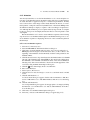
3.2 PMPATH Modeling Environment . . . . . . . . . . . . . . . . . . . . . . . . . . . . .
3.2.1 Viewing Window and cross-section windows . . . . . . . . . . . . .
3.2.2 Status bar . . . . . . . . . . . . . . . . . . . . . . . . . . . . . . . . . . . . . . . . . . .
3.2.3 Tool bar . . . . . . . . . . . . . . . . . . . . . . . . . . . . . . . . . . . . . . . . . . . .
3.2.3.1 Open model . . . . . . . . . . . . . . . . . . . . . . . . . . . . . . . . .
141
141
144
147
149
151
171
172
172
173
176
176
176
177
177
178
183
184
184
184
187
188
188
191
191
192
192
193
193
194
194
196
203
204
207
207
208
208
210
210
210
Contents
3.2.3.2 Set particle . . . . . . . . . . . . . . . . . . . . . . . . . . . . . . . . .
3.2.3.3 Erase Particle . . . . . . . . . . . . . . . . . . . . . . . . . . . . . . .
3.2.3.4 Zoom In . . . . . . . . . . . . . . . . . . . . . . . . . . . . . . . . . . . .
3.2.3.5 Zoom Out . . . . . . . . . . . . . . . . . . . . . . . . . . . . . . . . . .
3.2.3.6 Particle Color . . . . . . . . . . . . . . . . . . . . . . . . . . . . . . .
3.2.3.7 Run Particles Backward . . . . . . . . . . . . . . . . . . . . . . .
3.2.3.8 Run Particles Backward Step by Step . . . . . . . . . . .
3.2.3.9 Stop Particle Tracking . . . . . . . . . . . . . . . . . . . . . . . .
3.2.3.10 Run Particles Forward Step by Step . . . . . . . . . . . . .
3.2.3.11 Run Particles Forward . . . . . . . . . . . . . . . . . . . . . . . .
PMPATH Options Menu . . . . . . . . . . . . . . . . . . . . . . . . . . . . . . . . . . . . .
3.3.1 Environment . . . . . . . . . . . . . . . . . . . . . . . . . . . . . . . . . . . . . . . .
3.3.2 Particle Tracking (Time) . . . . . . . . . . . . . . . . . . . . . . . . . . . . . .
3.3.3 Maps . . . . . . . . . . . . . . . . . . . . . . . . . . . . . . . . . . . . . . . . . . . . . .
PMPATH Output Files . . . . . . . . . . . . . . . . . . . . . . . . . . . . . . . . . . . . . .
3.4.1 Plots . . . . . . . . . . . . . . . . . . . . . . . . . . . . . . . . . . . . . . . . . . . . . . .
3.4.2 Hydraulic Heads . . . . . . . . . . . . . . . . . . . . . . . . . . . . . . . . . . . . .
3.4.3 Drawdowns . . . . . . . . . . . . . . . . . . . . . . . . . . . . . . . . . . . . . . . . .
3.4.4 Flow Velocities . . . . . . . . . . . . . . . . . . . . . . . . . . . . . . . . . . . . . .
3.4.5 Particles . . . . . . . . . . . . . . . . . . . . . . . . . . . . . . . . . . . . . . . . . . . .
211
213
213
213
214
214
214
214
214
215
215
215
219
223
224
224
225
225
225
225
Tutorials . . . . . . . . . . . . . . . . . . . . . . . . . . . . . . . . . . . . . . . . . . . . . . . . . . . . . .
4.1 Your First Groundwater Model with PM . . . . . . . . . . . . . . . . . . . . . . .
4.1.1 Overview of the Hypothetical Problem . . . . . . . . . . . . . . . . . .
4.1.2 Run a Steady-State Flow Simulation . . . . . . . . . . . . . . . . . . . .
4.1.2.1 Step 1: Create a New Model . . . . . . . . . . . . . . . . . . .
4.1.2.2 Step 2: Assign Model Data . . . . . . . . . . . . . . . . . . . .
4.1.2.3 Step 3: Perform the Flow Simulation . . . . . . . . . . . .
4.1.2.4 Step 4: Check Simulation Results . . . . . . . . . . . . . . .
4.1.2.5 Step 5: Calculate subregional water budget . . . . . . .
4.1.2.6 Step 6: Produce Output . . . . . . . . . . . . . . . . . . . . . . .
4.1.3 Simulation of Solute Transport . . . . . . . . . . . . . . . . . . . . . . . . .
4.1.3.1 Perform Transport Simulation with MT3DMS . . . .
4.1.3.2 Perform Transport Simulation with MOC3D . . . . .
4.1.4 Parameter Estimation . . . . . . . . . . . . . . . . . . . . . . . . . . . . . . . . .
4.1.4.1 Parameter Estimation with PEST . . . . . . . . . . . . . . .
4.1.5 Animation . . . . . . . . . . . . . . . . . . . . . . . . . . . . . . . . . . . . . . . . . .
4.2 Unconfined Aquifer System with Recharge . . . . . . . . . . . . . . . . . . . . .
4.2.1 Overview of the Hypothetical Problem . . . . . . . . . . . . . . . . . .
4.2.2 Steady-state Flow Simulation . . . . . . . . . . . . . . . . . . . . . . . . . .
4.2.2.1 Step1: Create a New Model . . . . . . . . . . . . . . . . . . . .
4.2.2.2 Step2: Generate the Model Grid . . . . . . . . . . . . . . . .
4.2.2.3 Step 3: Refine the Model Grid . . . . . . . . . . . . . . . . .
4.2.2.4 Step 4: Assign Model Data . . . . . . . . . . . . . . . . . . . .
4.2.2.5 Step 5: Perform steady-state flow simulation . . . . .
227
227
227
229
229
229
237
238
239
242
249
250
257
263
265
269
271
271
272
272
272
273
274
279
3.3
3.4
4
IX
X
Contents
4.2.2.6 Step 6: Extract and view results . . . . . . . . . . . . . . . .
4.2.3 Transient Flow Simulation . . . . . . . . . . . . . . . . . . . . . . . . . . . .
Aquifer System with River . . . . . . . . . . . . . . . . . . . . . . . . . . . . . . . . . . .
4.3.1 Overview of the Hypothetical Problem . . . . . . . . . . . . . . . . . .
4.3.1.1 Step 1: Create a New Model . . . . . . . . . . . . . . . . . . .
4.3.1.2 Step 2: Generate the Model Grid . . . . . . . . . . . . . . .
4.3.1.3 Step 3: Refine the Model Grid . . . . . . . . . . . . . . . . .
4.3.1.4 Step 4: Assign Model Data . . . . . . . . . . . . . . . . . . . .
4.3.1.5 Step 5: Perform steady-state flow simulation . . . . .
4.3.1.6 Step 6: Extract and view results . . . . . . . . . . . . . . . .
279
280
284
284
285
285
286
287
293
293
Examples and Applications . . . . . . . . . . . . . . . . . . . . . . . . . . . . . . . . . . . . . .
5.1 Basic Flow Problems . . . . . . . . . . . . . . . . . . . . . . . . . . . . . . . . . . . . . . .
5.1.1 Determination of Catchment Areas . . . . . . . . . . . . . . . . . . . . .
5.1.2 Use of the General-Head Boundary Condition . . . . . . . . . . . .
5.1.3 Two-layer Aquifer System in which the Top layer Converts
between Wet and Dry . . . . . . . . . . . . . . . . . . . . . . . . . . . . . . . . .
5.1.4 Water-Table Mount resulting from Local Recharge . . . . . . . .
5.1.5 Perched Water Table . . . . . . . . . . . . . . . . . . . . . . . . . . . . . . . . . .
5.1.6 An Aquifer System with Irregular Recharge and a Stream . .
5.1.7 Flood in a River . . . . . . . . . . . . . . . . . . . . . . . . . . . . . . . . . . . . .
5.1.8 Simulation of Lakes . . . . . . . . . . . . . . . . . . . . . . . . . . . . . . . . . .
5.2 EPA Instructional Problems . . . . . . . . . . . . . . . . . . . . . . . . . . . . . . . . . .
5.3 Parameter Estimation and Pumping Test . . . . . . . . . . . . . . . . . . . . . . .
5.3.1 Basic Parameter Estimation Skill . . . . . . . . . . . . . . . . . . . . . . .
5.3.2 Estimation of Pumping Rates . . . . . . . . . . . . . . . . . . . . . . . . . .
5.3.3 The Theis Solution – Transient Flow to a Well in a
Confined Aquifer . . . . . . . . . . . . . . . . . . . . . . . . . . . . . . . . . . . .
5.3.4 The Hantush and Jacob Solution – Transient Flow to a Well
in a Leaky Confined Aquifer . . . . . . . . . . . . . . . . . . . . . . . . . . .
5.3.5 Parameter Estimation with MODFLOW-2000: Test Case 1 .
5.3.6 Parameter Estimation with MODFLOW-2000: Test Case 2 .
5.4 Geotechnical Problems . . . . . . . . . . . . . . . . . . . . . . . . . . . . . . . . . . . . . .
5.4.1 Inflow of Water into an Excavation Pit . . . . . . . . . . . . . . . . . . .
5.4.2 Flow Net and Seepage under a Weir . . . . . . . . . . . . . . . . . . . . .
5.4.3 Seepage Surface through a Dam . . . . . . . . . . . . . . . . . . . . . . . .
5.4.4 Cutoff Wall . . . . . . . . . . . . . . . . . . . . . . . . . . . . . . . . . . . . . . . . .
5.4.5 Compaction and Subsidence . . . . . . . . . . . . . . . . . . . . . . . . . . .
5.5 Solute Transport . . . . . . . . . . . . . . . . . . . . . . . . . . . . . . . . . . . . . . . . . . .
5.5.1 One-dimensional Dispersive Transport . . . . . . . . . . . . . . . . . .
5.5.2 Two-dimensional Transport in a Uniform Flow Field . . . . . .
5.5.3 Monod Kinetics . . . . . . . . . . . . . . . . . . . . . . . . . . . . . . . . . . . . .
5.5.4 Instantaneous Aerobic Biodegradation . . . . . . . . . . . . . . . . . .
5.5.5 First-Order Parent-Daughter Chain Reactions . . . . . . . . . . . . .
297
297
297
301
4.3
5
303
305
308
311
314
317
320
321
321
325
328
331
334
337
340
340
342
344
348
351
354
354
356
359
361
363
Contents
XI
5.5.6
Benchmark Problems and Application Examples from
Literature . . . . . . . . . . . . . . . . . . . . . . . . . . . . . . . . . . . . . . . . . . .
PHT3D Examples . . . . . . . . . . . . . . . . . . . . . . . . . . . . . . . . . . . . . . . . . .
SEAWAT Examples . . . . . . . . . . . . . . . . . . . . . . . . . . . . . . . . . . . . . . . .
Miscellaneous Topics . . . . . . . . . . . . . . . . . . . . . . . . . . . . . . . . . . . . . . .
5.8.1 Using the Field Interpolator . . . . . . . . . . . . . . . . . . . . . . . . . . .
5.8.2 An Example of Stochastic Modeling . . . . . . . . . . . . . . . . . . . .
365
367
368
369
369
372
Supplementary Information . . . . . . . . . . . . . . . . . . . . . . . . . . . . . . . . . . . . .
6.1 Limitation of PM . . . . . . . . . . . . . . . . . . . . . . . . . . . . . . . . . . . . . . . . . .
6.1.1 Data Editor . . . . . . . . . . . . . . . . . . . . . . . . . . . . . . . . . . . . . . . . .
6.1.2 Boreholes and Observations . . . . . . . . . . . . . . . . . . . . . . . . . . .
6.1.3 Digitizer . . . . . . . . . . . . . . . . . . . . . . . . . . . . . . . . . . . . . . . . . . . .
6.1.4 Field Interpolator . . . . . . . . . . . . . . . . . . . . . . . . . . . . . . . . . . . .
6.1.5 Field Generator . . . . . . . . . . . . . . . . . . . . . . . . . . . . . . . . . . . . . .
6.1.6 Water Budget Calculator . . . . . . . . . . . . . . . . . . . . . . . . . . . . . .
6.2 File Formats . . . . . . . . . . . . . . . . . . . . . . . . . . . . . . . . . . . . . . . . . . . . . . .
6.2.1 ASCII Matrix File . . . . . . . . . . . . . . . . . . . . . . . . . . . . . . . . . . .
6.2.2 Contour Table File . . . . . . . . . . . . . . . . . . . . . . . . . . . . . . . . . . .
6.2.3 Grid Specification File . . . . . . . . . . . . . . . . . . . . . . . . . . . . . . . .
6.2.4 Line Map File . . . . . . . . . . . . . . . . . . . . . . . . . . . . . . . . . . . . . . .
6.2.5 ASCII Time Parameter File . . . . . . . . . . . . . . . . . . . . . . . . . . . .
6.2.6 Head/Drawdown/Concentration Observation Files . . . . . . . . .
6.2.6.1 Observation Boreholes File . . . . . . . . . . . . . . . . . . . .
6.2.6.2 Layer Proportions File . . . . . . . . . . . . . . . . . . . . . . . .
6.2.6.3 Observations File . . . . . . . . . . . . . . . . . . . . . . . . . . . .
6.2.6.4 Complete Information File . . . . . . . . . . . . . . . . . . . .
6.2.7 Flow Observation Files . . . . . . . . . . . . . . . . . . . . . . . . . . . . . . .
6.2.7.1 Cell Group File . . . . . . . . . . . . . . . . . . . . . . . . . . . . . .
6.2.7.2 Flow Observations Data File . . . . . . . . . . . . . . . . . . .
6.2.7.3 Complete Information File . . . . . . . . . . . . . . . . . . . .
6.2.8 Trace File . . . . . . . . . . . . . . . . . . . . . . . . . . . . . . . . . . . . . . . . . .
6.2.9 Polygon File . . . . . . . . . . . . . . . . . . . . . . . . . . . . . . . . . . . . . . . .
6.2.10 XYZ File . . . . . . . . . . . . . . . . . . . . . . . . . . . . . . . . . . . . . . . . . . .
6.2.11 Pathline File . . . . . . . . . . . . . . . . . . . . . . . . . . . . . . . . . . . . . . . .
6.2.11.1 PMPATH Format . . . . . . . . . . . . . . . . . . . . . . . . . . . .
6.2.11.2 MODPATH Format . . . . . . . . . . . . . . . . . . . . . . . . . .
6.2.12 Particles File . . . . . . . . . . . . . . . . . . . . . . . . . . . . . . . . . . . . . . . .
6.3 Input Data Files of the supported Model . . . . . . . . . . . . . . . . . . . . . . . .
6.3.1 Name File . . . . . . . . . . . . . . . . . . . . . . . . . . . . . . . . . . . . . . . . . .
6.3.2 MODFLOW-96 . . . . . . . . . . . . . . . . . . . . . . . . . . . . . . . . . . . . .
6.3.3 MODFLOW-2000/-2005 . . . . . . . . . . . . . . . . . . . . . . . . . . . . . .
6.3.4 MODPATH and MODPATH-PLOT (version 1.x) . . . . . . . . . .
6.3.5 MODPATH and MODPATH-PLOT (version 3.x) . . . . . . . . . .
6.3.6 MOC3D . . . . . . . . . . . . . . . . . . . . . . . . . . . . . . . . . . . . . . . . . . . .
375
375
375
375
375
376
376
376
376
376
377
378
379
379
380
381
381
381
382
382
383
383
384
384
385
387
387
387
388
388
389
389
392
393
393
394
394
5.6
5.7
5.8
6
XII
Contents
6.3.7 MT3D . . . . . . . . . . . . . . . . . . . . . . . . . . . . . . . . . . . . . . . . . . . . .
6.3.8 MT3DMS/SEAWAT . . . . . . . . . . . . . . . . . . . . . . . . . . . . . . . . .
6.3.9 RT3D . . . . . . . . . . . . . . . . . . . . . . . . . . . . . . . . . . . . . . . . . . . . . .
6.3.10 PHT3D . . . . . . . . . . . . . . . . . . . . . . . . . . . . . . . . . . . . . . . . . . . .
6.3.11 PEST . . . . . . . . . . . . . . . . . . . . . . . . . . . . . . . . . . . . . . . . . . . . . .
6.4 Using MODPATH with PM . . . . . . . . . . . . . . . . . . . . . . . . . . . . . . . . . .
6.5 Define PHT3D Reaction Module . . . . . . . . . . . . . . . . . . . . . . . . . . . . . .
394
394
395
395
395
396
397
References . . . . . . . . . . . . . . . . . . . . . . . . . . . . . . . . . . . . . . . . . . . . . . . . . . . . . . . . . 399
Index . . . . . . . . . . . . . . . . . . . . . . . . . . . . . . . . . . . . . . . . . . . . . . . . . . . . . . . . . . . . . 407
List of Figures
2.1
2.2
2.3
2.4
2.5
2.6
2.7
2.8
2.9
2.10
2.11
2.12
2.13
2.14
2.15
2.16
2.17
2.18
2.19
2.20
2.21
2.22
2.23
2.24
2.25
2.26
2.27
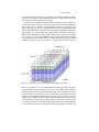
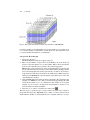
Spatial discretization of an aquifer system and the cell incides . . . . . .
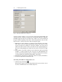
The Model Dimension dialog box . . . . . . . . . . . . . . . . . . . . . . . . . . . . . .
The Grid Editor . . . . . . . . . . . . . . . . . . . . . . . . . . . . . . . . . . . . . . . . . . . . .
The Grid Size dialog box . . . . . . . . . . . . . . . . . . . . . . . . . . . . . . . . . . . . .
The Data Editor (Grid View) . . . . . . . . . . . . . . . . . . . . . . . . . . . . . . . . . .
The Data Editor (Map View) . . . . . . . . . . . . . . . . . . . . . . . . . . . . . . . . . .
The Data Editor (Cross-sectional View) . . . . . . . . . . . . . . . . . . . . . . . . .
The Cell Information dialog box . . . . . . . . . . . . . . . . . . . . . . . . . . . . . . .
The Search and Modify Cell Values dialog box . . . . . . . . . . . . . . . . . . .
The Temporal Data dialog box . . . . . . . . . . . . . . . . . . . . . . . . . . . . . . . .
The Convert Model dialog box . . . . . . . . . . . . . . . . . . . . . . . . . . . . . . . .
Telescoping a flow model using the Convert Model dialog box . . . . . .
The Preferences dialog box . . . . . . . . . . . . . . . . . . . . . . . . . . . . . . . . . . .
The Layer Property dialog box . . . . . . . . . . . . . . . . . . . . . . . . . . . . . . . .
Grid configuration used for the calculation of VCONT . . . . . . . . . . . .
The Time Parameters dialog box for MODFLOW2000/MODFLOW-2005 . . . . . . . . . . . . . . . . . . . . . . . . . . . . . . . . . . . . . .
The Time Parameters dialog box for MODFLOW-96 . . . . . . . . . . . . . .
The Drain Parameters dialog box . . . . . . . . . . . . . . . . . . . . . . . . . . . . . .
The General Head Boundary Parameters dialog box . . . . . . . . . . . . . . .
The Horizontal-Flow Barrier dialog box . . . . . . . . . . . . . . . . . . . . . . . . .
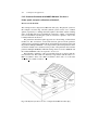
Types of fine-grained beds in or adjacent to aquifers. Beds may
be discontinuous interbeds or continuous confining beds. Adapted
from Leake and Prudic [78]. . . . . . . . . . . . . . . . . . . . . . . . . . . . . . . . . . .
The Recharge Package dialog box . . . . . . . . . . . . . . . . . . . . . . . . . . . . . .
The Reservoir Package dialog box . . . . . . . . . . . . . . . . . . . . . . . . . . . . .
The Stage-Time Table of Reservoirs dialog box . . . . . . . . . . . . . . . . . .
The River Parameters dialog box . . . . . . . . . . . . . . . . . . . . . . . . . . . . . . .
The Stream Parameters dialog box . . . . . . . . . . . . . . . . . . . . . . . . . . . . .
Specification of the stream structure . . . . . . . . . . . . . . . . . . . . . . . . . . . .
9
10
11
13
14
14
16
17
17
21
22
23
23
28
30
34
34
39
42
44
45
48
50
50
52
54
57
XIV
List of Figures
2.28
2.29
2.30
2.31
2.32
2.33
2.34
2.35
2.36
2.37
2.38
2.39
2.40
2.41
2.42
2.43
2.44
2.45
2.46
2.47
2.48
2.49
2.50
2.51
2.52
2.53
2.54
2.55
2.56
2.57
2.58
2.59
2.60
2.61
2.62
The stream system configured by the table of Fig. 2.27 . . . . . . . . . . . .
The Wetting Capability dialog box . . . . . . . . . . . . . . . . . . . . . . . . . . . . .
The Direct Solution (DE45) dialog box . . . . . . . . . . . . . . . . . . . . . . . . .
The Preconditioned Conjugate Gradient Package 2 dialog box . . . . . .
The Strongly Implicit Procedure Package dialog box . . . . . . . . . . . . . .
The Slice-Successive Overrelaxation Package dialog box . . . . . . . . . .
The Geometric Multigrid Solver dialog box . . . . . . . . . . . . . . . . . . . . .
The Head Observation dialog box . . . . . . . . . . . . . . . . . . . . . . . . . . . . . .
The Modflow Output Control dialog box . . . . . . . . . . . . . . . . . . . . . . . .
The Run Modflow dialog box . . . . . . . . . . . . . . . . . . . . . . . . . . . . . . . . .
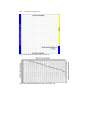
The Data tab of the Scatter Diagram (Hydraulic Head) dialog box . . .
Interpolation of simulated head values to an observation borehole . . .
The Chart tab of the Scatter Diagram (Hydraulic Head) dialog box . .
The Data tab of the Time Series Curves (Hydraulic Head) dialog box
The Chart tab of the Head-Time Series Curves Diagram dialog box . .
The Initial Concentration dialog box . . . . . . . . . . . . . . . . . . . . . . . . . . . .
The Simulation Settings (MT3DMS/SEAWAT) dialog box . . . . . . . . .
The Stoichiometry tab of the Simulation Settings
(MT3DMS/SEAWAT) dialog box . . . . . . . . . . . . . . . . . . . . . . . . . . . . . .
The Variable Density tab of the Simulation Settings
(MT3DMS/SEAWAT) dialog box . . . . . . . . . . . . . . . . . . . . . . . . . . . . . .
The Advection Package (MT3DMS) dialog box . . . . . . . . . . . . . . . . . .
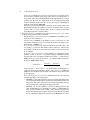
Initial placement of moving particles (adapted from Zheng [117]):
(a) Fixed pattern, 8 particles are placed on two planes within a cell.
(b) Random pattern, 8 particles are placed randomly within a cell. . . .
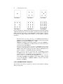
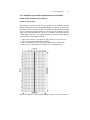
Distribution of initial particles using the fixed pattern (adapted from
Zheng 1990) If the fixed pattern is chosen, the number of particles
placed per cell (NPL and NPH) is divided by the number of planes
NPLANE to yield the number of particles to be placed on each
plane, which is then rounded to one of the numbers of particles
shown here. . . . . . . . . . . . . . . . . . . . . . . . . . . . . . . . . . . . . . . . . . . . . . . . .
The Dispersion Package dialog box . . . . . . . . . . . . . . . . . . . . . . . . . . . .
The Chemical Reaction (MT3DMS) dialog box . . . . . . . . . . . . . . . . . .
The Generalized Conjugate Gradient (GCG) dialog box . . . . . . . . . . .
The Output Control (MT3D/MT3DMS) dialog box . . . . . . . . . . . . . . .
The Output Times tab of the Output Control (MT3D/MT3DMS)
dialog box . . . . . . . . . . . . . . . . . . . . . . . . . . . . . . . . . . . . . . . . . . . . . . . . .
The Run MT3DMS dialog box . . . . . . . . . . . . . . . . . . . . . . . . . . . . . . . .
The Run SEAWAT dialog box . . . . . . . . . . . . . . . . . . . . . . . . . . . . . . . . .
The Chemical Reaction Module (PHT3D) dialog box . . . . . . . . . . . . .
The Simulation Settings (PHT3D) dialog box . . . . . . . . . . . . . . . . . . . .
The Reaction Definition (RT3D) dialog box . . . . . . . . . . . . . . . . . . . . .
The Sorption Parameters (RT3D) dialog box . . . . . . . . . . . . . . . . . . . . .
The Reaction Parameters for RT3D (Spatially Constant) dialog box .
The Run RT3D dialog box . . . . . . . . . . . . . . . . . . . . . . . . . . . . . . . . . . . .
57
61
63
65
67
68
69
71
74
76
78
79
80
82
83
84
85
87
89
90
93
94
95
97
103
105
106
106
107
110
110
113
115
116
117
List of Figures
2.63
2.64
2.65
2.66
2.67
2.68
2.69
2.70
2.71
2.72
The Subgrid for Transport (MOC3D) dialog box . . . . . . . . . . . . . . . . .
The Parameter for Advective Transport (MOC3D) dialog box . . . . . .
The Dispersion / Chemical Reaction (MOC3D) dialog box . . . . . . . . .
The Source Concentration (Constant Head) dialog box . . . . . . . . . . . .
The Output Control (MOC3D) dialog box . . . . . . . . . . . . . . . . . . . . . . .
The Run Moc3d dialog box . . . . . . . . . . . . . . . . . . . . . . . . . . . . . . . . . . .
The Advection Package (MTADV1) dialog box . . . . . . . . . . . . . . . . . .
The Chemical Reaction Package (MTRCT1) dialog box . . . . . . . . . . .
The Output Control (MT3D/MT3DMS) dialog box . . . . . . . . . . . . . . .
The Output Times tab of the Output Control (MT3D/MT3DMS)
dialog box . . . . . . . . . . . . . . . . . . . . . . . . . . . . . . . . . . . . . . . . . . . . . . . . .
2.73 The Run MT3D/MT3D96 dialog box . . . . . . . . . . . . . . . . . . . . . . . . . . .
2.74 The Simulation Settings (MODFLOW-2000) dialog box . . . . . . . . . . .
2.75 The Flow Observation (River) dialog box . . . . . . . . . . . . . . . . . . . . . . .
2.76 The Flow Observation tab of the Flow Observation (River) dialog box
2.77 The Run MODFLOW-2000 (Sensitivity Analysis/Parameter
Estimation) dialog box . . . . . . . . . . . . . . . . . . . . . . . . . . . . . . . . . . . . . . .
2.78 The Run PEST-ASP + MODFLOW-2000 dialog box . . . . . . . . . . . . . .
2.79 The Simulation Settings (PEST) dialog box . . . . . . . . . . . . . . . . . . . . . .
2.80 The Parameter Groups tab of the Simulation Settings (PEST) dialog
box . . . . . . . . . . . . . . . . . . . . . . . . . . . . . . . . . . . . . . . . . . . . . . . . . . . . . . .
2.81 The Regularization tab of the Simulation Settings (PEST) dialog box
2.82 The SVD/SVD-Assist tab of the Simulation Settings (PEST) dialog
box . . . . . . . . . . . . . . . . . . . . . . . . . . . . . . . . . . . . . . . . . . . . . . . . . . . . . . .
2.83 The Control Data tab of the Simulation Settings (PEST) dialog box . .
2.84 The Run PEST dialog box . . . . . . . . . . . . . . . . . . . . . . . . . . . . . . . . . . . .
2.85 The Field Interpolator dialog box . . . . . . . . . . . . . . . . . . . . . . . . . . . . . .
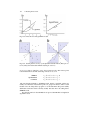
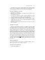
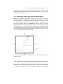
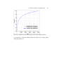
2.86 Effects of different weighting exponents . . . . . . . . . . . . . . . . . . . . . . . .
2.87 The Variogram dialog box . . . . . . . . . . . . . . . . . . . . . . . . . . . . . . . . . . . .
2.88 Linear, Power and logarithmic models . . . . . . . . . . . . . . . . . . . . . . . . . .
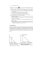
2.89 Search patterns used by (a) the Quadrant Search method (Data per
sector=2) and (b) the Octant Search method (Data per sector=1) . . . .
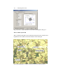
2.90 The Field Generator dialog box . . . . . . . . . . . . . . . . . . . . . . . . . . . . . . . .
2.91 The 2D Visualization tool in action . . . . . . . . . . . . . . . . . . . . . . . . . . . . .
2.92 The Result Selection dialog box . . . . . . . . . . . . . . . . . . . . . . . . . . . . . . .
2.93 The Results Extractor dialog box . . . . . . . . . . . . . . . . . . . . . . . . . . . . . .
2.94 The Water Budget dialog box . . . . . . . . . . . . . . . . . . . . . . . . . . . . . . . . .
2.95 The Browse Matrix dialog box . . . . . . . . . . . . . . . . . . . . . . . . . . . . . . . .
2.96 The Load Matrix dialog box . . . . . . . . . . . . . . . . . . . . . . . . . . . . . . . . . .
2.97 The starting position of a loaded ASCII matrix . . . . . . . . . . . . . . . . . . .
2.98 The Reset Matrix dialog box . . . . . . . . . . . . . . . . . . . . . . . . . . . . . . . . . .
2.99 The Search and Modify dialog box . . . . . . . . . . . . . . . . . . . . . . . . . . . . .
2.100The Import Results dialog box . . . . . . . . . . . . . . . . . . . . . . . . . . . . . . . . .
2.101The Map Options dialog box . . . . . . . . . . . . . . . . . . . . . . . . . . . . . . . . . .
2.102Scaling a vector graphic . . . . . . . . . . . . . . . . . . . . . . . . . . . . . . . . . . . . . .
XV
119
120
122
123
124
125
127
131
132
133
134
137
142
143
144
146
152
155
160
163
168
172
178
180
181
182
182
183
185
185
186
188
190
190
191
191
192
193
194
196
XVI
List of Figures
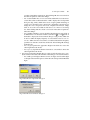
2.103Importing and Geo-referencing a raster map . . . . . . . . . . . . . . . . . . . . .
2.104The Appearance tab of the Environment Options dialog box . . . . . . . .
2.105The Coordinate System tab of the Environment Options dialog box . .
2.106Defining the coordinate system and orientation of the model grid . . . .
2.107The Contours tab of the Environment Options dialog box . . . . . . . . . .
2.108The Color Spectrum dialog box . . . . . . . . . . . . . . . . . . . . . . . . . . . . . . . .
2.109The Contour Labels dialog box . . . . . . . . . . . . . . . . . . . . . . . . . . . . . . . .
2.110The Label Format dialog box . . . . . . . . . . . . . . . . . . . . . . . . . . . . . . . . . .
3.1
3.2
197
197
198
198
200
201
201
202
3.8
3.9
3.10
3.11
3.12
3.13
3.14
3.15
3.16
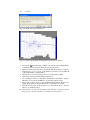
PMPATH in action . . . . . . . . . . . . . . . . . . . . . . . . . . . . . . . . . . . . . . . . . . 204
(a) Flow through an infinitesimal volume of a porous medium and
(b) the finite-difference approach . . . . . . . . . . . . . . . . . . . . . . . . . . . . . . 204
Schematic illustration of the spurious intersection of two pathlines
in a two-dimensional cell . . . . . . . . . . . . . . . . . . . . . . . . . . . . . . . . . . . . . 207
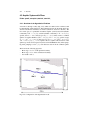
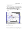
The PMPATH modeling environment . . . . . . . . . . . . . . . . . . . . . . . . . . . 209
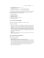
The Add New Particles dialog box . . . . . . . . . . . . . . . . . . . . . . . . . . . . . 212
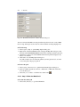
The Environment Options dialog box of PMPATH . . . . . . . . . . . . . . . . 215
The Cross Sections tab of the Environment Options dialog box of
PMPATH . . . . . . . . . . . . . . . . . . . . . . . . . . . . . . . . . . . . . . . . . . . . . . . . . . 216
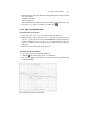
The Contours tab of the Environment Options dialog box of PMPATH 217
The Color Spectrum dialog box . . . . . . . . . . . . . . . . . . . . . . . . . . . . . . . . 218
The Contour Labels dialog box . . . . . . . . . . . . . . . . . . . . . . . . . . . . . . . . 218
The Label Format dialog box . . . . . . . . . . . . . . . . . . . . . . . . . . . . . . . . . . 219
The Particle Tracking (Time) dialog box . . . . . . . . . . . . . . . . . . . . . . . . 220
The Pathline Colors tab of the Particle Tracking (Time) dialog box . . 222
The RCH/EVT Options tab of the Particle Tracking (Time) dialog box 222
The Maps Options dialog box . . . . . . . . . . . . . . . . . . . . . . . . . . . . . . . . . 223
The Save Plot As dialog box . . . . . . . . . . . . . . . . . . . . . . . . . . . . . . . . . . 224
4.1
4.2
4.3
4.4
4.5
4.6
4.7
4.8
4.9
4.10
4.11
4.12
4.13
4.14
4.15
4.16
Configuration of the hypothetical model . . . . . . . . . . . . . . . . . . . . . . . .
The spatial discretization scheme and cell indices of MODFLOW . . .
The Model Dimension dialog box . . . . . . . . . . . . . . . . . . . . . . . . . . . . . .
The generated model grid . . . . . . . . . . . . . . . . . . . . . . . . . . . . . . . . . . . . .
The Layer Options dialog box and the layer type drop-down list . . . .
The Data Editor displaying the plan view of the model grid . . . . . . . .
The Run Modflow dialog box . . . . . . . . . . . . . . . . . . . . . . . . . . . . . . . . .
The Water Budget dialog box . . . . . . . . . . . . . . . . . . . . . . . . . . . . . . . . .
The Results Extractor dialog box . . . . . . . . . . . . . . . . . . . . . . . . . . . . . .
The Result Selection dialog box . . . . . . . . . . . . . . . . . . . . . . . . . . . . . . .
Contours of the hydraulic heads in the first layer . . . . . . . . . . . . . . . . . .
The model loaded in PMPATH . . . . . . . . . . . . . . . . . . . . . . . . . . . . . . . .
The Add New Particles dialog box . . . . . . . . . . . . . . . . . . . . . . . . . . . . .
The capture zone of the pumping well (vertical exaggeration = 1) . . .
The capture zone of the pumping well (vertical exaggeration = 10) . .
The 100-day capture zone calculated by PMPATH . . . . . . . . . . . . . . . .
3.3
3.4
3.5
3.6
3.7
228
230
231
231
232
234
238
240
243
244
245
246
247
247
248
248
List of Figures
4.17
4.18
4.19
4.20
4.21
4.22
4.23
4.24
4.25
4.26
4.27
4.28
4.29
4.30
4.31
4.32
4.33
4.34
4.35
4.36
4.37
4.38
4.39
4.40
4.41
4.42
4.43
4.44
4.45
4.46
4.47
4.48
4.49
4.50
4.51
4.52
4.53
4.54
4.55
4.56
4.57
4.58
The Particle Tracking (Time) Properties dialog box . . . . . . . . . . . . . . .
The Concentration Observation dialog box . . . . . . . . . . . . . . . . . . . . . .
The Reaction Definition dialog box . . . . . . . . . . . . . . . . . . . . . . . . . . . .
The Advection Package (MT3DMS) dialog box . . . . . . . . . . . . . . . . . .
The Dispersion Package (MT3D/MT3DMS/RT3D) dialog box . . . . .
The Reset Matrix dialog box for chemical reaction data of MT3DMS
The Output Control (MT3D Family) dialog box . . . . . . . . . . . . . . . . . .
The Run MT3DMS dialog box . . . . . . . . . . . . . . . . . . . . . . . . . . . . . . . .
Contours of the concentration values at the end of the simulation . . . .
The Time Series Curves (Concentration) dialog box . . . . . . . . . . . . . . .
The Chart tab of the Time Series Curves (Concentration) dialog box .
The Subgrid for Transport (MOC3D) dialog box . . . . . . . . . . . . . . . . .
The Parameters for Advective Transport (MOC3D) dialog box . . . . . .
The Dispersion / Chemical Reaction (MOC3D) dialog box . . . . . . . . .
The Output Control (MOC3D) dialog box . . . . . . . . . . . . . . . . . . . . . . .
The Run Moc3d dialog box . . . . . . . . . . . . . . . . . . . . . . . . . . . . . . . . . . .
Contours of the concentration values at the end of the simulation . . . .
The Time Series Curves (Concentration) dialog box . . . . . . . . . . . . . . .
The Chart tab of the Time Series Curves (Concentration) dialog box .
The Head Observation dialog box . . . . . . . . . . . . . . . . . . . . . . . . . . . . . .
The List of Parameters (PEST) dialog box . . . . . . . . . . . . . . . . . . . . . . .
The Run PEST dialog box . . . . . . . . . . . . . . . . . . . . . . . . . . . . . . . . . . . .
The Scatter Diagram dialog box . . . . . . . . . . . . . . . . . . . . . . . . . . . . . . .
The Chart tab of the Scatter Diagram dialog box . . . . . . . . . . . . . . . . . .
The Animation dialog box . . . . . . . . . . . . . . . . . . . . . . . . . . . . . . . . . . . .
Configuration of the hypothetical model . . . . . . . . . . . . . . . . . . . . . . . .
The Model Grid and Coordinate System dialog box . . . . . . . . . . . . . . .
Model grid after the refinement . . . . . . . . . . . . . . . . . . . . . . . . . . . . . . . .
Model Boundaries . . . . . . . . . . . . . . . . . . . . . . . . . . . . . . . . . . . . . . . . . . .
Steady state head distribution . . . . . . . . . . . . . . . . . . . . . . . . . . . . . . . . .
(a) Head distribution after 240 days of pumping (period 1, time step
12) (b) Head distribution after 120 days of recharge (period 2, time
step 6) . . . . . . . . . . . . . . . . . . . . . . . . . . . . . . . . . . . . . . . . . . . . . . . . . . . . .
Configuration of the hypothetical model . . . . . . . . . . . . . . . . . . . . . . . .
The Model Grid and Coordinate System dialog box . . . . . . . . . . . . . . .
Model grid after the refinement . . . . . . . . . . . . . . . . . . . . . . . . . . . . . . . .
Model grid of the 1st layer and 3rd layer . . . . . . . . . . . . . . . . . . . . . . . .
Model grid of the 2nd layer . . . . . . . . . . . . . . . . . . . . . . . . . . . . . . . . . . .
Define the river using a polyline . . . . . . . . . . . . . . . . . . . . . . . . . . . . . . .
Parameters of the upstream vertex . . . . . . . . . . . . . . . . . . . . . . . . . . . . . .
Parameters of the downstream vertex . . . . . . . . . . . . . . . . . . . . . . . . . . .
The Result Selection dialog box . . . . . . . . . . . . . . . . . . . . . . . . . . . . . . .
Steady state hydraulic head distribution in the first model layer . . . . .
Steady state hydraulic head distribution in the 3rd model layer and
capture zones of the pumping wells . . . . . . . . . . . . . . . . . . . . . . . . . . . .
XVII
249
250
251
252
253
254
254
255
256
257
257
258
259
260
261
261
262
263
264
265
266
267
268
268
270
271
273
275
277
280
283
284
286
287
288
289
292
292
293
294
294
295
XVIII
List of Figures
4.59 125-year streamlines; particles are started at the cell [6, 5, 1] and
flow towards Well 2 . . . . . . . . . . . . . . . . . . . . . . . . . . . . . . . . . . . . . . . . . . 296
5.1
5.2
5.3
5.4
5.5
5.6
5.7
5.8
5.9
5.10
5.11
5.12
5.13
5.14
5.15
5.16
5.17
5.18
5.19
5.20
5.21
5.22
5.23
5.24
5.25
5.26
5.27
5.28
5.29
5.30
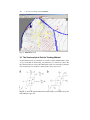
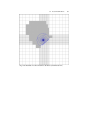
Plan view of the model area . . . . . . . . . . . . . . . . . . . . . . . . . . . . . . . . . . .
Catchment area and 365-days isochrones of the pumping well
(2D-approach: ground-water recharge is treated as distributed
source within the model cells) . . . . . . . . . . . . . . . . . . . . . . . . . . . . . . . . .
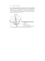
Particles are tracked back to the groundwater surface by applying
the groundwater recharge on the groundwater surface (3D-approach)
Catchment area of the pumping well (3D-approach) . . . . . . . . . . . . . . .
Plan view of the model area . . . . . . . . . . . . . . . . . . . . . . . . . . . . . . . . . . .
Calculated head contours for the west part of the aquifer . . . . . . . . . . .
Calculated head contours for the entire aquifer . . . . . . . . . . . . . . . . . . .
Configuration of the hypothetical model (after McDonald and others
[86]) . . . . . . . . . . . . . . . . . . . . . . . . . . . . . . . . . . . . . . . . . . . . . . . . . . . . . .
Hydrogeology and model grid configuration . . . . . . . . . . . . . . . . . . . . .
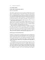
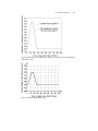
Simulated water-table along row 1 beneath a leaking pond after 190,
708, 2630 days and steady state conditions . . . . . . . . . . . . . . . . . . . . . .
Hydrogeology and model grid configuration . . . . . . . . . . . . . . . . . . . . .
Simulated steady state head distribution in layer 1 . . . . . . . . . . . . . . . .
Configuration of the model grid and the location of the observation
well . . . . . . . . . . . . . . . . . . . . . . . . . . . . . . . . . . . . . . . . . . . . . . . . . . . . . . .
Distribution of recharge used for analytical solution and the model
(after Prudic [98]) . . . . . . . . . . . . . . . . . . . . . . . . . . . . . . . . . . . . . . . . . . .
Comparison of simulation results to analytical solution developed
by Oakes and Wilkinson [90] . . . . . . . . . . . . . . . . . . . . . . . . . . . . . . . . . .
Distribution of streamflow for a 30-day flood event used for the
simulation (after Prudic [98]) . . . . . . . . . . . . . . . . . . . . . . . . . . . . . . . . . .
Model calculated river stage . . . . . . . . . . . . . . . . . . . . . . . . . . . . . . . . . .
Numbering system of streams and diversions (after Prudic [98]) . . . .
Plan and cross-sectional views of the model area . . . . . . . . . . . . . . . . .
Steady-state hydraulic head contours in layer 4 . . . . . . . . . . . . . . . . . . .
Time-series curve of the water stage in the lake . . . . . . . . . . . . . . . . . .
Configuration of the aquifer system . . . . . . . . . . . . . . . . . . . . . . . . . . . .
Plan view of the model . . . . . . . . . . . . . . . . . . . . . . . . . . . . . . . . . . . . . . .
Location of the cutoff wall and pumping wells . . . . . . . . . . . . . . . . . . .
Time series curve of the calculated hydraulic head at the center of
the contaminated area . . . . . . . . . . . . . . . . . . . . . . . . . . . . . . . . . . . . . . . .
Plan view of the model . . . . . . . . . . . . . . . . . . . . . . . . . . . . . . . . . . . . . . .
Time-series curves of the calculated and observed drawdown values .
Configuration of the leaky aquifer system and the aquifer parameters
Configuration of the leaky aquifer system and the aquifer parameters
Physical system for test case 1. Adapted from Hill and others [63] . . .
298
299
299
300
301
302
302
304
306
307
309
310
311
312
313
315
315
316
317
319
319
322
326
326
327
329
330
331
333
334
List of Figures
XIX
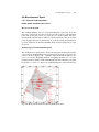
5.31 Test case 2 model grid, boundary conditions, observation locations
and hydraulic conductivity zonation used in parameter estimation.
Adapted from Hill and others [63] . . . . . . . . . . . . . . . . . . . . . . . . . . . . . 338
5.32 Configuration of the physical system . . . . . . . . . . . . . . . . . . . . . . . . . . . 341
5.33 Simulated head distribution and catchment area of the excavation pit 341
5.34 Configuration of the physical system . . . . . . . . . . . . . . . . . . . . . . . . . . . 343
5.35 Model grid and the boundary conditions . . . . . . . . . . . . . . . . . . . . . . . . 343
5.36 Flowlines and calculated head contours for isotropic medium . . . . . . . 343
5.37 Flowlines and calculated head contours for anisotropic medium . . . . . 343
5.38 Seepage surface through a dam . . . . . . . . . . . . . . . . . . . . . . . . . . . . . . . . 345
5.39 Model grid and the boundary conditions . . . . . . . . . . . . . . . . . . . . . . . . 346
5.40 Calculated hydraulic heads after one iteration step . . . . . . . . . . . . . . . . 346
5.41 Calculated hydraulic heads distribution and the form of the seepage
surface . . . . . . . . . . . . . . . . . . . . . . . . . . . . . . . . . . . . . . . . . . . . . . . . . . . . 347
5.42 Model grid and boundary conditions . . . . . . . . . . . . . . . . . . . . . . . . . . . . 349
5.43 Plan and cross-sectional views of flowlines. Particles are started
from the contaminated area. The depth of the cutoff wall is -8 m. . . . . 350
5.44 Plan and cross-sectional views of flowlines. Particles are started
from the contaminated area. The depth of the cutoff wall is -10 m . . . 350
5.45 Model grid and boundary conditions . . . . . . . . . . . . . . . . . . . . . . . . . . . . 352
5.46 Distribution of the land surface subsidence (maximum 0.11 m) . . . . . 353
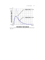
5.47 Comparison of the calculated breakthrough curves with different
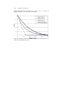
dispersivity values . . . . . . . . . . . . . . . . . . . . . . . . . . . . . . . . . . . . . . . . . . . 355
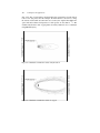
5.48 Configuration of the model and the location of an observation borehole357
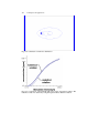
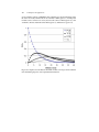
5.50 Comparison of the breakthrough curves at the observation borehole.
The numerical solution is obtained by using the 3rd order TVD
scheme. . . . . . . . . . . . . . . . . . . . . . . . . . . . . . . . . . . . . . . . . . . . . . . . . . . . . 357
5.49 Calculated concentration distribution . . . . . . . . . . . . . . . . . . . . . . . . . . . 358
5.51 Comparison of the breakthrough curves at the observation borehole.
The numerical solution is obtained by using the upstream finite
difference method. . . . . . . . . . . . . . . . . . . . . . . . . . . . . . . . . . . . . . . . . . . . 358
5.52 Calculated concentration values for one-dimensional transport from
a constant source in a uniform flow field. . . . . . . . . . . . . . . . . . . . . . . . . 360
5.53 Calculated concentration values of hydrocarbon . . . . . . . . . . . . . . . . . . 362
5.54 Calculated concentration values of oxygen . . . . . . . . . . . . . . . . . . . . . . 362
5.55 Comparison of calculated concentration values of four species in a
uniform flow field undergoing first-order sequential transformation . . 364
5.56 Model domain and the measured hydraulic head values . . . . . . . . . . . . 369
5.57 Contours produced by Shepard’s inverse distance method . . . . . . . . . . 370
5.58 Contours produced by the Kriging method . . . . . . . . . . . . . . . . . . . . . . . 370
5.59 Contours produced by Akima’s bivariate interpolation . . . . . . . . . . . . . 371
5.60 Contours produced by Renka’s triangulation algorithm . . . . . . . . . . . . 371
5.61 Calculation of the mean safety criterion by the Monte Carlo method . 373
6.1
Local coordinates within a cell . . . . . . . . . . . . . . . . . . . . . . . . . . . . . . . . 389
List of Tables
2.1
2.2
2.3
2.4
2.5
2.6
2.7
2.8
2.9
2.10
Symbols used in the present text . . . . . . . . . . . . . . . . . . . . . . . . . . . . . . .
Summary of menus in PM . . . . . . . . . . . . . . . . . . . . . . . . . . . . . . . . . . . .
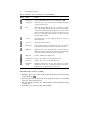
Summary of the toolbar buttons of the Grid Editor . . . . . . . . . . . . . . . .
Summary of the toolbar buttons of the Data Editor . . . . . . . . . . . . . . . .
Versions and Filenames of MODFLOW . . . . . . . . . . . . . . . . . . . . . . . . .
Model Data checked by PM . . . . . . . . . . . . . . . . . . . . . . . . . . . . . . . . . .
Names of the MOC3D output files . . . . . . . . . . . . . . . . . . . . . . . . . . . . .
Adjustable parameters through MODFLOW-2000 within PM . . . . . .
Adjustable parameters through PEST within PM . . . . . . . . . . . . . . . . .
Output from the Water Budget Calculator . . . . . . . . . . . . . . . . . . . . . . .
3.1
Summary of the toolbar buttons of PMPATH . . . . . . . . . . . . . . . . . . . . . 211
4.1
4.2
4.3
4.4
4.5
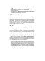
Output files from MODFLOW . . . . . . . . . . . . . . . . . . . . . . . . . . . . . . . .
Volumetric budget for the entire model written by MODFLOW . . . . .
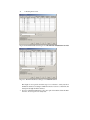
Output from the Water Budget Calculator . . . . . . . . . . . . . . . . . . . . . . .
Output from the Water Budget Calculator for the pumping well . . . . .
Measured hydraulic head values for parameter estimation . . . . . . . . . .
239
239
241
242
264
5.1
5.2
5.3
5.4
5.5
318
322
323
332
5.7
5.8
Volumetric budget for the entire model written by MODFLOW . . . . .
River data . . . . . . . . . . . . . . . . . . . . . . . . . . . . . . . . . . . . . . . . . . . . . . . . . .
Measurement data . . . . . . . . . . . . . . . . . . . . . . . . . . . . . . . . . . . . . . . . . . .
Analytical solution for the drawdown with time . . . . . . . . . . . . . . . . . .
Parameters defined for MODFLOW-2000 test case 1, parameter
values, starting and estimated PARVAL . . . . . . . . . . . . . . . . . . . . . . . . .
Parameters defined for MODFLOW-2000 test case 2, parameter
values, starting and estimated PARVAL . . . . . . . . . . . . . . . . . . . . . . . . .
PHT3D Examples . . . . . . . . . . . . . . . . . . . . . . . . . . . . . . . . . . . . . . . . . . .
SEAWAT Examples . . . . . . . . . . . . . . . . . . . . . . . . . . . . . . . . . . . . . . . . .
6.1
Assignment of parameters in the Value(I) vector . . . . . . . . . . . . . . . . . . 386
5.6
7
8
12
15
24
77
124
135
150
189
336
339
367
368
1
Introduction
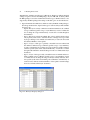
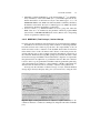
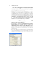
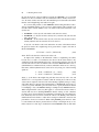
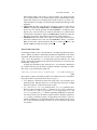
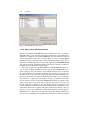
Processing Modflow (PM) was originally developed to support the first official release of MODFLOW-88 [85] to simulate the inundation process of an abandoned
open-cast coal mine. Since the release of MODFLOW-88, many computer codes
have been developed to add functionalities to MODFLOW or to use MODFLOW as a
flow-equation solver for solving specific problems. Consequently, several versions of
PM[17][22][24] have been released to utilize latest computer codes, to facilitate the
modeling process, and to free up modelers from tedious data input for more creative
thinking. The computer codes that are supported by present version of Processing
Modflow are given in the following section.
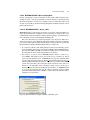
1.1 Supported Computer Codes
•
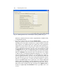
MODFLOW [85][54][55][56][63][57]
MODFLOW is a modular three-dimensional finite-difference groundwater model
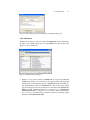
published by the U. S. Geological Survey. The first public version of MODFLOW was released in 1988 and is referred to as MODFLOW-88. MODFLOW88 and the later version of MODFLOW-96 [54][55] were originally designed
to simulate saturated three-dimensional groundwater flow through porous media. MODFLOW-2000 [56] attempts to incorporate the solution of multiple related equations into a single code. To achieve the goal, the code is divided into
entities called processes. Each process deals with a specific equation. For example, the Groundwater Flow Process (GWF) deals with the groundwater-flow
equation and replaces the original MODFLOW. The parameter estimation capability of MODFLOW-2000 is implemented by Hill and others [63] using three
processes in addition to the GWF process. The Observation Process (OBS) calculates simulated values that are to be compared to measurements, calculates
the sum of squared, weighted differences between model values and observations and calculates sensitivities related to the observations. The Sensitivity Process (SEN) solves the sensitivity equation for hydraulic heads throughout the
2
•
•
•
•
1 Introduction
grid, and the Parameter-Estimation (PES) Process solves the modified GaussNewton equation to minimize an objective function to find optimal parameter
values. Although the OBS, SEN and PES processes allow MODFLOW-2000
to perform a model calibration without the need for any external parameter estimation software, there will still be many situations in which it is preferable
to calibrate a MODFLOW model using external parameter estimation software
rather than using built-in MODFLOW-2000 parameter estimation functionality
[36]. To combine the strengths of PEST-ASP and MODFLOW-2000, a modified version of MODFLOW-2000, called MODFLOW-ASP [35], allows a coupled PEST-ASP+MODFLOW-2000 approach using MODFLOW-ASP to calculate derivatives and using PEST-ASP to estimate parameter values. The latest
major version of MODFLOW was released in 2005, called MODFLOW-2005
[57]. This version, however, does not support parameter estimation process at
the time of this writing. As a result, users are encouraged to take advantage of
external parameter-estimation programs such as PEST.
PEST [33][37][38]
The purpose of PEST is to assist in data interpretation and in parameter estimation. If there are field or laboratory measurements, PEST an adjust model parameters and/or excitation data in order that the discrepancies between the pertinent
model-generated numbers and the corresponding measurements are reduced to
a minimum. PEST does this by taking control of the model (MODFLOW) and
running it as many times as is necessary in order to determine this optimal set
of parameters and/or excitations. PEST includes many cutting-edge parameter
estimation techniques. According to Doherty [37], the most profound advance is
the ”SVD-assist” scheme. This method combines two important regularization
methodologies–”truncated singular value decomposition” and ”Tikhonov regularization”.
MODPATH [93][93][94]
MODPATH is a particle tracking code written in FORTRAN. To run a particle
tracking simulation with MODPATH, the users need to key in parameters in a
text screen and have the options to save the input values in a separate file for later
use. A graphical post-processor, such as MODPATH-PLOT [95], 3D Groundwater Explorer [21] or 3D Master[23], is required for displaying the calculated
pathlines and particle locations.
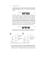
PMPATH [19]
PMPATH is a Windows-based advective transport model for calculating and
animating path lines of groundwater. PMPATH uses a semi-analytical particletracking scheme used in MODPATH [93] to calculate the groundwater paths
and travel times. PMPATH supports both forward and backward particle-tracking
schemes for steady-state and transient flow fields. The graphical user interface of
PMPATH allows the user to run a particle tracking simulation with just a few
clicks of the mouse. Pathlines or flowlines and travel time marks are calculated
and displayed along with various on-screen graphical options including head or
drawdown contours and velocity vectors.
MOC3D [74]
1.1 Supported Computer Codes
•
•
•
•
3
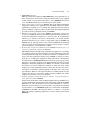
MOC3D is a single-species transport model computes changes in concentration
of a single dissolved chemical constituent over time that are caused by advective transport, hydrodynamic dispersion (including both mechanical dispersion
and diffusion), mixing or dilution from fluid sources, and mathematically simple
chemical reactions, including decay and linear sorption represented by a retardation factor. MOC3D uses the method of characteristics to solve the transport
equation on the basis of the hydraulic gradients computed with MODFLOW for
a given time step. This implementation of the method of characteristics uses particle tracking to represent advective transport and explicit finite-difference methods to calculate the effects of other processes. For improved efficiency, the user
can apply MOC3D to a subgrid of the primary MODFLOW grid that is used
to solve the flow equation. However, the transport subgrid must have uniform
grid spacing along rows and columns. Using MODFLOW as a built-in function,
MOC3D can be modified to simulate density-driven flow and transport.
MT3D [117][120]
MT3D is a single-species transport model uses a mixed Eulerian-Lagrangian
approach to the solution of the three-dimensional advective-dispersive-reactive
transport equation. MT3D is based on the assumption that changes in the concentration field will not affect the flow field significantly. This allows the user
to construct and calibrate a flow model independently. After a flow simulation
is complete, MT3D simulates solute transport by using the calculated hydraulic
heads and various flow terms saved by MODFLOW. MT3D can be used to simulate changes in concentration of single species miscible contaminants in groundwater considering advection, dispersion and some simple chemical reactions. The
chemical reactions included in the model are limited to equilibrium-controlled
linear or non-linear sorption and first-order irreversible decay or biodegradation.
Since most developers focus their efforts on supporting its successor MT3DMS
[121], MT3D is considered to be obsolete in terms of further development.
MT3DMS [121][123]
MT3DMS is a further development of MT3D. The abbreviation MS denotes the
Multi-Species structure for accommodating add-on reaction packages. MT3DMS
includes three major classes of transport solution techniques, i.e., the finite difference method; the particle tracking based Eulerian-Lagrangian methods; and the
higher-order finite-volume TVD method. In addition to the explicit formulation
of MT3D, MT3DMS includes an implicit iterative solver based on generalized
conjugate gradient (GCG) methods. If this solver is used, dispersion, sink/source,
and reaction terms are solved implicitly without any stability constraints.
MT3D99 [122]
MT3D99 is an enhanced version of MT3DMS [121] for simulating aerobic and
anaerobic reactions between hydrocarbon contaminants and any user-specified
electron acceptors, and parent-daughter chain reactions for inorganic or organic
compounds. The multi-species reactions are fully integrated with the MT3DMS
transport solution schemes, including the implicit solver.
RT3D [25][26][27] is a code for simulating three-dimensional, multispecies,
reactive transport in groundwater. Similar to MT3D99, the code is based on
4
•
•
•
1 Introduction
MT3DMS [121]. MT3D99 and RT3D can accommodate multiple sorbed and
aqueous phase species with any reaction framework that the user wishes to define.
With the flexibility to insert user-specific kinetics, these two reactive transport
models can simulate a multitude of scenarios. For example, natural attenuation
processes can be evaluated or an active remediation can be simulated. Simulations could potentially be applied to scenarios involving contaminants such as
heavy metals, explosives, petroleum hydrocarbons, and/or chlorinated solvents.
PHT3D [96][97]
PHT3D couples MT3DMS [123] for the simulation of three-dimensional advective-dispersive multi-component transport and the geochemical model PHREEQC2 [91] for the quantification of reactive processes. PHREEQC-2, in its original
version, is a computer program written in the C programming language that is
designed to perform a wide variety of low-temperature aqueous geochemical calculations. PHT3D uses PHREEQC-2 database files to define equilibrium and kinetic (e.g., biodegradation) reactions. For the reaction step, PHT3D simulations
might include (1) Equilibrium complexation reaction/speciation within the aqueous phase, (1) Kinetically controlled reactions within the aqueous phase such
as biodegradation, (3) Equilibrium dissolution and precipitation of minerals, (4)
Kinetic dissolution and precipitation of minerals, (5) Single or multi-site cation
exchange (equilibrium), and (6) Single or multi-site surface complexation reactions.
SEAWAT [51][76][77]
SEAWAT is designed to simulate three-dimensional, variable-density, saturated
groundwater flow and transport. The original SEAWAT program was developed by Guo and Langevin [51] based on MODFLOW-88 and an earlier version of MT3DMS [121]. The program has subsequently been modified to couple
MODFLOW-2000 [56] and a later version of MT3DMS [123]. Flexible equations
were added to the fourth version of the program (i,e., SEAWAT V4 [77]) to allow fluid density to be calculated as a function of one or more MT3DMS species.
Fluid density may also be calculated as a function of fluid pressure. The effect
of fluid viscosity variations on groundwater flow was included as an option. This
option is, however, not supported by PM. Although MT3DMS and SEAWAT are
not explicitly designed to simulate heat transport, temperature can be simulated
as one of the species by entering appropriate transport coefficients. For example,
the process of heat conduction is mathematically analogous to Fickian diffusion.
Heat conduction can be represented in SEAWAT by assigning a thermal diffusivity for the temperature species (instead of a molecular diffusion coefficient for a
solute species). Heat exchange with the solid matrix can be treated in a similar
manner by using the mathematically equivalent process of solute sorption. See
Langevin and others [77] for details about heat transport.
Water Budget Calculator [18]: This code calculates the groundwater budget of
user-specified subregions and the exchange of flows between subregions.
1.2 Compatibility Issues
5
1.2 Compatibility Issues
For many good reasons, MODFLOW and most of its related groundwater simulation
programs, such as MT3DMS, are written in FORTRAN and save simulation results
in binary files. This includes groundwater models distributed by the U. S. Geological Survey and most popular graphical user interfaces, such as Processing Modflow,
ModIME [119], Groundwater Modeling System (known as GMS), Groundwater Vistas, Argus ONE, and Visual MODFLOW. PM is capable of reading binary files created by the above-mentioned codes.
Binary files are often saved in the ”unformatted sequential” or ”transparent” format. An unformatted sequential file contains record markers before and after each
record, whereas a transparent file contains only a stream of bytes and does not contain
any record markers. Of particular importance is that different FORTRAN compilers
often use different (and incompatible) formats for saving ”unformatted sequential”
files. Thus, when compiling your own codes the following rules should be followed,
so that PM can read the model generated binary files.
•
•
•
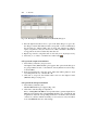
When Lahey Fortran compiler is used:
– Create a transparent file by specifying FORM = ’UNFORMATTED’ and ACCESS = ’TRANSPARENT’ in the OPEN statement.
When Intel Visual Fortran is used:
– Create a transparent file, if it is opened using FORM = ’BINARY’ and ACCESS = ’SEQUENTIAL’.
If you are using other compilers, please consult the user manual for the settings
of creating ”transparent” binary files.
2
Modeling Environment
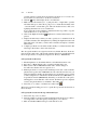
This chapter is a complete reference of the user interface of PM.
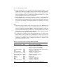
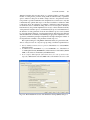
With the exception of PHT3D, PM requires the use of consistent units throughout
the modeling process. For example, if you are using length [L] units of meters and
time [T ] units of seconds, hydraulic conductivity will be expressed in units of [m/s],
pumping rates will be in units of [m3 /s] and dispersivity will be in units of [m]. The
values of the simulation results are also expressed in the same units. Table 2.1 lists
symbols and their units, which are used in various parts of this text.
PHT3D requires the use of meters for the length, the use of mol/lw for concentrations of aqueous (mobile) chemicals and user-defined immobile entities such
as bacteria and the use of mol/lv for mineral, exchanger and surface concentrations,
where mol refers to moles, lw refers to liter of pore water and lv refers to liter of bulk
volume (see Prommer and others [97] for details about the use of units in PHT3D).
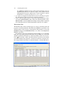
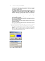
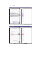
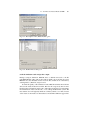
PM contains the following menus File, Grid, Parameters, Models, Tools, Value,
Options, and Help. The Value and Options menus are available only in the Grid
Editor and Data Editor (see Sections 2.1 and 2.2 for details). PM uses an intelligent
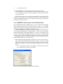
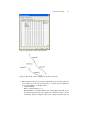
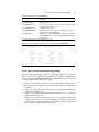
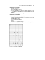
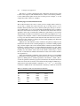
Table 2.1 Symbols used in the present text
Symbol
Meaning
Unit
m
HK
VK
T
Ss
S
Sy
ne
V CON T
HAN I
thickness of a model layer
horizontal hydraulic conductivity along model rows
vertical hydraulic conductivity
transmissivity; T = HK × m
specific storage
storage coefficient or storativity; S = Ss × m
specific yield or drainable porosity
effective porosity
vertical leakance
horizontal anisotropy
HAN I × HK = horizontal hydraulic conductivity along columns
vertical anisotropy; HK = V K × V AN I
[L]
[LT −1 ]
[LT −1 ]
[L2 T −1 ]
[L−1 ]
[−]
[−]
[−]
[T −1 ]
[−]
V AN I
[−]
8
2 Modeling Environment
Table 2.2 Summary of menus in PM
Menu
Description
File
Create new models; open existing models; convert models to the PM format;
Save and print plots.
Generate or modify the size of a model grid; input of the geometry of the
aquifer.
Input of spatial aquifer parameters, for example transmissivity; Input of temporal parameters, for example simulation length or number of stress periods.
Specify model-specific data using the module provided and call simulation
programs. For example, the user can add wells, use the recharge or river
modules to MODFLOW or define the advection or dispersion parameters in
MT3DMS. The simulation programs are called by selecting Run from the
corresponding model.
Call the modeling tools.
Manipulate model data; read or save model data in separate files; import
model results; import an existing MODFLOW input file.
Modify the appearance of the model grid on the screen; load site maps;
change display mode; change input method.
Call Processing Modflow Pro Help.
Grid
Parameters
Models
Tools
Value
Options
Help
menu system to help you control the modeling process. If a model data set has been
specified, the corresponding item of the Grid, Parameters, and Models menus will be
checked. To deactivate a selected item in the Models menu, just select the item again.
If the user does not know which model data still needs to be specified, one may try to
run the model by selecting the menu item Run from the corresponding model in the
Models menu. PM will check the model data prior to running the model. A summary
of the menus in PM is given in Table 2.2.
A toolbar with buttons representing PM operations or commands is displayed
below the menus. The toolbar is a shortcut for the pull-down menus. To execute one
of these shortcuts, move the mouse pointer over the toolbar button and click on it.
Most of the user-specified data is saved in binary files. Prior to running the supported models or the parameter estimation programs, PM will generate the required
ASCII input files. The names of the ASCII input files are given in Section 6.3. The
formats of the input files of can be found in the user’s guides of the corresponding
model. The particle-tracking model PMPATH retrieves the binary data files of PM
directly, thus no ASCII input file is required by PMPATH.
2.1 The Grid Editor
The first steps in the groundwater modeling process are to define the goals of the
model, select a computer code, collect the necessary data, develop a conceptual
model of the groundwater system and define the spatial discretization of the model
domain. Anderson and Woessner [8] discuss the steps in going from aquifer systems to a numerical model grid. Zheng and Bennett [118] describe the design of
2.1 The Grid Editor
9
model grids, which are intended for use both in flow and transport simulations. These
sources provide valuable general information relating to spatial discretization and
grid design in numerical groundwater modeling.
In the block-centered finite difference method, an aquifer system is replaced by
a discretized domain consisting of an array of nodes and associated finite difference
blocks (cells). Fig. 2.1 shows the spatial discretization scheme of an aquifer system
with a mesh of cells and nodes at which hydraulic heads are calculated. The nodal
grid forms the framework of the numerical model. Hydrostratigraphic units can be
represented by one or more model layers. The thickness of each model cell and the
width of each column and row can be specified. The locations of cells are described in
terms of layers, rows, and columns. PM uses an index notation [Layer, Row, Column]
for locating the cells. For example, the cell located in the first layer, 6th row, and 2nd
column is denoted by [1, 6, 2]. To generate or modify a model grid, select Grid |
Fig. 2.1. Spatial discretization of an aquifer system and the cell incides
Mesh Size. If a grid does not exist, a Model Dimension dialog box (Fig. 2.2) appears
for specifying the extent and number of layers, rows, and columns of the model grid.
After specifying these data and clicking the OK button, the Grid Editor shows the
model grid (Fig. 2.3). A summary of the tool bar buttons of the Grid Editor is given
in Table 2.3. Using the Environment Options dialog box (see Section 2.9.2), the user
can adjust the coordinate system, the extent of the Viewing Window and the position
of the model grid to fit the study site. By default, the origin of the coordinate system
is set at the lower-left corner of the model grid and the extent of the Viewing Window
is set to twice that of the model grid. The first time the Grid Editor is used, the user
10
2 Modeling Environment
Fig. 2.2. The Model Dimension dialog box
can insert or delete columns or rows (see below). After leaving the Grid Editor and
saving the grid, the existing model grid can be subsequently refined by calling the
Grid Editor again. In each case, the width of any column or row can be modified. If
the grid is refined, depending on the nature of the model parameters, they are either
kept the same or scaled by the cell size. The following rules apply:
1. Pumping rates, mass-loading rate (see Section 2.6.2.9) and cell-by-cell conductance values of the river, drain, general-head boundary, and stream are scaled
by the cell volume. For example, if a well cell is refined to four cells, all four
refined cells will be treated as wells, each with 1/4 of the original pumping rate.
The sum of their pumping rates remain the same as that of the previous single
well.
2. The parameters of polylines, which are used to define river, drain, general-head
boundary, or stream, remain the same, since they are grid-independent. If a
stream (of the Stream-Routing package) is defined by using cell-by-cell values,
you must redefine the segment and reach number of the stream.
3. Transmissivity (T) and storage coefficient (S) values are scaled by the thickness.
4. All other model parameters remain the same.
I To change the width of a column and/or a row
1. Click the assign value button .
The grid cursor appears only if the Assign Value button is pressed down. You do
not need to click this button, if it is already depressed.
2.1 The Grid Editor
11
Fig. 2.3. The Grid Editor
2. Move the grid cursor to the desired cell by using the arrow keys or by clicking
the mouse on the desired position. The sizes of the current column and row are
shown on the status bar.
3. Press the right mouse button once. The Grid Editor shows the Grid Size dialog
box (Fig. 2.4).
4. In the dialog box, type new values, then click OK.
I To insert or delete a column and/or a row
1. Inserting or deleting columns/rows is only possible when using the Grid Editor
for the first time. Click the assign value button .
2. Move the grid cursor to the desired cell by using the arrow keys or by clicking
the mouse on the desired position.
3. Hold down the Ctrl-key and press the up or right arrow keys to insert a row or a
column; press the down or left arrow keys to delete the current row or column.
12
2 Modeling Environment
Table 2.3 Summary of the toolbar buttons of the Grid Editor
Button
Name
Action
Leave editor
Leave the Grid Editor and return to the main menu of PM.
Assign value
Allows the user to move the grid cursor and change the widths
of grid columns and rows.
Pan
Moves the Viewing Window up, down, or sideways to display
areas of the model domain which, at the current viewing scale, lie
outside the Viewing Window. By dragging the mouse, the model
grid and sitemaps will be moved in the same direction as the
mouse cursor. When the left mouse button is released, the grid
and maps will be redrawn.
Zoom in
Allows the user to zoom-in by dragging a window over a part of
the model domain.
Zoom out
Display the entire worksheet.
Rotate grid
To rotate the model grid, point the mouse pointer to the grid, left
click and hold down the mouse button, and move the mouse.
Shift grid
Allows the user to move the model grid to another position. To
shift the model grid, point the mouse pointer to the grid, left click
and hold down the mouse button, and move the mouse.
Map View
Switch to the Map View display mode.
Column View
Switch to the column cross-sectional display mode.
Row View
Switch to the row cross-sectional display mode.
Duplication
on/off
If duplication is turned on, the size of the current row or column
will be copied to all rows or columns passed by the grid cursor.
Duplication is on, when this button is depressed.
I To refine a layer, a row or a column
1. Refining a grid is only possible when the grid has already been saved. Click the
assign value button .
2. Move the grid cursor to the desired cell by using the arrow keys or by clicking
the mouse on the desired position.
3. Press the right mouse button once. The Grid Editor shows the Grid Size dialog
box (Fig. 2.4).
4. In the dialog box, type new values, then click OK.
2.2 The Data Editor
13
Fig. 2.4. The Grid Size dialog box
2.2 The Data Editor
The Data Editor is used to assign parameter values to the model. To start the Data
Editor, select a corresponding item from the Grid, Parameters or Models menus. For
example, select Parameters | Porosity to assign porosity values to the model.
The Data Editor provides four display modes - Map View, Grid View, Column
View, and Row View. It has three methods for specifying parameter values - Cellby-cell, Polygon, and Polyline methods. The input methods are discussed in sections
2.2.1, 2.2.2, and 2.2.3. The Polyline method is available only for specifying data to
the River, Drain, General-head boundary and Streamflow-Routing packages.
In the Grid View display mode, the Viewing Window is aligned with the model
grid (Fig. 2.5). In the Map View display mode, the Viewing Window is aligned with
the orthogonal Northing and Easting coordinate axes. A rotated model grid is displayed on the Map View similar to Fig. 2.6. In the Row or Column (cross-sectional)
View, the Viewing Window is aligned with the vertical axis (Fig. 2.7).
Using the Environment Options dialog box (see Section 2.9.2) the user can adjust
the vertical exaggeration factor for the cross-sectional display, the coordinate system,
the horizontal extent of the Viewing Window, and the position of the model grid to fit
the condition of the study area. Regardless of the display modes, the mouse pointer
position [x, y, z] is always expressed in the world coordinates according to the userdefined coordinate system, and [K, I, J] is expressed in [Layer, Row, Column] cell
indices. The position of the grid cursor is shown in the tool bar. The grid cursor can
be moved by using the arrow keys, clicking the mouse on the desired position, using
buttons in the tool bar, or typing the new position in the layer/row/column edit
fields and pressing the Enter key. The parameter values of the cell pointed to by the
grid cursor are displayed from left to right in the status bar. A summary of the tool
bar buttons of the Data Editor is given in Table 2.4.
14
2 Modeling Environment
Fig. 2.5. The Data Editor (Grid View)
Fig. 2.6. The Data Editor (Map View)
2.2 The Data Editor
15
Table 2.4 Summary of the toolbar buttons of the Data Editor
Button
Name
Action
Leave editor
Leave the Data Editor and return to the main menu.
Assign value
Allow the user to move the grid cursor and assign values to
model cells.
Pan
Moves the Viewing Window up, down, or sideways to display
areas of the model domain which, at the current viewing scale,
lie outside the Viewing Window. By dragging the mouse, the
model grid and sitemaps will be moved in the same direction
as the mouse cursor. When the left mouse button is released,
the grid and maps will be redrawn.
Zoom in
Allow the user to drag a zoom-window over a part of the model
domain.
Zoom out
Display the entire worksheet.
Cell-by-cell input method
Switch to the Cell-by-cell input method.
Polygon
method
input
Switch to the Zone input method.
Polyline
method
input
Switch to the Polyline input method.
Grid view
Switch to the Grid View display mode.
Map view
Switch to the Map View display mode.
Column View
Switch to the column cross-sectional display mode.
Row View
Switch to the row cross-sectional display mode.
Duplication
on/off
If duplication is turned on, the size of the current row or column will be copied to all rows or columns passed by the grid
cursor. Duplication is on, when this button is depressed.
Layer,
Column
on/off
Row,
Copy
When this button is depressed, Layer/row/column copy is on
and the following rules apply: (1) If the display mode is Grid
View or Map View, when moving to another layer the zones
and cell values of the current layer will be copied to the destination layer; (2) If the display mode is Row View, when moving to another column the cell values of the current row crosssection will be copied to the destination row cross-section; (3)
If the display mode is Column View, when moving to another
column the cell values of the current column cross-section will
be copied to the destination column cross-section.
Change
period
stress
Manage model data for transient simulations.
16
2 Modeling Environment
Fig. 2.7. The Data Editor (Cross-sectional View)
2.2.1 The Cell-by-Cell Input Method
To activate this method, click the
By-Cell.
button or select Options | Input Method | Cell-
I To assign new value(s) to a cell
1. Click the assign value button .
It is not necessary to click this button, if the button is already depressed.
2. Move the grid cursor to the desired cell by using the arrow keys or by clicking
the mouse on the cell. The value(s) of the current cell is (are) displayed in the
status bar.
3. Press the Enter key or press the right mouse button once.
The Data Editor shows a dialog box.
4. In the dialog box, type new value(s) then click OK.
Since groundwater model data are often very complex, PM provides several possibilities for checking or modifying cell-by-cell model data as listed below.
•
Double-click a cell.
All model cells with the same value will appear in the same color. The color can
be changed by repeated double-clicks.
2.2 The Data Editor
17
Fig. 2.8. The Cell Information dialog box
Fig. 2.9. The Search and Modify Cell Values dialog box
•
•
•
Shift + left mouse button or Ctrl+Q.
Open the Cell Information dialog box (Fig. 2.8), which displays the user-specified
data of the cell pointed to by the grid cursor.
Ctrl + left mouse button. Open the Search and Modify Cell Values dialog box
(Fig. 2.9). This allows you to display all cells that have a value located within
the Search Range (to be specified). According to the user specified Value and the
operation Options, you can easily modify the cell values. For example, if Add
is used, the user-specified value will be added to the cell value. The Parameter
drop-down box shows the available parameter type(s). The user may select the
parameter to which the subsequent Search and Modify operation will be applied.
Select Value | Search and Modify or press Ctrl+S.
Open a Search and Modify dialog box for more advanced data manipulation features. See Section 2.8.5 for details.
2.2.2 The Polygon Input Method
The Polygon Input Method allows the user to assign parameter values to model cells
with the help of polygons. This input method is not allowed in the cross-sectional
view. To activate this method, click on the
button or the
button to switch to
Grid View or Map View, and then click on the
button or choose Options | Input
18
2 Modeling Environment
Method | Polygon. The use of this input method is straightforward. First, you draw
a polygon and then assign parameter values to the polygon. Finally, press the
button to apply the parameter values to model cells that lie within the polygon.
Note. Polygon data is not used by PM for model computation directly. If polygon data is not applied to the model cells, the original values in the cells are used.
I To draw a polygon
button or the
1. If the display mode is not Grid View or Map View, click the
button to switch to the Grid View or Map View.
2. Click the assign value button
and click the
button.
3. Click the mouse pointer on a desired position to anchor one end of a line.
4. Move the mouse pointer to another position then press the left mouse button
again.
5. Repeat steps 3 and 4 until the polygon is closed or press the right mouse button
to abort.
I To delete a polygon
1. If the display mode is not Grid View or Map View, click the
button to switch to the Grid View or Map View.
and click the
button.
2. Click the assign value button
3. Move the mouse pointer into a polygon.
The boundary of the polygon will be highlighted.
4. Press the Delete key.
button or the
I To assign value(s) to polygons
1. If the display mode is not Grid View or Map View, click the
button or the
button to switch to the Grid View or Map View.
2. Click the assign value button
and click the
button.
3. Move the mouse pointer into a polygon.
The boundary of the polygon will be highlighted. The value(s) of the polygon
will be displayed in the status bar.
4. Press the right mouse button once.
The Data Editor displays a dialog box, which allows the user to assign parameter
value(s) to the polygon.
5. In the dialog box, type new parameter value(s) then click the
button to apply
the parameter value(s) to the model cells within the polygon.
2.2 The Data Editor
19
I To modify a polygon
1. The user may drag vertices of a polygon by pointing the mouse pointer at a
vertex node and pressing down the left mouse button while moving the mouse.
2. If there are several polygons, some polygons can intersect or even cover other
polygons. If the mouse pointer is moved into a covered polygon, the boundary of
the polygon will not be highlighted. In this case, simply move the mouse pointer
into that polygon, hold down the Ctrl key and press the left mouse button once.
The Data Editor will resort the order of the polygons and the ”lost” polygon will
be recovered.
2.2.3 The Polyline Input Method
The Polyline Input Method is available only for the Drain, General-head boundary,
River and Streamflow-Routing packages. This input method is not allowed in the
button or the
butcross-sectional view. To activate this method, click on the
button or choose
ton to switch to Grid View or Map View, and then click on the
Options | Input Method | Polyline. The use of this input method is straightforward.
First, you draw a polyline along a drain, river, or stream, and then assign parameter
values to vertices of the polyline. Within a polyline, parameter values needed for
constructing MODFLOW input files are assigned to at least one vertex. Properties
needed for cells along traces of polylines are obtained using the parameter values
of vertices. These property values are used in addition to the cell-by-cell values to
generate MODFLOW input files prior to running MODFLOW.
I To draw a polyline
1. If the display mode is not Grid View or Map View, click the
button or the
button to switch to the Grid View or Map View.
2. Click the assign value button
and click the
button.
3. Click the mouse pointer on a desired position to anchor one end of a line.
4. Move the mouse pointer to another position then press the left mouse button
again.
5. Repeat steps 3 and 4 until the desired polyline is drawn, click on the latest vertex
again to complete the polyline or press the right mouse button to abort drawing.
I To delete a polyline
button or the
1. If the display mode is not Grid View or Map View, click the
button to switch to the Grid View or Map View.
2. Click the assign value button .
3. Move the mouse pointer over a polyline. The polyline will be highlighted.
4. Press the Delete key.
20
2 Modeling Environment
Follow the steps below to assign parameter values to polylines. Refer to the explanation of the River, Drain, General-head boundary, and Streamflow-routing packages
for details about the required parameters of each package.
I To assign value(s) to polylines
button or the
1. If the display mode is not Grid View or Map View, click the
button to switch to the Grid View or Map View.
2. Click the assign value button
and click the
button.
3. Move the mouse pointer over a vertex and right-click.
The Data Editor displays a dialog box, which allows the user to assign parameter
value(s) to the vertex.
4. In the dialog box, type new parameter value(s).
Once the parameter values are specified, the display color of the vertex is
changed to indicate that its parameter values are specified.
I To modify a polyline
1. The user may drag vertices of a polyline by pointing the mouse pointer at a
vertex node, pressing down the left mouse button, and moving the mouse.
2. Use Shift+left click on a segment of the polyline to insert a new vertex.
3. Use ctrl+left click on a vertex to delete it.
2.2.4 Specifying Data for Transient Simulations
button appears in the Tool bar.
If a model has more than one stress period, the
Clicking on this button opens the Temporal Data dialog box (Fig. 2.10), which is
used to manage model data for transient simulations. The following describes the
use of the dialog box.
•
The table displays the status of the model data of each stress period. The boxes
in the Data Status column have three states:
–
: Model data has been specified and will be used for the simulation.
–
: Model data has been specified, but will not be used. The model data from
the previous stress period will be used for the simulation.
–
: Model data has not been specified. The model data from the previous
stress period will be used for the simulation.
Click on the Data boxes to toggle between and . Fig. 2.10 shows an example
in which the model data for the periods 1, 3, 4 are specified. The specified data
of the first period will be used throughout the first three periods. The data of the
fourth period will be used for the rest of the simulation. The model data of the
third period has been specified, but will not be used for the simulation since the
Data Status is .
2.3 The File Menu
21
Fig. 2.10. The Temporal Data dialog box
•
•
Edit Data: To edit model data for a particular stress period, select a row of the
table and click the Edit Data button. After having specified the model data of a
stress period, the Data status changes to .
Copy Data: To copy model data from one stress period to another.
2.3 The File Menu
2.3.1 New Model
Select New Model to create a new model. A New Model dialog box allows the user
to specify a filename on any available folder or drive for the new model. A PM
model must always have the file extension .pm5, which has been kept consistent since
PMWIN version 5. All file names valid under the MS Windows operating system
with up to 120 characters can be used. It is a good idea to save every model in a
separate folder, where the model and its output data will be kept. This will also allow
the user to run several models simultaneously (multitasking).
2.3.2 Open Model
Use Open Model to load an existing PM model. Once a model is opened, PM displays the filename of the model on the title bar.
2.3.3 Convert Model
A Convert Models dialog box appears after selecting this menu item. The options
in this dialog box are grouped under 4 tabs - PMWIN 4.x, MODFLOW-88/96,
22
2 Modeling Environment
Fig. 2.11. The Convert Model dialog box
MODFLOW-2000/2005, and Telescoping Flow Model (Fig. 2.11). The tabs are described below. In addition, the user can specify refinement factors for both column
and row directions. In this way, one can load or create a model with a higher resolution for transport simulations.
•
•
•
•
PMWIN 4.x tab: This tab is used to convert groundwater models created by
PMWIN 4.x to PM. To convert, click the open file button
and select a
PMWIN 4.x model from an Open dialog box, then click the Convert button to
start the conversion. Groundwater models created by PMWIN 5.x or later are
compatible with PM and do not need to be converted.
MODFLOW-88/96 tab: This tab is used to import models stored in MODFLOW88 or MODFLOW-96 formats to PM. To import, click the open file button
and select a MODFLOW Name File from an Open dialog box, then click the
Convert button to start the conversion. Refer to Section 6.3.1 for the definition of
the name file. A MODFLOW-88/96 name file usually has lines with the file type
(i.e., Ftype) ”BAS” or ”BCF”.
MODFLOW-2000/2005 tab: This tab is used to import models stored in MODFLOWand select a
2000/2005 formats to PM. To import, click the open file button
MODFLOW Name File from an Open dialog box, then click the Convert button
to start the conversion. Refer to Section 6.3.1 for the definition of the name file. A
MODFLOW-2000/2005 name file usually has lines with the file type (i.e., Ftype)
”BAS6”, ”BCF6”, or ”LPF”.
Telescoping Flow Model (Fig. 2.12): This tab creates local-scale sub-models
from a regional scale model. To create a sub-model, select an existing PM model
and specify the sub-region. Then click the Convert button. Prior to converting, the
flow simulation of existing PM model must be performed. The sub-region is defined by the starting and ending columns and rows. PM automatically transfers
the model parameters and the calculated heads from the regional model to the
sub-model. The boundary of the sub-model will be set to constant head boundary (for steady-state simulations) or time-variant specified-head boundary (for
transient simulations).
2.3 The File Menu
23
Fig. 2.12. Telescoping a flow model using the Convert Model dialog box
2.3.4 Preferences
The Preferences dialog box (Fig. 2.13) defines the MODFLOW version and manages
the paths to the simulation programs of an opened PM model. The settings of the
dialog box are described below.
Fig. 2.13. The Preferences dialog box
•
Modflow Version: Several variants of MODFLOW are supported and included
in PM. Each variant is associated with an executable program. The full paths
and file names of all executable programs of MODFLOW are given in Table 2.5.
The default Modflow Version is ”MODFLOW-96”. This version works with all
supported transport models. Of particular note is that when using MODFLOW2000 for parameter estimation, Modflow Version must be set to ”MODFLOW2000/MODFLOW-2005”, otherwise it is not possible to switch the Flow Package (see below) to the LPF package, which are required for estimating aquifer
parameters within MODFLOW-2000.
24
•
2 Modeling Environment
Flow Package: This dropdown box is enabled, when Modflow Version is set to
MODFLOW-2000/MODFLOW-2005, which includes the Layer-Property Flow
(LPF) and the Block-Centered Flow (BCF) packages for formulating inter-cell
hydraulic conductance terms. As the BCF or LPF packages require different
aquifer parameters for formulating finite difference equations of groundwater
flow, it is important to notice the following major differences between these two
packages:
– The Block Centered Flow (BCF) package supports four layer types. Depend
on the selected layer type; the required aquifer parameters of a model layer
are different and listed below. Layer type 0: T and S
Layer type 1: HK and Sy.
Layer type 2: T, S and Sy.
Layer type 3: HK, Sy and S.
Note that S and Sy are required only for a transient flow simulation. All layer
types use VCONT to describe the vertical conductance between two layers.
– The Layer-Property Flow package has only two layer types - confined and
convertible (i.e., convertible between confined and unconfined). Independent
of the selected layer type; a model layer always requires HK, Ss, and VK or
VANI. The only exception is Sy, which is required only if the layer is convertible (note that Ss and Sy are required only for a transient flow simulation).
When the Layer-Property Flow package is selected, the menu items Transmissivity, Vertical Leakance and Storage Coefficient of the Parameters menu
are dimmed and cannot be used (don’t need to be used).
Note.
– All versions of Modflow and either BCF or LFP package can be used with
PEST for estimating parameters. However, one can only estimate the required
aquifer parameters of the BCF or LPF package as given above.
– As the BCF package does the not support the required parameterization
method of MODFLOW-2000, this package cannot be used with the builtin model calibration capability of MODFLOW-2000. That is, the user cannot
estimate aquifer parameters when using BCF with MODFLOW-2000.
– The settings of Modflow Version and Flow Package are saved with the model,
i.e., if the model is used on another computer these settings will remain the
same.
Table 2.5 Versions and Filenames of MODFLOW
Version
Filename
MODFLOW-96 pmdir\modflw96\lkmt2\modflow2i.exe
MODFLOW-2000 pmdir\mf2k\mf2ki.exe
MODFLOW-2005 pmdir\modflow2005\mf2005.exe
– pmdir is the folder in which PM is installed, for example C:\Simcore\PM8.
2.3 The File Menu
•
25
Module/Models: The supported modules or models are listed below. Each module/model is associated with a program. Note that some modules are optional and
may not appear on the user’s computer.
– MODFLOW is groundwater flow simulation program, which is used when
selecting the menu item Modflow | Run.
– PMPATH is a particle-tracking model (also referred to as advective transport)
included in PM.
– Text Viewer, which can be any text editors, is used to display simulation result
files, which are saved in ASCII.
– MODFLOW-2000 (Parameter Estimation): The associated program is used
when selecting the menu item MODFLOW-2000 (Parameter Estimation) |
Run | MODFLOW-2000.
– PEST (Parameter Estimation): PEST [33][34] is a program for parameter estimation. The associated program is used when selecting the menu item PEST
(Parameter Estimation) | Run or MODFLOW-2000 (Parameter Estimation) |
Run | PEST-ASP+MODFLOW-2000. Note that the latter requires PEST-ASP
and a special version of MODFLOW-2000, called MF2K-ASP, which are automatically installed.
– MT3D: MT3D is a single-species solute transport model, which has been prepared by Zheng [117][120] and has been improved subsequently over years.
The associated program is used when selecting the menu item MT3D | Run.
– MOC3D: MOC3D [74] is a single-species solute transport model using the
method of characteristics. The associated program is used when selecting the
menu item MOC3D | Run.
– MT3DMS: MT3DMS [121][123] is a multi-species solute transport model.
The associated program is used when selecting the menu item MT3DMS/SEAWAT
| Run. If the user intends to use MT3D99 [122], the MT3D99 program should
be assigned to this module, and the MT3D99 and MODFLOW programs
must be compiled with the same compiler.
– 3D Visualization: The software Seer3D [] is available separately. When installed, Seer3D can be started by selecting the menu item Tools | 3D Visualization.
– RT3D: The RT3D model [25][26][27]) simulates reactive-flow and transport
of multiple mobile and/or immobile species. The PM installation includes
three versions of RT3D - rt3d1v.exe (version 1), rt3d2v.exe (version 2), and
rt3d25v.exe (version 2.5). They can be found in the folder \pmhome\rt3d,
where pmhome is the installation directory of PM. The associated program
is used when selecting the menu item RT3D | Run.
– PHT3D: PHT3D [97] couples MT3DMS [123] for the simulation of threedimensional advective-dispersive multi-component transport and the geochemical model PHREEQC-2 [91] for the quantification of reactive processes. The associated program is used when selecting the menu item PHT3D
| Run.
26
2 Modeling Environment
–
•
•
SEAWAT: SEAWAT is designed to simulate three-dimensional, variabledensity, saturated groundwater flow and transport. The associated program
is used when selecting the menu item MT3DMS/SEAWAT | Run.
Active: Check or clear the active flag to activate or deactivate a model/module.
Please note that the first three modules MODFLOW, PMPATH and TEXT
VIEWER are required and cannot be deactivated. When a module is deactivated,
its associated menu item under the Models menu is removed. This feature is useful, when several modules are not used and the Models menu should be kept as
short as possible. Deactivating or activating of a module does not affect the model
data in any way.
Paths to Simulation Program File: If the user intends to use an executable program located in another position, click the corresponding button and select the
desired program from a dialog box.
Note. The following programs must be located in the same directory as the PEST
(PEST-ASP) program: mf2kasp.exe, mf2pest.exe, modbore.exe, par2sen.exe, and
pestchek.exe.
2.3.5 Save Plot As
Use Save Plot As to save the contents of the worksheet in graphics files. Three graphics formats are available: Drawing Interchange File (DXF), Hewlett-Packard Graphics Language (HP-GL) and Windows Bitmap (BMP). DXF is a fairly standard format
developed by Autodesk for exchanging data between CAD systems. HP-GL is a twoletter mnemonic graphics language developed by Hewlett-Packard. Most graphics or
word-processing software, and graphics devices can process these graphics formats.
To save a plot, use the Format drop-down box to select a graphic format. Then, enand select a file from a dialog
ter a filename into the File edit field, or click
box. When finished, click OK. Note that in the Map View display mode only the
BMP-format may be used.
2.3.6 Print Plot
This menu item is only activated in the Data Editor. After selecting this item, a Print
Plot dialog box is displayed with a preview window. The options are described below.
•
•
•
•
•
Use full page: The plot is scaled to fit the paper; the original aspect ratio will not
be changed.
Center on page: The plot is placed on the center of the page.
Image Size (millimeters): Specify the width and height of the printed image in
millimeters.
Margins (millimeters): Specify the left and top margins of the image in millimeters.
Printer: A Printer dialog box allows the user to select an installed printer and
specify the print quality, the paper size, source and orientation and other printing
parameters.
2.4 The Grid Menu
•
•
27
Print: Print the contents shown on the preview window.
Close: Close the Print Plot dialog box without printing.
2.3.7 Animation
This menu item is only activated when the 2D Visualization (Tools | 2D Visualization) tool is selected. Before creating an animation sequence, the user should use the
Environment Option and Maps Option dialog boxes (refer to Section 2.9 for details)
to make sure that the model grid, maps and contours are set properly.
I To create an animation sequence
1. Select File | Animation to display an Animation dialog box.
to display a Save File
2. In the Animation dialog box, click the open file button
dialog box.
Select an existing frame file or specify a new base file name for the frame files in
the dialog box, then click Open. Like a movie, an animation sequence is based on
a series of of frames. Each frame is saved by using the filename basename.nnn,
where basename is the base file name and nnn is the serial number of the frame
files.
Note. To protect the model data, the frame files must not be saved in the same
folder as the model data.
3. Check or clear Create New Frames.
Check Create New Frames if a new animation sequence should be created. Clear
the Create New Frame box if a saved sequence should be played back.
4. Set Delay(s). Delay is the number of seconds between frames.
5. In the Animation dialog box, click OK to start the animation. PM will create
a frame (image) for each time point at which the simulation results have been
saved. When all frames are created, PM will repeat the animation indefinitely
until the Esc key is pressed.
2.4 The Grid Menu
2.4.1 Mesh Size
Allows the user to generate or modify a model grid using the Grid Editor. See Section
2.1 for how to use the Grid Editor.
2.4.2 Layer Property
The layer properties are defined in the Layer Property dialog box (Fig. 2.14). Many
settings of this dialog box depend on the selection between the Block-CenteredFlow (BCF) and Layer Property Flow (LPF) packages. Refer to Section 2.3.4 for
details about the BCF and LPF package. When the LPF Package is used, the columns
28
2 Modeling Environment
Transmissivity, Leakance and Storage Coefficient are dimmed to indicate that their
settings are ignored, because the LPF package only uses HK, VK, Ss and Sy. When
the BCF package is used, the column Vertical Anisotropy is dimmed since it is not
supported by the BCF package. The settings of this dialog box are described below.
•
Type: The numerical formulations, which are used by the BCF or LPF package to
describe groundwater flow, depend on the type of each model layer. The available
layer types are:
– Type 0: The layer is strictly confined. For transient simulations, the confined
storage coefficient (specific storage × layer thickness) is used to calculate the
rate of change in storage. Transmissivity of each cell is constant throughout
the simulation.
– Type 1: The layer is strictly unconfined. The option is valid for the first layer
only. Specific yield is used to calculate the rate of change in storage for this
layer type. During a flow simulation, transmissivity of each cell varies with
the saturated thickness of the aquifer.
– Type 2: A layer of this type is partially convertible between confined and
unconfined. Confined storage coefficient (specific storage × layer thickness)
is used to calculate the rate of change in storage, if the layer is fully saturated,
otherwise specific yield will be used. Transmissivity of each cell is constant
throughout the simulation. Vertical leakage from above is limited if the layer
desaturates.
– Type 3: A layer of this type is fully convertible between confined and unconfined. Confined storage coefficient (specific storage × layer thickness) is used
to calculate the rate of change in storage, if the layer is fully saturated, otherwise specific yield will be used. During a flow simulation, transmissivity of
each cell varies with the saturated thickness of the aquifer. Vertical leakage
from above is limited if the layer desaturates.
Fig. 2.14. The Layer Property dialog box
2.4 The Grid Menu
•
•
•
•
29
Note that the LPF package uses only two layer types - confined and convertible.
Layer type 0 will be interpreted by the LPF package as confined and all other
layer types will be interpreted as convertible layers, i.e. the layers are convertible
between confined and unconfined.
Horizontal Anisotropy: The ratio of the horizontal hydraulic conductivity along
columns to hydraulic conductivity along rows. The latter is specified by selecting
Parameters | Horizontal Hydraulic Conductivity.
– When the LPF package is used, a positive Horizontal Anisotropy value indicates that horizontal anisotropy is constant for all cells in the layer and the
anisotropy is the specified value. A negative value indicates that horizontal
anisotropy can vary at each cell in the layer. The cell-by-cell anisotropy values are specified by selecting Parameters | Horizontal Anisotropy.
– When the BCF package is used, horizontal anisotropy is constant for all cells
in the layer and the anisotropy is the absolute value of the specified Horizontal
Anisotropy value.
Vertical Anisotropy: The setting of this column is either VK or VANI.
– VK indicates that vertical hydraulic conductivity is used for the layer and is
to be specified by selecting Parameters | Vertical Hydraulic Conductivity.
– VANI indicates that vertical anisotropy is used for the layer and is to be specified by selecting Parameters | Vertical Anisotropy.
Transmissivity: MODFLOW (or exactly to say, the BCF package) requires transmissivity (= horizontal hydraulic conductivity [LT −1 ] × layer thickness [L]) for
layers of type 0 or 2. PM provides two options for each model layer to facilitate
the data input:
– Set the Transmissivity setting of a layer to User-Specified:
The user-specified transmissivity values of the layer are used in the simulation.
– Set the Transmissivity setting of a layer to Calculated:
PM calculates transmissivity of the layer by using user-specified horizontal
hydraulic conductivity and the elevations of the top and bottom of the layer.
The calculated transmissivity values are used in the simulation.
Leakance: For flow simulations involving more than one model layer, MODFLOW (BCF package) requires the input of the vertical conductance term, known
as vertical leakance (VCONT array), between two model layers. MODFLOW
uses VCONT to formulate the flow rate equation between two vertically adjacent
cells. PM provides two options for each model layer to facilitate the data input:
– Set the Leakance setting of a layer to User-Specified:
The user-specified vertical leakance values are used in the simulation. In the
Data Editor, the vertical leakance between the layers i and i+1 is given as the
data of the i-th layer. The leakance data are not required for the bottom layer
since MODFLOW assumes that the bottom layer is underlain by impermeable material.
– Set the Leakance setting of a layer to Calculated:
PM calculates vertical leakance by using the rules explained below. The calculated vertical leakance values are used in the simulation.
30
2 Modeling Environment
As illustrated in Fig. 2.15a, when each model layer represents a different
hydrostratigraphic unit or when two or more layers represent a single hydrostratigraphic unit, PM uses equation 2.1 to calculate the vertical leakance
VCONT.
V CON T =
2
∆νk
∆νk+1
+
(Kz )k,i,j
(Kz )k+1,i,j
(2.1)
where (Kz )k,i,j and (Kz )k+1,i,j are the vertical hydraulic conductivity values of layers k and k+1, respectively. The ratio of horizontal to vertical hydraulic conductivity ranging from 1:1 to 1000:1 is common in model application [8]. A summary of hydraulic conductivity values can be found in [109].
It is not uncommon to represent resistance to flow in a low hydraulic conductivity unit (2.15b, semiconfining unit) by lumping the vertical hydraulic
conductivity and thickness of the confining unit into a vertical leakance term
between two adjacent layers. These kinds of models are often called quasi
three-dimensional models, because semi-confining units are not explicitly
included in a simulation. In this case the user must manually calculate the
VCONT values using equation 2.2 and enter them into the Data Editor.
V CON T =
2
∆νu
∆νc
∆νL
+
+
(Kz )u
(Kz )c
(Kz )L
(2.2)
where (Kz )u , (Kz )c , and (Kz )L are the vertical hydraulic conductivity values of the upper layer, semi-confining unit and lower layer, respectively.
Fig. 2.15. Grid configuration used for the calculation of VCONT
•
Storage Coefficient: For transient flow simulations, MODFLOW (BCF package)
requires dimensionless storage terms to be specified for each model layer. For a
confined layer, these storage terms are given by the confined storage coefficient
(=specific storage [L−1 ] × layer thickness [L]). If the Storage Coefficient setting
2.4 The Grid Menu
•
31
is set to Calculated, PM uses user-specified specific storage and the elevations of
the top and bottom of each layer to calculate the confined storage coefficient. Set
the Storage Coefficient flag to User Specified, if you want to specify the confined
storage coefficient manually. For an unconfined layer, the storage values are equal
to specific yield [−]. The setting of the Storage Coefficient flag has no influence
on the specific yield.
Interbed Storage: PM supports the Interbed-Storage package for calculating storage changes from both elastic and inelastic compaction of each model layer.
Check the Interbed Storage setting of a specific layer to calculate its storage
changes and compaction by using the Interbed-Storage package. Refer to Section 2.6.1.5 for details about this package.
2.4.3 Cell Status
2.4.3.1 IBOUND (MODFLOW)
The flow model MODFLOW requires an IBOUND array, which contains a code for
each model cell. A positive value in the IBOUND array defines an active cell (the
hydraulic head is computed), a negative value defines a constant head or fixed head
cell (the hydraulic head is kept constant at a given value throughout the flow simulation) and the value 0 defines an inactive cell (no flow takes place within the cell).
It is suggested to use 1 for active cells, 0 for inactive cells and -1 for constant head
cells. Any outer boundary cell, which is not a constant head cell, is automatically a
zero flux boundary cell. Flux boundaries with non-zero fluxes are simulated by assigning appropriate infiltration or pumping wells in the corresponding cell via the
well package.
For constant head cells, the initial hydraulic head remains the same throughout
the simulation. The initial hydraulic head is specified by selecting Parameters | Initial and Prescribed Hydraulic Heads. A constant head boundary exists whenever an
aquifer is in direct hydraulic contact with a river, a lake, or a reservoir in which the
water (groundwater) level is known to be constant. It is important to be aware that a
constant head boundary can provide inexhaustible supply or sink of water. A groundwater system may get or lose as much water as necessary from or to such a boundary
without causing any change of hydraulic heads in the constant head boundary. In
some situations, this may be unrealistic. Therefore care must be taken when using
constant head boundaries and it is suggested to avoid using this boundary condition
on the upstream side of the groundwater flow direction. Consider using the GeneralHead Boundary or the Time-Variant Specified-Head packages, if the hydraulic head
at the constant head boundary varies with time. Head-dependent boundary conditions
are modeled by means of the general head boundary, river, or drain package.
If it is planned to use MOC3D, the user should be aware that MOC3D allows one
to specify zones along constant head boundaries, which are associated with different
source concentrations. Zones are defined within the IBOUND array by specifying
unique negative values. For example, if a model has three zones, one will use -1, -2
and -3 for the constant head cells. Note that the associated concentrations must be
32
2 Modeling Environment
specified by selecting Models | MOC3D | Sink/Source Concentration | Fixed-Head
Cells.
2.4.3.2 ICBUND (MT3D/MT3DMS)
The transport models MT3D, MT3DMS, and RT3D require an ICBUND array,
which contains a code for each model cell. A positive value in the ICBUND array defines an active concentration cell (the concentration varies with time and is
calculated), a negative value defines a constant-concentration cell (the concentration
is constant) and the value 0 defines an inactive concentration cell (no transport simulation takes place at such cells). It is suggested to use the value 1 for an active
concentration cell, -1 for a constant-concentration cell, and 0 for an inactive concentration cell. Note that the ICBUND array applies to all species if MT3DMS or RT3D
is used. Other types of boundary conditions are implemented by assigning concentrations to inflows (see sections 2.6.6.6 and 2.6.2.8) or assigning a mass-loading rate
to a cell (Section 2.6.2.9).
MT3D, MT3DMS, and RT3D automatically convert no-flow or dry cells to inactive concentration cells. Active variable-head cells can be treated as inactive concentration cells to minimize the area needed for transport simulation, as long as the
solute transport is insignificant near those cells. For constant-concentration cells,
the initial concentration remains the same at the cell throughout the simulation. A
constant head cell may or may not be a constant-concentration cell. The initial concentration is specified by selecting Models | MT3D | Initial Concentration, Models |
MT3DMS | Initial Concentration, or Models | RT3D | Initial Concentration.
2.4.4 Top of Layers (TOP)
The top elevation of a layer is required when one of the following conditions applies. PM will check these conditions (except the last one) prior to running a model
simulation.
1. The BCF package is selected and layer type 2 or 3 is used.
2. The BCF package is selected and VCONT to the underlying layer is calculated
by PM.
3. The BCF package is selected and T or S is calculated by PM.
4. The LPF package is used.
5. One of the programs – PMPATH, MT3D, MT3DMS, MOC3D, RT3D, PHT3D
or 3D Master (for 3D-Visualization) – will be used.
2.4.5 Bottom of Layers (BOT)
The bottom elevation of a layer is required when one of the following conditions
applies. PM will check these conditions (except the last one) prior to running a model
simulation.
1. The BCF package is selected and layer type 2 or 3 is used.
2.5 The Parameters Menu
33
2. The BCF package is selected and VCONT to the underlying layer is calculated
by PM.
3. The BCF package is selected and T or S is calculated by PM.
4. The LPF package is used.
5. One of the programs – PMPATH, MT3D, MT3DMS, MOC3D, RT3D, PHT3D
or 3D Master (for 3D-Visualization) – will be used.
2.5 The Parameters Menu
This menu is used to input time, initial hydraulic head values, and aquifer parameters
such as HK or VK. Depends on the settings of the layer properties (Section 2.4.2), it
is possible that an aquifer parameter is required only for certain model layers or is not
required for any of the model layers. In the latter case, the corresponding menu item
will be dimmed. In the former case, the Data Editor will display a short indicative
message ”data of this layer will be used in the simulation” or ”data of this layer
will NOT be used in the simulation.” on the status bar to indicate whether an aquifer
parameter is required for the layer being edited.
2.5.1 Time
Selecting this menu item to display a Time Parameters dialog box. The appearance
of this dialog box is affected by the setting of the Modflow version (Section 2.3.4).
When the Modflow Version is set to ”MODFLOW-2000/MODFLOW-2005”,
the Transient column appears in the table of this dialog box and the Simulation
Flow Type group of this dialog box is dimmed and deactivated (Fig. 2.16) since
MODFLOW-2000 allows individual stress periods in a single simulation to be either
transient or steady state instead of requiring the entire simulation to be either steady
state or transient. Steady state and transient stress periods can occur in any order.
Commonly the first stress period is steady state and produces a solution that is used
as the initial condition for subsequent transient stress periods.
When the Modflow Version is not set to ”MODFLOW-2000/MODFLOW-2005”,
the Transient column disappears and all stress periods are either steady-state or transient, which is controlled by the options of the Simulation Flow Type group (Fig.
2.17). The columns of this dialog box are described below.
•
Period, Active, Length, Time Step: MODFLOW divides the simulation time into
stress periods, which are, in turn, divided into time steps. Check the Active box to
activate a stress period. For each stress period, the user has the option of changing
parameters associated with head-dependent boundary conditions in the River,
Stream, Drain, Evapotranspiration, General-Head Boundary, and Time-Variant
Specified-Head Boundary packages, as well as the recharge rates in the Recharge
package and pumping rates in the Well package. For transport simulations, the
user may change mass-loading rates (MT3DMS only) and source concentrations
associated with the fluid sources and sinks.
34
2 Modeling Environment
Fig. 2.16. The Time Parameters dialog box for MODFLOW-2000/MODFLOW-2005
Fig. 2.17. The Time Parameters dialog box for MODFLOW-96
•
The length of stress periods and time steps is not relevant to steady state flow
simulations. However, if transport simulations need to be done at a later time, the
actual period length should be entered.
Transient: Check the Transient box, if a stress period is transient. Clear the Transient box, if a stress period is steady-state.
2.5 The Parameters Menu
•
Multiplier (Flow): MODFLOW allows the time step to increase as the simulation
progresses. It uses the following equations to increase the lengths of time steps
as a geometric progression.
∆t1 = P ERLEN ·
T SM U LT − 1
T SM U LT N ST P − 1
∆tm+1 = T SM U LT · ∆tm
•
•
•
•
•
35
(2.3)
(2.4)
where P ERLEN is the length of a stress period, T SM U LT is the time step
multiplier, N ST P is the number of time steps, and ∆tm is the length of the m-th
time step within a stress period.
Transport Step size: The transport models further divide each time step into
smaller time increments, called transport steps. Because the explicit numerical
solution of the solute-transport equation has certain stability criteria associated
with it, the length of a time step used for a flow solution may be too large for a
transport solution. Each time step must, therefore, be divided into smaller transport steps. For explicit solutions (e.g., when the Generalized Conjugate Gradient
solver is not used in MT3DMS), the transport step sizes in the table are used for
the simulation. Considering stability criteria, the transport models always calculate a maximum allowed transport step size Deltatmax . Usually the smallest
cell containing sinks will be the one, which determines Deltatmax . Therefore
in transport simulations variable cell sizes are not always beneficial. Setting the
transport step size in the table to zero or to a value greater than Deltatmax will
cause Deltatmax to be used for the simulation. For details about the stability criteria associated with the explicit transport-solution, refer to [74], [117], or [118].
For implicit solutions in MT3DMS (i.e. when the Generalized Conjugate Gradient solver is used), the transport step sizes in the table are the initial transport
step size in each flow time step. The subsequent transport step size may increase
or remain constant depending on the user-specified transport step size multiplier
(see below). If the transport step size is specified as zero, the model-calculated
value, based on the user-specified Courant number in the Advection Package
(MT3DMS) dialog box, is used.
Max. No. of Transport Steps: If the number of transport steps within a flow time
step exceeds the maximum number, the simulation is terminated.
Multiplier (Transport) is the multiplier for successive transport steps within a
flow time step. This value is used by MT3DMS for the case that the Generalized
Conjugate Gradient solver and the solution option for the advection term is the
finite-difference method (see Section 2.6.2.3).
Simulation Time Unit: Each time when the time unit in the Simulation Time Unit
group is changed, PM will update the period length in the table, if Auto Update
Period Length is checked. Note that changing the time unit does not affect the
user-specified parameter values.
Simulation Flow Type: PM allows to perform steady state or transient flow simulations by selecting an option from the Simulation Flow Type group. It is possible
to run a steady state simulation over several stress periods. In this case, a steady
state solution is calculated for each stress period.
36
•
2 Modeling Environment
Save As and Load: Using these buttons, the user can save or load the contents
of the table in or from a time parameter file or a ASCII time parameter file. The
format of the ASCII time parameter file is given in Section 6.2.5.
2.5.2 Initial & Prescribed Hydraulic Heads
MODFLOW requires initial hydraulic heads at the beginning of a flow simulation.
Initial hydraulic heads at constant head cells are used as specified head values of
those cells and remain constant throughout the flow simulation.
For transient flow simulations, the initial heads must be the actual values, since
they are used to account for the storage terms. For steady-state flow simulations, the
initial heads are used as starting values for the iterative equation solvers. The initial
heads at the constant head cells must be the actual values while all other values can
be set at an arbitrary level. For an unconfined or convertible layer (layer type 1 or 3),
the initial hydraulic head of a constant head cell should be higher than the elevation
of the cell bottom, because MODFLOW does not convert a dry fixed-head cell to
an inactive cell. If any constant-head cell becomes dry, MODFLOW will stop the
flow simulation and write a message ”CONSTANT-HEAD CELL WENT DRY SIMULATION ABORTED” into the run listing file OUTPUT.DAT.
2.5.3 Horizontal Hydraulic Conductivity and Transmissivity
Horizontal hydraulic conductivity is required for layers of types 1 or 3. Transmissivity is required for layers of types 0 or 2. Horizontal hydraulic conductivity is
the hydraulic conductivity along model rows. It is multiplied by an anisotropy factor specified in the Layer Property dialog box (Section 2.4.2) to obtain the hydraulic
conductivity along model columns. Typical values and ranges of horizontal hydraulic
conductivity for different types of soils are given in many groundwater textbooks, for
example Freeze and Cherry [46], Spitz and Moreno [109] and Fetter [44].
For layers of types 0 or 2, PM uses the horizontal hydraulic conductivity and
layer thickness to calculate transmissivity if the corresponding Transmissivity setting in the Layer Property dialog box (Section 2.4.2) is set to Calculated. The userspecified transmissivity values of a model layer are used in the simulation if the
Transmissivity setting of that layer is set to User-specified.
2.5.4 Horizontal Anisotropy
The Layer-Property Flow (LPF) package supports the use of the cell-by-cell horizontal anisotropy, which is the ratio of horizontal hydraulic conductivity along columns
to hydraulic conductivity along rows. The latter is specified by selecting Parameters | Horizontal Hydraulic Conductivity. The menu item Horizontal Anisotropy is
dimmed and cannot be used with the Block-Centered Flow (BCF) package.
The cell-by-cell horizontal anisotropy values of a layer are used, only when the
Horizontal Anisotropy value of the layer in the Layer Options dialog box (Fig. 2.14;
page 28) is negative.
2.5 The Parameters Menu
37
2.5.5 Vertical Leakance and Vertical Hydraulic Conductivity
The BCF package uses the vertical leakance (VCONT) values to formulate the flow
rate equation between two vertically adjacent cells. As discussed in Section 2.4.2, the
user may either specify the vertical leakance values directly or specify the vertical
hydraulic conductivity values and let PM calculate the required VCONT values.
When Vertical Leakance of a layer in the Layer Property dialog box (Fig. 2.14)
is User-specified, the user-specified vertical leakance values of that layer are used
in the simulation. When Vertical Leakance is calculated, PM calculates the VCONT
values and uses them in the simulation. Refer to Section 2.4.2 for details.
2.5.6 Vertical Anisotropy and Vertical Hydraulic Conductivity
The Layer-Property Flow (LPF) package supports the use of the cell-by-cell vertical hydraulic conductivity or vertical anisotropy, which is the ratio of horizontal
hydraulic conductivity along rows to vertical hydraulic conductivity for the model
layer. The menu item Vertical Anisotropy is dimmed and cannot be used with the
Block-Centered Flow (BCF) package.
When Vertical Anisotropy of a layer in the Layer Property dialog box (Fig. 2.14)
is VK, the cell-by-cell vertical hydraulic conductivity of that layer is used in the
simulation. When Vertical Anisotropy is VANI, the cell-by-cell vertical anisotropy
of the layer is used.
2.5.7 Effective Porosity
If the total unit volume V of a soil matrix is divided into the volume of the solid
portion Vs and the volume of voids Vv , the porosity n is defined as n = Vv /V . Effective porosity (with the respect to flow through the medium) is normally smaller
than porosity, because part of the fluid in the pore space is immobile or partially immobile. This may occur when the flow takes place in a fine-textured medium where
adhesion (i.e., the attraction to the solid surface of the porous matrix by the fluid
molecules adjacent to it) is important. On a more macroscopic scale the effective
porosity also has to accommodate the fact that unresolved conductivity variations
lead to a reduction of effective porosity.
Transport models, for example PMPATH or MT3DMS, use effective porosity
to calculate the average velocity of the flow through the porous medium. If a dualporosity system is simulated by MT3DMS, effective porosity should be specified as
the portion of total porosity filled with mobile water and the ”immobile” porosity is
defined through Models | MT3DMS | Chemical Reaction. A summary of representative porosity values for different soil types can be found in Zheng and Bennett [118]
or Domenico and Schwartz [41].
38
2 Modeling Environment
2.5.8 Specific Storage, Storage Coefficient and Specific Yield
For transient flow simulations, MODFLOW requires dimensionless storage terms
specified for each layer of the model. For a steady state simulation, these menu items
are not used and are therefore dimmed.
In a confined layer, the storage term is given by storativity or confined storage
coefficient (= specific storage [L−1 ] × layer thickness [L]). The storativity is a function of the compressibility of the water and the elastic property of the soil matrix. The
specific storage or specific storativity is defined as the volume fraction of water that
a unit column of aquifer releases from storage under a unit decline in hydraulic head.
The specific storage ranges in value from 3.3 × 10−6 [m−1 ] of rock to 2.0 × 10−2
[m−1 ] of plastic clay (Domenico [40]).
Layers of types 0, 2 and 3 require the confined storage coefficient. PM uses specific storage and the layer thickness to calculate the confined storage coefficient, if
the corresponding Storage Coefficient setting in the Layer Property dialog is Calculated. By setting the Storage Coefficient setting to User Specified and selecting
Parameters | Storage Coefficient, you can specify the confined storage coefficient
directly.
In a phreatic aquifer (Layers of types 2 and 3), the storage term is given by specific yield or drainable porosity. Specific yield is defined as the volume of water that
an unconfined aquifer releases from storage per unit surface area of aquifer per unit
decline in the water table. Specific yield is a function of porosity (and is not necessarily equal to porosity), because a certain amount of water is held in the soil matrix
and cannot be removed by gravity drainage. Refer to Spitz and Moreno [109] for a
summary of values of specific yield. Refer to Bear [12][13] or Freeze and Cherry
[46] for detailed explanation of storage terms and their definitions.
2.5.9 Bulk Density
2.5.9.1 Layer by Layer
The layer-by-layer bulk-density data are used by the Chemical Reaction package of
MT3D or RT3D (version 1) for calculating the retardation factor or for calculating
the first-order irreversible (radioactive decay or biodegradation) rate of the adsorbed
phase. Refer to Section 2.6.6.4 for details.
2.5.9.2 Cell by Cell
The cell-by-cell bulk-density data are used by the Chemical Reaction package of
MT3DMS, MT3D99, PHT3D, SEAWAT, and RT3D (version 2 and later) for simulating sorption effects.
2.6 The Models Menu
39
2.6 The Models Menu
2.6.1 MODFLOW
2.6.1.1 MODFLOW | Flow Packages | Drain
The Drain package is used to simulate effects of features such as agricultural drains,
which remove groundwater from aquifer at a rate proportional to the head difference
between the aquifer and the drain. When the hydraulic head in the aquifer is greater
than the drain elevation, ground water flows into the drain and is removed from the
groundwater model. Discharge to the drain is zero when the hydraulic head is lower
than or equal to the median drain elevation. Recharge from the drain is always zero,
regardless of the hydraulic head in the aquifer.
Using the Data Editor, a drain system is defined by using the Cell-by-Cell or
Polygon input methods to assign parameters to model cells or by using the Polyline
input method and assigning parameters to vertices of the polylines along the trace of
drain system. The input parameters are assumed to be constant during a given stress
period. For transient flow simulations involving several stress periods, the input parameters can be different from period to period. The input methods require different
parameters as described below.
•
When using the Polyline input method, right-click on a vertex to specify its
properties in the Drain Parameters dialog box (Fig. 2.18). If the properties are
assigned to one vertex only, the properties of all vertices of the polyline are assumed to be the same. The settings of the dialog box are described below.
– Layer Option and Layer Number: Layer Option controls how the layer number of a drain is determined.
* If Layer Option is ”Assign layer number manually”, the value of Layer
Number defines the model layer number for all model cells downstream
from a vertex until the next vertex redefines the layer number.
Fig. 2.18. The Drain Parameters dialog box
40
2 Modeling Environment
*
–
–
If Layer Option is ”Assign layer number automatically”, the drain is assigned to a layer where the drain elevation d (see below) is located between the top and bottom of the layer. The layer number is set to 1 if d
is higher than the top of the first layer. The layer number is set to the last
layer if d is lower than the bottom of the last layer.
Active: Check this box to activate a vertex. Clear the Active box to deactivate
a vertex. The properties of an active vertex will be used in the simulation.
The properties of an inactive vertex are ignored.
Equivalent Hydraulic Conductivity (K) [LT −1 ] and Elevation of the Drain
(d) [L]: The value K describes all of the head loss between the drain and
the aquifer. It depends on the material and characteristics of the drain itself
and the immediate environment. Since the Drain package requires the input
of drain hydraulic conductance (Cd ) and drain elevation (d) to each cell of a
drain, the input values K and d at active vertices are linearly interpolated or
extrapolated to each cell along the trace of the polyline and the value Cd is
obtained by
Cd = K · L
(2.5)
where L is the length of the drain within a cell. The discharge rate to a drain
cell (Qd ) is calculated by
Qd = Cd · (h − d)
•
(2.6)
where h is the hydraulic head in a drain cell. By default, MODFLOW saves
the calculated discharge rates in the BUDGET.DAT.
– Parameter Number [−]: Since Cd is usually unknown, it must be estimated.
Parameter Number is used to group cells, where the Cd values are to be estimated by the parameter estimation programs MODFLOW-2000 (Section
2.6.7) or PEST (Section 2.6.8). Refer to the corresponding sections for parameter estimation steps. The value of Parameter Number is assigned to all
model cells downstream from a vertex until the next vertex redefines the parameter number.
– Drain Bottom Elevation [L]: This value is used by SEAWAT to calculate
reference head considering the density effect to to accurately simulate the
flow of variable-density ground water to a drain.
– The ALL button: Click the ALL button of a property to copy the property
value to all other active vertices.
When using the Cell-by-cell or Polygon input methods, the following values are
to be assigned to model cells of a drain system. See the explanations above for
the definition of the input values.
– Drain hydraulic conductance (Cd ) [L2 T −1 ],
– Elevation of the Drain (d) [L],
– Parameter Number [−], and
– Drain Bottom Elevation [L].
2.6 The Models Menu
41
2.6.1.2 MODFLOW | Flow Packages | Evapotranspiration
The Evapotranspiration package simulates the effects of plant transpiration and direct
evaporation in removing water from the saturated groundwater regime.
Evapotranspiration is defined by assigning the following parameters to each vertical column of cells. The input parameters are assumed to be constant during a given
stress period. For transient flow simulations involving several stress periods, the input parameters can be different from period to period. Note that the user may move
to other layers within the Data Editor and examine the grid configuration in each
layer, although the values are specified for each vertical column of cells.
•
•
•
•
•
Maximum ET Rate (RET M ) [LT −1 ],
Elevation of the ET Surface (hs) [L],
ET Extinction Depth (d) [L],
Layer Indicator (IET ) [−], and
Parameter Number [−].
Parameter Number is used to group cells, where the RET M values are to be estimated by the parameter estimation programs PEST (Section 2.6.8) or MODFLOW2000 (Section 2.6.7). Refer to the corresponding sections for parameter estimation
steps.
The Evapotranspiration package removes water from the saturated groundwater
regime based on the following assumptions:
1. When groundwater table is at or above the elevation of the ET surface hs, evapotranspiration loss from the groundwater table is at the maximum ET Rate RET M ;
2. No evapotranspiration occurs when the depth of the groundwater table below the
elevation of the ET surface exceeds the ET extinction depth d; and
3. In between these two extremes evapotranspiration varies linearly with the groundwater table elevation.
These assumptions can be expressed in the equation form:
RET = RET M
if
h > hs
RET = 0
if
h < hs − d
if
hs − d ≤ h ≤ hs
RET = RET M ·
h − (hs − d)
d
(2.7)
where RET [LT −1 ] is the evapotranspiration rate per unit surface area of groundwater table. The evapotranspiration flow rate (QET [L3 T −1 ]) drawn from a model cell
is
QET = RET · DELR · DELC
(2.8)
where DELR · DELC is the map area of a model cell. QET is drawn from only one
cell in the vertical column beneath the map area. The Evapotranspiration package
provides two options for specifying the cell in each vertical column of cells where
evapotranspiration is drawn from:
42
2 Modeling Environment
1. Evapotranspiration is always drawn from the top layer of the model.
2. Vertical distribution of evapotranspiration is specified in the Layer Indicator Array. IET defines the layer where evapotranspiration is drawn from. the groundwater table elevation.
In either case the QET has no influence on the simulation if the designated cell
is either a no-flow (inactive) cell or a constant head cell. You can select an option in
the Evapotranspiration Package dialog box. The layer indicator array is needed only
when the second option is used.
2.6.1.3 MODFLOW | Flow Packages | General-Head Boundary
The General-Head Boundary (GHB) package is used to simulate head-dependent
flow boundaries (Cauchy boundary conditions), where flow into or out of a GHBcell from an external source is provided in proportion to the difference between the
head in the cell and the head assigned to the external source.
Using the Data Editor, a general-head boundary is defined by using the Cell-byCell or Polygon input methods to assign parameters to model cells or by using the
Polyline input method and assigning parameters to vertices of the polylines along
the trace of the boundary. The input parameters are assumed to be constant during
a given stress period. For transient flow simulations involving several stress periods, the input parameters can be different from period to period. The input methods
require different parameters as described below.
•
When using the Polyline input method, right-click on a vertex to specify its properties in the General Head Boundary Parameters dialog box (Fig. 2.19). If the
properties are assigned to one vertex only, the properties of all vertices of the
polyline are assumed to be the same. The settings of the dialog box are described
below.
– Layer Option and Layer Number: Layer Option controls how the layer number of a general head boundary is determined.
Fig. 2.19. The General Head Boundary Parameters dialog box
2.6 The Models Menu
43
*
–
–
If Layer Option is ”Assign layer number manually”, the value of Layer
Number defines the model layer number for all model cells downstream
from a vertex until the next vertex redefines the layer number.
* If Layer Option is ”Assign layer number automatically”, the boundary is
assigned to a layer where Head on Boundary hb (see below) is located
between the top and bottom of the layer. The layer number is set to 1 if
hb is higher than the top of the first layer. The layer number is set to the
last layer if hb is lower than the bottom of the last layer.
Active: Check this box to activate a vertex. Clear the Active box to deactivate
a vertex. The properties of an active vertex will be used in the simulation.
The properties of an inactive vertex are ignored.
Equivalent Hydraulic Conductivity (K) [LT −1 ] and Head on the External
Source (hb ) [L]: The value K depends on the material and characteristics
of the medium between the external source and the model. Since the GHB
package requires the input of GHB hydraulic conductance (Cb ) and head on
the external source (hb ) to each cell of a general-head boundary, the input
values K and hb at active vertices are linearly interpolated or extrapolated to
each cell along the trace of the polyline and the value Cb is obtained by
Cb = K · L
(2.9)
where L is the length of the general-head boundary within a cell. Flow
through a GHB-cell Qb [L3 T −1 ] is calculated by
Qb = Cd · (hb − h)
–
–
–
(2.10)
where h is the hydraulic head in the aquifer. By default, MODFLOW saves
the calculated flow rates in the BUDGET.DAT. Since the GHB package does
not limit the value of flow in either direction, a GHB-cell is equivalent to a
constant head cell if a very large Cb is used. Therefore care must be used in
utilizing the GHB package to insure that unrealistic flows into or out of the
groundwater system do not develop during the course of simulation.
Parameter Number [−]: Since Cb is usually unknown, it must be estimated.
Parameter Number is used to group cells, where the Cb values are to be
estimated by the parameter estimation programs PEST (Section 2.6.8) or
MODFLOW-2000 (Section 2.6.7). Refer to the corresponding sections for
parameter estimation steps. The value of Parameter Number is assigned to
all model cells downstream from a vertex until the next vertex redefines the
parameter number.
GHB Elevation [L]: This the elevation of the general-head boundary from
which the equivalent reference head is calculated. This value is required by
SEAWAT to accurately calculate the flow of variable-density groundwater to
the general-head boundary.
Density of GHB Fluid [M/L3 ]: This value represents the prescribed density of fluid entering the groundwater system from the general-head boundary. This value is used by SEAWAT only if it is running in a uncoupled
44
•
2 Modeling Environment
mode, i.e., the density-effect of all species are turned off (see 2.6.2.1) and
the Density of general-head boundary fluid options in the Simulation Settings (MT3TMS/SEAWAT) dialog box (see Fig. 2.46 on p. 89) is set as UserSpecified in the GHB Package.
– The ALL button: Click the ALL button of a property to copy the property
value to all other active vertices.
When using the Cell-by-cell or Polygon input methods, the following values are
to be assigned to model cells of a general-head boundary. See the explanations
above for the definition of the input values.
– GHB hydraulic conductance Cb [L2 T −1 ],
– Head on the External Source hb [L],
– Parameter Number [−],
– GHB Elevation [L], and
– Density of GHB Fluid [M/L3 ]
2.6.1.4 MODFLOW | Flow Packages | Horizontal-Flow Barrier
The Horizontal-Flow Barrier package simulates thin low-permeability geologic features, such as vertical faults or slurry walls, which impede the horizontal flow of
groundwater. These geologic features are approximated as a series of horizontalflow barriers conceptually situated on the boundaries between pairs of adjacent cells
in the finite-difference grid. Refer to Hsieh and Freckleton [66] for the numerical
implementation of the Horizontal-Flow Barrier package.
A horizontal-flow barrier is defined by assigning the following values to a model
cell in the Horizontal-Flow Barrier Package dialog box (Fig. 2.20). The location and
the parameters of the barrier are assumed to be constant for the entire simulation.
Fig. 2.20. The Horizontal-Flow Barrier dialog box
•
Barrier Direction [-]: The barrier direction indicates the cell face where the barrier is located. To erase an existing barrier, use zero for the barrier direction.
2.6 The Models Menu
•
•
45
(Hydraulic Conductivity/Thickness) of the barrier TDW [T −1 ] or (Transmissivity / Thickness) of the barrier TDW [LT −1 ]: The TDW represents the hydraulic characteristic of the barrier. If a layer is unconfined (type 1 or 3) or if
MODFLOW-2000 is used, TDW is the barrier hydraulic conductivity divided by
the thickness of the barrier. If a layer is confined (type 0 or 2), TDW is the barrier
transmissivity divided by the thickness of the barrier.
Parameter Number [−]: Parameter Number is used to group cells, where the
TDW values are to be estimated by the parameter estimation programs PEST
(Section 2.6.8) or MODFLOW-2000 (Section 2.6.7). Refer to the corresponding
sections for parameter estimation steps.
2.6.1.5 MODFLOW | Flow Packages | Interbed Storage
For steady state flow simulations, this menu item is not used and is therefore dimmed.
Groundwater is released from storage under conditions of decreasing hydraulic
head. The released water volume is proportional to the compressibility of the soil
matrix and water, because a reduction of the hydraulic head results in an increase
in the effective stress on the soil skeleton and a decrease of the water pressure. Increasing effective stress on the soil skeleton results in deformation (compaction) of
the soil matrix. The Interbed Storage (IBS) package [78] calculates the water volume
released from storage and simulates elastic and inelastic compaction of compressible
fine-grained beds in an aquifer due to groundwater extraction. The term ”interbed”
is used to denote a poorly permeable bed within a relatively permeable aquifer (Fig.
2.21). The interbeds are assumed to consist primarily of highly compressible clay
and silt beds from which water flows vertically to adjacent coarse-grained beds.
To incorporate the calculation of interbed storage of a layer, check the Interbed
Storage flag in the Layer Property dialog box (see Section 2.4.2). Using the Cell-
Fig. 2.21. Types of fine-grained beds in or adjacent to aquifers. Beds may be discontinuous interbeds or continuous confining beds. Adapted from Leake and Prudic
[78].
46
2 Modeling Environment
by-cell or Polygon input methods of the Data Editor, the following properties of
interbeds are specified to model cells.
•
•
Preconsolidation Head or preconsolidation stress Hc [L]: Preconsolidation head
is the previous minimum head value in the aquifer. For any model cells in which
the specified preconsolidation head is greater than the initial hydraulic head, the
value of the preconsolidation head will be set to that of the initial hydraulic head;
When compressible fine-grained sediments are stressed beyond a previous maximum stress (preconsolidation stress), compaction is permanent (inelastic).
Elastic Storage Factor Sf e [−]:
– For a confined aquifer, the elastic compaction or expansion of sediments is
proportional or nearly proportional to changes in hydraulic head values in the
aquifer. The IBS package uses the following equation to calculate the change
in the thickness ∆b [L] of the interbed (positive for compaction and negative
for expansion):
∆b = −∆h · Sf e = −∆h · Sske · b0
–
where ∆h [L] is change in hydraulic head, positive for increase; Sske [L−1 ]
is the skeletal component of elastic specific storage; b0 is the thickness of the
interbed.
For an unconfined aquifer, the elastic compaction or expansion of sediments
can be expressed as
∆b = −∆h · Sf e = −∆h · (1 − n + nw ) · Sske · b0
•
(2.12)
where n [−] is porosity and nw [−] is moisture content above water table as
a fraction of total volume of porous medium.
Inelastic Storage Factor Sf v [−]:
– For a confined aquifer, the IBS package uses the following equation in analogy to equation 2.11 to calculate the approximate inelastic compaction ∆b∗
[L]:
∆b∗ = −∆h · Sf v = −∆h · Sskv · b0
(2.13)
–
where Sskv [L−1 ] is the skeletal component of inelastic specific storage.
For an unconfined aquifer, the inelastic compaction of sediments can be expressed as
∆b∗ = −∆h · Sf v = −∆h · (1 − n + nw ) · Sskv · b0
•
(2.11)
(2.14)
where n [−] is porosity and nw [−] is moisture content above water table as
a fraction of total volume of porous medium.
Starting Compaction [L]: Compaction values computed by the IBS package are
added to the starting compaction so that stored values of compaction and land
subsidence may include previous components. The starting compaction does not
affect the calculation of storage changes or resulting compaction.
2.6 The Models Menu
•
47
Parameter Number [−]: Parameter Number is used to group cells, where the sf v
values are to be estimated by the parameter estimation programs PEST (Section
2.6.8) or MODFLOW-2000 (Section 2.6.7). Refer to the corresponding sections
for parameter estimation steps.
2.6.1.6 MODFLOW | Flow Packages | Recharge
The Recharge package is designed to simulate distributed recharge to the groundwater system. Recharge is defined by assigning the following data to each vertical
column of cells. The input parameters are assumed to be constant during a given
stress period. For transient flow simulations involving several stress periods, the input parameters can be different from period to period. Note that the user may move
to other layers within the Data Editor and examine the grid configuration in each
layer, although the values are specified for each vertical column of cells.
•
•
•
Recharge Flux IR [LT −1 ]
Layer Indicator IRCH [−]
Parameter Number [−] Parameter Number is used to group cells, where the IR
values are to be estimated by the parameter estimation programs PEST (Section
2.6.8) or MODFLOW-2000 (Section 2.6.7). Refer to the corresponding sections
for parameter estimation steps.
MODFLOW uses IR to calculate the recharge flow rate (QR [L3 T −1 ]) applied to
the model cell:
QR = IR · DELR · DELC
(2.15)
where DELR · DELC is the map area of a model cell. In MODFLOW, the recharge
rate QR is applied to a single cell within a vertical column of cells. In the simplest
situation, the water table is located in the top layer of the model, the top layer is
designated as unconfined and an array of Recharge Flux IR is specified for that layer.
Problems may arise, when the water table cuts across layers. To solve this kind of
problems, the Recharge package provides three options for specifying the cell in each
vertical column of cells that receives the recharge. The user can select an option from
the Recharge Package dialog box (Fig. 2.22):
1. Recharge is only applied to the top grid layer.
2. Vertical distribution of recharge is specified in the Layer Indicator array IRCH ,
which defines the layer where recharge is applied.
3. Recharge is applied to the highest active cell in each vertical column. The user
does not have to predetermine the layer to which recharge should be applied.
The appropriate layer is automatically selected by the Recharge package. If the
highest active cell is a constant-head cell recharge will be intercepted and cannot
go deeper.
Refer to the description of the Recharge package in McDonald and Harbaugh [85]
for an example of using these options.
48
2 Modeling Environment
Fig. 2.22. The Recharge Package dialog box
2.6.1.7 MODFLOW | Flow Packages | Reservoir
The Reservoir package [43] is designed for cases where reservoirs are much greater
in area than the area represented by individual model cells. More than one reservoir
can be simulated using this package. The area subject to inundation by each reservoir
is specified by assigning the reservoir number to selected cells. For reservoirs that
include two or more areas of lower elevation separated by areas of higher elevation,
the filling of part of the reservoir may occur before spill-ing over to an adjacent area.
The package can simulate this process by specifying two or more reservoirs in the
area of a single reservoir.
Using the Data Editor, reservoirs are defined by using the Cell-by-Cell or Polygon input methods to assign the following parameters to model cells:
•
•
•
•
•
•
Reservoir Number IRES [−],
Land surface elevation of the reservoir BRES [L],
Vertical hydraulic conductivity of the reservoir bed HCRES [LT −1 ],
Thickness of the reservoir bed Rb [L]
Layer Indicator IRESL [−]
Parameter Number [−] Parameter Number is used to group cells, where the
HCRES values are to be estimated by the parameter estimation programs PEST
(Section 2.6.8) or MODFLOW-2000 (Section 2.6.7). Refer to the corresponding
sections for parameter estimation steps.
The water table elevations of reservoirs are specified in the Stage-Time Table of
Reservoirs dialog box (see below). The land surface elevation within the specified
area of potential inundation for each reservoir is typically defined by the average
land surface elevation of individual cells within the area. At cells in which reservoir
stage exceeds land surface elevation within the specified reservoir area, the reservoir boundary is activated. Similarly, wherever reservoir stage is less than the land
surface elevation of a cell, the reservoir boundary is not activated. If reservoir stage
2.6 The Models Menu
49
drops below the lowest land surface elevation for all cells within the specified reservoir area, water exchange is not simulated between the reservoir and the underlying
groundwater system.
In active cells, water exchange between surface water and groundwater is computed in a manner identical to the River package (see Section 2.6.1.8). The Reservoir
package is ideally suited for cases where leakage from or to reservoirs may be a significant component of flow in a groundwater system; however, if reservoir stage is
unknown, then a more complex conceptualization would be needed in which reservoir stage would be computed as part of the simulation rather than having stage
specified as model input. Programs that compute the lake stages based on inflows
and outflows exist, for example Cheng and Anderson [16] or Council [29].
Three options are available for simulating leakage between a reservoir and the
underlying groundwater system. The first option simulates leakage only to layer 1;
the second option simulates leakage to the uppermost active cell; and the third option
simulates leakage to a specified layer for each active reservoir cell. Inherent in the
simulation of reservoirs is that the reservoir only partially penetrates an active model
cell. If the reservoir fully penetrates a cell, the reservoir leakage will be simulated in
a lower cell. Thus, water exchange between the groundwater system and the reservoir
takes place across the bottom of the reservoir and the top of the model cells.
Leakage between the reservoir and the underlying groundwater system is simulated for each model cell corresponding to the inundated area by multiplying the
head difference between the reservoir and the groundwater system by the hydraulic
conductance of the reservoir bed. Equation 2.16 defines the hydraulic conductance
of the reservoir bed.
CRES = HCRES · DELC(I) · DELR(J)/Rb
(2.16)
where DELC(I) is the width of the model row I, DELR(J) is the width of the
model column J.
Reservoir bed thickness is subtracted from the land surface elevation of the reservoir to obtain the elevation of the base of the reservoir bed sediments. The elevation
of the base of the reservoir bed sediments is used in computing leakage. When the
hydraulic head in the groundwater system is above the base of the reservoir bed sediments, leakage QRES [L3 T −1 ] from or to the groundwater system is computed by
equation 2.17.
QRES = CRES · (HRES − h)
(2.17)
where HRES is the reservoir stage [L] and h is the hydraulic head in the aquifer
underlying the reservoir [L]. When the hydraulic head is lower than the elevation of
the base of the reservoir bed sediments (HRESBOT ), leakage from the reservoir to
the groundwater system is computed by:
QRES = CRES · (HRES − HRESBOT )
I To specify the water table elevations (stages) of reservoirs
(2.18)
50
2 Modeling Environment
1. Click the Stage button from the Reservoir Package dialog box (Fig. 2.23).
A Stage-Time Table of Reservoirs dialog box appears (Fig. 2.24).
2. Select a reservoir number (a row) from the first table.
The reservoir number is corresponding to the number IRES (see above). The
description column is a place for the user to take notes.
3. Type the observation time and the corresponding stage into the second table.
The observation time is measured from the start of the model simulation, to
which the measured stage pertains.
Fig. 2.23. The Reservoir Package dialog box
Fig. 2.24. The Stage-Time Table of Reservoirs dialog box
2.6 The Models Menu
51
The Reservoir package requires the input of the starting and ending stages for each
stress period. These stage values are linearly interpolated to the beginning of each
time step to determine whether the reservoir boundary is activated at that time point.
The stage values for each stress period are obtained by linear interpolation using the
values specified in the Stage-Time Table of Reservoirs dialog box. If the starting time
of a stress period is earlier than the earliest observation time in the table, the earliest
observed stage is used as the starting stage for that stress period. Similarly, if the
ending ending time of a stress period is beyond the latest observation time, the latest
observed stage is used.
I Output Option
1. Make a stage-volume-area table for reservoirs.: If this option is checked, reservoir stage, area, and volume will be printed to the Run Listing File of MODFLOW each time step.
2. Number of values in the stage-volume-area table (NPTS): NPTS is the number
of values in printed table of stage, volume, and area for each reservoir. First and
last stage value are minimum and maximum elevations within area of potential
inundation. A value of 15 or greater is recommended for detailed representation
of stage-volume and stage-area relations.
2.6.1.8 MODFLOW | Flow Packages | River
The purpose of the River package is to simulate the effect of flow between groundwater systems and surface-water features, such as rivers, lakes or reservoirs.
Using the Data Editor, a river is defined by using the Cell-by-Cell or Polygon
input methods to assign parameters to model cells or by using the Polyline input
method and assigning parameters to vertices of the polylines along the trace of the
river. The input parameters are assumed to be constant during a given stress period.
For transient flow simulations involving several stress periods, the input parameters
can be different from period to period. The input methods require different parameters as described below.
•
When using the Polyline input method, right-click on a vertex to specify its properties in the River Parameters dialog box (Fig. 2.25). If the properties are assigned
to one vertex only, the properties of all vertices of the polyline are assumed to be
the same. The settings of the dialog box are described below.
– Layer Option and Layer Number: Layer Option controls how the layer number of a river is determined.
* If Layer Option is ”Assign layer number manually”, the value of Layer
Number defines the model layer number for all model cells downstream
from a vertex until the next vertex redefines the layer number.
* If Layer Option is ”Assign layer number automatically”, the river is assigned to a layer where the elevation of the riverbed bottom Briv (see below) is located between the top and bottom of the layer. The layer number
52
2 Modeling Environment
–
–
is set to 1 if Briv is higher than the top of the first layer. The layer number
is set to the last layer if RBOT is lower than the bottom of the last layer.
Active: Check this box to activate a vertex. Clear the Active box to deactivate
a vertex. The properties of an active vertex will be used in the simulation.
The properties of an inactive vertex are ignored.
Hydraulic Conductivity of Riverbed (Kriv ) [LT −1 ], Head in the river (Hriv )
[L], Elevation of the Riverbed bottom (Briv ) [L], Width of the river (Wriv )
[L], and Thickness of the riverbed (Mriv ) [L]: The value Kriv describes all
of the head loss between the river and the aquifer. It depends on the material and characteristics of the riverbed itself and the immediate environment.
Since the river package requires the input of Hriv , Briv , and river hydraulic
conductance (CRIV ) to each cell of a river, the input values Kriv , Hriv and
Briv at active vertices are linearly interpolated or extrapolated to each cell
along the trace of the polyline and the value Criv is obtained by
Criv =
–
–
Kriv · L · Wriv
Mriv
(2.19)
where L is the length of the river within a cell.
Parameter Number [−]: Since Criv is usually unknown, it must be estimated.
Parameter Number is used to group cells, where the Criv values are to be
estimated by the parameter estimation programs PEST (Section 2.6.8) or
MODFLOW-2000 (Section 2.6.7). Refer to the corresponding sections for
parameter estimation steps. The value of Parameter Number is assigned to
all model cells downstream from a vertex until the next vertex redefines the
parameter number.
Density of River Fluid [M/L3 ]: This value represents the prescribed density
of fluid entering the groundwater system from the river. This value is used by
SEAWAT only if it is running in a uncoupled mode, i.e., the density-effect of
Fig. 2.25. The River Parameters dialog box
2.6 The Models Menu
•
53
all species are turned off (see 2.6.2.1) and the Density of river fluid options
in the Simulation Settings (MT3TMS/SEAWAT) dialog box (see Fig. 2.46 on
p. 89) is set as User-Specified in the River Package.
– The ALL button: Click the ALL button of a property to copy the property
value to all other active vertices.
When using the Cell-by-cell or Polygon input methods, the following values are
to be assigned to model cells of a river. See the explanations above for the definition of the input values.
– Hydraulic Conductance of the riverbed (Criv ) [L2 T −1 ]
– Head in the river (Hriv ) [L],
– Elevation of the Riverbed bottom (Briv ) [L],
– Parameter Number [−],
– Thickness of the riverbed (Mriv ) [L], and
– Density of River Fluid [M/L3 ]
In a model cell containing river parameters, the flow rate Qriv between the river
and groundwater is calculated by equations 2.20 and 2.21. By default, MODFLOW
saves the calculated flow rates in the BUDGET.DAT, which can be used for water
balance calculations. If the groundwater hydraulic head (h) is greater than RBOT ,
the leakage rate QRIV from the river to the aquifer is calculated by
Qriv = Criv · (hriv − h)
if
h > Briv
(2.20)
The value of QRIV is negative if the hydraulic head h is greater than HRIV .
It means that water flows from the aquifer into the river and is removed from the
groundwater system. When h falls below the bottom of the riverbed, the leakage rate
through the riverbed is given by
Qriv = Criv · (hriv − Briv )
if
h < Briv
(2.21)
2.6.1.9 MODFLOW | Flow Packages | Streamflow-Routing
The Streamflow-Routing (STR) package (Prudic [98]) is designed to account for the
amount of flow in streams and to simulate the interaction between surface streams
and groundwater. Streams are divided into segments and reaches. Each reach corresponds to individual cells in the finite-difference grid. A segment consists of a group
of reaches connected in downstream order. Streamflow is accounted for by specifying
flow for the first reach in each segment, and then computing stream-flow to adjacent
downstream reaches in each segment as inflow in the upstream reach plus or minus
leakage from or to the aquifer in the upstream reach. The accounting scheme used in
this package assumes that streamflow entering the modelled reach is instantly available to downstream reaches. This assumption is generally reasonable because of the
relatively slow rates of groundwater flow.
Streamflow into a segment that is formed from tributary streams is computed by
adding the outflows from the last reach in each of the specified tributary segments.
If a segment is a diversion, then the specified flow into the first reach of the segment
54
2 Modeling Environment
is subtracted from flow in the main stream. However, if the specified flow of the
diversion is greater than the flow out of the segment from which flow is to be diverted
then no flow is diverted from that segment.
Using the Data Editor, a stream is defined by using the Cell-by-Cell or Polygon
input methods to assign parameters to model cells or by using the Polyline input
method and assigning parameters to vertices of the polylines along the trace of the
stream. The input parameters are assumed to be constant during a given stress period.
For transient flow simulations involving several stress periods, the input parameters
can be different from period to period. The input methods require different parameters as described below.
•
When using the Polyline input method, right-click on a vertex to specify its properties in the River Parameters dialog box (Fig. 2.26). If the properties are assigned
to one vertex only, the properties of all vertices of the polyline are assumed to be
the same. The settings of the dialog box are described below.
Fig. 2.26. The Stream Parameters dialog box
–
–
Calculate stream stages in reaches: If this option is selected, the stream water
depth dstr in each reach is calculated from Manning’s equation under the
assumption of a rectangular stream channel. See equation 2.25 below.
Options (apply to the selected polyline):
* Layer Option and Layer Number: Layer Option controls how the layer
number of a stream reach is determined.
2.6 The Models Menu
55
·
–
If Layer Option is ”Assign layer number manually”, the value of
Layer Number defines the model layer number for all model cells
downstream from a vertex until the next vertex redefines the layer
number.
· If Layer Option is ”Assign layer number automatically”, the river
is assigned to a layer where the elevation of the Streambed bottom
Botstr (see below) is located between the top and bottom of the layer.
The layer number is set to 1 if Botstr is higher than the top of the
first layer. The layer number is set to the last layer if Botstr is lower
than the bottom of the last layer.
* Segment Number is a number assigned to a polyline. Segments must be
numbered in downstream order. The maximum number allowed is 1000.
* Inflow to this Segment [L3 T −1 ] is the streamflow entering a segment
(polyline). When inflow into a segment is the sum of outflow from a
specified number of tributary segments, the segment inflow values are
specified as -1.
Parameters (apply to the selected vertex):
* Active: Check this box to activate a vertex. Clear the Active box to deactivate a vertex. The input parameters at active vertices are linearly interpolated or extrapolated to each cell along the trace of the polyline and
used in the simulation. The parameters of an inactive vertex are ignored.
* Hydraulic Conductivity of Streambed (Kstr ) [LT −1 ], Width of the Stream
Channel (Wstr ) [L], Elevation of the Streambed Top (T opstr ) [L], and
Elevation of the Streambed Bottom (Botstr ) [L]: The value Kstr describes all of the head loss between the stream and the aquifer. It depends
on the material and characteristics of the streambed itself and the immediate environment. Since the STR package requires the input of stream
hydraulic conductance (Cstr ) to each reach of a stream, the input parameters at active vertices are linearly interpolated or extrapolated to each
cell along the trace of the polyline and Cstr is obtained by
Cstr =
*
*
Kstr · L · Wstr
T opstr − Botstr
(2.22)
where L is the length of the stream within a cell.
Stream Stage (hs ) [L] is the head in the stream. In a model cell containing
a stream reach, the leakage rate Qstr between the reach and groundwater
is calculated by equations 2.23 and 2.24. By default, MODFLOW saves
the calculated leakage rates in the BUDGET.DAT, which can be used for
water balance calculations.
Qstr = Cstr · (hs − h)
if
h > Botstr
(2.23)
Qstr = Cstr · (hs − Botstr )
if
h ≤ Botstr
(2.24)
Slope of the Streambed Channel (Sstr ) [−] and Manning’s roughness
coeff. n/C: These parameters are used only when the option Calculate
56
2 Modeling Environment
stream stages in reaches is selected. To obtain the stream stage, the stream
water depth (dstr ) is calculated using the Manning’s equation under the
assumption of a rectangular stream channel. The calculated water depth
is added to the streambed top to get the stream stage.
The Manning’s equation for a rectangular stream channel is
"
dstr =
#3/5
Q·n
1/2
C · Wstr · Sstr
(2.25)
where Q [L3 T −1 ] is the calculated stream discharge, n [−] is Manning’s
roughness coefficient, Wstr [L] is the width of the channel, and C is
a conversion factor, which depends on the length and time units of the
model:
1/3 m
m1/3
= 86400
C=1
s
day
1/3 1/3 ft
ft
= 1.486
= 128383
s
day
–
(2.26)
Although n and C appear separately in equation 2.25, only the values
of n/C or C/n are used in the computer code. The user needs therefore
only to specify the value of n/C. Some of the experimental values of the
Manning’s roughness coefficient can be found in the documentation of
the STR package [98].
* Parameter Number [−]: Since Cstr is usually unknown, it needs to be estimated. Parameter Number is used to group cells, where the Cstr values
are to be estimated by the parameter estimation programs PEST (Section
2.6.8) or MODFLOW-2000 (Section 2.6.7). Refer to the corresponding
sections for parameter estimation steps. The value of Parameter Number
is assigned to all model cells downstream from a vertex until the next
vertex redefines the parameter number.
* The ALL button: Click the ALL button of a property to copy the property
value to all other active vertices.
Stream Structure describes the configuration of a stream system. Each row in
the table (Fig. 2.27) represents a stream segment in the model. Each segment
can have up to 10 tributary segments. The numbers of the tributary segments
are specified in the columns 1 to 10. The column Iupseg is the number of
the upstream segment from which water is diverted. For a segment that is
not a diversion, Iupseg must be specified as zero. Iupseg is used only when
the option Simulate diversions from segments is checked. The values in Fig.
2.27 indicate that segment 2 is diverted from segment 1, segment 1 is a tributary segment of segment 3, and segments 2 and 4 are tributary segments of
segment 5. The configuration of the stream system is shown in Fig. 2.28.
2.6 The Models Menu
57
Fig. 2.27. Specification of the stream structure
Fig. 2.28. The stream system configured by the table of Fig. 2.27
•
When using the Cell-by-cell or Polygon input methods, the following values are
to be assigned to model cells alone the trace of a stream. See the explanations
above for the definition of the input values.
– Segment Number.
– Inflow to this Segment [L3 T −1 ].
– Reach Number is a sequential number in a segment that begins with one for
the farthest upstream reach and continues in downstream order to the last
reach in the segment. Using the Cell-by-cell or Polygon methods only one
58
2 Modeling Environment
–
–
–
–
–
–
–
–
reach can be assigned to a model cell, although the STR package allows the
user to assign more than one reach in different segments to the same model
cell.
Stream Stage (hs ) [L].
Streambed Hydraulic Conductance (Cstr ) [L2 T −1 ].
Elevation of the Streambed Top (T OPstr ) [L].
Elevation of the Streambed Bottom (BOTstr ) [L].
Width of the Stream Channel (Wstr ) [L].
Slope of the Streambed Channel (Str ) [−].
Manning’s roughness coeff. n/C.
Parameter Number [−]
2.6.1.10 MODFLOW | Flow Packages | Time-Variant Specified-Head
For transient simulations, the Time-Variant Specified-Head package [78] allows constant head cells to take on different head values for each time step.
A time-variant specified head boundary is defined by using the Cell-by-Cell or
Polygon input methods of the Data Editor to assign the following parameters to
model cells:
•
•
•
Flag [−]. A non-zero value indicates that a cell is specified as a time-variant
specified-head boundary.
Start Head hs [L]. This value is the prescribed hydraulic head of a cell at the
start of the stress period.
End Head he [L]. This value is the prescribed hydraulic head of a cell for the
last time step of a stress period.
This package does not alter the way contant head boundaries are formulated
in the finite-difference equations of MODFLOW. It simply sets the element in the
IBOUND array to a negative value for all cells where a time-variant specified-head
boundary is selected (F lag 6= 0). For each time step within a period, the package linearly interpolates prescribed hydraulic heads h for each time-variant specified-head
boundary cell by using the equation:
h = hs + (he − hs ) ·
P ERT IM
P ERLEN
(2.27)
where P ERT IM is the starting time of a time step within a stress period and
P ERLEN is the length of the stress period. The interpolated head values remain
constant during a time step. If a cell is specified as a time-variant specified-head
boundary for a stress period and omitted in the specification for a subsequent period,
it remains a fixed-head boundary with a head equal to that at the end of the previous
period.
2.6 The Models Menu
59
2.6.1.11 MODFLOW | Flow Packages | Well
An injection or a pumping well is defined by using the Cell-by-Cell or Polygon
input methods of the Data Editor to assign the following parameters to model cells.
The input parameters are assumed to be constant during a given stress period. For
transient flow simulations involving several stress periods, the input parameters can
be different from period to period.
•
Recharge rate of the well (Qw ) [L3 T −1 ]. Negative values are used to indicate
pumping wells, while positive cell values indicate injection wells. The injection
or pumping rate of a well is independent of both the cell area and the hydraulic
head in the cell. MODFLOW assumes that a well penetrates the full thickness of
the cell. To simulate wells that penetrate more than one model layer, the injection
or pumping rate for each layer has to be specified. The total injection or pumping
rate for a multi-layer well is equal to the sum of those from the individual layers.
For confined layers, the injection or pumping rate for each layer (Qk ) can be
approximately calculated by dividing the total rate (Qtotal ) in proportion to the
layer transmissivities (McDonald and Harbaugh [85]):
Qk = Qtotal ·
•
•
Tk
ΣT
(2.28)
where Tk is the transmissivity of layer k and ΣT is the sum of the transmissivity
values of all layers penetrated by the multi-layer well. Another possibility to
simulate a multi-layer well is to set a very large vertical hydraulic conductivity
(or vertical leakance), e.g. 1 m/s, to all cells of the well. The total pumping rate
is then assigned to the lowest cell of the well. For display purposes, a very small
pumping rate (say, −1 × 10−10 m3 /s) can be assigned to other cells of the well.
In this way, the exact extraction rate from each penetrated layer can be obtained
by using the Water Budget Calculator. See Section 4.1.2.5 for how to calculate
subregional water budget.
Parameter Number [−]: Parameter Number is used to group cells, where the Qw
values are to be estimated by the parameter estimation programs PEST (Section
2.6.8) or MODFLOW-2000 (Section 2.6.7). Refer to the corresponding sections
for parameter estimation steps.
Density of Injection Fluid [M/L3 ]: This value is used by SEAWAT only if it is
running in a uncoupled mode, i.e., the density-effect of all species are turned off
(see 2.6.2.1) and the Density of Injection Well Fluid options in the Simulation
Settings (MT3TMS/SEAWAT) dialog box (see Fig. 2.46 on p. 89) is set as UserSpecified in the Well Package.
2.6.1.12 MODFLOW | Flow Packages | Wetting Capability
The wetting capability of the Block-Centered Flow 2 (BCF2) package [86] allows
the simulation of a rising water table into unsaturated (dry) model layers.
The BCF2 package is identical to the BCF1 package of MODFLOW-88 [85]
except for the wetting and drying of cells. A cell falls dry when the head is below
60
2 Modeling Environment
the bottom elevation of the cell. When a cell falls dry, IBOUND is set to 0 (which
indicates a no flow or an inactive cell), all conductance values to the dry cell are set to
zero. No water can flow into the cell as the simulation proceeds and the cell remains
inactive even if neighboring water tables rise again.
To overcome this problem, a value THRESH, called wetting threshold, is introduced to the BCF2 package (or later versions of this package). The computer code
uses this value to decide, whether a dry or an inactive cell can be turned into a wet
(active) cell.
•
•
•
If THRESH = 0, the dry cell or the inactive cell cannot be wetted.
If THRESH < 0, only the cell below the dry cell (or inactive cell) can cause the
cell to become wet.
If THRESH > 0, the cell below the dry cell (or inactive cell) and the four horizontally adjacent cells can cause the cell to become wet.
A dry cell or an inactive cell can be turned into an active cell if the head from
the previous iteration in a neighboring cell is greater than or equal to the turn-on
threshold TURNON.
T U RN ON = BOT + |T HRESH|
(2.29)
where BOT is the elevation of the bottom of the cell.
To improve the stability of the numerical solution, a neighboring cell cannot
become wet as a result of a cell that has become wet in the same iteration; only
variable-head cells either immediately below or horizontally adjacent to the dry cell
can cause the cell to become wet. When a cell is wetted, its IBOUND value is set to 1
(which indicates a variable-head cell), vertical conductance values are set to the original values, and the hydraulic head h at the cell is set by using one of the following
equations.
h = BOT + W ET F CT · (hn − BOT )
(2.30)
h = BOT + W ET F CT · |T HRESH|
(2.31)
where hn is the head at the neighboring cell that causes the dry cell to wet and
W ET F CT is a user-specified constant called the wetting factor. The user may
select between equations 2.30 and 2.31 in the Wetting Capability dialog box (Fig.
2.29). This dialog box appears after selecting Models | MODFLOW | Flow Packages
| Wetting Capability. The dialog box allows the user to specify the iteration interval
for attempting to wet cells IWETIT. Wetting is attempted every IWETIT iterations.
When using the PCG2 solver [59], this applies to outer iterations and not inner iterations. The reason for adjusting IWETIT is that the wetting of cells sometimes
produces erroneous head changes in neighboring cells during the succeeding iteration, which may cause erroneous conversions of those cells. Waiting a few iterations
until heads have had a chance to adjust before testing for additional conversions can
prevent these erroneous conversions. When setting IWETIT greater than one, there
is some risk that cells may be prevented from correctly converting from dry to wet.
If the solution for a time step is obtained in less than IWETIT iterations, then there
2.6 The Models Menu
61
Fig. 2.29. The Wetting Capability dialog box
will be no check during that time step to see if cells should be converted from dry to
wet. The potential for this problem to occur is greater in transient simulations, which
frequently require only a few iterations for a time step.
The method of wetting and drying cells used in the BCF2 Package can cause
problems with the convergence of the iterative solvers used in MODFLOW. Convergence problems can occur in MODFLOW even without the wetting capability but
problems are more likely to occur when the wetting capability is used. Symptoms of
a problem are slow convergence or divergence combined with the frequent wetting
and drying of the same cells. It is normal for the same cell to con-vert between wet
and dry several times during the convergence process but frequent conversions are
an indication of problems. As a matter of fact, situations exist where the real solution
oscillates such as in the case of a well causing a drawdown, which makes the well
cells fall dry. This in turn switches off the well and leads to a rise of the water table
and wetting of the well cell etc. The user can detect such situations by examining the
model run record file OUTPUT.DAT; a message is printed each time a cell converts.
The basic tools at hand to combat convergence problems are:
•
•
•
•
•
•
•
Choose vertical discretization such that only few cells will fall dry.
Choose wetting from below only (i.e. set THRESH<0).
Change to a different preconditioner, if the PCG2 solver is used.
Change to a different solver.
Increase the modulus of THRESH.
Increase IWETIT.
Decrease pumping rates of wells.
2.6.1.13 MODFLOW | Solvers
To calculate heads in each cell in the finite-difference grid, MODFLOW prepares one
finite difference equation for each cell, expressing the relationship between the head
at a node and the heads at each of the six adjacent nodes at the end of a time step.
Because each equation may involve up to seven unknown values of head, and because
the set of unknown head values changes from one equation to the next through the
grid, the equations for the entire grid must be solved simultaneously at each time
62
2 Modeling Environment
step. The system of simultaneous finite difference linear equations can be expressed
in matrix notation as
(2.32)
A·x=b
where A is a coefficient matrix assembled by MODFLOW using user-specified
model data; b is a vector of defined flows, terms associated with head-dependent
boundary conditions and storage terms at each cell; x is a vector of hydraulic heads
at each cell. One value of the hydraulic head for each cell is computed at the end of
each time step. PM supports four packages (solvers) for solving systems of simultaneous linear equations:
•
•
•
•
•
Direct Solution (DE45) package,
Preconditioned Conjugate-Gradient 2 (PCG2) package,
Strongly Implicit Procedure (SIP) package,
Slice-Successive Over Relaxation (SSOR) package, and
Geometric Multigrid Solver (GMG) package.
Input parameters of these solution methods are discussed below. See McDonald
and Harbaugh [85], [59], Harbaugh [53], and Wilson and Naff [115] for detailed
mathematical background and numerical implementation of these solvers. Various
comparisons between the solution methods can be found in Trescott [112], Kuiper
[75], Behie and Forsyth [14], Scandrett [106], and Hill [60]. Hill[60] indicates that
the greatest differences in solver efficiency on scalar computers occur for threedimensional, non-linear problems. For these types of problems, it may be well worth
the time and effort to try more than one solver.
Note. The GMG solver [115] is only implemented in MODFLOW-2000. The
MODFLOW version ”MODFLOW + Density package from KIWA” does not support
the Direction Solution package.
2.6 The Models Menu
63
MODFLOW | Solvers | DE45
Although a direct solver requires more memory and typically requires more computational effort than iterative solvers, it may execute faster than an iterative solver in
some situations. The Direct Solution package [53] uses Gaussian elimination with
an alternating diagonal equation numbering scheme that is more efficient than the
standard method of equation numbering. It is the most efficient when solving small,
linear problems.
Use the Direct Solution (DE45) dialog box (Fig. 2.30) to specify required parameters as described below:
•
•
Maximum iterations (external or internal) is the maximum number of iterations
in each time step. Set this number to 1 if iteration is not desired. Ideally iteration
would not be required for direct solution; however, it is necessary to iterate if the
flow equation is non-linear (see Problem type below) or if computer precision
limitations result in inaccurate calculations as indicated by a large water budget
error. For a non linear flow equation, each iteration is equally time consuming
because the coefficient matrix A is changed with each iteration and Gaussian
elimination is required after each change. This is called external iteration. For a
linear equation, iteration is significantly faster because A is changed at most once
per time step; Thus, Gaussian elimination is required at most once per time step.
This is called internal iteration.
Max. equations in upper part of [A]: This is the maximum number of equations
in the upper part of the equations to be solved. This value impacts the amount
of memory used by the solver. If specified as 0, the program will calculate the
value as half the number of cells in the model, which is an upper limit. The actual
number of equations in the upper part will be less than half the number of cells
whenever there are no flow and constant head cells because flow equations are
Fig. 2.30. The Direct Solution (DE45) dialog box
64
•
•
•
•
•
•
2 Modeling Environment
not formulated for these cells. The solver prints the actual number of equations
in the upper part when it runs. The printed value can be used in future runs in
order to minimize memory usage.
Max. equations in lower part of [A]: This is the maximum number of equations
in the lower part of the equations to be solved. This value impacts the amount
of memory used by the solver. If specified as 0, the program will calculate the
value as half the number of cells in the model, which is an upper limit. The actual
number of equations in the lower part will be less than half the number of cells
whenever there are no flow and constant head cells be-cause flow equations are
not formulated for these cells. The solver prints the actual number of equations
in the lower part when it runs. The printed value can be used in future runs in
order to minimize memory usage.
Max. band width of AL: This value impacts the amount of memory used by the
solver. If specified as 0, the program will calculate the value as the product of the
two smallest grid dimensions, which is an upper limit.
Head change closure criterion [L]: If iterating, iteration stops when the absolute
value of head change at every node is less than or equal to this value. The criterion
is not used when not iterating, but a value must always be specified.
Relaxation-Accelleration Parameter (ACCL): ACCL is a multiplier for the computed head change for each iteration. Normally this value is 1. A value greater
than 1 may be useful for improving the rate of convergence when using external
iteration to solve non-linear problems. ACCL should always be 1 for linear problems. When Maximum Iterations = 1, ACCL is changed to 1 regardless of the
input value.
Printout From the Solver: If the option All available information is selected, the
maximum head change and residual (positive or negative) are saved in the run
listing file OUTPUT.DAT for each iteration of a time step whenever the time
step is an even multiple of Printout Interval. If the option The number of iterations
only is checked, the printout of maximum head change and residual is suppressed.
Select the option None to suppress all printout from the solver. A positive integer
is required by Printout Interval.
Problem Type: The choice of problem type affects the efficiency of solution; significant work can be avoided if it is known that A remains constant all or part of
the time.
– Linear indicates that the flow equations are linear. To meet the linearity requirement, all model layers must be confined, and there must be no formulations that change based upon head (such as seepage from a river changing
from head dependent flow to a constant flow when head drops below the bottom of the riverbed). Examples of non-linearity are cases with riverbed conductance, drain conductance, maximum evapotranspiration rate, evapotranspiration extinction depth, general head boundary conductance and reservoirbed conductance.
– Nonlinear indicates that a non-linear flow equation is being solved, which
means that some terms in A depend on simulated head. Example of head dependent terms in A are transmissivity for water-table layers, which is based
2.6 The Models Menu
65
on the saturated thickness; flow terms for rivers, drains, and evapotranspiration convert between head dependent flow and constant flow; and the change
in storage coefficient when a cell converts between confined and unconfined.
When a non-linear flow equation is being solved, external iteration is normally required in order to accurately approximate the non-linearities. Note
that when non-linearities caused by water table calculations are part of a simulation, there are not necessarily any obvious signs in the output from a simulation that does not use external iteration to indicate that iteration is needed.
In particular, the budget error may be acceptably small without iteration even
though there is significant error in head because of non-linearity. To understand this, consider the water table correction for transmissivity. For each
iteration a new transmissivity value is calculated based on the previous head.
Then the flow equations are solved, and a budget is computed using the new
head with the same transmissivities. No budget discrepancy results because
heads are correct for the transmissivity being used at this point; however, the
new heads may cause a significant change in transmissivity. The new transmissivity will not be calculated unless there is another iteration. Therefore,
when one or more layers are under water table conditions, iteration should
always be tried. The maximum change in head during each iteration (printed
by the solver) provides an indication of the impact of all non-linearities.
MODFLOW | Solvers | PCG2
The required parameters for the PCG2 package are specified in the Preconditioned
Conjugate-Gradient Package 2 dialog box (Fig. 2.31). They are described below:
•
Preconditioning Method: The PCG2 package provides two preconditioning options: the modified incomplete Cholesky preconditioner MICCG [10] and the
Fig. 2.31. The Preconditioned Conjugate Gradient Package 2 dialog box
66
•
•
•
•
•
•
2 Modeling Environment
Neuman Series Polynomial preconditioner POLCG [105].
Relaxation Parameter is used with MICCG. Usually, this parameter is equal to 1.
Ashcraft and Grimes [9] found out that for some problems a value of 0.99, 0.98
or 0.97 would reduce the number of iterations required for convergence.
The option Calculate the upper bound on the maximum eigenvalue is only available when POLCG is selected. Check this box, if the solver should calculate the
upper bound on the maximum eigenvalue of A. Otherwise, a value of 2 will be
used. The upper bound is estimated as the largest sum of the absolute values of
the components in any row of A. Estimation of the upper bound uses slightly
more execution time per iteration.
Allowed Iteration Numbers:
– MXITER is the maximum number of outer iterations. For each outer iteration, A and b (equation 2.32) are updated by using the newly calculated
hydraulic heads. For a linear problem, MXITER should be 1, unless more
that ITER1 inner iterations are required. A larger number (generally less than
100) is required for a nonlinear problem. Outer iterations continue until the
final convergence criteria (see below) are met on the first inner iteration.
– ITER1 is the maximum number of inner iterations. Equation 2.32 with a new
set of A and b is solved in inner iterations. The inner iterations continue until
ITER1 - iterations are executed or the final convergence criteria (see below)
are met.
Convergence Criteria:
– Head Change [L] is the head change criterion for convergence. When the
maximum absolute value of the head change at all nodes during an iteration is
less than or equal to the specified Head Change, and the criterion for Residual
is satisfied (see below), iteration stops.
– Residual [L3 T −1 ] is the residual criterion for convergence. Residual is calculated as A · x − b for each inner iteration. When the maximum absolute
value of the residual at all cells during an iteration is less than or equal to
Residual, and the criterion for Head Change is satisfied (see above), iteration
stops.
Printout From the Solver: Printout Interval requires a positive integer. If the option All available information is selected, the maximum head change and residual
(positive or negative) are saved in the run listing file OUTPUT.DAT for each iteration of a time step whenever the time step is an even multiple of Printout
Interval. If the option The number of iterations only is checked, the printout of
maximum head change and residual is suppressed. Select the option None to suppress all printout from the solver.
Damping Parameter: The Damping Parameter is a multiplier for the computed
head change for each iteration. Normally this value is 1. A value smaller than 1
may be useful for unstable systems.
2.6 The Models Menu
67
Fig. 2.32. The Strongly Implicit Procedure Package dialog box
MODFLOW | Solvers | SIP
The required parameters for the SIP package are specified in the Strongly Implicit
Procedure Package dialog box (Fig. 2.32). The parameters are described below:
•
•
•
•
•
MXITER is the maximum number of iterations in one time step in an attempt to
solve the system of finite-difference equations.
IPRSIP is the printout interval for this package. A positive integer is required.
The maximum head change (positive or negative) is saved in the run record file
OUTPUT.DAT for each iteration of a time step whenever the time step is an even
multiple of IPRSIP. This printout also occurs at the end of each stress period
regardless of the value of IPRSIP.
NPARM is the number of iteration parameters to be used. Five parameters are
generally sufficient.
ACCL is the acceleration parameter. It must be greater than zero and is generally
equal to one.
Head Change [L] is the head change criterion for convergence. When the maximum absolute value of head change from all cells during an iteration is less than
or equal to Head Change, iteration stops.
MODFLOW | Solvers | SSOR
The required parameters for SSOR package are specified in the Slice Successive
Overrelaxation Package dialog box (Fig. 2.33). The parameters are described below:
•
MXITER is the maximum number of iterations in one time step in an attempt to
solve the system of finite-difference equations.
68
2 Modeling Environment
Fig. 2.33. The Slice-Successive Overrelaxation Package dialog box
•
•
•
IPRSOR is the printout interval for SSOR. A positive integer is required. The
maximum head change (positive or negative) is saved in the run record file OUTPUT.DAT for each iteration of a time step whenever the time step is an even
multiple of IPRSOR. This printout also occurs at the end of each stress period
regardless of the value of IPRSOR.
ACCL is the acceleration parameter, usually between 1.0 and 2.0.
Head Change is the head change criterion for convergence. When the maximum
absolute value of head change from all cells during an iteration is less than or
equal to Head Change, iteration stops.
MODFLOW | Solvers | GMG (MODFLOW-2000 Only)
The required parameters for the GMG package [115] are specified in the Geometric
Multigrid Solver dialog box (Figure 2.34). The parameters are described below:
•
Iteration Control:
– Maximum Number of Outer Iteration (MXITER): MXITER is the maximum
number of outer iterations. For linear problems, MXITER can be set to 1.
Fornonlinear problems, MXITER needs to be larger, but rarely more than
100.
– Head Change Closure Criterion HCOLOSE: HCLOSE is the head change
convergence criterion for nonlinear problems. After each linear solve (inner iteration), themaximum head change is compared against HCLOSE.
HCLOSE can be set to a large number for linear problems; HCLOSE is ignored if MXITER = 1.
– Maximum number of inner PCG-iterations (IITER): IITER defines the maximum number of PCG iterations for each linear solution. A value of 100 is
typically sufficient. It is frequently useful to specify a smaller number for
nonlinear problems so as to prevent an excessive number of inner iterations.
2.6 The Models Menu
–
•
•
69
Budget Closure Criterion RCLOSE: RCLOSE is the residual convergence
criterion for the inner iteration. The PCG algorithm computes the l2norm of
the residual and compares it against RCLOSE. Typically, RCLOSE is set to
the same value as HCLOSE. If RCLOSE is set too high, then additional outer
iterations may be required due to the linear equation not being solved with
sufficient accuracy. On the other hand, a too restrictive setting for RCLOSE
for nonlinear problems may force an unnecessarily accurate linear solution.
This may be alleviated with the IITER parameter or with damping.
Damping Control:
– Damping Method: Two damping methods are available:
* Fixed Damping Value: If this method is selected, then the Damping Value
(see below) is used as a constant damping parameter.
* Cooley’s method: If this method is selected, then the Damping Value is
used for the first outer iteration (nonlinear iteration). The damping parameter is adaptively varied on the basis of the head change, using Cooley’s
method as described in Mehl and Hill [87], for subsequent iterations.
– Damping value: This defines the value of the damping parameter. For linear
problems, a value of 1.0 should be used. For nonlinear problems, a value less
than 1.0 but greater than 0.0 may be necessary to achieve convergence. A
typical value for nonlinear problems is 0.5. Damping also helps to alleviate
excessive inner PCG-iterations.
Preconditioner Control:
– Smoother Type:
Fig. 2.34. The Geometric Multigrid Solver dialog box
70
2 Modeling Environment
*
–
–
ILU Smoothing: Select this option to implement ILU(0) smoothing in the
multigrid preconditioner. This smoothing requires an additional vector on
each multigrid level to store the pivots in the ILU factorization.
* Symmetric Gauss-Seidel (SGS) Smoothing: Select this option to implement the Symmetric Gauss-Seidel (SGS) smoothing in the multigrid preconditioner. No additional storage is required for this smoother; users
may want to use this option if available memory is exceeded or nearly
exceeded when using ILU Smoothing. Using SGS smoothing is not as
robust as ILU smoothing; additional iterations are likely to be required in
reducing the residuals. In extreme cases, the solver may fail to converge
as the residuals cannot be reduced sufficiently.
Semi-Coarsening: This option controls semi-coarsening in the multigrid preconditioner. The possible options and their meanings are given as follows:
* Coarsen Rows/Columns/Layers: rows, columns and layers are all coarsened.
* Coarsen Rows/Columns: rows and columns are coarsened, but the layers
are not.
* Coarsen Columns/Layers: columns and layers are coarsened, but the rows
are not.
* Coarsen Rows/Layers: rows and layers are coarsened, but the columns
are not.
* No Coarsening: there is no coarsening.
Typically, the options Coarsen Rows/Columns/Layers or Coarsen Rows/Columns should be selected. In the case that there are large vertical variations in
the hydraulic conductivities, then the option Coarsen Rows/Columns should
be used. If no coarsening is implemented, the GMG solver is comparable to
the PCG2 ILU(0) solver described in Hill [59] and uses the least amount of
memory.
Relaxation Parameter: This parameter can be used to improve the spectral
condition number of the ILU preconditioned system. The value of relaxation
parameter should be approximately one. However, the relaxation parameter
can cause the factorization to break down. If this happens, then the GMG
solver will report an assembly error and a value smaller than one for relaxation parameter should be tried. Relaxation Parameter is used only if the option No Coarsening is selected.
2.6.1.14 MODFLOW | Head Observations
Select Head Observations from the MODFLOW menu (or from MODFLOW-2000
(Parameter Estimation) or PEST (Parameter Estimation) menus) to specify the locations of the head observation boreholes and their associated observed (measurement)
data in the Head Observations dialog box (Fig. 2.35). Using the Save button, the user
can save the tables in separate ASCII files (see Section 6.2.6 for the formats), which
can be loaded at a later time by using the Load button. The other options of this
dialog box are described below.
2.6 The Models Menu
71
Fig. 2.35. The Head Observation dialog box
The Observations Tab
•
•
Observation Borehole: The Name (OBSNAM) and the coordinates (expressed in
the world coordinates according to the user-defined coordinate system) of each
borehole are given in this table. The Name should be unique for each observation.
A borehole is active if the Active flag is checked. To input a new borehole, scroll
down to the end of the table and simply type the name and coordinates to the
last (blank) row. To delete a borehole, the user selects the row to be deleted
by clicking on its record selector ( before the first column of the table), then
pressing the Del key.
After a simulation, the user may select View | Head Scatter Diagram from the
Modflow or PEST menus to compare the calculated and observed values. The
user can also select View | Head-Time Curves of these menus to display timeseries curves of both the calculated and observed values.
The Observation Data group contains two tables - Layer Proportion and Head
Observation(s). These tables contain the data of the selected borehole, which is
marked by on the Observation Borehole table.
– The Layer Proportions table: PM supports multi-layer observations by using
this table. If an observation borehole is screened over more than one model
layer, and the observed hydraulic head is affected by all screened layers, then
the associated simulated value is a weighted average of the calculated hydraulic heads of the screened layers. The simulated head value h is calculated
by
72
2 Modeling Environment
nlay
X
h=
(Hi × P Ri )
i=1
nlay
X
(2.33)
P Ri
i=1
Where nlay is the number of model layers, Hi and P Ri are the calculated
head value and the proportion value of the ith layer, respectively. The proportion values generally are assigned using the thickness screened within each
layer and the local hydraulic properties. A more realistic representation of
this problem would be produced by calculating proportions that are based on
the flow-system and hydraulic properties [63].
For a single-layer borehole, simply specify a non-zero proportion value to the
layer, where the borehole is screened, and assign a proportion value of zero to
all other layers. If the proportion values of all layers are zero, the observation
borehole is considered as ”inactive” and thus no graphical display can be
generated for this borehole.
– The Head Observation(s) table: When specifying head observations for
MOD-FLOW-2000 the third column of this table is Statistic otherwise it is
Weight. Inserting or deleting an observation (row) is identical to the table for
Observation Borehole described above.
* Time: The observation time, to which the measurement pertains, is measured from the beginning of the model simulation. You may specify the
observation times in any order. By clicking on the column header or
the OK button, the observation times (and the associated values) will be
sorted in ascending order. When calibrating a steady state flow model
with one stress period, the observation time should be the length of the
period. Of particular note is that when calibrating a transient flow model
with PEST the observation times and the associated HOBS, Weight and
Statistic values are linearly interpolated to the simulation times at the end
of each stress period or time step. The interpolated values are then used
for parameter estimation. When running MODFLOW-2000, the specified
observation times and values are used for parameter estimation directly,
without interpolation.
* HOBS: The hydraulic head observed at the observation time.
* Weight: The Weight of an observation gives a relative confidence level of
the observed value. The higher the value, the better is the measurement.
The weight can be set at zero if needed (meaning that the observation
takes no part in the calculation of the objective function during a parameter estimation process), but it must not be negative. Refer to the documents of PEST [33][34][36] for the function of weights in the parameter
estimation process.
* Statistic: MODFLOW-2000 reads statistics from which the weights are
calculated. The physical meaning of Statistic is controlled by the Options
tab (see below).
2.6 The Models Menu
73
The Options Tab
This tab is only used by MODFLOW-2000 for parameter estimation. There are two
options:
•
•
Parameter Estimation Option: When the option ”temporal changes in hydraulic
heads are used as observations” is selected, the temporal change is calculated as a
specified hydraulic head minus the first hydraulic head specified for that location.
The first hydraulic head at a location is included in the regression. The advantage
of matching temporal changes in hydraulic head is that errors that are constant in
time, such as well elevation, are expunged [63].
Statistic Option: This option defines the physical meaning of Statistic specified
in the Head Observation(s) table. It also defines how the weights are calculated.
Refer to Hill [62] for more details about the role of statistics and weights in
solving regression problems.
Note. The PEST interface of PM can only handle single-layer observation boreholes.
Multilayer boreholes are ignored when using PEST. However, multilayer boreholes
will be used when using PEST-ASP+MODFLOW-2000.
2.6.1.15 MODFLOW | Drawdown Observations
Select Drawdown Observations from the MODFLOW menu (or from the PEST
menu) to specify the locations of the drawdown observation boreholes and their associated observed (measurement) data in a Drawdown Observations dialog box. Its
use is identical to the Head Observation dialog box. The only difference is that the
head observations are replaced by drawdown observations.
Note that MODFLOW-2000 does not use drawdown observations for parameter
estimation. Instead, the temporal changes in specified hydraulic heads are used.
2.6.1.16 MODFLOW | Subsidence Observations
Select this menu item to open a Subsidence Observation dialog box. Except the Layer
Proportion table, the use of this dialog box is identical to the Head Observation dialog
box. The Layer Proportions table is not used here, because the subsidence is the sum
of the compactions in all model layers.
The specified subsidence values are solely for display purposes and not used by
PEST or MODFLOW-2000 for parameter estimation.
2.6.1.17 MODFLOW | Compaction Observations
Select this menu item to open a Compaction Observation dialog box. The use of this
dialog box is identical to the Head Observation dialog box, except the Layer Proportion table. The layer Proportions values are used as a flag here. When displaying
compaction-time curves or a compaction scatter diagram, the sum of the compaction
74
2 Modeling Environment
values of the layers, which have a positive layer proportion value, is assign to the
observation borehole.
The specified compaction values are solely for display purposes and not used by
PEST or MODFLOW-2000 for parameter estimation.
2.6.1.18 MODFLOW | Output Control
The primary output file of MODFLOW is the run listing file OUTPUT.DAT. MODFLOW calculates a volumetric water budget for the entire model at the end of each
time step, and saves it in the run listing file. The volumetric water budget provides
an indication of the overall acceptability of the numerical solution. In numerical solution techniques, the system of equations solved by a model actually consists of a
flow continuity statement for each model cell. Continuity should therefore also exist
for the total flows into and out of the entire model or a sub-region. This means that
the difference between total inflow and total outflow should equal the total change
in storage. It is recommended to read the listing file by selecting Models | Modflow
| View | Run Listing File. The run listing file also contains other essential information. In case of difficulties, this supplementary information could be very helpful. If
the computational accuracy is inadequate decrease the convergence criterion in the
selected solver.
In addition to the run listing file, various simulation results can be saved by
checking the corresponding output terms in the MODFLOW Output Control dialog
box (Fig. 2.36). The settings are described below.
•
Output Terms: The output terms and the corresponding result files are described
below. All result files are saved in the folder in which the model data are saved.
– Hydraulic Heads are the primary result of a MODFLOW simulation. Hydraulic heads in each finite-difference cell are saved in the unformatted (binary) file HEADS.DAT.
Fig. 2.36. The Modflow Output Control dialog box
2.6 The Models Menu
75
–
•
•
Drawdowns are the differences between the initial hydraulic heads and the
calculated hydraulic heads. Drawdowns in each cell are saved in the unformatted (binary) file DDOWN.DAT.
– Cell-by-cell Flow Terms are flow terms for individual cells, including four
types:
1. cell-by-cell stress flows, or flows into or from an individual cell due to
one of the external stresses (excitations) represented in the model, e.g.,
pumping well or recharge;
2. cell-by-cell storage terms, which give the rate of accumulation or depletion of storage in an individual cell;
3. cell-by-cell constant-head flow terms, which give the net flow to or from
individual constant head cells; and
4. internal cell-by-cell flows, which are the flows across individual cell
faces, that is, between adjacent model cells. The cell-by-cell flow terms
are used for calculating water budgets and for particle tracking and transport simulations by PMPATH and MOC3D. The cell-by-cell flow terms
are saved in the unformatted (binary) file BUDGET.DAT.
– Subsidence is the sum of the compaction of all model layers, for which the
interbed storage calculation is turned on (see Section 2.4.2).
– Compaction of individual layers is the sum of the calculated compaction and
the user-specified starting compaction in each layer.
– Preconsolidation head is the previous minimum head value in the aquifer. For
model cells in which the specified preconsolidation head is greater than the
corresponding value of the starting head, the preconsolidation head will be
set to the starting head. Subsidence, compaction and preconsolidation head
are saved in the unformatted (binary) file INTERBED.DAT.
– Interface file to MT3D is an unformatted (binary) file containing the computed heads, fluxes across cell interfaces in all directions and locations and
flow rates of the various sinks/sources. The interface file is created for the
transport models MT3D, MT3DMS, RT3D, and PHT3D.
Output Frequency: The simulation results are saved whenever the time steps and
stress periods are an even multiple of the output frequency and the results for the
first and last stress periods and time steps are always saved. Use 0 (zero) for the
output frequency, if only the result of the last stress period or the last time step
should be saved.
Predefined Head Values: The predefined heads for no-flow cells (HNOFLO) and
dry cells (HDRY) are given in the Predefined Head Values group.
2.6.1.19 MODFLOW | Run
Select this menu item to open the Run Modflow dialog box (Fig. 2.37) to run the
flow simulation with MODFLOW or to check the model data. The available settings
of the dialog box are described below.
•
The File Table has three columns:
76
2 Modeling Environment
Generate: Prior to running a flow simulation, PM uses the user-specified data
to generate input files for MODFLOW and MODPATH. An input file will be
generated if it does not exist or if the corresponding Generate box is checked.
Normally, we do not need to worry about these boxes since PM will take care
of the settings. Note that MODPATH [94][95] and/or MODPATH-PLOT [95]
cannot be started from PMWIN directly. In most cases, however, the user
does not need to use these programs since PMPATH includes all their features
and is far easier to use. Refer to Section 6.4 for how to run MODPATH.
– Description gives the names of the packages used in the flow model.
– Destination File shows the paths and names of the input files of the flow
model.
Options:
– Regenerate all input files: Check this option to force PM to generate all input
files regardless the setting of the Generate boxes. This is useful if the input
files have been deleted or overwritten by other programs.
– Generate input files only, don’t start MODFLOW: Check this option, if the
user does not want to run MODFLOW. The simulation can be started at a
later time or can be started at the Command Prompt (DOS box) by executing
the batch file MODFLOW.BAT.
– Check the model data: If this option is checked, PM will check the geometry
of the model and the consistency of the model data as given in Table 2.6
before creating data files. The errors (if any) are saved in the file CHECK.LIS
located in the same folder as the model data.
OK: Click OK to generate MODFLOW input files. In addition to the input files,
PM creates a batch file MODFLOW.BAT in the model folder. When all input files
–
•
•
Fig. 2.37. The Run Modflow dialog box
2.6 The Models Menu
77
Table 2.6 Model Data checked by PM
Term
Checking Criteria
Layer thickness
Top and bottom elevation of
layers
Initial head at constant head
cells
Horizontal hydraulic conductivity, transmissivity, vertical
hydraulic conductivity, vertical leakance or effective
porosity
Storage coefficient, specific
storage, or specific yield
River package
May not be zero or negative.
Model layers may not overlap each other.
Streamflow-Routing package
Drain package
General head boundary
Well package
A constant head cell may not be dry at the beginning of a
simulation.
May not be zero or negative.
May not be negative.
(1) A river cell may not be a fixed-head cell and should not
be an inactive cell.
(2) Elevation of the riverbed should be higher than the elevation of the cell bottom.
(3) The river stage must be higher than elevation of the
riverbed.
A STR-cell may not be a constant head cell and should not
be an inactive cell.
(1) A drain cell may not be a fixed-head cell and should
not be an inactive cell.
(2) Elevation of the drain should be higher than the elevation of the cell bottom.
A GHB-cell may not be a fixed-head cell and should not
be an inactive cell.
A well-cell may not be a fixed-head cell and should not be
an inactive cell.
are generated, PM automatically runs MODFLOW.BAT in a Command Promptwindow (DOS box). During a flow simulation, MODFLOW writes a detailed run
record to the file OUTPUT.DAT saved in the model folder. MODFLOW saves the
simulation results in various unformatted (binary) files only if a flow simulation
has been successfully completed. See MODFLOW | Output Control (page 74)
for details about the output terms of MODFLOW.
78
2 Modeling Environment
2.6.1.20 MODFLOW | View
MODFLOW | View | Run Listing File
Select this menu item to use the Text Viewer (see Section 2.3.4) to display the run
list file OUTPUT.DAT, which contains a detailed run record saved by MODFLOW.
MODFLOW | View | Head Scatter Diagram
This menu item is available only if Head Observations have been defined (see Section
2.6.1.14). Select this menu item to open the Scatter Diagram (Hydraulic Head) dialog
box (Fig. 2.38). The options are grouped under two tabs – Data and Chart – as
described below.
•
The Data Tab contains a table showing the observed and calculated values at active observation boreholes (see Section 2.6.1.14 for the definition of observation
boreholes). The columns of this table are listed:
– Plot: A borehole will be displayed on the scatter diagram only when its Plot
box is checked.
– Color: Defines the plot color for each borehole. Click the button to change
the color.
– OBSNAM: Displays the name of each observation borehole specified in the
Head Observation dialog box (Section 2.6.1.14).
– Calculated value: Displays simulated head values at observation boreholes.
If a borehole lies in an inactive or dry cell, the default value for dry cells
Fig. 2.38. The Data tab of the Scatter Diagram (Hydraulic Head) dialog box
2.6 The Models Menu
79
Fig. 2.39. Interpolation of simulated head values to an observation borehole
(defined in Models | MODFLOW | Output Control) is displayed. As observation boreholes are rarely located at cell centers, simulated head values at
observation boreholes need to be calculated by means of interpolation.
At an observation borehole screened in the i-th layer (single-layer observation), PM calculates the simulated hydraulic head value Hi by interpolating
within the layer using the following equation:
4
X
Hi =
(hj · Aj )
j=1
4
X
Aj = 0 for inactive cells
(2.34)
Aj
j=1
•
where Aj are the areas and hj are the computed values at the center of the
cells surrounding the observation borehole (Fig. 2.39). For a multi-layer observation borehole, the simulated head value is calculated by equation 2.33
(page 72) using the Hi values of all screened layers.
– Observed Value: The user-specified observed values in the Head Observations dialog box (Section 2.6.1.14) are linearly interpolated to the simulation
times and displayed in this column.
– Simulation Time: Displays the times at the end of each stress period or time
step, to which the calculated values and observed values pertain.
– Save Table: Press this button to save the data of OBSNAM, Calculated Value,
Observed Value and Simulation Time in an ASCII file. This button is enabled
only when the Data tab is chosen.
The Chart Tab (Fig. 2.40) displays the scatter diagram using the calculated and
observed data. Scatter diagrams are often used to present the quality of calibration results. The observed values are plotted on one axis against the corresponding calculated values on the other. If there is an exact agreement between
80
2 Modeling Environment
Fig. 2.40. The Chart tab of the Scatter Diagram (Hydraulic Head) dialog box
measurement and simulation, all points lie on a 45◦ line. The narrower the area
of scatter around this line, the better is the match. The available settings are summarized below.
– Scatter Diagram: The Scatter Diagram has a lot of built-in features:
* Right-click on the scatter diagram to open a 2D-Chart Control Properties
dialog box, which allows the user to change the titles and axes settings.
Most options of this dialog box are self-explanatory, however, the user
can click the Help button for detailed descriptions of all options.
* To zoom an area of the scatter diagram: Press the Shift or the Ctrl key,
and hold down left mouse button. Drag mouse to select zoom area and
release the mouse button. Performing a zoom with the Ctrl key enlarges
the selected area of a chart, while not necessarily showing the axes.
* To remove the zooming effect, press the ”r” key.
– Label: Check the boxes to display the name of the observation boreholes or
the observation times on the scatter diagram.
– Observation: Select Use results of all observations if all Plot-marked observations listed in the Data table should be used. If the option Use results of
the following OBSNAM is chosen, only the results of the selected observation borehole (OBSNAM) are displayed.
– Simulation Time: Select Use results of all simulation time(s) if all results
listed in the Data table should be used. If the option Use results of the following simulation time is chosen, only the results of the selected simulation
time are displayed.
– Axes Bounds: The bounds of the axes are defined by Upper Bound and Lower
Bound, which are determined automatically if the Fix Bounds box is not
2.6 The Models Menu
–
–
–
81
checked or if the Reset Bounds button is pressed. When editing the upper and
lower bounds the scatter diagram will be updated accordantly if Fix Bounds
is not checked. Check it to fix the bounds at specified values.
Variance is the mean squared error between observed and calculated value of
Plot-marked observations, which are displayed on the scatter diagram.
Copy to Clipboard: Press this button to place a copy of the scatter diagram
on the clipboard. The user can recall this copy by pressing Ctrl+v in almost
all word or graphics processing software. This button is enabled only when
the Chart tab is chosen.
Save Plot As: Press this button to save the scatter diagram in Windows bitmap
or Metafile formats. This button is enabled only when the Chart tab is chosen.
MODFLOW | View | Drawdown Scatter Diagram
This menu item is available only if Drawdown Observations have been defined (see
Section 2.6.1.15). Select this menu item to open a Scatter Diagram (Drawdown) dialog box, which is identical to the Scatter Diagram (Hydraulic Head) dialog box (Fig.
2.38), except the drawdown values replace the head values. Note that drawdown is
defined by h0 − h, where h0 is the user-specified initial hydraulic head and h is the
calculated head at time t.
MODFLOW | View | Subsidence Scatter Diagram
This menu item is available only if Subsidence Observations have been defined (see
Section 2.6.1.16). Select this menu item to open a Scatter Diagram (Subsidence) dialog box, which is identical to the Scatter Diagram (Hydraulic Head) dialog box (Fig.
2.38), except the subsidence values replace the head values.
MODFLOW | View | Compaction Scatter Diagram
This menu item is available only if Compaction Observations have been defined (see
Section 2.6.1.17). Select this menu item to open a Scatter Diagram (Compaction)
dialog box, which is identical to the Scatter Diagram (Hydraulic Head) dialog box
(Fig. 2.38), except the compaction values replace the head values.
MODFLOW | View | Head-Time Curves
This menu item is available only if Head Observations have been defined (see Section
2.6.1.14). Select this menu item to open the Time Series Curves (Hydraulic Head)
dialog box (Fig. 2.41). The options are grouped under two tabs: Data and Chart as
described below.
•
The Data Tab The Data tab contains two tables. The table to the left shows the
names (OBSNAM) of the observation boreholes and their Plot and Color set-
82
•
2 Modeling Environment
tings. The table to the right shows the Observation Time, Calculated Values and
Observed Values.
– OBSNAM: This column displays the name of each observation borehole specified in the Head Observation dialog box (Fig. 2.35).
– Plot: The time-series curves of a borehole will be displayed only when its
Plot box is checked.
– Color: This column defines the plot color for each borehole. Click the
button to change the color.
– Simulation Time: Displays the times at the end of each stress period or time
step, to which the calculated values and observed values pertain.
– Calculated value: Displays simulated head values at observation boreholes.
If a borehole lies in an inactive or dry cell, the default value for dry cells
(defined in Models | MODFLOW | Output Control) is displayed. Refer to
MODFLOW | View | Head Scatter Diagram (page 78) for details of interpolating simulated heads to the observation boreholes.
– Observed Value: The user-specified observed values in the Head Observations dialog box (Fig. 2.35) are linearly interpolated to the simulation times
and displayed in this column.
– Save Table: Press this button to save the data of OBSNAM, Simulation Time,
Calculated Value, Observed Value in an ASCII file. This button is enabled
only when the Data tab is chosen.
The Chart Tab The Chart tab (Fig. 2.42) displays time-series curves using the
calculated and observed values. The available settings are summarized below.
– Chart: The Chart has a lot of built-in features:
Fig. 2.41. The Data tab of the Time Series Curves (Hydraulic Head) dialog box
2.6 The Models Menu
*
–
–
–
83
Right-click on the chart to open a 2D-Chart Control Properties dialog
box, which allows the user to change the titles and axes settings. Most
options of this dialog box are self-explanatory, however, the user can click
the Help button for detailed descriptions of all options.
* To zoom an area of the scatter diagram: Press the Shift or the Ctrl key,
and hold down left mouse button. Drag mouse to select a zoom area and
release the mouse button. Performing a zoom with the Ctrl key enlarges
the selected area of a chart, while not necessarily showing the axes.
* To remove the zooming effect, press the ”r” key.
X-Axis (Time): The bounds of the time axis are defined by Upper Bound
and Lower Bound, which are determined automatically if the check box Fix
Bounds is clear or if the Reset Bounds button is pressed. When editing the
upper and lower bounds the chart will be updated accordantly if Fix Bounds
is not checked. Check it to fix the bounds at specified values. Check Logarithmic to display the time-axis in the logarithmic scale.
Y-Axis: The bounds of this axis are defined by Upper Bound and Lower
Bound, which are determined automatically if the check box Fix Bounds
is clear or if the Reset Bounds button is pressed. When editing the upper
and lower bounds the chart will be updated accordantly if Fix Bounds is not
checked. Check it to fix the bounds at specified values. Check Logarithmic to
display the Y-axis in the logarithmic scale.
Data Type: Check the Calculated or Observed box to display the time-series
curves based on the calculated or observed values, respectively. The chart
uses solid lines for displaying calculated curves. Observation curves are
dashed. Select Use results of all observations if all Plot-marked observations
Fig. 2.42. The Chart tab of the Head-Time Series Curves Diagram dialog box
84
2 Modeling Environment
–
–
listed in the Data table should be used. If the option Use results of the following OBSNAM is chosen, only the curves of the selected observation borehole
(OBSNAM) are displayed.
Copy to Clipboard: Press this button to place a copy of the chart on the clipboard. The user can recall this copy by pressing Ctrl+v in almost all word or
graphics processing software. This button is enabled only when the Chart tab
is chosen.
Save Plot As: Press this button to save the chart in Windows bitmap or
Metafile formats. This button is enabled only when the Chart tab is chosen.
2.6.2 MT3DMS/SEAWAT
The first step to use MT3DMS or SEAWAT is to define the simulation mode, species
and type of reactions to be simulated in the Simulation Settings dialog box (Section 2.6.2.1). Once the simulation settings are defined, the appropriate menu items
of the MT3DMS/SEAWAT menu will be enabled allowing the user to specify required model parameters. If the user selects menu items involving species-dependent
parameters, PM will display a dialog box for selecting a species, for which the parameter is to be specified. For example, if you select MT3DMS/SEAWAT | Initial
Concentration, the Initial Concentration dialog box (Fig. 2.43) will appear and the
following options are available.
•
•
•
Select a species and click the Edit button to specify the initial concentration for
that species.
Click the Close button to close the dialog box and to stop editing data.
The Data box has three types of status as given below. Once the data is specified,
you may click on the Data box to check or clear it.
: Data has been specified and will be used for simulation.
–
Fig. 2.43. The Initial Concentration dialog box
2.6 The Models Menu
–
–
85
: Data has been specified, but will not be used; the default value of zero
will be used.
: Data is not available (the box is dimmed and deactivated); the default
value of zero will be used.
2.6.2.1 MT3DMS/SEAWAT | Simulation Settings
The Simulation Settings dialog box (Fig. 2.44) controls the type of reaction and the
species involved in the simulation. It also controls whether variable density flow
and/or transport should be simulated. The available settings are described as follows.
•
Simulation Mode:
– Constant Density Transport with MT3DMS: If this option is selected, the constant density flow solution of MODFLOW will be used by MT3DMS to simulate solute transport processes. It is assumed that the solution concentration
does not affect the fluid density and the flow field. MT3DMS simulations are
carried out on the basis of flow-fields computed beforehand by MODFLOW.
– Variable Density Flow and Transport with SEAWAT: If this option is selected,
SEAWAT will be used to simulate coupled variable-density flow and solute
transport. With this option, fluid density is calculated by using an equation of
state and the simulated solute concentration values of involved species. The
Fig. 2.44. The Simulation Settings (MT3DMS/SEAWAT) dialog box
86
•
•
2 Modeling Environment
density-effect of a particular species may be turned on or off in the Species tab
(see below). The flow and transport processes are computed by MODFLOW
and MT3DMS that are incorporated in SEAWAT.
Type of Reaction: Select a type of reaction that you want to simulate from this
dropdown box. MT3DMS includes the type of First-order irreversible reaction
only. The last three reaction types are supported by the proprietary MT3D99 code
[122]. If you do not have access to MT3D99 or need to simulate more complex
reaction scenarios, consider using the multicomponent reactive transport model
PHT3D, see Section 2.6.3 for details.
The required parameters for the selected chemical reaction type are specified by
selecting MT3DMS/SEAWAT | Chemical Reaction (see Section 2.6.2.6).
– No kinetic reaction is simulated: Select this one to turn off the simulation of
kinetic reactions.
– First-order irreversible reaction simulates radioactive decay or biodegradation.
– Monod kinetics MT3D99 implements the Monod kinetics only for the dissolved phase of an organic compound.
– First-order parent-daughter chain reactions can be used to model radioactive chain reaction and biodegradation of chlorinated solvents, for example the transformation of perchloroethene (PCE) → trichloroethene (TCE)→
dichloroethene (DCE) → vinyl chloride (VC). The species are defined in the
Species tab and the yield coefficients between species pairs are to be specified
in the Stoichiometry tab of the Simulation Settings dialog box (Fig. 2.45).
– Instantaneous reaction among species: MT3D99 uses the approach of Borden and Bedient [15] and Rifai and others [102][103] to simulate the aerobic
and anaerobic biodegradation of common hydrocarbon contaminants, including benzene, touluene, ethylbenzene, and xylene (BTEX). Stoichiometric ratios between the first species and other species are required to simulate this
type of reaction and are to be specified in the Stoichiometry tab (Fig. 2.45).
Species tab (Fig. 2.44). The columns of the table are described below:
– Number: This column displays the (read-only) species number.
– Active: Check the Active box to add a species to the simulation.
– Description: Type the name or description of the species here.
– Density On: This item is used by SEAWAT only. Check the box to include
the concentration of the simulated species in the fluid density calculation.
If the fluid density is independent of all simulated species (i.e., Density On
boxes of all species are cleared), SEAWAT will run in a uncoupled mode and
the user-specified fluid density array (see Section 2.6.2.7) will be used in the
simulation.
– DRHODC: This item is used by SEAWAT only. DRHODC (i.e., ∂ρ/∂C) is
the slope that relates fluid density (ρ) to solute concentration (C). Separate
values for DRHODC are entered for individual species. DRHODC is ignored
if the Density On box of the corresponding species is not checked. Any mea-
2.6 The Models Menu
87
Fig. 2.45. The Stoichiometry tab of the Simulation Settings (MT3DMS/SEAWAT)
dialog box
•
•
surement unit can be used for solute concentration, provided DRHODC and
the reference fluid density (DENSEREF, see below) are set properly.
– CRHOREF: This item is used by SEAWAT only. CRHOREF is the reference
concentration for the species. For most simulations, CRHOREF should be
specified as zero.
Stoichiometry tab (Fig. 2.45) is used to specify yield coefficients or stoichiometric ratios between species pairs. A yield coefficient Y1/2 between two species
means consuming of one mass unit of species 1 will yield Y1/2 mass units of
species 2. For example, if Y1/2 = 3 then consuming of 1 g of species 1 will yield
3 g of species 2. The stoichiometric ratio F1k between species 1 and species k
means one mass unit of species 1 reacts with F1k mass units of species k. For
example, if F14 = 3 then 1 g of species 1 will react with 3 g of species 4.
SEAWAT tab (Fig. 2.46) is used to specify SEAWAT simulation control parameters. The available settings are given below.
– Activate the variable-density water-table correction (IWTABLE): Check this
option to activate the variable-density water-table corrections (eq. 82 of [51]).
– Method for calculating internodal density values: This option determines
how the internodal density values used to conserve fluid mass will be calculated.
– Flow and transport coupling procedure:
88
2 Modeling Environment
*
–
–
–
–
–
–
–
One-Timestep lag: Flow and transport will be explicitly coupled using a
one timestep lag as described in Guo and Langevin [51]. With the explicit approach, the flow equation is formulated using fluid densities from
the previous transport timestep. The explicit coupling option is normally
much faster than the iterative option and is recommended by the authors
of SEAWAT [77] for most applications.
* Non-linear Iterative: The solution of the flow and transport equations is
obtained in an iterative sequence for each timestep until the consecutive
differences in the calculated fluid densities are less than a user-specified
value. See Guo and Langevin [51] for detailed explanations.
* Conditional: The flow solution will be recalculated only for: (1) The first
transport step of the simulation, or (2) The last transport step of the MODFLOW timestep, or (3) The maximum density change at a cell is greater
than the Density change threshold for recalculating flow solution (see below).
Maximum number of non-linear coupling iterations: This value is used only if
the Flow and transport coupling procedure is Non-linear Iterative. SEAWAT
will stop execution after the given number iterations for the flow and transport
solutions if convergence has not occurred.
Density change convergence criterion for coupling iterations [M/L3 ]: This
value is used only if the Flow and transport coupling procedure is Non-linear
Iterative. If the maximum fluid density difference between two consecutive
implicit coupling iterations is less than then given value, SEAWAT will advance to the next timestep. Otherwise, SEAWAT will continue to iterate on
the flow and transport equations, or will terminate if Maximum number of
non-linear coupling iterations is reached.
Density change threshold for recalculating flow solution [M/L3 ]: This value
is used only if the Flow and transport coupling procedure is Conditional.
If the fluid density change (between the present transport timestep and the
last flow solution) at one or more cells is greater than the given value, then
SEAWAT will update the flow field (by solving the flow equation with the
updated density field).
Length of the first transport time step (FIRSTDT): This is the length of the
first transport timestep used to start the simulation.
Reference fluid density (DENSEREF): DENSEREF is the fluid density at the
reference concentration, temperature, and pressure. For most simulations,
DENSEREF is specified as the density of freshwater at 25 C and at a reference pressure of zero.
Minimum Fluid Density (DENSEMIN): .
* If DENSEMIN > 0: If the computed fluid density is less than DENSEMIN,
the density value is set to DENSEMIN.
* If DENSEMIN = 0: The computed fluid density is not limited by DENSEMIN.
Maximum Fluid Density (DENSEMAX):
* If DENSEMAX > 0, If the computed fluid density is greater than DENSEMAX, the density value is set to DENSEMAX.
2.6 The Models Menu
89
If DENSEMAX = 0, The computed fluid density is not limited by
DENSEMAX.
Density Options - uncoupled mode: When the all Density On boxes in the
Species tab are cleared (i.e., SEAWAT runs in a uncoupled mode), the user
has the option to determine the density of the source fluid at wells, river and
general-head boundaries. If Reference Fluid Density is selected, then density
value of the source fluid is equal to DENSEREF, otherwise the user-specified
density values to the respective packages will be used.
*
–
Fig. 2.46. The Variable Density tab of the Simulation Settings (MT3DMS/SEAWAT)
dialog box
2.6.2.2 MT3DMS/SEAWAT | Initial Concentration
At the beginning of a transport simulation, MT3DMS and SEAWAT require the
initial concentration of each active species at each active concentration cell, i.e.
ICBUND > 0.
2.6.2.3 MT3DMS/SEAWAT | Advection
The available settings of the Advection Package (MT3DMS) dialog box (Fig. 2.47)
are described below.
90
2 Modeling Environment
Fig. 2.47. The Advection Package (MT3DMS) dialog box
•
Solution Scheme: MT3DMS provides five solution schemes for the advection
term, as described below.
– The method of characteristics (MOC) scheme was implemented in the transport models MOC [73] and MOC3D (see Section 2.6.5.3), and has been
widely used. One of the most desirable features of the MOC technique is
that it is virtually free of numerical dispersion, which creates serious difficulty in many numerical schemes. The major drawback of the MOC scheme
is that it can be slow and requires a large amount of computer memory when
a large number of particles is required. Also, the computed concentrations
sometimes tend to show artificial oscillations.
– The modified method of characteristics (MMOC) uses one particle for each
finite-difference cell and is normally faster than the MOC technique. At each
new time level, a particle is placed at the nodal point of each finite-difference
cell. The particle is tracked backward to find its position at the old time level.
The concentration associated with that position is used to approximate the
advection-relevant average concentration at the cell, where the particle is
placed. The MMOC technique is free of artificial oscillations if implemented
with a lower-order velocity interpolation scheme (such as linear interpolation
used in MT3D and MT3DMS). However, with a lower-order velocity interpolation scheme, the MMOC technique introduces some numerical dispersion,
especially for sharp front problems.
– The hybrid method of characteristics (HMOC) attempts to combine the
strengths of the MOC and MMOC schemes by using an automatic adaptive scheme conceptually similar to the one proposed by Neumann [89]. The
fundamental idea behind the scheme is automatic adaptation of the solution
process to the nature of the concentration field. When sharp concentration
fronts are present, the advection term is solved by MOC through the use of
2.6 The Models Menu
•
•
91
moving particles dynamically distributed around each front. Away from such
fronts, the advection term is solved by MMOC. The criterion for controlling
the switch between the MOC and MMOC schemes is given by DCHMOC
(see below).
– The finite-difference method is implicit with the Generalized Conjugate Gradient solver (GCG) package (see Section 2.6.2.10).
Due to the problems of numerical dispersion and artificial oscillation, the upstream finite difference method is only suitable for solving transport problems
not dominated by advection. When the grid Peclet number Pe (Pe = ∆x/αL;
∆x is the grid spacing and αL is the longitudinal dispersivity) is smaller than
two, the upstream finite difference method is reasonably accurate. However,
it is advisable to use the upstream finite difference method for obtaining first
approximations in the initial stages of a modeling study.
– The third-order TVD method is based on the ULTIMATE algorithm [80]
[81][82], which is in turn derived from the earlier QUICKEST algorithm [79].
With the ULTIMATE scheme, the solution is mass conservative, without excessive numerical dispersion and artificial oscillation.
Weighting Scheme is needed only when the implicit finite-difference method is
used, i.e., the solution scheme is finite-difference and the iterative GCG solver
is used. In the finite-difference method, when computing the mass flux into a
model cell by advection, the concentration values at the cell interfaces between
two neighboring cells are used. For the upstream weighting scheme, the interface
concentration in a particular direction is equal to the concentration at the upstream node along the same direction. For the central-in-space weighting scheme,
the interface concentration is obtained by linear interpolation of the concentrations at the two neighboring cells.
As denoted in Zheng and Wang [121], the central-in-space scheme does not lead
to intolerable numerical dispersion when the grid spacing is regular. However, if
transport is dominated by advection, the upstream weighting is preferred, as the
central-in-space weighting scheme can lead to excessive artificial oscillation.
Particle Tracking Algorithm is used in combination with the method of characteristics.
– Using the first-order Euler algorithm, numerical errors tend to be large unless
small transport steps are used. The allowed transport step t of a particle is
determined by MT3D using equation 2.35
∆x ∆y ∆z
,
,
(2.35)
|∆t| ≤ γ c · R · M IN
vx vy vz
–
where ∆x, ∆y, and ∆z are the cell widths along the row, column, and layer
directions, respectively; c is the Courant number. The particle velocities vx ,
vy , and vz at the position (x, y, z) are obtained by linear interpolation from
the specific discharges at the cell faces. The minimum ∆t of all particles is
used in a transport step.
The basic idea of the fourth-order Runge-Kutta method is to calculate the
particle velocity four times for each tracking step: one at the initial point,
92
•
2 Modeling Environment
twice at two trial midpoints, and once at a trial end point. A weighted velocity
based on values evaluated at these four points is used to move the particle to a
new position. The fourth-order Runge-Kutta method permits the use of larger
tracking steps. However, its computational effort is considerably larger than
the first-order Euler method. For this reason a mixed option combining both
methods is introduced in MT3DMS.
– The mixed option is implemented by automatic selection of the fourth-order
Runge-Kutta algorithm for particles located in cells which contain or are adjacent to sinks or sources, and automatic selection of the first-order Euler
algorithm for particles located elsewhere.
Simulation Parameters: Depends on the selected Solution Scheme, one or more
of the following parameters may be required.
– Maximum number of total moving particles (MXPART) is the number of particles allowed in a simulation.
– Courant number (PERCEL) is the number of cells (or a fraction of a cell)
any particle will be allowed to move in any direction in one transport step.
Generally, 0.5 ≤ PERCEL ≤ 1.
– Concentration-weighting factor (WD) lies between 0 and 1. The value of 0.5
is normally a good choice. This number can be adjusted to achieve better
mass balance. Generally, it can be increased toward 1 as advection becomes
more dominant.
– Negligible relative concentration gradient (DCEPS) is a criterion for placing
particles. A value around 10−5 is generally adequate. If DCEPS is greater
than the relative cell concentration gradient DCCELLk,i,j (equation 2.36),
NPH particles are placed in the cell [k, i, j], otherwise NPL particles are
placed (see NPH and NPL below).
DCCELLk,i,j =
–
CM AXk,i,j − CM INk,i,j
CM AX − CM IN
(2.36)
where CM AXk,i,j and CM INk,i,j are the maximum and minimum concentration values in the immediate vicinity of the cell [k, i, j]; CMIN and
CMAX are the minimum and maximum concentration values in the entire
grid, respectively.
Pattern for initial placement of particles (NPLANE) is used to select a pattern
for initial placement of moving particles.
* NPLANE = 0, the random pattern is selected for initial placement. Particles are distributed randomly in both the horizontal and vertical directions
(Fig. 2.48b). This option generally leads to smaller mass balance discrepancy in nonuniform or diverging/converging flow fields.
* NPLANE > 0, the fixed pattern is selected for initial placement. The
value of NPLANE serves as the number of ”planes” on which initial particles are placed within each cell (Fig. 2.48a). This fixed pattern may
work better than the random pattern only in relatively uniform flow fields.
For two dimensional simulations in plan view, set NPLANE=1. For cross
2.6 The Models Menu
93
sectional or three dimensional simulations, NPLANE=2 is normally adequate. Increase NPLANE if more resolution in the vertical direction is
desired.
Fig. 2.48. Initial placement of moving particles (adapted from Zheng [117]): (a)
Fixed pattern, 8 particles are placed on two planes within a cell. (b) Random pattern, 8 particles are placed randomly within a cell.
–
–
–
No. of particles per cell in case of DCCELL ≤= DCEPS (NPL) is the number of initial particles per cell to be placed at cells where the relative cell
concentration gradient DCCELL is less than or equal to DCEPS. Generally,
NPL can be set to zero since advection is considered insignificant under the
condition DCCELL ≤ DCEPS. Setting NPL equal to NPH causes a uniform
number of particles to be placed in every cell over the entire grid (i.e., the
uniform approach).
No. of particles per cell in case of DCCELL > DCEPS (NPH) is the number
of initial particles per cell to be placed at cells where the relative cell concentration gradient DCCELL is greater than DCEPS. The selection of NPH
depends on the nature of the flow field and also the computer memory limitation. Generally, use a smaller number in relatively uniform flow fields and a
larger number in relatively nonuniform flow fields. However, values exceeding 16 in two-dimensional simulations or 32 in three dimensional simulations
are rarely necessary. If the random pattern is chosen, NPH particles are randomly distributed within the cell. If the fixed pattern is chosen, NPH is divided by NPLANE to yield the number of particles to be placed per plane,
which is rounded to one of the values shown in Fig. 2.49.
Minimum number of particles allowed per cell (NPMIN): If the number of
particles in a cell at the end of a transport step is fewer than NPMIN, new
particles are inserted into that cell to maintain a sufficient number of particles.
NPMIN can be set to 0 in relatively uniform flow fields, and a number greater
than zero in diverging/converging flow fields. Generally, a value between zero
and four is adequate.
94
2 Modeling Environment
Fig. 2.49. Distribution of initial particles using the fixed pattern (adapted from Zheng
1990) If the fixed pattern is chosen, the number of particles placed per cell (NPL and
NPH) is divided by the number of planes NPLANE to yield the number of particles
to be placed on each plane, which is then rounded to one of the numbers of particles
shown here.
–
Maximum number of particles allowed per cell (NPMAX): If the number of
particles in a cell exceeds NPMAX, particles are removed from that cell until
NPMAX is met. Generally, NPMAX ' 2 × NPH.
– SRMULT is a multiplier for the particle number at source cells (SRMULT ≥
1). In most cases, SRMULT = 1 is sufficient. However, better results may be
obtained by increasing SRMULT.
– Pattern for placement of particles for sink cells (NLSINK) is used to select
a pattern for initial placement of particles to approximate sink cells in the
MMOC scheme. The convention is the same as that for NPLANE and it is
generally adequate to set NLSINK equivalent to NPLANE.
– Number of particles allowed to approximate sink cells (NPSINK) is used in
the MMOC scheme. The convention is the same as that for NPH and it is
generally adequate to set NPSINK equivalent to NPLANE.
– Critical relative concentration gradient (DCHMOC) is used to select between MOC and MMOC in the HMOC solution scheme. MOC is selected
at cells where DCCELL > DCHMOC. MMOC is selected at cells where
DCCELL ≤ DCHMOC.
2.6.2.4 MT3DMS/SEAWAT | Dispersion
The following values must be specified for each layer in the Dispersion Package
dialog box (Fig. 2.50).
2.6 The Models Menu
95
Fig. 2.50. The Dispersion Package dialog box
•
•
•
TRPT is the ratio of the horizontal transverse dispersivity to the longitudinal dispersivity. The longitudinal dispersivity for each finite-difference cell is specified
in the Data Editor. Longitudinal dispersivity is used to approximate the spreading of the solute concentration in groundwater caused by the irregular shape of
the interconnected pore space and the velocity variations at the microscopic level
as well as the unresolved macroscopic level. The velocity of groundwater varies
according to the size of the pores and water moves faster at the internal points
between soil grains than on the solid surface. This spreading is often referred to
as mechanical dispersion and it occurs in all three spatial directions. The coefficient of mechanical dispersion is defined by αi · vi , where αi is the dispersivity
and vi is the average linear velocity in the i-direction. The sum of mechanical
dispersion and molecular diffusion is called hydrodynamic dispersion.
Values of dispersivity used for simulations generally depend on the scale of a
concentration plume being considered. While a plume ”grows”, it will not only
undergo the microscopic mechanical dispersion but also the dispersion caused
by macroscopic heterogeneities. This results in a trend of increasing dispersivity
values with the scale of observation. Summaries of the scale-dependent dispersivity values can be found in Anderson [6][7], Gelhar et al. [49][50], and Spitz
and Moreno [109]. Note that all heterogeneity, which is not explicitly represented
in the model, should be incorporated into the dispersion coefficients.
TRPV is the ratio of the vertical transverse dispersivity to the longitudinal dispersivity.
DMCOEF is the effective molecular diffusion coefficient D* [L2 T −1 ] (equation
2.38).
DMCOEF describes the diffusive flux of a solute in water from an area of greater
concentration toward an area where it is less concentrated. The mass flux is proportional to the concentration gradient and is given by Fick’s first law:
96
2 Modeling Environment
→
−
F = −D · ∇C
(2.37)
→
−
where F [M L−2 T −1 ] is the mass flux of solute per unit area per unit time;
D [L2 T −1 ] is the diffusion coefficient; C [M L−3 ] is the solute concentration
and ∇C [M L−3 L−1 ] is the concentration gradient. In porous media, the solute
mass cannot diffuse as fast as in free water, because the ions must move along
longer pathways through the pore space. To account for this tortuosity effect, an
effective diffusion coefficient D∗ must be used.
D∗ = ω · D
(2.38)
According to Freeze and Cherry [46], ω ranges from 0.5 to 0.01 for laboratory studies of diffusion of non-adsorbed ions in porous geologic materials.
The diffusion coefficients D of the major ions (N a+ , K + , M g 2+ , Ca2+ , Cl− ,
CO32− , HCO3− , SO42− ) are temperature-dependent and range from 1 × 10−9
to 2 × 10−9 m2 /s at 25◦ C [83] [104]. At 5◦ C the coefficients are about 50%
smaller. The molecular diffusion coefficient is generally very small and negligible compared to the mechanical dispersion (see below) and is only important
when groundwater velocity is very low.
In MT3DMS, the concentration change due to dispersion alone is solved with a fully
explicit central finite-difference scheme. There is a certain stability criterion associated with this scheme. To retain stability, the transport step size cannot exceed an
upper limit defined by equation 2.39.
∆t ≤
0.5 · R
Dxx
Dyy
Dzz
+
+
∆x2
∆y 2
∆z 2
(2.39)
where ∆x, ∆y and ∆z are the widths of the cell along the row, column, and
layer directions; R is the retardation factor. The components of the hydrodynamic
dispersion coefficient Dxx , Dyy , and Dzz are calculated by equation 2.40.
vx2
+ αT H
|v|
vy2
= αL ·
+ αT H
|v|
Dxx = αL ·
·
Dyy
·
Dzz = αL ·
vz2
+ αT H
|v|
vy2
v2
+ αT V · z + D ∗
|v|
|v|
vx2
v2
+ αT V · z + D ∗
|v|
|v|
2
vy2
v
· x + αT V ·
+ D∗
|v|
|v|
(2.40)
where αL [L] is the longitudinal dispersivity; αT H [L] is the horizontal transverse dispersivity; αT V [L] is the vertical transverse dispersivity; vx , vy , and vz
[LT −1 ] are components of the flow velocity vector along the x, y, and z axes; and
|v| = (vx2 + vy2 + vz2 )1/2
(2.41)
2.6 The Models Menu
97
Equation 2.39 is calculated for each active cell and the minimum ∆t is taken as
the maximum allowed step size for solving the dispersion term. This criterion is
compared with other transport step size constraints to determine the minimum step
size for the simulation. Generally, a higher flow velocity, for example the velocity
in the immediate vicinity of a pumping well, will cause larger values of Dxx , Dyy ,
and Dzz , which, in turn, result in a smaller ∆t in equation 2.39. When ∆t is too
small, the required CPU-time will become enormous. To overcome this problem, an
implicit formulation is implemented in MT3DMS. See Section 2.6.2.10 for details.
2.6.2.5 MT3DMS/SEAWAT | Species Dependent Diffusion
Select this item to enter diffusion coefficient for individual species. The specified
data will be used by MT3DMS or SEAWAT to replace the effective molecular diffusion coefficient in the Dispersion package. The specified data are used only if the
Dispersion package is activated.
2.6.2.6 MT3DMS/SEAWAT | Chemical Reaction
The Chemical Reaction package can be used to simulate sorption and chemical reactions. The type of reaction is selected in the Simulation Settings (MT3DMS/SEAWAT)
dialog box (Fig. 2.44). The type of sorption and the parameters for sorption and
chemical reactions are defined in the the Chemical Reaction (MT3DMS) dialog box
(Fig. 2.51) of the Data Editor. The required parameters for the selected sorption and
reaction types are summarized below.
Fig. 2.51. The Chemical Reaction (MT3DMS) dialog box
•
Type of Sorption: Sorption is implemented in MT3DMS through use of the retardation factor R.
98
2 Modeling Environment
–
–
–
No sorption: Sorption is not simulated.
Linear isotherm (equilibrium) assumes that the sorbed concentration C k,i,j
is directly proportional to the dissolved concentration Ck,i,j (equation 2.42).
The retardation factor is therefore independent of the concentration values
and is calculated only once for each cell at the beginning of the simulation by
equation 2.43.
C k,i,j = Kd · Ck,i,j
(2.42)
ρb
· Kd
(2.43)
Rk,i,j = 1 +
nk,i,j
where nk,i,j [−] is the porosity of the porous medium in the cell [k, i, j]; Kd
[L3 M −1 ] is the distribution coefficient that depends on the solute species,
nature of the porous medium, and other conditions of the system; and ρb
[M L−3 ] is the bulk density of the porous medium. The bulk density is the
ratio of the mass of dried soil to total volume of the soil.
Freundlich isotherm (nonlinear, equilibrium) is expressed by equation 2.44.
The retardation factor at the beginning of each transport step is calculated by
equation 2.45.
a
C k,i,j = Kf · Ck,i,j
(2.44)
Rk,i,j = 1 +
–
(2.45)
where Ck,i,j is the solute concentration in the cell in the cell [k, i, j] at the
beginning of each transport step; a [−] is the Freundlich exponent; and Kf
[L3 M −1 ] is the Freundlich constant.
Langmuir isotherm (nonlinear, equilibrium) is defined by equation 2.46.
The retardation factor at the beginning of each transport step is calculated
by equation 2.47.
KL · S · Ck,i,j
C k,i,j =
(2.46)
1 + KL · Ck,i,j
Rk,i,j = 1 +
–
ρb
a−1
· a · Ck,i,j
· Kf
nk,i,j
ρb
nk,i,j
·
KL · S
2
(1 + KL · Ck,i,j )
(2.47)
where KL [L3 M −1 ] is the Langmuir constant and S [M M −1 ] is the maximum amount of the solute that can be adsorbed by the soil matrix.
First-order kinetic sorption (nonequilibrium): When the local equilibrium
assumption is not valid, MT3DMS assumes that sorption can be represented
by a first-order reversible kinetic sorption defined by equation 2.48.
∂C
C
ρb ·
=β· C−
(2.48)
∂t
Kd
where β [T −1 ] is the first-order mass transfer rate between the dissolved
and sorbed phases; ρb [M L−3 ] is the bulk density of the porous medium; C
is the sorbed concentration; and Kd [L3 M −1 ] is the distribution coefficient
2.6 The Models Menu
99
that depends on the solute species, nature of the porous medium, and other
conditions of the system.
Using the First-order kinetic sorption option, the user has the choice of
specifying the initial concentration for the sorbed or immobile phase for
each species. To do this, simply check ”Use the initial concentration for the
nonequibrilium sorbed or immobile liquid phase” and specify the concentration value to ”Initial concentration for the sorbed phase” or ”Initial concentration for the immobile liquid phase” in the Chemical Reaction (MT3DMS)
dialog box. If the box ”Use the initial concentration for the nonequibrilium
sorbed or immobile liquid phase” is not checked, it is assumed that the initial
concentration of the sorbed or immobile liquid phase is in equilibrium with
the initial concentration of the dissolved phase.
Equation 2.48 can be rearranged in
C−
–
C
ρb ∂C
=
·
Kd
β ∂t
(2.49)
If sufficient time is available for the system to reach equilibrium (for example, the flow velocity of groundwater is very slow), then there is no further
change in C and ∂C/∂t = 0, so that equation 2.49 is reduced to linear sorption (equation 2.42). If the first-order mass transfer rate is infinitely large,
the right-hand side of equation 2.49 is equal to zero, which also leads to linear sorption. For very small values of β, the left-hand-side of equation 2.48
becomes negligible, i.e., there is no change in the sorbed concentration and
sorption is negligible.
Dual-domain mass transfer (without sorption) and Dual-domain mass transfer (with sorption): Dual-domain means that two kinds of continuum, e.g. a
fractured medium and the porous medium, exist simultaneously in the same
spatial region, i.e., the same model cells. In fractured aquifers, the water
moves faster along fractures than it does in a rock formation and the solute
transport is often controlled by advection along the fractures and dominated
by dispersion in the porous block along the fractures.
MT3DMS uses the dual-domain concept to approach extremely heterogeneous porous media or media composed of fractures and pores. In this approach, the effective porosity specified in Parameters | Effective Porosity is
used as the primary porosity for the pore spaces filled with mobile water (i.e.,
fractures) and the secondary porosity for the pore spaces filled with immobile
water (i.e., rock formation) is defined in the Chemical Reaction (MT3DMS)
dialog box (Fig. 2.51). The sum of the primary and the secondary porosities is the total porosity of the medium. The exchange of solutes between the
mobile and immobile domains can be defined through equation 2.50.
nim ·
∂Cim
= ζ · (Cm − Cim )
∂t
(2.50)
where nim [−] is the secondary porosity (i.e., the portion of total porosity
filled with immobile water); Cm [M L−3 ] is the concentration in the mobile
100
•
2 Modeling Environment
domain; Cim [M L−3 ] is the concentration in the immobile domain; and ζ
[T −1 ] is the first-order mass transfer rate between the mobile and immobile
domains.
As the mass transfer rate ζ increases, the dual-domain model functions more
and more like the single-domain model with a porosity approaching the total
porosity of the porous medium. For a very small value of ζ, the right-handside of equation 2.50 approaches zero, i.e., there is no change of the concentration in the immobile domain and the model functions like a single-porosity
model with the primary effective porosity.
One of the advantages of this approach is that the fracture structure does not
need to be known. However, a problem may arise when one tries to estimate
the mass transfer rate ζ by measuring the concentrations Cm and Cim . When
the concentration is measured at a certain point, only one value is obtained,
which cannot be distinguished between mobile and immobile concentration.
It is therefore more likely that ζ must be estimated through a model calibration using Cm values only.
Type of Reaction:
– No kinetic reaction is simulated: reaction is not simulated.
– First-order irreversible reaction: The required parameters are
* First-order reaction rate for the dissolved phase [1/T ]
* First-order reaction rate for the sorbed phase [1/T ]
The concentration change due to the chemical reaction from one transport
step to another transport step at cell [k,i,j] can be expressed as
ρb
∆t
(2.51)
· λ1 · Ck,i,j + λ2 ·
· C k,i,j
∆(CRCT )k,i,j = −
Rk,i,j
nk,i,j
–
where λ1 [T −1 ] is the first-order rate for the dissolved phase; λ2 [T −1 ] is
the first-order rate for the sorbed phase; ∆t is the transport time-step; and
C k,i,j is the mass of the solute species adsorbed on the solids per unit bulk
dry mass of the porous medium at the beginning of each transport step. C k,i,j
is in equilibrium with solute concentration Ck,i,j in the cell [k,i,j].
The rate constant λ is usually given in terms of the half-life t1/2 (equation
2.55). Generally, if the reaction is radioactive decay, λ2 should be set equal
to λ1 . However, for certain types of biodegradation, λ2 may be different from
λ1 .
Monod kinetics: MT3D99 implements the Monod kinetics only for the dissolved phase of an organic compound. The required parameters are
* Product of total microbial concentration and the maximum specific growth
rate of the bacterium (Mt · µmax ) [M L−3 T ].
* Half-Saturation constant (Ks ) [M L−3 ].
According to Rifai and others [103] and Zheng [122], the change in the substrate concentration within a transport time-step using the Monod growth
function is calculated as follows:
∆C
C
= Mt · µmax ·
(2.52)
∆t
Ks + C
2.6 The Models Menu
–
Where C [M L−3 ] is the substrate concentration; ∆t [T ] is the length of a
transport time-step; Mt [M L−3 ] is the total microbial concentration; µmax
[T −1 ] is the maximum specific growth rate of the bacterium; and the halfsaturation constant Ks [M L−3 ] represents the substrate concentration at
which the rate of growth is half the maximum rate [4].
First-order parent-daughter chain reactions:
The first-order parent-daughter chain reactions is implemented in MT3D99
for both dissolved and sorbed phases. In addition to the yield coefficients
between species-pairs (see Section 2.6.2.1), the required parameters for each
involved species are
* First-order reaction rate coefficient for the dissolved phase [T −1 ].
* First-order reaction rate coefficient for the sorbed phase [T −1 ].
Considering the dissolved phase, the changes in the concentration values of
involved species within a transport time-step are calculated in the following
sequential order:
∆C 1
= −λ1 · C 1
∆t
∆C 2
= −λ2 · C 2 + Y1/2 λ1 · C 1 ·
∆t
···
∆C k
= −λk · C k + Yk−1/k λk−1 · C k−1 ·
∆t
•
101
(2.53)
Where Ck [M L−3 ] is the concentration of species k; ∆t [T ] is the length of
a transport time-step; λk [T −1 ] is the first order reaction rate coefficient for
the dissolved phase for species k and Yk−1/k is the yield coefficient between
species k-1 and k.
– Instantaneous reaction among species: Required stoichiometric ratios between the species are to be specified in the Stoichiometry tab (Fig. 2.45) of
the Simulation Settings (MT3DMS/SEAWAT) dialog box in Section 2.6.2.1.
Use the initial concentration for nonequilibrium sorbed or immobile liquid
phase: This check box is only used with if the type of sorption is First-order kinetic sorption (nonequilibrium), Dual-domain mass transfer (without sorption)
or Dual-domain mass transfer (with sorption).
– For First-order kinetic sorption (nonequilibrium): If this box is checked, the
initial concentration of all species for the sorbed phase need to be entered in
this dialog box (see below). If this box is cleared, the sorbed phase is assumed
to be in equilibrium with the dissolved phase.
– For Dual-domain mass transfer: If this box is checked, the initial concentration of all species for the immobile liquid phase need to be entered in this
dialog box (see below). If this box is cleared, the concentration of immobile
liquid phase is assumed to be zero.
102
2 Modeling Environment
2.6.2.7 MT3DMS/SEAWAT | Prescribed Fluid Density
The prescribed fluid density is used by SEAWAT if the simulation mode is set as
Variable Density Flow and Transport with SEAWAT and the density-effect of all the
simulated species is turned off. Refer to the Species tab of Section 2.6.2.1 for details.
2.6.2.8 MT3DMS/SEAWAT | Sink/Source Concentration
This menu is used for specifying the concentration associated with the fluid of point
or spatially distributed sources or sinks. The concentration value of a particular
source or sink is specified in the Data Editor. Point sources include wells, general
head boundary cells, fixed-head cells, rivers and streams. Recharge is the only spatially distributed source whereas evapotranspiration is the only sink whose concentration can be specified. The concentration of a sink cannot be greater than that of the
groundwater at the sink cell. If the sink concentration is specified greater than that of
the groundwater, it is automatically set equal to the concentration of the groundwater.
Therefore, setting a big sink concentration value (e.g. 1×1030 ) to evapotranspiration
ensures that the groundwater concentration is used for the computation.
Note that MT3DMS does not allow the concurrent use of the rivers and the
streams. This does not cause problems in any case, because the Streamflow Routing package has all functions of the River package.
Menu items of this menu are dimmed if the corresponding hydraulic features
given in the Models | MODFLOW menu are not used (checked). The user may or
may not specify the concentration for the sources or sinks when they are used in the
flow simulation. The specified concentration will be used in the transport simulation
if a corresponding menu item is checked. If a checked item is no longer necessary
for a transport simulation, simply select the item again and deactivate it. If the concentration of a source or sink is not specified, the default value for the concentration
is zero.
Using the menu item Time Variant Specified Concentration, the user may define
constant concentration cells anywhere in the model grid and different concentration
values may be specified for different stress periods. A time varying specified concentration cell is defined by setting the following data in the Data Editor.
•
•
Flag [−]. A non zero value indicates that a cell is specified as a constant concentration cell. In a multiple stress period simulation, a constant-concentration cell,
once defined, remains a constant-concentration cell during the simulation, but its
concentration value can be specified to vary in different stress period. To change
the concentration value in a particular stress period, simply set a non-zero value
to Flag and assign the desired concentration value to Specified Concentration. In
a multispecies simulation, the Flag is applied to all species.
Specified Concentration [M L−3 ]. This value is the concentration in the cell from
the beginning of a stress period. If the constant-concentration condition does
not apply to a particular species, assign a negative concentration value for that
species. The negative value is used by MT3DMS to skip assigning the constantconcentration for the designated species.
2.6 The Models Menu
103
2.6.2.9 MT3DMS/SEAWAT | Mass-Loading Rate
Instead of specifying a source concentration associated with a fluid source, the massloading rate [M T −1 ] into the groundwater system can directly be specified by using
this menu item. This is of interest for example for the case where dissolution of an
oil spill occurs and the groundwater flowing through the residually saturated oil body
picks up hydrocarbons.
2.6.2.10 MT3DMS/SEAWAT | Solver | GCG
MT3DMS includes a general-purpose iterative solver based on the generalized conjugate gradient method for solving the system of the transport equations. The solver
is implemented in the Generalized Conjugate Gradient package. A detailed description of the method can be found in Zheng and Wang [121].
This solver must always be activated. Using this solver, dispersion, sink/source,
and reaction terms are solved implicitly without any stability constraints on the transport step size. The required settings and parameters for this package are specified in
the Generalized Conjugate Gradient (GCG) dialog box (Fig. 2.52).
•
•
Preconditioning Method: The GCG package has three preconditioning options,
Jacobi, Symmetric Successive Overrelaxation (SSOR), and the Modified Incomplete Cholesky (MIC). The MIC preconditioner usually takes less iterations than
the other methods, but it requires significantly more memory.
Max. Number of Outer Iterations (MXITER)and Max. Number of Inner Iterations (ITER1): The GCG solver has two iteration loops, an inner loop and an
outer loop. Like the PCG2 solver of MODFLOW (see page 65), within the inner
loop all coefficients in the (transport-) matrix A and the right-hand-side vector (b)
remain unchanged during inner iterations. The inner loop continues until ITER1
- iterations are executed or the convergence criterion is met. If some of the coefficients in A are dependent on the concentration being solved, as in the case of
nonlinear sorption, they must be updated in outer iterations. So, MXITER should
be set to an integer greater than one only when a nonlinear sorption isotherm
is included in the simulation. For ITER1, a value between 30 and 50 should be
adequate for most problems.
Fig. 2.52. The Generalized Conjugate Gradient (GCG) dialog box
104
•
•
•
•
2 Modeling Environment
Relaxation Factor is only used for the SSOR option; a value of 1.0 is generally
adequate.
Concentration Closure Criterion is the convergence criterion; a value between
10−6 and 10−4 is generally adequate. Before solving the system of transport
equations, it is normalized by dividing the concentration terms by the maximum
concentration of all cells. When the change of the normalized concentration at
all cells during a inner iteration is less than or equal to this value, iteration stops.
When it takes only one inner iteration to converge, the solution is considered to
have converged and the simulation proceeds to the next transport step.
Concentration Change Printout Interval: The maximum concentration changes
are printed out whenever the iteration number is an even multiple of this printout
interval. Set it to zero for printing only at the end of each stress period.
Include full dispersion tensor (memory intensive): This is a flag for treatment
of dispersion tensor cross terms. If this option is not used, all dispersion cross
terms will be lumped to the right-hand-side of the system of transport equations.
Omitting the cross terms represents a method of approximation, which is highly
efficient. It must be noted, however, that for critical applications the full dispersion tensor should be included.
2.6.2.11 MT3DMS/SEAWAT | Concentration Observations
Select this menu item from the MT3DMS menu (or from MOC3D, MT3D, or RT3D)
to specify the locations of the concentration observation boreholes and their associated observed (measurement) data in a Concentration Observations dialog box. Its
use is identical to the Head Observation dialog box (see Section 2.6.1.14). The only
difference is that the head observations are replaced by concentration observations.
2.6.2.12 MT3DMS/SEAWAT | Output Control
Use the Output Control (MT3D/MT3DMS) dialog box (Fig. 2.53) to set the output options of MT3D. The options in this dialog box are grouped under three tabs
described below.
•
•
Output Terms: The MT3DMS transport model always generates a listing file
OUTPUT.MTM, which documents the details of each simulation step. Optionally, you can save other output terms by checking the corresponding output terms
in this tab. All output terms denoted by (ASCII) are also saved in the listing file.
The calculated dissolved-phase concentration values are saved in the unformatted binary files MT3Dnnn.UCN, where nnn is the species number. The calculated
sorbed-phase or immobile-liquid phase concentration values are saved in the unformatted binary files MT3DnnnS.UCN All output files are located in the same
folder as your model. You can use the Result Extractor to read the unformatted
binary files.
Output Times: The value of the output frequency, NPRS, indicates whether the
output is produced in terms of total elapsed simulation time or the transport step
2.6 The Models Menu
105
Fig. 2.53. The Output Control (MT3D/MT3DMS) dialog box
•
number. If NPRS=0, simulation results will only be saved at the end of simulation. If NPRS < 0, simulation results will be saved whenever the number of
transport steps is an even multiple of NPRS. If NPRS > 0, simulation results will
be saved at times as specified in the table shown in Fig. 2.54. There are two ways
for specifying the output times. The user may click the table header Output Time
and then enter a minimum time, a maximum time and a time interval between
each output into an Output Time dialog box. PM will use these entries to calculate NPRS and the output times. The other way is to specify a positive NPRS and
press the Tab key, then enter the output times into the table. Note that the output
times are measured from the beginning of the simulation.
Misc.:
– CINACT is the predefined concentration value for an inactive concentration
cell (ICBUND = 0). This value is a marker for these cells only and has no
physical meaning.
– THKMIN is the minimum saturated thickness in a cell, expressed as the decimal fraction of the model layer thickness, below which the cell is considered
inactive.
– NPRMAS indicates how frequently the mass budget information should be
saved in the mass balance summary file MT3Dnnn.MAS, where nnn is the
species number.
2.6.2.13 MT3DMS/SEAWAT | Run
If the Simulation Mode is set as Constant Density Transport with MT3DMS, the Run
MT3DMS dialog box (Fig. 2.55) will be displayed. If the Simulation Mode is set as
Variable Density and Transport with SEAWAT, the Run SEAWAT dialog box (Fig.
2.56) will be displayed in place of the Run MT3DMS dialog box.
106
2 Modeling Environment
Fig. 2.54. The Output Times tab of the Output Control (MT3D/MT3DMS) dialog
box
Fig. 2.55. The Run MT3DMS dialog box
Run MT3DMS dialog box: The available settings of the Run MT3DMS dialog box
are described below.
•
The File Table has three columns:
– Generate: Prior to running a transport simulation, PM uses the user-specified
data to generate input files for MT3DMS. An input file will be generated if
it does not exist or if the corresponding Generate box is checked. Normally,
2.6 The Models Menu
•
•
107
we do not need to worry about these boxes since PM will take care of the
settings.
– Description gives the names of the packages used in the model.
– Destination File shows the paths and names of the input files of the model.
Options:
– Regenerate all input files: Check this option to force PM to generate all input
files regardless the setting of the Generate boxes. This is useful if the input
files have been deleted or overwritten by other programs.
– Generate input files only, don’t start MT3DMS: Check this option, if the user
does not want to run MT3DMS. The simulation can be started at a later time
or can be started at the Command Prompt (DOS box) by executing the batch
file MT3DMS.BAT.
– Use Legacy Name File Format, e.g., MT3D99: The Name File of later versions of MT3DMS uses the same format as MODFLOW-2000. However, old
versions of MT3D, MT3DMS and its variants such as MT3D99 use an older
format. Check this box, if you are running MT3D99 or older versions of
MT3DMS.
OK: Click OK to generate MT3DMS input files. In addition to the input files,
PM creates a batch file MT3DMS.BAT in the model folder. When all input files
are generated, PM automatically runs MT3DMS.BAT in a Command Promptwindow (DOS box). During a simulation, MT3DMS writes a detailed run record
to the file OUTPUT.MTM saved in the model folder. See Section 2.6.2.12 on
page 104 for details about the output terms.
Fig. 2.56. The Run SEAWAT dialog box
108
2 Modeling Environment
Run SEAWAT dialog box: The available settings of the Run SEAWAT dialog box
are described below.
•
•
•
The File Table has three columns:
– Generate: Prior to running a transport simulation, PM uses the user-specified
data to generate input files for SEAWAT. An input file will be generated if
it does not exist or if the corresponding Generate box is checked. Normally,
we do not need to worry about these boxes since PM will take care of the
settings.
– Description gives the names of the packages used in the model.
– Destination File shows the paths and names of the input files of the model.
Options:
– Regenerate all input files: Check this option to force PM to generate all input
files regardless the setting of the Generate boxes. This is useful if the input
files have been deleted or overwritten by other programs.
– Generate input files only, don’t start SEAWAT: Check this option, if the user
does not want to run SEAWAT. The simulation can be started at a later time
or can be started at the Command Prompt (DOS box) by executing the batch
file SEAWAT.BAT.
OK: Click OK to generate SEAWAT input files. In addition to the input files,
PM creates a batch file SEAWAT.BAT in the model folder. When all input files
are generated, PM automatically runs SEAWAT.BAT in a Command Promptwindow (DOS box). During a simulation, SEAWAT writes a detailed run record
to the file OUTPUT.SWT saved in the model folder. See Section 2.6.2.12 on page
104 for details about the output terms.
2.6.2.14 MT3DMS/SEAWAT | View
MT3DMS/SEAWAT | View | Run Listing File
Select this menu item to use the Text Viewer (see Section 2.3.4) to display the run list
file OUTPUT.MTM of MT3DMS or OUTPUT.SWT of SEAWAT, which contains a
detailed run record saved by MT3DMS or SEAWAT, respectively.
MT3DMS/SEAWAT | View | Concentration Scatter Diagram
This menu item is available only if Concentration Observations have been defined
(see Section 2.6.2.11 on page 104). Select this menu item to open a Scatter Diagram
(Concentration) dialog box, which is identical to the Scatter Diagram (Hydraulic
Head) dialog box (Fig. 2.38 on page 78), except the concentration values replace the
head values.
MT3DMS/SEAWAT | View | Concentration-Time Curves
2.6 The Models Menu
109
This menu item is available only if Concentration Observations have been defined
(see Section 2.6.2.11 on page 104). Select this menu item to open a Time Series
Curves (Concentration) dialog box, which is identical to the Time Series Curves
(Hydraulic Head) dialog box (Fig. 2.41 on page 82), except the concentration values
replace the head values.
2.6.3 PHT3D
With the exception of user-definable reaction modules that use PHREEQC-2 as the
reaction simulator, the PHT3D interface of PM is identical to the MT3DMS/SEAWAT
interface with the Simulation Mode setting to Constant Density Transport with
MT3DMS (see Section 2.6.2.1).
As is the case with MT3DMS, the composition of a PHT3D model starts with
Simulation Settings and PHT3D simulations are carried out on the basis of flow-fields
computed beforehand by MODFLOW. Thus, as given by Prommer and others [97],
PHT3D cannot reproduce the potential impact of reactive processes on the groundwater flow field and the model is not suitable to predict, for example, the impact of
bioclogging or mineral precipitation on the hydraulic properties of an aquifer. The simultaneous use of the MT3DMS chemical reaction package (RCT) and PHREEQC2 as reaction simulator(s) is possible. However, this should be done with appropriate
care, i.e., control of potential operator-splitting errors.
2.6.3.1 PHT3D | Simulation Settings
The simulation settings of PHT3D are completed in two dialog boxes. The Chemical
Reaction Module (PHT3D) dialog box (Fig. 2.57) will appear first allowing the user
to select a pre-defined chemical reaction module. For simpler problems, such as those
that only include equilibrium reactions, all of the aqueous species, components and
minerals are already included in the original PHREEQC-2 Standard database. In
addition, PM includes more than 10 reaction modules from PHT3D examples. See
Section 5.6 for a complete list of PHT3D examples. In some cases a problem-specific
reaction module needs to be prepared and added to PM before using PHT3D. See
Section 6.5 for the steps of defining a customized reaction module.
Once a reaction module is selected and the Chemical Reaction Module (PHT3D) dialog box is closed, the Simulation Settings (PHT3D) dialog box (Fig. 2.58) appears.
The tabs of the dialog box are described below.
•
Component (equilibrium): This tab contains a table and each row of the table
defines an aqueous component that are assumed to be in chemical equilibrium.
The columns of the table are defined as follows.
– Active: Check the box to include the respective component in the simulation.
A transport simulation will be carried out for each of the included aqueous
components, except for pH and pe. As pH and pe are included in all simulation, they cannot be deactivated.
– Component: Name of the component.
110
2 Modeling Environment
Fig. 2.57. The Chemical Reaction Module (PHT3D) dialog box
Fig. 2.58. The Simulation Settings (PHT3D) dialog box
2.6 The Models Menu
–
•
•
•
•
111
Options: This is an optional argument that is passed to the PHREEQC-2 input file to take advantage of the numerous options in PHREEQC to define
concentration values. For example, the charge option can be invoked, or the
option to calculate the input concentration of an element from equilibrium
with a pure phase. See the PHREEQC-2 manual [91] for more details.
Component (kinetic): This tab contains two tables that define mobile kinetic reactants and immobile kinetic reactants, respectively. For each reactant, a rate
expression is defined in the database-file of the selected reaction module and the
local equilibrium assumption is assumed to be invalid. The columns of the tables
are defined as follows.
– Active: Check the box to include the respective reactant in the simulation.
– Component: Name of the reactant.
– Stoichiometry: Stoichiometry is expressed in the form of ”reactant1 -mole r1
reactant2 -mole r2... product1 mole p1 product2 mole p2”, and is pre-defined
in the database-file of the selected reaction module.
– Parm 1 to 8: Parameters used to define the reaction rate. The parameters are
pre-defined in the database-file of the selected reaction module.
Minerals (equilibrium): Each row of the table contains a mineral for which the
local equilibrium assumption (LEA) is assumed to be valid. Check the Active of
a row to include the respective mineral in the simulation. No transport step is
carried out for minerals. The columns of the table are defined as follows.
– Active: Check the box to include the respective mineral in the simulation.
– Mineral: Name of the mineral.
– Options: This is an optional argument that can be entered for each of the
minerals that are included in a simulation. This value represents the target
Saturation Index (SI) for a pure phase in the aqueous phase.
– Equation: This column contains the exact definitions of the minerals.
Minerals (kinetic): Each row of the table contains a mineral for which a rate
expression is defined in the database-file of the selected reaction module and the
local equilibrium assumption is assumed to be invalid. The columns of the table
are defined as follows.
– Active: Check the box to include the respective mineral in the simulation.
– Mineral: Name of the mineral.
– Stoichiometry: Stoichiometry is expressed in the form of ”reactant1 -mole r1
reactant2 -mole r2... product1 mole p1 product2 mole p2”, and is pre-defined
in the database-file of the selected reaction module.
– Parm 1 to 8: Parameters used to define the reaction rate. The parameters are
pre-defined in the database-file of the selected reaction module.
Exchange Species: Each row of the table contains an exchange species involved
in cation-exchanging reactions with an exchanger.
The columns of the table are defined as follows.
– Active: Check the box to include the respective species in the simulation.
– Exchange Species: Name of the exchange species.
112
•
•
2 Modeling Environment
Surfaces:
The dropdown box Surface Complexation Model contains the information on
which type of SCM calculation will be executed by PHREEQC. Each row of
the table contains a Surface Master Species defined in the database-file of the
selected reaction module.
– Active: Check the box to include the respective surface master species in the
simulation.
– Surface Master Species: The name of surface master species.
– Surface Area defines the specific surface area of a surface, either in m2 /g
(when the number of sites and mass of a surface are entered explicitly) or in
m2 /mol (when the amount of surface sites is coupled to a pure phase or a
kinetic reactant).
– Mass defines the mass of solid and is used to calculate the surface area. Although a value must always be specified here, it is only used when the number
of sites and mass are defined explicitly, i.e., when not coupled to a pure phase
or kinetic reactant.
– Phase/Reactant + Switch: Phase/Reactant is an optional argument to define
a pure phase or kinetic reactant to which the surface binding site must be
coupled. The number of moles of surface sites will be calculated from the
number of moles of the phase/reactant. SWITCH is an optional argument to
define whether a pure phase is used (Phase/Reactant = equilibrium phase) or
a kinetic reactant (Phase/Reactant = kinetic reactant). Phase/Reactant only
works in conjunction with Phase/Reactant, that is, there is no need to specify
it unless Phase/Reactant is defined. If no value is specified the default is
equilibrium phase.
Options:
– Simulation Options
* Temperature of the aqueous solution is is the temperature in Celsius used
in chemical reactions for which a temperature dependence is defined in
the database file. The default value is 25C.
* Output File Format determines ASCII files (extension .ACN) and/or Binary files (.UCN) that contain the computed concentrations for all gridcells and for all output times that are defined in the PHT3D | Output
Control.
* CB OFFSET is a number that acts as a flag to indicate if the charge imbalance carried by a solution is to be transported. If CB OFFSET ¿ 0, the
charge imbalance of solutions is transported. This is achieved by adding
CB OFFSET to the charge imbalance of all solution. The resulting values are used as the ”concentrations” in the transport equations to calculate
the redistribution of the charge imbalance.If CB OFFSET = 0, the charge
imbalance is not transported. Default value for CB OFFSET is 0.05.
– Threshold values for executing PHREEQC
* Changes in aqueous concentration values is the PHREEQC-2 activation/deactivation criteria as described in the PHT3D manual. At the be-
2.6 The Models Menu
*
113
ginning of each reaction step, PHT3D checks for each cell by which
amount the concentration of the mobile species have changed during the
previous reaction step. If the change in a cell is smaller than Changes in
aqueous concentration values, no reactions are calculated for that cell.
The user should always verify that the selected value has negligible effect
on the simulation outcome. If the value is set to 0, PHREEQC-2 will be
executed for all grid-cells (except fixed concentration boundaries) in all
reaction steps.
Changes in pH is the PHREEQC-2 activation/deacvtivation as described
in the PHT3D manual. This value is only used when greater than zero and
when Changes in aqueous concentration values is greater than zero.
2.6.4 RT3D
2.6.4.1 RT3D | Simulation Settings
The available settings of the Reaction Definition (RT3D) dialog box (Fig. 2.59) are
described below.
•
Reaction Module: Currently seven pre-programmed reaction modules are available. Their purposes, taken from the RT3D manual, are described briefly below.
Refer to Clement [25] for their reaction algorithms.
– No Reaction (tracer transport): chemical reaction is not simulated.
– Instantaneous aerobic decay of BTEX: Simulates aerobic degradation of
BTEX using an instantaneous reaction model. The reaction simulated are
similar to those simulated by BIOPLUME-II [102].
– Instantaneous degradation of BTEX using multiple electron acceptors: Simulates instantaneous biodegradation of BTEX via five different degradation
Fig. 2.59. The Reaction Definition (RT3D) dialog box
114
•
•
2 Modeling Environment
pathways: aerobic respiration (O2 ), denitrification (N O3− ), iron reduction
(F e2+ ), sulfate reduction (SO42− ), and methanogenesis (CH4 ).
– Kinetic-limited degradation of BTEX using multiple electron acceptors: Simulates kinetic-limited biodegradation of BTEX via five different degradation
pathways: aerobic respiration (O2 ), denitrification (N O3− ), iron reduction
(F e2+ ), sulfate reduction (SO42− ), and methanogenesis (CH4 ).
– Rate-limited sorption reactions: Simulates first-order reversible kinetic sorption. This option is equivalent to ”First-order kinetic sorption” in the chemical
reaction package of the MT3DMS (Models | MT3DMS/SEAWAT | Chemical
Reaction).
– Double Monod model: Simulates the reaction between an electron donor and
an electron acceptor mediated by actively growing bacteria cells living in
both aqueous and soil phases.
– Sequential decay reactions: Simulates reactive transport coupled by a series
of sequential degradation reactions (up to four components) under anaerobic
conditions.
– Anaerobic and aerobic biodegradation of PCE/TCE/DCE/VC: Simulates sequential degradation of perchloroethene (PCE) → trichloroethene (TCE) →
dichloroethene (DCE) → vinyl chloride (VC) via both aerobic and anaerobic
paths.
Sorption Parameter: Defines whether the sorption parameters are going to be
specified layer-by-layer (Use Layer-by-Layer mode) or cell-by-cell (Use Cellby-Cell mode). The latter can only be used by RT3D version 2.0 or later. The
sorption parameters are specified using Models | RT3D | Sorption Parameters.
Convergence Criteria for iterative solver: The table contains a list of species for
the selected reaction module. Reaction solvers of RT3D use absolute tolerance
(atol) and relative tolerance (rtol) values to control convergence errors. The following rule of thumb may be used to set the atol and rtol values. If m is the number of significant digits required in a solution component, set rtol = 10−(m+1)
and set atol to a small value at which the absolute value of the component is
essentially insignificant. Note that the values of atol and rtol should always be
positive.
2.6.4.2 RT3D | Initial Concentration
At the beginning of a transport simulation, RT3D requires the initial concentration
of each active species at each active concentration cell, i.e. ICBUND > 0.
2.6.4.3 RT3D | Advection
Select this menu item to open an Advection Package (RT3D) dialog box. The use of
this dialog box is identical to the Advection Package (MT3DMS) dialog box (Fig.
2.47 on page 90).
2.6 The Models Menu
115
Fig. 2.60. The Sorption Parameters (RT3D) dialog box
2.6.4.4 RT3D | Dispersion
Select this menu item to open a Dispersion Package dialog box. Its use is identical to
the Dispersion Package of MT3DMS, see Section 2.6.2.4 for details.
2.6.4.5 RT3D | Sorption | Layer by Layer
This menu item is available only if Sorption Parameter of the Simulation Settings
(RT3D) dialog box (see Section 2.6.4.1) is set to Use Layer-by-Layer mode. The
available settings of the Sorption Parameters (RT3D) dialog box (Fig. 2.60) are given
below.
•
•
•
Type of Sorption: RT3D supports three sorption types, i.e., linear equilibrium
isotherm, Freundlich nonlinear equilibrium isotherm, and Langmuir nonlinear
equilibrium isotherm. See Section 2.6.2.6 for details.
Species: Select a species, for which the sorption coefficients are to be specified.
Sorption Coefficients: Use this table to specify the required parameters on a layerby-layer basis. Refer to Section 2.6.6.4 for details about the sorption coefficients.
2.6.4.6 RT3D | Sorption | Cell by Cell
This menu item is available only if Sorption Parameter of the Simulation Settings
(RT3D) dialog box (see Section 2.6.4.1) is set to Use Cell-by-Cell mode (RT3D 2.0
and later only). Using the Data Editor, sorption coefficients may be entered on a
three dimensional cell by cell basis. This option provides the ability to have different
coefficients for different areas.
116
2 Modeling Environment
2.6.4.7 RT3D | Reaction Parameters | Spatially Constant
In RT3D, reaction parameter values of each species can be spatially constant for the
entire model or can be variable from cell to cell. Select this menu item to assign
spatially constant parameter values to the Reaction Parameters for RT3D (Spatially
Constant) dialog box (Fig. 2.61).
Fig. 2.61. The Reaction Parameters for RT3D (Spatially Constant) dialog box
2.6.4.8 RT3D | Reaction Parameters | Spatially Variable
Select this menu item to specify spatially variable (cell-by-cell) reaction parameters.
Note that this menu item cannot be used if the Reaction Module in the Simulation
Settings (RT3D) dialog box (Fig. 2.59) is one of the following: No Reaction (tracer
transport), Instantaneous aerobic decay of BTEX, or Instantaneous degradation of
BTEX using multiple electron acceptors.
2.6.4.9 RT3D | Sink/Source Concentration
The use of this menu is the same as MT3D | Sink/Source Concentration, except the
use of the menu item Time-Variant Specified Concentration. A time varying specified
concentration cell is defined by setting the following data in the Data Editor.
•
Flag [−]. A non zero value indicates that a cell is specified as a constant concentration cell. In a multiple stress period simulation, a constant-concentration cell,
once defined, remains a constant-concentration cell during the simulation, but its
concentration value can be specified to vary in different stress period. To change
the concentration value in a particular stress period, simply set a non-zero value
to Flag and assign the desired concentration value to Specified Concentration. In
a multispecies simulation, the Flag is applied to all species.
2.6 The Models Menu
•
117
Specified Concentration [M L−3 ]. This value is the concentration in the cell
from the beginning of a stress period. If the constant-concentration condition
does not apply to a particular species, assign a negative concentration value for
that species. The negative value is used by RT3D to skip assigning the constantconcentration for the designated species.
2.6.4.10 RT3D | Concentration Observations
Select this menu item from the RT3D menu (or from MOC3D, MT3DMS, or MT3D)
to specify the locations of the concentration observation boreholes and their associated observed (measurement) data in a Concentration Observations dialog box. Its
use is identical to the Head Observation dialog box (see Section 2.6.1.14). The only
difference is that the head observations are replaced by concentration observations.
2.6.4.11 RT3D | Output Control
The output control of RT3D is the same as that of MT3DMS/SEAWAT. See Section
2.6.2.12 on page 104 for details.
2.6.4.12 RT3D | Run
The available settings of the Run RT3D dialog box (Fig. 2.62) are described below.
Fig. 2.62. The Run RT3D dialog box
•
The File Table has three columns:
118
2 Modeling Environment
Generate: Prior to running a transport simulation, PM uses the user-specified
data to generate input files for RT3D. An input file will be generated if it does
not exist or if the corresponding Generate box is checked. The user may click
on a box to check or clear it. Normally, we do not need to worry about these
boxes since PM will take care of the settings.
– Description gives the names of the packages used in the model.
– Destination File shows the paths and names of the input files of the model.
Options:
– Regenerate all input files: Check this option to force PM to generate all input
files regardless the setting of the Generate boxes. This is useful if the input
files have been deleted or overwritten by other programs.
– Generate input files only, don’t start RT3D: Check this option, if the user
does not want to run RT3D. The simulation can be started at a later time or
can be started at the Command Prompt (DOS box) by executing the batch file
RT3D.BAT.
OK: Click OK to start generating RT3D input files. In addition to the input files,
PM generates a batch file MT3DMS.BAT saved in the model folder. When all
necessary files are generated, PM automatically runs RT3D.BAT in a Command
Prompt-window (DOS box). During a simulation, RT3D writes a detailed run
record to the file OUTPUT.RT3 saved in the model folder. See Section 2.6.2.12
on page 104 for details about the output terms.
–
•
•
2.6.4.13 RT3D | View
RT3D | View | Run Listing File
Select this menu item to use the Text Viewer (see Section 2.3.4) to display the run
list file OUTPUT.MTM, which contains a detailed run record saved by MT3DMS.
RT3D | View | Concentration Scatter Diagram
This menu item is available only if Concentration Observations have been defined
(see Section 2.6.4.10 on page 117). Select this menu item to open a Scatter Diagram
(Concentration) dialog box, which is identical to the Scatter Diagram (Hydraulic
Head) dialog box (Fig. 2.38 on page 78), except the concentration values replace the
head values.
RT3D | View | Concentration-Time Curves
This menu item is available only if Concentration Observations have been defined
(see Section 2.6.4.10 on page 117). Select this menu item to open a Time Series
Curves (Concentration) dialog box, which is identical to the Time Series Curves
(Hydraulic Head) dialog box (Fig. 2.41 on page 82), except the concentration values
replace the head values.
2.6 The Models Menu
119
2.6.5 MOC3D
2.6.5.1 MOC3D | Subgrid
Within the finite-difference grid used to solve the flow equation in MODFLOW, the
user may specify a window or subgrid over which MOC3D will solve the solutetransport equation. This feature can significantly enhance the overall efficiency of
the model by avoiding calculation effort where it is not needed. However, MOC3D
requires that within the area of the transport subgrid, row and column discretization
must be uniformly spaced (that is, x and y must be constant, although they need not
be equal to each other). The spatial discretization or rows and columns beyond the
boundaries of the subgrid can be nonuniform, as allowed by MODFLOW, to permit
calculations of head over a much larger area than the area of interest for transport
simulation. Vertical discretization, defined by the cell thickness, can be variable in
all three dimensions. However, large variability may adversely affect numerical accuracy. For details, refer to Konikow et al. [74] for the model assumptions that have
been incorporated into the MOC3D model.
The subgrid is defined in the Subgrid for Transport (MOC3D) dialog box (Fig.
2.63). MOC3D assumes that the concentration outside of the subgrid is the same
within each layer, so only one concentration value is specified for each layer within
or adjacent to the subgrid by using the C’ Outside of Subgrid table of this dialog
box. The values of other layers, which are not within or adjacent to the subgrid, are
ignored.
Fig. 2.63. The Subgrid for Transport (MOC3D) dialog box
2.6.5.2 MOC3D | Initial Concentration
MOC3D requires initial concentration of each cell within the transport subgrid at
the beginning of a transport simulation. The values specified here are shared with
MT3D.
120
2 Modeling Environment
2.6.5.3 MOC3D | Advection
Use the Parameter for Advective Transport (MOC3D) dialog box (Fig. 2.64) to specify the required data as described below.
•
Interpolation scheme for particle velocity: In MOC3D, the advection term of a
solute transport process is simulated by the Method of Characteristics (MOC).
Using the MOC scheme, a set of moving particles is distributed in the flow field
at the beginning of the simulation. A concentration and a position in the Cartesian coordinate system are associated with each of these particles. Particles are
tracked forward through the flow field using a small time increment. At the end of
each time increment, the average concentration at a cell due to advection alone, is
evaluated from the concentrations of particles, which happen to be located within
the cell. The other terms in the governing equation, i.e. dispersion, chemical reaction and decay, are accounted for by adjusting the concentrations associated
with each particle after the redistribution of mass due to those processes on the
grid.
A moving particle in a ground-water flow system will change velocity as it moves
due to both spatial variation in velocity and temporal variations during transient
flow. During a flow time step, advection is determined from velocities computed
at the end of the flow time step. Temporal changes in velocity are accounted for
by a step change in velocity at the start of each new flow time step. After the
flow equation is solved for a new time step, the specific discharge across every
face of each finite-difference cell is recomputed on the basis of the new head
distribution, and the movement of particles during this flow time step is based
only on these specific discharges.
MOC3D provides two interpolation options - linear and bilinear interpolation,
for calculating the spatial variation of the particle velocity from the specific discharges. Konikow and others [74] indicate that if transmissivity within a layer is
homogeneous or smoothly varying, bilinear interpolation of velocity yields more
Fig. 2.64. The Parameter for Advective Transport (MOC3D) dialog box
2.6 The Models Menu
•
realistic pathlines for a given discretization than linear interpolation. And, in the
presence of strong heterogeneities between adjacent cells within a layer, it would
usually be preferable to select the linear interpolation scheme.
Maximum number of particles (NPMAX): Maximum number of particles available for particle tracking of advective transport in MOC3D. If it is set to zero, the
model will calculate NPMAX according to equation 2.54.
N P M AX = 2 · N P T P N D · N SROW · N SCOL · N SLAY
•
•
•
121
(2.54)
where N P T P N D is the initial number of particles per cell (see below). The
values N SROW , N SCOL, and N SLAY are the number of rows, columns,
and layers of the transport subgrid, respectively.
Courant number (CELDIS) is the number of cells (or the fraction of a cell) that a
particle may move through in one step (typically, 0.5 ≤ CELDIS ≤ 1.0).
Fraction limit for regenerating initial particles (FZERO): If the fraction of active
cells having no particles exceeds FZERO, the program will automatically regenerate an initial particle distribution before continuing the simulation (typically,
0.01 ≤ FZERO ≤ 0.05).
Initial number of particles per cell (NPTPND): Valid options for default geometry of particle placement include 1, 2, 3, or 4 for one-dimensional transport
simulation; 1, 4, 9, or 16 for two-dimensional transport simulation; and 1, 8, or
27 for three-dimensional transport simulation. The user can also customize initial
placement of particles by specifying a negative number to NPTPND, pressing the
Tab-key and entering local particle coordinates into table in the lower part of the
dialog box shown in Fig. 2.64, where PNEWL, PNEWR and PNEWC are relative positions for the initial placement of particles in the layer, row and column
direction, respectively. The local coordinate system range is from -0.5 to 0.5,
and represents the relative distance within the cell about the node location at the
center of the cell, so that the node is located at 0.0 in each direction.
2.6.5.4 MOC3D | Dispersion & Chemical Reaction
The types of reactions incorporated into MOC3D are restricted to those that can be
represented by a first-order rate reaction, such as radioactive decay, or by a retardation factor, such as instantaneous, reversible, sorption-desorption reactions governed
by a linear isotherm and constant distribution coefficient (Kd ).
Use the Dispersion / Chemical Reaction (MOC3D) dialog box (Fig. 2.65) to
specify the required data for each model layer as described below.
•
•
Simulate Dispersion: Check this option, if dispersion should be included in the
simulation.
First-order decay rate λ [T −1 ] typically represents radioactive decay of both the
free and sorbed solute. A radioactive decay rate is usually expressed as a halflife (t1/2 ). The half- life is the time required for the concentration to decrease to
one-half of the original value. The decay rate λ is calculated by:
122
2 Modeling Environment
Fig. 2.65. The Dispersion / Chemical Reaction (MOC3D) dialog box
λ=
•
•
•
ln 2
t1/2
(2.55)
Effective molecular diffusion coefficient [L2 T −1 ] describes the diffusive flux of
a solute in water from an area of greater concentration toward an area where it is
less concentrated. Refer to Section 2.6.2.4 (page 94)for more about the molecular
diffusion coefficient and dispersivity.
Longitudinal dispersivity αL [L], horizontal transverse dispersivity αT H [L],
and vertical transverse dispersivity αT V [L] describe the spreading of the solute
concentration in groundwater caused by the irregular shape of the interconnected
pore space and the velocity variations at the microscopic level as well as the
unresolved macroscopic level. See Section 2.6.2.4 for details.
Retardation factor R [−]: For a linear isotherm R is independent of the concentration field. R is calculated by
R=1+
ρb
· Kd
ne
(2.56)
where ne is the effective porosity and rhob is the bulk density of the porous
medium.
2.6.5.5 MOC3D | Strong/Weak Flag
A flag is required for each cell within the transport subgrid. Where a fluid source is
strong, new particles are added to replace old particles as they are advected out of
that cell. Where a fluid sink is strong, particles are removed after they enter that cell
and their effect has been accounted for. Where sources or sinks are weak, particles
are neither added nor removed, and the source/sink effects are incorporated directly
into appropriate changes in particle positions and concentrations. A strong source
or sink cell is indicated by the cell value of 1.
2.6 The Models Menu
123
2.6.5.6 MOC3D | Observation Wells
Cells of the transport subgrid can be designated as observation wells by assigning the
value of 1 to the cells. At each observation well, the time, head, and concentration
after each particle move will be written to the separate output file MOCOBS.OUT
saved in the same folder as your model data. Note that this feature is to facilitate
graphical post-processing of the calculated data using other software packages outside of PM.
2.6.5.7 MOC3D | Sink/Source Concentration
This menu is used for specifying the concentrations of point or distributed sources,
including constant head cells, general-head boundary cells, rivers, wells and recharge
cells. Except the concentrations associated with constant head cells, all source concentration values are specified in the Data Editor. If the concentration of a fluid source
is not specified, the default value for the concentration is zero. The source concentration associated with the constant head cells are specified in the Source Concentration
(Constant Head) dialog box (Fig. 2.66). The constant head cells are grouped into
zones, which are defined by specifying unique negative values to the IBOUND array
(see Section 2.4.3.1). Each zone has an associated source concentration value.
Fig. 2.66. The Source Concentration (Constant Head) dialog box
The concentration in the fluid leaving the aquifer at fluid sinks is assumed to
have the same concentration as the fluid in the aquifer. However, if the fluid sink
is associated with evaporation or transpiration, it is assumed that the fluid discharge
mechanism will exclude dissolved chemicals, which results in an increase in concentration at the location of the sink.
Items of this menu are dimmed if the corresponding package in the Models |
MODFLOW | Flow Packages menu are not used (checked). The specified concentration will be used by MOC3D if a corresponding menu item is checked. If a checked
124
2 Modeling Environment
Fig. 2.67. The Output Control (MOC3D) dialog box
item is no longer necessary for a transport simulation, simply select the item again
and deactivate it.
2.6.5.8 MOC3D | Output Control
The main output file of MOC3D is the listing file MOC3D.LST. MOC3D includes
output options to create separate ASCII or binary files for concentration, velocity and
the location of particles. Optionally the dispersion equation coefficients on cell faces
can be written to the listing file. The dispersion equation coefficient is a combination
of dispersion coefficient D, porosity ne , thickness b and an appropriate grid dimension factor. For example, the dispersion equation coefficient for the interface between
cells [k, j, i] and [k, j+1, i] in the column direction is (ne · b · Dxx )k,j+1/2,i /∆x.
The output options for MOC3D are given in the Output Control (MOC3D) dialog
box (Fig. 2.67). Most items in this dialog box are self-explanatory. The names of the
separate ASCII or binary output files are given in Table 2.7.
Table 2.7 Names of the MOC3D output files
Output Term
Filename
Listing file
Path\MOC3D.lst
Concentration file (ASCII)
Path\mocconc.asc
Concentration file (binary)
Path\mocconc.bin
Velocity (ASCII)
Path\mocvel.asc
Velocity (binary)
Path\mocvel.bin
Particle location (ASCII)
Path\mocprt.asc
Particle location (binary)
Path\mocprt.bin
- Path is the folder in which the model is saved.
2.6 The Models Menu
125
2.6.5.9 MOC3D | Concentration Observation
Select this menu item from the MOC3D menu to specify the locations of the concentration observation boreholes and their associated observed (measurement) data in a
Concentration Observations dialog box. Its use is identical to the Head Observation
dialog box (see Section 2.6.1.14). The only difference is that the head observations
are replaced by concentration observations.
2.6.5.10 MOC3D | Run
Select this menu item to open the Run Moc3d dialog box (Fig. 2.68). The available
settings of this dialog box are described below.
•
•
The File Table has three columns:
– Generate: Prior to running a flow simulation, PM uses the user-specified data
to generate input files for MODFLOW and MOC3D. An input file will be
generated if it does not exist or if the corresponding Generate box is checked.
The user may click on a box to check or clear it. Normally, we do not need to
worry about these boxes since PM will take care of the settings.
– Description gives the names of the packages used in the model.
– Destination File shows the paths and names of the input files of the model.
Options:
– Regenerate all input files: Check this option to force PM to generate all input
files regardless the setting of the Generate boxes. This is useful if the input
files have been deleted or overwritten by other programs.
Fig. 2.68. The Run Moc3d dialog box
126
2 Modeling Environment
Check the model data: If this option is checked, PM will check the geometry
of the model and the consistency of the model data as given in Table 2.6
before creating data files. The errors (if any) are saved in the file CHECK.LIS
located in the same folder as the model data.
– Generate input files only, don’t start MOC3D: Check this option, if the user
does not want to run MOC3D. The simulation can be started at a later time
or can be started at the Command Prompt (DOS box) by executing the batch
file MOC3D.BAT.
OK: Click OK to generate MODFLOW and MOC3D input files. In addition to
the input files, PM creates a batch file MOC3D.BAT in the model folder. When
all files are generated, PM runs MOC3D.BAT in a Command Prompt-window
(DOS box). During a simulation, MOC3D writes a detailed run record to the file
MOC3D.LST saved in the model folder. MOC3D saves the simulation results in
various unformatted (binary) files only if a transport simulation has been successfully completed. See the previous section for details about the output terms
and the corresponding result files from MOC3D.
–
•
2.6.5.11 MOC3D | View
MOC3D | View | Run Listing File
Select this menu item to use the Text Viewer (see Section 2.3.4) to display the run
list file MOC3D.LST, which contains a detailed run record saved by MOC3D.
MOC3D | View | Concentration Scatter Diagram
This menu item is available only if Concentration Observations have been defined
(see Section 2.6.5.9). Select this menu item to open a Scatter Diagram (Concentration) dialog box, which is identical to the Scatter Diagram (Hydraulic Head) dialog
box (Fig. 2.38), except the concentration values replace the head values.
MOC3D | View | Concentration-Time Curves
This menu item is available only if Concentration Observations have been defined
(see Section 2.6.5.9). Select this menu item to open a Time Series Curves (Concentration) dialog box, which is identical to the Time Series Curves (Hydraulic Head)
dialog box (Fig. 2.41), except the concentration values replace the head values.
2.6.6 MT3D
2.6.6.1 MT3D | Initial Concentration
MT3D requires the initial concentration of each active concentration cell, i.e. ICBUND
> 0, at the beginning of a transport simulation. The values specified here are shared
with MOC3D.
2.6 The Models Menu
127
2.6.6.2 MT3D | Advection
The available settings of the Advection Package (MTADV1) dialog box (Fig. 2.69)
are described below. Note that some of the simulation parameters are only required
when a particular solution scheme is selected.
•
Solution Scheme: MT3D provides four solution schemes for the advection term,
including the method of characteristics ( MOC), modified method of characteristics ( MMOC), hybrid method of characteristics ( HMOC),and upstream finite
difference method.. Due to the problems of numerical dispersion and artificial
oscillation, the upstream finite difference method is only suitable for solving
transport problems not dominated by advection. When the grid Peclet number
Pe (Pe = ∆x/αL; ∆x is the grid spacing and αL is the longitudinal dispersivity) is smaller than two, the upstream finite difference method is reasonably
accurate. It is advisable to use the upstream finite difference method anyway for
obtaining first approximations in the initial stages of a modeling study.
– The method of characteristics (MOC) scheme was implemented in the transport models MOC [73] and MOC3D (see Section 2.6.5.3), and has been
widely used. One of the most desirable features of the MOC technique is
that it is virtually free of numerical dispersion, which creates serious difficulty in many numerical schemes. The major drawback of the MOC scheme
is that it can be slow and requires a large amount of computer memory when
a large number of particles is required. Also, the computed concentrations
sometimes tend to show artificial oscillations.
– The modified method of characteristics (MMOC) uses one particle for each
finite-difference cell and is normally faster than the MOC technique. At each
new time level, a particle is placed at the nodal point of each finite-difference
Fig. 2.69. The Advection Package (MTADV1) dialog box
128
•
•
•
•
2 Modeling Environment
cell. The particle is tracked backward to find its position at the old time level.
The concentration associated with that position is used to approximate the
advection-relevant average concentration at the cell, where the particle is
placed. The MMOC technique is free of artificial oscillations if implemented
with a lower-order velocity interpolation scheme (such as linear interpolation
used in MT3D and MT3DMS). However, with a lower-order velocity interpolation scheme, the MMOC technique introduces some numerical dispersion,
especially for sharp front problems.
– The hybrid method of characteristics (HMOC) attempts to combine the
strengths of the MOC and MMOC schemes by using an automatic adaptive scheme conceptually similar to the one proposed by Neumann [89]. The
fundamental idea behind the scheme is automatic adaptation of the solution
process to the nature of the concentration field. When sharp concentration
fronts are present, the advection term is solved by MOC through the use of
moving particles dynamically distributed around each front. Away from such
fronts, the advection term is solved by MMOC. The criterion for controlling
the switch between the MOC and MMOC schemes is given by DCHMOC
(see below).
Particle Tracking Algorithm: MT3D provides three particle tracking options: a
first-order Euler algorithm, a fourth-order Runge-Kutta algorithm, and a combination of these two.
– Using the first-order Euler algorithm, numerical errors tend to be large unless
small transport steps are used. The allowed transport step t of a particle is
determined by MT3D using equation 2.35 on page 91
– The basic idea of the fourth-order Runge-Kutta method is to calculate the
particle velocity four times for each tracking step: one at the initial point,
twice at two trial midpoints, and once at a trial end point. A weighted velocity based on values evaluated at these four points is used to move the particle to a new position. The fourth-order Runge-Kutta method permits the use
of larger tracking steps. However, the computational effort required by the
fourth-order Runge-Kutta method is considerably larger than that required
by the first-order Euler method. For this reason a mixed option combining
both methods is introduced in MT3D.
– The mixed option is implemented by automatic selection of the fourth-order
Runge-Kutta algorithm for particles located in cells which contain or are adjacent to sinks or sources, and automatic selection of the first-order Euler
algorithm for particles located elsewhere.
Maximum number of total moving particles (MXPART) is the number of particles
allowed in a simulation.
Courant number (PERCEL) is the number of cells (or a fraction of a cell) any
particle will be allowed to move in any direction in one transport step. Generally,
0.5 ≤ PERCEL ≤ 1.
Concentration-weighting factor (WD) lies between 0 and 1. The value of 0.5
is normally a good choice. This number can be adjusted to achieve better mass
2.6 The Models Menu
•
•
•
•
•
129
balance. Generally, it can be increased toward 1 as advection becomes more dominant.
Negligible relative concentration gradient (DCEPS) is a criterion for placing particles. A value around 10−5 is generally adequate. If DCEPS is greater than the
relative cell concentration gradient DCCELLk,i,j (equation 2.36 on page 92),
the higher number of particles NPH is placed in the cell [k, i, j], otherwise the
lower number of particles NPL is placed (see NPH and NPL below)
Pattern for initial placement of particles (NPLANE) is used to select a pattern for
initial placement of moving particles.
– NPLANE = 0, the random pattern is selected for initial placement. Particles
are distributed randomly in both the horizontal and vertical directions (Fig.
2.48b on page 93). This option generally leads to smaller mass balance discrepancy in nonuniform or diverging/converging flow fields.
– NPLANE > 0, the fixed pattern is selected for initial placement. The value
of NPLANE serves as the number of ”planes” on which initial particles are
placed within each cell (Fig. 2.48a on page 93). This fixed pattern may work
better than the random pattern only in relatively uniform flow fields. For two
dimensional simulations in plan view, set NPLANE=1. For cross sectional or
three dimensional simulations, NPLANE=2 is normally adequate. Increase
NPLANE if more resolution in the vertical direction is desired.
No. of particles per cell in case of DCCELL ≤= DCEPS (NPL) is the number of
initial particles per cell to be placed at cells where the relative cell concentration
gradient DCCELL is less than or equal to DCEPS. Generally, NPL can be set to
zero since advection is considered insignificant under the condition DCCELL ≤
DCEPS. Setting NPL equal to NPH causes a uniform number of particles to be
placed in every cell over the entire grid (i.e., the uniform approach).
No. of particles per cell in case of DCCELL > DCEPS (NPH) is the number of
initial particles per cell to be placed at cells where the relative cell concentration
gradient DCCELL is greater than DCEPS. The selection of NPH depends on the
nature of the flow field and also the computer memory limitation. Generally, use a
smaller number in relatively uniform flow fields and a larger number in relatively
nonuniform flow fields. However, values exceeding 16 in two-dimensional simulations or 32 in three dimensional simulations are rarely necessary. If the random
pattern is chosen, NPH particles are randomly distributed within the cell. If the
fixed pattern is chosen, NPH is divided by NPLANE to yield the number of particles to be placed per plane, which is rounded to one of the values shown in Fig.
2.49 on page 94.
Minimum number of particles allowed per cell (NPMIN): If the number of particles in a cell at the end of a transport step is fewer than NPMIN, new particles
are inserted into that cell to maintain a sufficient number of particles. NPMIN
can be set to 0 in relatively uniform flow fields, and a number greater than zero
in diverging/converging flow fields. Generally, a value between zero and four is
adequate.
130
•
•
•
•
•
2 Modeling Environment
Maximum number of particles allowed per cell (NPMAX): If the number of
particles in a cell exceeds NPMAX, particles are removed from that cell until
NPMAX is met. Generally, NPMAX ' 2 × NPH.
SRMULT is a multiplier for the particle number at source cells (SRMULT ≥
1). In most cases, SRMULT = 1 is sufficient. However, better results may be
obtained by increasing SRMULT.
Pattern for placement of particles for sink cells (NLSINK) is used to select a
pattern for initial placement of particles to approximate sink cells in the MMOC
scheme. The convention is the same as that for NPLANE and it is generally
adequate to set NLSINK equivalent to NPLANE.
Number of particles allowed to approximate sink cells (NPSINK) is used in the
MMOC scheme. The convention is the same as that for NPH and it is generally
adequate to set NPSINK equivalent to NPLANE.
Critical relative concentration gradient (DCHMOC) is used to select between
MOC and MMOC in the HMOC solution scheme. MOC is selected at cells
where DCCELL > DCHMOC. MMOC is selected at cells where DCCELL ≤
DCHMOC.
2.6.6.3 MT3D | Dispersion
The use of this menu item is the same as MT3DMS | Dispersion, See Section 2.6.2.4
on page 94 for details.
2.6.6.4 MT3D | Chemical Reaction | Layer by Layer
Chemical reactions supported by MT3D include equilibrium-controlled sorption and
first-order irreversible rate reactions, such as radioactive decay or biodegradation. It
is generally assumed that equilibrium conditions exist between the aqueous-phase
and solid-phase concentrations and that the sorption reaction is fast enough relative
to groundwater velocity so that it can be treated as instantaneous. Consider using
MT3DMS, if nonequilibrium ( rate-limited) sorption needs to be simulated.
Use this menu item to open the Chemical Reaction Package (MTRCT1) dialog
box (Fig. 2.70) to specify the required parameters on a layer-by-layer basis. The
parameters are described below.
•
•
Type of sorption: Sorption is implemented in MT3D through use of the retardation factor R. MT3D supports sorption types of Linear isotherm (equilibrium)
Freudlich isotherm (nonlinear, equilibrium) and Langmuir isotherm (nonlinear,
equilibrium). See Section 2.6.2.6 for details.
Simulate the radioactive decay or biodegradation: Check this box to simulate
the effect of the first-order irreversible rate reactions. See the description of the
reaction type First-order irreversible reaction on page 100 for details.
2.6 The Models Menu
131
Fig. 2.70. The Chemical Reaction Package (MTRCT1) dialog box
2.6.6.5 MT3D | Chemical Reaction | Cell by Cell
Using the Data Editor, chemical reaction coefficients may be entered on a three dimensional cell by cell basis. This option provides the ability to have different reaction
coefficients for different areas in a single model layer.
2.6.6.6 MT3D | Sink/Source Concentration
The use of this menu is the same as MT3DMS/SEAWAT | Sink/Source Concentration,
except the use of the menu item Time-Variant Specified Concentration. A time variant
specified concentration cell is defined by specifying the following data in the Data
Editor. Note that Time Variant Specified Concentration may not be supported by
some earlier version of MT3D.
•
•
Flag [−]. A non zero value indicates that a cell is specified as a constant concentration cell. In a multiple stress period simulation, a constant-concentration
cell, once defined, will remain a constant-concentration cell for the duration of
the simulation, but its concentration value can be specified to vary in different
stress periods. To change the concentration value in a particular stress period,
simply set Flag to a non-zero value and assign the desired concentration value to
Specified Concentration.
Specified Concentration [M L−3 ]. This value is the concentration in the cell at
the beginning of a stress period.
2.6.6.7 MT3D | Concentration Observations
Select this menu item from the MT3D menu to specify the locations of the concentration observation boreholes and their associated observed (measurement) data in a
Concentration Observations dialog box. Its use is identical to the Head Observation
dialog box (see Section 2.6.1.14). The only difference is that the head observations
are replaced by concentration observations.
132
2 Modeling Environment
2.6.6.8 MT3D | Output Control
Use the Output Control (MT3D/MT3DMS) dialog box (Fig. 2.71) to set the output options of MT3D. The options in this dialog box are grouped under three tabs
described below.
•
•
•
Output Terms: The MT3D transport model always generates a listing file OUTPUT.MT3, which documents the details of each simulation step. Optionally,
you can save other output terms by checking the corresponding output terms
in this tab. All output terms denoted by (ASCII) are also saved in the listing
file. The calculated concentration values are saved in the unformatted binary file
MT3D.UCN. In addition, MT3D96 can save the mass contained in each cell in
the unformatted binary file MT3D.CBM. All output files are located in the same
folder as your model. You can use the Result Extractor to read the unformatted
binary files.
Output Times: The value of the output frequency, NPRS, indicates whether the
output is produced in terms of total elapsed simulation time or the transport step
number. If NPRS= 0, simulation results will only be saved at the end of simulation. If NPRS < 0, simulation results will be saved whenever the number of
transport steps is an even multiple of NPRS. If NPRS > 0, simulation results will
be saved at times as specified in the table shown in Fig. 2.72. There are two ways
for specifying the output times. The user may click the table header Output Time
and then enter a minimum time, a maximum time and a time interval between
each output into an Output Time dialog box. PM will use these entries to calculate NPRS and the output times. The other way is to specify a positive NPRS and
press the Tab key, then enter the output times into the table. Note that the output
times are measured from the beginning of the simulation.
Misc.:
Fig. 2.71. The Output Control (MT3D/MT3DMS) dialog box
2.6 The Models Menu
133
Fig. 2.72. The Output Times tab of the Output Control (MT3D/MT3DMS) dialog
box
–
–
–
CINACT is the predefined concentration value for an inactive concentration
cell (ICBUND = 0). This value is a marker for these cells only and has no
physical meaning.
THKMIN is the minimum saturated thickness in a cell, expressed as the decimal fraction of the model layer thickness, below which the cell is considered
inactive. THKMIN is only used by MT3D96 or later.
NPRMAS indicates how frequently the mass budget information should be
saved in the mass balance summary file MT3D.MAS.
2.6.6.9 MT3D | Run
The available settings of the Run MT3D/MT3D96 dialog box (Fig. 2.73) are described below.
•
•
The File Table has three columns:
– Generate: Prior to running a transport simulation, PM uses the user-specified
data to generate input files for MT3D. An input file will be generated if it
does not exist or if the corresponding Generate box is checked. The user may
click on a box to check or clear it. Normally, we do not need to worry about
these boxes since PM will take care of the settings.
– Description gives the names of the packages used in the model.
– Destination File shows the paths and names of the input files of the model.
Options:
– Regenerate all input files: Check this option to force PM to generate all input
files regardless the setting of the Generate boxes. This is useful if the input
files have been deleted or overwritten by other programs.
134
2 Modeling Environment
Fig. 2.73. The Run MT3D/MT3D96 dialog box
–
•
Generate input files only, don’t start MT3D: Check this option, if the user
does not want to run MT3D. The simulation can be started at a later time or
can be started at the Command Prompt (DOS box) by executing the batch file
MT3D.BAT.
OK: Click OK to generate MT3D input files. In addition to the input files, PM
creates a batch file MT3D.BAT saved in the model folder. When all files are
generated, PM automatically runs MT3D.BAT in a Command Prompt-window
(DOS box). During a simulation, MT3D writes a detailed run record to the file
OUTPUT.MT3 saved in the model folder. See the previous section for details
about the output terms.
2.6.6.10 MT3D | View
MT3D | View | Run Listing File
Select this menu item to use the Text Viewer (see Section 2.3.4) to display the run
list file OUTPUT.MT3, which contains a detailed run record saved by MT3D.
MT3D | View | Concentration Scatter Diagram
This menu item is available only if Concentration Observations have been defined
(see Section 2.6.6.7 on page 131). Select this menu item to open a Scatter Diagram
(Concentration) dialog box, which is identical to the Scatter Diagram (Hydraulic
Head) dialog box (Fig. 2.38 on page 78), except the concentration values replace the
head values.
2.6 The Models Menu
135
MT3D | View | Concentration-Time Curves
This menu item is available only if Concentration Observations have been defined
(see Section 2.6.6.7 on page 131). Select this menu item to open a Time Series Curves
(Concentration) dialog box, which is identical to the Time Series Curves (Hydraulic
Head) dialog box (Fig. 2.41 on page 82), except the concentration values replace the
head values.
2.6.7 MODFLOW-2000 (Parameter Estimation)
This section describes the interface for the built-in parameter estimation capability
of MODFLOW-2000. The parameters and/or excitations, which can be estimated
by MODFLOW-2000, are listed in Table 2.8. Since the BCF package does not support parameterization of aquifer parameters, it cannot be used with the parameter
estimation procedures of MODFLOW-2000. In other words, if the user plans to use
MODFLOW-2000 to estimate aquifer parameters, then one has to use the LPF package with adjustable aquifer parameters HK, VK, HANI, VANI. Ss and Sy. See Section 2.3.4 for how to switch between the BCF and LPF packages.
During a parameter estimation process, MODFLOW-2000 searches optimum parameter values for which the sum of squared deviations between model-calculated
and observed hydraulic heads at the observation boreholes is reduced to a minimum.
The coordinates of the observation boreholes and observed head values are given
in MODFLOW-2000 (Parameter Estimation) | Head Observations. It is to note that
MODFLOW-2000 does not accept drawdown observations; rather it has an option of
using the temporal changes in hydraulic heads as observations, see Section 2.6.1.14
for details. Of particular note is that a simultaneous fit of highly correlated parameters, for example HK and recharge values on the basis of observed heads only,
is of little value in steady-state problems due to the non-uniqueness of such a fit.
In those cases, the ability of using prior information and flow observation data in
MODFLOW-2000 could help in solving problems.
The parameters to be estimated are defined in the following steps.
Table 2.8 Adjustable parameters through MODFLOW-2000 within PM
Packages
Abbreviation Adjustable Parameters
Block-Centered Flow
Layer-Property Flow
Drain
Evapotranspiration
General-Head Boundary
Horizontal Flow Barrier
Recharge
River
Stream-Flow Routine
Well
BCF
LPF
DRN
EVT
GHB
HFB6
RCH
RIV
STR
WEL
No aquifer parameters can be estimated.
All layer types: HK, HANI, VANI, VK, Ss, and Sy
Conductance of drain cells
Maximum evapotranspiration rate
Conductance of GHB cells
Hydraulic characteristic of barrier
Recharge flux
Conductance of RIV cells
Conductance of STR cells
Pumping or injection rates of WEL cells
136
2 Modeling Environment
I To define an adjustable parameter for estimation
1. Select a parameter or a package from the Parameters or Models | MODFLOW | Flow Packages menus, for example Horizontal Hydraulic Conductivity,
Recharge, or Well.
2. Assign a parameter number and initial (guessed) parameter values to the cells,
where the parameter values should be estimated. The parameter number needs
to be unique within a parameter type (e.g., HK or Ss) and may be any integer
ranging between 1 and 500. Set the parameter number to zero, if the specified
parameter value should not be estimated. Please note the following rules when
assigning parameter values and parameter numbers:
• During a parameter estimation process, the parameter values for an estimationiteration are calculated as the product of the parameter’s initial cell-values
and a parameter multiplier (PARVAL). The latter is to be estimated by
MODFLOW-2000. It is to note that if the parameter’s initial cell-values are
heterogeneously distributed, then the result is also a distribution scaled by
the estimated parameter multiplier. In contrast, if the value of 1 is used as the
parameter’s initial cell-value, then the estimated parameter multiplier represents the physical parameter value.
• To estimate the conductance values of head-dependent cells (e.g., drain, general head-boundary, river or stream cells) or pumping rates of wells, a nonzero conductance value or pumping rate must be assigned to those cells. Conductance values or pumping rate will not be adjusted, if the user-specified
values are equal to zero.
• In a transient flow model, when a parameter is varying with time, parameter
numbers should not be repeated in different stress periods. That is, different
parameter numbers should be used for different stress periods.
3. Select MODFLOW-2000 (Parameter Estimation) | Parameter List to open a List
of Parameters (MODFLOW-2000) dialog box, which lists all parameters defined
in previous steps and provides an overview of all parameters. The dialog box also
allows selecting or un-selecting parameters for estimation (see Section 2.6.7.1).
2.6.7.1 MODFLOW-2000 (Parameter Estimation) | Simulation Settings
The required parameters and execution options for MODFLOW-2000 are specified
in the List of Parameters (MODFLOW-2000) dialog box (Fig. 2.74). The available
settings are grouped under four tabs described below. Using the Save button, the user
can save the settings in separate ASCII files, which can be loaded at a later time by
using the Load button. Click the Update button to retrieve the estimated parameter
values, saved in the MF2KOUT. B file. The Update button is disabled and dimmed,
if this file is not available.
The Parameters Tab
The Parameters Tab contains a table that gives an overview of the initial values and
properties of estimated parameters. The initial value (PARVAL) of parameter is the
2.6 The Models Menu
137
arithmetical mean of the cell values of that parameter. The parameter’s lower bound
PARLBND and upper bound PARUBND default to two orders lower andhigher than
PARVAL, respectively.
If a parameter is removed by changing the parameter number to zero in the Data
Editor, the corresponding parameter in the table is ignored. PM does not delete that
adjustable parameter from the table. To delete the parameter, click on its record selector ( before the first column of the table), then press the Del key. Note that the
user cannot manually add a parameter to the table. If a parameter is deleted by mistake, simply click the Cancel button to discard all changes, or click the OK button
to accept changes, and then open the Simulation Settings (MODFLOW-2000) dialog
box again to recover the ”lost” parameter.
The meaning of each column of the table is described below. By clicking on a
column header, the parameters can be sorted in ascending order using the values of
that column.
•
•
PARNAM: While editing data of a certain aquifer parameter or flow package,
the spatial extent of an estimated parameter is defined by assigning a parameter
number to the cells of interest. PM automatically assigns a PARNAM by combining that parameter number with the short names of the aquifer parameter (i.e.,
HK, VK, VANI, HANI, SS and SY), or package. For example, if parameter numbers 1 and 2 are specified for the Recharge package, then RCH 1 and RCH 2
are assigned to PARNAM (Fig. 2.74). Modification of the assigned names is not
allowed.
Active: The value of an estimated parameter will only be adjusted if Active is
checked. Otherwise the user-specified cell values will be used for the simulation.
Fig. 2.74. The Simulation Settings (MODFLOW-2000) dialog box
138
•
•
•
•
2 Modeling Environment
When switching from the BCF to LPF (or from LPF to BCF) package, some
aquifer parameters might become unadjustable (e.g., T, S are not adjustable when
using the LPF package), and they will be indicated by gray background color.
Normally, the total number of active parameters should not exceed 10, although
PM allows 500 parameters.
Description: A text describing the parameter can be entered here (optional), for
example, ”recharge zone one”. A maximum of 120 characters is allowed.
PARVAL is the initial parameter multiplier for PARNAM.
Minimum and Maximum are the reasonable minimum and maximum scaling factors for the parameter. These values are used solely to determine how the final
optimized value of this parameter compares to a reasonable range of values. For
log-transformed parameters, untransformed values should be used.
Log-transform: Check this flag to log-transform the parameter. Typically logtrans-formed parameters are those for which negative values are not reasonable
(for example hydraulic conductivity).
The Prior Information Tab
It often happens that we have some information concerning the parameters that we
wish to optimize, and that we obtained this information independently of the current
experiment. This information may be in the form of other unrelated estimates of
some or all of the parameters, or of relationships between parameters. It is often
useful to include this information in the parameter estimation process because it may
lend stability to the process.
To define prior information, first check the Active box in the Prior Information
tab, and then enter the prior information equation in the Prior Information column.
The syntax of a prior information line is
Eqnam Prm = [Sign] [Coef *] Pnam [Sign [Coef*] Pnam [Sign...]]
STAT Statp Stat-flag Plot-Symbol
(2.57)
All components of equation 2.57 must be separated by one space. Following Hill and
others [63], the components are defined below:
•
•
•
•
•
Eqnam is a user-supplied name (up to 10 nonblank characters) for a priorinformation equation.
Prm is the prior estimate for prior-information equation Eqnam. Prm always
needs to be specified as a native, untransformed value. That is even if the parameter is specified as being log-transformed (see the Parameters tab above),
Prm needs to be the untransformed value.
= indicates the equal sign.
Sign is either + or -. The [Sign] after = is optional and is assumed to be + unless
otherwise specified.
Coef is the multiplication coefficient for the parameter following the * in the
prior-information equation. Coef can be specified with or without a decimal point
and can be specified in scientific notation (e.g., 3.123E+03).
2.6 The Models Menu
•
•
•
•
•
•
139
* indicates multiplication.
Pnam is the parameter name. For aquifer parameters (i.e., HK, VK, HANI, VANI,
SS and SY) Pnam is the same as PARNAM given in the Parameters tab (see
above). For time-varying parameters (e.g., RCH, WEL...), Pnam is a combination
of PARNAM and the stress period number, to which Pnam pertains. For example,
for parameter number 2 of recharge (RCH 2) in the stress period 3, Pnam =
RCH 2 3.
If the parameter is designated as being log-transformed, the prior-information
equation may contain only one parameter name.
STAT must be entered literally.
Statp is the value from which the weight for prior-information equation Eqnam
is calculated, as determined using Stat-flag.
Stat-flag is a flag identifying how the weight for prior-information equation Eqnam is to be calculated. This depends both on whether the user chooses to specify
the variance, standard deviation, or coefficient of variation, and whether, for logtransformed parameters, the user chooses to specify the statistic related to the
native, untransformed parameter, or to the transformed parameter.
1. Stat-flag = 0: Statp is the variance associated with Prm, and is related to the
native prior value. W eight = 1/Statp unless the parameter is defined as
log-transformed, in which case equation 27 of Hill and others [63] is used
2
to convert Statp (which equals σb2 of equation 27) to σln
b , and W eight =
2
1/σln b .
2. Stat-flag = 1: Statp is the standard deviation associated with Prm, and is related to the native prior value. W eight = 1/Statp2 unless the parameter
is defined as log-transformed, in which case equation 27 of Hill and others
2
[63] is used to convert Statp (which equals σb of equation 27) to σln
b , and
2
W eight = 1/σln b .
3. Stat-flag = 2: Statp is the coefficient of variation associated with Prm, and is
related to the native prior value. W eight = 1/(Statp × P rm)2 unless the
parameter is defined as log-transformed, in which case equation 27 of Hill
and others [63] is used to convert Statp (which equals σb /b of equation 27)
2
2
to σln
b , and W eight = 1/σln b .
4. Stat-flag = 10: Statp is the variance associated with the log (base 10) transform of Prm. W eight = 1/(Statp × 2.30262 ).
5. Stat-flag = 11: Statp is the standard deviation associated with the log (base
10) transform of Prm. W eight = 1/(Statp2 × 2.30262 ).
6. Stat-flag = 12: Statp is the coefficient of variation associated with the log
(base 10) transform of Prm. W eight = 1/[(Statp × log10 (P RM ))2 ×
2.30262 ].
Plot-Symbol is an integer that will be written to output files intended for graphical
analysis to allow control of the symbols used when plotting data related to the
prior information.
The following lines show some examples, refer to Hill ([62], p. 43ff) and Hill and
others ([63], p. 83ff) for more details about the use of the prior information.
140
2 Modeling Environment
PRCH1 22 = 36500 * RCH_1_1 STAT 5.0 1 4
PHK1 10 = HK_1 STAT 0.5 11 5
PS1&2 0.02 = 20 * SS_1 + 30 * SS_2 STAT 0.5 11 5
The Control Data Tab
The control data are used to control the regression calculations. The control data are
written in the input file (PES.DAT) for the Parameter Estimation Process. Following
Hill and others [63] the items of the control data are described below.
•
•
•
•
•
•
•
•
MAX-ITER is the maximum number of parameter-estimation iterations. If MAXITER = 0, the program calculates the variance-covariance matrix on parameters
and related statistics (the parameter correlation coefficients generally are of most
interest) using the starting parameter values, and parameter estimation stops after
one-iteration. Note that the starting parameter values are obtained by multiplying
PARVAL with the cell-values of the parameter, see Parameters Tab.
MAX-CHANGE is the maximum fractional change for parameter values in one
iteration step. MAX-CHANGE commonly equals to 2.0, or less if parameter values are unstable during parameter-estimation iterations.
TOL is the parameter-estimation closure criterion, as a fractional change in parameter values. TOL commonly equals 0.01. Larger values often are used during
preliminary calibration processes; value as small as 0.001 may be used for theoretical works.
SOSC is the second convergence criterion discussed in Hill ([62], p.12). If SOSC
6= 0.0, parameter estimation will converge if the least-squares objective function
does not decrease more than SOSC × 100 percent over two parameter-estimation
iterations. SOSC usually equals 0.0. Typical nonzero values of SOSC are 0.01
and 0.05.
RMAR is used along with RMARM to calculate the Marquardt parameter, which
is used to improve regression performance for ill-posed problems (Theil [111];
Seber and Wild [107]). Initially the Marquardt parameter is set to zero for each
parameter-estimation iteration. For iterations in which the parameter changes are
unlikely to reduce the value of the objective function, the Marquardt parameter is
increased according to mnew
= RM ARM ×mold
r
r +RM AR until the condition
new
is no longer met or until mr is greater than 1. Typically, RMAR = 0.001.
RMARM is the Marquardt parameter multiplier, which is used along with RMAR
to determine the Marquardt parameter (see above).
CSA is the search-direction adjustment parameter used in the Marquardt procedure. Usually equals 0.08.
FCONV is a flag and a value used to allow coarser solver convergence criteria
for early parameter-estimation iterations. If FCONV equals zero, coarser convergence criteria are not used. Commonly, FCONV = 0.0. Typical non-zero values
would be 5.0 or 1.0, and these can produce much smaller execution times in some
circumstances.
2.6 The Models Menu
141
The Options Tab
Two options are available:
•
•
Run Mode:
– Perform Parameter Estimation is the default run mode, which instructs
MOD-FLOW-2000 to estimate values of active parameters listed in the Parameters tab.
– Perform Sensitivity Analysis directs MODFLOW-2000 to evaluate sensitivities using the initial PARVAL and parameter values. Using this option,
MODFLOW-2000 calculates one-percent sensitivities for hydraulic heads for
the entire grid. The one-percent sensitivities can be contoured just like hydraulic heads can be countered. The one-percent scaled sensitivity map can
be used to identify where additional observations of hydraulic head would be
most important to the estimation of different parameters and to compare the
sensitivity of hydraulic heads throughout the model to different parameters.
– Perform Forward Model Run using PARVAL values given in the Parameters
tab: This option directs MODFLOW-2000 to replace the model parameters
by the product of PARVAL values and the cell-values of parameters, and then
perform a forward model run.
Max-Change: This option determines whether MAX-CHANGE specified in the
Control Data tab is applied to the native parameter value or to the log transform
of the parameter value. This option only applies to log-transformed parameters.
2.6.7.2 MODFLOW-2000 (Parameter Estimation) | Head Observations
Select Head Observations from the MODFLOW-2000 (Parameter Estimation) menu
(or MODFLOW or PEST menus) to specify the locations of the head observation
boreholes and their associated observed (measurement) data in a Head Observation
dialog box (see Section 2.6.1.14 on page 70 for details).
When this menu item is selected (and checked), the Head Observation package
of MODFLOW-2000 will use the head observation data for the parameter estimation.
If you do not want to use the Head Observation package (and the head observation
data), select the menu item again and click the Deactivate button.
2.6.7.3 MODFLOW-2000 (Parameter Estimation) | Flow Observations
This menu is used for specifying the flow observation data associated with drain,
general head boundary, river or constant head boundary cells. Each sub-menu is enabled only if the corresponding flow package is in use. When a sub-menu is selected
(and checked), its flow observation data will be used for the parameter estimation. If
the user does not want to use the flow observation data, select the sub-menu again
and click the Deactivate button.
142
2 Modeling Environment
Fig. 2.75. The Flow Observation (River) dialog box
Flow observations are defined by assigning parameters to model cells using the
Flow Observation dialog box (Fig. 2.75) of the Data Editor. The dialog box consists
of two tabs as described below.
The Group Number Tab
A flow observation is commonly represented by a group of cells with the same Group
Number. For each cell group, MODFLOW-2000 compares the simulated flow rate
(gain or loss) with the observation data specified in the Flow Observation tab. The
simulated flow rate of a cell group y 0 [L3 T −1 ] is calculated by
y0 =
nqcl
X
fn · qn
(2.58)
n=1
where nqcl is the number of cells in the cell group; fn is a user-specified multiplicative factor; qn [L3T-1] is the simulated flow rate at one cell. Generally fn =
1.0. However, if a gauging site is located within a cell instead of at the edge of the
cell, fn needs to be less than 1.0 so that only part of the simulated flow for the cell is
included in y 0 .
The Flow Observation Tab
The Flow Observation tab (Fig. 2.76) is used to specify the names of cell groups and
their associated observed (measurement) data. The options of this tab are described
below.
2.6 The Models Menu
143
Fig. 2.76. The Flow Observation tab of the Flow Observation (River) dialog box
1. Cell Group: Each row of the table pertains to a group of cells. The name (OBSNAM) and the associated group number (Group Number) of each cell group are
to be specified in the table. A cell group is active if the Active flag is checked.
To add a cell group, scroll down to the end of the table and simply type the name
and group number to the last (blank) row. To delete a cell group, the user selects
the row to be deleted by clicking on its record selector ( before the first column
of the table), then pressing the Del key.
After a simulation, the user may select View | Scatter Diagram from the MODFLOW-2000 (Parameter Estimation) menu to compare the observed and calculated values. The user may also select View | Time Series Curves from the same
menu to display time-series curves of both the calculated and observed values.
2. Flow Observation Data of the selected Cell Group contains the data pertained
to the cell group marked by on the Cell Group table. Inserting or deleting an
observation (row) is identical to the Cell Group table.
a) Time: The observation time, to which the measurement pertains, is measured
from the beginning of the model simulation. The user may specify the observation times in any order. By clicking on the column header or the OK
button, the observation times (and the associated values) will be sorted in
ascending order.
b) Observation values (HOBS) contain the flow rates observed at the observation times. Negative values should be assigned when water leaves the
groundwater system.
c) Statistic: MODFLOW-2000 reads statistics from which the weights are calculated. The physical meaning of Statistic is controlled by the Option tab
(see below).
144
2 Modeling Environment
The Options Tab
The Statistic Option defines the physical meaning of Statistic specified in the Flow
Observation tab. It also defines how the weights are calculated. Refer to Hill [62] for
more details about the role of statistics and weights in solving regression problems.
2.6.7.4 MODFLOW-2000 (Parameter Estimation) | Run
MODFLOW-2000
Select this menu item to start MODFLOW-2000. The available settings of the
Run MODFLOW-2000 (Sensitivity Analysis/Parameter Estimation) dialog box (Fig.
2.77) are described below.
•
•
The File Table has three columns:
– Generate: Prior to running the program, PM uses the user-specified data to
generate input files for MODFLOW-2000. An input file will be generated if
it does not exist or if the corresponding Generate box is checked. The user
may click on a box to check or clear it. Normally, we do not need to worry
about these boxes since PM will take care of the settings.
– Description gives the names of the packages used in the model.
– Destination File shows the paths and names of the input files of the model.
Options:
Fig. 2.77. The Run MODFLOW-2000 (Sensitivity Analysis/Parameter Estimation)
dialog box
2.6 The Models Menu
145
Regenerate all input files: Check this option to force PM to generate all input
files regardless the setting of the Generate boxes. This is useful if the input
files have been deleted or overwritten by other programs.
– Generate input files only, don’t start MODFLOW-2000: Check this option,
if the user does not want to run MODFLOW-2000. The simulation can be
started at a later time or can be started at the Command Prompt (DOS box)
by executing the batch file MF2K.BAT.
– Check the model data: If this option is checked, PM will check the geometry
of the model and the consistency of the model data as given in Table 2.6
(page 77) before creating data files. The errors (if any) are saved in the file
CHECK.LIS located in the same folder as the model data.
OK: Click OK to generate MODFLOW-2000 input files. In addition to the input
files, PM creates a batch file MF2K.BAT in the model folder. When all files are
generated, PM automatically runs MF2K.BAT in a Command Prompt-window
(DOS box). During the parameter estimation process, the user will notice that the
parameter names (PARNAM) of time-varying parameters (e.g., RCH, WEL) are
further combined with the stress period number, to which the parameter pertains.
For example, parameter number 2 of recharge in stress period 3 is indicated by
RCH 2 3. For steady state simulations, the string ” 1” is used.
After completing the parameter estimation process, MODFLOW-2000 prints
the optimized parameter values to the file MF2KOUT. b in the model folder.
The model results after the parameter estimation process are calculated by using the optimized parameter values. During a parameter estimation process,
MODFLOW-2000 does not modify the original model data. This provides a
greater security for the model data, because a parameter estimation process does
not necessarily lead to a success.
–
•
PEST-ASP+MODFLOW-2000
Select this menu item to start parameter estimation with the coupled approach PESTASP + MODFLOW-2000. In this case, the derivatives of model outputs with respect
to adjustable parameters are calculated by MODFLOW-ASP[35](a modified version
of MODFLOW-2000) and the parameter estimation is done by PEST-ASP. This approach combines the strengths of both programs. The available settings of the Run
PEST-ASP + MODFLOW-2000 dialog box (Fig. 2.78) are described below.
•
•
The File Table has three columns:
– Generate: Prior to running the program, PM uses the user-specified data to
generate input files for MODFLOW-ASP and PEST-ASP. An input file will
be generated only if the corresponding Generate box is checked. The user
may click on a box to check or clear it. Normally, we do not need to worry
about these boxes since PM will take care of the settings.
– Description gives the names of the packages used in the model.
– Destination File shows the paths and names of the input files of the model.
Options:
146
2 Modeling Environment
Regenerate all input files: Check this option to force PM to generate all input
files regardless the setting of the Generate boxes. This is useful if the input
files have been deleted or overwritten by other programs.
– Generate input files only, don’t start PEST-ASP: Check this option, if the user
does not want to run PEST-ASP + MODFLOW-2000. The simulation can be
started at a later time or can be started at the Command Prompt (DOS box)
by executing the batch file PESTMF2K.BAT.
– Check the model data: If this option is checked, PM will check the geometry
of the model and the consistency of the model data as given in Table 2.6
(page 77) before creating data files. The errors (if any) are saved in the file
CHECK.LIS located in the same folder as the model data.
– Let PEST-ASP calculate Derivatives: Although the derivatives calculated by
MODFLOW-ASP using the sensitivity equation method is more accurate,
sometimes the slight loss of numerical precision incurred through the use of
derivatives calculated by PEST-ASP using the perturbation (finite-difference)
method appears to abet, rather than hinder, the parameter estimation process.
This option should be tried if a parameter estimation process fails to converge.
OK: Click OK to generate the input files. In addition, PM creates a batch files
PESTMF2K.BAT in the model folder. When all files are generated, PM automatically runs PESTMF2K in a Command Prompt-window (DOS box). After completing the parameter estimation process, PEST-ASP + MODFLOW-2000 prints
the optimized parameter values to the file MF2KOUT. B in the model folder. The
model results after the parameter estimation process are calculated by using the
optimized parameter values. During a parameter estimation process, PEST-ASP
–
•
Fig. 2.78. The Run PEST-ASP + MODFLOW-2000 dialog box
2.6 The Models Menu
147
+ MODFLOW-2000 does not modify the original model data. This provides a
greater security to the model data, because a parameter estimation process does
not necessarily lead to a success.
2.6.7.5 MODFLOW-2000 (Parameter Estimation) | View
MODFLOW-2000 (Parameter Estimation) | View | Global Listing File
Select this menu item to use the Text Viewer (see Section 2.3.4) to display the global
listing file MF2K.GLOBAL LISTING, which contains the parameter values and
statistics for parameter-estimation iterations, the optimized value of each adjustable
parameter together with that parameter’s 95% confidence interval. It tabulates the set
of field measurements, their optimized model-calculated counterparts, the difference
between each pair, and certain functions of these differences.
MODFLOW-2000 (Parameter Estimation) | View | Forward Run Listing File
During a parameter estimation process, forward runs are repeated and the run record
is saved in the listing file OUTPUT.DAT. Listing files are overwritten during subsequent forward model runs and thus only the listing file unique to final parameter
values is available for inspection with the Text Viewer (see Section 2.3.4).
Parameter estimation processes are often terminated unexpectedly because the
groundwater flow process of MODFLOW-2000 fails to complete a flow calculation due to an unsuitable parameter combination used by an estimation-iteration.
In that case, MODFLOW-2000 writes error messages to the OUTPUT.DAT file
and terminates the simulation. It is therefore recommended to check this file when
MODFLOW-2000 fails to complete the parameter estimation iterations.
MODFLOW-2000 (Parameter Estimation) | View | Estimated Parameter Values
At the end of each optimization-iteration MODFLOW-2000 writes the estimated parameter set to a file named MF2KOUT. B. Select this menu item to use the Text
Viewer (see Section 2.3.4) to display this file. The estimated parameter values are
displayed using the parameter name PARNAM given in the Parameters tab of the
List of Parameters (MODFLOW-2000) dialog box (Fig. 2.74). The parameter names
(PARNAM) of time-varying parameters (e.g., RCH, WEL...) are combined with the
stress period number, to which the parameter pertains. For example, parameter number 2 of recharge in stress period 3 is indicated by RCH 2 3. For steady state simulations, the string ” 1” is used as the stress period number.
Using values from intermediate parameter-estimation iterations, that are likely to
be closer to the optimal parameter values, often reduces execution time.
MODFLOW-2000 (Parameter Estimation) | View | Dimensionless Scaled Sensitivities
148
2 Modeling Environment
Select this menu item to use the Text Viewer (see Section 2.3.4 for linking a Text
Viewer with PM) to display the file MF2KOUT. SD, which contains dimensionless
scaled sensitivity values that can be used to compare the importance of different
observations to the estimation of a single parameter or the importance of different
parameters to the calculation of a simulated value (Hill [62]).
MODFLOW-2000 (Parameter Estimation) | View | Composite Scaled Sensitivities
Select this menu item to use the Text Viewer (see Section 2.3.4 for linking a Text
Viewer with PM) to display the file MF2KOUT. SC, which contains composite
scaled sensitivity values that indicate the total amount of information provided by the
observations for the estimation of one parameter. If some parameters have composite
scaled sensitivities that are less than about 0.01 times the largest composite scaled
sensitivity, it is likely that the regression will have trouble converging (Hill [62]).
A parameter with large composite scaled sensitivity and many large dimensionless
scaled sensitivities is probably more reliably estimated than a parameter with a large
composite scaled sensitivity and one large dimensionless scaled sensitivity because
the error of the single important observation is propagated directly into the estimate
(Hill [63]).
MODFLOW-2000 (Parameter Estimation) | View | One-Percent Scaled Sensitivities
Select this menu item to use the Text Viewer (see Section 2.3.4 for linking a Text
Viewer with PM) to display the file MF2KOUT. S1, which contains one-percent
scaled sensitivity values that indicate an approximate amount of information provided by the observations for the estimation of one parameter.
MODFLOW-2000 (Parameter Estimation) | View | One-Percent Scaled Sensitivities Arrays
The one-percent sensitivities for hydraulic heads are calculated for the entire grid and
can be contoured just like hydraulic heads can be contoured. The one-percent scaled
sensitivity map can be used to identify where additional observations of hydraulic
head would be most important to the estimation of different parameters and to compare the sensitivity of hydraulic heads throughout the model to different parameters
([62]).
MODFLOW-2000 (Parameter Estimation) | View | Scatter Diagram
This menu item is available only if head observations (see Section 2.6.1.14) or flow
observations (Section 2.6.7.3) have been defined. Select this menu item to open a
Scatter Diagram dialog box, which is identical as the Scatter Diagram (Hydraulic
Head) dialog box as described in Section 2.6.1.20 with two exceptions:
2.6 The Models Menu
•
•
149
The user-specified observation times and observed values are given in the columns
Simulation Time and Observed Value directly without interpolating to the times at
the end of each stress period or time step. The Calculated Value column contains
the values calculated by MODFLOW-2000, i.e., the values are not calculated by
pmp using equation 2.34.
A Result Type option appears in the Data tab. The first result type is ”Observed
values versus simulated values”. When the second result type ”Weighted observed values versus weighted simulated values” is chosen, the observed and
calculated values are multiplied by a weighting factor, which is the square root
of weight defined in the Option tab of the Head Observations (Fig. 4.36) or Flow
Observation (Fig. 2.75) dialog boxes.
MODFLOW-2000 (Parameter Estimation) | View | Time-Series Curves
This menu item is available only if head observations (see Section 2.6.1.14) or flow
observations (Section 2.6.7.3) have been defined. Select this menu item to open a
Time-Series Curves dialog box, which is identical as the Time-Series Curves (Hydraulic Head) dialog box as described in Section 2.6.1.20. The only exception is that
the user-specified observation times and observed values are given in the columns
Simulation Time and Observed value directly without interpolating to the times at
the end of each stress period or time step. The Calculated Value column contains
the values calculated by MODFLOW-2000, i.e., the values are not calculated by PM
using equation 2.34 (page 79).
2.6.8 PEST (Parameter Estimation)
This menu provides an interface between PM, MODFLOW and PEST. All versions
of MODFLOW, can be used with PEST. The parameters and/or excitations, which
may be estimated by regression, are listed in Table 2.9. The adjustable aquifer parameters depend on the selection of BCF or LPF package, and layer types.
During a parameter estimation process, PEST searches optimum parameter values
for which the sum of squared deviations between model-calculated and observed
values of hydraulic heads or drawdowns at the observation boreholes is reduced to
a minimum. The coordinates of the observation boreholes and observed values are
given in PEST (Parameter Estimation) | Head Observations (or Drawdown Observations). Note that a simultaneous fit of highly correlated parameters, for example
transmissivity and recharge values on the basis of observed heads or drawdowns
only, is of little value in steady-state problems due to the non-uniqueness of such a
fit. The parameters to be estimated are defined in the following steps.
I To define an adjustable parameter for estimation
1. Select a parameter from the Parameters menu or select a package from the Models (Flow Simulation) | MODFLOW | Flow Packages menu, for example Transmissivity or Well.
150
2 Modeling Environment
2. Assign an initial guess of the parameter value and a parameter number to cells
within an area where the parameter value should be estimated. The parameter
number needs to be unique within a parameter type (e.g., T, S or Ss) and may be
any integer ranging between 1 and 500. Set the parameter number to zero, if the
specified parameter value should not be estimated.
3. Select PEST (Parameter Estimation) | Simulation Settings to open a Simulation
Settings (PEST) dialog box, which provides an overview of all parameters defined in previous steps and interfaces for setting control parameters. The dialog
box also allows selecting or deselecting parameters for estimation (see Section
2.6.8.1).
Note.
1. Using the Calculated settings in the Layer Options dialog box, PM allows the
user to specify HK, VK or Ss instead of T, VCONT and S values to layers of
types 0 or 2. However, when using PEST to estimate T, VCONT or S values, the
user must define the adjustable parameters by selecting Transmissivity, Vertical
Leakance or Storage Coefficient from the Parameters menu, regardless whether
the Calculated or User-Specified settings are used.
2. To estimate the conductance values of head-dependent cells (e.g., drain, general
head-boundary, river or stream cells) or pumping rates of wells, a non-zero conductance value or pumping rate must be assigned to those cells with adjustable
parameters. Conductance values or pumping rates will not be adjusted, if the
user-specified cell values are zero.
Table 2.9 Adjustable parameters through PEST within PM
Packages
Abbreviation Adjustable Parameters
Block-Centered Flow
BCF
Layer-Property Flow
Drain
Evapotranspiration
General-Head Boundary
Horizontal Flow Barrier
Interbed Storage
Recharge
Reservoir
River
Stream-Flow Routine
Well
LPF
DRN
EVT
GHB
HFB6
IBS
RCH
RES
RIV
STR
WEL
Layer type 0: T, S, and VCONT
Layer type 1: HK, Sy, and VCONT
Layer type 2: T, S, Sy, and VCONT
Layer type 3: HK, S, Sy and VCONT
All layer types: HK, HANI, VANI, VK, Ss, and Sy
Conductance of drain cells
Maximum evapotranspiration rate
Conductance of GHB cells
Hydraulic characteristic of barrier
Inelastic storage factor
Recharge flux
Conductance of RES cells
Conductance of RIV cells
Conductance of STR cells
Pumping or injection rates of WEL cells
2.6 The Models Menu
151
2.6.8.1 PEST (Parameter Estimation) | Simulation Settings
The required inputs and options for running PEST are specified in the Simulation
Settings (PEST) dialog box (Fig. 2.79). The names of most input variables of this
dialog box are inherited from the PEST manual[37] and the Addendum to the PEST
Manual[39], which provide a great inside into to the theory and application of PEST.
The user is encourage to download and consult these references as needed. The Operation Mode dropdown box Fig. 2.79is used to define how PEST should run and
the rest of the available settings are grouped under six tabs described in the following sections below. The functions of Operation Mode dropdown box and the push
buttons are defined as follows.
•
Operation Mode:
– Parameter Estimation: PEST will use the available information to estimate
parameters defined in the Parameters Tab by running the model as many times
as needed.
– Sensitivity Analysis: When this option is selected, the maximum number of
optimization iterations (see NOPTMAX in the Control Data tab) will be set
to -1. PEST will run in the Parameter Estimation mode, but will terminate
execution immediately after it has calculated the Jacobian matrix for the first
time. The parameter covariance, correlation coefficient and eigenvector matrices will be written to the run record file, and parameter sensitivities will
be written to the sensitivity file; these are based on the initial parameter set
defined in the Parameters tab.
– Forward Model Run using PARVAL values given in the Parameters tab:
When this option is selected, the maximum number of optimization iterations (see NOPTMAX in the Control Data tab) will be set to 0. PEST will
run in the Parameter Estimation mode, but will not calculate the Jacobian matrix. Instead it will terminate execution after just one model run. This setting
can thus be used when you wish to calculate the objective function corresponding to a particular parameter set and/or to inspect observation residuals
corresponding to that parameter set.
– Regularization: Within each optimization iteration PEST’s task when working in regularization mode is identical to its task when working in parameter
estimation mode, i.e., it must minimize an objective function using a linearized version of the model encapsulated in a Jacobian matrix. However
just before calculating the parameter upgrade vector, PEST calculates the appropriate ”regularization weight factor” to use for that iteration. This is the
factor by which all of the weights pertaining to regularization information
are multiplied (in accordance with equation 2.33 of the PEST manual [37])
prior to formulating the overall objective function whose task it is for PEST
to minimize on that iteration. As parameters shift and the Jacobian matrix
changes (an outcome of the nonlinear nature of most models), the regularization weight factor also changes. Hence it needs to be re-calculated during
every optimization iteration.
152
•
•
2 Modeling Environment
Use of PEST in regularization mode is fully described in Chapters 7 and 8 of
the PEST manual. The user is required to supply control variables listed in
the Regularization tab and to supply at least one prior information equation
with the name of observation group (Obgnme) set to ”regul”.
Save and Load: Using the Save button, the user can save the settings in separate
files, which can be loaded at a later time by using the Load button.
Update: Click the Update button to retrieve the estimated parameter values,
saved in the PESTCTL.PAR file that contains the estimated parameter values.
PESTCTL.PAR is created by PEST after running it in the parameter estimation
mode. The Update button is disabled and dimmed, if this file is not available.
The Parameters Tab
The Parameters Tab contains a table that gives an overview of the initial values and
properties of estimated parameters. The initial value (PARVAL) of parameter is the
arithmetical mean of the cell values of that parameter. The parameter’s lower bound
PARLBND and upper bound PARUBND default to two orders lower andhigher than
PARVAL, respectively.
If a parameter is removed by changing the parameter number to zero in the Data
Editor, the corresponding parameter in the table is ignored. PM does not delete that
adjustable parameter from the table. To delete the parameter, click on its record selector ( before the first column of the table), then press the Del key. Note that the
user cannot manually add a parameter to the table. If a parameter is deleted by mistake, simply click the Cancel button to discard all changes, or click the OK button to
Fig. 2.79. The Simulation Settings (PEST) dialog box
2.6 The Models Menu
153
accept changes, and then open the Simulation Settings (PEST) dialog box again to
recover the ”lost” parameter.
The meaning of each column of the table is described below. By clicking on a
column header, the parameters can be sorted in ascending order using the values of
that column.
•
•
•
•
PARNAM: While editing data of a certain aquifer parameter or flow package,
the spatial extent of an adjustable parameter is defined by assigning a parameter
number to the cells of interest. PARNAM is a combination of that parameter
number and the short name of the aquifer parameter (i.e., HK, HANI, VK, VANI,
SS, SY, T, S or VCONT) or package. For example, if parameter numbers 1 and 2
are specified for the Recharge package, then RCH 1 and RCH 2 are assigned to
PARNAM (Fig. 2.79). Modification of the assigned names is not allowed.
Active: The value of an estimated parameter will only be adjusted if Active is
checked. Otherwise the user-specified cell value will be used for the simulation.
When switching from the BCF to LPF (or from LPF to BCF) package, some
aquifer parameters might become unadjustable (e.g., T, S are not adjustable when
using the LPF package), and they will be indicated by gray background color.
Normally, the total number of active parameters should not exceed 10, although
PM allows 500 parameters.
Description: A text describing the parameter can be entered here (optional), for
example, ”recharge zone one”. A maximum of 120 characters is allowed.
PARVAL1 is a parameter’s initial value. For a fixed parameter, this value remains
invariant during the optimization process. For a tied parameter (see PARTRANS
below), the ratio of PARVAL1 to the parent parameter’s PARVAL1 sets the ratio between these two parameters to be maintained throughout the optimization
process. For an adjustable parameter, PARVAL1 is the parameter’s starting value
which, together with the starting values of all other adjustable parameters, it is
successively improved during the optimization process. To enhance optimization
efficiency, the user should choose an initial parameter value, which is close to
the guessed optimized value. The user should note the following repercussions
of choosing an initial parameter value of zero.
– Limitation of the parameter adjustment is not possible (see the discussion on
RELPARMAX and FACPARMAX) during the first optimization iteration if
the starting value of a parameter is zero. Furthermore FACORIG cannot be
used to modify the action of RELPARMAX and FACPARMAX for a particular parameter throughout the optimization process, if that parameter’s original
value is zero.
– A relative increment for derivatives calculation cannot be evaluated during
the first iteration for a parameter whose initial value is zero. If the parameter
belongs to a group for which derivatives are, in fact, calculated as Relative
(see INCTYP and DERINC below), a non zero DERINCLB variable must be
provided for that group.
154
2 Modeling Environment
–
•
•
•
•
•
•
If a parameter has an initial value of zero, the parameter can be neither a tied
nor a parent parameter, as the tied/parent parameter ratio cannot be calculated.
PARLBND and PARUBND are a parameter’s lower and upper bounds respectively. For adjustable parameters the initial parameter value (PARVAL1) must
lie between these two bounds. For fixed and tied parameters, PARLBND and
PARUBND are ignored.
PARTRANS controls the parameter transformation. By clicking on a cell of the
PARTRANS column, this flag can be set as None, Log-transformed, Tied or
Fixed. Use Log-transformed, if you wish that a parameter be log transformed
throughout the estimation process, this is recommended for transmissivities and
hydraulic conductivities. A parameter, which can become zero or negative in the
course of the parameter estimation process, must not be log transformed; hence if
a parameter’s lower bound is zero or less, PEST will disallow logarithmic transformation for that parameter. Note that by using an appropriate scale and offset,
you can ensure that parameters never become negative. Thus if you are estimating the value for a parameter whose domain, as far as the model is concerned,
is the interval [-9.99, 10], you can shift this domain to [0.01, 20] for PEST by
designating a scale of 1.0 and an offset of -10.0. Similarly if a parameter’s model
domain is entirely negative, you can make this domain entirely positive for PEST
by supplying a scale of -1.0 and an offset of 0.0. See the discussion on the SCALE
and OFFSET variables below.
If a parameter is fixed, taking no part in the optimization process, PARTRANS
must be specified as Fixed. If a parameter is linked to another parameter, this is
signified by a PARTRANS value of Tied. In the latter case the parameter plays
only a limited role in the estimation process. However the parameter to which the
tied parameter is linked (this ”parent” parameter must be neither fixed nor tied
itself) takes an active part in the parameter estimation process; the tied parameter
simply ”piggy backs” on the parent parameter, the value of the tied parameter
maintaining at all times the same ratio to the parent parameter as the ratio of their
initial values. If a parameter is neither fixed nor tied, and is not log transformed,
the parameter transformation variable PARTRANS must be supplied as None.
PARCHGLIM is used to designate whether an adjustable parameter is relativelimited or factor-limited (See the discussion on RELPARMAX and FACPARMAX; page 169). For tied or fixed parameters PARCHGLIM has no significance.
PARGP is the number of the group to which a parameter belongs. Parameter
groups are discussed in Group Definitions below.
PARTIED is the name of the ”parent” parameter to which the parameter is tied.
You can select a name from a drop down list.
SCALE and OFFSET: Just before a parameter value is written to an input file
of MODFLOW, it is multiplied by the real variable SCALE, after which the real
variable OFFSET is added. The use of these two variables allows you to redefine
the domain of a parameter. Because they operate on the parameter value ”at the
last moment” before it is sent, they take no part in the estimation process; in fact
2.6 The Models Menu
155
they can ”conceal” from PEST the true value of a parameter as seen by the model,
PEST optimizing, instead, the parameter bp where
bp = (bm − of f set)/scale
(2.59)
Here bp is the parameter optimized by PEST, bm is the parameter seen by the
model, while scale and of f set are the scale and offset values for that parameter
respectively. If you wish to leave a parameter unaffected by scale and offset, enter
the SCALE as 1.0 and the OFFSET as 0.0.
The Parameter Groups Tab
In PEST, the input variables that define how derivatives are calculated pertain to parameter groups rather than to individual parameters. These input variables are specified in the Parameter Groups tab of the Simulation Settings (PEST) dialog box (Fig.
2.80). Thus derivative data do not need to be entered individually for each parameter;
however, if you wish, you can define a group for every parameter and set the derivative variables for each parameter separately. In many cases parameters fall neatly into
separate groups which can be treated similarly in terms of calculating derivatives.
Fig. 2.80. The Parameter Groups tab of the Simulation Settings (PEST) dialog box
•
•
Number is the group number. The maximum number of parameter groups is 150.
Description: A text describing the estimated parameter can be entered here (optional), for example, ”Transmissivity Group 1”. A maximum of 120 characters is
allowed.
156
•
•
•
2 Modeling Environment
INCTYP and DERINC: INCTYP defines the type of parameter increment (perturbation) used for forward difference calculation of derivatives with respect to
any parameter belonging to the group. INCTYP can be Relative, Absolute or
Rel to max.
– INCTYP = Relative: The parameter increment is calculated as a fraction of
the current value of that parameter; that fraction is specified in DERINC. A
DERINC value of 0.01 is often appropriate.
– INCTYP = Absolute: The parameter increment is fixed at the value of DERINC. No suggestion for an appropriate DERINC value can be provided for
this option; the most appropriate increment will depend on the parameter
magnitudes.
– INCTYP = Rel to max: The parameter increment is calculated as a fraction
of the group member with highest absolute value, that fraction again being
DERINC. A DERINC value of 0.01 is often appropriate. If a group contains
members, which are fixed and/or tied, the user should note that the values
of these parameters are taken into account when calculating parameter increments.
DERINCLB is the absolute lower limit of parameter increments for all group
members. If a parameter increment is calculated as Relative, it may become too
low if the parameter values become very small. And, if a parameter increment is
calculated as Rel to max, it may become too low if the modulus of the largest
parameter in the group is very small. A parameter increment be-comes ”too low”
if it does not allow reliable derivatives to be calculated with respect to that parameter because of round off errors incurred in the subtraction of nearly equal
model generated values. DERINCLB is used to bypass this possibility.
Set DERINCLB to zero if the user does not wish to place a lower limit on parameter increments in this fashion. Note that if INCTYP is Absolute, DERINCLB is
ignored.
FORCEN can be Always 2, Always 3 or Switch. It determines how to calculate
derivatives for group members.
– FORCEN = Always 2: Derivatives for all parameters belonging to that group
will always be calculated using the forward difference method.
– FORCEN = Always 3: PEST will use the central difference method to calculate the derivatives. In this case, twice as many model runs as there are
parameters within the group will be required; however the derivatives will
be calculated with greater accuracy and this will probably have a beneficial
effect on the performance of PEST.
– FORCEN = Switch: Derivatives calculations for all adjustable group members will begin using the forward difference method, switching to the central
method for the remainder of the estimation process after the relative objective
function reduction between successive iterations is less than PHIREDSWH
as defined in the Control Data below.
Experience has shown that in most instances the most appropriate value for
FORCEN is Switch. This allows speed to take precedence over accuracy in the
early stages of the optimization process when accuracy is not critical to objective
2.6 The Models Menu
•
•
157
function improvement, and accuracy to take precedence over speed later in the
process when realization of a (normally smaller) objective function improvement
requires that derivatives be calculated with as much accuracy as possible, especially if parameters are highly correlated and the normal matrix thus approaches
singularity.
DERINCMUL: If a three point derivatives calculation is employed, the value of
DERINC is multiplied by DERINCMUL. Set DERINCMUL to a value of 1.0 if
the user does not wish the parameter increment DERINC to be changed. Alternatively, if for some reason the user wishes the increment to be reduced if three
point derivatives calculation is employed, DERINCMUL should be less than 1.0.
Experience shows that a value between 1.0 and 2.0 is usually satisfactory.
DERMTHD defines the variant of the central (i.e. three point) method used for
derivatives calculation and is used only when FORCEN is Always 3 or Switch.
PEST provides three variants: Parabolic, Best fit or Outside pts. Refer to the
manual of PEST for details about these methods.
The Prior Information Tab
It often happens that we have some information concerning the parameters that we
wish to optimize, and that we obtained this information independently of the current
experiment. This information may be in the form of other unrelated estimates of
some or all of the parameters, or of relationships between parameters. It is often
useful to include this information in the parameter estimation process because it may
lend stability to the process.
To define prior information, first check the Active box in the Prior Information
tab, and then enter the prior information equation in the Prior Information column.
The syntax of a prior information equation is
P ilbl P if ac ∗ P arnme + P if ac ∗ log(P arnme) . . . = P ival W eight Obgnme
(2.60)
The variables of the prior information equations are defined as follows. All variables
and symbols must be separated from by at least one space.
•
•
P ilbl: Each prior information article must begin with a case insensitive prior
information label. The label must be no more than twenty characters in length
and must be unique to each prior information article.
P if ac and P arnme: P if ac is a parameter factor. P arnme is parameter name.
Both are required. To the left of the ”=” sign there are one or more combinations
P if ac and P arnme, with a ”log” prefix to P arnme if appropriate. P if ac and
P arnme are separated by a ”*” character signifying multiplication. All parameters referenced in a prior information equation must be adjustable parameters;
i.e., you must not include any fixed or tied parameters in an article of prior information. Furthermore, any particular parameter can be referenced only once in
any one prior information equation; however, it can be referenced in more than
one equation.
158
•
•
•
2 Modeling Environment
P ival: P ival is the value of the right side of the prior information equation.
W eight: W eight is the weight assigned to the article of prior information in
the parameter estimation process. The prior information weight should ideally
be inversely proportional to the standard deviation of P ival; it can be zero if you
wish but must not be negative. In practice the weights should be chosen such
that the prior information equation neither dominates the objective function or
is dwarfed by other components of the objective function. In choosing observation and prior information weights, remember that the weight is multiplied by its
respective residual and then squared before being assimilated into the objective
function.
Obgnme: Obgnme is observation group to which the prior information belongs
and Obgnme must be twelve characters or less in length. When running PEST
in the Regularization mode (see Regularization tab below) Obgnme of at
least one of the prior information equations must be ”regul”. PEST can accommodate multiple regularization groups. Any observation group name
Obgnme begins with the letters ”regul” is considered to be a regularization
group. See Sec. 8.2 of the PEST manual for details about multiple regularization groups.
Some examples of prior information equations are given below, refer to the PEST
manual [37] for more details.
The parameter factor must never be omitted. Suppose, for example, that a prior
information equation consists of only a single term, viz. that an untransformed, adjustable parameter named ”par1” has a preferred value of 2.305, and that you would
like PEST to include this information in the optimization process with a weight of
1.0. If this article of prior information is given the label ”pi1”, the pertinent prior
information line can be written as
pi1 1.0 * par1 = 2.305 1.0 pr_info
If a parameter is log-transformed, you must provide prior information pertinent to the
log of that parameter, rather than to the parameter itself. Furthermore, the parameter
name must be placed in brackets and preceded by ”log” (note that there is no space
between ”log” and the following opening bracket). Thus, in the above example, if
parameter ”par1” is log-transformed, the prior information article should be rewritten
as
pi1 1.0 * log(par1) = .362671 1.0 pr_info
Note that logs are taken to base 10. Though not illustrated, you will also need to
review the weight which you attach to this prior information article by comparing
the extent to which you would permit the log of ”par1” to deviate from 0.362671
with the extent to which model-generated observations are permitted to deviate from
their corresponding measurements. The left side of a prior information equation can
be comprised of the sum and/or difference of a number of factor-parameter pairs of
the type already illustrated; these pairs must be separated from each other by a ”+”
or ”-” sign, with a space to either side of the sign. For example:
2.6 The Models Menu
159
pi2 1.0 * par2 + 3.43435 * par4 - 2.389834 * par3 =
1.09e3 3.00 group_pr
Prior information equations which include log-transformed parameters must express
a relationship between the logs of those parameters. For example if you would like
the ratio between the estimated values of parameters ”par1” and ”par2” to be about
40.0, the prior information article may be written as
pi3 1.0 * log(par1) - 1.0 * log(par2) = 1.60206 2.0 group_pr
The Regularization Tab
Tikhonov regularization is the most commonly used method of regularization and is
incorporated in PEST. In its broadest sense, regularization is a term used to describe
the process whereby a large number of parameters can be simultaneously estimated
without incurring the numerical instability that normally accompanies parameter
non-uniqueness. Numerical stability is normally achieved through the provision of
supplementary information to the parameter estimation process. Such supplementary
information often takes the form of preferred values for parameters, or for relationships between parameters (i.e., prior information). Thus if, for a particular parameter,
the information content of the observation dataset is such that a unique value cannot
be estimated for that parameter on the basis of that dataset alone, uniqueness can
nevertheless be achieved by using the supplementary information provided for that
parameter through the regularization process.
Regularization is particularly useful in estimating values for parameters which
describe the spatial distribution of some property over a two- or three-dimensional
model domain of a ground water model. The user is no longer required to subdivide
the model domain into a small number of zones of piecewise parameter constancy.
Rather, a large number of parameters can be used to describe the distribution of
the spatial property and PEST’s regularization functionality can be used to estimate
values for these parameters.
To run PEST in the regularization mode, select Regularization from the Operation
Mode drop-down box, assign appropriate control parameters to the Regularization
tab of of the Simulation Settings (PEST) dialog box (Fig. 2.81). You must also define at least one prior information equation (see above) and set the observation
group (Obgnme) of the prior information equation to ”regul”. Refer to chapter 7
of the PEST manual [37] for further details about regularization.
•
Target measurement objective function (PHIMLIM):
This is the upper limit of the measurement objective function (i.e., the upper
level of model-to-measurement misfit) that is tolerable when trying to minimize
the regularization objective function. In some cases a PEST regularization run
will postdate a normal parameter estimation run. If the latter run was successful,
it will have informed the user of how low the measurement objective function
can be if all parameters are adjusted without reference to any regularization conditions. PHIMLIM should be set somewhat above this, for the imposition of reg-
160
2 Modeling Environment
Fig. 2.81. The Regularization tab of the Simulation Settings (PEST) dialog box
•
ularization constraints will mostly result in a slight diminution of PEST’s ability
to fit the field data exactly.
Acceptable measurement objective function (PHIMACCEPT):
During each optimization iteration, just after it has linearized the problem through
calculating the Jacobian matrix, and just before it begins calculation of the parameter upgrade vector, PEST calculates the optimal value of the regularization
weight factor for that iteration. This is the value which, under the linearity assumption encapsulated in the Jacobian matrix, results in a parameter upgrade
vector for which the measurement component of the objective function is equal
to PHIMLIM. However, due to the approximate nature of the linearity assumption, PEST may not be able to lower the measurement component of the objective
function to PHIMLIM on that iteration in spite of the fact that it uses a number
of different values for the Marquardt lambda in attempting to do so. If it cannot
lower the measurement objective function to an acceptable level, it simply accepts the upgraded parameters, proceeds to the next optimization iteration and
tries again. However if it does succeed in lowering the measurement objective
function to an acceptable level, or if it has succeeded in doing this on previous
iterations, then PEST slightly alters its philosophy of choosing new Marquardt
lambdas, in that it now attempts to lower the regularization component of the objective function while maintaining the measurement component of the objective
function below this acceptable level. This acceptable level is PHIMACCEPT; it
should be set slightly higher than PHIMLIM in order to give PEST some ”room
to move”.
2.6 The Models Menu
•
•
•
•
•
161
FRACPHIM (Optional):
PEST ignores the value supplied for FRACPHIM unless it is greater than zero. A
value of between zero and 1.0 (but normally less than about 0.3) can be supplied
for this variable if you are unsure what value to use for PHIMLIM. See Section
7.3.4 of the PEST manual [37] for a full discussion of this variable.
Initial regularization weight factor (WFINIT): This is the initial regularization
weight factor. During every optimization iteration PEST calculates a suitable
regularization weight factor to use during that optimization iteration using an
iterative, numerical solution procedure; its initial value when implementing this
procedure for the first optimization iteration is WFINIT.
Minimum regularization weight factor (WFMIN) and Maximum regularization
weight factor (WFMAX): These are the minimum and maximum permissible values that the regularization weight factor is allowed to take. If a regularization
scheme is poor, (and does not lend too much stability to an already unstable
parameter estimation process), selection of appropriate values for WFMIN and
WFMAX may be quite important, for these can prevent PEST from calculating
outrageous values for the regularization weight factor in an attempt to compensate for inadequacies of the regularization scheme.
Regularization weight factor adjustment factor (WFFAC) and Convergence criterion for regularization weight factor (WFTOL):
When PEST calculates the appropriate regularization weight factor to use during
any optimization iteration, it uses an iterative procedure which begins at the value
of the regularization weight factor calculated for the previous optimization iteration; for the first optimization iteration it uses WFINIT to start the procedure.
In the process of finding the weight factor which will result in a measurement
objective function of PHIMLIM, PEST first travels along a path of progressively
increasing or decreasing weight factor. In undertaking this exploration, it either
multiplies or divides the weight factor by WFFAC; it continues to do this until it
has found two successive weight factors which lie on either side of the optimal
weight factor for that optimization iteration. Once it has done this, it uses Newtons method to calculate the optimal weight factor, through a series of successive
approximations. When two subsequent weight factors calculated in this way differ from each other by no more than a relative amount of WFTOL, the optimal
weight factor is deemed to have been calculated.
Continue optimizing regularization objective function even if measurement objective function less than PHIMLIM:
Under normal circumstances, when working in regularization mode, PEST ceases
execution immediately if the measurement objective function falls below PHIMLIM. There are some circumstances, however, where minimization of the regularization objective function is just as important as allowing the measurement
objective function to reach PHIMLIM. If this box is checked the variable REGCONTINUE of the PEST control data file will be as ”continue” to ensure that
PEST will continue optimizing regularization objective function after reached
PHIMLIM.
162
•
•
•
2 Modeling Environment
Activate conservation of memory at cost of execution speed and quantity of model
output (MEMSAVE): If this box is checked the variable MEMSAVE of the PEST
control data file will be set as ”memsave” and Nonessential PEST tasks which
are curtailed include the following:
– The parameter covariance matrix, and matrices derived from it, are not calculated by PEST at regular intervals during the parameter estimation process
for recording in the matrix file, case.mtt; nor are these matrices calculated at
the end of the inversion process for recording in the run record file case.rec.
Because the covariance matrix is unavailable, parameter uncertainties cannot
be calculated, and hence are also not recorded in the run record file. (In a
regularization context these have little meaning anyway.)
– Some avenues for increasing the efficiency of regularization calculations are
no longer available under the leaner storage regime that prevails when memory conservation is active (including the benefits gained through the LINREG
variable and through the placing of regularization observations behind other
observations involved in the parameter estimation process). This can lead to
significant run-time penalties in problems involving many parameters; unfortunately, these are the very contexts in which memory conservation is most
likely to be warranted.
All regularization constraints are linear (LINREG): If this box is checked the
variable LINREG of the PEST control data file will be set to ”linreg”. As is
discussed in chapter 7 of the PEST manual [37], regularization constraints can
be supplied through observations, through prior information, or through both of
these mechanisms. Prior information relationships are always linear. Regularization constraints supplied as observations (for which the current value of pertinent
relationships is calculated by the model), can be linear or nonlinear; in either
case, derivatives of these relationships with respect to adjustable parameters are
re-evaluated by PEST during each optimization iteration. If regularization information is entirely linear, there are many matrix operations carried out as part of
PEST’s regularization functionality which do not need to be repeated from iteration to iteration. If repetition of these calculations can be avoided in parameter
estimation contexts involving many regularization constraints, significant gains
in efficiency can be made.
Perform inter-regularization group weight factor adjustment (IREGADJ): If this
box is checked the variable MEMSAVE of the PEST control data file will be
set to 1. In this case, PEST takes account of both the number and sensitivities
of regularization observations and prior information equations in each group in
determining relative inter-regularization group weighting, so that the contribution
made by each group to the overall set of regularization constraints is balanced.
The SVD/SVD-Assist Tab
SVD - Truncated Singular Value Decomposition
2.6 The Models Menu
163
Truncated singular value decomposition (i.e., truncated SVD) is another popular
method of solving inverse problems. Using SVD, the dimensionality of parameter
space is reduced to that point at which a unique solution to the parameter estimation problem is possible. Furthermore this simplification is carried out in a way that
is mathematically optimal with respect to the dataset available for calibration. Thus
it effectively allows the estimation of parameter combinations rather than parameters themselves, these combinations being such as to be most receptive to the data at
hand. In this way, the problem simplification necessary to achieve numerical stability
of the parameter estimation process, is undertaken by the process itself. Furthermore,
the inclusion of many parameters in the model calibration process can be justified
by observing that the inclusion of such parameterization detail allows the truncated
SVD mechanism more flexibility in determining an appropriate simplification strategy than by undertaken preemptive simplification through reducing the number of
model parameters externally to the parameter estimation process.
The required settings for using PEST’s SVD functionality are given in the SVD Truncated Singular Value Decomposition group of Fig. 2.82 and are explained below.
•
•
•
Activate SVD for solution of inverse problem: Check this box to activate PEST’s
SVD functionality.
Set PEST variables RLAMBDA1 to zero and NUMLAM to one: Check this box
to set Marquardt lambda (RLABMDA1) and the number of trial lambdas (NUMLAM) to the values recommended by the PEST manual.
Create complete SVD output file (uncheck this box to save only eigenvalues to the
output file) When SVD is activated, PEST writes a file named modelname.svd in
Fig. 2.82. The SVD/SVD-Assist tab of the Simulation Settings (PEST) dialog box
164
•
•
2 Modeling Environment
addition to its normal output files. This contains singular values (arranged in
decreasing order) and corresponding eigenvectors computed on each occasion
that singular value decomposition is carried out. It also records the number of
singular values that are actually used in computation of the parameter upgrade
vector (i.e., the number of singular values remaining after truncation). Singular
value decomposition is carried out at least once per iteration (corresponding to
the testing of different Marquardt lambdas - including the sole Marquardt lambda
value of zero if RLAMBDA1 is set to zero and NUMLAM is set to 1 as suggested
above); multiple incidences of singular value decomposition are required in any
optimization iteration in which parameters hit their bounds.
The SVD output file can become very large; not all of the information contained
in it is always worth reading. However an inspection of singular values can often
provide assistance in determining best values for MAXSING and EIGTHRESH
(see below). By clearing this box, only singular values (and not their corresponding eigenvectors), are written to modelname.svd, thus reducing its size considerably. The number of singular values used during each parameter upgrade is also
recorded.
Number of singular values at which truncation occurs (MAXSING): In other
words, MAXSING is the maximum number of singular values to include in the
inversion process (equivalent to the maximum number of eigenvalues, and the
maximum number of degrees of freedom in parameter solution space). This is
problem-dependent. Experience with a particular problem may dictate its optimal value; set it high enough to obtain a good fit between model outputs and field
data, but not so high that numerical instability or ”overfitting” of model outputs
to measurements occurs, resulting in unrealistic parameter values. Alternatively,
set MAXSING very high (for example, equal to the number of estimable parameters) and let EIGTHRESH determine the number of singular values employed
in the parameter estimation process.
Eigenvalue ratio threshold for truncation (EIGTHRESH): EIGTHRESH is the
ratio of lowest to highest eigenvalue at which truncation is implemented; this then
determines the number of singular values that are used in the inversion process,
for only those singular values are used whose ratio to the maximum singular
value is above this threshold. Limited experience to date indicates that 10−6 or
10−7 is a good setting for EIGTHRESH; set it higher (e.g., 10−5 ) if numerical
instability or over-fitting occurs.
SVD-Assist
SVD-Assist is a hybrid method which combines the strengths of the Tikhonov and
SVD regularization methods, while accomplishing enormous gains in efficiency, is
described in this section. Although truncated SVD can be used with Tikhonov regularization, this process is not expected to be as efficient as the SVD-assist methodology. It is fairly easy to setup a SVD-Assisted run with the help of PM. The user is
encouraged to consult Sec. 8.5 of the PEST manual [37] for detailed explanation of
2.6 The Models Menu
165
the mechanism of SVD-assisted parameter estimation. The available settings of the
SVD-Assist group of Fig. 2.82 are listed below.
•
•
•
Activate SVD-Assist:
Check this box to enable SVD-assisted parameter estimation. With SVD-Assist
activated, PM will create two PEST control files, namely pre-svda.pst and basesvda.pst, prior to running PEST. The former is used for the purpose of derivatives
calculation by a pre-SVD-assist PEST run. The latter is used by the utility program SVDAPREP (which is a part of PEST) to create a third PEST control file
used for the estimation of super parameters. PM will also create a batch file
called pest.bat which encapsulates the individual steps of an SVD-assisted PEST
run as follows:
1. Commence a pre-SVD-assist PEST Run:
Copy presvda.pst to svda.pst and then run PEST with svda.pst. This step will
create a file called svda.jco storing the Jacobian matrix.
2. Execute SVDAPREP:
Copy basesvda.pst to svda.pst and then run SVDAPREP.EXE to generate
the third PEST control file pestctl.pst based on svda.pst and a new batch file
svdabatch.bat. The required input data to SVDAPREP.EXE are entered in the
present interface and are stored in the svdaprep.dat file prior to running PEST.
The svdabatch.bat file encapsulates necessary steps for running the model.
3. Run PEST:
PEST is executed to use the pestctl.pst file generated in the previous step.
This PEST run will create two files, namely pestctl.par and svda.bpa. The
former stores the estimated values of super parameters; the latter contains the
estimated values of the base parameters.
4. Rename pestctl.par and svda.bpa:
Once the parameter estimation process is complete, the pestctl.par file is renamed to pestctl. par and svda.bpa is copied to pestctl.par. When you click
on Models | PEST (Parameter Estimation) | View | Estimated Parameter Values, the pestctl.par file is displayed. When you click on the Update button of
Fig. 2.82, the initial parameter values (PARVAL1) of the Parameters tab are
updated with the values stored in pestctl.par.
Automatic calculation of first iteration super parameter derivatives:
If this box is cleared, super parameter derivatives calculation takes place through
finite differences in the usual manner during the first optimization iteration of
the inversion process. If this box is checked, PEST calculates super parameter
derivatives internally for the first iteration of the SVD-assisted parameter estimation process, removing the necessity for any model runs to be undertaken in
calculating these derivatives.
Computation of super parameters:
Super parameters can be calculated internally by PEST on the basis of sensitivities supplied in the Jacobian matrix (i.e., the svda.jco file mentioned above).Four
options are available here:
166
2 Modeling Environment
–
•
•
•
SVD on Qˆ(1/2)X:
This option sets SVDA EXTSUPER to 0 in the PEST control file (i.e.,
the aforementioned pestctl.pst file). PEST will formulate super parameters
through singular value decomposition of Q1/2 X, where X represents the base
parameter Jacobian matrix contained in the nominated base Jacobian matrix
file.
– SVD on XtQX:
This option sets SVDA EXTSUPER to 3 in the PEST control file, which
directs PEST to formulate super parameters through singular value decomposition of XtQX.
– LSQR without orthogenalization:
This option sets SVDA EXTSUPER to 2 in the PEST control file, which
directs PEST to calculate super parameters using the first m ”v” vectors computed by the LSQR algorithm, where m is the number of super parameters
(see below).
– LSQR with orthogonalization:
Same as above, however, the vectors are orthogonalized before being employed for definition of super parameters. This option sets SVDA EXTSUPER to -2 in the PEST control file.
Number of super parameters to estimate:
Enter an appropriate number. It is sometimes wise to enter a number here which is
somewhat above the expected dimensionality of estimable parameter space to accommodate shortcomings in the linearity assumption involved in determination
of super parameters from base parameters. Inclusion of Tikhonov regularization
in the inversion process (or use of singular value decomposition) will guarantee numerical stability of the SVD-assisted process. In either case, this number
should be less (often significantly less) than the number of base estimable parameters; parameter reduction factors of up to 10 are not uncommon. Where parameters are outnumbered by observations, the number of super parameters should be
at most equal to the number of observations available for model calibration. It is
important to note that parameters that are fixed or tied will remain fixed and tied
when defining super parameters; hence the SVD-assisted parameter estimation
process will respect their status.
Offset for super parameters:
In the SVD-assisted parameter estimation process, super parameters are provided
with a starting value of zero (signifying zero perturbation of initial base parameters). However zero valued parameters can create problems for PEST, especially
in the enforcement of parameter change limits. Hence it is best to supply an offset for such parameters, to keep their values away from zero. A value of 10 is
suitable on most occasions of SVD-assisted parameter estimation.
Parameter relative change limit (RELPARMAX):
Base parameters are designated as ”relative limited” by SVDAPREP. On most
occasions a value of 0.1 will be adequate, though you should be prepared to
alter this upwards if PEST convergence is too slow, or downwards if parameter
oscillation occurs, or parameters hit their bounds too quickly.
2.6 The Models Menu
•
•
•
•
167
Parameter scaling control variable (SVDA SCALADJ):
PEST provides a variety of automatic base parameter scaling mechanisms to
combat the problems associated with base parameter hypersensitivity described
in Section 2.8 of Addendum to the PEST Manual [39]. When some parameters
are not log-transformed, parameter scaling is essential. Permissible values of
SVDA SCALADJ are -4, -3, -2, -1, 0, 1, 2, 3, and 4. No base parameter scaling is undertaken if SVDA SCALADJ is set to zero.
Save Multiple BPA files:
If this box is checked, SVDA MULBPA in the PEST control file (i.e., pestctl.pst)
is set to 1 meaning that a series of BPA files will be recorded in the course of
the parameter estimation process. Each BPA file contains base parameter values
as estimated during subsequent optimization iterations (i.e., svda.bpa.0 contains
the initial base parameters; svda.bpa.1 contains the base parameters after the first
optimization iteration, and so on). In addition, a final BPA file (i.e., svda.bpa)
will created at the end of optimization iterations. Note that not all optimization
iterations will be represented in this sequence–only those iterations will be represented where base parameters are improved from those previously achieved
during the current parameter estimation process.
In normal operation, when the parameter estimation process is complete, PEST
undertakes a single model run using optimized parameters before terminating
execution; thus model input and output files contain best-fit parameter values
and corresponding best-fit model outputs. This is not possible when undertaking SVD-assisted parameter estimation. However, based on the contents of the
svda.bpa file (which is copied to PESTCTL.PAR by PM at the end of the parameter estimation process), the user can carry out such a model run by simply
clicking on the Update button to import the estimated base parameter values from
PESTCTL.PAR to the Parameter tab, set Operation Mode (Fig. 2.82) to Forward
Model Run using PARVAL values given in the Parameters tab, and then run PEST.
Save Multiple JCO files:
If this box is checked, PEST will write a Jacobian matrix file (i.e., a ”JCO file”)
at the end of each optimization iteration, this containing the Jacobian matrix employed for that particular iteration.
Save Multiple REI files:
If this box is checked, PEST will write a residuals file (i.e., a ”REI file”) at the
end of each optimization iteration.
The Control Data Tab
The control data are used to set internal array dimensions of PEST and tune the
optimization algorithm to the problem at hand. The items of the Control Data tab
(Fig. 2.83) are described in detail below. When in doubt, the user should use the
default values.
•
RLAMBDA1 is the initial Marquardt lambda. PEST attempts parameter improvement using a number of different Marquardt lambdas during any optimization it-
168
2 Modeling Environment
Fig. 2.83. The Control Data tab of the Simulation Settings (PEST) dialog box
•
•
eration. In the course of the overall parameter estimation process, the Marquardt
lambda generally gets smaller. An initial value of 1.0 to 10.0 is appropriate for
many models, though if PEST complains that the normal matrix is not positive
definite, you will need to provide a higher initial Marquardt lambda. For high
values of the Marquardt parameter (and hence of the Marquardt lambda) the parameter estimation process approximates the gradient method of optimization.
While the latter method is inefficient and slow if used for the entire optimization
process, it often helps in getting the process started, especially if initial parameter
estimates are poor. PEST reduces lambda if it can. However if the normal matrix
is not positive definite or if a reduction in lambda does not lower the objective
function, PEST has no choice but to increase lambda.
RLAMFAC is the factor by which the Marquardt lambda is adjusted. RLAMFAC
must be greater than 1.0. When PEST reduces lambda it divides by RLAMFAC;
when it increases lambda it multiplies by RLAMFAC.
PHIRATSUF is the first criterion for moving to the next optimization iteration.
During any optimization iteration, PEST tries lots of parameter sets and will
consider that the goal of the iteration has been achieved if
φi
≤ P HIRAT SU F
φi−1
(2.61)
where φi−1 is the lowest objective function calculated for optimization iteration
i-1 (and hence the starting value for the i-th optimization iteration) and φi is the
2.6 The Models Menu
•
•
169
objective function corresponding to a parameter set during optimization iteration
i.
A value of 0.3 is often appropriate for PHIRATSUF. If it is set too low, model
runs may be wasted in search of an objective function reduction, which it is not
possible to achieve. If it is set too high, PEST may not be given the opportunity
of refining lambda in order that its value continues to be optimal as the parameter
estimation process progresses.
NUMLAM is the maximum number of lambdas (parameter sets) that PEST can
test during any optimization iteration. It should normally be set between 5 and 10.
For cases where parameters are being adjusted near their upper or lower limits,
and for which some parameters are consequently being frozen (thus reducing the
dimension of the problem in parameter space) experience has shown that a value
closer to 10 may be more appropriate than one closer to 5.
RELPARMAX and FACPARMAX are used to limit parameter adjustments. RELPARMAX is the maximum relative change that a parameter is allowed to undergo
between iterations, whereas FACPARMAX is the maximum factor change that a
parameter is allowed to undergo. A parameter is denoted as either relative limited
or factor limited through PARCHGLIM (see page 154).
– If a parameter b is relative limited, the relative change of the parameter value
between optimization iterations i-1 and i is defined as
(bi−1 − bi )
bi−1
–
(2.62)
The absolute value of this relative change must be less than RELPARMAX.
If a parameter upgrade vector is calculated such that the relative adjustment
for one or more relative limited parameters is greater than RELPARMAX, the
magnitude of the upgrade vector is reduced such that this no longer occurs.
If parameter b is factor limited, the factor change between optimization iterations i-1 and i is defined as
bi−1 /bi
if
|bi−1 | > |bi |
bi /bi−1
if
|bi−1 | ≤ |bi |
(2.63)
This factor change must be less than FACPARMAX. If a parameter upgrade
vector is calculated such that the factor adjustment for one or more factor limited parameters is greater than FACPARMAX, the magnitude of the upgrade
vector is reduced such that this no longer occurs.
It is important to note that a factor-limit will not allow a parameter to change
sign. If a parameter must be free to change sign during an optimization process,
it must be relative limited; furthermore RELPARMAX must be set at greater than
unity or the change of sign will be impossible. Similarly, if a parameter’s upper
or lower limit is zero, it cannot be factor limited and RELPARMAX must be at
least unity.
Suitable values for RELPARMAX and FACPARMAX can vary enormously from
case to case. If you are unsure of how to set these parameters, a value of 5 for
170
•
•
•
•
2 Modeling Environment
each of them is often suitable. For highly non linear problems, these values are
best set low. If they are set too low, however, the estimation process can be very
slow. An inspection of the PEST run record (by pressing the ESC key) will often
show whether you have set these values too low, for PEST records the maximum parameter factor and relative changes are recorded on this file at the end of
each optimization iteration. If these changes are always at their upper limits and
the estimation process is showing no signs of instability, it is quite possible that
RELPARMAX and/or FACPARMAX are too low and could be increased.
Note that FACPARMAX can never be less than 1; RELPARMAX can be less
than 1 as long as no parameter’s upper and lower bounds are of opposite sign. (If
necessary, use OFFSET to shift the parameter domain so that it does not include
zero.)
FACORIG is a criterion for modifying RELPARMAX and FACPARMAX. If, in
the course of an estimation process, the absolute value of a parameter falls below
the product of FACORIG and its original value, then the product is substituted
for the denominators of equation 2.62 or equation 2.63 to prevent the denominators becoming zero or too small. FACORIG is not used to adjust limits for log
transformed parameters. FACORIG must be greater than zero. A value of 0.001
is often adequate.
PHIREDSWH is a criterion for switching the calculation method of derivatives
between the forward finite difference method and the central finite difference
method. If, for the i-th iteration the relative reduction in the objective function between successive optimization iterations is less than PHIREDSWH, PEST
will switch to three point derivatives calculation for those parameter groups with
FORCEN = Switch. The relative reduction in the objective function is defined by
[(φi−1 − φi )/φi−1 ], where φi is the objective function calculated on the basis of
the upgraded parameter set determined in the i-th iteration.
A value of 0.1 is often suitable for PHIREDSWH. If it is set too high, PEST
may make the switch to three point derivatives calculation too early. The result
will be that more model runs will be required than are really needed at that stage
of the estimation process. If PHIREDSWH is set too low, PEST may waste an
optimization iteration or two in lowering the objective function to a smaller extent than would have been possible, if it had made an earlier switch to central
derivatives calculation.
Note that PHIREDSWH should be set considerably higher than PHIREDSTP
(see below) which sets one of the termination criteria on the ba-sis of the relative
objective function reduction between optimization iterations.
NOPTMAX is the maximum number of optimization iterations. A value of 20 to
30 is often adequate. If you want to ensure that PEST termination is triggered by
other criteria, more indicative of parameter convergence to an optimal set or of
the futility of further processing, you should set this variable very high.
PHIREDSTP and NPHISTP are convergence criteria. For many cases 0.01 and 3
are suitable values for PHIREDSTP and NPHISTP respectively. If, in the course
of the parameter estimation process, there have been NPHISTP optimization iterations for which
2.6 The Models Menu
•
•
•
171
(φi − φmin )
≤ P HIREDST P
(2.64)
φi
(φi being the objective function value at the end of the i-th optimization iteration
and φmin being the lowest objective function achieved to date), PEST will end
the optimization process.
NPHINORED is the first termination criterion. A value of 3 is often suitable. If
PEST has failed to lower the objective function over NPHINORED successive
iterations, the program stops.
RELPARSTP and NRELPAR represent the second termination criterion. If the
magnitude of the maximum relative parameter change between optimization iterations is less than RELPARSTP over NRELPAR successive iterations, the program stops. The relative parameter change between optimization iterations for
any parameter is calculated using equation 3.55. For many cases, a value of 0.01
for RELPARSTP and a value of 3 for NRELPAR are adequate.
Output Options When the optimization process is complete, one of the termination criteria having been met (or perhaps another termination criterion such
as zero objective function or zero objective function gradient, for which no user
supplied settings are required), PEST writes some information concerning the
optimized parameter set to its run record file PESTCTL.REC. This file is saved
in the data directory of your model. It tabulates the optimal values and the 95%
confidence intervals pertaining to all adjustable parameters. It also tabulates the
model calculated values based on these parameters, together with the residuals,
i.e., the differences between measured and model calculated values.
– Write covariance matrix: If checked, PEST will write the parameter covariance matrix to the run record file PESTCTL.REC.
– Write correlation coefficient matrix: If checked, PEST will write the parameter correlation coefficient matrix to the run record file PESTCTL.REC.
– Write normalized eigenvectors of covariance matrix: If checked, PEST will
write the normalized eigenvectors of the covariance matrix to the run record
file PESTCTL.REC.
– Save data for a possible restart: If checked, PEST will dump the contents of
many of its data arrays to a binary file at the beginning of each optimization
iteration; this allows PEST to be restarted later if execution is prematurely
terminated. If subsequent PEST execution is initiated using the ”/r” command line switch (see the PEST manual[34] for details), it will recommence
execution at the beginning of the iteration during which it was interrupted.
– Include decimal point even if redundant: If cleared, PEST will omit the decimal point from parameter values on model input files if the decimal point is
redundant, thus making room for the use of one extra significant figure. If this
option is checked, PEST will ensure that the decimal point is always present.
2.6.8.2 PEST (Parameter Estimation) | Head Observations
Select the Head Observations from the PEST (Parameter Estimation) menu (or from
MODFLOW, MODFLOW-2000 (Parameter Estimation)) to specify the locations of
172
2 Modeling Environment
the head observation boreholes and their associated observed (measurement) data in
a Head Observation dialog box. See Section 2.6.1.14 for details.
When this menu item is selected (and checked), PEST uses the head observation
data for the parameter estimation.
2.6.8.3 PEST (Parameter Estimation) | Flow Observations
Select Drawdown Observations from the PEST (Parameter Estimation) or MODFLOW menu to specify the locations of the drawdown observation boreholes and
their associated observed (measurement) data in a Drawdown Observations dialog
box. Its use is identical to the Head Observation dialog box. The only difference
is that the head observations are replaced by drawdown observations. See Section
2.6.1.14 for details.
When this menu item is selected (and checked), PEST uses the drawdown observation data for the parameter estimation.
2.6.8.4 PEST (Parameter Estimation) | Run
Select this menu item to start a parameter estimation (model calibration) process with
PEST. The available settings of the Run PEST dialog box (Fig. 2.84) are described
below.
•
The File Table has three columns:
– Generate: PM uses the user-specified data to generate input files for MODFLOW and PEST. An input file will be generated if it does not exist or if
Fig. 2.84. The Run PEST dialog box
2.6 The Models Menu
•
•
173
the corresponding Generate box is checked. The user may click on a box to
check or clear it. Normally, we do not need to worry about these boxes since
PM will take care of the settings.
– Description gives the names of the packages used in the model.
– Destination File shows the paths and names of the input files of the model.
Options:
– Regenerate all input files: Check this option to force PM to generate all input
files regardless the setting of the Generate boxes. This is useful if the input
files have been deleted or overwritten by other programs.
– Generate input files only, don’t start PEST: Check this option, if the user
does not want to run PEST. The program can be started at a later time or can
be started at the Command Prompt (DOS box) by executing the batch file
PEST.BAT.
– Perform PESTCHEK prior to running PEST: PESTCHEK reads the PEST
input files generated by PM, making sure that every item is consistent with
every other item and writes errors to the file PEST.CHK. It is recommended
to use PESTCHEK, as PM and PEST do not carry out consistency checks of
all user-specified control data and parameters.
– Check the model data: If this option is checked, PM will check the geometry
of the model and the consistency of the model data as given in Table 2.6
before creating data files. The errors (if any) are saved in the file CHECK.LIS
located in the same folder as the model data.
OK: Click OK to generate MODFLOW and PEST input files. In addition to the
input files, PM creates a batch files PEST.BAT and MODELRUN.BAT in the
model folder. When all files are generated, PM automatically runs PEST.BAT
in a Command Prompt-window (DOS box). PEST.BAT will call the other batch
file MODELRUN.BAT. During a parameter estimation process, PEST prints the
estimated parameter values to the run record file PESTCTL.REC in the model
folder and writes the estimated parameter values to the corresponding input files
of MODFLOW (BCF.DAT, WEL.DAT,... , etc.). So, after a parameter process,
the simulation results of MODFLOW are updated by using the most recently
estimated parameter values. PEST does not modify the original model data. This
provides a greater security to the model data since a parameter estimation process
does not necessarily lead to a success.
2.6.8.5 PEST (Parameter Estimation) | View
PEST (Parameter Estimation) | View | Run Record File
Select this menu item to use the Text Viewer (see Section 2.3.4) to display the run
record file PESTCTL.REC, which contains the optimized value of each adjustable
parameter together with that parameter’s 95% confidence interval. It tabulates the set
of field measurements, their optimized model-calculated counterparts, the difference
between each pair, and certain functions of these differences.
174
2 Modeling Environment
PEST (Parameter Estimation) | View | Forward Run Listing File
During a parameter estimation process, forward runs are repeated and the run record
is saved in the listing file OUTPUT.DAT. Listing files are overwritten during subsequent forward model runs and thus only the listing file unique to final parameter
values is available for inspection with the Text Viewer (see Section 2.3.4).
Parameter estimation processes are often terminated unexpectedly because MODFLOW fails to complete a flow calculation due to an unsuitable parameter combination used by an estimation-iteration. In that case, MODFLOW writes error messages
to the listing file OUTPUT.DAT and terminates the simulation. It is therefore recommended to check this file when PEST fails to complete the parameter estimation
iterations.
2.6 The Models Menu
175
PEST (Parameter Estimation) | View | Estimated Parameter Values
At the end of each optimization-iteration, PEST writes the best parameter set achieved
so far (i.e., the set for which the objective function is lowest) to a file named
PESTCTL.PAR. Select this menu item to use the Text Viewer (see Section 2.3.4)
to display this file. The first line of the PESTCTL.PAR file contains the values for
the character variables PRECIS and DPOINT, which were used in the PEST control file. Then follows a line for each parameter, each line containing a parameter
name, its current value and the values of the SCALE and OFFSET variables for that
parameter. Refer to Doherty [34] for details about PRECIS, DPOINT, SCALE and
OFFSET.
Using values from intermediate parameter-estimation iterations, that are likely to
be closer to the optimal parameter values, often reduces execution time.
PEST (Parameter Estimation) | View | Composite Parameter Sensitivities
Select this menu item to use the Text Viewer (see Section 2.3.4) to display the Parameter Sensitivity file PESTCTL.SEN, which contains composite parameter sensitivity
values. The composite sensitivity of a parameter is defined in Equation (5.1) of the
PEST manual [34]. As given in the PEST manual, composite parameter sensitivities
are useful in identifying those parameters which may be degrading the performance
of the parameter estimation process through lack of sensitivity to model outcomes.
PEST (Parameter Estimation) | View | Composite Observation Sensitivities
Select this menu item to use the Text Viewer (see Section 2.3.4) to display the Observation Sensitivity file PESTCTL.SEO, which contains all observation values and
corresponding model-calculated values, as well as composite sensitivities for all observations. The composite sensitivity of an observation is a measure of the sensitivity
of that observation to all parameters involved in the parameter estimation process. A
high value of composite observation sensitivity normally indicates that an observation is particularly crucial to the inversion process. Refer to Section 5.1.6 of the PEST
manual [34] for more details.
PEST (Parameter Estimation) | View | Head Scatter Diagram
This menu item is available only if Head Observations have been defined (see Section 2.6.1.14). Select this menu item to open a Scatter Diagram (Hydraulic Head)
dialog box. Refer to Section 2.6.1.20 for details.
PEST (Parameter Estimation) | View | Drawdown Scatter Diagram
This menu item is available only if Drawdown Observations have been defined (see
Section 2.6.1.15). Select this menu item to open a Scatter Diagram (Drawdown) dialog box, which is identical to the Scatter Diagram (Hydraulic Head) dialog box,
176
2 Modeling Environment
except the drawdown values replace the head values. Refer to Section 2.6.1.20 for
details.
PEST (Parameter Estimation) | View | Head-Time Curves
This menu item is available only if Head Observations have been defined (see Section 2.6.1.14). Select this menu item to open a Time Series Curves (Hydraulic Head)
dialog box. Refer to Section 2.6.1.20 for details.
PEST (Parameter Estimation) | View | Drawdown-Time Curves
This menu item is available only if Drawdown Observations have been defined (see
Section 2.6.1.15). Select this menu item to open a Time Series Curves (Drawdown)
dialog box, which is identical to the Time Series Curves (Hydraulic Head) dialog
box, except the drawdown values replace the head values. Refer to Section 2.6.1.20
for details.
2.6.9 PMPATH (Advective Transport)
Select this menu to call the particle-tracking model PMPATH, which runs independently from PM. Refer to Chapter 3 for details.
Note. PMPATH can be started by selecting this menu or from the Start menu of
Windows. When PMPATH is started from PM, it will automatically load the model
currently used by PM. If the model data have been subsequently modified and a flow
simulation has been performed, the modified model must be re-loaded into PMPATH
to ensure that it can recognize the modifications.
2.7 The Tools Menu
2.7.1 Digitizer
The Digitizer is based on the Data Editor. Using the Digitizer the user can digitize,
shift or delete points, and assign values to the points. The menu item Points in the
Value menu allows the user to save, delete, or load points. PM saves or loads points
to/from XYZ files. An XYZ file stores the number of points, the (x, y) coordinates,
and the associated values of all points. Refer to Section 6.2.10 for the format.
I To digitize a point
1. Click the Digitize button .
It is not necessary to click the button if it is already depressed.
2. Click the mouse pointer on the desired position to set a point.
I To shift a digitized point
2.7 The Tools Menu
177
1. Click the Digitize button .
2. Point the mouse pointer to a digitized point, left-click and hold down the mouse
button, and then move the mouse to drag the digitized point.
3. Release the mouse button when the point is moved to the desired position.
I To delete a digitized point
1. Click the Digitize button .
2. Hold down the Ctrl key and left-click on the point to be deleted.
I To assign a value to a digitized point
1. Click the Digitize button .
2. Move the mouse pointer to the point to be assigned a value.
3. Right-click on the point.
The Digitizer shows a dialog box.
4. In the dialog box, type a new value then click OK.
2.7.2 The Field Interpolator
2.7.2.1 Interpolation Methods for Irregularly Spaced Data
Numerical groundwater models require parameters (e.g. hydraulic conductivity, hydraulic heads, elevations of geological layers etc.) assigned to each model cell. Hydrogeologists, however, often obtain a parameter distribution in the form of scattered
(irregular) data points (xi , yi , fi ), i = 1, ..., N. N is the number of measurement points,
xi and yi are the coordinates and fi is the parameter value at point i. A fundamental
problem is how to estimate the parameter values for each model cell from these data.
A number of interpolation (or extrapolation) methods for solving this kind of
problems do exist. Some of the methods are used by commercial contouring software, e.g. GEOKRIG, GRIDZO, SURFER, or TECKONEM. Some implementations
are published and available at no cost, e.g., GSLIB [31]. In an earlier time, a common approach used by many modelers is that contour maps are first created either by
using software packages or manually then overlaid on the model grid for assigning
parameter values to model cells. The process is indirect and somewhat cumbersome.
The Field Interpolator provides a more direct way for assigning cell values by
using the Kriging method and methods developed by Shepard [108], Akima [1][2],
and Renka [100][101]. The programs interpolate or extrapolate the measurement data
to each model cell. The model grid can be irregularly spaced. Interpolation results
are saved in the ASCII Matrix format (see Section 6.2.1), which can be imported by
the Data Editor into the model grid. Depending on the interpolation method and the
interpolation parameters the results may be different. Using the Data Editor, the user
may create contour maps of the interpolation results and visually choose a ”best”
one.
178
2 Modeling Environment
Theory is not emphasized in this description since it is introduced in extensive
literature. For example, Watson [113] presents a guide to the analysis and display of
spatial data, including several interpolation methods. Franke [45] provides a brief review and classification of 32 algorithms. Hoschek and Lasser [64] give a comprehensive discussion of theories in geometrical data processing and extensive references
in the area of data interpolation and computer graphics techniques. Akin and Siemes
[3] and Davis [30] provide fundamental mathematical background on the statistics
and data analysis in geology.
2.7.2.2 Using the Field Interpolator
The Field Interpolator runs independently from PM. To start the program, select
Tools | Field Interpolator from PM or select Field Interpolator from the Start menu
of Windows. The settings of the Field Interpolator (Fig. 2.85) are grouped under
three tabs - Files, Grid Position and Search/Gridding Method. These tabs are described below. To start the interpolation, simply click the GO button. The Field Generator creates and writes the settings and the coordinates to a batch file PMDIS.BAT
and two ASCII files PMDIS IN.{1} and PMDIS IN.{2}. After having created these
files, PMDIS.BAT starts in a DOS-window. The created ASCII files are used by the
interpolation program.
The Files Tab
•
•
PMWIN Model: If the user has already opened a model within PM and started the
Field Interpolator from the Tools menu, this field contains the model file name.
If the text string ”Open a model first” is shown, click
and select a PM model
from an Open File dialog box. A PM model file always has the extension .PM5.
Input File: An input file contains the measurement data, which are saved as an
XYZ file (see Section 6.2.10 for the format). An input file can be prepared with
the Digitizer or other software. Click
to select an existing input file. The
maximum number of data points is 5000.
Fig. 2.85. The Field Interpolator dialog box
2.7 The Tools Menu
•
179
Output file: An output file contains the interpolated data for each model cell and
is saved in the ASCII matrix format. See Section 6.2.1 for the format of the ASCII
matrix file.
The Grid Position Tab
Using the rotation angle and the coordinates (Xo, Yo) of the upper-left corner of
the model grid, the user may rotate and place the grid at any position. The rotation
angle is expressed in degrees and is measured counterclockwise from the positive
x-direction. See Section 2.9.2 for details about the coordinate system of PM. As we
normally define the grid position and the coordinate system at the beginning of a
modeling process, the grid position will rarely need to be changed here.
The Gridding Method Tab
PMWIN provides four gridding methods. The user may select a method from the
drop-down box. There is a corresponding interpolation program for each gridding
method. The interpolation programs are written in FORTRAN and were compiled
with the Lahey FORTRAN 95 compiler. The following sections give details of the
gridding (or interpolation) methods.
•
Shepard’s Inverse Distance: The Shepard’s inverse distance method uses Equation 2.65 to interpolate data for finite-difference cells.
N P
fi /dF
i
f=
i=1
N
P
i=1
•
(2.65)
1/dF
i
Where di is the distance between data point i and the center of a model cell, fi is
the value at the i-th data point, F is the weighting exponent and f is the estimated
value at the model cell.
The weighting exponent must be greater than zero and less than or equal to 10.
Fig. 2.86 shows the effects of different weighting exponents. Five data points are
regularly distributed along the x-axis. Using higher values for the exponent (e.g.,
F = 4) the interpolated cell values will approach the value of the nearest data
point. The surface is therefore relatively flat near all data points. Lower values of
the exponent (e.g. F = 1) produce a surface with peaks to attain the proper values
at the data points. A value of F = 2 is suggested by Shepard [108].
Akima’s bivariate interpolation: This method creates a triangulation of the measurement data points and performs interpolation by using a bivariate fifth order
Hermite polynomial for the interpolation within a triangle. It uses a user-specified
number of data points closest to a model cell for estimating the value at the cell.
180
2 Modeling Environment
Fig. 2.86. Effects of different weighting exponents
•
•
Renka’s triangulation: This method first creates a triangulation of the measurement data points and then uses a global derivative-estimation procedure to compute estimated partial derivatives at each point. The program determines a piecewise cubic function F(x,y). F has continuous first derivatives over the created
mesh and extends beyond the mesh boundary allowing extrapolation.
Kriging: The Kriging method has been popularized by Mathéron [84] and is
named in honor of D. G. Krige, a noted South African mining geologist and
statistician. PM assumes that the measurement data are stationary and isotropic.
The Kriging method estimates the value at a model cell from a user-specified
number of adjacent data values while considering the interdependence expressed
in the variogram.
A variogram is a plot of semivariance γ(h) versus vector distance h. The variogram is used to define the relationship of the measurement values or to estimate
the distance over which measurement values are interdependent. When Kriging
is selected as the gridding method, a Variogram button appears. Click this button
to display the Variogram dialog box (Fig. 2.87). The user needs to select a variogram model from the drop-down box and specify the parameters for the selected
variogram model. PM does not provide a procedure for fitting the selected variogram curve to the measurement data. This is a task for geostatistical software,
e.g., VarioWin [92] or GEO-EAS [42], and beyond the objective of this software.
Consider other interpolation methods, if the variogram type is unknown.
The meaning of necessary parameters and the equations for the variogram models
are listed below:
– Power and linear model:
γ(h) = α · |h|ω + c0
–
α > 0 and 0 < ω < 2
(2.66)
Logarithmic model:
γ(h) = 3 · α · log|h| + c0
α>0
(2.67)
2.7 The Tools Menu
–
Spherical model:
3 |h|
|h|3
=C·
·
−
2 a
2 · a3
= C + c0
γ(h)
γ(h)
–
+ c0
h≤a
h>a
(2.68)
Gaussian model:
2 h
= C · 1 − EXP − 2
+ co
a
(2.69)
|h|
γ(h) = C · 1 − EXP −
+ co
a
(2.70)
γ(h)
–
181
Exponential model:
Where C is the variance of measurement data and is calculated by the program,
a is the correlation length, c0 the nugget variance, α the slope and ω the power
factor of the power model. ω = 1 yields the linear model (Fig. 2.88).
The Search Method Tab
The interpolation algorithms use three search methods to find a certain number of the
measurement data points to interpolate a cell value. The search methods are called
SIMPLE, QUADRANT and OCTANT. The search radius is assumed to be infinitely
large.
The SIMPLE search method finds the data points nearest to the model cell. The
QUADRANT or OCTANT search methods find closest data points from each quadrant or octant around a model cell (Figures 2.89a and 2.89b). The number of data
points used in a search is defined by the Data Per Sector value. If fewer than Data
Fig. 2.87. The Variogram dialog box
182
2 Modeling Environment
Fig. 2.88. Linear, Power and logarithmic models
Fig. 2.89. Search patterns used by (a) the Quadrant Search method (Data per sector=2) and (b) the Octant Search method (Data per sector=1)
Per Sector points are found in a sector, the program uses the other nearest points
found in the entire model. The valid range of Data Per Sector is
SIMPLE:
3 ≤ Data P er Sector ≤ 30
QUADRANT:
1 ≤ Data P er Sector ≤ 7
OCTANT:
1 ≤ Data P er Sector ≤ 3
The search method defaults to OCTANT search. Octant or quadrant searches are
usually used when the measurement points are grouped in clusters. These search
methods force the interpolation programs to use measurement data points radially
distributed around the model cell. They usually introduce more smoothing than a
SIMPLE search.
Note that the entries in Search Method are ignored when Renka’s triangulation
algorithm is used.
2.7 The Tools Menu
183
Fig. 2.90. The Field Generator dialog box
2.7.3 The Field Generator
The Field Generator (Frenzel [47]) can generate fields with heterogeneously distributed transmissivity or hydraulic conductivity values. This allows the user to
perform stochastic modeling by considering parameter distributions within PM. In
stochastic modeling, uncertainty due to unknown spatial variability of the model
parameters is addressed directly by assuming that the parameters are random variables. Hydraulic conductivity or transmissivity is commonly assumed to be lognormally distributed. We denote the hydraulic conductivity by X and define a variable
Y = log(X). When Y is normally distributed with a mean value µ and standard
deviation σ, then X has a log-normal distribution.
The Field Generator runs independently from PM. To start the program, select
Tools | Field Generator from PM or select Field Generator from the Start menu
of Windows. The program displays one dialog box (Fig. 2.90) and is fairly easy
to use. It uses the correlation scales in both I (row) and J (column) directions and
the mean value µ and standard deviation σ of log-transformed measurement values
to generate a quantitative description (a realization) of the hydraulic conductivity
or transmissivity field. The size of the field (number of cells) and the number of
desired realizations are specified in the dialog box. Realizations are saved in the
ASCII Matrix format (see Section 6.2.1) using the file names filename.nnn, where
filename is the output file name specified in the dialog and nnn is the realization
number. Note that filename must not be the same as the name of the model.
The generated field is log-normally (to base 10) distributed. Using the Data Editor, the user can load the generated field into an area of the model grid where the
columns and rows are regularly spaced (see Section 2.8.1 for how to load an ASCII
matrix file). The simulation of the hydraulic conductivity distribution produced in
this way is not constrained to match the measurement values. In a constrained simulation existing measurements are used which reduce the space of possible realizations. A constrained simulation of a single realization proceeds in five steps:
184
2 Modeling Environment
1. The parameter value for each model cell is interpolated from the measurements
using the Kriging method. The correlation length is determined from the measurements.
2. An unconstrained generation is performed using the Field Generator with the
same correlation length (correlation scale).
3. The unconstrained generated values at the measurement locations are used to
interpolate values for each model cell by using the Kriging method again.
4. The distribution from step 3 is subtracted from the distribution from step 2 yielding kriging-residuals.
5. The Kriging-residuals are added to the distribution from step 1 yielding a realization, which has the same correlation length and passes through the measured
values at the measurement points.
2.7.4 2D Visualization
The 2D Visualization tool is based on the Data Editor and displays the contours of a
selected model result type on the model grid (Fig. 2.91). The simulation result type is
selected by using the Result Selection dialog box (Fig. 2.92), which is displayed after
selecting the menu item Tools | 2D Visualization. The dialog box contains several
tabs; each corresponds to a simulation model. Use these tabs to select the desired
result type, and click the OK button to proceed to the 2D Visualization tool. The 2D
Visualization tool will load the selected model result and automatically display 11
contour levels ranging from the minimum to maximum values. For a time-dependent
result type, the user can select a time point from the Simulation Time drop-down box
on the tool bar.
2.7.5 3D Visualization
Select this menu item to start the 3D Visualization program defined in the Preferences
dialog box (see Section 2.3.4 for details). Currently, PM is supported by two 3D
visualization software packages - 3D Groundwater Explorer [21] and 3D Master
[23].
2.7.6 Results Extractor
Normally, simulation results from MODFLOW, MT3DMS, and other transport models are saved in unformatted (binary) files and cannot be examined by using usual text
editors. Using the Results Extractor, the user may extract specific results from the result files and save them in ASCII Matrix (see Section 6.2.1 for the format) or Surfer
Data files. The Result Extractor dialog box (Fig. 2.93) is described below.
•
Spreadsheet: The spreadsheet displays a series of columns and rows, which correspond to the columns and rows of the finite-difference grid. By clicking the
Read button, the selected result type will be read and put into the spread-sheet.
2.7 The Tools Menu
185
Fig. 2.91. The 2D Visualization tool in action
Fig. 2.92. The Result Selection dialog box
•
•
•
Orientation and Layer: Simulation results can be loaded layer-, column- or rowwise. Orientation decides how the results should be loaded. If Orientation is Plan
View, the user is asked to enter a layer number into the edit field. If X-section
(column) or X-section (row) is selected, the user should enter a column or row
number into the edit field next to drop-down box.
Column Width: This drop-down box is used to change the appearance width of
the columns of the spreadsheet.
Tabs: Each tab corresponds to a simulation model.
– MODFLOW: The available Result Types include hydraulic head, drawdown,
preconsolidation head, compaction, subsidence and cell-by-cell flow terms
(see Section 2.6.1.18 for the definition of each term). The stress period and
time step, from which the result is read, are given in the corresponding edit
fields.
186
2 Modeling Environment
–
•
MOC3D: The available Result Types are concentration and velocity terms.
The simulation time, from which the result is read, can be selected from the
Total Elapsed Time drop-down box. This drop-down box is empty, if the
selected simulation result does not exist.
– MT3D: The primary result of MT3D is concentration. When using MT3D96,
two additional result types, i.e. solute mass and sorbed mass, can be selected.
The simulation time, from which the result is read, can be selected from the
Total Elapsed Time drop-down box. This drop-down box is empty, if the
selected simulation result does not exist.
– MT3DMS: The primary result of MT3DMS is concentration. When using
MT3D99 [122], two additional result types, i.e. solute mass and sorbed mass,
can be selected. The species number and simulation time, from which the result is read, can be selected from the Species Number and Total Elapsed Time
drop-down boxes. These drop-down boxes are empty, if simulation results do
not exist.
– RT3D: The primary result of RT3D is concentration. The species number
and simulation time, from which the result is read, can be selected from the
Species Number and Total Elapsed Time drop-down boxes. These drop-down
boxes are empty, if simulation results do not exist.
Save and Read: To extract a certain result type, simply click the Read button. The
spreadsheet is saved by clicking the Save button and specifying the file name and
the file type in a Save Matrix As dialog box. There are four file types, ASCII Matrix (Warp form), ASCII Matrix, SURFER files and SURFER files (real-world).
An ASCII Matrix file may be loaded into the model by the Data Editor at a
later time. The format of the ASCII matrix file is described in Section 6.2.1. A
Fig. 2.93. The Results Extractor dialog box
2.7 The Tools Menu
187
SURFER file has three columns containing the (x, y) coordinates and the value of
each cell. If the file type is SURFER files, the origin of the coordinate system for
saving the file is set at the lower-left corner of the model grid. If the file type is
SURFER files (real-world), the coordinates system as defined in the Environment
Options dialog box (Fig. 2.105) is used.
2.7.7 Water Budget
There are situations in which it is useful to calculate flow terms for various subregions of the model. To facilitate such calculations, MODFLOW saves the computed
flow terms for individual cells in the file BUDGET.DAT. These individual cell flows
are referred to as cell-by-cell flow terms, and are of four types: (1) cell-by-cell stress
flows, or flows into or from an individual cell due to one of the external stresses (excitations) represented in the model, e.g., pumping well or recharge; (2) cell-by-cell
storage terms, which give the rate of accumulation or depletion of storage in an individual cell; (3) cell-by-cell constant-head flow terms, which give the net flow to or
from individual constant-head cells; and (4) internal cell-by-cell flows, which are the
flows across individual cell faces. In the file BUDGET.DAT, the flow between the
cells [K, I, J] and [K, I, J+1] is denoted by FLOW RIGHT FACE, the flow between
the cells [K, I, J] and [K, I+1, J] is denoted by FLOW FRONT FACE, and the flow
between the cells [K, I, J] and [K+1, I, J] is FLOW LOWER FACE.
Follow the steps below to compute water budgets for the entire model, userspecified subregions, and in- and outflows between adjacent subregions.
I To calculate water budget
1. Select Tools | Water Budget to display the Water Budget dialog box (Fig. 2.94).
2. Change the settings in the Time group as needed. PM calculates the water budget
for the given stress period and time step.
3. Click the Subregions button to use the Data Editor to define subregions for which
a water budget is to be calculated.
A subregion is indicated by a subregion number ranging from 0 to 50. A subregion number must be assigned to each model cell. The number 0 indicates that a
cell is not associated with any subregion.
4. Once the desired subregions are defined in the Data Editor, select File | Leave
Editor and save the changes.
5. Click OK in the Water Budget dialog box to perform the water budget calculation.
PM calculates and saves the flows in the file WATERBDG.DAT as shown in
Table 2.10. The unit of the flows is [L3 T −1 ]. Flows are calculated for each subregion
in each layer and each time step. Flows are considered IN, if they are entering a
subregion. Flows between subregions are given in a Flow Matrix. The term HORIZ.
EXCHANGE gives the flow rate horizontally across the boundary of a subregion.
The term EXCHANGE (UPPER) gives the flow rate coming from (IN) or going to
(OUT) to the upper adjacent layer. The term EXCHANGE (LOWER) gives the flow
188
2 Modeling Environment
rate coming from (IN) or going to (OUT) to the lower adjacent layer. For example,
consider EXCHANGE (LOWER) of REGION=1 and LAYER=1, the flow rate from
the first layer to the second layer is 2.6107365E-03 m3 /s. The percent discrepancy
is calculated by
100 · (IN − OU T )
(2.71)
(IN + OU T )/2
2.8 The Value Menu
2.8.1 Matrix
Use the Browse Matrix dialog box (Fig. 2.95) to examine cell values. The spreadsheet displays a series of columns and rows, which corresponds to the columns and
rows of the finite-difference grid. The cell data are shown in the spreadsheet. If the
user is editing a particular package, in which a cell has more than one value (for example, the River package requires three values for each cell), the parameter type can
be selected from the Parameter drop-down box. The Column Width drop-down box
is used to change the appearance width of the columns of the spread-sheet. The cell
data may be edited within the Browse Matrix dialog box. The user may also assign
a value to a group of cells by using the mouse to mark the cells and then enter the
desired value. The user may save the cell data by clicking the Save button and specifying the file name and the file type in a Save Matrix As dialog box. There are four
file types, ASCII Matrix (Wrap form), ASCII Matrix, SURFER files and SURFER
files (real-world). An ASCII Matrix file may be loaded into the spreadsheet at a later
time. The format of the ASCII matrix file is described in Section 6.2.1. A SURFER
file has three columns containing the (x, y) coordinates and the value of each cell.
If the file type is SURFER files, the origin of the coordinate system for saving the
file is set at the lower-left corner of the model grid. If the file type is SURFER files
(real-world), the coordinate system defined in the the Environment Options dialog
box (see Section 2.9.2) will be saved.
I To import an ASCII Matrix or a SURFER GRD file
Fig. 2.94. The Water Budget dialog box
2.8 The Value Menu
189
Table 2.10 Output from the Water Budget Calculator
=============================================================
WATER BUDGET OF SUBREGIONS WITHIN EACH INDIVIDUAL LAYER
=============================================================
REGION
1 IN LAYER
1
---------------------------------------------FLOW TERM
IN
OUT
IN-OUT
CONSTANT HEAD 1.8595711E-04 2.4354266E-04 -5.7585552E-05
.
.
.
.
EXCHANGE (LOWER) 0.0000000E+00 2.6107365E-03 -2.6107365E-03
RECHARGE 2.6880163E-03 0.0000000E+00 2.6880163E-03
.
.
.
.
.
.
.
.
SUM OF THE LAYER 2.8739735E-03 2.8542792E-03 1.9694213E-05
DISCREPANCY [%] 0.69
.
.
.
.
REGION
2 IN LAYER
2
.
.
.
.
=============================================================
WATER BUDGET OF THE WHOLE MODEL DOMAIN:
=============================================================
CONSTANT HEAD 2.2167889E-03 3.7117251E-03 -1.4949362E-03
WELLS 0.0000000E+00 1.2000003E-03 -1.2000003E-03
RECHARGE 2.6880163E-03 0.0000000E+00 2.6880163E-03
.
.
.
.
.
.
.
.
-------------------------------------------------------------SUM 4.9048052E-03 4.9117254E-03 -6.9201924E-06
DISCREPANCY [%] -0.14
=============================================================
FLOW RATES BETWEEN SUBREGIONS
=============================================================
The value of the element (i,j) of the following flow
matrix gives the flow rate from the i-th region to
the j-th region. Where i is the column index and j is
the row index.
FLOW MATRIX:
1
2
...............................
1
2.6107E-03
0.000
2
0.000
1.9323E-03
1. Click the Load button to display the Load Matrix dialog box (Fig. 2.96).
2. Click
and select a file type (i.e., ASCII Matrix or SURFER GRD) and a file
from an Open File dialog box.
3. Specify the starting position.
As shown in Fig. 2.97, the starting position indicates the column and row at
which a matrix will be loaded. Numbers of rows and columns of the loaded
matrix need not to be identical to those of the finite-difference grid. This allows
to replace only part of the cell data by the matrix. For example, the user can use
the Field Generator to generate a matrix with heterogeneously distributed data
from statistic parameters and load it into the grid as a subregion.
4. Select an option from the Options group. Before a matrix is loaded to the spreadsheet, its values will be modified according to the following options.
190
2 Modeling Environment
a) Replace: The cell data in the spreadsheet are replaced by those of the ASCII
Matrix.
b) Add: The cell values of the ASCII Matrix are added to those of the spreadsheet.
c) Subtract: The cell data in the spreadsheet are subtracted from those of the
loaded matrix.
d) Multiply: The cell data in the spreadsheet are multiplied by those of the
loaded matrix.
e) Divide: The cell data in the spreadsheet are divided by those of the loaded
matrix. If a cell value of the loaded matrix is equal to zero, the corresponding
cell value in the spreadsheet remains unchanged.
Note. A SURFER GRD file may only be used with regularly spaced model grids
since SURFER is limited to regular spaced grids. Furthermore, PM only accepts
SURFER GRD files saved in ASCII. Consider using the Field Interpolator (see Section 2.7.2), if the model grid is irregularly spaced.
Fig. 2.95. The Browse Matrix dialog box
Fig. 2.96. The Load Matrix dialog box
2.8 The Value Menu
191
Fig. 2.97. The starting position of a loaded ASCII matrix
Fig. 2.98. The Reset Matrix dialog box
2.8.2 Reset Matrix
Select this menu to open the Reset Matrix dialog box (Fig. 2.98), which is used to
assign uniform values to the current model layer or to the entire model. The options
Apply to the entire model and Apply to the current layer are available when editing Cell Status arrays (IBOUND or ICBUND), aquifer parameters, or concentration
values.
1. Apply to the entire model: the specified value(s) in the Reset Matrix dialog box
will be applied to all cells of the entire model.
2. Apply to the current layer is the default option, which assigns the specified
value(s) to all cells of the current layer.
2.8.3 Polygons
The Polygons menu allows the user to save or load the zones in or from a Polygon
file. All polygons in the layer being edited can be deleted by selecting Polygons |
Delete All. Using Polygon files, the user can transfer polygon information between
parameters or between models with different grid configurations. The format of the
polygon file is given in Section 6.2.9
192
2 Modeling Environment
Fig. 2.99. The Search and Modify dialog box
2.8.4 Points
The Points menu appears only in the Digitizer. Refer to Section 2.7.1 for details
about the Digitizer and the Points menu.
2.8.5 Search and Modify
Use the Search and Modify dialog box (Fig. 2.99) to modify cell data of the current
layer or to create solid fill plots based on the cell data. The options of the dialog box
are described below:
•
The Trace Table: The user defines a search range and its attributes in an active
row of the table. A row is active when the Active flag is checked. The search
range is given by the minimum (lower limit) and the maximum (upper limit).
The color in the Color column will be assigned to the finite-difference cells that
have a value located within the search range.
Regularly spaced search ranges can be assigned to each active row by clicking
on one of the headers Minimum or Maximum, and then enter a minimum and a
maximum value to a Search Level dialog box.
The colors can be automatically assigned to get a gradational change from one
color to another. To do this, click the header Color of the table and assign a
minimum color and a maximum color to a Color Spectrum dialog box. To change
the color individually, click on the colored cell (a button appears), then click
on the button and select a color from a Color dialog box.
Cell values are modified according to the user-specified value (in the Value column) and the operation option (in the Options column). The available operations
are listed below:
– Display Only: No operation takes place.
– Replace: The cell values are replaced by the user-specified value.
– Add: The user-specified value is added to the cell values.
2.8 The Value Menu
193
Fig. 2.100. The Import Results dialog box
•
•
•
•
– Multiply: The cell values are multiplied by the user-specified value.
Parameter drop-down box: For particular packages, in which a cell has more than
one value (e.g., the River package of MODFLOW), this drop-down box contains
the available parameter type(s). Choose the parameter type for which the Search
and Modify operation will apply.
Ignore Inactive Cells: If this box is checked, the Search and Modify operation
will only be applied to active cells.
Maps: The user may display background maps (DXF or Line Map) by using the
Maps Options dialog box. See Section 2.9.1 for details.
Save and Load: The entries in the Trace Table can be saved or loaded in trace
files. The format of the trace file is given in Section 6.2.8.
2.8.6 Import Results
To import the model results select this menu item to open the Import Results dialog
box (Fig. 2.100). The dialog box contains several tabs; each corresponds to a simulation model. Use these tabs to select the desired result type, simulation time, and
click the OK button to import. Depends on the selected model, simulation time is
expressed in terms of stress period, time step or elapsed time.
2.8.7 Import Package
When editing flow packages of MODFLOW, the user may select this menu item to
import existing input files saved in the MODFLOW-88/96 format. Refer to McDonald and others [85] or Harbaugh and others [54] for input file format. The following
packages are supported:
•
•
•
•
•
•
•
•
•
Drain Package
Evapotranspiration Package
General-Head Boundary Package
Horizontal-Flow Barrier Package
Interbed-Storage Package
Recharge Package
Reservoir Package
River Package
Streamflow-Routing Package
194
•
•
2 Modeling Environment
Time-Variant Specified Head Package
Well Package
2.9 The Options Menu
There are five menu items in the Options menu - Maps, Environment, Display Cell
Information, Display Mode, and Input Method. The menu item Display Cell Information opens a Cell Information dialog box (Fig. 2.8), which displays the userspecified data of the cell pointed by the grid cursor. The menu items Display Mode
and Input Method are described in Section 2.2. The use of the menu items Maps and
Environment is described below.
2.9.1 Map
The Maps Options dialog box (Fig. 2.101) allows the user to display up to 5 DXFmaps, 3 Line maps, and one geo-referenced raster (bitmap) graphics. The options in
this dialog box are grouped under two tabs described below.
The Vector Graphics Tab
The Vector Graphics Tab is used to import DXF- or Line-maps. A DXF file contains
detailed data describing numerous CAD entities. An entity is a line or symbol placed
on a drawing by the CAD system. PM supports the following entities: LINE, POLYLINE, POINT, ARC, SOLID, CIRCLE, and TEXT. The other entities are ignored.
There is no size limit to the number of the acceptable entities.
Fig. 2.101. The Map Options dialog box
2.9 The Options Menu
195
A Line-Map consists of a series of polylines. Each polyline is defined by a header
line and a series of coordinate pairs. The header line only contains the number of the
coordinate pairs. Refer to Section 6.2.4 for the format of the Line Map files.
I To import a DXF-map or a Line map
1. Select the Vector Graphics tab.
2. Right Click on any of the DXF File or Line Map File fields and then select a file
from a Map Files dialog box.
3. If necessary, use a scale factor to enlarge or reduce the appearance size of the
map. Then use the values in X and Y to shift the scaled map to the desired
position. For details, see the section Scaling a vector graphic below.
4. Click the colored button in the front of the edit field and select a color for
the DXF-map from a Color dialog box. The color will be assigned to a DXFgraphics entity, if the entity’s color is not defined in the DXF file. A line map
will always use the selected color.
5. Check the box at the front of the edit field. The map will be displayed only when
the box is checked.
I Scaling a vector graphic
X and Y should be 0 and Scale should be 1, if a DXF file is generated by PM.
Since different length units are often used by various drawing or CAD software packages, DXF files created by those packages may not be correctly imported into PM
without modifying the scale factor and the X, Y values. If these values are incorrect,
a DXF-map will be displayed too small, too large or outside the Viewing Window. If
this happens, use the Environment options dialog box to define a very large Viewing
Window ensuring that the map can be displayed within the window. Then, check the
units on the imported map by moving the mouse around the map and looking at the
X and Y coordinates displayed in the status bar. Choose two points that are a known
distance apart and check their distance with the status bar. If the distance is incorrect, compute a scale factor and import the map again. Once the correct scale factor
is found, the user may shift the scaled DXF-map to the desired position by using X
and Y. Fig. 2.102 uses a triangle as an example to demonstrate the use of X, Y and
the scale factor.
The Raster Graphics Tab
Using the Raster Graphics tab, raster graphics saved in Windows Bitmap (*.bmp) or
JPEG (*.jpg) format can be imported and geo-referenced.
I To import a raster graphics map
1. Click the Raster Graphics tab.
196
2 Modeling Environment
2. Click the open file button
and select a file from a Raster Graphics dialog
box.
The map is displayed in the Maps Options dialog box (Fig. 2.103). Using the
following methods to increase or decrease the magnification level of the display.
• To move a part of the image to the center of the display, simply click the
desired position.
• To zoom in, hold down the Shift key and click the image.
• To zoom out, hold down the Ctrl key and click the image.
• To display entire map, hold down the Alt key and click the image.
3. Follow the steps below to set geo-reference points
a) Click the Set button from the Point 1 or Point 2 group. The mouse pointer
turns into a crosshairs.
b) Place the crosshairs at a point with known (x, y) real-world coordinates and
press the left mouse button.
c) Enter the (x, y) coordinates into the corresponding edit fields of the group
Point 1 or Point 2.
d) Repeat the previous steps to set the other reference point. Note that the georeference points must not lie on a vertical or horizontal line, e.g., the x- and
y-coordinates of the points must not be the same.
2.9.2 Environment
The Environment Options dialog box (Fig. 2.104) allows the user to configure the
coordinate system and modify appearance of the model grid. Available settings are
grouped under three tabs - Appearance, Coordinate System and Contours - which
are described below. The checkbox ”Display zones in the cell-by-cell mode” is used
to force PM to display the user-specified polygons when using the cell-by-cell input
method.
Fig. 2.102. Scaling a vector graphic
2.9 The Options Menu
197
Fig. 2.103. Importing and Geo-referencing a raster map
Fig. 2.104. The Appearance tab of the Environment Options dialog box
The Appearance Tab
The Appearance Tab (Fig. 2.104) allows the user to change the visibility and appearance color of each simulated component. A simulated component is visible if the
corresponding Visibility box is checked. To select a new color, click on the colored
cell (a button appears), then click on the button and select a color from a Color
dialog box. The Vertical Exaggeration edit field controls the vertical exaggeration
factor seen in the Row or Column view.
198
2 Modeling Environment
Fig. 2.105. The Coordinate System tab of the Environment Options dialog box
The Coordinate System Tab
The Coordinate System Tab is used to define the extent and location of the the Viewing Window, and to define location and orientation of the model grid.
Fig. 2.106. Defining the coordinate system and orientation of the model grid
2.9 The Options Menu
199
As illustrated in Fig. 2.105, the Viewing Window is a ”window” to the real-world,
your model grid is placed within the Viewing Window. The extent and location of
the Viewing Window are defined by specifying the (real-world) coordinates of its
lower-left and upper-right corners; i.e., by the coordinates (X1, Y1) and (X2, Y2) as
shown in Fig. 2.105 and Fig. 2.106. The location and orientation of the model grid
are defined by the coordinates (Xo, Yo) of its left-upper corner and a rotation angle.
The rotation angle is expressed in degrees and is measured counterclockwise from
the positive x-direction.
200
2 Modeling Environment
Fig. 2.107. The Contours tab of the Environment Options dialog box
The Contours Tab
The Data Editor displays contours based on the cell data. The Contours tab (Fig.
2.107) controls the display of the contour levels, labels and colors. The options of
this tab are listed below.
•
•
•
•
•
•
•
Visible: Contours are visible if this box is checked.
Display contour lines: Contour lines (and labels) are displayed if this box is
checked.
Fill contours: Checking this box causes the space between contour lines to be
filled with the color defined in the contour level table.
Orient label uphill: If this box is checked, the contour labels are displayed so
that they are always oriented uphill (i.e., oriented towards places with higher cell
values).
Ignore inactive cells: If this box is checked, the data of inactive cells will not be
used for creating contours.
Parameter: When editing a particular package, in which a cell has more than one
value (for example, the River package requires three values for each cell), the
user can select the parameter type from this drop down box. PM uses the data
associated with the selected parameter type to create contours.
Contour level table: The user may click on each cell of the table and modify the
values, or click on the column header of the table to change the values for all
cells of that column.
– Level: To produce contours on regular intervals, click the header of this column. A Contour Levels dialog box allows the user to specify the contour
range and interval. By default, this dialog box displays the lowest and high-
2.9 The Options Menu
•
201
est values found in the current layer. After clicking OK, the contour levels in
the table are updated to reflect the changes.
– Line and Fill: Define the color of a contour line and the fill color between two
contour lines. Click on the headers Line or Fill to display the Color Spectrum
dialog box (Fig. 2.108), which can be used to assign a gradational change of
contour colors from the lowest contour level to the highest contour level. To
change the colors correspond to the lowest or highest contour levels, simply
click on one of the colored buttons and select a color from a Color dialog
box. After clicking OK, the contour colors levels in the table are updated to
reflect the changes.
– Label: Defines whether a contour should be labeled. The user may click on
an individual box of the Label column to turn label on or off . Click on
the header to display the Contour Labels dialog box (Fig. 2.109), which can
be used to define the display frequency of contour labels. First labeled contour line defines the first contour line to be labeled. Labeled line frequency
specifies how often the contour lines are labeled. After clicking OK, the flags
in the table are
– Label height: Specifies the appearance height of the label text. It uses the
same length unit as the model.
– Label spacing: Specifies the distance between two contour labels. It uses the
same length unit as the model.
Label Format: The Label Format dialog box (Fig. 2.110) allows the user to specify the format for the labels. The elements of this dialog box are described below.
– Fixed: This option displays numbers at least one digit to the left and N digits
to the right of the decimal separator, where N is the value specified in Decimal
digits.
Fig. 2.108. The Color Spectrum dialog box
Fig. 2.109. The Contour Labels dialog box
202
2 Modeling Environment
–
•
•
Exponential: This option displays numbers in scientific format and E is inserted between the number and its exponent.
– Decimal digits: The value of Decimal digits determines the number of digits
to the right of the decimal separator. For example, if Decimal digits = 2, the
value 1241.2 will be displayed as 1241.20 for the fixed option or 1.24E+03
for the exponential option.
– Prefix is a text string that appears before each label.
– Suffix is a text string that appears after each label.
Restore Defaults: Clicking on this button, PM sets the number of contour lines to
11 and uses the maximum and minimum values found in the current layer as the
minimum and maximum contour levels. The label height and spacing will also
be set to their default values.
Load and Save: The contents of the contour level table can be loaded from or
saved in separate Contour files. Refer to Section 6.2.2 for the format.
Fig. 2.110. The Label Format dialog box
3
The Advective Transport Model PMPATH
PMPATH is an advective transport model running independently from PM. PMPATH
retrieves the groundwater models and simulation result from PM and MODFLOW.
A semi-analytical particle-tracking scheme (Pollock [93][94]) is used to calculate
the groundwater paths and travel times. Through the interactive graphical modeling
environment of PMPATH, the user can place particles and perform particle tracking
with just a few mouse clicks. While most available particle tracking models need
post-processors for visualization of computed paths and times data, PMPATH calculates and animates the pathlines simultaneously (Fig. 3.1). Moreover, PMPATH
provides various on-screen graphical options including head contours, drawdown
contours and velocity vectors for any selected model layer and time step.
Both forward and backward particle tracking are allowed for steady state and
transient flow simulations. For transient flow simulations, particles can start from the
beginning of any time step. During the simulation, the particle-tracking algorithm
will check the current time of every particle. If a particle reaches the end (forward
tracking) or the beginning (backward tracking) of a time step, PMPATH forces the
particle to wait, until the flow field of the next time step has been read. The particle
tracking simulation proceeds until all particles have left the model via sinks or until
the user-specified time limit is reached.
The time length of a single particle tracking step and the maximum number of
tracking steps can be specified. Each particle can have its own color and retardation
factor. With these features, PMPATH can be used to simulate advective transport in
groundwater, to delineate contaminant capture zones, injection zones and wellhead
protection areas or to find the point of origin of water in specified zones. PMPATH
creates several output files including hydraulic heads distribution, velocity field, the
x,y,z coordinates and travel times of particles. Furthermore, the coordinates along
the path of each particle can be saved and used by 3D Master [23] for advanced 3D
Visualization.
204
3 The Advective Transport Model PMPATH
Fig. 3.1. PMPATH in action
3.1 The Semi-analytical Particle Tracking Method
Assume that the density of groundwater is constant. Consider an infinitesimal volume
of a porous medium as shown in Fig. 3.2a and the law of conservation of mass. The
three dimensional form of the partial differential equation for transient groundwater
flow in saturated porous media at constant density can be expressed as
Fig. 3.2. (a) Flow through an infinitesimal volume of a porous medium and (b) the
finite-difference approach
3.1 The Semi-analytical Particle Tracking Method
∂vsx
∂vsy
∂vsz
∂h
+
+
− w = Ss
∂x
∂y
∂z
∂t
205
(3.1)
where
–
–
–
–
–
vsx , vsy , and vsz [LT −1 ] are values of the specific discharge (or Darcy velocity)
through the unit volume along the x, y, and z coordinate axes;
w [T −1 ] is a volumetric flux per unit volume and represents internal sources
and/or sinks of water;
Ss [L−1 ] is the specific storage coefficient of saturated porous media;
h [L] is the hydraulic head; and
t [L] is time.
For a three-dimensional finite-difference cell as shown in Fig. 3.2b, the finitedifference form of equation 3.1 can be written as
(Qy2 − Qy1 )
(Qz2 − Qz1 )
(Qx2 − Qx1 )
+
+
=
(∆y · ∆z) · ∆x (∆x · ∆z) · ∆y (∆x · ∆y) · ∆z
W
∆h
+ Ss
∆x · ∆y · ∆z
∆t
(3.2)
where
–
–
–
–
Qx1 , Qx2 , Qy1 , Qy2 , Qz1 , and Qz2 [L3 T −1 ] are are volume flow rates across
the six cell faces.
∆x, ∆y, and ∆z [L] are the dimensions of the cell in the respective coordinate
directions;
W [L3 T −1 ] is flow to internal sources or sinks within the cell; and
∆h [L] is the change in hydraulic head over a time interval of length ∆t [T ].
Equation 3.2 is the volume balance equation for a finite-difference cell. The left
hand side of equation 3.2 represents the net rate of outflow per unit volume of the
porous medium, and the right hand side is the rate production per unit volume due
to internal sources/sinks and storage. Substitution of Darcy’s law for each flow term
in equation 3.2 , i.e., Q = ∆h · K · A/∆x, yields an equation expressed in terms
of (unknown) heads at the center of the cell itself and adjacent cells. An equation
of this form is written for every cell in the mesh in which head is free to vary with
time. Once the system of equations is solved and the heads are obtained, the volume
flow rates across the cell faces can be computed from Darcy’s law. The average pore
velocity components across each cell face are
vx1 = Qx1 /(ne · ∆y · ∆z)
vx2 = Qx2 /(ne · ∆y · ∆z)
vy1 = Qy1 /(ne · ∆x · ∆z)
vy2 = Qy2 /(ne · ∆x · ∆z)
vz1 = Qz1 /(ne · ∆x · ∆y)
vz2 = Qz2 /(ne · ∆x · ∆y)
where
(3.3)
206
–
–
3 The Advective Transport Model PMPATH
ne [−] is the effective porosity, and
vx1 , vx2 , vy1 , vy2 , vz1 , and vz2 [LT −1 ] are the average pore velocity components
across each cell face.
Pollock’s semi-analytical particle tracking scheme is based on the assumption
that each velocity component varies linearly within a model cell in its own coordinate direction. The semi-analytical particle-tracking algorithm uses simple linear
interpolation to compute the principal velocity components at any points within a
cell. Given the starting location (x, y, z) of the particle and the starting time t1 the
velocity components are expressed in the form
vx (t1 ) = Ax (x − x1 ) + vx1
vy (t1 ) = Ay (y − y1 ) + vy1
(3.4)
vz (t1 ) = Az (z − z1 ) + vz1
where x1 , y1 , and z1 are defined in Fig. 3.2b. Ax , Ay , and Az [T −1 ] are the components of the velocity gradient within the cell,
Ax = (vx2 − vx1 )/∆x
Ay = (vy2 − vy1 )/∆y
(3.5)
Az = (vz2 − vz1 )/∆z
Using a direct integration method described in Pollock [93] and considering the
movement of the particle within a cell, the particle location at time t2 is
x(t2 ) = x1 + vx (t1 ) · eAx ·∆T − vx1 /Ax
y(t2 ) = y1 + vy (t1 ) · eAy ·∆T − vy1 /Ay
(3.6)
Az ·∆T
z(t2 ) = z1 + vz (t1 ) · e
− vz1 /Az
where ∆T = t2 − t1 .
For steady-state flow fields, the location of the particle at time t2 must still be
within the same cell as at time t1 . Given any particle’s starting location within a
cell at time t1 , Pollock’s algorithm allows determining the particle’s exit time t2 and
exiting point from the cell directly, without having to calculate the actual path of the
particle within the cell.
The particle tracking sequence is repeated until the particle reaches a discharge
point or until a user-specified time limit is reached. Backward particle tracking is
implemented by multiplying all velocity terms in equation 3.3 by -1.
For transient flow fields, in addition to the condition for steady-state flow fields,
t1 and t2 must lie within the same time step. In PMPATH, each particle may be
associated with a set of attributes, i.e., the retardation factor, the starting, forward and
backward travel times and positions. If a particle is traveling across the end (forward
tracking) or the beginning (backward tracking) of a time step of a flow simulation,
PMPATH sets t2 to the end or beginning time of this time step and forces the particle
to wait until the flow field of the next time step (forward tracking) or the previous
3.1 The Semi-analytical Particle Tracking Method
207
time step (backward tracking) is read. If the end or beginning time of a transient flow
simulation is reached, the most recent flow field can be treated as steady state and
the movement of particles can go on.
3.1.1 Consideration of the display of the calculated pathlines
Because of the capability of calculating a particle’s exit point from a cell directly,
pathlines displayed by PMPATH may sometimes intersect each other. Consider the
case shown in Fig. 3.3, two particles within a two-dimensional cell start at the same
time. The dashed curves represent the actual paths of these two particles. The solid
lines are the pathlines displayed by PMPATH. The pathlines intersect each other,
although the particles’ exit points are exactly equal to that of the actual paths. This
spurious effect can be prevented by using a smaller particle tracking step length
such that intermediate particle positions between starting point and exit point can
be calculated. See Particle Tracking (Time) Properties dialog box (Section 3.3.2) for
how to change the particle tracking step length.
Fig. 3.3. Schematic illustration of the spurious intersection of two pathlines in a twodimensional cell
3.1.2 Consideration of the spatial discretization and water table layers
The method described above is based on the assumption that the model domain was
discretized into an orthogonal finite-difference mesh, i.e., all model cells in the same
layer have the same thickness. In practice, variable layer thickness is often preferred
208
3 The Advective Transport Model PMPATH
for approaching varying thickness of stratigraphic geohydrologic units. In order to
calculate approximate groundwater paths for this kind of discretization, PMPATH
uses a local vertical coordinate instead of the real-world z-coordinate. The local vertical coordinate is defined for each cell as
ZL = (z − z1 )/(z2 − z1 )
(3.7)
where z1 and z2 are the elevations of the bottom and top of the cell, respectively.
According to this equation, the local vertical coordinate zL is equal to 0 at the bottom
of the cell and is equal to 1 at the top of the cell.
For water table layers, z2 is set equal to the head in the cell. In MODFLOW,
model layers of type 1 (unconfined) are always water table layers; model layers of
type 2 or 3 (confined/unconfined) are water table layers when the hydraulic head in
the cell is beneath the elevation of the cell top.
When a particle moves laterally from one cell to another, the exit point in the one
and the entry point in the other cell have the identical local vertical coordinates. This
causes vertical discontinuities of pathlines if bottoms and tops of cells of the neighboring cells are different. This discontinuity does not introduce error; it is merely
unesthetic. It can be kept small, if the discretization is kept fine enough to have relatively small cell-to-cell variations of bottoms and tops.
3.2 PMPATH Modeling Environment
The PMPATH modeling environment (Fig. 3.4) consists of the Worksheet, the crosssection windows, the tool bar and the status bar. They are described in the following
sections.
3.2.1 Viewing Window and cross-section windows
PMPATH as well as PM use the same spatial discretization convention as MODFLOW. An aquifer system is discretized into mesh blocks, or cells. An [K, I, J]
indexing system is used to describe the locations of cells in terms of layers, rows,
and columns. The K-, I-, and J-axes are oriented along the layer, row, and column
directions, respectively. The origin of the cell indexing system is located at the upper,
top, left cell of the model. MODFLOW numbers the layers from the top down, an
increment in the K index corresponds to a decrease in elevation z.
PMPATH always displays the model grid parallel to the Viewing Window, while
the user may shift and rotate a model grid by giving the rotation angle A and the
coordinates (Xo, Yo) of the upper-left corner of the grid. The relation between the
model grid and the real-world (x, y, z) coordinate system is illustrated in Fig. 3.4.
The Viewing Window displays the plan view of the current model layer and the projection of pathlines on the horizontal plane. The cross-section windows display the
projection of pathlines on the IK- and JK-planes. The Environment Options dialog
3.2 PMPATH Modeling Environment
209
Fig. 3.4. The PMPATH modeling environment
box of PMPATH (see Section 3.3.1) allows the user to change the appearance of
these windows.
The projection of pathlines on the cross-sections is useful when running PMPATH with a three-dimensional (multi-layer) flow field. The user should always keep
in mind that only the projections of pathlines are displayed. The projection of a pathline may be intersected by another or even itself, particularly if a three-dimensional
flow field or a transient flow field is used.
210
3 The Advective Transport Model PMPATH
3.2.2 Status bar
The Status bar displays the following messages:
1. Current position of the mouse pointer (in both [x, y, z] coordinates and [K, I, J]
indices),
2. Hydraulic head at the cell [K, I, J],
3. Average horizontal pore velocity at the center of the cell [K, I, J],
4. Average vertical pore velocity at the center of the cell [K, I, J],
5. Current stress period of the flow simulation,
6. Current time step of the flow simulation, and
7. Number of particles.
See Particle Tracking (Time) Properties dialog box (Section 3.3.2) for how to
change the current stress period and time step. The hydraulic heads at the current
stress period and time step are calculated by MODFLOW. The x and y components
of the average horizontal pore velocity at the center of a cell is obtained by averaging
the velocities vx1 , vx2 and vy1 , vy2 respectively (Equation 3.3). The average vertical
pore velocity at the center of a cell is the average of the velocities vz1 , vz2 (Equation
3.3). The vertical velocity is defined as positive when it points in the K-direction.
3.2.3 Tool bar
The tool bar provides quick access to commonly used commands in the PMPATH
modeling environment. You click a button on the tool bar once to carry out the action
represented by that button. To change the current layer or the local vertical coordinate, click the corresponding edit field in the tool bar and type the new value then
press ENTER. See equation 3.7 for the definition of the local vertical coordinate.
Table 3.1 summarizes the use of the tool bar buttons, which are described in the
following sections.
3.2.3.1 Open model
opens an existing model created by PM. A model file
The Open model button
for PM always has the extension PM5. Prior to opening a model, the flow simulation must be performed. By default, PMPATH reads the unformatted (binary) files
(HEADS.DAT and BUDGET.DAT) from the same folder as the loaded model.
Note. The first time PMPATH is started from PM, the model currently used by
PM will be loaded into PMPATH automatically. If model data has been modified
and a flow simulation has been performed, the modified model must be re-loaded
into PMPATH to ensure that it can recognize the modifications.
3.2 PMPATH Modeling Environment
211
Table 3.1 Summary of the toolbar buttons of PMPATH
Button
Name
Action
Open model
Opens a model created by PMWIN.
Set Particle
Allows the user to place particles in the model domain.
Erase particle
Activates the erase particle tool.
Zoom in
Allows the user to drag a zoom-window over a part of
the model domain..
Zoom out
Forces PMPATH to display the entire model grid.
Particle color
Allow the user to select a color for new particles from a
color dialog box.
Run particles backward
Execute backward particle tracking for a time length.
The product of the number of particle tracking steps and
the particle tracking step length defines the time length.
Run particles backward step by step
Execute backward particle tracking for a user-specified
particle tracking step length.
Stop particle-tracking
Stop the particle tracking or stops drawing particles.
Run particles forward
step by step
Execute forward particle tracking for a user-specified
particle tracking step length.
Run particles forward
Execute forward particle tracking for a time length. The
product of the number of particle tracking steps and the
particle tracking step length defines the time length.
3.2.3.2 Set particle
Use the following two methods to place particles in the current layer. The current
layer is shown in the tool bar (Fig. 3.4). Change it first, if particles need to be placed
in another layer. Note that particles cannot be placed in inactive cells or fixed-head
cells (constant head cells).
I To place a group of particles
1. Click the Set particle button .
2. Move the mouse pointer to the active model area. The mouse pointer turns into
crosshairs.
3. Place the crosshairs where the user wants a corner of the ”Set Particle” window.
4. Drag the crosshairs until the window covers the sub-region over which particles
will be placed, then release the mouse button.
212
3 The Advective Transport Model PMPATH
The Add New Particles box appears (Fig. 3.5). Where NK, NI, and NJ are the
number of particles in layer, row, and column directions, respectively. Particles
can be placed either on cell faces or within cells, which lie in the ”Set Particle”
window. These numbers NK, NI, and NJ can range from 0 to 999. In the case
shown in Fig. 3.5, 8 (= 2 × 2 × 2) particles will be placed within each cell,
3 (= 3 × 1) particles will be placed on each cell face, and 15 particles will be
placed around each cell at a distance of 20. The particles will get the color and
the retardation factor given in the Properties tab of this dialog box.
I To place a single particle
1. Click the Set particle button .
2. Change the local vertical coordinate and the particle color (for the definition of
the local vertical coordinate, see equation 3.7).
3. Place a particle by right-clicking the desired position. This particle will have the
retardation factor (see below) specified in the Properties tab of the Add New
Particles dialog box. Once particles are placed, their color and retardation factor
cannot be changed any more.
The retardation factor R is defined by
R=1+
ρb
· Kd
ne
(3.8)
where ρb is the bulk density of the porous medium, ne is the effective porosity,
and Kd is the distribution coefficient. A detailed description of these parameters
can be found in the literature, e.g., Freeze and Cherry [46]. The retardation factor
was first applied to groundwater problems by Higgins [58] and Baetsle [11]. Baetsle
indicated that it may be used to determine the retardation of the center of mass of
a contaminant moving from a point source while undergoing adsorption. PMPATH
Fig. 3.5. The Add New Particles dialog box
3.2 PMPATH Modeling Environment
213
uses the retardation factor to modify the average pore velocity of the groundwater
flow. The velocity vectors in Equation 3.3 become
vx1 = Qx1 /(ne · ∆y · ∆z)/R
vx2 = Qx2 /(ne · ∆y · ∆z)/R
vy1 = Qy1 /(ne · ∆x · ∆z)/R
vy2 = Qy2 /(ne · ∆x · ∆z)/R
(3.9)
vz1 = Qz1 /(ne · ∆x · ∆y)/R
vz2 = Qz2 /(ne · ∆x · ∆y)/R
3.2.3.3 Erase Particle
The user can only erase particles located in the current layer. The current layer is
shown in the tool bar. Change it first, if the user needs to erase particles in another
layer.
I To erase particles
1.
2.
3.
4.
Click the Erase particle button .
Move the mouse pointer to where the user wants a corner of the ”Erase” window.
Drag the mouse pointer until the window covers the particles to be deleted.
Release the mouse button.
3.2.3.4 Zoom In
By default, PMPATH displays the entire model grid. Zoom in is useful for viewing a
part of the model domain in greater detail or for saving plots of a certain part of the
model area (see Section 3.4.1 for how to save plots).
I To zoom in on a part of the model
1.
2.
3.
4.
Click the Zoom In button .
Move the mouse pointer to where the user wants a corner of the ”Zoom” window.
Drag the mouse pointer until the window covers the model area to be displayed.
Release the mouse button.
3.2.3.5 Zoom Out
Clicking on the Zoom Out button
grid.
forces PMPATH to display the entire model
214
3 The Advective Transport Model PMPATH
3.2.3.6 Particle Color
allows the user to select a color for new
Clicking on the Particle color button
particles from a Color dialog box. Particles with different colors are useful for determining the capture zones of various pumping wells. In this case, particles with a
certain color are placed around or on the cell-faces of each pumping well. Through
backward tracking, capture zones of each pumping well can be recognized by their
different colors.
3.2.3.7 Run Particles Backward
to execute backward particle tracking for a specified time length. The time
Click
length is the product of the number of particle tracking steps and the particle tracking
step length given in the Particle Tracking (Time) Properties dialog box. See Section
3.3.2 for details.
3.2.3.8 Run Particles Backward Step by Step
to move particles backward a single particle-tracking step. The particle
Click
tracking step length is defined in the Particle Tracking (Time) Properties dialog box.
See Section 3.3.2 for details.
3.2.3.9 Stop Particle Tracking
Click
to stop particle tracking or stop redrawing particles when this button is
highlighted (i.e., the rectangle on the button is colored in red).
PMPATH redraws the particles whenever the PMPATH window has been covered
by other windows and becomes visible again. For example, if the user switches to to
another application and then returns to PMPATH, it will redraw all particles. If too
many particles are placed, it might be necessary to keep PMPATH from redrawing
all of the particles all over again.
Under some circumstances, PMPATH will take a long time to calculate the coordinates of flow paths and travel times. This is especially true, if the flow velocities
and the user-specified time step length of particle track-ing are very small. Click the
Stop Particle Tracking button, if the particle tracking simulation appears too slow.
3.2.3.10 Run Particles Forward Step by Step
Click
to move particles forward a single particle tracking step. The particle tracking step length is defined in the Particle Tracking (Time) Properties dialog box. See
Section 3.3.2 for details.
3.3 PMPATH Options Menu
215
3.2.3.11 Run Particles Forward
Click
to execute forward particle tracking for a specified time length. The time
length is the product of the number of particle tracking steps and the particle tracking
step length given in the Particle Tracking (Time) Properties dialog box. See Section
3.3.2 for details.
3.3 PMPATH Options Menu
3.3.1 Environment
The Environment Options dialog box (Fig. 3.6) allows modifying the appearance
of the model. The available settings are grouped under 4 tabs; namely Appearance,
Cross Sections, Velocity vectors and Contours. These tabs are described below.
The Appearance Tab
The Appearance Tab (Fig. 3.6) allows changing the visibility and appearance color
of each simulated component. A simulated component is visible if the corresponding
Visibility box is checked. To select a new color, click on the colored cell (a button
appears), then click on the button and select a color from a Color dialog box.
The Cross Sections Tab
The options of the Cross Sections tab (Fig. 3.7) is given below.
•
Visible: Check this box to display the cross section windows. If the model thickness or the exaggeration value (see below) is too small such that the appearance
Fig. 3.6. The Environment Options dialog box of PMPATH
216
3 The Advective Transport Model PMPATH
Fig. 3.7. The Cross Sections tab of the Environment Options dialog box of PMPATH
•
•
•
•
•
thickness on the screen is smaller than 1 pixel, PMPATH will clear this box and
turn off the display of the cross sections. In this case, the Visible check box will
be cleared automatically.
Show grid: Check this box to display the model grid.
Show Groundwater surface (Potential): Check this box to display the groundwater surface (or the hydraulic heads of the highest active cells) on the cross
sections.
Exaggeration (scaling factor for the height): Use this value to change the appearance height of the cross sections. A larger exaggeration value lets PMPATH draw
the projection of the pathlines on the cross section windows in greater details.
The exaggeration value can range from 0.01 to 1000.
Projection Row and Projection Column: PMPATH uses the grid cursor (Fig. 3.4)
to define the column and row for which the cross sectional plots should be made.
The grid cursor can be moved by holding down the Ctrl-key and click the left
mouse button on the desired position. Alternatively, type the row and column in
the Projection Row and Projection Column edit boxes.
Minimum Elevation and Maximum Elevation: The visible part on the cross sectional plots is defined by Minimum Elevation and Maximum Elevation. By default, the maximum elevation is set to the highest elevation of the model grid (or
the largest hydraulic head). The minimum elevation is set to the lowest elevation
of the model grid (or the smallest hydraulic head).
The Velocity Vectors Tab
Velocity vectors describe the direction of water movement at any instant of a given
time step of the simulation (see Section 3.3.2 for the definition of time step). Checking the Visible check box, the projection of velocity vectors of each active model cell
will be displayed on the Viewing Window and cross section windows. Click the color
3.3 PMPATH Options Menu
217
button next to the Visible check box to change the appearance color of the velocity
vectors. The appearance size of the largest velocity vector is defined by the Vector
size (in pixels), which defaults to 25 and can be ranged from 1 to 32767.
The Contours Tab
PMPATH displays contours based on the calculated hydraulic head or drawdown
values. The Contours tab (Fig. 3.8) controls the display of the contour levels, labels
and colors. The options of this tab are listed below.
•
•
•
•
Visible: Contours are visible if this box is checked.
Orient label uphill: If this box is checked, the contours labels are displayed so
that they are always oriented uphill (i.e., oriented towards places with higher cell
values).
Head or Drawdown: Use the options Head or Drawdown to decide which kind
of contours should be displayed.
Contour level table: The user may click on each cell of the table and modify the
values, or click on the column header of the table to change the values for all
cells of that column.
– Level: To produce contours on regular intervals, click the header of this column. A Contour Levels dialog box allows the user to specify the contour
range and interval. By default, this dialog box displays the lowest and highest values found in the current layer. After clicking OK, the contour levels in
the table are updated to reflect the changes.
– Color: Defines the color of a contour line. Click on the header to display the
Color Spectrum dialog box (Fig. 3.9), which can be used to assign a gradational change of contour colors from the lowest contour level to the highest
contour level. To change the colors correspond to the lowest or highest con-
Fig. 3.8. The Contours tab of the Environment Options dialog box of PMPATH
218
•
3 The Advective Transport Model PMPATH
tour levels, simply click on one of the colored buttons and select a color from
a Color dialog box. After clicking OK, the contour colors levels in the table
are updated to reflect the changes.
– Label: Defines whether a contour should be labeled. The user may click on
an individual box of the Label column to turn label on or off . Click on
the header to display the Contour Labels dialog box (Fig. 3.10), which can be
used to define the display frequency of contour labels. First labeled contour
line defines the first contour line to be labeled. Labeled line frequency specifies how often the contour lines are labeled. After clicking OK, the flags in
the table are updated to reflect the changes.
– Label height: Specifies the appearance height of the label text. It uses the
same length unit as the model.
– Label spacing: Specifies the distance between two contour labels. It uses the
same length unit as the model.
– Label height specifies the appearance height of the label text. It uses the same
length unit as the model.
– Label spacing specifies the distance between two contour labels. It uses the
same length unit as the model.
Label Format: The Label Format dialog box (Fig. 3.11) allows the user to specify
the format for the labels. The options of this dialog box are described below.
– Fixed: This option displays numbers at least one digit to the left and N digits
to the right of the decimal separator, where N is the value specified in Decimal
digits.
– Exponential: This option displays numbers in scientific format and E is inserted between the number and its exponent.
Fig. 3.9. The Color Spectrum dialog box
Fig. 3.10. The Contour Labels dialog box
3.3 PMPATH Options Menu
219
Fig. 3.11. The Label Format dialog box
–
•
•
Decimal digits: The value of Decimal digits determines the number of digits
to the right of the decimal separator. For example, if Decimal digits = 2, the
value 1241.2 will be displayed as 1241.20 for the fixed option or 1.24E+03
for the exponential option.
– Prefix is a text string that appears before each label.
– Suffix is a text string that appears after each label.
Restore Defaults: Clicking on this button, PMPATH sets the number of contour
lines to 11 and uses the maximum and minimum values found in the current layer
as the minimum and maximum contour levels. The label height and spacing will
also be set to their default values.
Load and Save: The contents of the contour level table can be loaded from or
saved to separate Contour files. Refer to Section 6.2.2 for the format.
3.3.2 Particle Tracking (Time)
The available settings of the Particle Tracking (Time) dialog box (Fig. 3.12) are
grouped under three tabs - Simulation Mode/Time, Pathline Colors, and RCH/EVT
options. These tabs are described below.
The Simulation Mode/Time Tab
The options of the Simulation Mode/Time tab (Fig. 3.12) are described below.
•
•
Current Time: In MODFLOW, simulation time is divided into stress periods,
which are in turn divided into time steps. The time length of each stress period
and time step is defined in PM. In PMPATH, the user can move to any stress
period and time step as long as the resulting heads and budget data are saved
for that stress period/time step. The starting time of each particle is always the
beginning of the time step defined in Current Time.
Tracking Step: To select a time unit for Step length, click the down arrow on the
Unit drop down box. The step length is the time length that particles may move
or
is pressed. Maximum steps is the allowed numwhen one of the buttons
ber of particle tracking steps. Each time one of the buttons
or
is pressed,
220
3 The Advective Transport Model PMPATH
Fig. 3.12. The Particle Tracking (Time) dialog box
•
•
•
particles will move backward or forward for a time length defined by the product
of Step length and Maximum steps.
Time Mark: PMPATH places a time mark on pathlines for each n-th tracking step,
where n is given in Interval. Check the corresponding Visible boxes to see time
marks on the Viewing Window or the cross section windows. The appearance
size of the time marks is defined by Size (in pixels). The default value of Size is
10 for the Viewing Window and 3 for the cross section windows. The sizes can
be ranged from 1 to 2,147,483,647.
Simulation Mode: PMPATH can be used to calculate flowlines or pathlines. Flowlines indicate the instantaneous direction of flow throughout a system (at all times
of a steady state flow simulation or at a given time step of a transient flow simulation). Pathlines map the route that an individual particle of water follows through
a region of flow under steady state or transient conditions. In a steady state flow
system pathlines will coincide with flowlines. In this case, only the option ”Flowline, use the flow field from the current time step” is available. In the case of a
transient flow simulation where groundwater flow varies from time step to time
step, the flowlines and pathlines do not coincide. Use the option ”Pathlines, use
transient flow fields” to calculate transient pathlines.
Stop Conditions: In general, particles will stop when the allowed travel time defined in Tracking Step is reached or when the particles reach specified head cells.
In addition to these conditions, two stop conditions are available:
– Particles stop, when they enter cells with internal sinks: The flow model
MODFLOW includes the options to simulate wells, drains, rivers, general
head boundaries, streams, evapotranspiration and recharge. Except the last
two options, they are treated as internal distributed sources or sinks by PMPATH. If the internal sink of a cell is sufficiently strong, flow will be into the
3.3 PMPATH Options Menu
–
221
cell from all cell faces. In that case, every particle that enters the cell will
be discharged. If the sink is weak, flow will be into the cell from some cell
faces and a part of the flow will leave the cell through other faces. A particle
entering such a cell may be discharged or may leave the cell again. In the finite difference approach, however, it is impossible to determine whether that
particle should be discharged or pass through the cell. If this option is selected, particles will be discharged when they enter cells with internal sinks,
regardless of the flow condition.
Particles stop, when the simulation time limit is reached: This option is available only if the simulation mode ”Pathlines, use transient flow fields” is selected. In PMPATH, the starting time of each particle is always the beginning
of the time step defined in Current Time. For the forward particle-tracking
scheme, the simulation time limit is the end of a transient flow simulation.
For the backward particle-tracking scheme, on the other hand, the simulation
time limit is the beginning of the simulation. Backward particle tracking will
not work, if this stop option is checked and particles are started from the beginning of a transient flow simulation. In this case, particles will be stopped
immediately after the start. Note that PMPATH cannot start backward particle tracking from the end of a transient flow simulation, rather PMPATH can
only start particles from the beginning of the last simulation time step. If the
simulation time limit is reached and this option is not checked, PMPATH calculates flowlines by assuming that the flow field of the first or last time step
is steady state.
The Pathline Colors Tab
Normally, the color of each pathline is the same as the color of each particle. However, it is sometimes useful when the colors of pathlines are distinguished by layers
instead of particles. There are two ways to change the color of each layer:
I To change the color individually
1. Click on a colored cell of the table (Fig. 3.13), a button appears in the cell.
2. Click on the button and select a color from a Color dialog box.
I To Change the color using the Color Spectrum dialog box
1. Click the header button Color.
A Color Spectrum dialog box appears. Using the Color Spectrum dialog box,
the color of each layer can be automatically assigned to get a gradational change
from one color to another.
2. In the Color Spectrum dialog box, click the Minimum Color button to display a
Color dialog box. In the Color dialog box, select a color and click OK. Repeat
this procedure for the Maximum Color button.
3. In the Color Spectrum dialog box, click OK. A gradation of colors from the
minimum to the maximum is assigned to each layer.
222
3 The Advective Transport Model PMPATH
Fig. 3.13. The Pathline Colors tab of the Particle Tracking (Time) dialog box
Fig. 3.14. The RCH/EVT Options tab of the Particle Tracking (Time) dialog box
The RCH/EVT Options Tab
The RCH/EVT Options tab (3.14) provides two options:
•
Recharge: The option is disabled if recharge is not used. MODFLOW treats
recharge as an internal distributed source of a cell and does not assign it to any of
the six cell faces. The distributed source approximation is usually only appropriate for two dimensional areal flow models. The flow velocity across the top face
of a cell in the top model layer is zero, if the existing recharge is not assigned
to the top face. Consequently, particles cannot be tracked backwards to the top
3.3 PMPATH Options Menu
•
223
face. In PMPATH, recharge may be treated as a distributed source, or assigned
to the top face or bottom face of a cell by selecting a corresponding option from
the dialog box. If the option ”Assign recharge to top and bottom cell faces” is
chosen, positive recharge values will be assigned to the top face and ”negative”
recharge values will be assigned to the bottom face.
Evapotranspiration: The option is disabled if evapotranspiration is not used. Similar to Recharge, evapotranspiration can be assigned to top face of a cell or treated
as a distributed sink.
3.3.3 Maps
The Maps Options dialog box (Fig. 3.15) allows the user to display up to 5 DXFmaps and 3 Line Maps. A DXF-file contains detailed data describing numerous CAD
entities. An entity is a line or symbol placed on a drawing by the CAD system.
PMPATH supports the following entities: LINE, POLYLINE, POINT, ARC, SOLID,
CIRCLE, and TEXT. The other entities are ignored. There is no size limit to the
number of the acceptable entities.
A Line Map consists of a series of polylines. Each polyline is defined by a header
line and a series of coordinate pairs. The header line only contains the number of the
coordinate pairs. Refer to Section 6.2.4 for the format of the Line Map files.
I To import a DXF-map or a Line Map
1. Right-click on any of the DXF File or Line Map File edit fields and select a file
from a Map Files dialog box.
2. If necessary, use a scale factor to enlarge or reduce the appearance size of the
map. Then use the values in X and Y to shift the scaled map to the desired
position. For details, see Scaling a vector graphic in Section 2.102.
Fig. 3.15. The Maps Options dialog box
224
3 The Advective Transport Model PMPATH
3. Click the colored button in the front of the edit field and select a color for
the DXF-map from a Color dialog box. The color will be assigned to a DXFgraphics entity, if the entity’s color is not defined in the DXF file. A line map
will always use the selected color.
4. Check the check box next to the edit field. The map will be displayed only when
the box is checked.
3.4 PMPATH Output Files
3.4.1 Plots
I To create plot files
1. Select File | Save Plot As to display the Save Plot As dialog box (Fig. 3.16).
2. Select a format from the Format drop-down box. The following five formats
are available: Drawing Interchange Format (DXF), Hewlett Packard Graphics
Language (HP-GL), MODPATH, PMPATH, and Windows Bitmap (BMP).
If the MODPATH or PMPATH format is chosen, coordinates along the path of
each particle are recorded in the file specified below. The file contains the starting coordinates of a particle, and the coordinates at every point where a particle
leaves a cell (exit point). In addition, coordinates of intermediate points are saved
whenever a particle tracking step length is reached. The saved files can be used
by 3D Master [23] or 3D Groundwater Explorer [22] for advanced 3D visualization. Refer to Sections 6.2.11.2 and 6.2.11.1 for the format of the MODPATH
and PMPATH files.
3. Type in the file name in the File edit field directly or right-click the edit field and
select a file from a Plot File dialog box.
4. Click OK to save the file.
Note that cross sectional plots can only be included in the DXF or BMP format.
PMPATH uses the same color resolution as the video screen to capture and save
Windows Bitmap files. A DXF-file is saved more compact and can be processed
Fig. 3.16. The Save Plot As dialog box
3.4 PMPATH Output Files
225
by graphics software more efficiently, if the option ”Use Polyline to save contours” is used. However, some graphics software packages do not support the
POLYLINE feature. Use this feature only, if the user’s graphics software package accepts the DXF entity POLYLINE.
3.4.2 Hydraulic Heads
Select File | Save Heads As to save the hydraulic head values of the current layer at
the current stress period and time step in an ASCII Matrix file (see Section 6.2.1).
3.4.3 Drawdowns
Select File | Save Heads As to save the drawdown values of the current layer at the
current stress period and time step in an ASCII Matrix file (see Section 6.2.1).
3.4.4 Flow Velocities
Select File | Save Velocity As and specify a file name in a File Save As dialog box to
save flow velocities of the current layer at the current stress period and time step in
an ASCII Matrix file (see Section 6.2.1). The file saves average pore velocities at the
center of each cell. In addition, the velocity components along the I-, J- and K-axes
are added to the end of the file. The default velocity at inactive cells is 1.0 × 1030 .
3.4.5 Particles
Select File | Save Particles As and specify a file name in a Save Particle As dialog
box to save the particle position and attributes in a Particles file (see Section 6.2.12
for the format). By selecting a Save as type in this dialog box, either the starting
position or end position (after backward or forward tracking) of the particles can be
saved.
A Particles file can be loaded by selecting File | Load Particles. When a particle file is loaded, PMPATH just adds the additional particles to the model. Already
existing particles will not be removed.
4
Tutorials
The tutorials provide an overview of the modeling process with PM, describe the
basic skills you need to use PM, and take you step by step through hypothetical
problems. Each tutorial is divided into three parts. It starts out with Folder, where
you can find the ready-to-run model, for example pmdir\examples\tutorials \tutorial1\, where pmdir is the installation folder of PM. Next, you’ll find a discussion
of the hypothetical problem, and the step-by-step tutorial will walk you through the
tasks.
4.1 Your First Groundwater Model with PM
Folder: pmdir\examples\tutorials\tutorial1\
4.1.1 Overview of the Hypothetical Problem
It takes just a few minutes to build your first groundwater flow model with PM. First,
create a groundwater model by choosing New Model from the File menu. Next, determine the size of the model grid by choosing Mesh Size from the Grid menu. Then,
specify the geometry of the model and set the model parameters, such as hydraulic
conductivity, effective porosity etc. Finally, perform the flow simulation by selecting
Models | MODFLOW | Run.
After completing the flow simulation, you can use the modeling tools provided by
PM to view the results, to calculate water budgets of particular zones, or graphically
display the results, such as head contours. You can also use PMPATH to calculate and
save path lines or use the finite difference transport models MT3DMS or MOC3D to
simulate transport processes.
As shown in Fig. 4.1, an aquifer system with two stratigraphic units is bounded
by no flow boundaries on the North and South sides. The West and East sides are
bounded by rivers, which are in full hydraulic contact with the aquifer and can
be considered as fixed head boundaries. The hydraulic heads on the west and east
boundaries are 9 m and 8 m above reference level, respectively.
228
4 Tutorials
The aquifer system is unconfined and isotropic. The horizontal hydraulic conductivities of the first and second stratigraphic units are 0.0001 m/s and 0.0005 m/s,
respectively. Vertical hydraulic conductivity of both units is assumed to be 10 percent of the horizontal hydraulic conductivity. The effective porosity is 25 percent.
The elevation of the ground surface (top of the first stratigraphic unit) is 10m. The
thickness of the first and the second units is 4 m and 6 m, respectively. A constant
recharge rate of 8×10-9 m/s is applied to the aquifer. A contaminated area lies in
the first unit next to the west boundary. The task is to isolate the contaminated area
using a fully penetrating pumping well located next to the eastern boundary.
A numerical model has to be developed for this site to calculate the required
pumping rate of the well. The pumping rate must be high enough so that the contaminated area lies within the capture zone of the pumping well. We will use PM
to construct the numerical model and use PMPATH to compute the capture zone
of the pumping well. Based on the calculated groundwater flow field, we will use
MT3DMS to simulate the contaminant transport. We will show how to use PEST to
calibrate the flow model and finally we will create an animation sequence displaying
the development of the contaminant plume.
To demonstrate the use of the transport models, we assume that the contaminant is dissolved into groundwater at a rate of 1×10-4 µg/s/m2 . The longitudinal
and transverse dispersivity values of the aquifer are 10 m and 1 m, respectively. The
distribution coefficient for the linear equilibrium sorption is 0.000125. The bulk density of the porous medium is 2000 [kg/m3 ]. The initial concentration, molecular
diffusion coefficient, and decay rate are assumed to be zero. We will calculate the
concentration distribution after a simulation time of 3 years and display the breakthrough curves (concentration-time series) at two points [X, Y] = [290, 310], [390,
310] in both units.
Fig. 4.1. Configuration of the hypothetical model
4.1 Your First Groundwater Model with PM
229
4.1.2 Run a Steady-State Flow Simulation
Six main steps must be performed in a steady-state flow simulation:
1.
2.
3.
4.
5.
6.
Create a new model
Assign model data
Perform the flow simulation
Check simulation results
Calculate subregional water budget
Produce output
4.1.2.1 Step 1: Create a New Model
The first step in running a flow simulation is to create a new model.
I To create a new model
1. Select File | New Model. A New Model dialog box appears. Select a folder for
saving the model data, such as C:\Models\tutorial1, and type the file name TUTORIAL1 as the model name. A model must always have the file extension
.PM5. All file names valid under MS-Windows with up to 120 characters can be
used. It is a good idea to save every model in a separate folder, where the model
and its output data will be kept. This will also allow PM to run several models
simultaneously (multitasking).
2. Click OK.
PM takes a few seconds to create the new model. The name of the new model
name is shown in the title bar.
4.1.2.2 Step 2: Assign Model Data
The second step in running a flow simulation is to generate the model grid (mesh),
specify cell status, and assign model parameters to the model grid.
PM requires the use of consistent units throughout the modeling process. For
example, if you are using length [L] units of meters and time [T ] units of seconds,
hydraulic conductivity will be expressed in units of [m/s], pumping rates will be in
units of [m3 /s] and dispersivities will be in units of [m].
In MODFLOW, an aquifer system is replaced by a discretized domain consisting
of an array of nodes and associated finite difference blocks (cells). Fig. 4.2 shows
the spatial discretization scheme of an aquifer system with a mesh of cells and nodes
at which hydraulic heads are calculated. The nodal grid forms the framework of the
numerical model. Hydrostratigraphic units can be represented by one or more model
layers. The thickness of each model cell and the width of each column and row may
be variable. PM uses an index notation [Layer, Row, Column] for locating the cells.
For example, the cell located in the first layer, 6th row, and 2nd column is denoted
by [1, 6, 2]. In this example, the model domain is discretized in cells of horizontal
dimensions of 20 m by 20 m. The first stratigraphic layer is represented by the first
230
4 Tutorials
Fig. 4.2. The spatial discretization scheme and cell indices of MODFLOW
model layer and the second stratigraphic layer is represented by two model layers. It
is to note that a higher resolution in the vertical direction is often required in order
to correctly simulate the migration of contaminants.
I To generate the model grid
1. Select Grid | Mesh Size.
The Model Dimension dialog box appears (Fig. 4.3).
2. Enter 3 for the number of layers, 10 for model thickness, 0 for the model top
elevation, 30 for the numbers of rows and columns, 600 for the model extent in
both row and column directions, and 10 for the vertical exaggeration.
PM generates a uniform grid based on the specified dimensions. Later, the grid
may be refined and the layer elevations can be adjusted. In this example, the first
and second stratigraphic units will be represented by one and two model layers,
respectively. Note that the model extent for the J Dimension is 600 m (instead of
580 m) because MODFLOW counts the distance between the center of the cells
of the fixed-head boundaries.
3. Click OK. PM changes the pull-down menus and displays the generated model
grid (Fig. 4.4). PM allows you to shift or rotate the model grid, change the width
of each model column or row, or to add/delete model columns or rows. For this
example, you do not need to modify the model grid. Refer to Section 2.1 for
more information about the Grid Editor.
4. Select File | Leave Editor or click the leave editor button .
The next step is to specify the type of layers and the cell status array of the flow
model. The cell status array (IBOUND array) contains a code for each model cell
which indicates whether (1) the hydraulic head is computed (referred to as active
4.1 Your First Groundwater Model with PM
231
Fig. 4.3. The Model Dimension dialog box
Fig. 4.4. The generated model grid
variable-head cell or active cell), (2) the hydraulic head is kept fixed at a given value
(referred to as fixed-head cell, constant-head cell, or time-varying specified-head
cell), or (3) no flow takes place within the cell (referred to as inactive cell). Use 1 for
an active cell, -1 for a constant-head cell, and 0 for an inactive cell. For this example,
232
4 Tutorials
the value -1 needs to be assigned to the cells on the west and east boundaries and
the value 1 to all other cells. Any outer boundary cell, which is not a constant-head
cell, is automatically a zero flux boundary cell. Flux boundaries with non-zero fluxes
are simulated by assigning appropriate infiltration or pumping wells in the corresponding active cell via the well package. Head-dependent boundary conditions are
modeled on active cells by means of the general head boundary package or the river
package.
I To define the layer properties
1. Select Grid | Layer Property.
A Layer Options dialog box appears.
2. Click a cell of the Type column, a drop-down button will appear within the cell.
By clicking the drop-down button, a list containing the available layer types (Fig.
4.5) will be displayed.
3. Select 1: Unconfined for the first layer and 3: Confined/Unconfined for the other
layers then click OK to close the dialog box.
I To assign the cell status to the flow model
1. Select Grid | Cell Status | IBOUND (Modflow). The Data Editor of PM appears
and displays the model grid (Fig. 4.6). A grid cursor is located over the current
cell. The value of the current cell is shown at the bottom of the status bar. The
default value of the IBOUND array is 1. The grid cursor can be moved by using
the arrow keys, by clicking the mouse on the desired position, or by using
buttons in the tool bar. To jump to another layer, click the Layer edit box in the
tool bar, type the new layer number, and then press enter.
Note. A DXF-map is loaded by using the Maps Options dialog box. See Section
2.9.1 for details.
Fig. 4.5. The Layer Options dialog box and the layer type drop-down list
4.1 Your First Groundwater Model with PM
233
2. Move the grid cursor to the cell [1, 1, 1] and press the Enter key or the right
mouse button to display a Cell Value dialog box.
3. Type -1 in the dialog box, then click OK.
The upper-left cell of the model has been specified to be a constant-head cell.
4. Now turn on duplication by clicking the duplication button .
Duplication is on, if the duplication button is depressed. The current cell value
will be duplicated to all cells passed by the grid cursor, if it is moved while
duplication is on. Duplication is turned off by clicking the duplication button
again.
5. Move the grid cursor from the upper-left cell [1, 1, 1] to the lower-left cell [1,
30, 1] of the model grid.
The value of -1 has now been duplicated to all cells on the west side of the model.
6. Move the grid cursor to the upper-right cell [1, 1, 30] by clicking on this cell.
7. Move the grid cursor from the upper-right cell [1, 1, 30] to the lower-right cell
[1, 30, 30].
The value of -1 has now been duplicated to all cells on the east side of the model.
8. Turn on layer copy by clicking the layer copy button .
Layer copy is on, if the layer copy button is depressed. The cell values of the
current layer will be copied to other layers, if model layer is changed while layer
copy is on. Layer copy can be turned off by clicking the layer copy button again.
9. Move to the second layer and then to the third layer by pressing the PgDn key
twice.
The cell values of the first layer are copied to the second and third layers.
10. Select File | Leave Editor or click the leave editor button .
The next step is to specify the geometry of the model.
I To specify the elevation of the top of model layers
1. Select Grid | Top of Layers (TOP).
A Top of Layers (TOP) dialog box appears and asks if the layer bottom elevation
should be used for the layer top elevation.
2. In the Top of Layers (TOP) dialog box, click No.
PM displays the model grid.
3. Move the grid cursor to the first layer if it is not in the first layer.
4. Select Value | Reset Matrix (or press Ctrl+R).
A Reset Matrix dialog box appears.
5. Enter 10 in the dialog box, then click OK.
The elevation of the top of the first layer is set to 10.
6. Move to the second layer by pressing PgDn.
7. Repeat steps 3 and 4 to set the top elevation of the second layer to 6 and the top
elevation of the third layer to 3.
8. Select File | Leave Editor or click the leave editor button .
234
4 Tutorials
Fig. 4.6. The Data Editor displaying the plan view of the model grid
I To specify the elevation of the bottom of model layers
1. Select Grid | Bottom of Layers (BOT).
2. Repeat the same procedure as described above to set the bottom elevation of the
first, second and third layers to 6, 3 and 0, respectively.
3. Select File | Leave Editor or click the leave editor button .
We are going to specify the temporal and spatial parameters of the model. The spatial parameters for sample problem include the initial hydraulic head, horizontal and
vertical hydraulic conductivities and effective porosity.
I To specify the temporal parameters
1. Select Parameters | Time.
A Time Parameters dialog box appears. The temporal parameters include the
time unit and the numbers of stress periods, time steps and transport steps. In
MODFLOW, the simulation time is divided into stress periods - i.e., time intervals during which all external excitations or stresses are constant - which are, in
turn, divided into time steps. Most transport models divide each flow time step
further into smaller transport steps. The length of stress periods is not relevant
to a steady state flow simulation. However, as we want to perform contaminant
transport simulation, the actual time length must be specified in the table.
2. Enter 9.46728E+07 (seconds) for the Length of the first period.
3. Click OK to accept the other default values. This implies that a steady state flow
simulation will be carried out.
4.1 Your First Groundwater Model with PM
235
Now, we need to specify the initial hydraulic head for each model cell. The initial hydraulic head at a constant-head boundary will be kept the same throughout the flow
simulation. The other hydraulic head values are used as starting values in a transient
simulation or first guesses for the iterative solver in a steady-state simulation. Here
we firstly set all values to 8 and then correct the values on the west side by overwriting them with a value of 9.
I To specify the initial hydraulic head
1. Select Parameters | Initial & Prescribed Hydraulic Heads to display the model
grid.
2. Move the grid cursor to the first layer.
3. Select Value | Reset Matrix (or press Ctrl+R) and enter 8 in the dialog box, then
click OK.
4. Move the grid cursor to the cell [1, 1, 1] and press the Enter key or the right
mouse button to display a Cell Value dialog box.
5. Enter 9 into the Cell Value dialog box, then click OK.
6. Now turn on duplication by clicking on the duplication button .
7. Move the grid cursor from the upper-left cell [1, 1, 1] to the lower-left cell [1,
30, 1] of the model grid. The value of 9 is duplicated to all cells on the west side
of the model.
8. Turn on layer copy by clicking the layer copy button .
9. Move to the second layer and the third layer by pressing PgDn twice.
The cell values of the first layer are copied to the second and third layers.
10. Select File | Leave Editor or click the leave editor button .
I To specify the horizontal hydraulic conductivity
1. Select Parameters | Horizontal Hydraulic Conductivity.
PM displays the model grid.
2. Move the grid cursor to the first layer.
3. Select Value | Reset Matrix (or press Ctrl+R), enter 0.0001 in the dialog box,
then click OK.
4. Move the grid cursor to the second layer.
5. Select Value | Reset Matrix (or press Ctrl+R), enter 0.0005 in the dialog box,
then click OK.
6. Move the grid cursor to the third layer.
7. Select Value | Reset Matrix (or press Ctrl+R), enter 0.0005 in the dialog box,
then click OK.
8. Select File | Leave Editor or click the leave editor button .
I To specify the vertical hydraulic conductivity
1. Select Parameters | Vertical Hydraulic Conductivity.
PM displays the model grid.
236
4 Tutorials
2. Move the grid cursor to the first layer.
3. Select Value | Reset Matrix (or press Ctrl+R), enter 0.00001 in the dialog box,
then click OK.
4. Move the grid cursor to the second layer.
5. Select Value | Reset Matrix (or press Ctrl+R), enter 0.00005 in the dialog box,
then click OK.
6. Move the grid cursor to the third layer.
7. Select Value | Reset Matrix (or press Ctrl+R), enter 0.00005 in the dialog box,
then click OK.
8. Select File | Leave Editor or click the leave editor button .
I To specify the effective porosity
1. Select Parameters | Effective Porosity.
PM displays the model grid. Since the default value of 0.25 is the same as the
prescribed value, nothing needs to be done here. Note that although a flow simulation does not require the effective porosity, it is necessary for the computation
of travel times and contaminant transport processes.
2. Select File | Leave Editor or click the leave editor button .
I To specify the recharge rate
1. Select Models | MODFLOW | Recharge.
2. Select Value | Reset Matrix (or press Ctrl+R), enter 8E-9 for Recharge Flux
[L/T ] in the dialog box, then click OK.
3. Select File | Leave Editor or click the leave editor button .
The last step before performing the flow simulation is to specify the location of the
pumping well and its pumping rate. In MODFLOW, an injection or a pumping well
is represented by a node (or a cell). The user specifies an injection or a pumping rate
for each node. It is implicitly assumed that the well penetrates the full thickness of
the cell. MODFLOW can simulate the effects of pumping from a well that penetrates
more than one aquifer or layer provided that the user supplies the pumping rate for
each layer. The total pumping rate for the multilayer well is equal to the sum of the
pumping rates from the individual layers. The pumping rate for each layer (Qk ) can
be approximately calculated by dividing the total pumping rate (Qtotal ) in proportion
to the layer transmissivity (McDonald and Harbaugh 1988):
Qk = Qtotal ·
Tk
ΣT
(4.1)
where Tk is the transmissivity of layer k and ΣT is the sum of the transmissivities
of all layers penetrated by the multi-layer well. Unfortunately, as the first layer is
unconfined, we do not exactly know the saturated thickness and the transmissivity of
this layer at the position of the well. Equation 4.1 cannot be used unless we assume a
4.1 Your First Groundwater Model with PM
237
saturated thickness for calculating the transmissivity. Another possibility to simulate
a multi-layer well is to set a very large vertical hydraulic conductivity (or vertical
leakance), e.g. 1 m/s, to all cells of the well. The total pumping rate is assigned
to the lowest cell of the well. For the display purpose, a very small pumping rate
(say, 1 × 10−10 m3 /s) can be assigned to other cells of the well. In this way, the
exact extraction rate from each penetrated layer will be calculated by MODFLOW
implicitly and the value can be obtained by using the Water Budget Calculator (see
below).
Since we do not know the required pumping rate for capturing the contaminated
area shown in Fig. 4.1, we will try a total pumping rate of 0.0012 m3 /s.
I To specify the pumping well and the pumping rate
1. Select Models | MODFLOW | Well.
2. Move the grid cursor to the cell [1, 15, 25] and press the Enter key or the right
mouse button to display a Cell Value dialog box.
3. Type -1E-10 in the dialog box, then click OK.
Note that a negative value is used to indicate a pumping well.
4. Move the grid cursor to the cell [2, 15, 25] and press the Enter key or the right
mouse button to display a Cell Value dialog box.
5. Type -1E-10 in the dialog box, then click OK.
6. Move the grid cursor to the cell [3, 15, 25] and press the Enter key or the right
mouse button to display a Cell Value dialog box.
7. Type -0.0012 in the dialog box, then click OK.
8. Select File | Leave Editor or click the leave editor button .
9. Now select Parameters | Vertical Hydraulic Conductivity and change the vertical
hydraulic conductivity value at the location of the well to 1 in all layers.
4.1.2.3 Step 3: Perform the Flow Simulation
Before starting the computation, a solver has to be chosen. This example uses the default solver PCG2 with its default settings. For details about the solvers, see Section
2.6.1.13.
I To perform the flow simulation
1. Select Models | MODFLOW | Run
The Run Modflow dialog box appears (Fig. 4.7).
2. Click OK to start the flow simulation.
Prior to running MODFLOW, PM will use the user-specified data to generate
input files for MODFLOW (and optionally MODPATH) as listed in the table of
the Run Modflow dialog box. An input file will be generated only if its generate
flag is set to . Normally, the flags do not need to be changed, since PM will
take care of the settings automatically. If necessary, click on the check box to
toggle the generate flag between and .
238
4 Tutorials
Fig. 4.7. The Run Modflow dialog box
4.1.2.4 Step 4: Check Simulation Results
During a flow simulation, MODFLOW writes a detailed run record to path\OUTPUT.DAT, where path is the folder in which the model data are saved. When a flow
simulation is completed successfully, MODFLOW saves the simulation results in
various unformatted (binary) files as listed in Table 4.1. Prior to running MODFLOW, the user may control the output of these unformatted (binary) files by choosing Models | MODFLOW | Output Control. The output file path\INTERBED.DAT
will only be generated, if the Interbed Storage Package is activated (see Chapter 2
for details about the Interbed Storage Package).
The system of equations of the finite difference model MODFLOW actually consists of a flow continuity statement for each model cell. Since MODFLOW uses iterative equation solvers, the accuracy of the simulation results need to be checked
after each simulation run. Continuity should exist for the total flows into and out of
the entire model or any sub-region of the model. This means that the difference between total inflow and total outflow should theoretically equal to 0 for a steady-state
flow simulation or equal to the total change in storage for a transient flow simulation. To verify the accuracy of the results, MODFLOW calculates a volumetric water
budget for the entire model at the end of each time step, and saves it in the listing file output.dat (see Table 4.2). The water budget provides an indication of the
overall acceptability of the numerical solution. If the accuracy is insufficient, a new
run should be made using a smaller convergence criterion in the iterative solver (see
Section 2.6.1.13). It is recommended to check the listing file by selecting Models |
MODFLOW | View | Run Listing File. This file contains other further essential information. In case of difficulties, this supplementary information could be very helpful.
4.1 Your First Groundwater Model with PM
239
Table 4.1 Output files from MODFLOW
File
Contents
Detailed run record and simulation report
Hydraulic heads
Drawdowns, the difference between the starting heads and
the calculated hydraulic heads.
path\BUDGET.DAT
Cell-by-Cell flow terms.
path\INTERBED.DAT
Subsidence of the entire aquifer and compaction and preconsolidation heads in individual layers.
path\MT3D.FLO
Interface file to MT3D/MT3DMS. This file is created by
the LKMT package provided by MT3D/MT3DMS (Zheng
1990, 1998).
- path is the folder in which the model data are saved.
path\OUTPUT.DAT
path\HEADS.DAT
path\DDOWN.DAT
Table 4.2 Volumetric budget for the entire model written by MODFLOW
CUMULATIVE VOLUMES
-----------------IN:
--CONSTANT HEAD =
WELLS =
RECHARGE =
TOTAL IN =
OUT:
---CONSTANT HEAD
WELLS
RECHARGE
TOTAL OUT
IN - OUT
PERCENT DISCREPANCY
=
=
=
=
=
=
L**3
209924.1410
0.0000
254170.0160
464094.1560
RATES FOR THIS TIME STEP
-----------------------IN:
--CONSTANT HEAD =
WELLS =
RECHARGE =
TOTAL IN =
350429.7810
113604.0160
0.0000
464033.8130
60.3438
0.01
OUT:
---CONSTANT HEAD
WELLS
RECHARGE
TOTAL OUT
IN - OUT
PERCENT DISCREPANCY
=
=
=
=
=
=
L**3/T
2.2174E-03
0.0000
2.6848E-03
4.9022E-03
3.7016E-03
1.2000E-03
0.0000
4.9016E-03
6.3796E-07
0.01
4.1.2.5 Step 5: Calculate subregional water budget
There are situations in which it is useful to calculate water budgets for various subregions of the model. To facilitate such calculations, flow terms for individual cells
are saved in the file path\BUDGET.DAT. These individual cell flows are referred to
as cell-by-cell flow terms, and are of four types:
1. cell-by-cell stress flows, or flows into or from an individual cell due to one of
the external stresses (excitations) represented in the model, e.g., pumping well
or recharge;
2. cell-by-cell storage terms, which give the rate of accumulation or depletion of
storage in an individual cell;
3. cell-by-cell constant-head flow terms, which give the net flow to or from individual fixed-head cells; and
4. internal cell-by-cell flows, which are the flows across individual cell faces-that
is, between adjacent model cells. The Water Budget Calculator uses the cell-bycell flow terms to compute water budgets for the entire model, user-specified sub
regions, and flows between adjacent sub regions.
240
4 Tutorials
I To calculate subregional water budget
1. Select Tools | Water Budget.
The Water Budget dialog box appears (Fig. 4.8).
2. Click Subregions.
PM displays the model grid. Click the
button if the display mode is not Grid
View. The water budget of each subregion will be calculated. A subregion is
indicated by a number ranging from 0 to 50. A number must be assigned to
each model cell. The number 0 indicates that a cell is not associated with any
subregion. Follow the steps below to assign subregion numbers 1 to the first and
2 to the second layer.
3. Move the grid cursor to the first layer.
4. Select Value | Reset Matrix, type 1 in the Reset Matrix dialog box, then click
OK.
5. Move the grid cursor to the second layer by pressing the PgDn key.
6. Select Value | Reset Matrix, type 2 in the Reset Matrix dialog box, then click
OK.
7. Select File | Leave Editor or click the leave editor button .
8. Click OK in the Water Budget dialog box.
PM calculates and saves the flows in the file path\WATERBDG.DAT as shown in
Table 4.3. The unit of the flows is [L3 T −1 ]. Flows are calculated for each subregion in each layer and each time step. Flows are considered as IN, if they are entering a subregion. Flows between subregions are given in a Flow Matrix. HORIZ.
EXCHANGE gives the flow rate horizontally across the boundary of a zone. EXCHANGE (UPPER) gives the flow rate coming from (IN) or going to (OUT) to the
upper adjacent layer. EXCHANGE (LOWER) gives the flow rate coming from (IN) or
going to (OUT) to the lower adjacent layer. For example, the flow rate from the first
layer to the second layer (2.6107365E-03 m3 /s) is saved in EXCHANGE (LOWER)
of REGION = 1 and LAYER = 1.
The percent discrepancy in Table 4.3 is calculated by
100 · (IN − OU T )
(IN + OU T )/2
Fig. 4.8. The Water Budget dialog box
(4.2)
4.1 Your First Groundwater Model with PM
241
Table 4.3 Output from the Water Budget Calculator
=============================================================
WATER BUDGET OF SUBREGIONS WITHIN EACH INDIVIDUAL LAYER
=============================================================
REGION
1 IN LAYER
1
---------------------------------------------FLOW TERM
IN
OUT
IN-OUT
STORAGE 0.0000000E+00 0.0000000E+00 0.0000000E+00
CONSTANT HEAD 1.8595711E-04 2.4354266E-04 -5.7585552E-05
HORIZ. EXCHANGE 0.0000000E+00 0.0000000E+00 0.0000000E+00
EXCHANGE (UPPER) 0.0000000E+00 0.0000000E+00 0.0000000E+00
EXCHANGE (LOWER) 0.0000000E+00 2.6107365E-03 -2.6107365E-03
WELLS 0.0000000E+00 1.0000000E-10 -1.0000000E-10
DRAINS 0.0000000E+00 0.0000000E+00 0.0000000E+00
RECHARGE 2.6880163E-03 0.0000000E+00 2.6880163E-03
.
.
.
.
.
.
.
.
SUM OF THE LAYER 2.8739735E-03 2.8542792E-03 1.9694213E-05
DISCREPANCY [%] 0.69
.
.
.
.
.
.
.
.
REGION
2 IN LAYER
2
---------------------------------------------FLOW TERM
IN
OUT
IN-OUT
STORAGE 0.0000000E+00 0.0000000E+00 0.0000000E+00
CONSTANT HEAD 1.0105607E-03 1.7374435E-03 -7.2688283E-04
HORIZ. EXCHANGE 0.0000000E+00 0.0000000E+00 0.0000000E+00
EXCHANGE (UPPER) 2.6107365E-03 0.0000000E+00 2.6107365E-03
EXCHANGE (LOWER) 0.0000000E+00 1.9322647E-03 -1.9322647E-03
WELLS 0.0000000E+00 1.0000000E-10 -1.0000000E-10
DRAINS 0.0000000E+00 0.0000000E+00 0.0000000E+00
RECHARGE 0.0000000E+00 0.0000000E+00 0.0000000E+00
.
.
.
.
.
.
.
.
SUM OF THE LAYER 3.6212972E-03 3.6697080E-03 -4.8410846E-05
DISCREPANCY [%] -1.33
.
.
.
.
.
.
.
.
=============================================================
WATER BUDGET OF THE WHOLE MODEL DOMAIN:
=============================================================
STORAGE 0.0000000E+00 0.0000000E+00 0.0000000E+00
CONSTANT HEAD 2.2167889E-03 3.7117251E-03 -1.4949362E-03
WELLS 0.0000000E+00 1.2000003E-03 -1.2000003E-03
DRAINS 0.0000000E+00 0.0000000E+00 0.0000000E+00
RECHARGE 2.6880163E-03 0.0000000E+00 2.6880163E-03
.
.
.
.
.
.
.
.
-------------------------------------------------------------SUM 4.9048052E-03 4.9117254E-03 -6.9201924E-06
DISCREPANCY [%] -0.14
=============================================================
FLOW RATES BETWEEN SUBREGIONS
=============================================================
The value of the element (i,j) of the following flow
matrix gives the flow rate from the i-th region to
the j-th region. Where i is the column index and j is
the row index.
FLOW MATRIX:
1
2
3
.......................................
1
0.000
0.000
0.000
2
2.6107E-03
0.000
0.000
3
0.000
1.9323E-03
0.000
In this example, the percent discrepancy of in- and outflows for the model and each
zone in each layer is acceptably small. This means the model equations have been
correctly solved.
To calculate the exact flow rates to the well, we repeat the previous procedure for
calculating subregional water budgets. This time we only assign the cell [1, 15, 25] to
zone 1, the cell [2, 15, 25] to zone 2 and the cell [3, 15, 25] to zone 3. All other cells
are assigned to zone 0. The water budget is shown in Table 4.4. The pumping well
242
4 Tutorials
Table 4.4 Output from the Water Budget Calculator for the pumping well
FLOWS ARE CONSIDERED ’’IN’’ IF THEY ARE ENTERING A SUBREGION
THE UNIT OF THE FLOWS IS [Lˆ3/T]
=============================================================
WATER BUDGET OF SUBREGIONS WITHIN EACH INDIVIDUAL LAYER
=============================================================
REGION
1 IN LAYER
1
---------------------------------------------FLOW TERM
IN
OUT
IN-OUT
STORAGE 0.0000000E+00 0.0000000E+00 0.0000000E+00
CONSTANT HEAD 0.0000000E+00 0.0000000E+00 0.0000000E+00
HORIZ. EXCHANGE 7.8003708E-05 0.0000000E+00 7.8003708E-05
EXCHANGE (UPPER) 0.0000000E+00 0.0000000E+00 0.0000000E+00
EXCHANGE (LOWER) 0.0000000E+00 7.9934180E-05 -7.9934180E-05
WELLS 0.0000000E+00 1.0000000E-10 -1.0000000E-10
DRAINS 0.0000000E+00 0.0000000E+00 0.0000000E+00
RECHARGE 3.1999998E-06 0.0000000E+00 3.1999998E-06
.
.
.
.
.
.
.
.
SUM OF THE LAYER 8.1203711E-05 7.9934282E-05 1.2694290E-06
.
.
.
.
.
.
.
.
REGION
2 IN LAYER
2
---------------------------------------------FLOW TERM
IN
OUT
IN-OUT
STORAGE 0.0000000E+00 0.0000000E+00 0.0000000E+00
CONSTANT HEAD 0.0000000E+00 0.0000000E+00 0.0000000E+00
HORIZ. EXCHANGE 5.6002894E-04 0.0000000E+00 5.6002894E-04
EXCHANGE (UPPER) 7.9934180E-05 0.0000000E+00 7.9934180E-05
EXCHANGE (LOWER) 0.0000000E+00 6.3981197E-04 -6.3981197E-04
WELLS 0.0000000E+00 1.0000000E-10 -1.0000000E-10
.
.
.
.
.
.
.
.
SUM OF THE LAYER 6.3996314E-04 6.3981209E-04 1.5104888E-07
.
.
.
.
.
.
.
.
REGION
3 IN LAYER
3
---------------------------------------------FLOW TERM
IN
OUT
IN-OUT
STORAGE 0.0000000E+00 0.0000000E+00 0.0000000E+00
CONSTANT HEAD 0.0000000E+00 0.0000000E+00 0.0000000E+00
HORIZ. EXCHANGE 5.5900711E-04 0.0000000E+00 5.5900711E-04
EXCHANGE (UPPER) 6.3981197E-04 0.0000000E+00 6.3981197E-04
EXCHANGE (LOWER) 0.0000000E+00 0.0000000E+00 0.0000000E+00
WELLS 0.0000000E+00 1.2000001E-03 -1.2000001E-03
.
.
.
.
.
.
.
.
SUM OF THE LAYER 1.1988191E-03 1.2000001E-03 -1.1809170E-06
is abstracting 7.8003708E-05 m3 /s from the first layer, 5.6002894E-04 m3 /s from
the second layer and 5.5900711E-04 m3 /s from the third layer. Almost all water
withdrawn comes from the second stratigraphic unit, as can be expected from the
configuration of the aquifer.
4.1.2.6 Step 6: Produce Output
In addition to the water budget, PM provides various possibilities for checking simulation results and creating graphical outputs. The particle-tracking model PMPATH
can display pathlines, head and drawdown contours, and velocity vectors. Using the
Results Extractor, simulation results of any layer and time step can be read from the
unformatted (binary) result files and saved in ASCII Matrix files. An ASCII Matrix
file contains a value for each model cell in a layer. PM can load ASCII matrix files
into a model grid. The format of the ASCII Matrix file is described in Section 6.2.1.
PM includes a built-in 2D visualization tool, which can be used to display contours
of almost all kind of model results, including hydraulic heads, drawdown, concen-
4.1 Your First Groundwater Model with PM
243
tration, and other values.
We will carry out the following tasks in this step:
1. Use the Results Extractor to read and save the calculated hydraulic heads.
2. Create a contour map based on the calculated hydraulic heads.
3. Use PMPATH to compute pathlines as well as the capture zone of the pumping
well.
I To read and save the calculated hydraulic heads
1. Select Tools | Results Extractor.
The Results Extractor dialog box appears (Fig. 4.9). The options in the Results
Extractor dialog box are grouped under six tabs - MODFLOW, MOC3D, MT3D,
MT3DMS, and RT3D. In the MODFLOW tab, you may choose a result type
from the Result Type drop down box. You may specify the layer, stress period
and time step from which the result should be read. The spreadsheet displays a
series of columns and rows. The intersection of a row and column is a cell. Each
cell of the spreadsheet corresponds to a model cell in a layer. Refer to Section
2.7.6 for details about the Results Extractor. For the current sample problem,
follow steps 2 to 6 to save the hydraulic heads of each layer in three ASCII
Matrix files.
2. Choose Hydraulic Head from the Result Type drop down box.
3. Type 1 in the Layer edit field. For this example (steady-state flow simulation
with only one stress period and one time step), the stress period and time step
number should be 1.
Fig. 4.9. The Results Extractor dialog box
244
4 Tutorials
4. Click Read. Hydraulic heads in the first layer at time step 1 and stress period
1 will be read and put into the spreadsheet. You can scroll the spreadsheet by
clicking on the scrolling bars next to the spreadsheet.
5. Click Save. A Save Matrix As dialog box appears. By setting the Save as type
option, the result can be optionally saved as an ASCII matrix or a SURFER data
file. Specify the file name H1.DAT and select a folder in which H1.DAT should
be saved. Click OK when ready.
6. Repeat steps 3, 4 and 5 to save the hydraulic heads of the second and third layer
in the files H2.DAT and H3.DAT, respectively.
7. Click Close to close the dialog box.
I To generate contour maps of the calculated heads
1. Select Tools | 2D Visualization.
The Result Selection dialog box (Fig. 4.10) appears.
2. Click OK to select the default result type Hydraulic Head.
PM displays the model grid and head contours (Fig. 4.11). By default, PM sets
10 contour levels ranging from the minimum to the maximum value. One can
customize the appearance of the contour lines by using the Environment Options
dialog box. Refer to Section 2.9.2 for details about this dialog box.
3. To save or print the graphics, select File | Save Plot As or File | Print Plot.
4. Select File | Leave Editor or click the leave editor button .
I To draw a pathline
1. Select Models | PMPATH (Pathlines and Contours) if PMPATH is not yet started.
PM calls the advective transport model PMPATH, which will load the current
model automatically. PMPATH uses a grid cursor to define the column and row
for which the cross sectional plots should be displayed. You can move the grid
cursor by holding down the Ctrl key and click the left mouse button on the desired position. Note. If you subsequently modify and calculate a model within
PM, you must load the modified model into PMPATH again to ensure that the
modifications can be recognized by PMPATH. To load a model, click and select
a model file with the extension .PM5 from the Open Model dialog box.
2. Click the Set Particle button .
3. Right-click on a point within the model area to set a particle.
Fig. 4.10. The Result Selection dialog box
4.1 Your First Groundwater Model with PM
245
Fig. 4.11. Contours of the hydraulic heads in the first layer
4. Click
to start the backward particle tracking.
to start the forward particle tracking.
5. Click
Each time you press one of the buttons or , particle(s) may move back-ward
or forward for a defined time length. Refer to Section 3.3.2 for the definition of
the time length.
I To delineate the capture zone of the pumping well
1. Select Models | PMPATH (Pathlines and Contours) if PMPATH is not yet started.
2. Click the Set Particle button .
3. Move the mouse pointer to the model area. The mouse pointer turns into
crosshairs.
4. Place the crosshairs at the upper-left corner of the pumping well, as shown in
Fig. 4.12
5. Hold down the left mouse button and drag the crosshairs until the window covers
the pumping well.
6. Release the left mouse button.
An Add New Particles dialog box appears. Assign the numbers of particles to
the edit fields in the dialog box as shown in Fig. 4.13. Click the Properties tab
and click the colored button to select an appropriate color for the new particles.
When finished, click OK.
246
4 Tutorials
7. To set particles around the pumping well in the second and third layer, press
PgDn to move down a layer and repeat steps 4 through 6. Use other colors for
the new particles in the second and third layers.
to start the backward particle tracking.
8. Click
PMPATH calculates and shows the projections of the pathlines as well as the
capture zone of the pumping well (Fig. 4.14).
To see the projection of the path lines on the cross section windows in greater
details, open an Environment Options dialog box by selecting Options | Environment
and setting a larger exaggeration value for the vertical scale in the Cross Sections
tab. Fig. 4.15 shows the same path lines by setting the vertical exaggeration value
to 10. Note that some path lines end up at the groundwater surface, where recharge
occurs. This is one of the major differences between a three-dimensional and a twodimensional model. In two-dimensional simulation models, such as ASM for Windows [20], FINEM [70] or MOC [73], a vertical velocity term does not exist (or
always equals to zero). This leads to the result that path lines can never be tracked
back to the ground surface where the groundwater recharge from the precipitation
occurs. Note that pathlines can be drawn in 3 dimensions in PMPATH even if you
build a 2D model. See Section 5.1.1 for an example.
PMPATH can create time-related capture zones of pumping wells. The 100-dayscapture zone shown in Fig. 4.16 is created using the settings in the Particle Tracking
(Time) Properties dialog box (Fig. 4.17) and clicking . To open this dialog box,
select Options | Particle Tracking (Time). Refer to Section 3.3.2 for details about this
Fig. 4.12. The model loaded in PMPATH
4.1 Your First Groundwater Model with PM
247
Fig. 4.13. The Add New Particles dialog box
Fig. 4.14. The capture zone of the pumping well (vertical exaggeration = 1)
dialog box. Note that the capture zone in the first layer is smaller than those in the
other layers due to lower hydraulic conductivity (and thus lower flow velocity) of the
first layer.
248
4 Tutorials
Fig. 4.15. The capture zone of the pumping well (vertical exaggeration = 10)
Fig. 4.16. The 100-day capture zone calculated by PMPATH
4.1 Your First Groundwater Model with PM
249
Fig. 4.17. The Particle Tracking (Time) Properties dialog box
4.1.3 Simulation of Solute Transport
Basically, the transport of solutes in porous media can be described by three processes: advection, hydrodynamic dispersion and physical, chemical or biochemical reactions. The MT3DMS and MOC3D models use the method-of-characteristics
(MOC) to simulate the advective transport, in which dissolved chemicals are represented by a number of particles and the particles are moving with the flowing groundwater. Besides the MOC method, the MT3DMS model provide several other methods
for solving the advective term, see Section 2.6.2.3 for details.
The hydrodynamic dispersion can be expressed in terms of the dispersivity [L]
and the coefficient of molecular diffusion [L2 T −1 ] for the solute in the porous
medium. The types of reactions incorporated into MOC3D are restricted to those
that can be represented by a first-order rate reaction, such as radioactive decay, or by
a retardation factor, such as instantaneous, reversible, sorption-desorption reactions
governed by a linear isotherm and constant distribution coefficient (Kd ). In addition
to the linear isotherm, MT3DMS supports non-linear isotherms, i.e., Freundlich and
Langmuir isotherms.
Prior to running MT3DMS or MOC3D, you need to define the observation boreholes, for which the breakthrough curves will be calculated.
I To define observation boreholes
1. Select Models | MT3DMS | Concentration Observations or Models | MOC3D |
Concentration Observations A Concentration Observation dialog box appears.
Enter the coordinates of the observation boreholes into the dialog box as shown
in Fig. 4.18. For boreholes 1 and 2, set the proportion value of the first layer to
250
4 Tutorials
1 and other layers to 0. This means that these two boreholes are screened at the
first layer. For boreholes 3 and 4, set the proportion value of the second layer to
1 and other layers to 0. For boreholes 5 and 6, set the proportion value of the
third layer to 1 and other layers to 0.
2. Click OK to close the dialog box.
4.1.3.1 Perform Transport Simulation with MT3DMS
MT3DMS requires a cell status code for each model cell, which indicates whether (1)
solute concentration varies with time (active concentration cell), (2) the concentration is kept fixed at a constant value (constant-concentration cell), or (3) the cell is an
inactive concentration cell. Use 1 for an active concentration cell, -1 for a constantconcentration cell, and 0 for an inactive concentration cell. Active, variable-head
cells can be treated as inactive concentration cells to minimize the area needed for
transport simulation, as long as the solute concentration is insignificant near those
cells.
Similar to the flow model, you must specify the initial concentration for each
model cell. The initial concentration value at a constant-concentration cell will be
kept constant during a transport simulation. The other concentration values are used
as starting values in a transport simulation.
I To assign the cell status to MT3DMS
1. Select Grid | Cell Status | ICBUND (MT3D/MT3DMS).
For the current example, we accept the default value 1 for all cells.
Fig. 4.18. The Concentration Observation dialog box
4.1 Your First Groundwater Model with PM
251
Fig. 4.19. The Reaction Definition dialog box
2. Select File | Leave Editor or click the leave editor button
.
Since MT3DMS is capable of handling multiple species, we need to define the number of species involved in the simulation. This is done by defining the reaction types
and species in the following steps.
I To set reaction definition
1. Select Models | MT3DMS | Reaction Definition.
The Reaction Definition dialog box (Fig. 4.19) appears.
2. In the Reaction Definition dialog box, set the Type of Reaction to ”No kinetic
reaction is simulated”, and activate the first species by checking the Active box
of the first row of the table. Modify the description of the species as needed.
3. Click OK to close the dialog box.
I To set the initial concentration
1. Select Models | MT3DMS | Initial Concentration.
For the current example, we accept the default value 0 for all cells.
2. Select File | Leave Editor or click the leave editor button .
I To assign the input rate of contaminants
1. Select Models | MT3DMS | Sink/Source Concentration | Recharge.
2. Assign 12500 [µg/m3 ] to the cells within the contaminated area.
This value is the concentration associated with the recharge flux. Since the
recharge rate is 8 × 10−9 [m3 /m2 /s] and the dissolution rate is 1 × 10−4
252
4 Tutorials
[µg/s/m2 ], the concentration associated with the recharge flux is 1 × 10−4 /8 ×
10−9 = 12500 [µg/m3 ].
3. Select File | Leave Editor or click the leave editor button .
I To assign the transport parameters to the Advection Package
1. Select Models | MT3DMS | Advection.
The Advection Package (MT3DMS) dialog box appears. Enter the values shown
in Fig. 4.20 into the dialog box, select Method of Characteristics (MOC) for the
solution scheme, and First-order Euler for the particle-tracking algorithm.
2. Click OK to close the dialog box.
I To assign the dispersion parameters
1. Select Models | MT3DMS | Dispersion.
The Dispersion Package (MT3D) dialog box appears. Enter the ratios of the
transverse dispersivity to longitudinal dispersivity as shown in Fig. 4.21.
2. Click OK. PM displays the model grid. At this point you need to specify the
longitudinal dispersivity to each cell of the grid.
3. Click the
button if the display mode is not Grid View.
4. Select Value | Reset Matrix (or press Ctrl+R), type 10 in the dialog box, and
select the option Apply to the entire model then click OK to assign the value of
10 to all model cells.
5. Select File | Leave Editor or click the leave editor button .
Fig. 4.20. The Advection Package (MT3DMS) dialog box
4.1 Your First Groundwater Model with PM
253
Fig. 4.21. The Dispersion Package (MT3D/MT3DMS/RT3D) dialog box
I To assign the chemical reaction parameters
1. Select Models | MT3DMS | Chemical Reaction.
A Chemical Reaction Data (MT3DMS) dialog box appears.
2. In the Chemical Reaction Data (MT3DMS) dialog box, select the first species
(which is only one species in this example), and click Edit to start the Data
Editor.
3. Select Value | Reset Matrix (or press Ctrl+R).
A Reset Matrix dialog box appears (Fig. 4.22). Set the Type of Sorption to ”Linear equilibrium isotherm”, and type 0.000125 for the distribution coefficient,
then Click OK to assign the value to the first layer.
4. Turn on layer copy by clicking the layer copy button .
5. Move to the second layer and the third layer by pressing PgDn twice. The cell
values of the first layer are copied to the second and third layers.
6. Select File | Leave Editor or click the leave editor button .
7. The Chemical Reaction Data (MT3DMS) dialog box appears again. Click Close
to close this dialog box.
The last step before running the transport model is to specify the output times, at
which the calculated concentration should be saved.
I To specify the output times
1. Select Models | MT3DMS | Output Control.
The Output Control (MT3D Family) dialog box appears (Fig. 4.23). The options
in this dialog box are grouped under three tabs - Output Terms, Output Times
and Misc.
2. Click the Output Times tab, then click the header Output Time of the (empty)
table.
254
4 Tutorials
Fig. 4.22. The Reset Matrix dialog box for chemical reaction data of MT3DMS
Fig. 4.23. The Output Control (MT3D Family) dialog box
An Output Times dialog box appears. Enter 3000000 to Interval. Click OK to
accept the other default values.
3. Click OK to close the Output Control (MT3D Family) dialog box.
I To perform the transport simulation
1. Select Models | MT3DMS | Run.
The Run MT3DMS dialog box appears (Fig. 4.24)
2. Click OK to start the transport computation. Prior to running MT3DMS, PM
will use user-specified data to generate input files for MT3DMS as listed in the
table of the Run MT3DMS dialog box. An input file will be generated, only if
the corresponding Generate box is checked. You can click on the box to check
4.1 Your First Groundwater Model with PM
255
Fig. 4.24. The Run MT3DMS dialog box
or uncheck. Normally, we do not need to worry about these boxes since PM will
take care of the settings.
I Check simulation results and produce output
During a transport simulation, MT3DMS saves a detailed run record path\OUTPUT.MTM, where path is the folder in which the model data is saved. In addition,
MT3DMS saves the simulation results in various files. The output options are controlled by selecting Models | MT3DMS | Output Control.
To check the quality of the simulation results, MT3DMS calculates a mass budget
at the end of each transport step and accumulated to provide summarized information on the total mass into or out of the groundwater flow system. The discrepancy
between the in- and outflows of mass serves as an indicator of the accuracy of the
simulation results. It is highly recommended to check the record file or at least take
a glance at it.
Follow the steps below to generate contour maps of the calculated concentration
values at the end of the simulation.
I To generate contour maps of the calculated concentration values
1. Select Tools | 2D Visualization.
A Result Selection dialog box appears.
2. Select the MT3DMS tab in the Result Selection dialog box.
3. Click OK to accept the default result type Solute Concentration and species 1.
PM displays the model grid, sets the Simulation Time (on the toolbar) to the
beginning of the simulation, and automatically loads the results pertained to the
256
4 Tutorials
Simulation Time. Contours are not visible at this stage, since the initial concentration values are zero over the entire model domain.
4. Click the Simulation Time drop-down list and set the simulation time to 9.467E+07
(the end of the simulation). By default, PM sets 10 contour levels ranging from
the minimum to the maximum concentration values of the selected simulation
time (Fig. 4.25). One can customize the contour levels and the appearance of the
contours by using the Environment Options dialog box. Refer to Section 2.9.2
for details about this dialog box.
5. To save or print the graphics, select File | Save Plot As or File | Print Plot.
6. Select File | Leave Editor or click the leave editor button .
Follow the steps below to generate the concentration-time series curves at the observation boreholes.
I To generate the concentration-time series curves at the observation boreholes
1. Select Models | MT3DMS | View | Concentration-Time Curves.
A Species dialog box appears.
2. In the Species dialog box, select the first species and click OK.
PM displays the Time Series Curves (Concentration) dialog box (Fig. 4.26.) This
dialog box has two tabs. The Data tab displays the calculated and measurement
data (if any). The Chart tab displays the time-series curves. Refer to Section
2.6.1.20 for details about these tabs.
3. Click the Chart tab to display the curves (Fig. 4.27).
Fig. 4.25. Contours of the concentration values at the end of the simulation
4.1 Your First Groundwater Model with PM
257
Fig. 4.26. The Time Series Curves (Concentration) dialog box
Fig. 4.27. The Chart tab of the Time Series Curves (Concentration) dialog box
4. Use the button Save Plot As to save the chart to a file or use Copy to Clipboard
to copy the chart to the Windows Clipboard. An image in the clipboard can be
pasted into most word- or graphics-processing software by using Ctrl+V.
5. Click OK to close the Time Series Curves (Concentration) dialog box.
4.1.3.2 Perform Transport Simulation with MOC3D
In MOC3D, transport may be simulated within a subgrid, which is a window within
the primary model grid used to simulate flow. Within the subgrid, the row and column
258
4 Tutorials
spacing must be uniform, but the thickness can vary from cell to cell and layer to
layer. However, the range in thickness values (or product of thickness and effective
porosity) should be as small as possible.
The initial concentration must be specified throughout the subgrid within which
solute transport occurs. MOC3D assumes that the concentration outside of the subgrid is the same within each layer; so only one value is specified for each layer within
and adjacent to the subgrid. The use of constant-concentration boundary condition
has not been implemented in MOC3D.
I To set the initial concentration
1. Select Models | MOC3D | Initial Concentration.
For the current example, we accept the default value 0 for all cells.
2. Select File | Leave Editor or click the leave editor button .
I To define the transport subgrid and the concentration outside of the subgrid
1. Select Models | MOC3D | Subgrid.
The Subgrid for Transport (MOC3D) dialog box appears (Fig. 4.28). The options in the dialog box are grouped under two tabs - Subgrid and C’ Outside of
Subgrid. The default size of the subgrid is the same as the model grid used to
simulate flow. The default initial concentration outside of the subgrid is zero.
2. Click OK to accept the default values and close the dialog box.
I To assign the input rate of contaminants
1. Select Models | MOC3D | Sink/Source Concentration | Recharge.
2. Assign 12500 [µg/m3 ] to the cells within the contaminated area.
This value is the concentration associated with the recharge flux. Since the
recharge rate is 8 × 10−9 [m3 /m2 /s] and the dissolution rate is 1 × 10−4
[µg/s/m2 ], the concentration associated with the recharge flux is 1 × 10−4 /8 ×
10−9 = 12500 [µg/m3 ].
Fig. 4.28. The Subgrid for Transport (MOC3D) dialog box
4.1 Your First Groundwater Model with PM
3. Select File | Leave Editor or click the leave editor button
259
.
I To assign the parameters for the advective transport
1. Select Models | MOC3D | Advection to display a Parameters for Advection
Transport (MOC3D) dialog box.
2. Enter the values as shown in Fig. 4.29 into the dialog box.
3. Select Bilinear (X, Y directions) for the interpolation scheme for particle velocity. As given by Konikow and others [74] if transmissivity within a layer is
homogeneous or smoothly varying, bilinear interpolation of velocity yields more
realistic pathlines for a given discretization than does linear interpolation.
4. Click OK to close the dialog box.
I To assign the parameters for dispersion and chemical reaction
1. Select Models | MOC3D | Chemical Reaction to display a Dispersion / Chemical
Reaction (MOC3D) dialog box. Check Simulate Dispersion and enter the values
as shown in Fig. 4.30. The retardation factor R = 2 is calculated as follows:
R=1+
2000
ρb
· 0.000125 = 2
· Kd = 1 +
ne
0.25
(4.3)
Note that the parameters for dispersion and chemical reaction are the same for
each layer.
2. Click OK to close the dialog box.
I To set Strong/Weak Flag
1. Select Models | MOC3D | Strong/Weak Flag.
2. Move the grid cursor to the cell [1, 15, 25].
Fig. 4.29. The Parameters for Advective Transport (MOC3D) dialog box
260
4 Tutorials
Fig. 4.30. The Dispersion / Chemical Reaction (MOC3D) dialog box
3. Press the right mouse button once to open a Cell Value dialog box, type 1 into
the dialog box, then click OK. Note that a strong sink or source is indicated by
the cell value of 1. When a fluid source is strong, new particles are added to
replace old particles as they are advected out of that cell. Where a fluid sink is
strong, particles are removed after they enter that cell.
4. Repeat steps 2 and 3 to assign the value 1 to the cells [2, 15, 25] and [3, 15, 25].
5. Select File | Leave Editor or click the leave editor button .
I To specify the output terms and times
1. Select Models | MOC3D | Output Control.
An Output Control (MOC3D) dialog box appears. The options in the dialog box
are grouped under five tabs - Concentration, Velocity, Particle Locations, Disp.
Coeff. and Misc.
2. In the Concentration tab, select the option ”These data will be printed or saved
every Nth particle moves”, and enter N = 20.
3. Click OK to accept all other default values and close the Output Control
(MOC3D) dialog box (Fig. 4.31).
I To perform the transport simulation
1. Select Models | MOC3D | Run.
The Run MOC3D dialog box appears (Fig. 4.32).
2. Click OK to start the transport computation.
Prior to running MOC3D, PM uses user-specified data to generate input files for
MOC3D as listed in the table of the Run MOC3D dialog box. An input file will
be generated, only if the corresponding Generate box is checked. You can click
on the box to check or uncheck. Normally, we do not need to worry about these
boxes since PM will take care of the settings.
4.1 Your First Groundwater Model with PM
261
Fig. 4.31. The Output Control (MOC3D) dialog box
Fig. 4.32. The Run Moc3d dialog box
I Check simulation results and produce output
During a transport simulation, MOC3D writes a detailed run record to the file
path\MOC3D.LST, where path is the folder in which your model data are saved.
MOC3D saves the simulation results in various files, which can be controlled by
selecting Models | MOC3D | Output Control.
To check the quality of the simulation results, MOC3D calculates mass balance
and saves the results in the run record file. The mass in storage at any time is calculated from the concentrations at the nodes of the transport subgrid to provide summarized information on the total mass into or out of the groundwater flow system. The
mass balance error will typically exhibit an oscillatory behavior over time, because
of the nature of the method of characteristics and the finite-difference approxima-
262
4 Tutorials
tion. The oscillations reflect the fact that the mass balance calculation is itself just an
approximation.
Follow the steps below to generate contour maps of the calculated concentration values at the end of the simulation.
I To generate contour maps of the calculated concentration values
1. Select Tools | 2D Visualization.
A Result Selection dialog box appears.
2. Select the MOC3D tab in the Result Selection dialog box.
3. Click OK to accept the default result type Solute Concentration.
PM displays the model grid, sets the Simulation Time (on the toolbar) to the
beginning of the simulation, and automatically loads the results pertained to the
Simulation Time. Contours are not visible at this stage, since the initial concentration values are zero over the entire model domain.
4. Click the Simulation Time drop-down list and set the simulation time to 9.467E+07
(the end of the simulation). By default, PM sets 10 contour levels ranging from
the minimum to the maximum concentration values of the selected simulation
time (Fig. 4.33). One can customize the contour levels and the appearance of the
contours by using the Environment Options dialog box. Refer to Section 2.9.2
for details about this dialog box.
5. To save or print the graphics, select File | Save Plot As or File | Print Plot.
6. Select File | Leave Editor or click the leave editor button .
Fig. 4.33. Contours of the concentration values at the end of the simulation
4.1 Your First Groundwater Model with PM
263
Follow the steps below to generate the concentration-time series curves at the observation boreholes.
I To generate the concentration-time series curves at the observation boreholes
1. Select Models | MOC3D | View | Concentration-Time Curves.
pmp displays the Time Series Curves (Concentration) dialog box (Fig. 4.34.)
This dialog box has two tabs. The Data tab displays the calculated and measurement data (if any). The Chart tab displays the time-series curves. Refer to
Section 2.6.1.20 for details about these tabs.
2. Click the Chart tab to display the curves (Fig. 4.35).
3. Use the button Save Plot As to save the chart to a file or use Copy to Clipboard
to copy the chart to the Windows Clipboard. An image in the clipboard can be
pasted into most word- or graphics-processing software by using Ctrl+V.
4. Click OK to close the Time Series Curves (Concentration) dialog box.
4.1.4 Parameter Estimation
The process of estimating unknown parameters is one of the most difficult and critical steps in the model application. The parameter estimation (often referred to as
model calibration) of a flow model is accomplished by finding a set of parameters,
hydrologic stresses, or boundary conditions so that the simulated values match the
measurement values to a reasonable degree. Hill [62] gives methods and guidelines
for model calibration using inverse modeling.
To demonstrate the use of the parameter estimation program PEST within PM,
we assume that the hydraulic conductivity in the third layer is homogeneous but its
Fig. 4.34. The Time Series Curves (Concentration) dialog box
264
4 Tutorials
Fig. 4.35. The Chart tab of the Time Series Curves (Concentration) dialog box
value is unknown. We want to find out this value through a model calibration by
using the measured hydraulic heads at the observation boreholes listed in Table 4.5.
Three steps are required for the parameter estimation.
1. Define the region of each parameter.
Parameter estimation requires a subdivision of the model domain into a small
number of reasonable regions. A region is defined by using the Data Editor to
assign a parameter number to the model cells.
2. Specify the coordinates of the observation boreholes and the measured hydraulic
head values.
3. Specify the starting values, upper and lower bounds for each parameter.
I To define the region of horizontal hydraulic conductivity
1.
2.
3.
4.
Select Parameters | Horizontal Hydraulic Conductivity.
Click the
button if the display mode is not Grid View.
Move to the third layer.
Select Value | Reset Matrix (or press Ctrl+R).
A Reset Matrix dialog box appears.
Table 4.5 Measured hydraulic head values for parameter estimation
Borehole X-Coordinate Y-Coordinate Layer Observation Time Hydraulic Head
h1
h2
h3
h4
130
200
480
460
200
400
250
450
3
3
3
3
9.46728E+07
9.46728E+07
9.46728E+07
9.46728E+07
8.85
8.74
8.18
8.26
4.1 Your First Groundwater Model with PM
265
Fig. 4.36. The Head Observation dialog box
5. Enter 1 to the Parameter Number edit box, then click OK. The horizontal hydraulic conductivity of the third layer is set to the parameter #1.
6. Select File | Leave Editor or click the leave editor button .
I To specify the coordinates of the observation boreholes and measured values
1. Select Head Observations from the MODFLOW, MODFLOW-2000 (Parameter
Estimation), or PEST (Parameter Estimation) menu.
The Head Observation dialog box appears (Fig. 4.36).
2. Enter the coordinates of the observation boreholes into the Observation Borehole
table as shown in Fig. 4.36.
3. For all boreholes, set the proportion value of the third layer to 1 and other layers
to 0. This means that all boreholes are screened in the third layer.
4. In the Head Observatiion(s) group, enter the observation time and hydraulic head
of each borehole to Time and HOBS. Set the value for Weight to 1.
5. Click OK to close the dialog box.
4.1.4.1 Parameter Estimation with PEST
I To specify the starting values for each parameter
1. Select Models | PEST | Parameter List.
The List of Parameters (PEST) dialog box (Fig. 4.37) appears. The options of
the dialog box are grouped under five tabs - Parameters, Group Definitions, Prior
Information, Control Data, and Options.
266
4 Tutorials
2. In the Parameters tab, enter values as shown in Fig. 4.37. PARVAL is the initial
guess of the parameter. Minimum is the lower bound and Maximum is the upper
bound of the parameter.
3. Click OK to close the dialog box.
I To perform Parameter Estimation with PEST
1. Select Models | PEST | Run.
The Run PEST dialog box appears (Fig. 4.38).
2. Click OK to start PEST.
Prior to running PEST, PM uses user-specified data to generate input files for
PEST and MODFLOW as listed in the table of the Run PEST dialog box. An
input file will be generated, only if the corresponding Generate box is checked.
You can click on the box to check or uncheck. Normally, we do not need to
worry about these boxes since PM will take care of the settings.
I Check the Parameter Estimation Results
Several result files are created through the parameter estimation process. During
a parameter estimation process, PEST prints the estimated parameter values to the
run record file PESTCTL.REC in the model folder and writes the estimated parameter values to the corresponding input files of MODFLOW (BCF.DAT, WEL.DAT,...
, etc.). So, after a parameter process, the simulation results of MODFLOW are updated by using the most recently estimated parameter values. PEST does not modify
the original model data. This provides a greater security to the model data since a
parameter estimation process does not necessarily lead to a success. Follow the steps
below if you want to operate on the estimated parameters.
Fig. 4.37. The List of Parameters (PEST) dialog box
4.1 Your First Groundwater Model with PM
267
Fig. 4.38. The Run PEST dialog box
I To operate on the estimated parameters
1. Select Models | PEST | Parameter List to open the List of Parameters (PEST)
dialog box.
2. Click the Update button to retrieve the estimated parameter values into the parameter list.
3. Click the Options tab and set the Run Mode to ”Perform Forward Model Run
using PARVAL values given in the Parameters tab”.
4. Click OK to close the List of Parameters (PEST) dialog box.
5. Select Models | PEST | Run to run PEST in the forward model run mode.
Alternatively, you can create a new model with the estimated parameters by using
the Convert Models dialog box (see Section 2.3.3 for details).
You can create a scatter diagram to present the parameter estimation result. The
observed head values are plotted on one axis against the corresponding calculated
values on the other. If there is an exact agreement between measurement and simulation, all points lie on a 45◦ line. The narrower the area of scatter around this line,
the better is the match.
I To create a scatter diagram for head values
1. Select Models | PEST | View | Head Scatter Diagram.
The Scatter Diagram (Hydraulic Head) dialog box appears (Fig. 4.39). This dialog box has two tabs. The Data tab displays the calculated and observed values.
The Chart tab displays the scatter diagram. Refer to Section 2.6.1.20 for details
about these tabs.
2. Click the Chart tab to display the scatter diagram (Fig. 4.40).
268
4 Tutorials
Fig. 4.39. The Scatter Diagram dialog box
Fig. 4.40. The Chart tab of the Scatter Diagram dialog box
3. Use the button Save Plot As to save the chart to a file or use Copy to Clipboard
to copy the chart to the Windows Clipboard. An image in the clipboard can be
pasted into most word- or graphics-processing software by using Ctrl+V.
4. Click OK to close the Scatter Diagram (Hydraulic Head) dialog box
4.1 Your First Groundwater Model with PM
269
4.1.5 Animation
You already learned how to use the 2D Visualization tool to create and print contour maps of calculated head and concentration values. The saved or printed images
are static and ideal for paper-based reports or slide-based presentations. In many
cases, however, these static images cannot ideally illustrate the motion of concentration plumes or temporal variation of hydraulic heads or drawdowns. PM provides
an animation technique to display a sequence of the saved images in rapid succession. Although the animation process requires relatively large amount of computer
resources to read, process and display the data, the effect of a motion picture is often
very helpful.
The 2D Visualization tool is used to create animation sequences. The following
steps show how to use the Environment Options and Animation dialog boxes to create an animation sequence for displaying the motion of the concentration plume in
the third layer.
I To create an animation sequence
1. Select Tools | 2D Visualization.
2. Select the MT3DMS tab in the Result Selection dialog box.
3. Click OK to accept the default result type Solute Concentration and species 1.
PM displays the model grid, sets the Simulation Time (on the toolbar) to the
beginning of the simulation, and automatically loads the results pertained to the
Simulation Time.
4. Click the Simulation Time drop-down list and set the simulation time to 9.467E+07
(the end of the simulation). By default, PM sets 10 contour levels ranging from
the minimum to the maximum concentration values of the selected simulation
time (Fig. 4.25). One can customize the contour levels and the appearance of the
contours by using the Environment Options dialog box.
button if the display mode is not Grid View.
5. Click the
6. Move to the third layer.
7. Select Options | Environment.
8. Click the Contours tab, clear Display contour lines, and check Visible and Fill
Colors.
9. Click the table header Level.
A Contour Levels dialog box appears. Set the value for Minimum to 100, Maximum to 1600 and Interval to 100. When finished, click OK to close the dialog
box.
10. Click the table header Fill.
A Color Spectrum dialog box appears. Set an appropriate color range by clicking
the Minimum color and Maximum color buttons. When finished, click OK to
close the dialog box.
11. Click OK to close the Environment Options dialog box.
12. Select File | Animation. The Animation dialog box appears (Fig. 4.41).
270
4 Tutorials
13. Click the
button to display
a Save File dialog box.
14. Select an existing file or specify a new base file name (without extension) in the
or specify a file name in Save File dialog box, then click Open.
15. In the Animation dialog box, click OK to start the animation.
PM will create a frame (image) for each time point at which the simulation results (here: concentration) are saved. Each frame is saved in filename.nnn, where
filename is the base file name specified in previous step and nnn is the serial number of the frame. Note that if you have complex DXF-base maps, the process will
be slowed down considerably. When all frames are created, PM will repeat the
animation indefinitely until the Esc key is pressed.
Once a sequence is created, you can playback the animation at a later time by repeating steps 8 to 11 with the Create New Frames box cleared in step 10.
Note. Since the number and the size of the image files can be very large, make sure
that there is enough free space on your hard disk. To reduce the file size, you can
change the size of the PM window before creating the frames. You may also wish to
turn off the display of the model grid in the Environment Options dialog box so that
you don’t have the grid cluttering the animation.
Fig. 4.41. The Animation dialog box
4.2 Unconfined Aquifer System with Recharge
271
4.2 Unconfined Aquifer System with Recharge
Folder: pmdir\examples\tutorials\tutorial2\
4.2.1 Overview of the Hypothetical Problem
The model assumes a simple scenario, which is designed to demonstrate the basic
features of PMWIN and MODFLOW. An unconfined aquifer (Fig. 4.42) is a coarse
grained sand with a measured isotropic hydraulic conductivity of 160 m/day, the
specific yield has been assessed as 0.06. Recharge to the aquifer only occurs throughout the 4 month wet season at a rate of 7.5 × 10−4 m/day, outside the wet season
there is no recharge to the aquifer. The elevations of the aquifer top and bottom are
25 m and 0 m, respectively. The area of interest is 10000 m long and 6000 m wide
and is bounded by ”no flow” zones to the east and west. There is also a volcanic
mountain in the southeast corner of the model area. To the north an area of constant
hydraulic head existed with a value of 15 m. The southern boundary is a specified
flux boundary with an inflow rate of 0.0672 m3 /day per meter. A total of nine wells
in the area are pumped at 45 l/s (3888 m3 /d) each during the 8-month dry season
to supply water for irrigation and domestic purposes.
Fig. 4.42. Configuration of the hypothetical model
272
4 Tutorials
The task is to assess the water levels in the aquifer under the following conditions:
1. Steady-state, with the mean recharge rate = 2.5 × 10−4 m/day, no pumping;
2. After 8 months pumping during the dry season; and
3. The water levels by the end of the followed 4-month wet season.
4.2.2 Steady-state Flow Simulation
Seven main steps need to be done in this tutorial:
1.
2.
3.
4.
5.
6.
7.
Create a new model,
Generate the model grid,
Refine the model grid,
Assign the model data,
Perform steady-state flow simulation,
Extract and view results,
Produce output from the steady-state simulation
4.2.2.1 Step1: Create a New Model
The first step in running a flow simulation is to create a new model.
I To create a new model
1. Select File | New Model. A New Model dialog box appears. Select a folder for
saving the model data, such as C:\Models\tutorial2, and type the file name TUTORIAL2 as the model name. A model must always have the file extension
.PM5. All file names valid under MS-Windows with up to 120 characters can be
used. It is a good idea to save every model in a separate folder, where the model
and its output data will be kept. This will also allow PM to run several models
simultaneously (multitasking).
2. Click OK.
PM takes a few seconds to create the new model. The name of the new model
name is shown in the title bar.
4.2.2.2 Step2: Generate the Model Grid
I To generate the model grid
1. Select Grid | Mesh Size.
A Model Grid and Coordinate System dialog box appears.
2. Enter the values as shown in Fig. 4.43 to the dialog box.
3. Click OK to close the dialog box.
4.2 Unconfined Aquifer System with Recharge
273
Fig. 4.43. The Model Grid and Coordinate System dialog box
You are now in the Grid Editor of PM. To help visualize the model site we can overlay a DXF file as a site map, which gives us the locations of the boundaries and the
pumping wells.
I To load a map
1. Select Options | Map to open the Map Options dialog box.
2. Right-click on the first DXF File field to bring up the Map Files dialog box and
then select the file BASEMAP.DXF from the folder \examples\tutorials\tutorial2\.
3. Check the box at the front of the DXF File field. The map will be displayed only
if the box is checked.
4. Click OK to close the Map Options dialog box.
5. Select File | Leave Editor or click the leave editor button .
4.2.2.3 Step 3: Refine the Model Grid
It is a good practice to use a smaller grid in areas where the hydraulic gradient is
expected to be large, which are normally located around the wells. In PM, grid refinement takes place within the Grid Editor and it is quite easy to add additional
rows and columns to an existing model grid. This is done by using a combination of
holding down the CTRL key and using the arrow keys as follows:
–
–
–
CTRL + Up arrow - add a row
CTRL + Down arrow - remove an added row
CTRL + Right arrow - add a column
274
–
4 Tutorials
CTRL + Left arrow - remove an added column.
It is also possible to specify the row and column spacing of individual cells by clicking the right mouse button within the cell of interest, however we will not be doing
that in this exercise.
I To refine the model grid around the pumping wells
1. Select Grid | Mesh Size to open the Grid Editor.
2. Zoom in around Well 1 by clicking on the
button and then dragging a box
around the area of Well 1.
3. Click the
button and click on the cell containing Well 1.
4. Divide this column into three by adding two additional columns with
CTRL + Right arrow followed by
CTRL + Right arrow
5. Divide the row also into three by adding two additional rows with
CTRL + Up arrow followed by
CTRL + Up arrow
You should see dashed lines where the new rows and columns will be placed.
button. You will notice that the rows and columns
6. Zoom out by pressing the
added extend throughout the model domain and form part of the fine discretization around some of the other wells.
7. Repeat the above refinement around Well 2 to Well 9, remember some of the
discretization has already been done when you added rows and columns around
Well 1.
8. At this stage the model cells change from a size of 167 m to 500 m abruptly. In
order to have a more gradual size change we need to half the size of the following
rows and columns (again using the CTRL key and the arrow keys).
Columns 3 and 11
Rows 7, 9, 10, 12, 17, and 19.
Upon completion of the refinement your grid should look like that in Fig. 4.44.
9. Select File | Leave Editor or click the leave editor button .
4.2.2.4 Step 4: Assign Model Data
The Data Editor is accessed each time when spatial data (such as recharge, hydraulic
conductivity etc.) need to be input to the model. The format and commands of the
Data Editor are the same for each parameter and once you become familiar with the
commands and menus it is very easy to enter and change the model data. The values
of the particular data being edited or entered and the selected cell are displayed in
the status bar on the bottom of the screen.
The model data for task #1 (steady-state water level, with recharge, no pumping)
includes layer properties, model boundaries, aquifer geometry, aquifer parameters,
initial conditions, time parameters, and recharge rates.
4.2 Unconfined Aquifer System with Recharge
275
I To define the layer properties
1. Select Grid | Layer Property.
A Layer Options dialog box appears.
2. In the Layer Options dialog box, click on Type and select Unconfined, it is okay
to browse through the rest of this dialog box, but leave all the values as the
default ones.
3. Click OK to close the Layer Options dialog box.
I To define the model boundaries
1. Select Grid | Cell Status | IBOUND (Modflow).
MODFLOW uses a cell status array called the IBOUND array to determine if
a particular cell is active, inactive (no flow) or a constant head cell. Cell values
within IBOUND are as follows:
active = 1 (or other positive integers)
inactive = 0
fixed-head = -1 (or other negative integers)
These values are assigned to cells as required in the Data Editor. By default and
Fig. 4.44. Model grid after the refinement
276
2.
3.
4.
5.
6.
4 Tutorials
convention the area outside the model domain is deemed to be a ”no flow zone”
and as such it is not necessary to set this area to inactive.
button if the display mode is not Grid View.
Click the
Make sure the cell selected is [1, 1, 1], and press Enter or right-click to open the
Cell Value dialog box. Since this is going to be a constant head boundary enter
-1, and click OK to exit the dialog box. The cell should now have a blue color
signifying that it has been set as constant head.
To save doing this for the remaining constant head cells it is possible to copy the
value (in this case -1) to any other cell.
Click on the Duplication button , duplication is activated if the button is depressed.
Simply left-click in any cell that you want to specify as a constant head cell. If
you make a mistake, turn off Duplication by clicking the duplication button and
right-click in the cell where you have made a mistake and replace it with the
desired value.
Complete specification of the entire North boundary as constant head cells. We
will assign a head value to these cells a little later.
The outer grid boundaries are assigned as No Flow by default. However, the mountain area in the south corner of the domain, which is impervious and still falls inside
the model grid, needs to be explicitly assigned as No Flow (i.e. IBOUND=0).
I To specify the no-flow zone
1. Ensure Duplication is off and then click in a cell within the No Flow zone.
2. Press Enter or Right-click the cell to open the Cell Value dialog box.
3. Enter 0 as the value for IBOUND and click OK to exit the dialog box.
You will notice that the cell is now gray in color.
4. Either repeat the above 3 steps for the remaining no flow cells or turn on the Duplication and copy the value of IBOUND = 0 to the other cells. In some cases you
will notice that the boundary cuts through part of a cell. In these cases you need
to make a judgment as to whether the cell should remain active (IBOUND=1) or
be specified as inactive (IBOUND=0). Generally, you should choose the option,
which applies to more than 50% of the cell area. If all the steps were completed
correctly, the grid should now look similar to that in Fig. 4.45
5. Select File | Leave Editor or click the leave editor button .
The next step in the modeling process is to specify the top and bottom elevations of
the model layer.
I To specify the elevation of the top of the model layer
1. Select Grid | Top of Layers (TOP).
2. Since the aquifer top elevation is uniform throughout the model it is possible to
set a single value to the entire grid by selecting Value | Reset Matrix.
3. Enter 25 in the Reset Matrix dialog box and click OK to exit.
4.2 Unconfined Aquifer System with Recharge
4. Select File | Leave Editor or click the leave editor button
277
.
Repeat the above process to set the elevation of the base of the aquifer to 0 m. Although the default value in this model is zero, we still have to enter the editor to let
the model know that the parameter has been specified.
I To specify the horizontal hydraulic conductivity
1. Select Parameters | Horizontal Hydraulic Conductivity.
2. Since the horizontal hydraulic conductivity is uniform throughout the model it is
possible to set a single value to the entire grid by selecting Value | Reset Matrix.
3. Enter 160 in the Reset Matrix dialog box and click OK to exit.
4. Select File | Leave Editor or click the leave editor button .
MODFLOW requires initial hydraulic head conditions to enable it to perform the
flow simulation. The hydraulic head values of the constant head cells are important
as these do not change throughout the simulation. The values in the other cells serve
as initial guesses for the iterative solvers. In a transient simulation, the hydraulic
heads at the start of the simulation are the basis for determining the resulting head
Fig. 4.45. Model Boundaries
278
4 Tutorials
distribution after the aquifer is subject to some time-dependent stresses. It is usual to
perform a steady state flow simulation first and use the resulting head distribution as
the basis for the transient simulations, which is what we shall do in this case.
I To set the initial hydraulic heads
Select Parameters | Initial & Prescribed Hydraulic Heads.
First set the entire grid to a uniform value by selecting Value | Reset Matrix.
Enter 16 in the Reset Matrix dialog box and click OK to exit.
Now set hydraulic head of the northern constant head boundary to 15 meters
by first selecting the top left cell [1, 1, 1] with the left mouse button and then
assigning a value of 15 by pressing Enter or right-clicking, and entering 15 in
the Cell Value dialog box.
5. Copy the value of 15 to the remainder of the northern boundary using the Duplication button and the left mouse button.
6. Select File | Leave Editor or click the leave editor button .
1.
2.
3.
4.
I To specify the time parameters
1. Select Parameters | Time.
2. In the Time Parameters dialog box, change the Simulation Time Unit to DAYS
and check that Steady State is selected in the Simulation Flow Type box.
3. Click OK to leave the Time Parameters dialog box.
I To specify the recharge rate
1. Select Models | MODFLOW | Recharge.
2. Set the entire grid to a uniform value by selecting Value | Reset Matrix.
3. In the Reset Matrix dialog box enter,
– Recharge Flux [LT −1 ] = 0.00025 (this is the mean recharge rate of the two
seasons).
– Layer Indicator [IRCH] = 0.
– Recharge Options: Recharge is applied to the highest active cell.
4. Click OK to exit the dialog box.
5. Select File | Leave Editor or click the leave editor button .
I To specify the boundary flux
1. Select Models | MODFLOW | Well.
Since MODFLOW does not have a separate package for a specified flux boundary condition, we use the Well package to simulate this boundary condition.
2. Make sure the cell selected is [1, 36, 1]. Since the width of this cell is 500 m, the
inflow rate through this cell is 500m×0.0672m3 /day/m = 33.6m3 /day. Press
Enter or right-click to open the Cell Value dialog box, enter 33.6, then click OK
to exit the dialog box. A positive value means that water enters the system.
3. Specify the value 33.6 to the cell [1, 36, 2], the value 16.8 to the cells [1, 36, 3]
and [1, 36, 4], and the value 11.2 to the rest of the South boundary.
4.2 Unconfined Aquifer System with Recharge
4. Select File | Leave Editor or click the leave editor button
279
.
4.2.2.5 Step 5: Perform steady-state flow simulation
You are just about ready to run the flow model. Quickly review the data that you have
entered for each of the parameters by checking the values of various cells. Correct
any data that does not look right, by redoing the appropriate sections above.
I To run the flow simulation
1. Select Models | Modflow | Run.
2. Click OK to accept the warning regarding the Effective Porosity.
3. Click OK in the Run Modflow dialog box to generate the required data files and
to run MODFLOW, you will see a DOS window open and MODFLOW perform
the iterations required to complete the flow simulation.
4. Press any key to exit the DOS Window.
4.2.2.6 Step 6: Extract and view results
It is now time to view the results of your efforts, but first it is necessary to understand
how the Results Extractor operates. On occasions it is necessary to view some of the
various sorts of output such as hydraulic heads and cell-by-cell flows generated by
a MODFLOW simulation. This layer-wise data is accessed using 2D Visualization
tool. It is quite a simple procedure to load and save any of the output generated by
MODFLOW.
I To generate contour maps of the calculated heads
1. Select Tools | 2D Visualization to display a Result Selection dialog box.
2. Click OK to select the default result type Hydraulic Head.
PM displays the model grid and head contours. By default, PM sets 10 contour
levels ranging from the minimum to the maximum value. You can customize the
appearance of the contour lines by using the Environment Options dialog box.
3. Select Options | Environment to open the Environment Options dialog box to
customize the appearance of the contours.
Click the Contours tab and make sure the Visible box is checked. Click on the
header Level of the table to change the contour minimum to 12.5, maximum to
19 and the contour interval to 0.5. It is also possible to change contour color if
you desire. If Fill Contours is checked, the contours will be filled with the colors
given in the Fill column of the table. Use the Label Format button to specify an
appropriate format.
4. Click OK to close the Environment Options dialog box. Contours should now
appear and if everything has gone well they will look similar to Fig. 4.46. Note.
The display of the model grid is deactivated by using the Appearance tab of the
Environment Options dialog box.
280
4 Tutorials
Fig. 4.46. Steady state head distribution
5. To save or print the graphics, select File | Save Plot As or File | Print Plot.
6. You may save the calculated head values in ASCII Matrix files by selecting Value
| Matrix to open a Browse Matrix dialog box, and then clicking the Save button.
7. Select File | Leave Editor or click the leave editor button .
4.2.3 Transient Flow Simulation
It is now time to perform the transient simulations with the wet season recharge (120
days) and dry season pumping (240 days). The hydraulic heads resulting from the
steady state simulation are used as the starting heads for the transient analysis.
I To set the steady state heads as the starting values for the simulation
1. Select Parameters | Initial & Prescribed Hydraulic Heads to start the Data Editor.
2. Select Value | Import Results to open an Import Results dialog box.
3. Click OK to import the hydraulic head (it is the default result type) from the first
time step of the first stress period.
4.2 Unconfined Aquifer System with Recharge
4. Select File | Leave Editor or click the leave editor button
281
.
We now need to change from a steady state simulation to a transient simulation. In
the transient simulation there are two stress periods, one of 240 days when pumping
is occurring and no recharge and the other of 120 days when there is recharge only. It
is possible to have different conditions for each stress period as will be demonstrated
below.
I To change to a transient simulation
1. Select Parameters | Time to open the Time Parameters dialog box.
2. Change the model to transient by clicking on Transient in the Simulation Flow
Type box.
3. Activate the second period by checking the Active box in the second row of the
table.
4. Change the length of periods and numbers of time steps such that
For period 1: Period Length = 240; Time Steps = 12
For period 2: Period Length = 120; Time Steps = 6
5. Click OK to close the Time Parameters dialog box.
Now we need to set the pumping rate for each well during stress period 1.
I To set the pumping rate
1. Select Models | MODFLOW | Well.
2. The status bar displays Period 1 indicating that you are entering data for stress
period 1.
3. At each of the wells (marked by a little shaded box on the DXF Map), left-click
to select the cell and then right-click to set the pumping rate to -3888 m3 /d in
the Cell Value dialog box. This pumping rate is equivalent to 45 l/s; the negative
sign means that water is being extracted from the system. A recharge well would
have a positive sign.
4. Click the Change Stress Period button
to open a Temporal Data dialog box,
this allows you to select and edit the data so that different values can apply during
different Stress Periods.
5. In the Temporal Data dialog box, select Period 2 and click the Edit Data button.
The status bar displays Period 2 indicating that you are entering data for stress
period 2.
6. For each well in the system set the pumping rate to 0.
7. Select File | Leave Editor or click the leave editor button .
There are two recharge periods, namely the dry season when recharge is zero and the
wet season when recharge is 7.5 × 10−4 m/day.
I To set the recharge rate
1. Select Models | MODFLOW | Recharge.
282
4 Tutorials
2. The status bar displays Period 1 indicating that you are entering data for stress
period 1.
3. Set the entire grid to a uniform value for the first stress period by selecting Value
| Reset Matrix to open a Reset Matrix dialog box.
4. In the Reset Matrix dialog box enter the following values then click OK to close
the dialog box.
– Recharge Flux [LT −1 ] = 0.0
– Layer Indicator [IRCH] = 0.
– Recharge Options: Recharge is applied to the highest active cell.
to open a Temporal Data dialog box,
5. Click the Change Stress Period button
select Period 2, then click the Edit Data button.
The status bar displays Period 2 indicating that you are entering data for stress
period 2.
6. Use the above procedure to change the recharge flux for the entire grid to
0.00075 (the values for the layer indicator and recharge option remain the same).
7. Select File | Leave Editor or click the leave editor button .
Before running a transient simulation, it is necessary to specify storage terms, which
account for the amount of water stored or released from aquifer matrix due to changes
in hydraulic heads. For an unconfined layer, MODFLOW requires the storage term
”specific yield”.
I To specify the specific yield
1. Select Parameters | Specific Yield.
2. Select Value | Reset Matrix to set the entire grid to 0.06.
3. Select File | Leave Editor or click the leave editor button
.
I To run the transient model
1. Select Models | MODFLOW | Run.
2. Click OK to accept the warning regarding the Effective Porosity.
3. Click OK in the Run Modflow dialog box to generate the required data files and
to run MODFLOW, you will see a DOS window open and MODFLOW performs
the iterations required to complete the flow simulation. By default, the simulation
results at the end of each time step are saved. Refer to Section 2.6.1.18 (page 74)
for more about Output Control.
4. Press any key to exit the DOS Window.
I To create head contours
Using the 2D Visualization, you can create contour plots for the water levels at the
end of each time step. The water level at the end of the pumping period (dry season)
corresponds to the heads in time step 12 of period 1 (Fig. 4.47a). The water level at
the end of the recharge period (wet season) corresponds to the heads in time step 6 of
4.2 Unconfined Aquifer System with Recharge
283
period 2 (Fig. 4.47b). Both figures use the contour interval of 0.5 m. The minimum
and maximum contour levels are 12.5 m and 19 m respectively.
Fig. 4.47. (a) Head distribution after 240 days of pumping (period 1, time step 12)
(b) Head distribution after 120 days of recharge (period 2, time step 6)
284
4 Tutorials
4.3 Aquifer System with River
Folder: pmdir\examples\tutorials\tutorial3\
4.3.1 Overview of the Hypothetical Problem
A river flows through a valley (Fig. 4.48), which is bounded to the north and south
by impermeable granite intrusions. The hydraulic heads at the upstream and downstream constant head boundaries are known (which are saved in a data file). The
river forms part of a permeable unconfined aquifer system (horizontal hydraulic
conductivity HK = 5 m/day, vertical hydraulic conductivity V K = 0.5m/day,
specific yield Sy = 0.05, effective porosity ne = 0.2), which overlies a confined
aquifer of a variable thickness (HK = 2 m/day, V K = 1 m/day, specific storage
Ss = 5 × 10−5 , ne = 0.25). A silty layer (thickness = 2 m, KH = 0.5 m/day,
V K = 0.05 m/day, ne = 0.25) separates the two aquifers. The elevations of the
aquifer tops and bottoms are known (and saved in ASCII Matrix files). Three pumping wells pumping at 500m3 /day each abstracts water from the confined aquifer.
The river has the following properties:
– River stage = 19.4 m on the upstream boundary.
– River stage = 17 m on the downstream boundary.
– river width = 100 m.
Fig. 4.48. Configuration of the hypothetical model
4.3 Aquifer System with River
285
– riverbed hydraulic conductivity = 2 m/day.
– riverbed thickness = 1 m.
– Riverbed bottom elevation = 17.4 m on the upstream boundary.
– Riverbed bottom elevation = 15 m on the downstream boundary.
The task is to construct a 3-layer groundwater flow model of the area including
the river and the pumping wells and to determine the capture zone of the wells.
Seven main steps need to be done in this tutorial:
1.
2.
3.
4.
5.
6.
Create a new model,
Generate the model grid,
Refine the model grid,
Assign the model data,
Perform steady-state flow simulation,
Extract and view results,
4.3.1.1 Step 1: Create a New Model
The first step in running a flow simulation is to create a new model.
I To create a new model
1. Select File | New Model. A New Model dialog box appears. Select a folder for
saving the model data, such as C:\Models\tutorial3, and type the file name TUTORIAL3 as the model name. A model must always have the file extension
.PM5. All file names valid under MS-Windows with up to 120 characters can be
used. It is a good idea to save every model in a separate folder, where the model
and its output data will be kept. This will also allow PM to run several models
simultaneously (multitasking).
2. Click OK.
PM takes a few seconds to create the new model. The name of the new model
name is shown in the title bar.
4.3.1.2 Step 2: Generate the Model Grid
I To generate the model grid
1. Select Grid | Mesh Size.
A Model Grid and Coordinate System dialog box appears.
2. Enter the values as shown in Fig. 4.49 to the dialog box. The values for the Model
Thickness and Model Top Elevation are not relevant at this stage, since we are
going to import the elevations from disk files. We will generate a model grid of
3 layers. The unconfined aquifer is the layer 1 in the model. The silty layer and
the confined aquifer are represented by layer 2 and layer 3, respectively.
3. Click OK to close the dialog box.
286
4 Tutorials
Fig. 4.49. The Model Grid and Coordinate System dialog box
You are now in the Grid Editor. To help visualize the problem we can overlay a DXF
file as a map, which gives us the locations of the boundaries and the pumping wells.
I To load a map
1. Select Options | Map to open the Map Options dialog box.
2. Right-click on the first DXF File field to bring up the Map Files dialog box and
then select the file BASEMAP.DXF from the folder \examples\tutorials\tutorial3\.
3. Check the box at the front of the DXF File field. The map will be displayed only
if the box is checked.
4. Click OK to close the Map Options dialog box.
You will see that it does not match the grid that you have generated. So, we need
to move the grid to the proper position.
I To move the grid
1. Select Options | Environment to open the Environment Options dialog box.
2. In the Coordinate System tab, enter Xo = 200 and Yo = 6000, then click OK to
close the dialog box.
3. Select File | Leave Editor or click the leave editor button .
4.3.1.3 Step 3: Refine the Model Grid
I To refine the model grid
1. Select Grid | Mesh Size to open the Grid Editor.
4.3 Aquifer System with River
287
2. Refine the grid around each of the three wells by halving the size of the following
rows and columns:
Columns 8 through 14
Rows 7 through 12
The grid should now be refined around the wells and appear similar to Fig. 4.50.
3. Select File | Leave Editor or click the leave editor button .
4.3.1.4 Step 4: Assign Model Data
I To define the layer properties
1. Select Grid | Layer Property to open the Layer Property dialog box.
2. Make sure that for layer 1 the type is set to 1:unconfined, and layers 2 and 3
are set to 3:confined/unconfined. Note that MODFLOW requires horizontal hydraulic conductivity for layers of type 1 or 3, and transmissivity for layers of
type 0 or 2. Refer to Section 2.4.2 (page 27) for details of the Layer Property
dialog box.
3. Click OK to close the Layer Property dialog box.
I To define the model boundaries
1. Select Grid | Cell Status | IBOUND (Modflow).
button if the display mode is not Grid View.
2. Click the
3. Set no-flow boundaries in the first layer in the areas defined by the Granite and
South Granite Hills.
Fig. 4.50. Model grid after the refinement
288
4 Tutorials
4. Turn layer copy on by click the layer copy button .
Layer Copy is on, if the layer copy button is sunk. The cell values of the current
layer will be copied another layer, if you move to the other model layer while
layer copy is on.
5. Move to the second layer and the third layer by pressing PgDn twice.
6. Set fixed-head boundaries (IBOUND = -1) in layer 3 at the west and east boundaries where the river enters and leaves the model area.
7. Copy the fixed-head boundaries from layer 3 to layer 1 by clicking the Current
Layer edit field in the tool bar; typing in the layer number 1, and pressing the
Enter key (remember that layer copy is still on). We do not need to specify fixedhead cells in the second layer, because the horizontal flow component in the silty
layer is considered to be negligible. The model grid in layers 1 and 3 should look
like Fig. 4.51. The model grid in layer 2 should look like Fig. 4.52.
8. Select File | Leave Editor or click the leave editor button .
The top of each aquifer slopes gradually from west to east. To save you entering this
data, the top elevation of each aquifer has been saved in ASCII Matrix file.
I To specify the top elevation of each aquifer
1. Select Grid | Top of Layers (TOP). PM will ask if you want to use the layer
bottom elevations as the layer top elevations. Click No.
2. Click the
button if the display mode is not Grid View.
3. Select Value | Matrix | Load to import \examples\tutorials\tutorial3\aq1top.dat
as the elevation of the top of aquifer 1.
4. Move to Layer 2.
Fig. 4.51. Model grid of the 1st layer and 3rd layer
4.3 Aquifer System with River
289
Fig. 4.52. Model grid of the 2nd layer
5. Select Value | Matrix | Load to import \examples\tutorials\tutorial3\aq2top.dat
as the elevation of the top of aquifer 1.
6. Move to Layer 3.
7. Select Value | Matrix | Load to import \examples\tutorials\tutorial3\aq3top.dat
as the elevation of the top of aquifer 1.
8. Select File | Leave Editor or click the leave editor button .
I To specify the bottom elevation of each aquifer
1. Select Grid | Bottom of Layers (BOT). PM will ask if you want to use the Top of
Layer 2 as the Bottom of Layer 1, and Top of Layer 3 as the Bottom of Layer 2.
We will accept this.
2. Move to the layer 3 and select Value | Reset Matrix to set the elevation of the
bottom of the layer 3 to 0.0 m.
3. Select File | Leave Editor or click the leave editor button .
Specification of the geometry of the system is now complete; all we need to do now
is enter the physical parameters of the system.
I To specify the time parameters
1. Select Parameters | Time.
2. In the Time Parameters dialog box, change the Simulation Time Unit to DAYS
and select Steady State in the Simulation Flow Type box.
3. Click OK to close the Time Parameters dialog box.
290
4 Tutorials
The groundwater flows naturally under a gentle gradient towards the river from both
sets of hills and also in an easterly direction. The values of starting heads (which
include the required values for the fixed-head cells) are saved in \examples\tutorials\tutorial3\t2sh.dat. We will import this file to the initial hydraulic head.
I To specify the initial & prescribed hydraulic heads
1. Select Parameters | Initial & Prescribed Hydraulic Heads.
2. Select Value | Matrix to open the Browse Matrix dialog box.
button, select the file \examples\tutorials\tutorial3\t2sh.dat, and
3. Click the
then click OK.
The data will appear in the Browse Matrix dialog box, click OK to close this
dialog box and return to the Data Editor. The data is now loaded into layer 1.
4. Turn on layer copy by pressing down the layer copy button.
5. Move to the second layer and the third layer. Now, the data of layer 1 is copied
to the second and third layers.
6. Select File | Leave Editor or click the leave editor button .
I To specify the horizontal hydraulic conductivity
1. Select Parameters | Horizontal Hydraulic Conductivity.
2. Use Value | Reset Matrix to enter the following data for each layer,
Layer 1: 5.0 m/day
Layer 2: 0.5 m/day
Layer 3: 2.0 m/day
3. Select File | Leave Editor or click the leave editor button .
I To specify the vertical hydraulic conductivity
1. Select Parameters | Vertical Hydraulic Conductivity.
2. Use Value | Reset Matrix to enter the following data for each layer,
Layer 1: 0.5 m/day
Layer 2: 0.05 m/day
Layer 3: 1.0 m/day
3. Select File | Leave Editor or click the leave editor button .
I To specify the effective porosity
1. Select Parameters | Effective Porosity.
The effective porosity is used in PMPATH, which will be used to define the
capture zones of the pumping wells.
2. Use Value | Reset Matrix to enter the following data for each layer,
Layer 1: 0.2
Layer 2: 0.25
Layer 3: 0.25
4.3 Aquifer System with River
3. Select File | Leave Editor or click the leave editor button
291
.
I To specify the well data
Select Models | Modflow | Well.
Click the
button if the display mode is not Grid View.
Switch to Layer 3 by pressing the PgDn key twice.
Move the grid cursor to Well 1, press Enter or right-click, and set the pumping
rate to -500 [m3 /day].
5. Repeat the above step with Well 2 and Well 3.
6. Select File | Leave Editor or click the leave editor button .
1.
2.
3.
4.
The last step before running the steady-state simulation in this tutorial is to specify
river data, which is a little difficult to set up. MODFLOW requires that the river data
(i.e. river stage, river bottom elevation, and riverbed conductance) be specified to
each model cell. The riverbed conductance is defined as
Criv =
Kriv · L · Wriv
Mriv
(4.4)
where,
Criv = hydraulic conductance of the riverbed [L2 T −1 ]
Kriv = hydraulic conductivity of the riverbed sediment [LT −1 ]
L = length of the river within a cell [L]
Wriv = width of the river within a cell [L]
Mriv = thickness of the riverbed within a cell [L]
Entering the river data on a cell-by-cell basis is sometimes very cumbersome. Fortunately, pmp provides a Polyline input method, which dramatically facilitates the data
input process. We will use this input method to specify the river data.
I To specify the river data
Select Models | Modflow | River to open the Data Editor.
button if the display mode is not Grid View.
Click the
Click the
button to switch to the Polyline input method.
Left-click on the upstream end of the river to anchor one end of the polyline.
Move the mouse pointer along the trace of the river and left-click to anchor
another vertex of the polyline.
6. Repeat steps 4 and 5 until the polyline looks similar to Fig. 4.53, then click on
the latest vertex again to complete to polyline. While drawing the polyline, you
may press the right mouse button to abort.
7. Right-click on the first vertex of the polyline on the upstream side to open a
River Parameters dialog box and enter the values as shown in Fig. 4.54, then
click OK to close the dialog box.
1.
2.
3.
4.
5.
292
4 Tutorials
Fig. 4.53. Define the river using a polyline
Fig. 4.54. Parameters of the upstream vertex
8. Right-click on the last vertex of the polyline on the downstream side to open
a River Parameters dialog box and enter the values as shown in Fig. 4.55, then
click OK to close the dialog box.
The parameters specified to the vertices are used to calculated the cell properties
along the trace of the polyline. Refer to Section 2.6.1.8 (page 51) for details.
9. Select File | Leave Editor or click the leave editor button .
4.3 Aquifer System with River
293
Fig. 4.55. Parameters of the downstream vertex
4.3.1.5 Step 5: Perform steady-state flow simulation
I To run the flow simulation
1. Select Models | Modflow | Run.
2. Click OK in the Run Modflow dialog box to generate the required data files and
to run MODFLOW, you will see a DOS window open and MODFLOW perform
the iterations required to complete the flow simulation.
3. Press any key to exit the DOS Window.
4.3.1.6 Step 6: Extract and view results
I To generate contour maps of the calculated heads
1. Select Tools | 2D Visualization to display the Result Selection dialog box (Fig.
4.56).
2. Click OK to select the default result type Hydraulic Head.
PM displays the model grid and sets 10 contour levels ranging from the lowest
to the highest head value.
3. Select Options | Environment to customize the appearance of the contours. The
contour map for the first model layer should look similar to that in Fig. 4.57.
I To delineate the capture zones of the pumping wells
1. Start PMPATH by selecting Models | PMPATH (Advective Transport).
PMPATH will load the current model automatically. We will place particles
around the pumping wells and examine their 10-year capture zones.
2. Move to Layer 3 by pressing the PgDn key twice.
294
4 Tutorials
Fig. 4.56. The Result Selection dialog box
Fig. 4.57. Steady state hydraulic head distribution in the first model layer
button and drag a small box around the cell containing Well 1
3. Click on the
by holding down the left mouse button and moving the mouse.
4. When you release the mouse button, the Add New Particles dialog box appears.
In the Particles on circles group, set the number of particles to 15, the radius R
= 80, and the number of planes NK = 3.
5. Click the Properties tab and change the color of new particles to Blue.
6. Click OK to close the Add New Particles dialog box.
7. Use a similar procedure to add particles around Well 2 and Well 3. Assign a
different color (say Green and Black) to each of these particle groups.
8. Select Options | Environment to open the Environment Options dialog box for
setting up the display of the hydraulic heads contours and cross sections.
9. Click the Contours tab, check the Visible box, and click the Restore Defaults
button to get standard settings.
10. Click the Cross Sections tab, check the Visible and Show grid boxes, and set
Exaggeration = 25, Projection Row = 15 and Projection Column = 9.
4.3 Aquifer System with River
295
11. Click OK to close the Environment Options dialog box.
The hydraulic head contours for layer 3 and cross sections showing the location
of the particles should appear.
12. Select Options | Particle Tracking (Time) to open the Particle Tracking (Time)
Properties dialog box for setting up the particle tracking parameters. In the
Tracking Steps group, change the (time) unit to years, step length to 10, and
maximum number of steps to 200.
13. Click OK to close the Particle Tracking (Time) Properties dialog box.
button.
14. Start the backward particle tracking by clicking on the
You can easily see that the flowlines intersect with the river in numerous places
(Fig. 4.58).
Fig. 4.58. Steady state hydraulic head distribution in the 3rd model layer and capture
zones of the pumping wells
I To run forward particle tracking
We will now introduce a contaminant source upstream of Well 2 and see how far the
contamination moves through the steady state flow field after 75, 100 and 125 years.
1. Since the contamination is a surface source we need to place the particles in
layer 1. If you aren’t already in Layer 1 change to it by using the PgUp key.
296
4 Tutorials
2. To place the particles on the ground surface, drag a box around the cell [1, 5, 6].
3. In the Cell Faces tab of the Add New Particles dialog box you will notice that
the figure defines the various faces of an individual cell, since the contamination
is a surface source we only want to place particles on cell face 5.
4. Click the Particles tab and set the number of particles on Face 5 to NI=4 and
NJ=4, and set all the other values to 0.
5. Click OK to close the Add New Particles dialog box.
6. Open the Particle Tracking (Time) Properties dialog box by selecting Options |
Particle Tracking (Time).
7. In the Tracking Steps group, change the (time) unit to years, step length to 1, and
maximum number of steps to 75. When finished, click OK to close the dialog
box.
button.
8. Start the backward particle tracking by clicking on the
9. Repeat the above for Maximum number of steps of 100 and 125. The plot generated after 125 steps should look similar to Fig. 4.59.
Fig. 4.59. 125-year streamlines; particles are started at the cell [6, 5, 1] and flow
towards Well 2
5
Examples and Applications
The examples contained in this chapter are intended to illustrate the use of PM and
the supported programs. The description of each problem is divided into three parts.
It starts out with Folder, where you can find the ready-to-run model, for example
pmdir\examples\basic\basic1\ (pmdir is the installation folder of PM). Next, you’ll
find a discussion of the problem, and finally you will find the simulation results.
5.1 Basic Flow Problems
5.1.1 Determination of Catchment Areas
Folder: pmdir\examples\basic\basic1\
Overview of the Problem
Fig. 5.1 shows a part of an unconfined aquifer. The extent of the aquifer to the North
and South is assumed to be unlimited. The aquifer is homogeneous and isotropic
with a measured horizontal hydraulic conductivity of 0.0005 m/s and an effective
porosity of 0.1. The elevations of the aquifer top and bottom are 15 m and 0 m, respectively. The aquifer is bounded by a no-flow zone to the west. To the east exists a
river, which is in direct hydraulic connection with the aquifer and can be treated as
fixed-head boundary. The river width is 50 m and stage is 10 m. The mean groundwater recharge rate is 8 × 10−9 m/s. A pumping well is located at a distance of 1000
m from the river.
The task is to calculate the catchment area of the well and the 365-days-capture
zone under steady-state flow conditions.
298
5 Examples and Applications
Fig. 5.1. Plan view of the model area
Modeling Approach and Simulation Results
The west boundary of the model is impervious and the river to the east is simulated
by the fixed-head boundary condition (IBOUND = -1) with the initial hydraulic head
at 10 m. There are no natural boundaries to the South and North, so we have to use
streamlines as impervious boundaries. The distance of the selected streamline from
the well must be large enough, so that the hydraulic head at these boundaries are not
affected by the pumping well. This is the case if the total recharge in the chosen strip
is considerably larger than the pumping rate of the well. Because of the symmetry
of the system, we could use one-half of the model area only. To show the whole
catchment area, we decided to use the entire model area.
The aquifer is simulated using a grid of one layer, 50 rows and 51 columns. A regular grid space of 50 m is used for each column and row. The layer type is 1: unconfined. Fig. 5.2 shows the contours, the catchment area, and the 365-days-isochrones
of the pumping well using a 2D-approach, where the groundwater recharge is treated
as a distributed source within the model cells and 50 particles are initially placed
around the pumping well in the middle of the aquifer. If the groundwater recharge
is applied on the groundwater surface (refer to RCH/EVT Tab, page 222), particles
will be tracked back to the ground-water surface (Fig. 5.3). We can easily imagine
that the size and form of the calculated catchment area depend on the boundary condition, recharge rate and the vertical position of the well screen, if the well is only
partially penetrating. A discussion about the determination of catchment areas in two
and three spatial dimensions can be found in Kinzelbach and others [71].
5.1 Basic Flow Problems
299
Fig. 5.2. Catchment area and 365-days isochrones of the pumping well (2Dapproach: ground-water recharge is treated as distributed source within the model
cells)
Fig. 5.3. Particles are tracked back to the groundwater surface by applying the
groundwater recharge on the groundwater surface (3D-approach)
To delineate the catchment area of a pumping well in a 3D flow field, we must
place enough particles around and along the well screen. Fig. 5.4 shows the catchment area calculated by PMPATH. First, 425 particles are placed around the well by
using the Add New Particles dialog box (the settings are NI=5, NJ=5 on faces 5 and
6, and 25 particles on the circles with R=25 and NK=15 around the pumping well).
300
5 Examples and Applications
Then backward tracking is applied for a 100-years duration. Finally, the end points of
the particles are saved by selecting File | Save Particles As in PMPATH. This file can
be reloaded into PMPATH by selecting File | Load Particles to display the catchment
area.
Fig. 5.4. Catchment area of the pumping well (3D-approach)
5.1 Basic Flow Problems
301
5.1.2 Use of the General-Head Boundary Condition
Folder: pmdir\examples\basic\basic2\
Overview of the Problem
This simple example (Kinzelbach and Rausch [72]) demonstrates the use of the
general-head boundary package of MODFLOW. A confined, homogeneous and
isotropic aquifer is shown in Fig. 5.5. The aquifer is bounded by no-flow zones to the
north and south. The hydraulic heads at the west and east boundaries are 12 m and
10 m, respectively. The transmissivity of the aquifer is T = 0.01 m2 /s. The aquifer
has a constant thickness of 10 m.
The task is to calculate the head contours for the case that only the west part of
the aquifer is modeled. The east boundary of the modeled part should be approached
by using the general-head boundary.
Modeling Approach and Simulation Results
The aquifer is simulated using a grid containing 1 layer, 10 rows, and 16 columns.
A regular grid spacing of 100 m is used for each column and row. The layer type is
0: confined and the Transmissivity flag in the Layer Options dialog box is Userspecified. The initial hydraulic head is 12 m everywhere. While the west model
boundary is simulated by the fixed-head boundary condition (IBOUND = -1) with
Fig. 5.5. Plan view of the model area
302
5 Examples and Applications
the initial head at 12 m, the east boundary is simulated by the general-head boundary (GHB) condition with the head h = 10 m. Analogous to the riverbed hydraulic
conductance (equation 2.19), the hydraulic conductance term of each GHB cell is
CGHB = KGHB · A/L, where KGHB is the (horizontal) hydraulic conductivity, L
is the distance from the actual fixed-head boundary to the modeled GHB cell, and
A is the area of the cell face, which is perpendicular to the groundwater flow in the
unmodeled area. For this example CGHB = (T /10)·(100·10)/1000 = 0.001 m2 /s.
Fig. 5.6 shows the calculated contours. For comparison, the entire aquifer is modeled with the east and west fixed-head boundaries and the result is shown in Fig. 5.7.
The model is saved in the folder pmdir\examples\basic\basic2a\.
Fig. 5.6. Calculated head contours for the west part of the aquifer
Fig. 5.7. Calculated head contours for the entire aquifer
5.1 Basic Flow Problems
303
5.1.3 Two-layer Aquifer System in which the Top layer Converts
between Wet and Dry
Folder: pmdir\examples\basic\basic3\
Overview of the Problem
This example is adapted from the the first test problem of the BCF2 package (McDonald and others [86]). In an aquifer system where two aquifers are separated by a
confining bed, large pumping rates from the bottom aquifer can desaturate parts of
the upper aquifer. If the pumping is discontinued, resaturation of the upper aquifer
can occur.
Fig. 5.8 shows two aquifers separated by a confining unit. No flow boundaries
surround the system on all sides, except that the lower aquifer discharges to a stream
along the right side of the area. Recharge from precipitation is applied evenly over the
entire area. The stream penetrates the lower aquifer; in the region above the stream,
the upper aquifer and confining unit are missing. Under natural conditions, recharge
flows through the system to the stream. Under stressed conditions, two wells withdraw water from the lower aquifer. If enough water is pumped, cells in the upper
aquifer will desaturate. Removal of the stresses will then cause the desaturated areas
to resaturate.
The task is to construct a model to compute the natural steady-state head distribution, and then calculate the head distribution under the stressed condition. When
solving for natural conditions, the top aquifer initially is specified as being entirely
dry and many cells must convert to wet. When solving for pumping condition, the
top aquifer is initially specified to be under natural conditions and many cells must
convert to dry.
Modeling Approach and Simulation Results
The model consists of two layers - one for each aquifer. Since horizontal flow in the
confining bed is small compared to horizontal flow in the aquifers, and storage is
not a factor in steady state simulations, the confining bed is not treated as a separate
model layer. The effect of the confining bed is incorporated in the value for vertical
leakance. Note that if storage in the confining bed were significant, transient simulations would require that the confining layer be simulated using one or more layers.
The confining layer must also be simulated, if you intend to calculate pathlines with
PMPATH or to simulate solute transport. A uniform horizontal grid of 10 rows and
15 columns is used. Aquifer parameters are specified as shown in Fig. 5.8.
Two steady state solutions were obtained to simulate natural conditions and
pumping conditions. The steady state solutions were obtained through a single simulation consisting of two stress periods. The first stress period simulates natural conditions and the second period simulates the addition of pumping wells with extraction
rates of 30000 f t3 /d (' 850 m3 /d). The simulation is declared to be steady state,
so no storage values are specified and each stress period requires only a single ”time
304
5 Examples and Applications
Fig. 5.8. Configuration of the hypothetical model (after McDonald and others [86])
step” to produce a steady state result. The PCG2 Package is used to solve the flow
equations for the simulations.
Determination of the wetting threshold THRESH (see Modflow | Wetting Capability) often requires considerable effort. The user may have to make multiple test
runs trying different values in different areas of the model. In many cases, positive
THRESH values may lead to numerical instability and therefore the user should try
negative THRESH values first.
5.1 Basic Flow Problems
305
5.1.4 Water-Table Mount resulting from Local Recharge
Folder: pmdir\examples\basic\basic4\
Overview of the Problem
This example is adapted from the the first test problem of the BCF2 package (McDonald and others [86]). Localized recharge to a water table aquifer results in formation of a ground water mound. For example, a ground water mound may form
in response to recharge from infiltration ponds commonly used to artificially replenish aquifers or to remove contamination by filtration through a soil column. If the
aquifer has low vertical hydraulic conductivity or contains interspersed zones of low
hydraulic conductivity, it may be necessary to simulate the aquifer using multiple
model layers in which the mound crosses more than one layer.
The conceptual model consists of a rectangular, unconfined aquifer overlain by
a thick unsaturated zone (Fig. 5.9). The horizontal hydraulic conductivity is 5 feet
per day and vertical hydraulic conductivity is 0.25 feet per day (' 0.0762 m/d).
A leaking pond recharges the aquifer, resulting in the formation of a ground water
mound. The pond covers approximately 6 acres (' 23225m2 ) and pond leakage is
12,500 cubic feet per day (' 354 m3 /d). The specific yield is 20 percent. The water
table is flat prior to the creation of the recharge pond. The flat water table is the result
of a uniform fixed head boundary that surrounds the aquifer.
The task is to calculate the water table under the steady-state condition and the
formation of the groundwater mound over time.
Modeling Approach and Simulation Results
Because of the symmetry, heads are identical in each quadrant of the aquifer, and
there is no flow between quadrants; therefore, only one quarter of the system needs
to be simulated. The problem is simulated using a grid of 40 rows, 40 columns, and
14 layers (Fig. 5.9). A uniform horizontal grid spacing of 125 feet (' 38.1 m) is
used, and each layer is 5 feet (' 1.52 m) thick. The pond is in the upper left corner
of the grid. The boundaries along row 1 and column 1 are no flow as a result of the
symmetry. A fixed head boundary of 25 feet (' 7.62 m) is specified along row 40
and column 40 for layers 10 – 14; a no flow boundary is assigned along row 40 and
column 40 for layers 1 – 9. Without the recharge from the pond, layers 1 – 9 are dry,
and the head in all the cells of layers 10 – 14 is 25 feet. Recharge from the pond
is applied to the horizontal area encompassed by rows 1 through 2, and columns 1
through 2. The recharge option ”Recharge is applied to the highest active cell” is
used so that recharge will penetrate through inactive cells down to the water table.
The specific recharge rate of 0.05 foot per day (' 0.0152 m/d) simulates leakage of
3,125 cubic feet per day (' 88.5 m3 /d) through one quarter of the pond bottom, a
simulated area of 62,500 square feet (' 5806m2 ).
Reasonable solutions to the ground water mounding problem can be obtained in
two steady state simulations by using the PCG2 solver. In the first simulation, dry
306
5 Examples and Applications
Fig. 5.9. Hydrogeology and model grid configuration
cells are converted to wet by comparison of the wetting threshold THRESH to heads
in underlying cells only, which is indicated by a negative value of THRESH. The
wetting iteration interval is 1 and THRESH is 0.5 foot, which means that the wetting
threshold is 10 percent of the thickness of a cell. In the second simulation, wetting of
cells is based on comparison to heads both in horizontally adjacent and underlying
cells (THRESH is positive). A wetting iteration interval of 2 and a THRESH of
1.5 feet are used in order to prevent continued oscillation between wet and dry for
some cells. Due to the steepness of the head gradient and the grid discretization, the
head difference between adjacent horizontal cells is generally much larger than the
head difference between adjacent vertical cells along the mound. For example, the
cell at layer 4, row 3, and column 4 is supposed to be dry even though the head
5.1 Basic Flow Problems
307
in the horizontally adjacent cell in column 3 is 1.4 feet above the bottom of the
layer. The vertical head difference between cells in this part of the model is much
less; the difference between the head at the cell in layer 4, row 3, column 3 and the
cell below is only 0.05 foot. Thus, the neighboring cell to the right is repeatedly
and incorrectly converted to wet during the solution process if horizontal wetting is
used with a wetting threshold of 0.5 foot. The larger wetting threshold and wetting
iteration interval used in the second simulation allow convergence to occur, but only
after many iterations. In this simulation, head in adjacent vertical cells is the best
indicator of when a dry cell should become wet.
The formation of the groundwater mound over time can be obtained with a transient simulation. The transient simulation is run for one stress period with a length
of 500,000 days. The stress period is divided into 50 time steps with a time step
multiplier of 1.3. The first time step is 0.3 days, and the last time step is 115,385
days. The specific yield is 20 percent and the confined storage coefficient is 0.001.
The PCG2 solver is used and cells are activated by comparison of the wetting threshold to heads in underlying cells. The head change criterion for closure is 0.001 foot
and the residual change criterion is 10,000 cubic feet, the wet-ting threshold is 0.5
foot, the wetting factor is 0.5, and the wetting iteration interval is 1. Fig. 5.10 shows
simulated water table heads along row 1 at several times during the transient simulation. Steady state conditions were reached at the 44th time step of the transient
simulation as indicated by storage flow terms being zero (see the simulation listing
file OUTPUT.DAT).
Fig. 5.10. Simulated water-table along row 1 beneath a leaking pond after 190, 708,
2630 days and steady state conditions
308
5 Examples and Applications
5.1.5 Perched Water Table
Folder: pmdir\examples\basic\basic5\
Overview of the Problem
This example is adapted from the the third test problem of the BCF2 package (McDonald and others [86]). Contrasts in vertical hydraulic conductivity within the unsaturated zone can provide a mechanism for the formation of perched ground water tables. The conceptual model is rectangular and consists of three geohydrologic
units. The upper and lower units have higher hydraulic conductivities than the middle
unit (Fig. 5.11). There is a regional water table in which the head is below the bottom
of the middle unit. Natural recharge occurs over the entire area at a rate of 0.001 foot
per day. This recharge can percolate through the two upper units without the formation of a water table above the middle because the vertical hydraulic conductivity of
this unit is 0.002 foot per day.
Recharge at a rate of 0.01 foot per day from a pond covering 6 acres ('
23225 m2 ) will cause a perched ground water body to form in the top two units. The
total pond leakage is about 2,360 cubic feet per day (' 66.8 m3 /d). The perched
water table spreads out over an area much larger than the area covered by the pond.
This has an impact on the distribution of recharge to the lower unit.
The task is to calculate the long term head distribution resulting from the pond
recharge.
Modeling Approach and Simulation Results
Because of the rectangular symmetry of the system, there is no flow between quadrants. Therefore, only one quarter of the system must be simulated. The problem is
simulated using a grid of 50 rows, 50 columns, and 2 model layers. A uniform grid
spacing of 16 feet is used. The recharge pond is in the upper left corner of the grid;
the quarter of the pond that is simulated occupies a square area that is 16 rows long
and 16 columns wide. The boundaries along row 1 and along column 1 are no flow
boundaries as a result of the symmetry.
Model layer 1 simulates the upper geohydrologic unit and is assigned a hydraulic
conductivity of 5 feet per day. The bottom of layer 1 is at an elevation of 20 feet. The
lower geohydrologic unit is simulated as model layer 2. This layer is simulated as
a confined/unconfined layer with constant transmissivity (layer type 2). The top and
bottom elevations of layer 2 are set at 10 and 0 feet, respectively. Because the head in
this layer is always below the layer top, the flow from above is limited as described
by McDonald and Harbaugh ([85], p. 5 – 19). Thus, there is no direct hydraulic
connection between the perched layer and the lower layer, but the perched heads
have a direct impact on the recharge into the lower layer.
All cells in layer 2 are assigned a constant head of 1 foot because there is no need
to simulate heads in this layer for the purpose of estimating recharge. The middle
geohydrologic unit is not simulated as a separate model layer because it is assumed
5.1 Basic Flow Problems
309
Fig. 5.11. Hydrogeology and model grid configuration
that horizontal flow and storage effects are negligible. This unit is represented by the
value for vertical leakance between model layers 1 and 2. The vertical leakance is
assumed to be 0.0002 per day. In areas not covered by the pond, recharge is applied
areally at a rate of 0.001 foot per day to simulate natural re-charge. The recharge
option ”Recharge is applied to the highest active cell” is used so that recharge will
penetrate through inactive cells to the water table. A recharge rate of 0.01 foot per
day is applied to the area covered by the pond.
A steady state simulation is performed to simulate the formation of a perched
water table. Solution of the flow equation is obtained using the SIP solver. Starting
310
5 Examples and Applications
hydraulic head in layer 1 under the pond is set at 21 feet. All other cells in layer
1 initially are specified as no flow cells. The wetting iteration interval, THRESH,
and wetting factor are set at 2 iterations, 1.0 foot, and 0.5 foot, respectively (see
MODFLOW | Wetting Capability). A positive value of THRESH indicates that horizontally adjacent cells can cause dry cells to become wet. This is the only way for
cells in layer 1 to become wet because heads in layer 2 are always below the bottom
of layer 1.
Fig. 5.12. Simulated steady state head distribution in layer 1
5.1 Basic Flow Problems
311
5.1.6 An Aquifer System with Irregular Recharge and a Stream
Folder: pmdir\examples\basic\basic6\
Overview of the Problem
This example is adapted from the first test problem of the Streamflow Routing
(STR1) package [98]. Results from the STR1 Package were compared to results from
an analytical solution developed by Oakes and Wilkinson [90]. An idealized aquifer
with a river flowing through the middle was chosen and is shown in Fig. 5.13. The
width of the aquifer perpendicular to the river was 4,000 ft on each side, while the
length parallel to the river was 13,000 ft. Assumptions used in both the analytical
solution and the model simulation include:
1.
2.
3.
4.
The lateral boundaries of the aquifer are impermeable (no flow is allowed).
The rocks beneath the aquifer are impermeable.
The river penetrates the entire depth of the aquifer and has vertical banks.
The river is not separated from the aquifer by any confining material.
Fig. 5.13. Configuration of the model grid and the location of the observation well
312
5 Examples and Applications
5. The transmissivity and storage coefficient are constant throughout the aquifer
and remain constant in time.
6. The aquifer is confined and Darcy’s Law is valid.
7. The flow of groundwater is horizontal.
8. The water level in the river is constant along its length and with time.
9. The infiltration of recharge to the aquifer is instantaneous (no delay between the
time precipitation infiltrates the surface until it reaches the water table).
10. The discharge from the aquifer is only to the river.
Transmissivity of the aquifer used for both the analytical solution and in the
model simulation was 3,200 f t2 /d (3.45 × 10−3 m2 /s). The storage coefficient
is 0.20. Because the river is assumed to be fully penetrating and the aquifer is not
separated from the river by any confining material, the streambed conductance value
was assumed equal to the transmissivity of the aquifer (in this example, the width of
the river is assumed equal to the depth of the aquifer) times the length of the river in
each cell (1,000 f t) divided by an assumed l foot thickness of the riverbed. Actually,
any large streambed conductance value can be used as long as the head value in the
model cell containing the river remains constant during the simulation. Varying the
streambed conductance value shows that for this problem, streambed conductance
values greater than 10 f t2 /d produce nearly the same results. Annual recharge to the
aquifer is 1.5 f t. However, the daily recharge rate varied according to a sinusoidal
distribution for the first 180 days, while no recharge was allowed for the following
180 days. The distribution of the recharge over time is shown in Fig. 5.14.
Fig. 5.14. Distribution of recharge used for analytical solution and the model (after
Prudic [98])
5.1 Basic Flow Problems
313
Modeling Approach and Simulation Results
The aquifer is simulated using one model layer. Specification of the elevations of
layer top and bottom are not necessary, because the layer is confined and transmissivity and confined storage coefficient are specified directly (as defined in the Layer
Property dialog box). The sinusoidal distribution of the recharge rate was divided
into 15 day intervals for the model simulation and the rate for the middle of each interval was used as input value. The distribution used in the simulation is also shown
in Fig. 5.14. A total of six 360 day infiltration periods (144 stress periods, each with
a length of 15 days) was used in the simulation. The first five 360-day infiltration
periods were computed to allow the model to reach a stable yearly cycle because the
starting water level for each model cell was not known. Results of the model simulation from the sixth infiltration period are compared to the results from the analytical
solution for an observation well 2,000 f t from the river (Fig. 5.15). The coordinates
of the observation well are given in the Head Observation dialog box. The Streamflow Routing package is not really needed to simulate this condition, as the river
could have been represented using fixed-head or river cells. The same results can be
obtained using the River pack-age. The simulation was done to determine whether
the STR1 package correctly accumulates flow from the aquifer into the stream.
Fig. 5.15. Comparison of simulation results to analytical solution developed by
Oakes and Wilkinson [90]
314
5 Examples and Applications
5.1.7 Flood in a River
Folder: pmdir\examples\basic\basic7\
Overview of the Problem
This example is adapted from the second test problem of the STR1 package [98]. The
function of the STR1 package that computes the head in the stream as well as changes
in flows to and from the aquifer was compared to an analytical solution developed
by Cooper and Rorabaugh [28]. The model grid used in the previous example was
also used in this model. The aquifer properties and assumptions are the same as those
used in the previous example, except for assumptions 8 – 10, which are replaced with
the following assumptions: (1) The recharge to the aquifer is only from the river as
river stage increases with time, and (2) The discharge from the aquifer is only to the
river as river stage decreases with time.
The analytical solution from Cooper and Rorabaugh ([28], pp. 355 – 358) is
applicable for the case where the lateral boundary is at infinity (referred to by Cooper
and Rorabaugh as semi-infinite). The impermeable boundary assigned at 4,000 ft for
this model is of sufficient distance from the river in order not to interfere with the
results. A flood in the river was simulated for a 30 day period.
The procedure used to calculate the distribution of streamflow for the 30 day
period and for 60 days following the flood was first to calculate a distribution of
river stage using equation 71 in Cooper and Rorabaugh ([28], p. 355), assuming a
maximum flood stage of 4 ft above the initial river stage. The streamflow distribution
(Fig. 5.16) was calculated from the river stage distribution. The river has a width of
100 ft, a dimensionless roughness coefficient of 0.02377 and a slope of 0.0001. A
constant C = 1.486 should be used for the simulation (see Equation 2.26).
Modeling Approach and Simulation Results
Streamflow for the first 30 days was divided into l day periods for simulation. Fig.
5.17 shows the computed river stage. The simulation results are the same as the
manually calculated river stage values using equation 71 of Cooper and Rorabaugh
([28], p. 355). Detailed discussion on the analytical and numerical results can be
found in Prudic [98]. Results of varying both the number of columns and the length
of stress periods used to simulate the flood wave indicate that both the number of
columns and the length of the time step are important in exactly duplicating the
analytical solution.
A groundwater flow model with the Streamflow Routing package has an advantage over analytical solutions because it can be used to simulate complex systems. An
example (Folder: pmdir\examples\basic\basic7a\) containing a stream system (Fig.
5.18) is used to illustrate most of the features of the Stream-flow Routing package.
The example assumes that an aquifer of 6,000 ft wide by 6,000 f t long is divided
into six equally spaced rows and columns. The transmissivity of the aquifer is 0.08
f t2 /s. Recharge to the aquifer occurs only from stream leakage. The example in-
5.1 Basic Flow Problems
315
Fig. 5.16. Distribution of streamflow for a 30-day flood event used for the simulation
(after Prudic [98])
Fig. 5.17. Model calculated river stage
316
5 Examples and Applications
cludes 7 stream segments with totally 16 reaches. There is one diversion (segment
2) and two places where streams join (segments 2 and 4 join to make segment 5 and
segments 3, 5, and 6 join to make segment 7). Stream stages are also computed for
each reach. The streams range in width from 5 to 10 f t. Streambed conductance values also vary depending on the length and width of each stream reach. The hydraulic
conductivity of the streambed is 4 × 10−4 f t/s.
Fig. 5.18. Numbering system of streams and diversions (after Prudic [98])
5.1 Basic Flow Problems
317
5.1.8 Simulation of Lakes
Folder: pmdir\examples\basic\basic8\
Overview of the Problem
Fig. 5.19 shows an unconfined aquifer with the boundary conditions and the location of a planned opencast mining site. The aquifer is bounded by a no-flow zone
to the north and to the south. To the west and east exist fixed-head boundaries with
the hydraulic heads h = 100 m and 95 m; the elevations of the aquifer top and bottom
are 100 and 0 m, respectively.
The aquifer is homogeneous and isotropic with a measured horizontal hydraulic
conductivity of 0.0001 m/s and vertical hydraulic conductivity of 0.00001 m/s. The
specific yield and effective porosity are assumed to be 0.25. The specific storage
coefficient is 0.0001. In the final mining phase, the hydraulic head beneath the mining
pit must be drawn down to the level of h = 21 m. Afterwards, the mining pit will be
filled with water to form an artificial lake.
Fig. 5.19. Plan and cross-sectional views of the model area
318
5 Examples and Applications
The task is to
1. Construct a steady-state flow model and calculate the necessary abstraction rate
(= inflow into the mining site) for holding the head at 21 m, and
2. Use the calculated steady-state head as the initial hydraulic head and calculate
the temporal development curve of the water level (head vs. time) in the artificial lake for the case that the abstraction within the mining site is turned off.
Modeling Approach and Simulation Results
The aquifer is simulated using five model layers, 21 rows and 25 columns. The thickness of each model layer is 20 m. The elevation of the top of the first model layer is
100 m. A regular grid spacing of 100 m is used for each column and row. The layer
type 3: confined/unconfined (transmissivity varies) is used for every layer.
For task #1, the cells within the mining pit in the 4th model layer are set as fixedhead cells with the initial hydraulic head of 21 m. The cells (of all 5 layers) at the
west boundary are fixed-head cells with the initial head h = 100 m. The cells (of the
layers 3 to 5) at the east boundary are fixed-head cells with the initial head h = 95 m.
The initial hydraulic head values at all other cells have been set at 100 m. To ensure
that there is no resistance to the groundwater flow within the mining pit, a very high
value (say 1 m/s) is used for the vertical and horizontal hydraulic conductivities of
the cells within the pit.
A steady-state flow simulation was performed. Fig. 5.20 shows the two crosssections and the head contours of layer 4. It is obvious that the cells above the
groundwater surface went dry. To calculate inflow into the mining pit, we select Tools
| Water Budget to calculate the water budget by assigning zone 1 to the fixed-heads
cells within the mining pit. The water budget for zone 1 in layer 4 should look like
Table 5.1.8. The inflow rate to the constant head cells (mining pit) is 1.9428713E+00
m3 /s.
For task #2, all cells within the mining pit are set as active cells. The wetting
capability of MODFLOW is turned on by selecting Models | Modflow | Wetting Capability. The wetting-iteration interval is 1, wetting factor is 0.5 and THRESH is -1
for all cells. The specific yield and effective porosity of all cells within the mining pit
Table 5.1 Volumetric budget for the entire model written by MODFLOW
Flow Term
In
Out
In-Out
STORAGE
CONSTANT HEAD
HORIZ. EXCHANGE
EXCHANGE (UPPER)
EXCHANGE (LOWER)
WELLS
DRAINS
RECHARGE
ET
0.0000000E+00
0.0000000E+00
1.1840475E+00
0.0000000E+00
7.5882387E-01
0.0000000E+00
0.0000000E+00
0.0000000E+00
0.0000000E+00
0.0000000E+00
1.9428709E+00
0.0000000E+00
0.0000000E+00
0.0000000E+00
0.0000000E+00
0.0000000E+00
0.0000000E+00
0.0000000E+00
0.0000000E+00
1.9428709E+00
1.1840475E+00
0.0000000E+00
7.5882387E-01
0.0000000E+00
0.0000000E+00
0.0000000E+00
0.0000000E+00
5.1 Basic Flow Problems
319
(lake) are set to 1. Compared to the specific yield, the influence of the elastic storage
coefficient within the lake is insignificant. Therefore, the specific storage coefficient
Ss = 0.0001 is assigned to all cells. A transient flow simulation is performed for a
stress period with the length of 3.15576E+08 seconds, 100 time steps and a time-step
multiplier of 1.0. The temporal development curve of the water table at a measurement point located in the fourth layer within the lake, is shown in Fig. 5.21. The final
stage in the lake is about 97.1 m.
Fig. 5.20. Steady-state hydraulic head contours in layer 4
Fig. 5.21. Time-series curve of the water stage in the lake
320
5 Examples and Applications
5.2 EPA Instructional Problems
Folder: pmdir\examples\EPA Instructional Problems\
Overview of the Problem
The manual of instructional problems for MODFLOW (Andersen [5]) is intended to
allow the student to have hands-on experience with the practical application of models. Twenty documented problems, complete with problem statements, input data
sets, and discussion of results are presented in that manual. The problems are designed to cover modeling principles, specifics of input/output options available to
the modeler, rules of thumb, and common modeling mistakes. You can find an electronic version of this manual in the folder \Document\Instructional Problems for
MODFLOW (EPA) on the companion CD-ROM.
Modeling Approach and Simulation Results
Most of the models described in the manual of instructional problems have been rebuilt by using PM. You can find the models in sub-folders under path\examples\EPA
Instructional Problems\. Although these models are ready-to-run, it is suggested to
construct the models by yourself, because you will learn more through exercises and
mistakes.
5.3 Parameter Estimation and Pumping Test
321
5.3 Parameter Estimation and Pumping Test
5.3.1 Basic Parameter Estimation Skill
Folder: pmdir\examples\calibration\calibration1\
Overview of the Problem
Groundwater models are usually applied to conceptualize and understand a hydrologic system or to predict the outcome of a future change to the system. In order
to provide some assurance that the model reflects the behavior or appearance of the
flow system, it must be calibrated prior to use as a predictive tool. Model Calibration is accomplished by finding a set of model parameters, boundary conditions, and
excitations or stresses that produce simulated heads (or drawdowns) and fluxes that
match measurement values within an acceptable range of error. Model calibration
can be performed by the hand-operated trial-and-error adjustment of aquifer parameters or by inverse models such as PEST, MODINV [32], MODFLOW/P [61], or
MODFLOW-2000 [56] [63]. This example provides an exercise in model calibration
with PEST. Specific details of this example are from Andersen [5].
Fig. 5.22 shows the idealized flow system and locations of observation boreholes.
The flow system is a small, confined aquifer, which is strongly controlled by the river
flowing across it. The aquifer is approximately 100 ft thick and is composed primarily of silty sand. The river is not in direct hydraulic connection with the aquifer,
but acts as a leaky boundary condition, which can gain or lose water to the aquifer.
Stage data for the river and riverbed elevation are listed in Table 5.2. Other boundary
conditions are no-flow, which surround the square and define the areal extent of the
aquifer.
Given constraints of uniform transmissivity and recharge, and additional data below, the task is to obtain a steady state calibration based on the measurements listed
in Table 5.3.
Initial hydraulic head =
100.0 f t
Grid size =
15 × 15
∆x = ∆y =
500 f t
River base flow at western model boundary = 10 cf s
River base flow at eastern model boundary = 11.125 cf s
Riverbed conductance =
0.01 f t2 /s
322
5 Examples and Applications
Fig. 5.22. Configuration of the aquifer system
Table 5.2 River data
Row
Column
Stage (ft)
Riverbed Elevation (ft)
4
4
4
4
4
5
6
7
8
9
9
9
9
9
9
1
2
3
4
5
6
7
8
9
10
11
12
13
14
15
100.0
100.0
100.0
99.0
99.0
98.0
97.0
96.0
95.0
94.0
94.0
94.0
94.0
93.0
93.0
90.0
90.0
90.0
89.0
89.0
88.0
86.0
86.0
85.0
84.0
84.0
84.0
84.0
83.0
83.0
5.3 Parameter Estimation and Pumping Test
323
Table 5.3 Measurement data
Borehole
X
Y
Head (ft)
Borehole
X
Y
Head (ft)
1
2
3
4
5
6
250
1750
6250
250
5750
2750
750
2250
1250
3750
5750
3250
124.0
119.9
113.9
116.1
113.0
114.0
7
8
9
10
11
4750
4750
6750
3750
7250
2250
2250
4250
6250
6750
108.5
111.7
107.6
111.3
115.6
Modeling Approach and Simulation Results
The aquifer is simulated using a grid of one layer, 15 columns and 15 rows. A regular
grid spacing 500 ft is used for each column and row. The layer type is 0:confined and
the Transmissivity flag in the Layer Property dialog box is user-specified. Transmissivity and recharge are defined as estimated parameters (Note that the names of these
two parameters are t 1 and rch 2).
The optimized parameter values and the correlation coefficient matrix calculated
by PEST are listed below.
Parameter
t_1
rch_2
Estimated
value
1.000282E-02
1.996080E-08
95% percent confidence limits
lower limit
upper limit
9.902461E-03
1.010419E-02
1.983990E-08
2.008169E-08
Note: confidence limits provide only an indication of parameter uncertainty.
They rely on a linearity assumption which may not extend as far in
parameter space as the confidence limits themselves - see PEST manual.
Parameter correlation coefficient matrix ----->
t_1
rch_2
t_1
1.000
0.9870
rch_2
0.9870
1.000
The diagonal elements of the correlation coefficient matrix are always unity. The
off-diagonal elements are always between 1 and -1. The closer an off-diagonal element is to 1 or -1, the more highly correlated are the parameters corresponding to the
row and column numbers of that element. For this example, transmissivity (parameter t 1) and recharge (parameter rch 2) are highly correlated, as is indicated by the
value 0.987 of the correlation coefficient matrix. This means that these parameters
are determined with a high degree of uncertainty in the parameter estimation process. A sensitivity analysis could be used to quantify the uncertainty in the calibrated
model caused by uncertainty in the estimates of the aquifer parameters.
For our example, the only discharge is to the river and the only source is recharge.
To be in steady state, these two must balance. Recharge must therefore be equal to
1.125 cfs (the river gain equals 11.125 cf s - 10 cf s). Spreading over the modeled
area:
RECHARGE =
1.125 f t3 /s
= 2 × 10−8 f t/s
(15 × 15) × (500 f t × 500 f t)
(5.1)
324
5 Examples and Applications
The estimated parameter values are acceptable. A better procedure would have been
to compute the recharge right away from Equation 5.1 and estimate only transmissivity.
5.3 Parameter Estimation and Pumping Test
325
5.3.2 Estimation of Pumping Rates
Folder: pmdir\examples\calibration\calibration2\
Overview of the Problem
This example involves the encapsulation of a highly contaminated area. The aquifer
in which the contaminated area is buried is unconfined, isotropic and of infinite areal
extent. The extent of the contamination area is about 65 m × 65 m. The hydraulic
head in the center of this area is about 9.45 m. The elevation of the aquifer top is
10 m and the aquifer bottom is at 0 m. The hydraulic conductivity is uniformly
3 × 10−4 m/s. The unconfined storage coefficient (specific yield) is 0.2. Recharge
is assumed to be zero. The groundwater flow is directed from west to east with a
hydraulic gradient of 0.05 %.
To prevent contaminated water flow out of the area, a remedial measure is required. Different types and combinations of measures can be introduced for this purpose including a cutoff wall around the area, drains, and pumping wells. All measures are directed towards the same goal - a reduction of the hydraulic head in the
contaminated area itself such that groundwater flows towards the contaminated area.
To achieve this objective, a cutoff wall around this area and four pumping wells have
been chosen. The cutoff wall is 0.5 m thick and the hydraulic conductivity of the
material is 5 × 10−8 m/s.
The task is to estimate the required pumping rate of the wells such that the steadystate piezometric head in the center of the contaminated area is 8 m. Furthermore,
the duration until the steady state is reached should be calculated.
Modeling Approach and Simulation Results
The condition is simulated using a grid of one layer, 31 columns, and 31 rows. The
layer type is 1:unconfined. Fig. 5.23 shows the model grid and the selected boundary
conditions. The extent of the model is fairly large to ensure that the changes in hydraulic heads at the boundaries are not affected by the remedial measure. To obtain
the hydraulic gradient of 0.05 %, the west and east sides of the model are assumed
to be fixed-head boundaries with hydraulic head values of 9.8925 m and 9 m, respectively. The steady-state condition is simulated using one stress period and one
time step. Although the length of the stress period is not relevant for a steady-state
solution, we set the length to 1 so the computed head values can be compared with
observed values. For this example, an ”observation” borehole is set at the center of
the contaminated area. The ”observed” head at time 1 is set at 8 m (the objective)
using the Head Observation dialog box (see Section 2.6.1.14).
The configuration of the remedial measures is shown in Fig. 5.24. The pumping
rates of the wells are defined as an estimated parameter by assigning the parameter
number 1 to all four wells. Using PEST, the pumping rate of each well is estimated
at about 7.9 × 10−5 m3 /s.
326
5 Examples and Applications
Fig. 5.23. Plan view of the model
Fig. 5.24. Location of the cutoff wall and pumping wells
5.3 Parameter Estimation and Pumping Test
327
To calculate the required time to reach the steady-state condition, the estimated
pumping rate of 7.9 × 10−5 m3 /s is specified to each well. A transient simulation
with one stress period (subdivided into 25 equal time steps) is carried out. The total
simulation time is set at 1 × 108 seconds. The calculated head-time curve (Fig. 5.25)
shows that the steady state is reached at t ' 4 × 107 s.
Fig. 5.25. Time series curve of the calculated hydraulic head at the center of the
contaminated area
328
5 Examples and Applications
5.3.3 The Theis Solution – Transient Flow to a Well in a Confined
Aquifer
Folder: pmdir\examples\calibration\calibration3\
Overview of the Problem
This example gives an approximation of the Theis solution with a numerical model.
Given the aquifer properties, transmissivity and confined storage coefficient, the
Theis solution predicts drawdown in a confined aquifer at any distance from a well at
any time since the start of pumping. The assumptions inherent in the Theis solution
include:
1. The aquifer is homogeneous, isotropic and of uniform thickness,
2. The aquifer is confined between impermeable formations on top and bottom, and
of infinite areal extent.
3. The initial piezometric surface is horizontal and uniform.
4. The pumping rate of the well is constant with time.
5. The well penetrates the entire aquifer and the well diameter is small.
6. Water is removed from storage instantaneously with decline in head.
A numerical model can represent all of these assumptions, with the exception of
infinite areal extent.
In this example, a fully penetrating well is located at the center of the model
domain and withdraws water at a constant rate. The drawdown of the hydraulic head
is monitored with time at a borehole 55 m from the pumping well.
The task is to construct a numerical model, calculate the drawdown curve at the
borehole, and compare it with the analytical (Theis) solution. The model parameters
are given below.
Initial hydraulic head =
Transmissivity =
Storage coefficient =
Pumping rate =
Total simulation time =
Number of time steps =
Time step multiplier =
Number of SIP iteration parameters =
Convergence criterion of head change =
Maximum number of iterations =
0.0 m
0.0023 m2 /s
0.00075
4 × 10−3 m3 /s
86400 s
20
1.3
5
0.0001 m
50
5.3 Parameter Estimation and Pumping Test
329
Modeling Approach and Simulation Results
To meet the requirement of an infinite areal extent, the modeled domain is chosen
fairly large (The boundary could alternatively be moved even further from the pumping well by using the General Head Boundary, see Section 5.1.2). A single layer
model simulates the aquifer. An increasing grid spacing expansion is used to extend the model boundaries (Fig. 5.26). The layer type is 0:confined. In the Layer
Property dialog box, the flags of Transmissivity and Storage Coefficient are set to
User-specified. The top and bottom elevations of the model layer are not required
in this example since the geometrical information is included in Transmissivity and
Storage Coefficient.
The analytical drawdown values at the borehole are specified in the Drawdown
Observation dialog box (Models | Modflow | Drawdown Observation. Both the analytical and calculated drawdown curves are shown in Fig. 5.27. An exact comparison
is not attained because of the approximations made in the numerical model. These
include: (1) use of a discrete rather than continuous spatial domain, (2) use of a
discrete rather than continuous time domain, (3) use of an iterative solution with a
convergence tolerance, (4) artificial placement of boundaries.
In practice, we can use this model to estimate transmissivity and confined storage coefficient by specifying the real observation time and data in the Drawdown
Observation dialog box. By defining transmissivity and storage coefficient as estimated parameters, the parameter estimation program PEST can estimate the parameters automatically. Select Models | PEST (Parameter Estimation) | Run to see how
Fig. 5.26. Plan view of the model
330
5 Examples and Applications
the parameter estimation programs work. Since the analytical drawdown values were
used as the observations, the results from the parameter estimation programs must
be transmissivity = 0.0023 m2 /s and storage coefficient = 0.00075.
Fig. 5.27. Time-series curves of the calculated and observed drawdown values
5.3 Parameter Estimation and Pumping Test
331
5.3.4 The Hantush and Jacob Solution – Transient Flow to a Well in a
Leaky Confined Aquifer
Folder: pmdir\examples\calibration\calibration4\
Overview of the Problem
This example demonstrates how to approach leaky confined aquifers. A leaky confined aquifer is overlaid and/or underlaid by geologic formations, which are not completely impermeable and can transmit water at a sufficient rate (Fig. 5.28). Hantush
and Jacob [52] give an analytical solution to describe the drawdown with time during
pumping with a well in a leaky confined aquifer. In addition to the assumptions in
the Theis solution, the analytical solution requires two assumptions – the hydraulic
head in the overlying or underlying aquifer is constant during pumping in the leaky
confined aquifer and the rate of leakage into the pumped aquifer is proportional to
drawdown.
In this example, a pumping well withdraws water at a constant rate from the leaky
confined aquifer. The drawdown of the hydraulic head is monitored with time at a
borehole 55 m from the pumping well. The borehole is located in the leaky confined
aquifer. The initial hydraulic head is 8 m everywhere. Specific yield and effective
porosity are 0.1. The other aquifer parameters are given in Fig. 5.28. The analytical
solution for this case is given in Table 5.4.
Fig. 5.28. Configuration of the leaky aquifer system and the aquifer parameters
332
5 Examples and Applications
The task is to construct a numerical model, calculate the drawdown curve at the
borehole and compare it with the Hantush-Jacob solution. Note that the parameters
for the confined leaky aquifer are the same as in the previous example, so we can
compare the results of these two examples.
Modeling Approach and Simulation Results
The modeled domain is the same as in the previous example. Three model layers are used to simulate the system. The layer type of all three layers is 3:confined/unconfined (transmissivity varies). In the Layer Property dialog box, the Storage Coefficient flag is set to user-specified and the Transmissivity flag is calculated.
All model cells in the first model layer are fixed-head cells and all other cells are
specified as active cells. A transient flow simulation is performed for a stress period
with the length of 49320 seconds, 20 time steps and a time-step multiplier of 1.3. For
comparison, the analytical solution is entered in the Drawdown Observation dialog
box. Fig. 5.29 shows the numerical and analytical drawdown-time curves at the observation borehole, which is at a distance of 55 m from the pumping well. The match
of these two curves is very good.
While the use of the analytical solution is limited to the primary assumptions, the
numerical model can be used to evaluate pumping tests, even if the confining aquitard
(Fig. 5.28) has a higher value of the vertical hydraulic conductivity and the hydraulic
head in the overlying aquifer is not constant during the pumping. To do this, simply
specify all model cells as active cells. This is allowed because the simulation time is
normally very short and the extent of the model domain is relative large, so that at
the end of a transient flow simulation the drawdown values at the model boundaries
are acceptable low.
If the vertical hydraulic conductivity of the aquitard is known, we can use PEST
to estimate the horizontal hydraulic conductivity and storage coefficient of the leaky
aquifer by defining them as estimated parameters. Click Models | PEST | Run to
see how the parameter estimation programs work. Because the analytical drawdown
values were used as the observations, the results from the parameter estimation programs must be horizontal hydraulic conductivity = 2.3 × 10−4 m/s and storage
coefficient = 0.00075. If the vertical hydraulic conductivity is unknown and needs
Table 5.4 Analytical solution for the drawdown with time
Time (seconds)
Drawdown (m)
Time (seconds)
Drawdown (m)
123
247
352
493
1233
2466
3523
0.0067
0.03
0.052
0.077
0.168
0.25
0.294
4932
12330
24660
35228
49320
123300
0.336
0.449
0.529
0.564
0.595
0.652
5.3 Parameter Estimation and Pumping Test
333
Fig. 5.29. Configuration of the leaky aquifer system and the aquifer parameters
to be estimated, we will need additional drawdown values in the overlying aquifer
during the pumping test.
334
5 Examples and Applications
5.3.5 Parameter Estimation with MODFLOW-2000: Test Case 1
Folder: pmdir\examples\calibration\calibration5\
Overview of the Problem
This example model is adapted from Hill and others [63]. The physical system for
this example is shown in Fig. 5.30. The synthetic system consists of two confined
aquifers separated by a confining unit. Each aquifer is 50 m thick, and the confining
unit is 10 m thick. The river is hydraulically connected to aquifer 1. Groundwater
flow from the hillside adjoining the system is connected to aquifers 1 and 2 at the
boundary farthest from the river.
The parameters that define aquifer properties are shown in Fig. 5.30 and listed
in Table 5.5. The observations of head and river-flow gain used in the parameter
estimation were generated by running the model with the given parameter values and
the parameter multiplier PARVAL = 1 for all parameters (the actual parameter values
used in the simulation are calculated as the product of the parameter values and the
parameter multiplier PARVAL). Different starting values are used for PARVAL and
the estimated PARVAL values are expected to be close to 1.
The hydraulic conductivity of the second aquifer is known to increase with distance from the river. The variation is defined by a step function with the value 1.0 ×
HK 3 in columns 1 and 2, 2.0 × HK 3 in columns 3 and 4, and so on to the value
9.0 × HK 3 in columns 17 and 18.
Fig. 5.30. Physical system for test case 1. Adapted from Hill and others [63]
5.3 Parameter Estimation and Pumping Test
335
Stresses on the system include (1) areal recharge to aquifer 1 in the area near the
stream (zone 1) and in the area farther from the stream (zone 2), and (2) groundwater
abstraction from wells in each of the two layers. The pumping rates from aquifers 1
and 2 are assumed to be the same.
Modeling Approach and Simulation Results
For the finite-difference method, the system is discretized into square 1,000 m by
1,000 m cells, so that the grid has 18 rows and 18 columns. Three model layers are
used. Layers 1 and 3 represent aquifers 1 and 2, respectively. Layer 2 represents
the confining unit. A fairly small value of 1 × 10−9 m/s is assigned to horizontal
hydraulic conductivity of layer 2 so that the groundwater flows vertically through the
confining unit.
Time discretization for the model run is specified to simulate a period of steadystate conditions with no pumping followed by a transient-state period with a constant
rate of pumping. The steady-state period is simulated with one stress period having
one time step. The transient period is simulated with four stress periods: the first
three are 87162, 261486, and 522972 seconds long, and each has one time step; the
fourth is 2.356745×107 seconds long and has 9 time steps, and each time-step length
is 1.2 times the length of the previous time-step length.
Ground-water flow into the system from the adjoining hillside is represented using the General-Head Boundary Package. Thirty-six general-head-boundary cells are
specified in column 18 of layers 1 and 3, each having an external head of 350 m and
a hydraulic conductance of 1 × 10−7 m2 /s.
The river is treated as a head-dependent boundary, which is simulated using the
River Package to designate 18 river cells in column 1 of layer 1; the head in the river
is 100 m. The parameter RIV 1 specifies the conductance of the riverbed for each
cell.
Recharge in zone 1 (RCH 1) applies to cells in columns 1 through 9; recharge in
zone 2 (RCH 2) applies to cells in columns 10 through 18. The pumpage is simulated
using the Well Package. Wells are located at the center of the cells at row 9, column
10; there is one well is in each of layer 1 and 3. Both wells have the same pumping
rate. The parameter WEL 1 specifies the pumping rate for each of the wells.
As shown in Table 5.5, the estimated values of PARVAL are, as expected, close
to 1. The final parameter values are obtained by multiplying the estimated PARVAL
with the parameter’s initial cell-values.
336
5 Examples and Applications
Table 5.5 Parameters defined for MODFLOW-2000 test case 1, parameter values,
starting and estimated PARVAL
PARNAM Description
Parameter values
HK 1
HK 3
RCH 1
RCH 2
RIV 1
SS 1
SS 3
WEL 1
VK 2
Hydraulic
conductivity
of
layer1
Hydraulic conductivity of layer
3 under the river
Recharge rate in zone 1
Recharge rate in zone 2
Hydraulic conductance of the
riverbed
Specific storage of layer 1
Specific storage of layer 3
Pumping rate in each of layers 1
and 3
Vertical hydraulic conductivity
of layer 2
4 × 10−4 [m/s]
Starting
PARVAL
0.75
Estimated
PARVAL
1.00000
4.4 × 10−5 [m/s]
0.9
1.00013
1 × 10−8 [m/s]
1.5 × 10−8 [m/s]
1.2 [m2 /s]
2.0
0.66
1.2
0.99997
1.00005
1.00036
4 × 10−5 [1/m]
2 × 10−6 [1/m]
−1.0 [m3 /s]
0.65
2.0
1.1
1.00006
0.999274
1.00003
2 × 10−7 [m/s]
0.50
1.00017
5.3 Parameter Estimation and Pumping Test
337
5.3.6 Parameter Estimation with MODFLOW-2000: Test Case 2
Folder: pmdir\examples\calibration\calibration6\
Overview of the Problem
This example model is adapted from Hill and others [63]. The model grid shown in
Fig. 5.31 has a uniform grid spacing of 1500 m in the horizontal and has 247 active
cells in each of three layers. Layers 1, 2, and 3 have a constant thickness of 500 m,
750 m, and 1500 m, respectively. Hydraulic conductivity is divided into four zones,
each of which is present in the middle layer and three of which are present in the top
and bottom layers. Constant-head boundaries comprise portions of the western and
eastern boundaries, with no flow across the remaining boundaries. Head-dependent
boundaries representing springs are simulated using both the Drain and GeneralHead Boundary Packages. Wells are present at selected cells, with pumpage at rates
ranging from 100 to 200 m3 /d.
Modeling Approach and Simulation Results
Ten parameters were identified for inclusion in the parameter estimation and are described in Table 5.6 along with their true (assigned) values. The observations used in
the parameter estimation were generated by running the model with the true parameter values and the parameter multiplier PARVAL = 1 for all parameters (the actual
parameter values used in the simulation are calculated as the product of the parameter
values and the parameter multiplier PARVAL). The locations of the 42 ”observed”
hydraulic heads are shown in Fig. 5.31. The flows simulated at the head-dependent
boundaries also were used as observations for the parameter estimation. In this ideal
situation, the estimated values of the parameter multiplier PARVAL are expected to
be close to 1. If this is accomplished, it suggests that the observation sensitivities are
calculated correctly and that the regression is performing correctly.
The final parameter values are obtained by multiplying the estimated PARVAL
with the parameter’s initial values.
338
5 Examples and Applications
Fig. 5.31. Test case 2 model grid, boundary conditions, observation locations and
hydraulic conductivity zonation used in parameter estimation. Adapted from Hill
and others [63]
5.3 Parameter Estimation and Pumping Test
339
Table 5.6 Parameters defined for MODFLOW-2000 test case 2, parameter values,
starting and estimated PARVAL
PARNAM Description
Parameter values
HK 1
Hydraulic conductivity of zone
1 (see Fig. 5.31)
HK 2
Hydraulic conductivity of zone
2 (see Fig. 5.31)
HK 3
Hydraulic conductivity of zone
3 (see Fig. 5.31)
HK 4
Hydraulic conductivity of zone
4 (see Fig. 5.31)
VANI 12 Vertical anisotropy of layers 1
and 2
VANI 3 Vertical anisotropy of layer 3
RCH 1
Areal recharge rate applied to
the area shown in Fig. 5.31
EVT 1
Maximum evapotranspiration
rate applied to area shown in
Fig. 5.31
GHB 1
Conductance of head-dependent
boundaries represented using
the General-Head Boundary
package (G in Fig. 5.31)
Conductance of head-dependent
DRN 1
boundaries represented using
the Drain package (D in Fig.
5.31)
1.0 [m/d]
Starting
PARVAL
1.5
Estimated
PARVAL
0.999990
0.01 [m/d]
0.5
0.999989
1 × 10−4 [m/d]
1.2
0.999987
1 × 10−6 [m/d]
2.0
1.000330
4
0.25
1.000010
1
3.1 × 10−4 [m/d]
10.0
1.42
1.000040
0.999988
4 × 10−4 [m/d]
0.75
0.999968
1.0 [m2 /d]
0.5
0.999988
1.0 [m2 /d]
2.0
0.999990
340
5 Examples and Applications
5.4 Geotechnical Problems
5.4.1 Inflow of Water into an Excavation Pit
Folder: pmdir\examples\geotechniques\geo1\
Overview of the Problem
This example is adapted from Kinzelbach and Rausch [72]. Fig. 5.32 shows the plan
view and a cross section through a shallow aquifer situated in a valley. In the north
the aquifer is bounded by the outcrop of the sediments in the valley, while the south
boundary is a river, which is in contact with the aquifer. The aquifer extends several
kilometers to the west and east; it is unconfined, homogeneous and isotropic. The
top and bottom elevations of the aquifer are 7 m and 0 m, respectively. The average
horizontal hydraulic conductivity of the sandy sediments is 0.001 m/s; the effective
porosity is 0.15. The groundwater recharge from precipitation is 6×10−9 m3 /s/m2 .
The water stage in the river is 5 m above the flat aquifer bottom, which is the reference level for the simulation. At a distance of 200 m from the river there is an
excavation pit. The length of the pit is 200 m, the width 100 m. The bottom of the
excavation is 3 m above the aquifer bottom.
The task is to calculate the inflow into the pit and show head contours and catchment area of the pit.
Modeling Approach and Simulation Results
The aquifer is simulated using a grid of one layer, 40 columns and 19 rows. A regular
grid spacing of 50 m is used for each column and row. The layer type is 1:unconfined. To simplify the simulation, use of symmetry is made by modeling only half the
domain. The river and the pit are modeled as fixed-head boundaries with hydraulic
heads of h = 5 m and 3 m, respectively. All other boundaries are no-flow boundaries.
The distance between the eastern no-flow boundary and the pit is not known a priori and must be selected large enough so that the pit does not influence it. Whether
the choice was adequate can be easily checked by increasing the sizes of the last
few columns and calculating again. If the results do not change appreciably the first
computation was fine. Fig. 5.33 shows the head contours, the catchment area of the
excavation and two cross-sections. Using the Water budget calculator, the inflow into
the pit is calculated at 2 × 0.0129 m3 /s = 0.0258 m3 /s.
5.4 Geotechnical Problems
Fig. 5.32. Configuration of the physical system
Fig. 5.33. Simulated head distribution and catchment area of the excavation pit
341
342
5 Examples and Applications
5.4.2 Flow Net and Seepage under a Weir
Folder: pmdir\examples\geotechniques\geo2\
Overview of the Problem
This example is adapted from Kinzelbach and Rausch [72]. An impervious weir is
partially embedded in a confined aquifer. The aquifer is assumed to be homogeneous
with a hydraulic conductivity of the aquifer of 0.0005 m/s and a thickness of 9 m.
The effective porosity of the aquifer is 0.15. The boundary conditions are shown in
Fig. 5.34. Calculate the flow net and the flux through the aquifer for the cases that
(1) the aquifer is isotropic and (2) the aquifer is anisotropic with an anisotropy factor
of 0.2.
Modeling Approach and Simulation Results
To compute the head distribution and the corresponding flowlines it is sufficient to
consider a vertical cross-section of the aquifer with a uniform thickness of 1 m.
In this example, the vertical cross-section is represented by a model with a grid of
one layer, 65 columns and 9 rows. A regular grid spacing of 1 m is used for each
column and row. The layer type is 0:confined. Fig. 5.35 shows the cross section, the
selected model grid and the boundary conditions. The boundaries at the upstream
and downstream of the weir are modeled as fixed-head boundaries with h = 12 m
and h = 10 m above reference level, respectively. The aquifer bottom and the weir
itself are modeled as no-flow boundaries.
Fig. 5.36 shows the flow net for the isotropic case. The head values range from
10 to 12 m with a head increment of 0.1 m. The flux through the aquifer (per meter
width of the weir) is 3.65 × 10−4 m3 /s/m (' 31.56 m3 /day/m). Fig. 5.37 shows
the flow net for the aquifer in the anisotropic case. The flux through the aquifer is
now only 2.5 × 10−4 m3 /s/m (' 21.6 m3 /day/m). Note that in a homogeneous
and anisotropic medium, flowlines intersect head contours at right angle only where
flow is parallel to one of the principal directions of hydraulic conductivity.
5.4 Geotechnical Problems
Fig. 5.34. Configuration of the physical system
Fig. 5.35. Model grid and the boundary conditions
Fig. 5.36. Flowlines and calculated head contours for isotropic medium
Fig. 5.37. Flowlines and calculated head contours for anisotropic medium
343
344
5 Examples and Applications
5.4.3 Seepage Surface through a Dam
Folder: pmdir\examples\geotechniques\geo3\
Overview of the Problem
This example is adapted from Kinzelbach and Rausch [72]. It demonstrates how to
calculate the seepage surface using a vertical cross-sectional model. As shown in Fig.
5.38, the length of the dam is 100 m; the thickness and height are 10 m. The water
table is 10 m at the upstream side of the dam and 2 m at the downstream side. The
material of the dam is homogeneous and isotropic with a hydraulic conductivity of
1 × 10−5 m/s. The unrealistic bank slope is used here to simplify the data input.
The task is to calculate the seepage surface and the seepage rate by using a vertical cross-sectional numerical model. Compare the seepage rate with an analytical
solution after Dupuit.
Modeling Approach and Simulation Results
To compute the head distribution and the seepage surface, it is sufficient to consider
a vertical cross-section of the aquifer with a uniform thickness of 1 m. The aquifer is
simulated using a grid of one layer, 21 columns and 20 rows. A regular grid spacing
of 0.5 m is used for each column. The layer type is 0:confined. The boundary at the
upstream side of the dam is modeled as fixed-head boundary with the hydraulic head
h = 10 m. On the right-hand side of the dam, there are four fixed-head cells with h
= 2 m. The other cells on this boundary are modeled as drain cells with a high drain
hydraulic conductance [L2 T −1 ] value. The elevation of the drain is set the same as
the bottom elevation of each cell, for example the 2.0 m for the cell [1, 16, 21] and
2.5 m for the cell [1, 15, 21]. The drain cells are activated only if water table is higher
than the level of the drain. The selected model grid and the boundary conditions are
shown in Fig. 5.39. Except the four fixed-head cells at the right-hand side of the dam,
the initial hydraulic head for all cells are 10 m.
The first step in solving this problem is to carry out a steady-state flow simulation
with these data. Fig. 5.40 shows the calculated hydraulic heads. By comparing the
calculated heads with the elevation of the cell bottom, we can easily find that the
hydraulic heads of some of the cells at the upper-right corner of the model are lower
than the cell bottom. This means that these cells went dry. In the second step, these
dry cells will be defined as inactive cells by setting IBOUND = 0 and a steadystate flow simulation will be carried out again. Now, it is possible that some of the
calculated heads are higher than the top elevation of the highest active cell. In this
case, these cells will be defined as active and a steady-state flow simulation will
be performed again. This iterative solution will be repeated until the water table
remains unchanged between two iteration steps. Fig. 5.41 shows the calculated head
distribution and the form of the seepage surface. The seepage rate is about 4.8 ×
10−5 m3 /s/m and the total seepage rate through the dam (length 100 m) is 4.8 ×
10−3 m3 /s.
5.4 Geotechnical Problems
345
The analytical solution of the seepage rate after the Dupuit assumption is
h1 2 − h2 2
h1 + h2
h1 − h2
Q=K ·B·
=K·
·B·
(5.2)
2·L
2
L
where B is the length of the dam, L is the thickness of the dam, K is the hydraulic
conductivity, h1 and h2 are the heads at the upstream and downstream sides of the
dam, respectively. The modified form of the analytical solution is Darcy’s Law with
a mean transmissivity of K · (h1 + h2)/2. For this example with h1 = 10 m, h2 =
2 m, L = 10 m, B = 100 m and K = 1 × 10−5 m/s, the seepage rate Q is exactly
equal to 4.8 × 10−3 m3 /s.
Note that in a 3D model such as MODFLOW this problem should be solved
as a vertical cross-section by using the wetting capability (Section 2.6.1.12) with a
discretization of 20 layers, 1 row, and 21 columns. It is, however, instructive to try out
the iteration by hand, to better appreciate the wetting procedure. The attentive reader
will notice that using the 2D horizontal model for a vertical cross-section is not quite
correct. The transmissivity of a cell is not changed with the water table location.
This corresponds to choosing the layer type 2: confined/unconfined (Transmissivity
= const.) in a multi-layer MODFLOW model. However, the wetting capability cannot
be used for layers of type 2, because model cells of this layer type do not convert
between dry and wet. Therefore, layer type 3 should be used for all layers.
Fig. 5.38. Seepage surface through a dam
346
5 Examples and Applications
Fig. 5.39. Model grid and the boundary conditions
Fig. 5.40. Calculated hydraulic heads after one iteration step
5.4 Geotechnical Problems
347
Fig. 5.41. Calculated hydraulic heads distribution and the form of the seepage surface
348
5 Examples and Applications
5.4.4 Cutoff Wall
Folder: pmdir\examples\geotechniques\geo4\
Overview of the Problem
As shown in Fig. 5.42, a highly contaminated area is located in the first stratigraphic
unit of an unconfined aquifer. To the west and east of the aquifer exist fixed-head
boundaries with the hydraulic head h = -0.4 m and +0.5 m. The aquifer consists of
five stratigraphic units. Each unit is horizontally isotropic with uniform thickness.
The elevations and horizontal hydraulic conductivities are illustrated in Fig. 5.42.
The vertical hydraulic conductivities are assumed to be a tenth of the horizontal
hydraulic conductivities. The effective porosity of the aquifer is 0.15. The recharge
rate is 1 × 10−8 m/s.
Because of the high cost, the contaminants cannot be removed. The task is to
develop a strategy to isolate the contamination. There are four subtasks to be done.
1. Construct a groundwater flow model and perform a steady-state flow simulation
by using the data given above and the model grid given in Fig. 5.42.
2. Geotechnical measures, such as cutoff wall, impervious cover, drain etc., can be
considered as an alternative. Calculate flowlines for the case that a cutoff wall
has been built to a depth of -8m and the recharge rate within the cutoff wall is
reduced to zero by an impervious cover. The location of the cutoff wall is given
in Fig. 5.42. When calculating the flowlines, particles should be started from the
contaminated area.
3. Repeat previous step for the case that the cutoff wall reaches the depth -10m.
4. Use a pumping well located in the cell [row, column] = [12, 6] to capture the
contaminants. Calculate the required pumping rate and penetration depth.
Modeling Approach and Simulation Results
The aquifer is simulated using a grid of 5 layers, 23 rows, and 23 columns. All layers
have the same layer type 3: confined/unconfined (Transmissivity varies). The cutoff
wall is modeled by using the Horizontal-Flow Barriers package. An impervious cover
can be easily simulated by reducing the recharge rate. Figures 5.43 and 5.44 show
the flowlines by performing forward and backward particle-tracking with PMPATH.
The particles are initially placed in the center of each cell, which is located in the
first model layer and within the cutoff wall. It is obvious that the contaminants will
be ”washed out”, even if the cutoff wall is going deeper.
The contaminated area can be captured by using a pumping well (located in the
cell [row, column] = [12, 6]) penetrating in the first model layer with a pumping rate
of 0.0025 m3 /s. This low pumping rate is possible because of the low groundwater
flow velocity within the zone around the contaminated area.
5.4 Geotechnical Problems
Fig. 5.42. Model grid and boundary conditions
349
350
5 Examples and Applications
Fig. 5.43. Plan and cross-sectional views of flowlines. Particles are started from the
contaminated area. The depth of the cutoff wall is -8 m.
Fig. 5.44. Plan and cross-sectional views of flowlines. Particles are started from the
contaminated area. The depth of the cutoff wall is -10 m
5.4 Geotechnical Problems
351
5.4.5 Compaction and Subsidence
Folder: pmdir\examples\geotechniques\geo5\
Overview of the Problem
Fig. 5.45 shows a plan view and a cross section through an aquifer, which consists of
three stratigraphic units of uniform thickness. The first unit of the aquifer is unconfined and the other units are confined. The initial hydraulic head is 43 m everywhere.
The areal extent of the aquifer is assumed to be infinite large. Except a confining
bed (clay) in the second unit, the sandy sediments of the aquifer are homogeneous,
horizontally isotropic with an average horizontal hydraulic conductivity of 0.0001
m/s and vertical hydraulic conductivity of 0.00001 m/s. The specific yield of the first
stratigraphic unit is 0.15. The specific storage of the aquifer is assumed to be 0.0001
[1/m]. The properties of the confining bed are:
Horizontal hydraulic conductivity = 1 × 10−6 [m/s]
Vertical hydraulic conductivity = 1 × 10−7 [m/s]
Elastic specific storage =
0.002 [1/m]
Inelastic specific storage =
0.006 [1/m]
To construct a new building, an excavation pit with the size (200 m × 100 m) is
required. The bottom elevation of the pit is 40 m. The pit must be held dry for one
year. The task is to calculate the required withdrawal rate for keeping the pit dry and
the delineate the distribution of subsidence after one year.
Modeling Approach and Simulation Results
The aquifer is simulated using a grid of 3 layers, 36 columns and 36 rows. The extent
of the model grid is fairly large. Each model layer represents a stratigraphic unit. The
layer type 3: confined/unconfined (Transmissivity varies) can be used for all layers,
as layers of this type switch between confined and unconfined automatically. In the
Layer Property dialog box, the Interbed storage flag for the second layer is checked.
The pit is modeled as fixed-head boundary with the hydraulic head h = 40 m. The
compaction (and thus the land surface subsidence) of the confining bed is modeled
using the Interbed Storage package.
A transient flow simulation with one stress period and 30 time steps has been
carried out. The length of the stress period is one year (= 3.1536×107 seconds). The
required withdrawal rate changes with time and can be calculated by using the water
budget calculator (by assigning the subregion number 1 to the pit). For the first time
step, the required withdrawal rate is 0.0134 m3 /s ' 48.2 m3 /h. For the last time
step, it is reduced to 0.0066m3 /s ' 23.76m3 /h. The distribution of the subsidence
caused by this withdrawal rate can be obtained by using the Results Extractor tool.
Fig. 5.46 shows the contours of the land surface subsidence for the last time step.
The maximum subsidence is about 0.11 m.
352
5 Examples and Applications
For detailed description of the Interbed Storage package and the calculation of
compaction and subsidence, refer to Leake and Prudic [78], which includes two test
cases. We have rebuilt the test cases and saved them in pmdir\examples\geotechniques\geo5a\
and pmdir\examples\geotechniques\geo5b\
Fig. 5.45. Model grid and boundary conditions
5.4 Geotechnical Problems
Fig. 5.46. Distribution of the land surface subsidence (maximum 0.11 m)
353
354
5 Examples and Applications
5.5 Solute Transport
5.5.1 One-dimensional Dispersive Transport
Folder: pmdir\examples\transport\transport1\
Overview of the Problem
This example demonstrates the use of the numerical transport model and compares
the numerical results with an analytical solution.
A uniform flow with a hydraulic gradient of 0.2% exists in a sand column. The
hydraulic conductivity of the sand column is 100 m/d. The effective porosity is 0.2.
The longitudinal dispersivity is 1 m. A pollutant mass of 1 gram is injected into the
sand column instantaneously.
The task is to construct a one-dimensional numerical model and calculate the
breakthrough curve (time series curve of concentration) at 20 m downstream of the
injection point. Calculate the breakthrough curve by using a longitudinal dispersivity
of 4 m and compare these two curves. Will the peak arrival time of the concentration
be changed if only the longitudinal dispersivity is changed?
Modeling Approach and Simulation Results
The numerical model of this example consists of one layer, one row and 51 columns.
The thickness of the layer and the width of the row and column is 1 m. To obtain a
hydraulic gradient of 0.2%, the first cell and the last cell of the model are specified
as fixed-head cells with initial hydraulic heads of 1.1 m and 1.0 m, respectively. The
initial head of all other cells is 1.0 m. A steady state flow simulation is carried out
for a stress period length of 100 days.
The injected mass of 1 [g] is simulated by assigning an initial concentration of 5
[g/m3 ] to the cell [1, 1, 10]. Using the Concentration Observation dialog box, an observation borehole is set in the center of the cell [1, 1, 30]. The breakthrough curves
for the dispersivity values of 1 m and 4 m are shown in Fig. 5.47. It is interesting
to see that the concentration peak arrives earlier (with a lower concentration value)
when the value of dispersivity is higher. At the first glance, this result is somewhat
confusing because the center of mass should travel with the same velocity, regardless
of the value of dispersivity. Because of a higher dispersivity, the front of the concentration plume travels faster and at the same time the intensity of the concentration
drops faster. This combination causes this phenomenon.
Analytical solutions for solute transport involving advection, dispersion and firstorder irreversible decay in a steady-state uniform flow field are available in many
text books, for example Javandel and others [68], Kinzelbach [69] or Sun [110]. A
computer program for the analytical solutions of 1-D and 2-D solute transport for
point-like pollutant injections is provided by Rausch [99] and included in the folder
\Source\analytical solution\ of the companion CD-ROM. This program is written in
BASIC. Try to use this program to compare the analytical and numerical solutions!
5.5 Solute Transport
355
Fig. 5.47. Comparison of the calculated breakthrough curves with different dispersivity values
356
5 Examples and Applications
5.5.2 Two-dimensional Transport in a Uniform Flow Field
Folder: pmdir\examples\transport\transport2\
Overview of the Problem
In this example, transport of solute injected continuously from a point source in a
steady state uniform flow field should be simulated. The available parameters are
listed below.
Layer thickness
Groundwater seepage velocity
Effective porosity
Longitudinal dispersivity
Ratio of transverse to longitudinal dispersivity
Volumetric injection rate
Concentration of the injected water
10 m
l/3 m/day
0.3
10 m
0.3
1 m3 /day
1000 ppm
The task is to construct a 2D-model and use MT3DMS to calculate the concentration distribution at the end of a 365 day simulation period.
Modeling Approach and Simulation Results
A numerical model consisting of 1 layer, 31, rows, and 46 columns, and was constructed to simulate the problem. A regular grid spacing of 10 m is used for each
column and row. The configuration of the model is shown in Fig. 5.48. The model
layer is simulated as a confined layer. The top and bottom of the model layer are
at an elevation of 10 m and 0 m, respectively. To simulate the groundwater seepage
velocity of 1/3 m/day, fixed-head boundaries (with h = 11 m and h = 10 m) are assigned to the west and east side of the model. The horizontal hydraulic conductivity
is 45 m/day.
The flow field was first calculated by MODFLOW. The third order TVD scheme
was used in the simulation for the advection term; and the GCG solver is used to solve
the system equations. The contour map of the concentration field at the end of the 365
day simulation period obtained for this example is shown in Fig. 5.49. An analytical
solution for this problem is given by Wilson and Miller [116]. The analytical solution
is applicable only under the assumption that (1) the aquifer is relatively thin, so that
instantaneous vertical mixing can be assumed; (2) the injection rate is insignificant
compared with the ambient uniform flow.
Fig. 5.50 shows the breakthrough curves at an observation well located 60 m
downstream of the injection well. The analytical solution is obtained by using the
computer program by Rausch [99] included in the folder \Source\analytical solution\ of the companion CD-ROM. Fig. 5.51 compares the analytical solution with
the numerical solution obtained by using the upstream finite difference method. The
5.5 Solute Transport
357
numerical dispersion is significant when the upstream finite difference method is
used to solve the advection term.
Fig. 5.48. Configuration of the model and the location of an observation borehole
Fig. 5.50. Comparison of the breakthrough curves at the observation borehole. The
numerical solution is obtained by using the 3rd order TVD scheme.
358
5 Examples and Applications
Fig. 5.49. Calculated concentration distribution
Fig. 5.51. Comparison of the breakthrough curves at the observation borehole. The
numerical solution is obtained by using the upstream finite difference method.
5.5 Solute Transport
359
5.5.3 Monod Kinetics
Folder: pmdir\examples\transport\transport3\
Overview of the Problem
The example problem considered in this section is adapted from Zheng [122]. It
involves one-dimensional transport from a constant source in a uniform flow field.
The model parameters used in the simulation are given below.
Cell width along columns (I-direction)
Cell width along rows (J-direction)
Layer thickness (K-direction)
Longitudinal dispersivity
Groundwater seepage velocity
Effective Porosity
Simulation time length
1m
10 m
1m
10 m
0.24 m/day
0.25
2000 days
Three simulations using different parameters for the Monod kinetics as given
below need to be carried out. Note that these reaction parameters are intended for
demonstration purposes only and have no particular physical relevance.
Case 1:
Case 2:
Case 3:
Mt · µmax = 2 mg/liter/day
Mt · µmax = 2 × 10−3 mg/liter/day
Mt · µmax = 2 × 10−3 mg/liter/day
Ks = 1000 mg/liter
Ks = 1 mg/liter
Ks = 0.001 mg/liter
Modeling Approach and Simulation Results
The model grid consists of 1 layer, 1 row, and 101 columns. In the flow model, the
first and last columns are constant-head boundaries. To establish the required uniform
hydraulic gradient, the initial hydraulic head values of 70 m and 10 m are assigned
to the first and last columns, respectively. In the transport model, the first column is
a constant-concentration boundary with a concentration value of 1.0 mg/liter. The
last column is sufficiently far away from the source to approximate a semi-infinite
one-dimensional flow domain.
Fig. 5.52 shows the simulation results. For Case 1, the Monod kinetics should
approach a first-order reaction since Ks is three orders greater than the maximum
concentration in the aquifer. Indeed, the calculated concentration profile with the
Monod kinetics is nearly identical to the solution for the same transport problem
but assuming a first-order reaction with the rate coefficient λ = Mt · µmax /Ks =
2 × 10−3 day −1 . Case 2, with Ks in the same order as the aquifer concentrations,
shows the mixed-order characteristics of the Monod kinetics. In Case 3, the Monod
360
5 Examples and Applications
kinetics approaches a zero-order reaction, i.e., ∂C/∂t = Mt · µmax , since Ks is
negligible compared to the concentrations in the aquifer.
Fig. 5.52. Calculated concentration values for one-dimensional transport from a constant source in a uniform flow field.
5.5 Solute Transport
361
5.5.4 Instantaneous Aerobic Biodegradation
Folder: pmdir\examples\transport\transport4\
Overview of the Problem
The example problem considered in this section is adapted from Zheng [122] and
is similar to the model described in Section 5.5.2. The problem involves twodimensional transport from a continuous point source in a uniform flow field. The
point source has a volumetric injection rate of 1 m3 /day and the injected water
contains hydrocarbon (species 1) with a constant concentration of 1000 ppm. The
background concentration of oxygen (species 2) in the aquifer is 9 ppm. Hydrocarbon and oxygen are assumed to react instantaneously; the stoichiometric ratio for the
reaction is approximately 3.0, i.e., one mass unit of hydrocarbon reacts with three
mass unit of oxygen. The other model parameters used in the simulation are given
below.
Cell width along columns (I-direction)
Cell width along rows (J-direction)
Layer thickness (K-direction)
Groundwater seepage velocity
Effective Porosity
Longitudinal dispersivity
Ratio of transverse to longitudinal dispersivity
Volumetric injection rate
Simulation time
10 m
10 m
10 m
0.3333 m/day
0.3
10 m
0.3
1 m3 /day
730 days
The concentration distributions of hydrocarbon and oxygen after a simulation
period of 730 days (2 years) need to be calculated.
Modeling Approach and Simulation Results
The model grid is aligned with the flow direction along the x-axis and consists of
1 layer, 31 rows, and 46 columns. The flow model is surrounded by constant-head
boundaries on the east and west borders and no-flow boundaries on the north and
south borders. To establish the required uniform hydraulic gradient, the head values
11 m and 10 m are assigned to the first and last columns, respectively.
The point source is simulated using an injection well located at column 11 and
row 16. The injection rate is sufficiently small so that the flow field remains approximately uniform. The background oxygen concentration is modeled by setting the
initial concentration of species 2 to 9 ppm in all model cells and by assigning 9 ppm
to the species 2 concentration of the inflow from the constant-head boundary.
The concentrations for hydrocarbon and oxygen at the end of the two-year simulation period are calculated by RT3D and shown in Figures 5.53 and 5.54. The maximum concentration of hydrocarbon is approximately 50 ppm at the injection point
362
5 Examples and Applications
(Fig. 5.53). The oxygen plume is depleted where the concentration of hydrocarbon
is above zero (Fig. 5.54). For this example, the TVD scheme is chosen for solving
the advection term while all other terms are solved by the explicit finite-difference
option. The mass balance discrepancies for both species are less than 10−4 %. The
calculated hydrocarbon and oxygen plumes are nearly identical to those calculated
using MT3D99 [122].
Fig. 5.53. Calculated concentration values of hydrocarbon
Fig. 5.54. Calculated concentration values of oxygen
5.5 Solute Transport
363
5.5.5 First-Order Parent-Daughter Chain Reactions
Folder: pmdir\examples\transport\transport5\
Overview of the Problem
The example problem is adapted from Zheng [122]. It involves one-dimensional
transport of three species in a uniform flow field undergoing first-order sequential
transformation. The model parameters used in this example are identical to those
used in Clement [25] for the PCE–TCE–DCE–VC sequential transformation and are
given below.
Cell width along columns (I-direction)
Cell width along rows (J-direction)
Layer thickness (K-direction)
Longitudinal dispersivity
Groundwater seepage velocity
First-order reaction rate for PCE (species 1)
First-order reaction rate for TCE (species 2)
First-order reaction rate for DCE (species 3)
First-order reaction rate for VC (species 4)
Retardation factor for PCE (species 1)
Yield coefficient between PCE and TCE (Y1/2)
Yield coefficient between TCE and DCE (Y2/3)
Yield coefficient between DCE and VC (Y3/4)
Simulation time
1 cm
0.5 cm
1 cm
1.8 cm
0.1 cm/hr
0.05 hr−1
0.03 hr−1
0.02 hr−1
0.01 hr−1
2
0.792
0.738
0.644
200 hours
Modeling Approach and Simulation Results
The model grid consists of 1 layer, 1 row, and 101 columns. In the flow model, the
first and last columns are constant-head boundaries. To establish the required uniform
hydraulic gradient, the head values 0.5 cm and 0 cm are assigned to the first and last
columns, respectively.
In the transport model, the first column is a constant-concentration boundary for
all species with the concentration values equal to 1.0 mg/liter for PCE (species 1)
and zero for other species. The last column is sufficiently far away from the source to
approximate a semi-infinite one-dimensional flow domain. The initial concentration
values for all species are assumed to be zero. The retardation factor of 2 is simulated
by assigning ne = 0.1, bulk density ρb = 1000kg/m3 and distribution coefficient
Kd = 0.0001m3 /kg, as the retardation factor R is calculated by
R=1+
ρb
· Kd
ne
(5.3)
Fig. 5.55 shows the concentration distributions calculated by RT3D for all four
species at the end of the 200-hour simulation period. The calculated values agree
364
5 Examples and Applications
closely with the solutions of MT3D99 [122], which are not shown in the figure since
the curves are nearly identical. It can be seen that as PCE (species 1) is transported
from the source, its mass lost to decay becomes the source for TCE (species 2), some
of which is, in turn, transformed into DCE (species 3), and then VC (species 4).
Fig. 5.55. Comparison of calculated concentration values of four species in a uniform
flow field undergoing first-order sequential transformation
5.5 Solute Transport
365
5.5.6 Benchmark Problems and Application Examples from Literature
Folder: pmdir\examples\transport\
Overview of the Problem
To test the accuracy and performance of the MT3D/MT3DMS and MOC3D codes,
several benchmark problems and application examples are introduced in the user’s
guides of MT3D [117], MT3DMS [121], and MOC3D [74]. You can find these
documents on the folders \document\mt3d\, \document\mt3dms\, and \document\moc3d\ of the companion CD-ROM.
Modeling Approach and Simulation Results
We have rebuilt most of the benchmark problems of MT3D/MT3DMS and MOC3D
by using PM. These models are saved in the sub-folders under \path\examples\transport\ listed below. All these models are ready-to-run. It is recommended that the
users try these test problems first to become familiarized with the various options
before applying MT3D/MT3DMS or MOC3D to solve their own problems.
Folder
Description
\transport6\
This model is described in Section 7.5 of the manual of MT3DMS.
A numerical model consisting of 1 layer, 31 rows, and 31 columns
is used to simulate the two-dimensional transport in a radial flow
field; numerical results were compared with the analytical solution
of Moench and Ogata [88].
This model is described in Section 7.6 of the manual of MT3DMS.
A numerical model consisting of 1 layer, 31 rows, and 31 columns is
used to simulate the concentration change at the injection/abstraction
well; numerical results were compared with the approximate analytical solution of Gelhar and Collins [48].
This model is described in Section 7.7 of the manual of MT3DMS.
A numerical model consisting of 8 layers, 15 rows, and 21 columns
is used to solve three-dimensional transport in a uniform flow field.
The point source was simulated at layer 7, row 8, and column 3. Numerical results were compared with the analytical solution of Hunt
[67].
This model is described in Section 7.9 of the manual of MT3DMS.
This example illustrates the application of MODFLOW and
MT3D/MT3DMS to a problem involving transport of contaminants
in a two-dimensional heterogeneous aquifer.
\transport7\
\transport8\
\transport9\
366
5 Examples and Applications
Folder
Description
\transport10\
This model is described in Section 7.10 of the manual of MT3DMS.
This example illustrates the application of MT3D/MT3DMS to an
actual field problem involving the evaluation of the effectiveness of
proposed groundwater remediation schemes.
This model is described in the section MODEL TESTING AND
EVALUATION – One-Dimensional Steady Flow of the user’s guide
of MOC3D. A numerical model consisting of 1 layer, 1 row, and
122 columns is used to simulate one-dimensional transport having a
third-type source boundary condition in a steady-state flow field; numerical results were compared with the analytical solution of Wexler
[114].
This model is described in the section MODEL TESTING AND
EVALUATION – Three-Dimensional Steady Flow of the user’s
guide of MOC3D. A numerical model consisting of 40 layers, 32
rows, and 12 columns is used to simulate three-dimensional transport having a permanent point source in a steady-state flow field; numerical results were compared with the analytical solution of Wexler
[114].
This model is described in the section MODEL TESTING AND
EVALUATION – Two-Dimensional Radial Flow and Dispersion of
the user’s guide of MOC3D. A numerical model consisting of 1 layer,
30 rows, and 30 columns is used to simulate two-dimensional transport having a permanent point source in a steady-state radial flow
field; numerical results were compared with the analytical solution
given by Hsieh [65].
This model is described in the section MODEL TESTING AND
EVALUATION – Point Initial Condition in Uniform Flow of the
user’s guide of MOC3D. A numerical model consisting of 26 layers, 26 rows, and 26 columns is used to simulate three-dimensional
transport having an initial point source in a parallel steady-state flow
at 45 degrees to the x-direction; numerical results were com-pared
with the analytical solution given by [114]. The point source was
simulated at layer 12, row 4, column 4.
\transport11\
\transport12\
\transport13\
\transport14\
5.6 PHT3D Examples
367
5.6 PHT3D Examples
Folder: pmdir\examples\PHT3D\
Overview of the Problem
Twelve documented examples, complete with problem statements, input data sets,
and discussion of results are presented in the user’s guide of PHT3D [97]. Those
examples are designed to use as benchmark problems as well as to demonstrate the
application of PHT3D. A complete list of the examples is given in Table 5.7.
Modeling Approach and Simulation Results
Most of the models described in the user’s guide of PHT3D were created or recreated by using the present version of PM. You can find the models in sub-folders
under path\examples\PHT3D\.
Table 5.7 PHT3D Examples
Example Description
EX01
EX02
EX03
EX04
EX05
EX06
EX07
EX08
EX09
EX10
EX11
EX12
Single Species Transport with Monod Kinetics
Transport and mineral precipitation/dissolution
Migration of precipitation/dissolution fronts
Cation exchange - flushing of a sodium-potassium nitrate solution with
calcium chloride
Cation exchange during artificial recharge
Cation exchange and precipitation/dissolution during tenside injection
Kinetic, sequential/parallel degradation of multiple species
Kinetic, sequential degradation of chlorinated hydrocarbons
Kinetic degradation of BTEX using multiple electron acceptors
Dissolution, degradation and geochemical response
Transport and surface complexation of uranium
Modelling of an oxidation experiment with pyrite/calcite/exchangers/organic
matter containing sand
368
5 Examples and Applications
5.7 SEAWAT Examples
Folder: pmdir\examples\SEAWAT\
Overview of the Problem
The examples presented here are based on the example problem described in the
user’s guide of SEAWAT V4 [77]. The example problem consists of a two-dimensional cross section of a confined coastal aquifer initially saturated with relatively
cold seawater at a temperature of 5 ◦ C. Warmer freshwater with a temperature of
25 ◦ C is injected into the coastal aquifer along the left boundary to represent flow
from inland areas. The warmer freshwater flows to the right, where it discharges into
a vertical ocean boundary. The ocean boundary is represented with hydrostatic conditions based on a fluid density calculated from seawater salinities at 5 ◦ C. No-flow
conditions are assigned to the top and bottom boundaries. A complete list of the input values used for the problem is given in table 5 of the SEAWAT V4 user’s guide.
This problem is a simplified representation of what might occur in a coastal carbonate platform.
Modeling Approach and Simulation Results
Five cases of the example problem described in the user’s guide of SEAWAT V4
were re-created by using the present version of PM and are given in Table 5.8. You
can find the models in sub-folders under path\examples\SEAWAT\.
Table 5.8 SEAWAT Examples
Example Description
CASE1
CASE2
CASE3
CASE4
CASE5
Variable-density simulation in which the fluid density is a function only of salinity.
Variable-density simulation in which the fluid density is a function of salinity and
temperature.
Variable-density simulation in which the fluid density is a function of salinity and
temperature while considering heat conduction in the simulation.
Variable-density simulation in which the fluid density is a function of salinity and
temperature while considering heat conduction and thermal equlibration between the
fluid and the solid matrix.
Variable-density simulation in which the fluid density is a function of salinity and
temperature while considering heat conduction and thermal equlibration between the
fluid and the solid matrix as well as heat conduction at the seawater boundary.
5.8 Miscellaneous Topics
369
5.8 Miscellaneous Topics
5.8.1 Using the Field Interpolator
Folder: pmdir\examples\misc\misc1\
Overview of the Problem
This example illustrates the use of the Field Interpolator. Fig. 5.56 shows the
plan view of the model area, the model grid and the locations of measurement
points. The model grid consists of 1 layer, 70 rows, and 60 columns. The measured hydraulic heads and the coordinates of the measurement points are saved in
pmdir\examples\misc\misc1\measure.dat. To obtain the starting head distribution
of a flow simulation, the measured hydraulic heads should be interpolated to each
model cell.
Modeling Approach and Simulation Results
The starting heads are interpolated to model cells using the four interpolation methods provided by the Field Interpolator. The interpolation results are shown in the
form of contours in Figures 5.57 – 5.60. The octant search method with Data Per
Sector = 1 is used by all gridding methods. A weighting exponent of F = 2 is used
by Shepard’s inverse distance method. The Kriging method uses the linear variogram
model with c0 = 0 and α = 1. There is no significant difference observed in these fig-
Fig. 5.56. Model domain and the measured hydraulic head values
370
5 Examples and Applications
ures when sufficient data points are available. The major difference is observed in
the southern part of the model area, where only one measurement point is found and
the system is not well conditioned.
Fig. 5.57. Contours produced by Shepard’s inverse distance method
Fig. 5.58. Contours produced by the Kriging method
5.8 Miscellaneous Topics
Fig. 5.59. Contours produced by Akima’s bivariate interpolation
Fig. 5.60. Contours produced by Renka’s triangulation algorithm
371
372
5 Examples and Applications
5.8.2 An Example of Stochastic Modeling
Folder: pmdir\examples\misc\misc2\
Overview of the Problem
Aquifer remedial measures are often designed by means of groundwater models.
Model results are usually uncertain due to the imperfect knowledge of aquifer parameters. We are uncertain about whether the calibrated values of parameters represent
the real aquifer system. We never know the actual small-scale distribution of some
parameters, e.g. hydraulic conductivity or recharge. Thus, all groundwater models
involve uncertainty. Stochastic models are often employed to take into account uncertainty. In the stochastic modeling approach, the model parameters appear in the
form of probability distributions of values, rather than as deterministic sets.
We use the aquifer described in Section 4.1 to illustrate the concept of stochastic modeling. Using a two-dimensional approach to model the aquifer, we may use
the Field Generator to create log-normal correlated distributions of the horizontal
hydraulic conductivity. The mean horizontal hydraulic conductivity of the aquifer is
equal to (4 × 0.0001 + 6 × 0.0005)/10 = 3.4 × 10−4 m/s. The standard deviation
is assumed to be σ = 0.5. A correlation length of 60 m is used.
In Section 4.1, the pumping rate of the well was determined such that the contaminated area lies within the capture zone of the well. When different realizations
of the heterogeneous distribution of hydraulic conductivity are introduced, it is obvious that the capture zone not always covers the entire contaminated area. The safety
criterion for the measure can be defined as the percentage of the covered area in relation to the entire contaminated area. The expected value of the safety criterion can
be obtained from stochastic simulation.
Modeling Approach and Simulation Results
Using the Field Generator, log-normal distributions of the horizontal hydraulic conductivity are generated and stored in ASCII Matrix files. First, each generated realization is imported into the horizontal hydraulic conductivity matrix, then a flow
simulation is performed. The capture zone of the pumping well, as well as pathlines,
are computed with PMPATH. The resulting safety criterion is obtained by a Monte
Carlo simulation. This implies that many realizations of the parameter field are produced and used in the flow simulation.
Fig. 5.61 shows results of five realizations and the calculated mean safety criterion. The mean safety criterion is the sum of safety criteria divided by the number
of realizations. A large number of realizations may be required for the mean safety
criterion to converge.
5.8 Miscellaneous Topics
Fig. 5.61. Calculation of the mean safety criterion by the Monte Carlo method
373
6
Supplementary Information
6.1 Limitation of PM
This section gives the size limitation of PM. Refer to the documentation of individual
packages for their assumptions, applicability and limitations.
6.1.1 Data Editor
Maximum number of layers = 300
Maximum number of stress periods = 1000
Maximum number of cells along rows or columns = 2000
Maximum number of cells in a layer = 1000000
Maximum number of polygons in a layer = 20
Maximum number of vertex nodes of a polygon = 40
Maximum number of stream segments = 1000
Maximum number of tributary segments of each stream segment = 10
Maximum number of reservoirs = 20
Maximum number of observed stages of each reservoir = 200
Maximum number of estimated parameters = 500
Maximum number of species = 60
There is no limit to the polylines and number of wells, general-head boundary cells,
rivers, drains, and horizontal-flow-barrier cells.
6.1.2 Boreholes and Observations
No limit to the maximum number of boreholes
Maximum number of observations for each borehole = 4000
6.1.3 Digitizer
Maximum number of digitized points = 50000
376
6 Supplementary Information
6.1.4 Field Interpolator
Maximum number of cells in a layer = 1,000,000
Maximum number of cells along rows or columns = 5000
Maximum number of input data points = 5000
6.1.5 Field Generator
Maximum number of cells in a layer = 250000
Maximum number of cells along rows or columns = 500
6.1.6 Water Budget Calculator
Maximum number of subregions = 50
6.2 File Formats
6.2.1 ASCII Matrix File
An ASCII Matrix file can be saved or loaded by the Browse Matrix dialog box (see
Section 2.8.1) of the Data Editor. The Results Extractor, Field Interpolator and Field
Generator save their generated data in this format.
File Format
1. Data: NCOL NROW
2. Data: MATRIX (NCOL, NROW)
Explanation of Fields Used in Input Instructions
All data in the same record are separated by at least one space.
–
–
–
NCOL is the number of model columns.
NROW is the number of model rows.
MATRIX is a two-dimensional data matrix saved row by row. Matrix can be
saved in free format. If the wrap from is used to save the matrix, each line of the
matrix contains up to 20 values.
Example
If NCOL=6 and NROW=5, an ASCII Matrix file would be
6 5
121 152 133 144 315 516
221 252 233 244 215 216
6.2 File Formats
377
321 352 333 344 315 316
421 452 433 444 415 416
521 552 533 544 515 516
Or
6 5
121 152 133 144 315 516 221 252 233 244 215 216
321 352 333 344 315 316 421 452 433 444 415 416
521 552 533 544 515 516
6.2.2 Contour Table File
A contour table file can be saved or loaded by the Environment Options dialog box
(see Section 2.9.2).
File Format
1. Data: LABEL
2. Data: NL XXX XXX XXX XXX
(The following data repeats NB times)
3. Data: LEVEL COLOR FILL LVISIBLE LSIZE LDIS XXX XXX XXX
Explanation of Fields Used in Input Instructions
All data in the same record are separated by at least one space.
–
–
–
–
–
–
–
–
–
LABEL is the file label. It must be PMWIN5000 CONTOUR FILE. The file
format has been changed since PMWIN 5.0.
NL is the number of contour levels
XXX reserved.
LEVEL is the Contour level
COLOR is the color used to draw the contour line; The color is defined by a long
integer using the equation: color = red + green × 256 + blue × 65536, where red,
green and blue are the color components ranging from 0 to 255.
FILL is the color used to fill the space between the current contour and the next
contour level.
LVISIBLE controls the visibility of the corresponding contour. The contour is
visible if LVISIBLE is TRUE.
LSIZE is the appearance height of the label text in the same unit as the model.
LDIS is the distance between two contour labels, in the same unit as the model.
378
6 Supplementary Information
6.2.3 Grid Specification File
The grid specification file provides the grid geometry and location details.
File Format
1. Data: NROW NCOL
2. Data: X Y ANGLE
3. Data: DELR(NCOL)
4. Data: DELC(NROW)
5. Data: X1 Y1
6. Data: X2 Y2
7. Data: NLAY
(The following data contains the top elevations of each layer. This data record repeats
NLAY times if the layer top elevation has been specified)
8. Data: TOP
(The following data contains the bottom elevations of each layer. This data record
repeats NLAY times if the layer bottom elevation has been specified)
9. Data: BOTTOM
Explanation of Fields Used in Input Instructions
All data in the same record are separated by at least one space.
–
–
–
–
–
–
–
–
–
–
–
–
NROW is the number of model rows.
NCOL is the number of model columns.
X is the x-coordinate of the top-left corner of the model grid.
Y is the y-coordinate of the top-left corner of the model grid.
ANGLE is the rotation angle expressed in degrees and measured counterclockwise from the positive x-axis.
DELR is the cell width along rows. Read one value for each of the NCOL
columns. This is a single array with one value for each column.
DELC is the cell width along columns. Read one value for each of the NROW
rows. This is a single array with one value for each row.
X1, Y1 are the coordinates of the lower left corner of the model worksheet (see
Coordinate System for details).
X2, Y2 are the coordinates of the upper right corner of the model worksheet (see
Coordinate System for details).
NLAY is the number of model layers.
TOP is a 2D matrix contains the top elevation of each model cell of a model
layer.
BOTTOM is a 2D matrix contains the bottom elevation of each model cell of a
model layer.
6.2 File Formats
379
6.2.4 Line Map File
A line map file contains a series of polylines, each polyline is defined by the number
of vertices and a series of coordinate pairs.
File Format
Repeat Data 1 and 2 for each polyline
1. Data: NVERTEX
(The following data repeats NVERTEX times)
2. Data: X Y
Explanation of Fields Used in Input Instructions
All data in the same record are separated by at least one space.
–
–
–
NVERTEX is the number of vertices of a polyline
X is the x-coordinate of the i-th vertex
Y is the y-coordinate of the i-th vertex
6.2.5 ASCII Time Parameter File
An ASCII time parameter file can be saved or loaded by the Time Parameters dialog
box (see Section 2.5.1).
File Format
1. Data: LABEL
2. Data: NPER ITMUNI
3. Data: Reserved Reserved Reserved Reserved
4. Data: Reserved Reserved Reserved Reserved
5. Data: Reserved Reserved Reserved Reserved
(The following data repeat NPER times)
6. Data: ACTIVE PERLEN NSTP TSMULT DT0 MXSTRN TTSMULT TRANS
7. Data: Reserved Reserved Reserved Reserved Reserved Reserved
Explanation of Fields Used in Input Instructions
All data in the same record are separated by at least one space.
–
–
LABEL is the file label. It must be PMWIN TIME FILE
NPER is the number of stress periods in the simulation
380
–
6 Supplementary Information
ITMUNI indicates the time unit of model data. The time unit must be consistent
for all data values that involve time. For example, if years is the chosen time unit,
stress period length, time step length, transmissivity, etc., must all be expressed
using years for their time units. Likewise, the length unit must also be consistent.
0 - undefined
1 - seconds
2 - minutes
–
–
–
–
–
–
–
–
–
3 - hours
4 - days
5 - years
ACTIVE A stress period is active, if ACTIVE = -1. Set ACTIVE=0, if a stress
period is inactive.
PERLEN is the length of a stress period. It is specified for each stress period.
NSTP is the number of time steps in a stress period.
TSMULT is the multiplier for the length of successive time steps. The length of
the first time step DELT(1) is related to PERLEN, NSTP and TSMULT by the
relation DELT(1) = PERLEN(1 TSMULT)/(1 TSMULT**NSTP).
DT0 is the length of transport steps. If DT0=0, the length of transport steps will
be determined by an automatic stepsize control procedure in MT3D.
MXSTRN is the maximum number of transport steps.
TTSMULT is the multiplier for the length of successive transport steps within
a flow time step, if the Generalized Conjugate Gradient (GCG) solver is used
and the solution option for the advection term is the upstream finite difference
method.
TRANS is used by MODFLOW-2000 only. A stress period is simulated in transient state is TRANS = -1, otherwise a steady-state solution will be calculated
for the stress period.
Reserved: Reserved for future use. Enter 0 in the file.
6.2.6 Head/Drawdown/Concentration Observation Files
The Head (or Drawdown, or Concentration) Observation dialog box uses the following four formats for saving and loading data. The formats are described in the
following sections.
•
•
•
•
Observation Boreholes (∗.obs borehole) contains names and coordinates of observation boreholes.
Layer Proportions (∗.layer prop) contains the proportion values of each layer.
Using the Head Observation dialog box, a Layer Proportions file can be loaded
to an observation borehole at a time.
Observations (∗.observation) contains observation times, observed values and
weights. Using the Head Observation dialog box, an Observations file can be
loaded to an observation borehole at a time.
Complete Information (∗.complete obs) contains all information mentioned
above for all boreholes.
6.2 File Formats
381
6.2.6.1 Observation Boreholes File
1. Data: NBOREHOLES
(The following data repeat for each borehole (i.e. NBOREHOLES times))
2. Data: OBSNAM Active x y
Explanation of Fields Used in Input Instructions
All data in the same record are separated by at least one space.
–
–
–
–
NBOREHOLES is the number of observation boreholes
Active: A borehole is active if Active = 1; A borehole is inactive if Active = 0.
x: x coordinate of the borehole.
y: y coordinate of the borehole.
6.2.6.2 Layer Proportions File
1. Data: NLAYERS
2. Data: PR(1) PR(2) ... PR(NLAYERS)
Explanation of Fields Used in Input Instructions
All data in the same record are separated by at least one space.
–
–
NLAYERS: Number of layers in the model.
PR(i): layer proportion values for layer i.
6.2.6.3 Observations File
1. Data: NHOBS
(The following data repeat for each observation (i.e. NHOBS times))
2. Data: Time, HOBS, STWT
Explanation of Fields Used in Input Instructions
All data in the same record are separated by at least one space.
–
–
–
–
NHOBS: number of observations
Time: Observation time.
HOBS: observed value at Time.
STWT: For MODFLOW-2000, STWT is the statistic value for the observation.
For PEST, STWT is the weighting factor for the observation.
382
6 Supplementary Information
6.2.6.4 Complete Information File
1.
2.
3.
4.
5.
Data:
Data:
Data:
Data:
Data:
PMWIN OBSERVATION FILE
NBOREHOLES EVH
Reserved Reserved Reserved Reserved
ITT STAT FLAG
Reserved Reserved Reserved Reserved
(The following data repeat for each borehole (i.e. NBOREHOLES times))
6. Data: OBSNAM Active x y NHOBS
7. Data: PR(1) PR(2) ... PR(NLAYERS)
(The following data repeat NHOBS times for each borehole)
8. Data: Time, HOBS, statistic, weight
Explanation of Fields Used in Input Instructions
All data in the same record are separated by at least one space.
– The text string PMWIN OBSERVATION FILE must be entered literally.
– NBOREHOLES is the number of observation boreholes.
– EVH: default =1 for MODFLOW-2000, not used by PEST.
– ITT: default =1 for MODFLOW-2000, not used by PEST.
– STAT FLAG: default =0 for MODFLOW-2000, not used by PEST.
– OBSNAM: name of the observation borehole, max 8 characters, blank and special characters are not allowed
– Active: A borehole is active if Active = 1; A borehole is inactive if Active = 0.
– x: x coordinate of the borehole.
– y: y coordinate of the borehole.
– NHOBS: number of observations of a borehole.
– PR(i): layer proportion values for layer i.
– NLAYERS: Number of layers in the model.
– Time: Observation time.
– HOBS: observed value at Time.
– Statistic: statistic value for the observation (used by MODFLOW-2000).
– weight: weighting factor for the observation (used by PEST).
– Reserved: Reserved for future use. Enter 0 in the file.
6.2.7 Flow Observation Files
The Flow Observation dialog box uses the following three formats for saving and
loading data. The formats are described in the following sections.
6.2 File Formats
•
•
•
383
Cell Group (∗.cell group) contains the data of the Cell Group table of the Flow
Observation dialog box (2.75).
Flow Observations Data (∗.Flow observations) contains observation times, observed values and weights of a cell group. Using the Flow Observation dialog
box, a Flow Observations Data file can be loaded to associate with a cell group
at a time.
Complete Information (∗.complete flow obs) contains all cell groups and their
observation data.
6.2.7.1 Cell Group File
1. Data: NCELLGROUPS
(The following data repeat for each cell group (i.e. NCELLGROUPS times))
2. Data: OBSNAM GroupNumber Active Description
Explanation of Fields Used in Input Instructions
All data in the same record are separated by at least one space.
–
–
–
–
–
NCELLGROUPS is the number of cell groups.
OBSNAM is the name of the cell group, max 8 characters, blank and special
characters are not allowed
GroupNumber is the number associated with the cell group.
Active: A cell group is active if Active = 1; A cell group is inactive if Active = 0.
Description: Description of the cell group.
6.2.7.2 Flow Observations Data File
1. Data: NFOBS
(The following data repeat for each observation (i.e. NFOBS times))
2. Data: Time, FOBS, STWT
Explanation of Fields Used in Input Instructions
All data in the same record are separated by at least one space.
–
–
–
–
NFOBS: number of flow observations
Time: Observation time.
FOBS: observed value at Time.
STWT: STWT is the statistic value for the observation.
384
6 Supplementary Information
6.2.7.3 Complete Information File
1.
2.
3.
4.
5.
Data:
Data:
Data:
Data:
Data:
PMWIN6000 FLOW OBSERVATION
NCELLGROUPS EVF
Reserved Reserved Reserved Reserved Reserved
STAT FLAG
Reserved Reserved Reserved Reserved
(The following data repeat for each cell group (i.e. NCELLGROUPS times))
6. Data: OBSNAM GroupNumber Active NFOBS
7. Data: Description
(The following data repeat NHOBS times for each cell group)
8. Data: Time, FOBS, statistic, Reserved
Explanation of Fields Used in Input Instructions
All data in the same record are separated by at least one space.
– The text string PMWIN OBSERVATION FILE must be entered literally.
– NCELLGROUPS is the number of cell groups.
– EVF: default = 1.
– STAT FLAG: default = 0.
– OBSNAM: is the name of the cell group, max 8 characters, blank and special
characters are not allowed
– GroupNumber is the unique group number associated with the cell group.
– Active: A cell group is active if Active = 1; A cell group is inactive if Active = 0.
– Description: Description of the cell group.
– NFOBS: number of flow observations of a cell group
– Time: observation time.
– FOBS: observed value at Time.
– Statistic: statistic value for the observation.
– Reserved: reserved for future use. Enter 0 in the file.
6.2.8 Trace File
A Trace file can be saved or loaded by the Search and Modify dialog box (see Section
2.8.5).
File Format
1. Data: LABEL
6.2 File Formats
385
(The following data repeats 50 times, one record for each search range)
2. Data: ACTIVE COLOR MIN MAX VALUE OPTION
Explanation of Fields Used in Input Instructions
All data in the same record are separated by at least one space.
–
LABEL is the file label. It must be PMWIN TRACEFILE.
–
ACTIVE Set ACTIVE = -1 to activate a search range (see MIN / MAX below).
–
COLOR is the fill color. The color is defined by a long integer using the equation:
color = red + green 256 + blue 65536, where red, green and blue are the color
components ranging from 0 to 255. COLOR is assigned to the finite-difference
cells that have a value located within the search range (see MIN / MAX below).
–
MIN / MAX define the lower limit and upper limit of the search range.
–
VALUE According to OPTION (see below), you can easily modify the cell values.
OPTION defines the actions.
OPTION = 0, Display only.
OPTION = 1, Replace: The cell values are replaced by VALUE.
OPTION = 2, Add: VALUE is added to the cell values.
OPTION = 3, Multiply: The cell values are multiplied by VALUE.
–
6.2.9 Polygon File
A polygon file can be saved or loaded by the Data Editor by selecting Value | Polygon.
File Format
1. Data: LABEL
2. Data: NZONES, XXX, XXX, XXX, XXX
(Data 3-6 repeat NZONES times)
3. Data: NP
4. Data: PARNO
5. Data: Value(1) Value(2) Value(3) ... Value(I) ... Value(16)
(The following data repeats NP times)
386
6 Supplementary Information
6. Data: X(J), Y(J)
Explanation of Fields Used in Input Instructions
All data in the same record are separated by at least one space.
–
–
–
–
–
–
–
LABEL is the file label. It must be PMWIN4000 ASCII ZONEFILE or
PMWIN ASCII POLYGONFILE.
NZONES is the number of polygons. Maximum is 20.
XXX reserved.
NP is the number of vertices of each polygon. The first and the last vertices must
overlap. The maximum number of NP is 41.
PARNO is the parameter number (see Sections 2.6.7, 2.6.8 for how to define an
estimated parameter).
Value(I) I = 1 to 16; Value(I) are the polygon values. For aquifer parameters,
such as porosity or transmissivity, only the first value (or two values, if a parameter number can be defined) is used. For MODFLOW packages, such as Drain
Package, as many values as required by the package are used. For example, two
values (Hydraulic conductance and the elevation of the drain) required for defining a drain will be saved in Value(1) and Value(2). Other values that are not used
must be specified as zero. Table 6.1 gives the assignment of the parameters in the
Value(I) vector.
X(J),Y(J) are the (x,y) coordinates of the J-th vertex of the polygon. The first
and the last vertices must overlap.
Table 6.1 Assignment of parameters in the Value(I) vector
Package Value(1)
Value(2)
Value(3)
Value(4)
WEL
Recharge rate
XXX
XXX
XXX
DRN
Hydraulic conductance Elevation
XXX
XXX
RIV
Hydraulic conductance Head in river
Elevation
XXX
EVT
Max. ET rate
ET Surface
Extinction Depth Layer Indicator
GHB
Hydraulic conductance Head at boundary XXX
XXX
RCH
Recharge Flux
Layer Indicator XXX
XXX
HFB
Barrier Direction
K/Thickness
XXX
XXX
IBS
Preconsolidation head Elastic storage
Inelastic storage Starting compaction
CHD
Flag
Start head
End head
XXX
The values used by the STR1 package are
Value(1) = Segment; Value(2) = Reach; Value(3) = Streamflow; Value(4) = Stream stage;
Value(5) = Hydraulic conductance; Value(6) = Elevation of the streambed top;
Value(7) = Elevation of the streambed bottom; Value(8) = Stream width;
Value(9) = Stream slope; Value(10) = n/C (Manning’s roughness coefficient divided by C).
6.2 File Formats
387
6.2.10 XYZ File
An XYZ file must be saved as ASCII text using the following format:
N
X1
X2
.
.
.
Xi
.
.
.
XN
Y1 Z1
Y2 Z2
Yi Zi
YN ZN
Where N is the number of points; Xi and Yi are the x, y coordinate values; and Zi is
the data value associated with the point i. All values are are separated by at least one
space.
6.2.11 Pathline File
6.2.11.1 PMPATH Format
A pathline file in the PMPATH format is a text file that begins with the header of the
form:
@ [ PMPATH Version 6.00 ]
The user may add any number of comment lines following the header line and
before the particle data records. Comment lines must contain the ”@” symbol in
column 1. Comment lines may not be interspersed with the particle data records. The
header and comment lines are followed by a sequence of lines. Each line contains
the following data items in the order specified:
1. Particle index number. The index number is positive, if the forward particletracking scheme is used. A negative index number indicates that the backward
particle-tracking scheme is used.
2. Global coordinate in the x-direction.
3. Global coordinate in the y-direction.
4. Local coordinate in the z-direction within the cell.
5. Global coordinate in the z-direction.
6. Cumulative tracking time.
7. J index of cell containing the point.
8. I index of cell containing the point.
9. K index of cell containing the point.
10. RGB-Color of the pathline.
388
6 Supplementary Information
6.2.11.2 MODPATH Format
The standard text pathline file of MODPATH (Pollock [93][95]) is a text file that
begins with the header of the form:
@ [ MODPATH Version 3.00 (V3, Release 1, 9-94) (TREF= 0.000000E+00 ) ]
The user may add any number of comment lines following the header line and
before the particle data records. Comment lines must contain the ”@”symbol in column 1. Comment lines may not be interspersed with the particle data records.
The header and comment lines are followed by a sequence lines. Each line contains the following data items in the order specified:
1.
2.
3.
4.
5.
6.
7.
8.
9.
10.
Particle index number
Global coordinate in the x-direction
Global coordinate in the y-direction
Local coordinate in the z-direction within the cell
Global coordinate in the z-direction
Cumulative tracking time
J index of cell containing the point
I index of cell containing the point
K index of cell containing the point
Cumulative MODFLOW time step number
6.2.12 Particles File
A Particles File is a a text file that begins with the header of the form:
1. Data:
2. Data:
PMPATH_V100_PARTICLES
NP
(The following data repeats NP times)
3. Data:
LI
LJ
LK
I
J
K
Z
C
R
Explanation of Fields Used in Input Instructions
All data in the same record are separated by at least one space.
–
–
–
–
–
–
–
The text string PMPATH V100 PARTICLES must be entered literally.
NP is the number of particles.
LI: Local coordinate in the row direction
LJ: Local coordinate in the column direction
LK: Local coordinate in the layer direction
I: Row index of cell containing the particle
J: Column index of cell containing the particle
6.3 Input Data Files of the supported Model
–
–
–
–
389
K: Layer index of cell containing the particle
Z: global vertical coordinate of the particle
C: Color of the particle
R: Retardation factor associated with the particle
The particle locations within the cell [J, I, K] are specified using local coordinates
[LJ, LI, LK]. Local coordinates vary within a cell from zero to one as shown in Fig.
6.1.
Fig. 6.1. Local coordinates within a cell
6.3 Input Data Files of the supported Model
6.3.1 Name File
The name file contains the names of most input and output files used in a model simulation and controls the parts of the model program that are active. The format of the
name file for MODFLOW 88/96 is identical to that of MODFLOW-2000, except the
latter has some additional file types marked with the ∗ character (see Ftype below).
The name file contains one record similar to the following line for each input and
output file used in a MODFLOW model simulation. All variables are free format.
The length of each record must be 199 characters or less.
Ftype
Nunit
Fname
Explanation of Fields Used in Input Instructions
All data in the same record are separated by at least one space.
390
–
6 Supplementary Information
Ftype is the file type, which must be one of the following character values. Ftype
may be entered in all uppercase, all lowercase, or mixed case.
– LIST for the simulation listing file.
– BAS for the Basic Package of MODFLOW.
– BCF for the Block-Centered Flow Package of MODFLOW.
– CHD for the Time-Variant Specified-Head Package.
– DE4 for the Direct Solver Package
– DRN for the Drain Package.
– EVT for the Evapotranspiration Package
– HFB for the Horizontal Flow Barrier Package of MODFLOW.
– GHB for the General-Head Boundary Package.
– IBS for the Interbed Storage package
– OC for the Output Control Option
– PCG for the Preconditioned Conjugate Gradient 2 Package
– RCH for the Recharge Package
– RIV for the River Package.
– SIP for the Strongly Implicit Procedure Package
– SOR for the Slice-Successive Over-Relaxation Package
– STR for the Streamflow Routing Package.
– WEL for the Well Package.
– DIS∗ for the discretization file.
– BAS6∗ for the Basic Package of MODFLOW-2000.
– BCF6∗ for the Block-Centered Flow Package of MODFLOW-2000/-2005.
– LPF∗ for the Layer Property Flow package of MODFLOW-2000/-2005.
– HFB6∗ for the Horizontal Flow Barrier Package of MODFLOW-2000/-2005.
– LMG∗ for the Link Algebraic Multigrid Solver Package of MODFLOW2000/-2005.
– OBS∗ for the main input file to the Observation Process of MODFLOW2000.
– HOB∗ for the Head Observation Package of MODFLOW-2000.
– DROB∗ contains the observed flows to features represented by the Drain
package. This file is used by the Observation Process of MODFLOW-2000.
– GBOB∗ contains the observed flows to features represented by the GeneralHead Boundary package. This file is used by the Observation Process of
MODFLOW-2000.
– RVOB∗ contains the observed flows to features represented by the River
package. This file is used by the Observation Process of MODFLOW-2000.
– STOB∗ contains the observed flows to features represented by the StreamflowRouting package. This file is used by the Observation Process of MODFLOW2000.
– CHOB∗ contains the observed flows to features represented by the TimeVariant Specified-Head package. This file is used by the Observation Process
of MODFLOW-2000.
– SEN∗ for the Sensitivity Process of MODFLOW-2000.
– PES∗ for the Parameter Estimation Process of MODFLOW-2000.
6.3 Input Data Files of the supported Model
ZONE∗ for the Zone Array file of MODFLOW-2000.
MULT∗ for the Multiplier Array file of MODFLOW-2000.
DATA(BINARY) for binary (unformatted) files such as those used to save
cell-by-cell budget data and binary (unformatted) head and drawdown data.
– DATA for formatted (text) files, such as those used for input of data from files
that are separate from the primary package input files.
Nunit is the Fortran unit to be used when reading from or writing to the file.
Any legal unit number on the computer being used can be specified except units
96-99.
Fname is the name of the file. The path names may be specified as part of Fname.
–
–
–
–
–
391
Example of a Name File
LIST 6 output.dat
BAS 1 bas.dat
BCF 11 bcf.dat
OC 22 oc.dat
WEL 12 wel.dat
RCH 18 rch.dat
PCG 23 pcg2.dat
DATA(BINARY) 50 budget.dat
DATA(BINARY) 51 heads.dat
DATA(BINARY) 52 ddown.dat
DATA(BINARY) 32 mt3d.flo
392
6 Supplementary Information
6.3.2 MODFLOW-96
Basic Package
Block-Centered Flow Package
Density Package (DEN1)
Direct Solution Package (DE45)
Drain Package
Evapotranspiration Package
General-Head Boundary Package
Horizontal-Flow Barrier Package
Interbed-Storage Package
Output Control
Preconditioned Conjugate Gradient 2 Package (PCG2)
River Package
Recharge Package
Reservoir Package
Strongly Implicit Procedure Package
Slice-Successive Overrelaxation Package
Stream-Routing Flow Package
Time Variant Specified Head
Well Package
BAS.DAT
BCF.DAT
DEN1.DAT
DE45.DAT
DRN.DAT
EVT.DAT
GHB.DAT
HFB1.DAT
IBS1.DAT
OC.DAT
PCG2.DAT
RIV.DAT
RCH.DAT
RES1.DAT
SIP.DAT
SOR.DAT
STR1.DAT
CHD1.DAT
WEL.DAT
6.3 Input Data Files of the supported Model
393
6.3.3 MODFLOW-2000/-2005
Discretization File
Basic Package
Zone Array File
Multiplier Array File
Layer-Property Flow Package
Block-Centered Flow Package
Drain Package
Evapotranspiration Package
General-Head Boundary Package
Horizontal-Flow Barrier Package
Interbed-Storage Package
Recharge Package
Stream-Routing Flow Package
Reservoir Package
River Package
Time Variant Specified Head
Well Package
Strongly Implicit Procedure Package
Slice-Successive Overrelaxation Package
Direct Solution Package (DE45)
Link Algebraic Multigrid Solver Package
Preconditioned Conjugate Gradient 2 Package (PCG2)
Output Control
Observation Process
Sensitivity Process
Parameter Estimation Process
Head Observation Package
Observed flows to features represented by the Drain package
Observed flows to features represented by the General-Head
Boundary package
Observed flows to features represented by the River package
Observed flows to features represented by the StreamflowRouting package
Observed flows to features represented by the Time-Variant
Specified-Head package
DISCRET.DAT
BAS6.DAT
ZONE.DAT
MULTIPLE.DAT
LPF6.DAT
BCF6.DAT
DRN6.DAT
EVT6.DAT
GHB6.DAT
HFB6.DAT
IBS1.DAT
RCH6.DAT
STR6.DAT
RES1.DAT
RIV6.DAT
CHD6.DAT
WEL6.DAT
SIP.DAT
SOR.DAT
DE45.DAT
LMG.DAT
PCG2.DAT
OC.DAT
OBS MAIN.DAT
SEN.DAT
PES.DAT
HOB.DAT
DROB.DAT
GBOB.DAT
RVOB.DAT
STOB.DAT
CHOB.DAT
6.3.4 MODPATH and MODPATH-PLOT (version 1.x)
Main data file
MAIN.DAT
(Other files required by MODPATH, such as RIV.DAT or WEL.DAT are the same as
those of MODFLOW 88/96.)
394
6 Supplementary Information
6.3.5 MODPATH and MODPATH-PLOT (version 3.x)
Main data file
MAIN30.DAT
(Other files required by MODPATH, such as RIV.DAT or WEL.DAT are the same as
those of MODFLOW 88/96.)
6.3.6 MOC3D
Main MOC3D Package
Source Concentration in Recharge
Observation Well File
MOCMAIN.DAT
MOCCRCH.DAT
MOCOBS.DAT
(Other files required by the flow simulation, such as RIV.DAT or WEL.DAT are the
same as those of MODFLOW 88/96.)
6.3.7 MT3D
Advection Package
Basic Transport Package
Chemical Reaction Package
Dispersion Package
Sink & Source Mixing Package
MTADV1.DAT
MTBTN1.DAT
MTRCT1.DAT
MTDSP1.DAT
MTSSM1.DAT
6.3.8 MT3DMS/SEAWAT
Advection Package
Basic Transport Package
Chemical Reaction Package
Dispersion Package
Generalized Conjugate Gradient Solver
Sink & Source Mixing Package
Variable Density Flow Package (SEAWAT Only)
MTMSADV1.DAT
MTMSBTN1.DAT
MTMSRCT1.DAT
MTMSDSP1.DAT
MSMSGSG1.DAT
MTMSSSM1.DAT
SW2KVDF1.dat
6.3 Input Data Files of the supported Model
6.3.9 RT3D
Advection Package
Basic Transport Package
Chemical Reaction Package
Dispersion Package
Generalized Conjugate Gradient Solver
Sink & Source Mixing Package
MTMSADV1.DAT
MTMSBTN1.DAT
MTMSRCT1.DAT
MTMSDSP1.DAT
MSMSGSG1.DAT
MTMSSSM1.DAT
6.3.10 PHT3D
Advection Package
Basic Transport Package
Chemical Reaction Package
Dispersion Package
Generalized Conjugate Gradient Solver
Sink & Source Mixing Package
PHREEQC Interface File
PHREEQC-Style Database File
PHT3DADV.DAT
PHT3DBTN.DAT
PHT3DRCT.DAT
PHT3DDSP.DAT
PHT3DGCG.DAT
PHT3DSSM.DAT
PHT3D PH.DAT
PHT3D DATAB.DAT
6.3.11 PEST
Instruction File
Control File
Block-Centered Flow Package Template File
Drain Package Template File
Evapotranspiration Package Template File
General-Head Boundary Package Template File
Recharge Package Template File
River Package Template File
Well Package Template File
Stream-Routing Flow Package Template File
Interbed-Storage Package Template File
Grid Specification File (used by MODBORE.EXE)
Borehole Listing File (used by MODBORE.EXE)
Borehole Coordinates File (used by MODBORE.EXE)
∗
filename is the name of the model.
INSTRUCT.DAT
PESTCTL.DAT
BCFTPL.DAT
DRNTPL.DAT
EVTTPL.DAT
GHBTPL.DAT
RCHTPL.DAT
RIVTPL.DAT
WELTPL.DAT
STRTPL.DAT
IBSTPL.DAT
filename.GRD∗
BORELIST.DAT
BORECOOR.DAT
395
396
6 Supplementary Information
6.4 Using MODPATH with PM
PM supports two versions (version 1.x and 3.x) of MODPATH and MODPATHPLOT. Since MODPATH and MODPATH-PLOT reads the binary model result files
from MODFLOW, these programs needed to be compiled with the same FortranCompiler to ensure the binary compatibility between them. The MODFLOW programs, which come with pmp, are compiled with Lahey-Fortran 95. To run MODPATH or MODPATH-PLOT with PM, these programs need to be compiled the same
compiler too. The users can, however, use their own compiler to compile the MODFLOW, MODPATH and MODPATH-PLOT for using with pmp. See Section 1.2 for
details.
MODPATH or MODPATH-PLOT must be started within a DOS-Box (of Windows) or in the DOS-Environment.
When using MODPATH version 1.x (released prior to September, 1994), type
path\PATHFILE at the prompt ENTER NAME OF FILE CONTAINING NAMES
AND UNITS OF DATA FILES. Where path is the path to the directory of your model
data. PATHFILE contains the IUNIT assignments and paths and names of input data
files generated by PMWIN. The names of the input files for MODFLOW and MODPATH are given in Sections 6.3.2, 6.3.4, and 6.3.5.
When using MODPATH or MODPATH-PLOT (version 3.x), follow the steps below:
TO READ INPUT FROM AN EXISTING RESPONSE FILE, ENTER FILE NAME:
(<CR> = ENTER DATA INTERACTIVELY )
[ ? = Help ]
(WHAT TO DO: Just press ENTER here. When running MODPATH or MODPATHPLOT at the first time, a response file does not exist and the user has to enter data
interactively. The user-specified data will be saved by MODPATH or MODPATHPLOT in the response files MPATH.RSP or MPLOT.RSP, respectively. Using a response file, it is not necessary to go through the input procedures unless the data for
MODPATH or MODPATH-PLOT need to be changed).
Only for MODPATH-PLOT:
TO REDEFINE SETTINGS, ENTER NAME OF FILE WITH SETTINGS DATA:
(<CR> = USE DEFAULT SETTINGS FOR DEVICE)
[ ? = Help ]
(WHAT TO DO: Just press ENTER here, unless the settings need to be changed.)
ENTER THE NAME FILE:
[ ? = Help ]
6.5 Define PHT3D Reaction Module
397
(WHAT TO DO: Type path\MPATH30 at this prompt. Where path is the path
to the directory of your model data. For example, if model data are saved in
C:\PMWIN\DATA, type C:\PMWIN\DATA\MPATH30 at this prompt. After this
prompt, the user enters the interactive input procedure of MODPATH or MODPATHPLOT. Just follow the prompts of the programs.)
6.5 Define PHT3D Reaction Module
Before creating a new user-defined reaction module, a basic knowledge of PHREEQC2 must be obtained and, at least for more complex cases, it is strongly recommended to first test and debug reaction definitions in batch-mode, i.e., by setting up a
PHREEQC-2 batch-type simulation. To add a user-defined PHT3D reaction module
for PM, you need to complete the following three steps:
1. Create a database file analogous to the original PHREEQC-2 database files. You
can find a number of examples, such as pht3d datab.ex1, pht3d datab.ex2, etc.,
in the pmdir/pht3d/Database folder, where pmdir is the installation folder of
PM.
2. Create a module file that contains information about the number, names and
types of chemical, and reaction rate constants that are used in the corresponding database file created in the first step. You can find a number of examples
and templates in the /pht3d/Database. For example, pmwin pht3dv2.standard
contains information corresponding to the standard PHREEQC-2 database file
pht3d datab.standard.
3. Add module definition to the pmdir/pht3d/Database/pht3d module definition.txt
file. To add a module definition, you need to modify the number of modules in
the pht3d module definition.txt file, and then add the four lines containing the
following information to the end of the pht3d module definition.txt file:
• Name of the module
• Description of the module
• Name of the PHREEQC database file created in step 1.
• Name of the module file created in step 2
References
1. Akima H (1978a), A method of bivariate interpolation and smooth surface fitting for
irregularly distributed data points, ACM Transactions on Mathematical Software (4):
148-159
2. Akima H (1978b), Algorithm 526: Bivariate interpolation and smooth surface fitting for
irregularly distributed data points, ACM Transactions on Mathematical Software (4):
160-164
3. Akin H and Siemes H (1988), Praktische Geostatistik, Springer, Berlin Heidelberg New
York
4. Alexander M (1994) Biodegradation and Bioremediation, Academic Press, San Diego,
Calif., 302 pp
5. Andersen PF (1993), A manual of instructional problems for the USGS MODFLOW
model. Center for Subsurface Modeling Support. EPA/600/R-93/010
6. Anderson MP (1979), Using models to simulate the movement of contaminants through
ground water flow systems. Critical Reviews in Environmental Control 9(2): 97-156
7. Anderson MP (1984) Movement of contaminants in groundwater: groundwater transport - advection and dispersion. Groundwater Contamination: 37-45. National Academy
Press, Washington DC
8. Anderson MP and Woessner WW (1991) Applied groundwater modeling: simulation of
flow and advective transport. 381 pp. Academic Press, San Diego, CA
9. Ashcraft CC and Grimes RG (1988), On vectorizing incomplete factorization and SSOR
preconditioners. SIAM Journal of Scientific and Statistical Computing 9(1): 122-151
10. Axelsson O and Lindskog G (1986), On the eigenvalue distribution of a class of preconditioning methods, Numerical Mathematics (48): 479-498
11. Baetsle LH (1967), Computational methods for the prediction of underground movement
of radio-nuclides. J Nuclear Safety (8)6: 576-588
12. Bear J (1972), Dynamics of fluids in porous media. American Elsevier Pub. Co., New
York.
13. Bear J (1979), Hydraulics of Groundwater, McGraw-Hill, N.Y., 569 pp
14. Behie A and Forsyth Jr. P (1983), Comparison of fast iterative methods for symmetric
systems, IMA J of Numerical Analysis (3): 41-63
15. Borden RC and Bedient PB (1984), Transport of dissolved hydrocarbons influenced by
oxygen-limited biodegradation, 1, theoretical development, Water Resour Res 20, 19731982
400
References
16. Cheng X and Anderson MP (1993), Numerical simulation of ground water interaction
with lakes allowing for fluctuating lake levels. Ground Water 31(6): 929-933
17. Chiang WH and Kinzelbach W (1991, 1993), Processing Modflow (PM), Pre- and postprocessors for the simulation of flow and contaminant transport in groundwater system
with MODFLOW, MODPATH and MT3D. Distributed by Scientific Software Group,
Washington, DC
18. Chiang WH (1993), Water Budget Calculator - A computer code for calculating global
and subregional water budget using results from MODFLOW. Kassel University, Germany.
19. Chiang WH and Kinzelbach W (1994), PMPATH. An advective transport model for
Processing Modflow and Modflow. Geological Survey of Hamburg, Germany.
20. Chiang WH, Kinzelbach W and Rausch R (1998), Aquifer Simulation Model for Windows - Groundwater flow and transport modeling, an integrated program. Gebrder Borntraeger, Berlin Stuttgart. ISBN 3-443-01039-3
21. Chiang WH, Bekker M and Kinzelbach W (2001) User guide for three dimensional
visualization for MODFLOW-related groundwater flow and transport models, Institute
for Groundwater Studies, University of the Free State, South Africa.
22. Chiang WH and Kinzelbach W (2001), 3D-Groundwater Modeling with PMWIN. First
Edition. Springer Berlin Heidelberg New York. ISBN 3-540 67744-5, 346 pp
23. Chiang WH, Chen J and Lin J (2002), 3D Master - A computer program for 3D visualization and real-time animation of enviromental data. Excel Info Tech, Inc. 146 pp.
24. Chiang WH (2005), 3D-Groundwater Modeling with PMWIN. Second Edition. Springer
Berlin Heidelberg New York.
25. Clement TP (1997), RT3D - A modular computer code for simulating reactive multispecies transport in 3-dimensional groundwater systems. Battelle Pacific Northwest National Laboratory. Richland, Washington 99352
26. Clement TP (2000), RT3D Version 2.0 - A modular computer code for simulating reactive multispecies transport in 3-dimensional groundwater systems.
27. Clement TP (2002), RT3D Version 2.5 - A modular computer code for simulating reactive multispecies transport in 3-dimensional groundwater systems.
28. Cooper Jr. HH and Rorabaugh MJ (1963), Ground-water movements and bank storage
due to flood stages in surface streams: U. S. Geological Survey. Water-Supply Paper
1536-J: 343-366
29. Council GW (1999), A lake package for MODFLOW (LAK2). Documentation and
user’s manual. HSI Geotrans.
30. Davis JC (1973), Statistics and data analysis in geology. John Wiley & Sons, New York
31. Deutsch CV and Journel AG (1998), GSLIB - Geostatistical Software Library and User’s
Guide, Second Edition. Oxford University Press. ISBN 0-19-510015-8
32. Doherty J (1990), MODINV - Suite of software for MODFLOW pre-processing, postprocessing and parameter optimization. User’s manual. Australian Centre for Tropical
Freshwater Research
33. Doherty J, Brebber L and Whyte P (1994), PEST - Model-independent parameter estimation. User’s manual. Watermark Computing. Australia
34. Doherty J (2000), PEST - Model-independent parameter estimation. User’s manual. Watermark Computing. Australia
35. Doherty J (2001a), MODFLOW-ASP - Using MODFLOW-2000 with PEST-ASP. Watermark Computing. Australia
36. Doherty J (2001b), PEST-ASP upgrade notes. Watermark Computing. Australia
37. Doherty J (2004), Model-Independent Parameter Estimation User Manual: 5th Edition.
Watermark Computing. Australia. Downloaded from http://www.pesthomepage.org/.
References
401
38. Doherty J (2010), PEST - Model-independent parameter estimation. Version 12. Watermark Computing. Australia. Downloaded from http://www.pesthomepage.org/.
39. Doherty J (2010), Addendum to the PEST Manual. Watermark Computing. Australia.
Downloaded from http://www.pesthomepage.org/.
40. Domenico PA (1972), Concepts and Models in Groundwater Hydrology, McGraw-Hill,
New York, 405 pp
41. Domenico PA and Schwartz FW (1990), Physical and Chemical Hydrogeology. John
Wiley & Sons, New York., 709 pp
42. Englund E and Sparks A (1991), User’s guide of GEO-EAS - Geostatistical environmental assessment software, EPA 600/8-91/008
43. Fenske J P, Leake SA and Prudic DE (1996), Documentation of a computer program
(RES1) to simulate leakage from reservoirs using the modular finite-difference groundwater flow model (MODFLOW), U. S. Geological Survey, Open-File Report 96-364
44. Fetter CW (1994), Applied Hydrogeology, 3rd Edition. Macmillan College, New York,
691 pp
45. Franke R (1982), Scattered data interpolation: Tests of some methods. Mathematics of
computation (38)157: 181-200
46. Freeze RA and Cherry JA (1979), Groundwater. Prentice-Hall, Inc. Englewood Cliffs,
New Jersey
47. Frenzel H (1995), A field generator based on Mejia’s algorithm. Institut fr Umweltphysik, University of Heidelberg, Germany
48. Gelhar LW and Collins MA (1971), General analysis of longitudinal dispersion in
nonuniform flow. Water Resour Res 7(6): 1511-1521
49. Gelhar LW, Mantaglou A, Welty C and Rehfeldt KR (1985), A review of field-scale
physical solute transport processes in saturated and unsaturated porous media. EPRI
Report EA-4190, Electric Power Research Institute, Palo Alto, CA
50. Gelhar LW, Welty C and Rehfeldt KR (1992), A critical review of data on field-scale
dispersion in aquifers. Water Resour Res 28(7): 1955-1974
51. Guo Weixing and Langevin CD (2002), User’s guide to SEAWAT: A computer program
for simulation of three-dimensional variable-density ground-water flow: U.S. Geological
Survey Techniques of Water-Resources Investigations, book 6, chap. A7, 77 p.
52. Hantush, MS and Jacob CE (1955), Non-steady radial flow in an infinite leaky aquifer,
Trans. Am Geophys Un 36(11): 95-100
53. Harbaugh AW (1995), Direct solution package based on alternating diagonal ordering
for the U.S. Geological Survey modular finite difference ground water flow model: U.S.
Geological Survey Open File Report 95 288, 46 pp
54. Harbaugh AW and McDonald MG (1996a), User’s documentation for MODFLOW-96,
an update to the U.S. Geological Survey modular finite-difference ground-water flow
model, USGS Open-File Report 96-485
55. Harbaugh AW and McDonald MG (1996b), Programmer’s documentation for
MODFLOW-96, an update to the U.S. Geological Survey modular finite-difference
ground-water flow model, USGS Open-File Report 96-486
56. Harbaugh AW, Banta ER, Hill MC and McDonald MG (2000), MODFLOW-2000, The
U.S. Geological Survey modular ground-water model User guide to modularization
concepts and the ground-water flow process, U. S. Geological Survey, Open-file report
00-92.
57. Harbaugh AW (2005), MODFLOW-2005, the U.S. Geological Survey modular groundwater model – the Ground-Water Flow Process: U.S. Geological Survey Techniques and
Methods 6-A16.
402
References
58. Higgins GH (1959), Evaluation of the groundwater contamination hazard from underground nuclear explosives. J Geophys Res (64), 1509-1519
59. Hill MC (1990a), Preconditioned Conjugate-Gradient 2 (PCG2), A computer program
for solving groundwater flow equations, U. S. Geological Survey, Denver
60. Hill MC (1990b), Solving groundwater flow problems by conjugate-gradient methods
and the strongly implicit procedure, Water Resour Res 26(9): 1961-1969
61. Hill MC (1992), MODFLOW/P - A computer program for estimating parameters of a
transient, three-dimensional, groundwater flow model using nonlinear regression, U.S.
Geological Survey, Open-file report 91-484
62. Hill MC (1998), Methods and guidelines for effective model calibration. U.S. Geological
Survey, Water-Resources Investigations Report 98-4005
63. Hill MC, Banta ER, Harbaugh AW and Anderman ER (2000), MODFLOW-2000, The
U.S. Geological Survey modular ground-water model - User guide to the observation,
sensitivity, and parameter-estimation processes and three post-processing programs, U.
S. Geological Survey, Open-file report 00-184.
64. Hoschek J and Lasser D (1992), Grundlagen der geometrischen Datenverarbeitung, B.
G. Teubner, Stuttgart, Germany
65. Hsieh PA (1986), A new formula for the analytical solution of the radial dispersion
problem, Water Resour Res 22(11): 1597-1605.
66. Hsieh PA and Freckleton JR (1993), Documentation of a computer program to simulate
horizontal-flow barriers using the U. S. Geological Survey’s modular three-dimensional
finite-difference ground-water flow model. U.S. Geological Survey, Open-File Report
92-477
67. Hunt BW (1978), Dispersive sources in uniform groundwater flow. ASCE Journal of the
Hydraulics Division 104(HY1), p.75-85.
68. Javandel I, Doughty C and Tsang CF (1984), Groundwater transport: Handbook of mathematical models, 228 pp. American Geophysical Union
69. Kinzelbach W (1986), Groundwater Modelling - An introduction with sample programs
in BASIC. Elsevier. ISBN 0-444-42582-9
70. Kinzelbach W, Ackerer P, Kauffmann C, Kohane B and Mller B (1990), FINEM, Numerische Modellierung des zweidimensionalen Strmungs- und Transportproblems mit
Hilfe der Methode der finiten Elemente. Programmdokumentation Nr. 89/23 (HG 111),
Institut fr Wasserbau, Universitt Stuttgart.
71. Kinzelbach W, Marburger M and Chiang WH (1992), Determination of catchment areas
in two and three spatial dimensions. J Hydrol (134): 221-246
72. Kinzelbach W and Rausch R (1995), Grundwassermodellierung - Einfhrung mit bungen.
Gebrder Borntraeger, Berlin Stuttgart. ISBN 3-443-01032-6
73. Konikow LF and Bredehoeft JD (1978), Computer model of two-dimensional solute
transport and dispersion in ground water. U. S. Geological Survey. Water Resources
Investigation. Book 7, Chapter C2, 90 pp
74. Konikow LF, Goode DJ and Homberger GZ (1996), A three-dimensional method-ofcharacteristics solute-transport model. U. S. Geological Survey. Water Resources Investigations report 96-4267
75. Kuiper LK (1981), A comparison of the incomplete Cholesky conjugate gradient method
with the strongly implicit method as applied to the solution of two-dimensional groundwater flow equations, Water Resour Res 17(4): 1082-1086
76. Langevin CD, Shoemaker WB, and Guo W (2003), MODFLOW-2000, the U.S. Geological Survey modular ground-water modelDocumentation of the SEAWAT-2000 Version
with the variable-density flow process (VDF) and the integrated MT3DMS transport
process (IMT): U.S. Geological Survey Open-File Report 03-426, 43 p.
References
403
77. Langevin CD, Thorne Jr. DT, Dausman AM, Sukop MC, and Guo W (2008), SEAWAT
Version 4: A Computer Program for Simulation of Multi-Species Solute and Heat Transport. Techniques and Methods Book 6, Chapter A22. U.S. Geological Survey.
78. Leake SA and Prudic DE (1991), Documentation of a computer program to simulate aquifer-system compaction using the modular finite-difference ground-water flow
model. U.S. Geological Survey
79. Leonard BP (1979), A stable and accurate convective modeling procedure based on
quadratic upstream interpolation. Computer Methods Appl Mech. Engng (19)
80. Leonard BP (1988), Universal Limiter for transient interpolation modeling of the advective transport equations: the ULTIMATE conservative difference scheme, NASA Technical Memorandum 100916 ICOMP-88-11
81. Leonard BP and Niknafs HS (1990), Cost-effective accurate coarse-grid method for
highly convective multidimensional unsteady flows, NASA Conference Publication
3078: Computational Fluid Dynamics Symposium on Aeropropulsion, April 1990
82. Leonard BP and Niknafs HS (1991), Sharp monotonic resolution of discontinuities without clipping of narrow extrema, Computer & Fluids, 19(1): 141-154
83. Li YH and Gregory S (1974), Diffusion of ions in seawater and in deep-sea sediments.
Pergamon Press
84. Mathéron G (1963), Principles of geostatistics, Economic Geology (58): 1246-1266
85. McDonald MG and Harbaugh AW (1988), MODFLOW, A modular three-dimensional
finite difference ground-water flow model, U. S. Geological Survey, Open-file report
83-875, Chapter A1
86. McDonald MG, Harbaugh AW, Orr BR and Ackerman DJ (1991), BCF2 - A method of
converting no-flow cells to variable-head cells for the U.S. Geological Survey Modular
Finite-Difference Ground-water Flow Model. U.S. Geological Survey, Open-File Report
91-536, Denver
87. Mehl SW and Hill MC (2001), User guide to the Link-AMG (LMG) package for solving
matrix equations using an algebraic multigrid solver.U.S. Geological Survey Open-File
Report 01-177.
88. Moench AF and Ogata A (1981), A numerical inversion of the Laplace transform solution to radial dispersion in a porous medium. Water Resour Res, 17(1): 250-253
89. Neumann SP (1984), Adaptive Eulerian-Lagrangian finite element method for
advection-dispersion. Int. J. Numerical Method in Engineering (20): 321-337
90. Oakes BD and Wilkinson WB (1972), Modeling of ground water and surface water
systems: I - Theoretical relationships between ground water abstraction and base flow:
Reading, Great Britain, Reading Bridge House, Water Resources Board (16), 37 pp
91. Parkhurst DL and Appelo C (2000), PHREEQC (Version 2) - A computer program for
speciation, batch-reaction, one-dimensional transport, and inverse geochemical calculations. U. S. Geological Survey. Water Resources Investigations report 99-4259
92. Pannatier Y (1996), Variowin, Software for spatial data analysis in 2D, Springer, Berlin
Heidelberg New York. ISBN 0-387-94679-9
93. Pollock DW (1988), Semianalytical computation of path lines for finite difference models. Ground Water (26)6: 743-750
94. Pollock DW (1989), MODPATH (version 1.x)- Documentation of computer programs to
compute and display pathlines using results from the U. S. Geological Survey modular
three-dimensional finite-difference ground-water model. U. S. Geological Survey Openfile report 89-381
95. Pollock DW (1994), User’s Guide for MODPATH/MODPATH-PLOT, Version 3: A particle tracking post-processing package for MODFLOW, the U. S. Geological Survey
404
96.
97.
98.
99.
100.
101.
102.
103.
104.
105.
106.
107.
108.
109.
110.
111.
112.
113.
114.
115.
116.
117.
References
finite difference groundwater flow model. U. S. Geological Survey, Open-file report 94464.
Prommer H (2002), PHT3D A multicomponent transport model for three dimensional
reactive transport in saturated porous media. Personal communication.
Prommer H and Vincent P (2010), PHT3D Version 2 A Reactive Multicomponent Transport Model for Saturated Porous Media. WWW.PHT3D.ORG. 183 p.
Prudic DE (1988), Documentation of a computer program to simulate stream-aquifer
relations using a modular, finite-difference, ground-water flow model, U.S. Geological
Survey, Open-File Report 88-729, Carson City, Nevada
Rausch R (1998), Computer program for the calculation of 1-D and 2-D concentration
distribution. Personal communication
Renka RJ (1984a), Interpolation of the data on the surface of a sphere. ACM Transactions on Mathematical Software (10): 417-436
Renka RJ (1984b), Algorithm 624: Triangulation and interpolation at arbitrarily distributed points in the plane. ACM Transactions on Mathematical Software (10): 440-442
Rifai HS, Bedient PB, Borden RC and Haasbeek JF (1987) BIOPLUME II - Computer
model of two-dimensional contaminant transport under the influence of oxygen limited
biodegradation in ground water, National Center for Ground Water Research, Rice University.
Rifai HS, Newell CJ, Gonzales JR, Dendrou S, Kennedy L and Wilson J (1997) BIOPLUME III, Natural attenuation decision support system, version 1 User’s Manual, Air
Force Center for Environmental Excellence, Brooks AFB, San Antonio, Texas
Robinson RA and Stokes RH (1965), Electrolyte Solutions, 2nd ed. Butterworth, London
Saad Y (1985) Practical use of polynomial preconditionings for the conjugate gradient
method, SIAM Journal of Scientific and Statistical Computing, 6(4): 865-881
Scandrett C (1989) Comparison of several iterative techniques in the solution of symmetric banded equations on a two pipe Cyber 205, Appl Math Comput 34(2): 95-112
Seber GAF and Wild CJ (1989) Nonlinear Regression, John Wiley & Sons, NY, 768 pp
Shepard D (1968), A two dimensional interpolation function for irregularly spaced data.
Proceedings 23rd. ACM126 National Conference: 517-524
Spitz K and Moreno J (1996), A practical guide to groundwater and solute transport
modeling, 461 pp. John Wiley & Sons, New York. ISBN: 0-471-13687-5
Sun NZ (1995), Mathematical modeling of groundwater pollution, 377 pp. Springer,
Berlin Heidelberg New York.
Theil H (1963) On the use of incomplete prior information in regression analysis: American Statistical Association Journal, 58 (302): 401-414
Trescott PC and Larson SP (1977), Comparison of iterative methods of solving twodimensional groundwater flow equations, Water Resour Res 13(1): 125-136
Watson DF (1992), Contouring - A guide to the analysis and display of spatial data (with
programs on diskette). Pergamon, ISBN 0-08-040286-0
Wexler EJ (1992), Analytical solutions for one-, two- and three-dimensional solute transport in groundwater systems with uniform flow. U. S. Geological Survey. Techniques of
Water Resources Investigations, Book 3, Chapter B7, 190 pp
Wilson JD and Naff RL (2004), The U.S. Geological Survey modular groundwater
model - GMG linear equation solver package documentation. U.S. Geogolical Survey.
Open-File Report 2004-1261.
Wilson JL and Miller PJ (1978), Two-dimensional plume in uniform ground-water flow.
J. Hyd Div ASCE(4): 503-514
Zheng C (1990), MT3D, a modular three-dimensional transport model, S.S. Papadopulos
& Associates, Inc., Rockville, Maryland
References
405
118. Zheng C and Bennett GD (1995), Applied contaminant transport modeling: Theory and
practice, 440 pp. Van Nostrand Reinhold, New York
119. Zhang Y, Zheng C, Neville CJ and Andrews CB (1995), ModIME An integrated modeling environment for MODFLOW, PATH3D and MT3D. S.S. Papadopulos & Associates,
Inc., Bethesda, Maryland
120. Zheng C (1996), MT3D Version DoD 1.5, a modular three-dimensional transport model,
The Hydrogeology Group, University of Alabama
121. Zheng C and Wang PP (1999), MT3DMS: A modular three-dimensional multispecies
model for simulation of advection, dispersion and chemical reactions of contaminants in
groundwater systems; Documentation and Users Guide, Contract Report SERDP-99-1,
U.S. Army Engineer Research and Development Center, Vicksburg, MS.
122. Zheng C (1999), MT3D99 A modular 3D multispecies transport simulator, S.S. Papadopulos and Associates, Inc. Bethesda, Maryland
123. Zheng C (2006), MT3DMS 5.2 Supplemental Users Guide; The University of Alabama,
Alabama.
124. Zheng C and Wang PP (2002), MGO A Modular Groundwater Optimizer, The University of Alabama, Alabama.
Index
2D Visualization, 27, 184
3D Visualization, 25, 184
adjustable parameter
define, 135, 149
advection
MOC3D, 119
MT3D, 126
MT3DMS/SEAWAT, 89
RT3D, 114
advective transport, 176
advective transport model, 203
aerobic biodegradation, 361
animation, 27
anisotropy, 36
horizontal, 29
vertical, 29
artificial oscillation, 91, 127
ASCII Matrix File, 376
average pore velocity, 205, 213
biodegradation, 131
bivariate interpolation, 179
Block Centered Flow, 24
BMP, 26, 224
bottom of layers, 32
BTEX, 113
bulk density, 38
catchment area, 297
Cell Status, 31
cell-by-cell data
modify, 16
cell-by-cell flow terms, 75
Cell-by-Cell Input Method, 16
chain reactions, 363
chemical reaction
MT3D, 130
MT3DMS/SEAWAT, 97
columns
delete, 10
insert, 10
compaction, 351
compaction observations, 73
compaction scatter diagram
MODFLOW, 81
Compatibility Issues, 5
concentration observation
MOC3D, 124
MT3D, 131
MT3DMS/SEAWAT, 104
RT3D, 116
concentration scatter diagram
MT3D, 134
MT3DMS, 108
RT3D, 118
concentration-time curves
MOC3D, 126
MT3D, 134
MT3DMS/SEAWAT, 108
RT3D, 118
contour table file, 377
contours, 184, 200, 217
color, 201, 217
label, 201, 218
level, 200, 217
Control Data
408
Index
MODFLOW-2000, 140
convert model, 21
coordinate system, 196, 198
Courant number, 121
criterion
parameter-estimation, 140, 171
cross-sections, 215
CSA, 140
cutoff wall, 348
Data Editor, 13
DE45 solver package, 63
decay rate, 228
DERINC, 156
DERINCLB, 156
DERINCMUL, 157
DERMTHD, 157
Digitizer, 176
dispersion, 94
MOC3D, 121
MT3D, 130
RT3D, 114
dispersive transport, 354
dispersivity, 122
horizontal transverse, 122
longitudinal, 122
vertical transverse , 122
distribution coefficient, 99
Double Monod model, 114
Drain package, 39
drawdown observations, 73
drawdown scatter diagram
MODFLOW, 81
PEST, 175
drawdown-time curves
PEST, 176
dual-domain mass transfer, 99
DXF, 26, 224
effective porosity, 37
EPA instructional problems, 320
estimated parameter values
MODFLOW-2000, 147
PEST, 175
estimation of pumping rates, 325
Evapotranspiration package, 41
excavation pit, 340
FACORIG, 170
FACPARMAX, 169
FCONV, 140
Field Generator, 183
Field Interpolator, 177
field interpolator, 369
file formats, 376
first-order decay rate, 122
first-order Euler algorithm, 91, 128
first-order irreversible reaction, 86, 100
first-order kinetic sorption, 98
first-order parent-daughter chain reactions,
86, 101
first-order rate reaction, 121
flow net, 342
Flow Package, 24
flow velocity, 225
flowlines, 220
FORCEN, 156
format, 376
ASCII Matrix file, 376
cell group file, 383
complete information file of flow
observation, 384
complete information file of head
observation, 382
contour table file, 377
flow observations file, 383
grid specification file, 378
line map file, 379
MODPATH, 388
observation boreholes file, 381
observation file, 380, 382
observations file, 381
particles file, 388
pathline file, 387
PMPATH, 387
polygon file, 385
time parameter file, 379
trace file, 384
transparent, 5
unformatted sequential, 5
XYZ file, 387
Fortran compiler, 5
fourth-order Runge-Kutta method, 91, 128
Freundlich isotherm, 98
GCG solver, 103
general-head boundary, 301
General-head boundary package, 42
Index
geo-reference, 196
GEOKRIG, 177
GMG solver package, 68
Grid Editor, 8
Grid Menu, 27
grid specification file, 378
GRIDZO, 177
Groundwater Flow Process, 1
GSLIB, 177
half-life, 122
Hantush and Jacob Solution, 331
head observations, 70
head scatter diagram
MODFLOW, 78
PEST, 175
head-time curves
MODFLOW, 81
PEST, 176
heat transport, 4
horizontal
anisotropy, 29, 36
hydraulic conductivity, 36
transverse dispersivity, 96
horizontal transverse dispersivity, 95
Horizontal-flow barrier package, 44
Hybrid method of characteristics, 126
hydrodynamic dispersion, 95
IBOUND, 31
ICBUND, 32
import
DXF map, 223
DXF-map, 195
matrix, 188
raster graphics, 195
results, 193
INCTYP, 156
initial & prescribed hydraulic heads, 36
initial concentration
MOC3D, 119
MT3D, 126
MT3DMS/SEAWAT, 89
rt3d, 114
Input Method
Cell-by-Cell, 16
Polygon, 17
Polyline, 19
instantaneous reaction among species, 86
interbed storage, 31
Interbed storage package, 45
interface file to mt3d, 75
interpolation methods, 177
inverse distance, 179
Kriging, 177
label format, 201
Langmuir isotherm, 98
layer
bottom, 32
property, 27
top, 32
Layer Proportions, 71
Layer-Property Flow, 24
Leakance, 29
Limitation of PM, 375
line map file, 379
linear equilibrium isotherm, 98
Log-transform, 138
longitudinal dispersivity, 95, 96
mass-loading, 103
matrix, 188
import, 188
reset, 191
MAX-CHANGE, 140
MAX-ITER, 140
mesh size, 27
Method of characteristics, 126
MOC3D, 2, 25, 118, 394
advection, 119
concentration observation, 124
concentration-time curves, 126
dispersion, 121
observation wells, 122
output control, 123
run, 125
scatter diagram, 126
sink/source concentration, 123
strong/weak flag, 122
model data
checked, 77
modeling environment, 7
PMPATH, 208
MODFLOW, 1, 25, 39
compaction scatter diagram, 81
drawdown scatter diagram, 81
409
410
Index
head scatter diagram, 78
head-time curves, 81
run, 75
subsidence scatter diagram, 81
MODFLOW-2000, 1, 25, 393
forward model run, 141
parameter estimation, 135, 334, 337
perform parameter estimation, 141
perform sensitivity analysis, 141
run, 144
scatter diagram, 148
time-series curves, 149
MODFLOW-2005, 393
MODFLOW-88, 1
MODFLOW-96, 1, 392
MODFLOW-ASP, 2
MODFLOW-Version, 23
Modified method of characteristics, 126
MODPATH, 2, 393, 396
MODPATH format, 388
MODPATH-PLOT, 393
molecular diffusion coefficient, 122, 228
Monod kinetics, 86, 100, 359
MT3D, 3, 25, 126, 394
chemical reaction, 130
concentration observation, 131
concentration scatter diagram, 134
concentration-time curves, 134
dispersion, 130
sink/source concentration, 131
transport step size, 97
MT3D99, 3
MT3DMS, 3, 25, 84, 394
MT3DMS/SEAWAT
advection, 89
chemical reaction, 97
concentration observation, 104
concentration scatter diagram, 108
concentration-time curves, 108
Diffusion
species dependent, 97
Mass-Loading, 103
sink/source concentration, 102
Species dependent diffusion, 97
MT3DMS/SEAWAT Simulation Settings, 85
MT3DMS/SEAWAT-2000
dispersion, 94
Multigrid, 68
name file, 389
New Model, 21
nonequilibrium sorption, 130
NOPTMAX, 170
NPHINORED, 171
NPHISTP, 170
NRELPAR, 171
numerical dispersion, 91, 127
NUMLAM, 169
observation borehole, 71
observation data, 71
observation file
Drawdown, 380
flow, 382
head, 380
Observation Process, 1
observations
compaction, 73
drawdown, 73
head, 70
subsidence, 73
OFFSET, 154
Open Model, 21
output control
MOC3D, 123
MODFLOW, 74
MT3D, 131
MT3DMS/SEAWAT, 104
RT3D, 117
output frequency, 75
packages
DE45 solver, 63
Drain, 39
Evapotranspiration, 41
General-head boundary, 42
GMG solver, 68
Horizontal-flow barrier, 44
Interbed storage, 45
modflow solvers, 61
PCG2 solver, 65
Recharge, 47
Reservoir, 48
river, 51
SIP solver, 67
SSOR solver, 67
Streamflow-routing, 53
Time-variant specified-head, 58
Index
Well, 59
Wetting capability, 59
parameter
anisotropy, 36
bulk density, 38
effective porosity, 37
horizontal anisotropy, 36
horizontal hydraulic conductivity, 36
initial & prescribed hydraulic heads, 36
specific storage, 38
specific yield, 38
storage coefficient, 38
time, 33
vertical hydraulic conductivity, 37
vertical leakance, 37
parameter estimation
MODFLOW-2000, 135
PEST, 149
Parameters
MODFLOW-2000, 136
Parameters Menu, 33
PARCHGLIM, 154
parent-daughter chain reactions, 363
PARGP, 154
PARLBND, 154
PARNAM, 137
PEST, 153
particle location, 124
particle tracking, 203, 219
particle tracking algorithm, 91, 128
particle velocity, 119
Particles file format, 388
PARTIED, 154
PARTRANS, 154
PARUBND, 154
PARVAL, 138
PARVAL1
PEST, 153
pathline file
format, 387
pathlines, 220
Paths to Simulation Program File, 26
PCE
sequential degradation of, 114
PCG2 solver package, 65
Peclet number, 91, 127
Perchloroethene
sequential degradation of, 114
PEST, 2, 25, 395
Control Data, 167
drawdown scatter diagram, 175
drawdown-time curves, 176
estimated parameter values, 175
head scatter diagram, 175
head-time curves, 176
Output Options, 171
parameter estimation, 149
Parameter Groups, 155
Parameters, 152
Prior Information, 157
Regularization, 159
run, 172
SVD, 162
SVD-Assist, 162
PHIRATSUF, 168
PHIREDSTP, 170
PHIREDSWH, 170
PHT3D, 4, 25, 109, 395
Define Reaction Module, 397
Examples, 367
PMPATH, 2, 25, 176, 203
polygon
assign value, 18
delete, 18
modify, 19
polygon file
format, 385
Polygon Input Method, 17
polygons, 191
polyline
assign value, 20
delete, 19
modify, 20
Polyline Input Method, 19
polylines, 10
preconditioning method, 103
preconsolidation head, 75
Preferences, 23
Prescribed Fluid Density
SEAWAT, 102
Print Plot, 26
Prior Information
MODFLOW-2000, 138
radioactive decay, 121, 131
raster graphic, 195
import, 195
reaction
411
412
Index
among species, 86
reaction parameters
RT3D, 115
recharge, 271
Recharge package, 47
refine, 12
refinement, 22
RELPARMAX, 169
RELPARSTP, 171
Reservoir package, 48
Results extractor, 184
retardation, 122
retardation factor, 96, 121, 212
river, 284
River package, 51
RLAMBDA1, 167
RLAMFAC, 168
RMAR, 140
RMARM, 140
rows
delete, 10
insert, 10
RT3D, 3, 25, 113, 395
advection, 114
concentration observation, 116
concentration scatter diagram, 118
concentration-time curves, 118
dispersion, 114
output control, 117
run, 117
Simulation Settings, 113
sink/source concentration, 116
run
MOC3D, 125
MODFLOW, 75
MODFLOW-2000, 144
MT3D, 133
MT3DMS/SEAWAT, 105
PEST, 172
RT3D, 117
run listing file
MOC3D, 126
MODFLOW, 78
MODFLOW-2000, 147
MT3D, 134
MT3DMS/SEAWAT, 108
pest, 174
rt3d, 118
Save Plot As, 26
SCALE, 154
scatter diagram
MOC3D, 126
MODFLOW, 78
MODFLOW-2000, 148
MT3D, 134
MT3DMS/SEAWAT, 108
PEST, 175
RT3D, 118
SEAWAT, 4, 26, 84
Examples, 368
Prescribed Fluid Density, 102
seepage, 342, 344
semi-analytical particle tracking method,
204
semivariance, 180
sensitivity
composite observation, 175
composite parameter, 175
composite scaled, 148
dimensionless scaled, 147
one-percent scaled, 148
sensitivity analysis
MODFLOW-2000, 141
sensitivity arrays
one-percent scaled, 148
Sensitivity Process, 1
Simulation Settings
MODFLOW-2000, 136
MT3DMS/SEAWAT, 85
PEST, 151
PHT3D, 109, 113
sink/source concentration
MT3D, 131
MT3DMS/SEAWAT, 102
RT3D, 116
SIP solver package, 67
solution methods
comparison, 62
solvers, 61
DE45, 63
GCG, 103
GMG, 68
PCG2, 65
SIP, 67
SSOR, 67
sorption
distribution coefficient, 99
Index
first-order kinetic, 98
Freundlich isotherm, 98
Langmuir isotherm, 98
linear equilibrium isotherm, 98
SOSC, 140
specific storage, 38
specific yield, 38
SSOR solver package, 67
stochastic modeling, 372
stoichiometry, 87
storage coefficient, 30, 38
Streamflow-routing package, 53
subgrid, 118
subsidence, 75, 351
subsidence observations, 73
subsidence scatter diagram
MODFLOW, 81
SURFER, 177
TECKONEM, 177
telescoping flow model, 22
Theis Solution, 328
time, 33
time parameter file, 379
time-series curves
MOODFLOW-2000, 149
Time-variant specified-head package, 58
TOL, 140
toolbar buttons
Data Editor, 15
Grid Editor, 12
PMPATH, 211
top of layers, 32
trace file
format, 384
Transient Simulation
Specifying Data, 20
transmissivity, 29, 36
triangulation, 180
tutorials, 227
Type of Reaction, 86
unconfined aquifer system, 271
units, 7
Upstream finite difference method, 127
variable density, 87
Variable Density Flow, 85
variogram, 180
VCONT, 37
vector graphic, 194
scaling, 195
velocity, 124
velocity vectors, 216
vertical
anisotropy, 29, 37
hydraulic conductivity, 37
leakance, 29, 37
transverse dispersivity, 95, 96
Water Budget, 187
Water Budget Calculator, 4
Well package, 59
XYZ file
format, 387
413