Download ALSM Data Processing

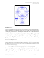
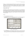
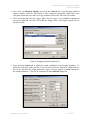
Geosensing Engineering and Mapping (GEM)
Civil and Coastal Engineering Department
University of Florida
ALSM Data Processing
GEM Center Report No. Rep_2004-06-001
M. Sartori, M. Starek, K.C. Slatton
June 3, 2004
© 2004, GEM. All rights reserved
Point of Contact:
Prof. K. C. Slatton
University of Florida; PO Box 116130; Gainesville, FL 32611
Tel: 352.392.0634, Fax: 352.392.0044, E-mail: [email protected]
Geosensing Engineering and Mapping (GEM)
University of Florida
ALSM Data Processing
1.0 Introduction
During a survey the following data sets are collected: multiple base station GPS data, onboard
GPS data, laser and IMU data. After the data sets are retrieved from the GPS units and the laser
system, ALSM data processing is conducted. ALSM processing consists of the following basic
steps:
1. Process the plane navigation data relative to multiple base station references
2. Combine the navigation data with the IMU data and process
3. Combine the navigation-IMU data with the laser data and process to output format
4. Post process to create project deliverables (e.g. DEM)
2.0 Processing of Navigation Data
The initial step in processing ALSM observations is to compute points along the trajectory of the
aircraft using phase-differenced kinematic techniques to determine the aircrafts position during
the survey [2]. First, a reference coordinate is processed for the ground station/s relative to a
control reference. The desired reference control is something local from the region. Published
coordinates are normally not utilized. Rather, the project GPS receivers are generally processed
to the CORS reference stations, often 50-200km distant, utilizing NOAA’s on-line processor,
OPUS.
CORS and OPUS
The National Geodetic Survey (NGS), an office of NOAA, coordinates a network of
Continuously Operating Reference Stations (CORS) that provide GPS carrier phase and code
range measurements in support of three-dimensional positioning activities throughout the US and
its territories. CORS data can be applied to position points where GPS data have been collected
enabling positioning accuracies that approach a few centimeters relative to the National Spatial
Reference System, both horizontally and vertically [5].
The On-line Positioning User Service (OPUS) is an on-line processing system developed by
NGS and NOAA that allows users to upload their GPS data files via the Internet to NGS, where
the data is processed to determine a position using NGS computers and software. Each data file
that is submitted is processed with respect to 3 CORS sites that are selected based upon distance
from the station, number of observations, site stability, and other criteria. OPUS is an automatic
system and requires the following information from the user [6]:
• The email address where you want the results sent
• The data file that you want to process
• The antenna type used to collect this data file (selected from a list of calibrated GPS
antennas)
• The height of the Antenna Reference Point (ARP) above the monument or mark that you
are positioning
GEM_Rep_2004_06_001.doc
p. 2 of 13
Geosensing Engineering and Mapping (GEM)
University of Florida
• As an option, you may also enter the state plane coordinate code if you want SPC
northing and easting.
• As an option, up to 3 base stations may be selected for use in determining your solution.
The data file to be processed is uploaded to OPUS in RINEX format. Multiple files may be
submitted in a zip archive, but your selected options will be applied to all of the files in the
archive. OPUS will only process dual-frequency, carrier-phase data (L1 & L2). Only data from
a dual-frequency receiver may be submitted. Single frequency data (L1 only) will not be
processed. The data must have been collected from a stationary receiver and for a minimum of 2
hours [6].
After the data file is uploaded, OPUS will process it and provide a solution file for the position
of your receiver via email in both ITRF and NAD83 coordinates as well as UTM, USNG and
State Plane Coordinates (SPC) northing and easting [6]. The NAVD88 (GEOID99) datum is
probably utilized most often, and occasionally, the NAD83 datum is utilized where the vertical
datum is ellipsoid height based upon the NAD83 ellipsoid, WGS84 (i.e. GRS80). However, the
datums utilized vary and are dependent on the project.
Aircraft Trajectory
After a reference coordinate has been determined, the precise plane trajectory is computed by
processing the onboard kinematic (moving) GPS data relative to the static base station’s
reference coordinate using the KARS program developed by Dr. Gerry Mader of NOAA [4].
One should try and utilize the precise orbits for the GPS satellites for processing of the trajectory
solution rather than the broadcast orbit, which is a predicted orbit. Agencies that provide precise
orbit values for the GPS satellites include JPL and the Naval Observatory.
For each reference base station, the trajectory of the plane is processed relative to that station to
perform QA/QC analysis of the trajectory. The trajectories relative to each base station are
differenced and compared to determine if essentially the same trajectories were computed. Large
differences between the trajectories indicate a potential problem and/or error in the processing
and corrections must be implemented.
Error targets are in the range of less than 1 to 2 cm horizontally and 2 to 3 cm vertically on a
second by second basis. Generally, one strives for 90% of differenced values to be less than + or
– 5 cm vertically and + or – 2 cm horizontally. If the ranges are within acceptable limits and one
is confident in the quality of the trajectories, a trajectory for the plane can then be selected.
Usually the trajectory relative to the base station with the minimum baseline to the aircraft is
selected; however, the selected trajectory can change dependent upon survey characteristics and
changes in the current region of interest.
Summary
Essentially, the entire processing sequence for determining the plane trajectory is computed
utilizing NOAA software. The CORS network and the OPUS system are used to process
GEM_Rep_2004_06_001.doc
p. 3 of 13
Geosensing Engineering and Mapping (GEM)
University of Florida
reference coordinates for each static base station, and the KARS program is utilized to process the
kinematic GPS solution relative to each static base station’s reference coordinate.
3.0 Processing of IMU Data
After determining a high-confidence trajectory, the next phase in ALSM processing is to
combine the trajectory data with the IMU data utilizing the Applanix POSProc tools.
Description of POSProc
POSProc stands for Position and Orientation System post-PROCessing. It comprises a set of
software tools that interact together to compute an optimally blended navigation solution of the
planes trajectory from inertial data and aiding sensor data [1]. The inertial data comes from the
ALSM onboard IMU system and the onboard firmware designed by Optech. The aiding sensor
data for this discussion refers to the GPS trajectory solution from section 2.0 above.
The POSProc system architecture consists of an integrated inertial navigation module (iin) and a
smoother module (smth) that work symbiotically to produce a Best Estimate of Trajectory. The
most widely used iin configuration is a closed-loop aided inertial navigation architecture that
consists of a feedback error controller, strapdown navigator, and Kalman filter. The Kalman
filter processes measurements that match the strapdown navigation solution with the aiding
sensor data to obtain estimates of the significant errors in the navigation instruments [1].
Typical error characteristics of the inertial navigator are Schuller oscillations and a position error
that grows linearly with time, compared to the GPS receiver with error characteristics indicative
of broadband noise. The low frequency error of the IMU data and the broadband errors of the
aiding sensor GPS data are complementary. The Kalman filter uses the complementary nature of
these error characteristics to calibrate the inertial errors and aiding sensor errors against each
other [1].
iin computes an optimally accurate navigation solution at each time point based on the
information provided for all past and current input data. The closed-loop error control algorithm
utilizes the estimated errors generated by the Kalman filter to control the errors internal to the
strapdown navigator so that the strapdown navigator output is the blended navigation solution.
The inertial navigator is continuously aligned and its position and velocity errors are regulated to
impose consistency with the accuracies of the aiding sensor data [1].
The smoother module (smth) is a recursive modified Bryson-Frazier smoother that operates on
the Kalman filter data generated by iin and calculates smoothed navigation error estimates that
are more accurate than the navigation error estimates computed by iin. The smoother then uses
the smoothed error estimates to correct the strapdown navigation solution from the iin to which
the Kalman filter’s estimated errors apply thereby generating the Best Estimate of Trajectory
(BET) for the given suite of navigation sensors. This is the most accurate navigation solution
obtainable from the processed IMU and aiding GPS trajectory data [1].
GEM_Rep_2004_06_001.doc
p. 4 of 13
Geosensing Engineering and Mapping (GEM)
University of Florida
It is important to note that there are several POSProc processing configurations other than the
closed-loop error control configuration that can be implemented dependent upon processing
requirements including the feedforward error control configuration and the free-inertial INS
configuration. For an in depth review on POSProc architecture and configuration setups refer to
the POSProc User Manual [1].
Processing with POSProc
In order to combine the trajectory data with the IMU data in POSProc, the trajectory data must
be reformatted into an Applanix binary format. Each trajectory record is formatted to an 80byte record based on C-language language data types. Each IMU record can be formatted to
either a 32-byte integer type record or a 56-byte floating-point type record, both of which are
based on C-language data types. Refer to the POSProc User Manual for details on input file
format [1].
After the data is properly formatted, the files are input into POSProc for processing. The
generated output is a 50hz position and orientation “sbet” file containing the blended navigation
solution for the trajectory based on the IMU and aiding sensor data.
Validating the Navigation Solution
POSProc essentially acts as a black box processor where the user provides the IMU and GPS
differential specifications and the software outputs a solution. POSProc provides tools to
analyze errors generated during the Kalman filtering process. These tools allow one to validate
results and compare differences in output dependent upon the Kalman filter mode selected.
When the “sbet” file is validated and determined acceptable, the processing of the aircraft
navigation is completed.
4.0 Processing of Navigation and Laser Data
Processing of the navigation and laser data is performed with the REALM software set of tools.
REALM is the main laser-processing software developed by Optech. The “sbet” file containing
the navigation solution is imported into REALM along with the laser range-file. The laser rangefile contains the scanner mirror angles, laser ranges, and time stamps. The range-file is
downloaded from the onboard removable hard drive and imported directly into the REALM
software.
Description of REALM
REALM (Results of Airborne Laser Mapping) is a modular survey software suite for processing
of the raw laser data derived from the Optech ALTM sensor. REALM was designed to work with
the complete range of ALTM systems, and it enables one to download, convert, and manipulate
airborne laser data. The processed data files can then be brought into an “off-the-shelf”
visualization package for graphic representation and product output [7].
GEM_Rep_2004_06_001.doc
p. 5 of 13
Geosensing Engineering and Mapping (GEM)
University of Florida
REALM produces three-dimensional point data acquired by the ALTM. These are processed
from various inputs including: laser ranges, intensity values, scan angles, differential GPS data,
inertial navigation data, and system calibration data. Classification and output algorithms allow
for the controlled output of the 3D point data into different types including ground or vegetation
only, time sequential, flight line, comprehensive format output, patches (input for DEM
generation), buildings (3D city modeling), and power lines [7].
REALM provides a graphical user interface to interact with different tool components of the
software (e.g. Geodetic tools, GPS tools, INS tools, ALS tools). The modular structure ensures
that the various tools are connected to each other providing controlled process flow. Figure 1
below displays the basic processing steps of REALM. Figure 2 below displays the processing
flow among the various modules in REALM [7].
Figure 1: REALM Basic Processing [7]
GEM_Rep_2004_06_001.doc
p. 6 of 13
Geosensing Engineering and Mapping (GEM)
University of Florida
Figure 2: REALM Processing Flow [7]
REALM Processing
Laser processing in REALM is based upon area-polygons defined by the user. REALM provides a
graphical representation of the flight lines for the survey area thereby allowing the user to select
a given region for processing by highlighting the region with a user-defined polygon. This
functionality allows the user to group areas of close spatial proximity together for processing
rather than having to process the entire survey region as a whole; however, if desired, the entire
survey area can be processed by defining a polygon to encompass all flight lines. Polygons are
selected dependent upon project requirements and characteristics of the survey region such as
spatial proximity of flight lines, size of the survey area, specific regions of interests defined by
the client, etc.
Comprehensive Output Format
After selecting a region for processing by defining an area-polygon, REALM processes the region
and outputs a final output format. In the past, the most used output format provided by REALM
was a 9-column format as follows:
[time stamp, x2, y2, z2, last return intensity, x1, y1, z1, first return intensity]
However, a paradigm shift is occurring. REALM provides a new data format called the
comprehensive format, and the paradigm shift is towards the utilization of this new
comprehensive format. The user can select REALM to have the data processed and output with
the “comprehensive” computing mode. The data will be output to a file with a “.CMP”
GEM_Rep_2004_06_001.doc
p. 7 of 13
Geosensing Engineering and Mapping (GEM)
University of Florida
extension. The file name is automatically assigned by REALM. The comprehensive format
requires an extensive amount of disk space: for example, over 9 mb/sec for a 50khz ALTM
system [7]. The header format is presented in Figure 3 and the record format is presented in
Figure 4.
Figure 3: Comprehensive Header Format [7]
Figure 4: Comprehensive Record Format [7]
GEM_Rep_2004_06_001.doc
p. 8 of 13
Geosensing Engineering and Mapping (GEM)
University of Florida
From the above it is apparent that the comprehensive format provides return intensities for
intermediate values as well as the first and last return; however, the GEM ALTM system only
provides 1st and last return intensities. Intermediate returns are only provided by the latest
Optech systems. Refer to the REALM data processing manual for an in-depth discussion on the
comprehensive format and software utilization [7].
5.0 Post Processing
Once the navigation and laser data have been processed with REALM, the data is in a usable,
“final” format, which then can be directly utilized or further processed. Depending on the
application and project requirements, the data can be post processed for creation of specific
project deliverables. In most instances, the required project deliverable for the client is a bare
earth digital elevation model (DEM).
Gridding with Surfer
The generation of DEMs is accomplished with Surfer. Surfer is a contouring and 3D surface
visualization and mapping program that can convert XYZ data files into contour, surface,
wireframe, vector, image, shaded relief, and post maps. The most common application of Surfer
and the importance of Surfer for this example is its ability to create a grid-based data file from an
irregular spaced XYZ data file [3].
Gridding methods produce a regularly spaced, rectangular array of Z-values (heights) from
irregularly spaced XYZ data. The term "irregularly spaced" means that the points follow no
particular pattern over the extent of the region, resulting in many "holes" where data are missing.
Gridding fills in these holes by interpolating Z-values at those locations where no data exist. The
grid that is formed is a rectangular region comprised of evenly spaced rows and columns. The
intersection of a row and column is called a grid node, and gridding generates a Z-value at each
grid node by interpolation [3].
Surfer provides many different gridding methods for interpolation of the data. Different gridding
methods provide different interpretations of the data because each method calculates grid node
values using a different algorithm. Some methods are better than others in preserving the data,
and sometimes some experimentation is necessary before one can determine the optimal method
for the data. Gridding methods provided by Surfer include Inverse Distance to a Power, Kriging,
Minimum Curvature, Modified Shepard's Method, Natural Neighbor, Nearest Neighbor,
Polynomial Regression, Radial Basis Function, Triangulation with Linear Interpolation, Moving
Average, Data Metrics, and Local Polynomial [3].
Kriging
The method utilized for gridding of the processed ALTM laser data is Kriging. Kriging is a
geostatistical gridding method that can produce accurate, optimally gridded data points from
irregularly spaced data. The statistical properties of Kriging attempt to model trends suggested in
the data, so that, for example, high points might be connected along a ridge rather than isolated
by bull's-eye type contours [3].
GEM_Rep_2004_06_001.doc
p. 9 of 13
Geosensing Engineering and Mapping (GEM)
University of Florida
Kriging is a very flexible interpolation method that can be custom-fit to a data set by specifying
an appropriate variogram model within Surfer. Kriging incorporates anisotropy and underlying
trends, and the user can adjust the anisotropy parameters to better suit the data. In addition,
Kriging can operate as either an exact or a smoothing interpolator depending on the parameters
selected by the user in Surfer [3].
Creating a DEM in Surfer
The following is an example workflow of the steps taken within Surfer to create a DEM utilizing
the Kriging interpolation method. It is important to note that this example assumes that the data
has been completely processed and filtered before importing into Surfer. Therefore, any filtering
such as vegetation and structure removal for generation of bare-earth DEMs must be completed
prior to conducting the gridding process in Surfer outlined below. Refer to the GEM report on
“filtering” for details.
In Surfer:
1. Click on Grid | Data from the file menu.
2. In the Open dialog, select the data file containing the XYZ values of the processed laser data
and then click the Open button. A Grid Data dialog display will open similar to below.
Figure 5: Grid Data Dialog [3]
3. In the Grid Data dialog, select the appropriate columns for the X, Y, and Z-values from the
data file. Select Kriging in the Gridding Method group, select the desired spacing, range, and
size of the grid in Grid Line Geometry fields, and select a location for the Output Grid File.
GEM_Rep_2004_06_001.doc
p. 10 of 13
Geosensing Engineering and Mapping (GEM)
University of Florida
4. Next, click on Advanced Options and select the General tab on the Kriging advanced
options window. Click the Add button to add variogram components. Select the Linear
variogram, adjust the slope and anisotropy parameters if need be, and click OK to add it.
5. Click Add again and select the Nugget Effect. Set the variance to 0 (standard configuration
but can be adjusted) and click OK to add the Nugget Effect. The display should now be
similar to below.
Figure 6: Krigging Advanced Options [3]
6. Next, select the Search tab to adjust the search capabilities of the Kriging algorithm. To
utilize all of the data, make sure the No Search box is checked. Otherwise, uncheck the No
Search box and enter the search parameters. Figure 7 below displays a standard format for
the search parameters. Click OK to return back to the Grid Data dialog box.
GEM_Rep_2004_06_001.doc
p. 11 of 13
Geosensing Engineering and Mapping (GEM)
University of Florida
Figure 7: Standard Values for Search Parameter [3]
7. After the advanced options and parameters have been set, click OK on the Grid Data dialog
box and the DEM will be generated utilizing the defined Kriging parameters.
The above is only a general outline of the steps in Surfer to generate a DEM and may vary
dependent upon the data being processed and the parameters utilized. There are numerous
Kriging parameters that can be adjusted or refined and it may be necessary to experiment with
different settings until a desired result is found. Most gridding is automated within Surfer
performed by scripts. Refer to the Surfer User Manual for further detail [3].
Appendix A
Table of Software:
Software
Online Positioning
User System (OPUS)
POSPac version 4.02
REALM version 3.2
Surfer version 8.03
Maker
NOAA – NGS - 2004
Application
Processing of GPS base stations with CORS
Applanix – 2002
Processing of IMU and trajectory with
POSProc module contained in POSPac 4.02
Optech – 2003
Processing of navigation and ALTM laser
data
Golden Software, Inc. – Generation of DEMs
2003
References
[1] Applanix, POSProc User Manual Version 2.1, Applanix Corporation, Revision: 2, March
1997.
[2] Carter, W.R.; R. Shrestha; G. Tuell; D. Bloomquist; and M. Sartori, “Airborne Laser Swath
Mapping Shines New Light on Earth’s Topography,” Eos, Transactions, American Geophysical
Union, Vol. 82, No. 46, Nov. 2001, Pages: 549-555, 2001.
[3] Golden Software, Surfer Version 8.03 – User Guide, Golden Software, Inc., May 2003.
[4] Mader, G.L., "Rapid Static and Kinematic Global Positioning System Solutions Using the
Ambiguity Function Technique," Journal of Geophysical Research, 97, 3271-3283, 1992.
[5] NOAA, “National Geodetic Survey – What is CORS?” http://www.ngs.noaa.gov/CORS/corsdata.html, accessed June 2004.
[6] NOAA, “OPUS – What is OPUS?” http://www.ngs.noaa.gov/OPUS/What_is_OPUS.html,
accessed June 2004.
GEM_Rep_2004_06_001.doc
p. 12 of 13
Geosensing Engineering and Mapping (GEM)
University of Florida
[7] Optech, REALM Survey Suite Data Processing Manual - ALTM, Optech Inc., Document No.:
195-090-06, Release: 3.1, Oct. 2002.
GEM_Rep_2004_06_001.doc
p. 13 of 13