1
Aalborg Universitet
Elektronik og Elektroteknik
Fredrik Bajers Vej 7
DK-9200 Aalborg
Tlf. (+45) 9940 8600
http://www.es.aau.dk
Title:
Low Complexity Pruning FFT
Algorithms
Theme:
DSP Algorithms and Architectures
Project period:
E8, Spring term 2008
Project group:
840
Participants:
Mads Lauridsen
Matthieu Noko
Niels Lovmand Pedersen
Supervisor:
Anders B. Olsen
Jesper M. Kristensen
Copies: 6
Number of pages: 141
Attachment: CD
Finished: June 2nd 2008
The content of this report is freely
accessible, though publication
(with reference) may only occur
after permission from the authors.
Abstract:
The objective of this project is to analyse low
complexity Fast Fourier Transform (FFT) algorithms. The target is the pruning FFTs that only
operate on the utilized frequency spectrum. The
pruning FFTs are analysed and compared with
the conventional FFTs with regards to execution
time and resource usage.
The analysis has been performed in Matlab and
on the Altera DE2 board. Based on a review of
articles a split-radix algorithm was selected for
further analysis. The split-radix FFT was pruned
and a computation count, based on a Matlab implementation, shows that up to 55 % multiplications are saved when 50 % of the outputs are
pruned as compared to the conventional splitradix FFT.
Three different implementations were made on
the Altera DE2 board and analysed using the
Quartus II Software Suite. A SW and a HW/SW
implementation were created using a Nios II softcore processor system and the algorithms were
coded in C using the IDE Nios II and accelerated with the C-to-HW compiler. A HW implementation was developed using the Altera DSP
Builder, which is a plugin to Matlab’s system
builder Simulink.
The SW and HW/SW implementations were
implemented successfully, but reliable execution
time measurements were not obtained. In the
HW solution the pruning control structures were
implemented in parallel with the arithmetic operations of the split-radix FFT, which entails
that performing the control structures are costless with regards to the overall execution time.
The resource usage was only increased with 8 %
point extra memory. The time savings reflected
the computation count in Matlab.
The pruning split-radix FFT has shown to be
computationally and time efficient. A further
implementation could analyse the pruning splitradix FFT over several time slots, since this
project focused on a single time slot.
Mads Lauridsen
ii
Matthieu Noko
Niels Lovmand Pedersen
Preface
This report is written during the 8th semester specialisation in Applied Signal Processing and
Implementation at the department of Electronic Systems. According to the study guidelines
the the student should be able to demonstrate [2, p. 29]:
• That she can apply methods for specification, representation, analysis, and transformation/modification of digital signal processing algorithms for either signal modification,
-analysis, or -transmission.
• That she can apply methods for optimizing the interaction between DSP algorithms and
appropriate real-time architectures - either software-programmable processors or application specific HW-architectures. The student should be able to evaluate and improve
the interaction primarily in terms of execution time and/or memory usage.
This report will cover analysis, implementation and test of FFTs and pruning FFTs in Matlab
and on the Altera DE2 board. The objective of this report is to compare pruning FFTs and
standard FFTs with regards to execution time and resource usage. Based on the tested pruning
FFTs the report suggests methods for optimizing the pruning with regards to the number of
used computations and execution time.
References are represented with numbers, e.g. [number], and the full list of references is
found in the Bibliography section. In the chapter ”Hardware Solution”, modules representing
different system blocks are represented with the notation system block. The same notation
is used for the signal names. Arguments are represented with italic, e.g. i.
The enclosed CD contains the following:
• The report in PDF format P8.pdf.
• The source code for the algorithms in Matlab.
• The source code for the algorithms in C.
• The Nios II softcore processor system.
• The Simulink models containing the implementation.
• Literature containing articles from Altera.
The group would like to thank Assistant Professor Yannick Le Moullec for his help with the
implementations on the Altera DE2 board.
iii
iv
Contents
I
Introduction
1 Introduction
II
1
3
1.1
Initiating Problem Statement . . . . . . . . . . . . . . . . . . . . . . . . . . . .
5
1.2
Performance and Complexity . . . . . . . . . . . . . . . . . . . . . . . . . . . .
6
Analysis
9
2 DFT and FFT
11
2.1
Radix-2 FFT . . . . . . . . . . . . . . . . . . . . . . . . . . . . . . . . . . . . .
11
2.2
Radix-4 FFT . . . . . . . . . . . . . . . . . . . . . . . . . . . . . . . . . . . . .
15
2.3
Split-Radix FFT . . . . . . . . . . . . . . . . . . . . . . . . . . . . . . . . . . .
17
2.4
The Implemented Split-Radix FFT . . . . . . . . . . . . . . . . . . . . . . . . .
19
3 Pruning FFT
23
3.1
General Pruning FFT . . . . . . . . . . . . . . . . . . . . . . . . . . . . . . . .
24
3.2
Computation Count . . . . . . . . . . . . . . . . . . . . . . . . . . . . . . . . .
28
4 Available HW/SW
37
4.1
Available Hardware . . . . . . . . . . . . . . . . . . . . . . . . . . . . . . . . . .
37
4.2
Available Software . . . . . . . . . . . . . . . . . . . . . . . . . . . . . . . . . .
40
5 Problem Statement
43
v
CONTENTS
III
Design, Implementation and Test
6 SW and HW/SW Solution
47
6.1
Design . . . . . . . . . . . . . . . . . . . . . . . . . . . . . . . . . . . . . . . . .
47
6.2
Implementation . . . . . . . . . . . . . . . . . . . . . . . . . . . . . . . . . . . .
54
6.3
Test . . . . . . . . . . . . . . . . . . . . . . . . . . . . . . . . . . . . . . . . . .
56
6.4
Discussion and Further Development . . . . . . . . . . . . . . . . . . . . . . . .
61
7 Hardware Solution
IV
45
63
7.1
Design . . . . . . . . . . . . . . . . . . . . . . . . . . . . . . . . . . . . . . . . .
63
7.2
Implementation . . . . . . . . . . . . . . . . . . . . . . . . . . . . . . . . . . . .
68
7.3
Test . . . . . . . . . . . . . . . . . . . . . . . . . . . . . . . . . . . . . . . . . .
89
7.4
Discussion and Further Development . . . . . . . . . . . . . . . . . . . . . . . .
92
Conclusion and Future Development
95
8 Conclusion
97
9 Future Development
99
Bibliography
101
V
103
Appendix
A Orthogonal Frequency Division Multiple Access
105
B The Split-Radix Algorithm
107
C Algorithms for the Pruned FFTs
111
D Split-Radix Example
115
E Implemented Simulink Models
125
F Tests of Implementations
127
vi
F.1 Test of SW Solution . . . . . . . . . . . . . . . . . . . . . . . . . . . . . . . . . 127
F.2 Test of HW/SW Solution . . . . . . . . . . . . . . . . . . . . . . . . . . . . . . 129
F.3 Test of HW Solution . . . . . . . . . . . . . . . . . . . . . . . . . . . . . . . . . 130
Part I
Introduction
1
1
Introduction
In this project the focus is on analysis, design and implementation of various forms of the
Fast Fourier Transform (FFT). One of many applications for the FFT is in communication
systems. Mobile phones, laptops, ADSL, radios and even TVs apply different communication
technologies. To fulfill the requirements to quality of information, new modulation schemes are
utilized. One of them is the Orthogonal Frequency Division Multiplexing (OFDM) modulation
scheme which divides the available frequency band into subchannels by the use of orthogonal
subcarriers. Because of the orthogonality the carriers can be placed very close to each other
without corrupting the information, thus improving spectral efficiency. The OFDM scheme
applies an Inverse Fast Fourier Transform (IFFT) algorithm to generate the orthogonal signals
in the transmitter and an FFT algorithm in the receiver.
An interesting application based on OFDM is when multiple users can access the subchannels of the channel. This scheme is called Orthogonal Frequency Division Multiple Access
(OFDMA). It allows users with different bandwidth and modulation requirements to use one
or more subcarriers while users with other requirements use other parts of the channel. This
is illustrated in figure 1.1 which also shows that the multiple user signals can be separated in
time and/or frequency. In appendix A the theory of OFDMA is elaborated.
3
Introduction
Figure 1.1: An OFDMA signal in the time and frequency domains. [24, Figure 3].
The advantage of OFDMA is that the users can choose subcarriers on basis of the channel’s
frequency spectrum. If for example the channel attenuates low frequencies at time t1 then
the transmitter will choose subcarriers at higher frequencies. Later at time t2 the situation
might change, e.g. if the user is moving, so that low and high frequencies have higher gain
than those in between. Then the transmitter will utilize separated subcarriers with low and
high frequencies. When the transmitter changes the subcarrier(s) for the user, it is said to
perform subcarrier allocation. The aim with the allocation is to make sure that the users get
a channel with a flat frequency response and low attenuation.
In the case of multiple users, subcarrier allocation is useful when a given subcarrier is unfit for one user (because of high attenuation) and applicable for another user, because the
channel conditions are better from the second users location. This is called multiuser diversity. Allowing multiple access will entail that not all subchannels always are used. This means
that the FFT in the receiver will operate on subcarriers that do not contain information targeted for the user. To avoid this the transmitter, which performs subcarrier allocation, will
notify the receiver about the utilization of the channel i.e. which channels are used in the
current time slot. When the receiver learns that some subchannels are unused, pruning FFT
algorithms can be applied. The idea with these algorithms is that they only operate on subchannels containing useful information aimed at the user.
In this project it is investigated whether pruning FFT algorithms yield performance improvements compared to conventional FFT algorithms or not. A performance improvement can be
equated with lower complexity which again is assumed to lead to e.g. lower power consumption, which is desirable. The pruning algorithms may however not reduce the complexity if
they require too many control structures that determine the subcarriers the algorithm should
operate on.
An obvious application for pruning FFTs is the OFDMA system. The project however will
not contain further analysis of OFDMA, but it is a suggested application for the developed
pruning FFTs.
4
1.1 Initiating Problem Statement
1.1
Initiating Problem Statement
A fundamental part of the OFDMA receiver is the FFT. Another aspect is that a subchannel,
of the OFDMA system, may not be utilized. This introduces the pruning FFT that only
operates on the utilized part of the spectrum. In this project the FFT will be analysed under
different scenarios to investigate when the pruning FFT may perform better and is less complex than the traditional FFT. The analysis of the FFT and the pruning FFT will therefore
be the scope of the project.
The pruning FFT needs control structures to adapt to the corresponding subcarriers not
being used. For measuring the complexity of pruning FFTs it must therefore be analysed how
control structures affect the complexity.
Power
It can be suggested that due to the complexity of an adaptive pruning FFT, a normal FFT
would perform better if there is only a few holes (unused subcarriers) in the frequency spectrum. Various cases for the FFT are therefore needed when the performance of the FFT and
pruning FFT algorithms are analysed. These cases are:
• Fixed holes in the spectrum that do not change over time. The pruning FFT
operates
Subchannel
1
Subchannel
2
on the same subcarriers and does not adapt to new scenarios with changing
subcarriers
Subchannel 3
for different time slots.
No subchannel
• Non-fixed holes in the spectrum that do change over time. The pruning FFT must be
able to adapt to the different subcarrier allocation for different time slots.
Frequency
Subchannel 1
Subchannel 2
Power
Power
Both cases should be investigated with adjacent subcarrier method (ASM) and diversity subcarrier method (DSM) subcarrier allocation. These methods are illustrated in figure 1.2
Subchannel 1
Subchannel 2
Subchannel 3
Subchannel 3
No subchannel
No subchannel
Frequency
Frequency
(a) Adjacent subcarrier method (ASM)
(b) Diversity subcarrier method (DSM)
Power
Figure 1.2: The ASM and DSM subcarrier allocation techniques
Subchannel 1
The ASM method is in this report defined
Subchannelas
2 subcarrier allocation, where used subcarriers are
Subchannel
3
allocated adjacent. The same applies
for subcarriers
that are not used (hence also referred to
No subchannel
as holes in the frequency spectrum). DSM allocation is defined as used subcarriers that are
not necessarily located in continuation of each other and furthermore unused subcarriers may
be in between the used ones.
Frequency
Limitations
The scenarios will not have any focus on channel conditions. It is assumed that subcarrier
allocation, modulation and bit loading for each of the subcarriers are in place. Furthermore
due to the time constraints of one academic semester the analysis will be restricted to one time
5
Introduction
slot meaning that the analysis will only concern fixed holes in the spectrum that do not change
over time. This case will be analysed with respect to ASM and DSM subcarrier allocation.
The next analysis made in another project should analyse the complexity and performance of
the FFT and pruning FFT when they need to adapt to a system where subcarrier allocation
changes over time.
Before the analysis of normal and pruning FFTs a definition of the performance metric is
needed. Furthermore the term complexity, which influence the performance needs to be defined.
1.2
Performance and Complexity
The main performance factor that the project group wants to analyse the FFTs with respect
to is execution time measured in either seconds or clock cycles. The other factor is the resource
requirements the pruning algorithms introduce. Resources are referred to as: logic elements,
registers, arithmetic operators (multipliers, adders etc.), and memory. These are all components that will increase the area of the system.
Another interesting performance factor is energy usage. The question is whether or not the
pruning algorithms will increase the power usage of the system if the resource usage is increased. The power usage is however not a factor, which the group can elaborate on because
of the time limitations of a single semester. The performance metrics for the pruning FFTs
are therefore time and area.
The assumption is that lowering the amount of computations used by a FFT by pruning it,
will lower the execution time. Pruning will introduce control structures for deciding whether
pruning must be performed or not. These control structures are not costless with regards
to time or resources used. It is therefore interesting to analyse what the relationship between lowering the amount of computations and the introduction of extra control structures
is. Therefore complexity is defined as computations and control because these are the factors
that influence the defined performance metric. Complexity is a big research area and other
standards could have been examined and used. The objective is to compare the algorithms
and for that counting the computations and measuring the resource usage is sufficient.
In the analysis it shall be investigated if pruning could increase the complexity and thereby
the execution time, even though computations are saved, due to the extra control structures
introduced in the pruning algorithms. The opposite situation where pruning is implemented
in such a way that even though no computations are saved, then the added control structures
will not increase the execution time compared with an normal FFT, must also be examined.
In other words this means control structures are costless with respect to execution time and
only introduce use of extra resources.
The complexity of the pruning FFT algorithms influence on performance is analysed in two
parts of the report:
• The amount of saved computations when using pruning FFTs will be analysed for different algorithms in Matlab.
• Execution time and required resources for pruning FFTs will be analysed on a HW and
6
1.2 Performance and Complexity
SW platform.
After the analysis in Matlab one pruning FFT algorithm will be chosen for further implementation and analysis on a HW and SW platform. The analysis in Matlab will lead to a
problem statement which first will summarize the results obtained in Matlab, and then give
the problem statement for the analysis of the implementation in HW and SW.
7
Introduction
8
Part II
Analysis
9
2
DFT and FFT
In the OFDMA system the Discrete Fourier Transform (DFT) is needed to ensure orthogonality between subcarriers. The DFT, as shown in this chapter, is computational heavy and
for optimizing the OFDMA system it is necessary to make the DFT faster - hence the number
of computations should be lowered. In this chapter the methods Decimation-In-Time (DIT)
and Decimation-In-Frequency (DIF) will be introduced for obtaining the Fast Fourier Transform (FFT). This will lead to two types of the so called butterflies - DIT and DIF butterflies,
which forms the structure of the DIT and DIF FFT flow graphs respectively. For FFTs with
the length of a radix-2 number, it will be shown that these two butterflies share duality corresponding to that they are a mirrored version of each other, which makes the structure of
radix-2 FFT flow graphs very flexible. The flow graphs of radix-4 and split-radix FFTs will
also be given showing that the split-radix FFT is superior to the radix-2 and radix-4 FFT but
has a more complex flow graph. Lastly an implemented split-radix FFT will be presented.
2.1
Radix-2 FFT
The Discrete Fourier Transform (DFT) is a Fourier Transform which is discrete in time and
frequency. The DFT of the sequence x[n] of N points is defined by, [19]
PN −1
kn
0≤k ≤N −1
n=0 x[n]WN
X[k] =
(2.1)
0
otherwise
where:
X[k] is the (complex) sequence in discrete frequency
x[n] is the (complex)
sequence in discrete time
2π
WN = exp −j N is the primitive root of unity (also called the twiddle factor)
k is the frequency index, k = 0, 1, ..., N − 1
n is the time index, n = 0, 1, ..., N − 1
From (2.1) it can be seen that N complex multiplications and N − 1 complex additions is performed for each k corresponding to approximately N 2 complex multiplications and additions
11
[-]
[-]
[-]
[-]
[-]
DFT and FFT
for computing the DFT. The approach for reducing the number of computations and deriving
the FFT can be divided into two methods: Decimation-In-Time and Decimation-In-Frequency.
The two methods are both based on the same approach shown in figure 2.1. First this general
approach is described then an example is given for deriving the DIT DFT. Then the DIF FFT
is presented followed by a comparison of the two methods.
As illustrated in figure 2.1 the N-point DFT is first divided into two parts.
Stage number
N-point DFT
1
N/2-point DFT
(even index)
2
N/4-point DFT
3
N/4-point DFT
N/4-point DFT
2-point DFT
.....
2-point DFT
N/4-point DFT
.....
.....
.....
m = log2(N)
N/2-point DFT
(odd index)
2-point DFT
2-point DFT
Figure 2.1: Decomposition approach for the radix-2 DFT.
If the DIT method is used the time sequence x[n] is divided into even and odd components.
For DIF it is the frequency sequence X[k] that is divided into even and odd components. These
two N2 -point DFTs are then divided into four N4 -point DFTs. This decomposition is performed
until only 2-point DFTs occur, hence the decomposition must be performed m = log2 N times.
The number of computations are lowered if the mapping from the N -point DFT down to 2point DFTs and the computations required in the 2-point DFT are less than performing the
N -point DFT directly. This can also be described as [15, p. 265]
X
2.1.1
cost(subproblems) + cost(mapping) < cost(original
problem)
(2.2)
Decimation-In-Time
For the N = 8 point DFT the time sequence is first divided into even and odd indexes, [19].
X[k] =
=
7
X
n=0
3
X
x[n]WNnk
x[2p]WN2pk +
p=0
=
3
X
3
X
(2p+1)k
x[2p + 1]WN
p=0
pk
x[2p]WN/2
+ WNk
p=0
= G[k] +
12
,0 ≤ k ≤ 7
3
X
pk
x[2p + 1]WN/2
p=0
WNk H[k]
(2.3)
2.1 Radix-2 FFT
Using the fact that
−j2π 2
−j2π
= e N/2 = WN/2
WN2 = e N
(2.4)
For X[k] k = {0, ..., 7} but G[k] and H[k] are FFTs of length N/2 = 4 and therefore periodic
in k = 4 and for these k = {0, 1, 2, 3}.
Decomposing G[k] further gives
G[k] =
3
X
pk
x[2p]WN/2
p=0
=
1
X
x[4r]W2rk
+
W4k
r=0
1
X
x[4r + 1]W2rk
r=0
= T [k] +
W4k M [k]
(2.5)
Now T [k] and M [k] are periodic in N/4 = 2 with k = {0, 1}. T [k] is given as (hence X[k] has
been decomposed from stage 1 to log2 (8) = 3)
T [k] =
1
X
x[4r]W2rk
r=0
= x[0] + x[4]W2k
(2.6)
So for k = {0, 1} T [0] and T [1] can be expressed as
T [0] = x[0] + x[4]W20
T [1] = x[0] + x[4]W21 = x[0] − x[4]W20
(2.7)
Using that
W21
2π
= exp −j
2
= −1
It is seen that the two nodes x[0] and x[4] have an index distance of
form the DIT butterfly structure of the 2-point FFT in figure 2.2.
N
2
= 4. The two equations
T [0]
X [0]
X [4]
(2.8)
W20
−1
T [1]
Figure 2.2: DIT butterfly of the 2-point FFT.
The general equations for the 2-point FFT are given below, [19]
Xm [p] = Xm−1 [p] + WNp Xm−1 [p + N/2]
Xm [p + N/2] = Xm−1 [p] +
= Xm−1 [p] −
(2.9)
p+N/2
WN
Xm−1 [p + N/2]
p
WN Xm−1 [p + N/2]
The general butterfly structure is shown in figure 2.3 where q = p +
(2.10)
N
2.
13
DFT and FFT
X m −1[ p ]
X m −1[q ]
X m [ p]
X m [q ]
−1
WNr
Figure 2.3: DIT butterfly of a radix-2 FFT, [19, Figure 9.11].
2.1.2
Decimation-In-Frequency
The Decimation-In-Frequency method follows the same approach as DIT, but now the N -point
DFT is decomposed into N/2 2-point DFTs in frequency. The equations are given followed
by the DIF butterfly structure.
Equation (2.1) can be written as
X[2r] =
X[2r + 1] =
N
−1
X
n=0
N
−1
X
x[n]WNn2r
(2.11)
n(2r+1)
x[n]WN
(2.12)
n=0
The development of the sum of (2.11), makes it possible to use the property of periodicity of
WN
(N/2)−1
X
X[2r] =
x[n]WNn2r +
n=0
X
x[n]WNn2r
n=N/2
(N/2)−1
=
N
−1
X
(N/2)−1
x[n]WNn2r +
n=0
X
2r(n+N/2)
x[n + N/2]WN
n=0
(N/2)−1
X
=
(x[n] + x[n + N/2]) WNn2r
(2.13)
n=0
Since
2r(n+N/2)
WN
= WNn2r WNrN = WNn2r · 1 = WNn2r
(2.14)
Applying the same properties on (2.12), makes it possible to write
N/2−1
X[2r] =
X
nr
(x[n] + x[n + N/2]) WN/2
(2.15)
nr
(x[n] − x[n + N/2]) WN/2
WNn
(2.16)
n=0
N/2−1
X[2r + 1] =
X
n=0
The butterfly structure of the DIF approach is illustrated in figure 2.4.
14
2.2 Radix-4 FFT
X m −1[ p ]
X m [ p]
X m −1[q ]
−1
WNr
X m [q ]
Figure 2.4: DIF butterfly of a radix-2 FFT, [19, 9.21].
2.1.3
Comparison of the DIT and DIF Methods
From figure 2.3 and 2.4 it can be seen that the butterfly structure for DIF is a mirrored
version of the butterfly for DIT and vice versa as stated in the beginning. From figure 2.5,
which shows the flow graph of a 16-point DIF radix-2 FFT, the flexibility of the radix-2 FFT
can be seen. Because of the duality between the DIF and DIT butterflies the DIT FFT could
be obtained by flipping the arrows and performing the bitreverse at the input instead of at the
output. For each stage in the flow graph the butterflies are build with the nodes with index
p and q = p + N/2.
x[0]
x[0]
x[1]
x[2]
W40
-1
W41
x[4]
-1
x[5]
W80
-1
x[6]
W81
-1
-1
x[7]
x[9]
x[10]
x[11]
x[12]
x[13]
x[14]
x[15]
-1
x[12]
-1
x[10]
-1
x[14]
-1
x[9]
-1
x[13]
-1
x[3]
x[8]
-1
x[8]
W82
-1
W40
W83
-1
W41
-1
W160
-1
1
W16
-1
W162
-1
W163
-1
W164
-1
W165
-1
W166
-1
W167
-1
W40
-1
W41
-1
W80
-1
W81
-1
W82
-1
W40
-1
W83
-1
W41
-1
x[4]
x[2]
x[6]
x[1]
x[5]
x[3]
x[11]
x[7]
-1
x[15]
Figure 2.5: Flow graph of the 16-point DIF radix-2 FFT [26, fig. 1(a)].
From figure 2.5 the total computation count can be derived. Each stage has N/2 Butterflies
each requiring 1 complex multiplication and two complex additions. So for an N -point FFT
N
2 log2 (N ) butterflies are computed. One complex multiplication corresponds to 4 real multiplications and 2 real additions, and 1 complex additions corresponds to 2 real additions. For
simplicity, when counting complex multiplications, it will not be distinguished between when
the twiddle factors equals unity or not.
2.2
Radix-4 FFT
This section will introduce the radix-4 FFT, which will be shown for computational comparison. The radix-4 algorithm divides the DFT into twice as many components as the radix-2
15
DFT and FFT
FFT, so any radix-4 FFT can be converted to a radix-2 FFT. The decomposition is now made
for the DIF radix-4 FFT followed by the flow graph.
X[k] =
N
X
x[n]WNnk
n=0
(2.17)
Dividing X[k] into even and odd k indexes gives
X[4r] =
X[4r + 1] =
X[4r + 2] =
X[4r + 3] =
N
−1
X
n=0
N
−1
X
n=0
N
−1
X
n=0
N
−1
X
x[n]WN4rn
=
N
X
rn
x[n]WN/4
(2.18)
n=0
(4r+1)n
x[n]WN
=
(4r+2)n
x[n]WN
=
(4r+3)n
x[n]WN
=
n=0
N
X
n=0
N
X
n=0
N
X
rn
x[n]WNn WN/4
(2.19)
rn
x[n]WN2n WN/4
(2.20)
rn
x[n]WN3n WN/4
(2.21)
n=0
X[4r] is now decomposed into FFTs of length N/4.
X[4r] =
N
X
rn
x[n]WN/4
n=0
N/4−1
=
X
N/2−1
rn
x[n]WN/4
+
n=0
3N/4−1
rn
x[n]WN/4
X
rn
x[n]WN/4
+
N
−1
X
rn
x[n]WN/4
n=3N/4
N/4−1
rn
x[n]WN/4
+
n=0
X
n=N/2
X
r(n+N/4)
x[n + N/4]WN/4
n=0
N/4−1
+
+
n=N/4
N/4−1
=
X
N/4−1
r(n+N/2)
X
x[n + N/2]WN/4
n=0
+
X
r(n+3N/4)
x[n + 3N/4]WN/4
n=0
N/4−1
=
X
rn
(x[n] + x[n + N/4] + x[n + N/2] + x[n + 3N/4])WN/4
(2.22)
n=0
In the last step the properties of the twiddle factor have been used. For example: WNrN = 1
4rN/2
and WN
= 1. For N = 16 X[4r] can be expressed as (hence r = {0, 1, 2, 3})
X[4r] = (x[0] + x[4] + x[8] + x[12])W40
+ (x[1] + x[5] + x[9] + x[13])W4r
+ (x[2] + x[6] + x[10] + x[14])W42r
+ (x[3] + x[7] + x[11] + x[15])W43r
(2.23)
This decomposition must be done for X[4r + 1], X[4r + 2] and X[4r + 3] as well. For N = 16
these four equations form the final flow graph because the equations have then been decomposed into four DFTs with the length of 4. This only required one decomposition where it for
radix-2 required three for N = 8.
In figure 2.6 the flow graph of a 16-point DIF radix-4 FFT is shown.
16
2.3 Split-Radix FFT
x[0]
x[0]
x[1]
x[2]
-1
x[3]
-1
x[4]
-1
x[5]
-1
x[6]
-1
W164
-1
-1
W166
-1
x[7]
x[8]
x[9]
x[10]
x[11]
x[12]
x[13]
x[14]
x[15]
-1
-1
-1
-1
x[12]
-1
x[10]
-1
x[14]
-1
x[9]
-1
x[13]
W160
W162
W160
1
W16
W162
-1
−j
-1
x[8]
W163
−j
-1
-1
-1
−j
-1
−j
W160
-1
-1
-1
−j
W163
-1
-1
-1
−j
W166
-1
W169
-1
−j
-1
x[4]
x[2]
x[6]
x[1]
x[5]
x[3]
x[11]
x[7]
−j
-1
x[15]
Figure 2.6: Flow graph of the 16-point DIF radix-4 FFT [26, fig. 1(b)].
It can be seen when compared to figure 2.5 that it requires less twiddle factors than the radix-2
FFT.
2.3
Split-Radix FFT
Introduced by P. Duhamel and H. Hollmann in 1984 [14], the split-radix FFT mix both radix-2
and radix-4 FFTs to reduce the number of computations. The radix-2 FFT is more efficient
for the even coefficients of the DFT, whereas the radix-4 FFT is used for the odd coefficients
[14]. From the equations for the radix-4 FFT it was seen that the radix-4 FFT needed less
decompositions than the radix-2 FFT. And the radix-4 FFT required less multiplications than
the radix-2 FFT. However from equation (2.15) and (2.16), the radix-2 is divided in two
FFTs of length N/2. The DFT composed by the odd numbers (equation (2.16)), is multiplied
by an additional twiddle factor and it therefore requires more multiplications than the even
term. Therefore the radix-2 FFT is more efficient for the even numbers than the radix-4 FFT,
because it is only equation (2.18), which is not multiplied by any additional twiddle factor.
The equations for the split-radix FFT is given below. Here equation (2.19) and (2.21) are
presented differently by using the properties of the twiddle factors.
N/2−1
X[2r] =
X
nk
WN/2
(x[n] + x[N/2 + n])
(2.24)
nk
WN/4
WNn (x[n] − jx[n + N/4]) − x[n + N/2] + jx[n + 3N/4])
(2.25)
nk
WN/4
WNn (x[n] + jx[n + N/4]) − x[n + N/2] − jx[n + 3N/4])
(2.26)
n=0
N/4−1
X[4r + 1] =
X
n=0
N/4−1
X[4r + 3] =
X
n=0
The even k’s in X[k], equation 2.1, are decomposed into equation (2.24) and odd k’s into
equation (2.25) and (2.26). The choice of (2.25) or (2.26) depends on whether or not k mod
17
DFT and FFT
4 gives 1 or 3. For further decomposition the N/2-point DFT (equation (2.24)) is composed
into one N/4-point DFT and two N/8-point DFTs. The same split-radix approach is made for
the two N/4-point DFTs (equation (2.25) and (2.26)). This decomposition is done until only
2-point DFTs exist in the last stage of the flow graph. The split-radix approach is illustrated
in figure 2.7.
N-point DFT
N/2-point
radix-2 DFT
(even index)
2-point DFT
2-point DFT
N/16-point
radix-4 DFT
(odd index)
N/16-point
radix-4 DFT
(odd index)
.....
.....
2-point DFT
N/8-point
radix-2 DFT
(even index)
.....
.....
2-point DFT
N/16-point
radix-4 DFT
(odd index)
.....
.....
N/16-point
radix-4 DFT
(odd index)
N/8-point
radix-2 DFT
(even index)
.....
N/8-point
radix-4 DFT
(odd index)
.....
N/8-point
radix-4 DFT
(odd index)
.....
N/4-point
radix-2 DFT
(even index)
2-point DFT
N/4-point
radix-4 DFT
(odd index)
N/4-point
radix-4 DFT
(odd index)
2-point DFT
Figure 2.7: The split-radix decomposition approach.
The butterfly of the split-radix FFT, called an L-butterfly, is illustrated in figure 2.8. It can
be seen that the split-radix FFT has a more complex butterfly structure than the radix-2
algorithm.
x[n]
A[4k ]
x[n + N / 4]
A[4k + 2]
x[n + N / 2]
x[n + 3N / 4]
WNn
j
WN3n
A[4k + 1]
A[4k + 3]
Figure 2.8: Butterfly of the split-radix.
In figure 2.9 the flow graph of an 16-point DIF split-radix FFT is shown. The figure shows
that the split-radix requires the same number of twiddle factors as the radix-4 FFT, but for
larger FFT lengths the split-radix will use less twiddle factors than the radix-4 FFT, [14, p.
15]. The cost is that the butterfly structure of the split-radix is L-shaped making the control
structures for the flow graph more complex than the radix-2 and radix-4 FFTs.
18
2.4 The Implemented Split-Radix FFT
x[0]
x[0]
x[1]
x[2]
-1
x[3]
-1
x[4]
-1
x[5]
-1
x[6]
-1
-1
x[7]
x[8]
x[9]
x[10]
x[11]
x[12]
x[13]
x[14]
x[15]
-1
-1
-1
-1
x[12]
-1
x[10]
-1
x[14]
-1
x[9]
-1
x[13]
W80
W81
−j
-1
−j
W80
-1
W83
W160
1
W16
W162
-1
−j
-1
x[8]
W163
-1
-1
-1
−j
-1
−j
W160
-1
-1
-1
−j
W163
-1
-1
-1
−j
W166
-1
W169
-1
−j
-1
x[4]
x[2]
x[6]
x[1]
x[5]
x[3]
x[11]
x[7]
−j
-1
x[15]
Figure 2.9: Flow graph of the 16-point DIF split-radix FFT [26, fig. 1(c)].
2.3.1
Comparison of the Different FFTs
The radix-2 FFT has a simple flow graph structure which requires a smaller amount of control structures as compared to the radix-4 FFT and split-radix FFT. However the split-radix
FFT requires less complex multiplications compared to the radix-2 FFT and the radix-4 FFT.
The analysis of the different flow graphs also showed that the structure of the flow graph
of a radix-2, radix-4 and a split-radix FFT are the same. It is only the placement of the
twiddle factors and the ”-j” that differ. A radix-4 and a split-radix FFT could therefore be
constructed from a radix-2 FFT where only twiddle factors and ”-j” terms are placed differently.
The radix-2 FFT and the split-radix FFT will be implemented in software and so will their
pruned versions because of the simple flow graphs of the radix-2 FFT and because the splitradix FFT is superior to the other two. It should be mentioned that the split-radix FFT
has not yet been pruned in any scientific article found by the project group. An algorithm
is therefore proposed in chapter 3, where the observation of the flow graphs of radix-2 and
split-radix FFT is utilized.
A comparison between the number of real multiplications and additions required by the radix2 and the split-radix FFT is given in section 3.2 ”Computation Count”. In the section they
are also compared to their pruned versions.
2.4
The Implemented Split-Radix FFT
Since the split-radix FFT principle was introduced in the eighties many articles have been
published within this area. The general goal of these articles is to make an efficient software implementation that is reduce the computational complexity and/or produce and easy
indexing scheme. The split-radix FFT, presented in the previous section, requires some more
advanced indexing/addressing since the butterflies are not organised in regular stages but in
L-blocks, which are spread over two stages as shown in figure 2.8. That is when the first stage
19
DFT and FFT
has been calculated, parts of the next stage have also been determined.
The articles, published on this area of study, deal with either iterative or recursive algorithms.
The recursive suggestions have been deselected since they will make the future implementation
in hardware complicated as compared to an iterative algorithm. A recursive implementation
will e.g. require more attention towards finite word length representation since truncation
errors will accumulate inside the recursive loop.
Since the presentation of the first iterative split-radix FFT, various algorithms for calculation
and indexing of the split-radix FFT have been published. Sorensen et al. [23] presented a
three-loop Fortran algorithm which calculates the split-radix FFT developed by Duhamel et
al. [14], and Sorensen et al. claim that their algorithm requires the lowest amount of real
multiplications and additions. In 1992 Skodras et al. [21] published an algorithm based on
[23] with an improved indexing algorithm. According to Skodras et al. the speed-up for a
N = 1024-point split-radix FFT is about 10% as compared to the Fortran algorithm presented
in [23]. The speed-up is obtained by using Look-up tables (LUT) for indexing. This requires
bN/3c more memory that is 341 more words, [21].
Since the Skodras algorithm is said to be fast and have an improved indexing function it
has been selected for implementation in Matlab. The increased memory usage is not considered to be a problem, because the extra amount only is 341 words for a 1024-point FFT.
The LUTs, used in Skodras algorithm, have to be determined before the main algorithm is
executed, because the tables are used to index the in- and output variables of the FFT. The
first LUT is called nob and it contains the number of L-blocks in each stage. To be more
precise it contains the number of blocks, which start in the current stage. The length of nob
is naturally equal to the number of stages m = log2(N ) minus one, since the last stage does
not contain any L-blocks.
The other LUT is called bob. It contains the beginning address of each L-block. The address
is the index number of the upper leftmost corner of the L-block.
Figure 2.10 illustrates a 32-point split-radix FFT block diagram with the matching L-blocks.
Stage
0
1
2
3
4
4
#1
#1
#1
#1
5
Point
8
12
#2
16
#3
20
#2
#4
#3
#5
24
28
32
Figure 2.10: The butterfly blocks of a 32-point split-radix FFT. Notice that the final stage does not
contain any L-blocks. The # indicates the number of the L-block in the current stage.
Equation 2.27 and 2.28 contain the corresponding nob and bob vectors for figure 2.10.
20
nob = [1 1 3 5]
(2.27)
bob = [0 0 0 16 24 0 8 16 24 12]
(2.28)
2.4 The Implemented Split-Radix FFT
The equations show that the first stage contains nob[1] = 1 L-block starting at address
bob[1] = 0. The following stage also contains nob[2] = 1 L-block starting at address bob[2] = 0
while the third stage contains three L-blocks starting at address 0, 16 and 24. Stage four
contains five L-blocks and so forth.
During the implementation the project group discovered that the indexing algorithm, suggested by Skodra, which generates nob is not working properly when N exceeds 32. Therefore
the group developed a new program to generate the LUT nob. The program scans bob for
zeroes and each time a zero is detected a new value is added to the vector. When the current
value of bob is not equal to zero, one is added to the current value in nob.
When the two LUTs have been determined the main algorithm can be executed. This algorithm takes N inputs and calculates the N -point split-radix FFT. In listing 2.1 the algorithm
is written in pseudo code. An implemented Matlab version of the algorithm is presented in
appendix B.
1
3
5
7
9
11
13
15
17
19
21
23
25
SplitFFT(x,y,N,nob,bob)
% Inputs:
% x, y = real input vectors
% N = number of FFT points
% nob = number of L-blocks in the current stage
% bob = the beginning index of each L-block
for loop: step through each stage except the last one
calculate the twiddle factor exponent
for loop: step through each L-block of the current stage
calculate the twiddle factors of the current L-block
determine the index-values of the x and y’s of the L-block
store the values of x and y in registers
calculate the output of the L-block
store x and y
end
update indexing variables
end
% Last stage calculations
for loop: step through the 2-point FFTs in the final stage
determine the index-values of the x and y’s of the current 2-point
butterfly
calculate the output of the current 2-point FFT
store x and y
update indexing variables
end
Listing 2.1: The algorithm, based on [21], represented as pseudo code.
The output of the split-radix FFT algorithm is the variables x and y. They are the real and
imaginary part, respectively, of the signal. That is the complex signal z is equal to x + j · y,
where j is the complex operator.
Appendix D contains an example for an 8-point split-radix. The calculations are made for
both the theoretical equations in (2.24), (2.25), and(2.26) and via the algorithm implemented
in Matlab, see appendix B.
21
DFT and FFT
22
3
Pruning FFT
The OFDMA scheme may have subcarriers that are not utilized in the current time slot. This
introduces the idea of pruning FFTs that only operate on the utilized part of the frequency
spectrum. The performance of the pruning FFT and the full FFT (full corresponds to no pruning) are investigated and compared with regards to complexity, where the assumption is that
lower complexity will lower the execution time. As stated in ”Performance and Complexity”
section 1.2 complexity can be divided into two parts: Computations and control structures.
Therefore even though the number of computations are lowered with pruning FFTs the complexity may exceed the complexity of the full FFTs due to the increased usage of control
structures for a given scenario. This chapter will only elaborate on the computations needed
by the pruning FFTs where the control structures will be described during the implementation
in hardware.
In the following a brief survey of pruning FFTs are given followed by two proposed pruning
FFTs which fit the application of the scenarios given in the ”Initiating Problem Statement”
section 1.1. Lastly an algorithm is proposed for counting exactly the number of computations
needed by the pruning FFTs for a given subcarrier allocation.
In figure 3.1 ASM and DSM subcarrier allocation is illustrated again. In this illustration
of ASM and DSM it is necessary to adapt to different subcarriers over time - hence they both
illustrate non-fixed holes in the spectrum. As will be shown in section 3.2, where the computations for the full FFTs and pruned FFTs are compared, the ASM pruning method is more
effective than the DSM pruning.
23
No subchannel
Frequency
Subchannel 1
Subchannel 2
Power
Power
Pruning FFT
Subchannel 1
Subchannel 2
Subchannel 3
Subchannel 3
No subchannel
No subchannel
Frequency
Frequency
(a) Adjacent subcarrier method (ASM)
(b) Diversity subcarrier method (DSM)
Power
Figure 3.1: The ASM and DSM subcarrier allocation techniques.
Subchannel 1
Subchannel 2
It is the number of users at the receiver
side3 that effectively decides the number of subcarriers
Subchannel
No subchannel
needed. This introduces output pruning
where operations on output values are removed
corresponding to no present users. Furthermore the scenarios may require a random number
of outputs. The pruning FFTs will first be analysed with respect to the radix-2 Cooley - Tukey
algorithm [3] which utilizes Decimation-In-Frequency with a radix-2 DFT length. Hereafter
Frequency
an algorithm for the pruning FFT based on the split-radix FFT is proposed. This will be
compared with and based on the split-radix algorithm presented in section 2.4. It should be
mentioned that a pruned split-radix FFT has not been presented in any scientific article found
by the project group. An algorithm for pruning the split-radix FFT is therefore proposed and
so is an algorithm for counting the number of computations required by the pruned radix-2
and pruned split-radix FFT algorithms.
3.1
General Pruning FFT
In [17] Markel presents a pruning FFT algorithm based on DIF to remove operations on input
values that are not utilized. An example of an input pruning FFT flow graph based on this
algorithm is given in figure 3.2.
x[0]
X [0]
x[1]
-1
x[2]
W0
x[3]
x[4]
x[5]
x[6]
x[7]
W0
W2
-1
W0
W0
-1
W1
W0
W0
W2
-1
W0
X [4]
X [2]
X [6]
X [1]
X [5]
X [3]
X [7]
Figure 3.2: Flow graph of an input pruning FFT
The output length of the pruning FFT is N = 8 which gives m = log2 (8) = 3 stages. In the
first stage 2 half butterflies are needed. In the second stage 4 half butterflies and in the last
stage 4 full butterflies are needed for computing the pruning FFT. Two problems arise with
24
3.1 General Pruning FFT
the approach from Markel. Markel introduces input pruning instead of output pruning and
he requires that the input must be a radix-2 number. These two problems can be solved with
some modifications. From ”DFT and FFT” chapter 2 the duality between butterflies based on
DIT and DIF was described. For obtaining output pruning the arrows in the flow graph should
therefore be flipped and the input bitreversed instead of the output. For a scenario with a
non radix-2 number zeropadding could be applied. The latter would increase the number of
computations which is not desirable.
3.1.1
Radix-2 Pruning FFT
Another approach of a pruning FFT algorithm was presented by Alves et al. [1]. The advantage of this approach is that Alves et al. presented algorithms for both input, output or input
and output pruning combined. This description will only deal with the algorithm for output
pruning. The algorithm for generating the flow graph of the output pruning FFT considers a
2N × m matrix M , where each element in a column represents if an operation in that stage is
needed. A 1 indicates that the operation is needed where a 0 indicates that it should be disregarded. The matrix is generated as follows: The output vector describing the output nodes is
placed in the last column of the matrix. The penultimate column of M can then be generated
by considering the structure of radix-2 butterflies and so forth. In figure 3.3 an example of a
flow graph on an output pruning FFT based on DIF with an input length of N = 16 is given,
followed by the matrix M in equation (3.1). The pruned output has been chosen randomly at
the frequency indexes k = {0, 5, 15} (bitreversed) which corresponds to 81 % output pruning
(x % output pruning corresponds to that x % of the outputs are disregarded).
x[0]
X [0]
x[1]
x[2]
x[3]
x[4]
x[5]
x[6]
x[7]
x[8]
-1
x[9]
W0
-1
W1
-1
-1
x[11]
W2
W0
-1
W3
-1
x[12]
W1
-1
W4
-1
W0
-1
W
5
-1
W1
-1
W6
-1
W2
-1
W0
-1
7
-1
3
-1
W1
x[10]
x[13]
x[14]
x[15]
W
W
X [5]
-1
W0
X [15]
Figure 3.3: Flow graph of an output pruning radix-2 FFT
25
Pruning FFT
M =
1
1
1
1
1
1
1
1
1
1
1
1
1
1
1
1
1
1
1
1
0
0
0
0
1
1
1
1
1
1
1
1
1
1
0
0
0
0
0
0
0
0
1
1
0
0
1
1
1
0
0
0
0
0
0
0
0
0
1
0
0
0
0
1
(3.1)
The algorithm for generating the matrix M is represented with pseudo code in listing 3.1 with
a few minor modifications compared to [1]. The minor modifications correspond to indexing
problems introduced by [1] which have now been fixed by the group. All Matlab code presented
in this chapter can be found in appendix C.
26
3.1 General Pruning FFT
1
3
5
7
9
11
M=generateM(n,m,inputvector)
Load inputvector which indicates the subcarrier used
Store it at the last column of M
for loop:
search each column in M for a ’’1’’ starting with the last column
if ’’1’’ is found
place a ’’1’’ in the same row in the penultimate column
place a ’’1’’ on the corresponding butterfly position in the
penultimate column
end
end
end
Listing 3.1: Algorithm for generating M presented with pseudo code
The matrix M is now used in the radix-2 Cooley - Tukey algorithm. The algorithm from
[1] has been modified from performing operations on a complex input array to splitting the
complex input into two arrays representing the real and imaginary input. This is due to the
used split-radix algorithm. The pruning algorithm is described with pseudo code in listing
3.2.
1
3
5
7
9
x=fftpruningM(n,m,M,x)
load the matrix M
for loop:
calculate the twiddle factors
step through each stage
perform every addition corresponding to the upper node in the butterfly
if M(row,column) == 1
multiply twiddle factors with lower node in the butterfly
end
end
Listing 3.2: Algorithm for the pruning FFT based on the radix-2 Cooley - Tukey algorithm presented
with pseudo code
A conditional statement is added in line 7 in the algorithm to evaluate whether the twiddle
factor should be multiplied with the value at the current node or not. Notice that a conditional
statement is not added to evaluate whether a summation should be applied corresponding to
the upper right summation in the butterfly. This is due to that a conditional statement
exceeds the time savings of performing the fewer operations in sequential computing [22]. In
the hardware implementation it will be discussed if real additions can be pruned as well.
3.1.2
Split-Radix Pruning FFT
In chapter 2 it was stated that the structure of the flow graph of a radix-2 FFT and a splitradix FFT is the same. It is only the placement of the twiddle factors that differs. Therefore it
is possible to use the same approach as in the radix-2 FFT when pruning the split-radix FFT.
The proposed algorithm is as follows: First the matrix M is given in the same way as in the case
of radix-2. Then for each multiplication with a twiddle factor it is checked whether it should
be computed or not. The algorithm could easily be extended with conditional statements
for additions. The changes in the code from listing B.3 is given in listing 3.3 presented with
pseudo code. The pseudo code is based on listing 2.1.
27
Pruning FFT
[x,y] = PruningSplitFFT(x,y,N,nob,bob,M)
2
4
6
8
10
12
14
16
Load the matrix M
for loop: step through each stage except the last one
calculate the twiddle factor exponent
for loop: step through each L-block of the current stage
calculate the twiddle factors of the current L-block
determine the index-values of the x and y’s of the L-block
store the values of x and y in registers
calculate the output of the L-block which are not multiplied with
twiddle factors
if M(row,column) == 1
multiply twiddle factors with lower node in the butterfly
end
store x and y
end
update indexing variables
end
18
20
22
24
% Last stage calculations
for loop: step through the 2-point FFTs in the final stage
determine the index-values of the x and y’s of the current 2-point
butterfly
calculate the output of the current 2-point FFT
store x and y
update indexing variables
end
Listing 3.3: The pruning split-radix FFT presented with pseudo code.
3.2
Computation Count
A full butterfly requires 4 real multiplications and 6 real additions/subtractions corresponding
to 1 complex multiplication and 2 complex additions/subtractions. Additions and subtractions
are not distinguished. Pruning FFTs introduces half butterflies which are illustrated in figure
3.4.
X m −1[ p ]
X m −1[q ]
−1
X m [ p]
X m −1[ p ]
X m [q ]
X m −1[q ]
WNr
(a) Upper half butterfly (uhb)
X m [ p]
−1
WNr
X m [q ]
(b) Lower half butterfly (lhb)
Figure 3.4: The two half butterflies introduced by the pruning FFT. The dashed lines corresponds to
operations that are disregarded
The upper half butterfly (uhb) only requires 1 complex addition corresponding to 2 real additions/subtractions, where the lower half butterfly (lhb) requires 1 complex multiplication
and 1 complex addition/subtraction corresponding to 4 real multiplications and 4 real additi28
3.2 Computation Count
ons/subtractions. Due to the different number of computations it is necessary to distinguish
between upper and lower half butterflies when counting the number of computations needed
in the pruning FFT.
Radix-2
The algorithm proposed for counting the number of computations needed is based on the
matrix M . An element equal to 1 in M corresponds to that an operation in the pruning FFT
flow graph is needed. A 1 must therefore also correspond to a node in the butterfly. So if the
upper and lower right node are present (both equal to 1) then a full butterfly is counted. If
only the upper node is present an upper half butterfly is counted and vice versa for the lower
half butterfly. The algorithm presented with pseudo code is given in listing 3.4.
Running the algorithm for the pruning FFT given in figure 3.3 results in 12 full butterflies,
8 upper and 5 lower half butterflies, which corresponds to 68 real multiplications and 108
real additions/subtractions. For comparison a full radix-2 Cooley-Tukey FFT requires 32 full
butterflies corresponding to 128 real multiplications and 192 real additions/subtractions.
1
3
5
7
9
11
13
15
[fb,uhb,lhb]=Butterflycount(n,m,M)
% Outputs
% fb = full butterlies
% uhb = upper half butterflies
% lhb = lower half butterflies
Load the matrix M
for loop: For each column in M starting with the last
if M(row,column) == 1
check if it is a:
full butterfly
upper half butterfly
lower half butterfly
increment the count of the determined butterfly structure
end
end
Listing 3.4: Algorithm for counting the number of half and full butterflies for the pruned radix-2 FFT,
presented with pseudo code
Split-radix
This proposed algorithm for counting the butterflies is not usable for the pruned split-radix
FFT, because the L-butterfly is spread over two stages. Instead a counter is just added when
a multiplication of a twiddle factor occurs. Then the multiplication can be counted and if a
multiplication of a twiddle factor is counted so is two complex additions/subtractions. For
nodes which are not pruned and where no twiddle factor is present, only 1 complex addition
occurs.
For the pruning example with the outputs at nodes 0, 5 and 15, 10 complex multiplications
are performed (in the last stage of the flow graph only multiplications with a factor of 1 is
performed, hence could be disregarded with the cost of conditional statements). This corresponds to 40 real multiplications and 20 additions. In total the pruned split-radix FFT
29
Pruning FFT
requires 40 real multiplications and 132 real additions/subtractions. Compared with a full 16
point split-radix FFT it requires 72 real multiplications and 164 real additions/subtractions.
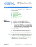
Graphs are given in the following where the number of real multiplications and additions/subtractions are given for FFT lengths of N = {8, 16, 32, 64, 128, 256, 512, 1024} in different scenarios of output pruning. The tested scenarios are listed below:
• M1: 50 % random output pruning
• M2: 50 % DSM output pruning where every upper node is chosen
• M3: 50 % DSM output pruning where every lower node is chosen
• M4: 50 % ASM output pruning where the upper half output is chosen
• M5: 50 % ASM output pruning where the lower half output is chosen
• M6: 20 % ASM output pruning where the upper half output is chosen
In the description of the scenarios the word ”chosen” means that the current node/output is
not pruned.
In fact seven scenarios is tested because the radix-2 and split-radix FFTs is also tested for
comparison. In the following figures: R2FFT = radix-2 FFT, SRFFT = split-radix FFT,
PR2FFT = pruned radix-2 FFT, PSRFFT = pruned split-radix FFT.
30
3.2 Computation Count
4
4
x 10
R2FFT
SRFFT
PR2FFT
PSRFFT
2
1.5
1
0.5
0
8
16
2.5
Number of multiplications
Number of multiplications
2.5
(a) Real multiplication count for 90 % random output pruned FFTs
R2FFT
SRFFT
PR2FFT
PSRFFT
2
1.5
1
0.5
0
32 64 128 256 512 1024
Number of inputs
x 10
8
16
32 64 128 256 512 1024
Number of inputs
(b) M1: Real multiplication count for 50 % random
output pruned FFTs
Figure 3.5: Number of real multiplications used in 90 % and 50 % random output pruned FFTs.
4
Number of add/sub
3
2.5
4
x 10
R2FFT
SRFFT
PR2FFT
PSRFFT
2
1.5
1
0.5
0
3.5
3
Number of add/sub
3.5
2.5
x 10
R2FFT
SRFFT
PR2FFT
PSRFFT
2
1.5
1
0.5
8
16
32 64 128 256 512 1024
Number of inputs
(a) Real addition/subtraction count for 90 % random output pruned FFTs
0
8
16
32 64 128 256 512 1024
Number of inputs
(b) M1: Real addition/subtraction count for 50 %
random output pruned FFTs
Figure 3.6: Number of real additions/subtractions used in 90 % and 50 % output pruned FFTs.
Figure 3.5(b) and 3.6(b) illustrate that the 50 % output pruned FFTs are close to their
non pruned counter parts. This is not the case for figure 3.5(a) and 3.6(a) where many
computations are saved by using the pruning algorithms. Furthermore the 50 % pruned radix2 FFT uses approximately 25 % more multiplications than the split-radix FFT.
31
Pruning FFT
4
4
x 10
R2FFT
SRFFT
PR2FFT
PSRFFT
2
1.5
1
0.5
0
8
16
2.5
Number of multiplications
Number of multiplications
2.5
(a) M2: Real multiplication count for 50 % DSM
output pruning where every upper node in the outputvector of M is chosen
R2FFT
SRFFT
PR2FFT
PSRFFT
2
1.5
1
0.5
0
32 64 128 256 512 1024
Number of inputs
x 10
8
16
32 64 128 256 512 1024
Number of inputs
(b) M3: Real multiplication count for 50 % DSM
output pruning where every lower node in the outputvector of M is chosen
Figure 3.7: Number of real multiplications used in 50 % DSM output pruned FFTs.
4
Number of add/sub
3
2.5
4
x 10
R2FFT
SRFFT
PR2FFT
PSRFFT
2
1.5
1
0.5
0
3.5
3
Number of add/sub
3.5
2.5
x 10
R2FFT
SRFFT
PR2FFT
PSRFFT
2
1.5
1
0.5
8
16
32 64 128 256 512 1024
Number of inputs
(a) M2: Real addition/subtraction count for 50 %
DSM output pruning where every upper node in the
outputvector of M is chosen
0
8
16
32 64 128 256 512 1024
Number of inputs
(b) M3: Real addition/subtraction count for 50 %
DSM output pruning where every lower node in the
outputvector of M is chosen
Figure 3.8: Number of real additions/subtractions used in 50 % DSM output pruned FFTs.
In figure 3.7 and 3.8 the worst case scenario for 50 % output pruning is shown. It is the worst
case because only nodes at the output are pruned when every second output or subcarrier is
chosen. In figure 3.7(b) nothing is gained by pruning the radix-2 FFT with 50 % because the
location of the twiddle factors is always placed at the lower right node in the butterfly, see figure
2.4. Furthermore the pruned radix-2 FFT exceeds the split-radix FFT with approximatly 25
% in the multiplication count.
32
3.2 Computation Count
4
4
x 10
R2FFT
SRFFT
PR2FFT
PSRFFT
2
1.5
1
0.5
0
8
16
2.5
Number of multiplications
Number of multiplications
2.5
(a) M4: Real multiplication count for 50 % ASM
output pruning where the upper half outputvector
of M is chosen
R2FFT
SRFFT
PR2FFT
PSRFFT
2
1.5
1
0.5
0
32 64 128 256 512 1024
Number of inputs
x 10
8
16
32 64 128 256 512 1024
Number of inputs
(b) M5: Real multiplication count for 50 % ASM
output pruning where the lower half outputvector
of M is chosen
Figure 3.9: Number of real multiplications used in 50 % ASM output pruned FFTs.
4
Number of add/sub
3
2.5
4
x 10
R2FFT
SRFFT
PR2FFT
PSRFFT
2
1.5
1
0.5
0
3.5
3
Number of add/sub
3.5
2.5
x 10
R2FFT
SRFFT
PR2FFT
PSRFFT
2
1.5
1
0.5
8
16
32 64 128 256 512 1024
Number of inputs
(a) M4: Real addition/subtraction count for 50 %
ASM output pruning where the upper half outputvector of M is chosen
0
8
16
32 64 128 256 512 1024
Number of inputs
(b) M5: Real addition/subtraction count for 50
% ASM output pruning where the lower half outputvector of M is chosen
Figure 3.10: Number of real additions/subtractions used in 50 % ASM output pruned FFTs.
Instead of pruning randomly at the output, ASM subcarrier allocation has been used in figure
3.9 and 3.10. In all four figures the pruned FFTs are less computionally demanding than their
non pruned counter parts. The pruned split-radix achieves the lowest multiplication count
and the radix-2 FFT is best in addition/subtraction count. This is because the additions/subtractions are only pruned in the case that twiddle factors are pruned, and the radix-2 FFT
has the most twiddle factors. It is also seen that the ASM for the upper half nodes achieves
the best results for the pruned FFTs compared to ASM with the lower half not pruned. This
is due to the structure of the flow graphs of the radix-2 and split-radix FFT where the most
twiddle factors are located at the ”bottom”, see figure 2.5 and 2.9.
33
Pruning FFT
4
4
x 10
R2FFT
SRFFT
PR2FFT
PSRFFT
2
1.5
1
0.5
0
8
16
2.5
Number of multiplications
Number of multiplications
2.5
(a) M1: Real multiplication count for 50 % random
output pruned FFTs
R2FFT
SRFFT
PR2FFT
PSRFFT
2
1.5
1
0.5
0
32 64 128 256 512 1024
Number of inputs
x 10
8
16
32 64 128 256 512 1024
Number of inputs
(b) M6: Real multiplication count for 20 % ASM
output pruning where the upper half outputvector
of M is chosen
Figure 3.11: Number of real multiplications used in 50 % random and 20 % ASM output pruned FFTs.
4
Number of add/sub
3
2.5
4
x 10
R2FFT
SRFFT
PR2FFT
PSRFFT
2
1.5
1
0.5
0
3.5
3
Number of add/sub
3.5
2.5
x 10
R2FFT
SRFFT
PR2FFT
PSRFFT
2
1.5
1
0.5
8
16
32 64 128 256 512 1024
Number of inputs
(a) M1: Real addition/subtraction count for 50 %
random output pruned FFTs
0
8
16
32 64 128 256 512 1024
Number of inputs
(b) M6: Real addition/subtraction count for 20 %
ASM output pruning where the upper half outputvector of M is chosen
Figure 3.12: Number of real additions/subtractions used in 50 % random and 20 % ASM output pruned
FFTs.
Figure 3.11 and 3.12 shows that subcarrier allocation is very important and that ASM output
pruning is superior to DSM output pruning. Approximately the same results are obtained with
50 % random output pruning compared to only 20 % ASM output pruning. In [22] Sorensen
and Burrus compare different pruning FFTs with the split-radix FFT with the respect to
number of computations. They show that with approximately 90 % pruning and an FFT
length of 512 the computations of the pruned FFTs begin to exceed the split-radix FFT.
However it has just been shown that if the outputs are chosen correctly, both the pruned
radix-2 and split-radix FFT with 50 % ASM output pruning requires less computations than
the split-radix FFT.
34
3.2 Computation Count
In summary this chapter has presented some interesting results and given subjects for further
analysis in the hardware implementation. An analysis was made of the number of computations
used by the radix-2 FFT, split-radix FFT and their pruned counterparts. It was shown that the
pruned split-radix FFT was superior to the others in using the least number of computations
in the six scenarios developed and tested in Matlab. An algorithm for pruning the split-radix
FFT at the output has been proposed together with an algorithm for counting the number of
computations used by the pruned radix-2 and the split-radix FFT. There are no restriction
on the number of outputs when pruning the FFTs. Furthermore the computation count of
the algorithms shows that ASM subcarrier pruning is superior to DSM pruning and is highly
effective.
The survey of the pruning FFTs showed an interesting topic which should be analysed in
the hardware implementation. Sorensen stated in [22] that the cost with regards to speed
of performing a conditional statement exceeds the savings of performing a single complex
addition in sequential computing. In hardware it will be discussed if additions can be pruned
as well.
Based on this survey the pruned split-radix FFT and the split-radix FFT will be analysed
for further implementation and comparison. First the available hardware and software is
described, followed by a summary and the problem statement.
35
Pruning FFT
36
4
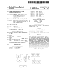
Available HW/SW
The purpose of this chapter is to describe the hardware platform and software tools, which
can be used to implement the split-radix FFT and the pruned split-radix FFT algorithms.
First a hardware platform is chosen. The group has chosen to use the Altera DE2 board, which
contains a Cyclone II Field Programmable Gate Array (FPGA). Then the software tools, which
match the hardware platform, and the possibilities and limitations they impose on the solution
are described. The used tools are part of the Quartus II Software Suite developed by Altera.
Finally three different implementation methods are chosen. The first solution is to implement
a softcore processor on the board and then execute the algorithm implemented in C code. The
next solution is to hardware accelerate parts of the C code, executing on the FPGA. The last
solution is a pure hardware implementation of the algorithm.
4.1
Available Hardware
In this section the hardware available to the project group is described. The FPGA was chosen
as the main development platform because of the following reasons:
• Possibility to make parallel computations.
• Easy and fast reconfiguration of the FPGA.
• Flexibility. It is possible to add and design many different functions on the FPGA.
• From an educational point of view the FPGA is interesting, since the group has never
worked with such a device before.
The FPGA also has some limitations e.g. number of resources (memory, logic elements)
and performance (as compared to a highly specialized Application-Specific Integrated Circuit
(ASIC)). In this project these limitations do not give rise to any problems, since the algorithm
37
Available HW/SW
is not memory demanding and furthermore the performance of the FPGA does not affect the
comparison between the different solutions.
In the following the basics of an FPGA are explained. Finally the features of the selected
development board and the FPGA, located on the specific board, are described.
Basic FPGA design
The description of the FPGA design is based on a lecture given by Yannick Le Moullec, [18].
An FPGA consists of a huge amount (100.000 v 3.000.000) of logic elements. These logic
elements can be used to implement the functionality of e.g. an adder or a multiplier. The idea
with the FPGA is that the logic elements can be interconnected in various ways to perform a
task specified by the developer.
Basically there are three different FPGA architectures: island, hierarchical and logarithmic.
All three architectures are used to establish connections between logic elements, memory, and
in- and outputs. According to [18] the logic elements are based on two different setups, either
a look-up table and a flipflop or a combination of multiplexers.
The island architecture is based on a large grid network on which configurable elements are
placed. The elements connect to the grid via connection blocks, which either are connected to
a horizontal or vertical set of lines in the grid. The horizontal and vertical lines are connected
in an interconnection matrix. This architecture is used by Xilinx.
The hierarchical type is a level based approach. The lowest level contains logic elements,
memory blocks, and connections. The next level consists of several blocks from the lowest
level and so forth. Altera uses this architecture and in their design the lowest level is made up
of logic elements. The next level is based on Logic Array Blocks (LABs), which each contain
16 logic elements. In some Altera FPGAs there is a third and final level, which consist of
MegaLABs that each contain 16-24 LABs. The in- and outputs are connected to the interconnection busses on the LAB or MegaLAB level.
The last architecture type is the logarithmic. It is also a hierarchical type, but the difference
is that the number of elements is based on the current level. That is on the i’th level the
number of elements is equal to 42·i .
Some FPGAs also contain elements, which are embedded e.g. multipliers or even a full processor core. In Simulink these hardwired components can be selected by clicking the option
”use dedicated hardware” in the current block. If for example an embedded multiplier has
to be used in an implementation based on compilation of e.g. C code, the developer has to
change the produced hardware description language (HDL). In stead of using the multiplier
generated by the compiler and written in HDL the developer can change the code so that the
embedded multiplier is utilized in the given function.
This was a brief overview of the FPGA and its architecture. In the next section the selected
development board and the matching FPGA are descriped.
The development board
The group has several boards at its disposal in the laboratory, but the Altera DE2 Development
and Education Board is the only board which may be used in the group room and furthermore
it is supported in Simulink (see section 4.2), which the DE1 board is not. Therefore the Altera
DE2 was chosen as the platform for the implementations.
The description of the board is based on [4].
38
4.1 Available Hardware
The board is designed around the Cyclone II 2C35 FPGA, [6]. On the boards used by the group
the FPGA is version EP2C35F672C6N. Figure 4.1 illustrates the DE2 board, the components
on the board and the in- and outputs.
Figure 4.1: The DE2 board and the in- and outputs. [4, Figure 2.2].
The components, which are important in this project are:
• The Cyclone II FPGA.
• The USB Blaster, which is used to establish a connection between the board and a PC.
• The standard 50 MHz clock.
• RAM.
The main unit on the DE2 board, the Cyclone II FPGA comes in many editions. The 2C35
has:
• 33126 Logic Elements.
• 105 M4K dual-port RAM blocks, which consist of 4 kilobits. The data width is up to
36 bits. In total 483840 RAM bit available.
• 35 18x18 bit embedded multipliers.
• 4 phase-locked loops.
• 475 user in- and output pins.
In this section the available hardware was described. The used development platform is an
Altera DE2 board, which utilizes a Altera Cyclone II FPGA. In the following section the
available software tools are described. The tools are used, when the developer wants to design,
implement, simulate and run software for the FPGA.
39
Available HW/SW
4.2
Available Software
In this section the available software tools, which can be used to implement the algorithm on
the Altera DE2 board, are described. The tools are located in the Altera Quartus II Software
Suite.
In figure 4.2 the different tools and their interconnections are illustrated. The figure is made
so that the top illustrates the high level Matlab and C code software, and in the bottom the
low level with the Cyclone II FPGA is shown.
Matlab/ C Code
Simulink
(Matlab)
Manual transcription
IDE Nios II
DSP
Builder
Hardware description languages:
VHDL/Verilog/Handel-C
SOPC
Builder
C2H
Accelerator
Quartus:
Compiler HDL
Communication with the board
Nios II
FPGA Cyclone 2
Figure 4.2: The available tools for implementation of the algorithms on the DE2 board.
As can be seen from the figure there are many ways in which the split-radix FFT algorithms
can be implemented. In the following the different possibilities are described:
• One option is to manually convert all the C code into a Hardware Description Language
(HDL). The platform Quartus is then used to compile the HDL code and send the
produced binary file to the board. Quartus can compile VHDL, Verilog, and HandleC. The main advantage of this approach, is the possibility to work in a low level of
abstraction. It makes it possible to highly optimize the architecture, with regards to
parallelism and the used number of bits for variables. The drawback is that the project
group has to learn a new description language, which will require a lot of time.
40
4.2 Available Software
• Another option is to use the DSP Builder provided by Altera, which is a block library
plugin to Simulink provided by Matlab. Simulink is a graphic block diagram program,
which can be used to model and simulate designs. Furthermore the program is interconnected with Matlab, which means that variables can be downloaded and uploaded from
the program to the Matlab workspace.
The DSP Builder is available in the Altera Quartus II Software Suite. The DSP Builder
contains a set of special blocks for the Altera DE2 board. There are many advantages using this approach. Simulink is a subsystem of Matlab, which is well known by the group.
It is a graphical block diagramming tool, so it is more user friendly than HDL. Another
point is that when compiling and building the project, Simulink is calling the necessary
tools from Quartus without the need of having this program running. The main problem using the DSP Builder is that it is made for data flow and it is not very suited to
manage control flow. Moreover the DSP Builder miss a lot of building blocks that only
Simulink is providing. Sufficient data sheets specially concerning delays introduced by
each building block are also missing.
The two above described design flows are hardware oriented. The level of abstraction is very
low for the first solution, but for the latter one the level is closer to a system-level, because
the user can insert e.g. an adder block in stead of writing the code for the function.
• A third way is to use a software design flow using the softcore Nios II processor and the
Integrated Development Environment(IDE) Nios II, which belongs to the Nios II Embedded Design Suite. The Nios II is a processor developed by Altera and supported by
the Cyclone II FPGA. It is configurable that is the designer can make his own internal
peripherals or use the set proposed by Altera. The interface of the IDE is based on
Eclipse, which is an open source IDE.
The IDE Nios II is used to compile the C code and send it to the Nios II softcore on
the DE2 board. This process requires different tools. The Quartus and the system-ona-programmable-chip (SOPC) Builder are used to build the Nios project. The SOPC
Builder is made for managing the architecture of the Nios II processor system with a
graphical block interface. Quartus is used to compile the code end send it to the board.
This approach has several advantages. With regards to the time-to-market, according to
Altera, this design suite is very good, allowing the designer to focus on the architecture
and raising the level of abstraction. The groups experience of this time-to-market claim
will be evaluated later after the implementation has been made. With regards to the
purpose of the implementation, a good thing is that many configurations of the Nios II
processor system are available, making it possible to omit its complex configuration.
The Hardware Abstraction Layer (HAL) Application Programming Interface (API), provides useful C functions. The HAL API is located in the Quartus II Software Suite. For
example it has a function for measuring the execution time on the Nios II processor. The
groups first impression is that the main drawbacks are the complex tools, the IDE, the
Quartus and the SOPC. It takes a long time to learn them, and to be able to perform
very simple examples. The way they communicate is often not transparent to the user
which makes the understanding, the debugging, and the optimization of the mechanisms
difficult.
The above described design method is oriented towards a full software implementation. However the combination of the tools introduces the possibility to make a hardware/software
(HW/SW) codesign flow. There are two main ways to do this:
41
Available HW/SW
• The C-to-Hardware (C2H) compiler can accelerate chosen parts of the C code into HDL
code. This tool is available in the IDE Nios II, and according to Altera this should not be
a difficult approach for the user. To accelerate functions the IDE uses SOPC builder and
Quartus. The drawback is that the mechanisms behind the C2H are not well described
in the documentation provided by Altera.
• The second way assigns the HW/SW codesign approach to the designer. The designer
can make the data path with HDL or Simulink, and then use the Nios II to compile
the C code for the control path. Therefore issues of interconnection between both parts
have to be managed. This approach is very flexible, because the designer could choose
the level of abstraction for each part of the device.
To conclude this overview of available tools, the group has decided for two implementation
approaches. The first approach is a full hardware solution using the DSP Builder in Simulink.
This tool is very user friendly which leads to a straight forward implementation, without
spending time to learn a new tool. Furthermore it gives the opportunity to have full control
of the data and control path. The second approach is to use the IDE Nios II. The first step is
to do a full software implementation, and in the second step to use the C2H compiler. This
approach is supported by the fact that the HW/SW codesign is achievable in a relative short
time, which gives the first measurements of an implementation.
In the next chapter the work presented so far in the report is summarized and the goals
for the implementations are set up.
42
5
Problem Statement
This chapter contains the problem statement, which forms the basis for the analysis performed
on the split-radix FFT algorithms implemented on the DE2 board. To support the problem
statement, the choices made by the group in the previous chapters are summarized in this
chapter.
The initiating problem in section 1.1 delt with the comparison between the normal and pruning FFT under different ASM and DSM scenarios. The analysis was limited to having no
focus on channel conditions. Furthermore the analysis was restricted to one time slot which
entails that the system do not need to adapt to changing subcarriers.
The performance and complexity was defined in section 1.2. Performance was restricted to
execution time and resource usage. Complexity which affects the performance was defined as
the number of computations and control structures used by the pruning FFT. In chapter 2
three different FFT algorithms were presented. Based on results submitted in different articles
the split-radix FFT was selected in favour of the radix-2 and radix-4 algorithms. Using a C
code given in Skodras article [21] a split-radix FFT was implemented in Matlab. Next the
algorithm was modified, to enable it to prune the output. Furthermore the radix-2 algorithm
was also pruned, to ensure that the pruned split-radix could be compared with another pruned
FFT. The modifications made on the algorithms were presented in chapter 3. In this chapter
computation counts of the required number of real multiplications and real additions/subtractions were measured in Matlab. The computation tests were made on six different pruning
scenarios. The results obtained showed that the pruned split-radix is the cheapest algorithm
with regards to the required computations and therefore it was selected for analysis and implementation in hardware.
To make the implementation the available hardware platforms and software tools were analysed in chapter 4. The group chose the Altera Development and Education Board (DE2)
containing an Altera Cyclone II FPGA as the hardware platform. This lead to the choice of
Alteras Quartus II as the main IDE.
As described in chapter 4 there are many different approaches to perform the implementa43
Problem Statement
tion in hardware. It was chosen to make a high level software implementation on the Nios II
softcore and a system level hardware implementation with the DSP Builder Simulink toolbox.
Furthermore a hardware-software codesign by use of the Nios II C2H accelerator was chosen.
The further analysis
Based on the selection of the pruned split-radix FFT algorithm and the two main design approaches the problem statement is made. The goal with the implementation is to analyse if
the pruned split-radix FFT is applicable from a time wise point of view. That is the analysis
should determine whether or not it is possible to save computation time by using the pruning
implementation. Furthermore the difference in hardware resource usage between the pruned
and non-pruned split-radix implementation will be examined.
When the time measurements are finished the results will be compared with the computation
counts from Matlab to check for consistency that is: does a low complexity count in Matlab
equal a fast calculation on the DE2 board?
As already mentioned that due to the limited project time the group has decided not to
generate and update a matrix M, containing the ”pruning locations”. This means the implementations only perform one FFT on one sample (containing 1024 values) and with a
preloaded pruning matrix. If the matrix is to be changed the implementations will have to be
recompiled with the new matrix.
In the following chapters the three implementations are described. The chapters are structured so that the first section of the chapter describes the design of the implementation. Then
the implementation itself is described. When the solution has been implemented the time and
resource tests are performed and the results are written in the third section of the chapter.
Finally the results are discussed and suggestions for further development are given.
44
Part III
Design, Implementation and Test
45
6
SW and HW/SW Solution
The objective of this chapter is to compare the performance of the split-radix FFT and the
pruning split-radix FFT algorithms with regards to execution time. The algorithms, will as
stated in chapter 4, be implemented and analysed based on a SW and a HW/SW solution. The
following sections will describe the design and implementation of the two solutions followed by
tests of the implementations. The tests will be made with the seven scenarios developed and
tested in Matlab, see page 31 - 34. The resource usage is not tested in the SW and HW/SW
implementations.
The result of the tests is that the implemented SW and HW/SW solutions work. The generated
outputs are equal to the split-radix FFT outputs from Matlab. The problem is that it has
not been possible to measure a consistent and repeatable execution time for the two solutions.
Several measurement methods and implementations have been made but the execution time
results are still not reliable.
6.1
Design
The design of the split-radix and pruning split-radix FFT algorithms used in the SW solution
is the same as the design used in the algorithms in section 2.4 and 3.1, respectively. The
algorithms are written in C, and they are based on the code given in [21]. The design of the
HW/SW solution is a successor to the SW solution. This section will deal with the design of
SW and HW/SW solution and with the changes, which were applied to the C code to make
it possible to accelerate certain functions into HW.
The design consists of three parts. First a profiling of the C code must be performed to
analyse which functions should be accelerated into HW. The next part deals with the fact
that the functions implemented in HW does not support floating-points, and therefore the
inputs have to be converted to a fixed-point representation. When the code has been profiled
and converted to fixed-point the design flow used for the implementation on the Altera DE2
board is presented.
47
SW and HW/SW Solution
Profiling the code in Matlab
The profiling of the code has been made in Matlab. The reason why it is possible to perform
the profiling in Matlab and not directly on the C code is because the transformation of the
C code into Matlab code (presented in chapter 2 section 2.3) has been made one-to-one.
Furthermore the profiling tool in Matlab is available and easy to use.
The results of the profiling are shown in figure 6.1 and 6.2. The number in the left most
column represents the time (in seconds) spent at that given line in the code. The time
measurement is specific for the platform where the profiling is made, but the trends indicated
by the measurements are considered to be the same on most platforms. The next column
represents the number of times that line has been called. The column to the left of the code
is the line number. The dark red marking of the code indicates that the current line is more
time consuming than the lines with white markings.
Figure 6.1: The output of the Matlab profiling of the first part of the split-radix FFT algorithm.
48
6.1 Design
Figure 6.2: The output of the Matlab profiling of the last stage of the spilt-radix FFT algorithm.
The absolute time measurement is not reliable due to the memory cache in Matlab. When the
profiler is used several times the value of the time measurement actually decrease. However
the profiler always indicates the most time consuming lines, and these remain the same during
all tests.
The most time consuming lines for the first profiling are in the innermost loop, and they are
due to the arithmetic operations performed here. These lines correspond to line 23-43 in figure
6.1. The latter profiling shows that a lot of time is used in the last stage butterflies shown in
figure 6.2, lines 56-63. Based on the profiling it is decided to export the innermost loop and the
last stage butterflies into two other functions, so that they can be optimized by implementing
them in hardware.
Conversion from floating-point to fixed-point
The used Nios II processor system has a 32 bit architecture that supports floating-point.
The problem is that the accelerated HW implementation does not. Documentation for the
maximum word length in the accelerated HW has not been easy to find. It is therefore assumed
that the maximum word length is a 32 bit fixed-point word and that the data type is set to
integers.
To perform the conversion of the variables a manual scaling and round off the input data
(which is between -1 and 1) is used. This is also done for the cosines and sines used in the
algorithm. To ensure that the scaling and rounding is working correctly the output of the
algorithms have to be compared with the Matlab results, when the implementation is made.
The approach for the conversion of cosines and sines is shown in figure 6.3.
49
SW and HW/SW Solution
Double - Floating point
Cos/Sin
Scaling
*1024
Long Integer - Fixed point
Type Casting
HW
Butterfly()
Cos/Sin
Type
Uncasting
Double -Floating point
Unscaling
>>10
Long Integer - Fixed point
Long Integer - Fixed point
Figure 6.3: The method used for transforming floating-points into fixed-points.
In this implementation the accuracy of the output is not the main goal. The accuracy should
only be high enough to verify that the implementation has been made correctly. Therefore
the scaling factor is set to 10 bits that is the values are multiplied with 210 . The cosines and
sines are between -1 and 1 so a scaling with 231 could have been made for optimizing the
precision. The round off is done by making a C type cast from double into a long integer.
The word length of a long is 32 bits. To unscale the output, a shift operation is used instead
of a division, because it is less expensive to perform. The solution used for the conversion is
very expensive with regards to number of operations, because one multiplication has to be
used for each cosine and sine value. The aim of this implementation is however to compare
the pruning algorithm with the non pruning one, and since the scaling is identical for both
implementations it does not affect the results.
The conversion into fixed-points will introduce a small error when comparing the final outputs from the split-radix FFT with the outputs obtained in Matlab. The introduced error is
caused by two factors: 1) the type casting of the cosines and sines and 2) the type casting
of the inputs. The inputs, generated in Matlab, are random base 10 numbers with 5 digits
before and 1 digit after the radix point. The absolute maximum value of the numbers within
the algorithm is tested to be approximately 7 · 105 . The inputs are rounded but not scaled.
Design Flow
After the C code has been profiled and the variables have been scaled, the code is ready
for the SW and HW/SW implementation. A sketch of the code with the hardware accelerated functions is illustrated in figure 6.4. A detailed flow diagram is given in the following
Implementation section in figure 6.9.
50
6.1 Design
Start SRFFT
The
three
loops
Last
stage
loops
Done
Butterfly()
(HW accelerated)
Finish SRFFT
LastStageButterfly()
(HW accelerated)
Figure 6.4: Sketch of the C code with the chosen functions in HW.
The design is made for the Altera DE2 board, which was selected in chapter 4. The design flow
when using the Quartus II Software Suite is presented next. The design is based on [11] and
[12]. The design flow can be divided into two parts. First the creation of a processor system,
which is to be run on the Cyclone II FPGA. Next the Integrated Development Environment
(IDE) Nios II is used to handle the C code and the compilation of it. The IDE Nios II is also
used to select the functions which will be accelerated into HW with the C-to-Hardware (C2H)
compiler. The first part of the design flow is illustrated in figure 6.5.
Creation of Nios II
processor
SOPC Builder
HDL
Compilation and
download to board
Quartus II
.sof
SRAM
DE2 board
Figure 6.5: The design flow for the creation of a processor system on the Cyclone II FPGA.
First the processor system is created in the SOPC Builder. The program is a graphical user
interface used for the creation of a system or a ”minicomputer”, where each required system
component can be added. The output of the SOPC Builder is a specified HDL file which can
be compiled by the Quartus II. The output of Quartus II is a SRAM Object File (.sof) which
is then uploaded in the SRAM on the Altera DE2 board.
A processor system handling the C code must therefore be designed for the Cyclone II FPGA
on the Altera DE2 board. For simplicity the design of the processor system is a Nios II processor system based on the Nios II core. The information about the Nios II processor system
and the Nios II core is based on [8] and [10], respectively.
A standard demonstration of a Nios II processor system has been used. The project is named
DE2_NIOS_DEVICE_LED and is available at [25] (also placed on the enclosed CD of the report).
This approach is used because creation of a processor system is not the main scope of the
project. In the following section the main components of the processor system are described.
In figure 6.6 the Nios II processor system from DE2_NIOS_DEVICE_LED is shown.
51
SW and HW/SW Solution
Clock
Reset
JTAG connection
to software debugger
JTAG Debug
Module
Nios II Processor System
UART
Data
Nios II
Processor Core
SDRAM
Memory
Timer 0
Timer 1
SDRAM
Controller
Flash
Memory
Tristate bridge to
off-chip memory
Avalon Switch Fabric
On-Chip SRAM
SRAM
Memory
Instr.
TXD
RXD
LCD Display
Driver
LCD Screen
General-Purpose
I/O
Buttons,
LEDSs etc.
CompactFlash
Interface
SD Card
AUDIO DAC
Amplifier
VGA Controller
VGA Monitor
EPCS16 Config.
Interface
Amplifier
Figure 6.6: The Nios II processor system in the project DE2 NIOS DEVICE LED. The amplifiers
and the VGA monitor are examples of equipment that could be connected to the system. Made with
inspiration from [8].
The fundamental component of the system is the Nios II processor core. Three standard cores
come with the Quartus II software: economic, standard, and fast. The objective with the
design of the economic core is its small area with the cost of speed. Its maximum number of
million iterations per second (MIPS) is 31. The standard core is said by Altera to be the best
trade off between area and speed with a MIPS of 165. The fast core provides a maximum of
218 MIPS with up to 1800 logic elements. The economic core only provides up to 700 logic
elements. The project DE2_NIOS_DEVICE_LED uses the fast core (Nios II/f) which is shown in
figure 6.7. The default choice of the Nios II/f core has not been changed, because the resource
usage is not tested for the SW and HW/SW implementations.
52
6.1 Design
JTAG connection
to software debugger
JTAG
Debug
Module
Nios II Processor Core
Tightly Coupled
Instr. Memory
Reset
Clock
CPU Resetrequest
CPU Resettaken
IRQ [31 … 0]
General
Purpose
Registers
R0 to r31
Program
Controller
&
Address
Generation
Exception
Controller
Interrupt
Controller
Instruction
Cache
Control
Registers
Ctl1 to ctl15
Tightly Coupled
Instr. Memory
Instr. Bus
Data Bus
Tightly Coupled
Data Memory
Aritmetic
Logic Unit
Data
Cache
Tightly Coupled
Instr. Memory
Figure 6.7: The Nios II/f processor core used in the project DE2 NIOS DEVICE LED [11, p. 2-2].
In DE2_NIOS_DEVICE_LED the maximum frequency of the core is set to 100 MHz which results
in 101 MIPS. According to the specification the number of MIPS could be increased but with
the risk that the scheduling with internal and external peripherals would cause errors. Therefore the frequency has not been changed. At the current frequency the core uses 1400 - 1800
logic elements. The Nios II/f provides embedded multipliers in hardware for increasing the
speed. The ALU uses 35 embedded 32 bit × 16 bit multipliers. Another option is to use 32
bit × 4 bit multipliers implemented by logic elements. For further improvement of the speed
the Nios II/f core is designed with a separate data and instruction cache instead of using the
peripheral memory (SDRAM). The data cache is set to 2 kB and the instruction cache to 4 kB.
To enable the use of debugging tools the JTAG debug module is enabled. It allows the
designer to e.g set SW breakpoints. Under the design and implementation phase of the system it is also used for downloading the C code, created in the IDE Nios II, to the board.
Furthermore it is used to feedback results from the board to the PC.
The design of the processor system has now been described and it is ready for processing
the C code. The IDE Nios II is used for handling the C code and the acceleration of the
chosen function into HW with the use of the C2H compiler. Hereafter the code is sent to the
board. This is illustrated in figure 6.8. The builder of the C code is set not to optimize the
code.
53
SW and HW/SW Solution
PC
C code
Board
JTAG
IDE Nios II
Process data
PC
JTAG
Nios II processor system
Send results to PC
IDE Nios II
Figure 6.8: The flow of how the C code is executed on the Altera DE2 board.
The C code for the SW implementation is created in the IDE Nios II. Hereafter it is sent
through the JTAG connection to the Nios II/f core. The data is processed and sent back to
the IDE Nios II. The output data can then be compared with the implementation in Matlab.
The same approach is used for the HW/SW solution. The C2H uses the SOPC Builder
to accelerate the chosen functions and to generate the interface with the processor system on
the board. The output from the SOPC Builder is compiled by Quartus II and uploaded to the
SRAM. The C2H compiler recognizes events that can occur in parallel. Arithmetic operations
such as additions and multiplications become a direct one-to-one mapping in hardware, where
the sharing of the accelerated arithmetic units depends on the degree of parallelism, [9].
6.2
Implementation
The SW and the HW/SW implementations on the DE2 board are described in the following
section. A detailed flow graph of the code representing both implementations is shown in
figure 6.9. The difference between the two implementations is that the specified functions
from the Design section, 6.1, will be accelerated into HW for the SW/HW implementation.
54
6.2 Implementation
Start SRFFT
k=1
Initialize
n2, n4, L, and ip1
k≤ m-1
No
Yes
Initialize is and id
Update e and a
ia = 1
j=1
ia ≤
m +1
No
2
j ≤ n4
Finish
is = id * 2 – 1
id = id * 4
L = (L + 2) / 4
i0 = 1
ib ≤ L
Yes
j=j+1
LastStageButterfly()
(HW accelerated)
n2 = n2 / 2
n4 = n4 / 2
ip1 = ip2
Calculate cosine
and sine
ib = 1
No
No
Yes
Yes
ia = ia +1
k = k +1
No
i0 ≤
nob[k]
Yes
i0 = i0 + 1
Butterfly()
(HW accelerated)
i0 = i0 + 1
Figure 6.9: Flow graph of the C code with the chosen functions accelerated in HW.
The SW implementation
The SW implementation is made in the IDE Nios II as described in the Design section. A
floating-point and a fixed-point version of the C code has been made to compare the execution
time.
When the C code is build in the IDE Nios II, the code is run by loading the code to the Nios II
core/f through the JTAG Debug connection, as illustrated in figure 6.8. In the main function
of the C code it is specified that the output data is printed to the terminal of the IDE Nios
II via the stdout variable. The printing is made with the printf() function. The outputs x
and y (real and imaginary outputs, respectively) are then compared with the results obtained
in Matlab.
55
SW and HW/SW Solution
The HW/SW implementation
To accelerate the two functions, specified in the design section, the C2H compiler is called in
the IDE Nios II. The C2H compiler makes a hardware block, which substitutes the C function
and the wrapper between the generated HW block and the C code. As mentioned earlier the
inside of the innermost loop and the last stage butterfly functions are accelerated. The two
new HW blocks are then visible in the SOPC builder, and a synthesises report of the build
project is available in the IDE Nios II. In the synthesis report it is suggested that the loops as
well are accelerated into HW. The amount of used resources can also be read. The last step is
to reprogram the DE2 board with Quartus II, and to execute the C code. The implementation
flow can be seen in figure 6.10. The Nios II processor system is made before as illustrated in
figure 6.5.
C wrapper function
C2H Compiler
Specified C function
Analysing specified C
function
Build the HW based on
the function
IDE Nios II
C2H Compiler
C2H Compiler
Connection to existing
Nios II Processor and
creation of new Nios II
System
Compilation and
download to board
SRAM
SOPC Builder
Quartus II
DE2 board
Figure 6.10: The acceleration of a specified C function into HW using the C2H compiler.
6.3
Test
In this section the testing of the software implementations is described. The implementations
are: A floating-point pruning split-radix FFT, a fixed-point pruning split-radix FFT and a
C2H accelerated fixed-point pruning split-radix FFT. The implementations are compared with
an implemented floating- and fixed-point split-radix FFT.
First a test is made to check if the functionality of the algorithm is correct. Finally a test
is made to determine the execution time of the implementations. The test is made with the
different scenarios, which were used in the Matlab implementation, see page 31 - 34. During
the execution time test the group determined that the results are not reliable. Therefore three
other implementations and two other time measurement tools were used to try to achieve
coherent results. The main ideas with the other implementations and tools are explained after
the first test results are presented.
The functionality check was made by comparing the outputs of the fixed-point and the
HW/SW implementations with the floating-point implementation. The values of the floatingpoint implementation are known to be correct, because the implementation is based on Skodras
et al.s algorithm presented in [21], which has been verified in Matlab. The objective is that
56
6.3 Test
the difference between the values should be small enough for the group to conclude that the
values are the same. If the values are the same it proves that the implementation is performing
the split-radix FFT.
The results of the tests were similar, and they both confirmed that the implementations work,
and therefore only one of them is explained in this section. The result of the comparison
between the fixed-point and the floating-point is that the mean error is only 0,16%. This is
illustrated in figure 6.11. The test is performed with a 1024 point FFT.
x error
1
0.8
0.8
0.7
0.7
0.6
0.6
0.5
0.4
0.5
0.4
0.3
0.3
0.2
0.2
0.1
0.1
0
0
200
400
600
1024 values
800
1000
Y error
Y mean error
0.9
y error in %
x error in %
0.9
y error
1
X error
X mean error
0
0
200
400
600
1024 values
800
1000
Figure 6.11: Result of the comparison between fixed-point and floating-point. The error function is
the subtraction between the fixed-point output and the floating-point output. The variables x and y
are the real and imaginary outputs, respectively..
The first implementation used C functions to measure the execution time. These functions
are provided by the HAL API and they depend on the two timer devices [12, p. 6-11]:
• System Clock Driver
• Timestamp Driver.
The System clock Driver provides a function, alt_nticks(), which gives the number of clock
ticks since the last reset of the system. By setting a variable with the function in the beginning
of the code and one in the end, it is possible to determine the number of ticks the code takes.
By using the function alt_ticks_per_second(), which provides the number of ticks per
second, the number can be translated into time (in seconds). A complete description of the
test is given in section F.1 in appendix F.
In table 6.1 the measurements of the execution time is given for the SW and HW/SW solution.
The test is described in section F.1 and F.2 in appendix F.
57
SW and HW/SW Solution
Scenario
SRFFT
M0
M1
M2
M3
M4
M5
M6
SW floating point
solution [ms]
6535
6825
6752
6798
6799
6290
6387
6671
SW fixed point
solution [ms]
3638
3553
3553
3553
3554
3545
3549
3553
HW/SW
solution [ms]
3728
3729
3729
3729
3729
3729
3729
3729
Table 6.1: Results of the measurement of the execution time in ms.
The different scenarios, M0-M6 are the ones which also where used in the computational count
in Matlab. For convenience they are repeated:
• M0: The split-radix FFT (no pruning), but with if sentences
• M1: 50 % random output pruning
• M2: 50 % DSM output pruning with every second upper node chosen
• M3: 50 % DSM output pruning with every second lower node chosen
• M4: 50 % ASM output pruning with the upper half output is chosen
• M5: 50 % ASM output pruning with the lower half output is chosen
• M6: 20 % ASM output pruning with the upper half output chosen
During the tests and afterwards the group noticed three major problems with the test. The
first one is that between two batches of tests of the same code, the results could change almost
30%, even using exactly the same code. Secondly the time measurement results also change if
some independent code is changed. Independent code is code, which is executed before or after
the two alt_nticks() variables are set. This is e.g. be printing of the output values at the
end of the C code. The third problem is that the non-pruning split-radix FFT, is slower than
the pruning one with the scenario M0 for the fixed-point implementation. This is a problem
since scenario M0 is equal to 0 % output pruning that is all ”if” structures (see listing 3.3 for
the code) in the code are true. Basicly this means that it is faster to execute a code which
contains a true ”if” structure as compared to a code without the structure. Based on these
observations the group concluded that the results are inconsistent, unrepeatable and therefore
not reliable.
It was however noticed that the difference between the different scenarios is stable, in the way
that over many batches of tests the results only change about 1%. The scenarios M4, M5 are
always the fastest, because the number of computations are decreased by 50% as compared
to the M0 scenario. Furthermore the implementation, which uses the C2H compiler, is slower
than the fixed-point implementation. This might be due to the fact that the time lost in
the communication between the Nios II and the hardware block, or access to the SDRAM,
is larger than the gain achieved by accelerating the functions into HW. The execution time
increases approximatively with 4.7 % from the fixed-point implementation to the HW/SW
58
6.3 Test
implementation.
To get reliable test results other time measurement tools were therefore examined. The reason
why the time measuring C function was exchanged, is because the function uses the system
clock timer, which might be interrupted. According to Altera the timestamp driver, mentioned
earlier, is more accurate. Therefore the tests where repeated with this function. Unfortunately
the achieved results are almost the same.
The second solution is to use the Performance Counter Core (PCC), [13]. This is a profiler
provided by Altera. To use the PCC a module called Performance Counter Unit has to be
inserted in the processor system by the SOPC Builder. This profiler makes it possible to measure the execution time over different sections, defined by the designer. In this project only
one is needed, and the output of the PCC is given in clock cycles and in seconds. The results
achieved with this second tool are better than before, because between different batches of
tests the result are almost the same. The changes in execution time between two consecutive
runs is now less than 2 milliseconds. Therefore the time measurements are believed to be
reliable.
There is however still a problem because the non pruning FFT is slower than the pruning FFT
using scenario M0. One reason to this problem, might be interrupts during the execution, due
to communication between the computer and the board through the debugger. Another source
might be the many unused modules in the Nios II project DE2_NIOS_DEVICE_LED.
Based on these assumptions the group has developed 3 implementations which are aimed at
solving the problems. The idea is to remove as many error sources as possible. In the execution
time tests of the following implementations the PCC is used. The three implementations are:
• Stand alone device
• Without cache
• The smallest architecture
First the stand alone implementation is made. In the IDE Nios II, the stdout is changed.
stdout is the block the C code sends the output of e.g. a prinft() to. The stdout is changed so
that the values are sent to the lcd screen on the Altera DE2 board. When the C code has been
built, the Flash Programmer is used in the IDE, to send the binary file, containing the code,
to the flash memory on the board. When the Nios II is reset it will run the program from the
flash memory and the result of the time measurement is printed on the lcd screen. The Nios
II can be manually resetted with the buttom Key0 on the board. This implementation and
test were made to test if the communication between the PC an the board causes problems.
Therefore only two scenarios are run: the non pruning split-radix FFT and the pruning splitradix FFT using the M0 scenario. The result achieved with this test shows the same tendencies
as the previous tests and therefore it is concluded that the problem does not come from the
communication between the PC and the board.
The next modification which the group made was to remove the instruction and data cache
from the Nios II processor system. This was made using the economic version called Nios II/e.
The implementation is illustrated in figure 6.12.
59
SW and HW/SW Solution
JTAG connection
to software debugger
JTAG
Debug
Module
Reset
Clock
CPU Resetrequest
CPU Resettaken
IRQ [31 … 0]
Program
Controller
&
Address
Generation
Exception
Controller
Interrupt
Controller
Nios II Processor Core
General
Purpose
Registers
R0 to r31
Instr. Bus
Control
Registers
Ctl1 to
ctl15
Data Bus
Aritmetic
Logic Unit
Figure 6.12: The NiosII/e, which is the smallest processor without instruction and data cache.
The cache was expected to cause problems, but the results were still not reliable because the
problem with the non-pruning FFT being slower persisted to exist.
The last implementation the group made was a very primitive Nios II processor system. The
following changes were made to the architecture using the SOPC Builder:
• The CPU is changed to the Nios II/e, which is the economic version. It is without:
– Data cache.
– Instruction cache.
– Hardware embedded multipliers.
• The only memory which is kept is the SDRAM.
• The only communication device is the JTAG UART.
The JTAG UART is necessary to keep, because it is used to load the programs onto the DE2
board.
The implementation is illustrated in figure 6.13.
60
6.4 Discussion and Further Development
Clock
Reset
JTAG connection
to software debugger
JTAG Debug
Module
Nios II Processor System
SDRAM
Memory
SDRAM
Controller
Instr.
Avalon Switch Fabric
Data
Nios II
Processor Core
UART
TXD
RXD
LCD Display
Driver
LCD Screen
Figure 6.13: The primitive Nios II processor system.
Unfortunately this implementation did not solve the problems either. The changes made to
the Nios II system did though improve the time measurements a little, because the variations
between two batches of tests are now even smaller.
Due to lack of time no further investigations were made to solve the problem.
6.4
Discussion and Further Development
The two implementations in software, floating-point and fixed-point are working properly. The
HW/SW implementation utilizing the C2H compiler is also working. This can be concluded
from the comparison with the implementation in Matlab.
Unfortunately the time measurements do not yield reliable results. The group tried many
solutions and measurement methods, but the results did not improve. Before any further
development is made the time measurements have to be reliable. Therefore this is the main
task of the further development. In the following other improvements and interesting analysis
areas are presented.
It takes a long time to learn and know how the Quartus Software Suite works, but then the
implementation of the C algorithm is fast. Regarding the non repeatable tests, even if the
results are not acceptable the adopted method to analyse each possible problem allows the
group to explore the Quartus Software Suite, and to analyse the architecture of the Nios II
processor system further. During these tests the group achieved its own idea of the time to
market described by Altera. Altera claims that it takes a couple of minutes to design the Nios
II processor system, which may be true for the experienced designer, but the groups experience
is that the design can be troublesome and very time consuming. The main drawback of this
tool is that it is very difficult to debug and optimize. For example to optimize the output of
the C2H compiler it would have been necessary to learn HDL language because of the lack of
documentation.
After the compilation of the hardware by the C2H a compilation report is given in the IDE
Nios II. In the report it is suggested that the modification of the C code should introduce the
for loops inside both accelerated functions for increasing the potential of the C2H compiler.
But if a new iteration of the implementation should be made it could be suggested, based on
the many problems the group has experienced, to implement the specified functions in HDL
code. In this way it would also be easier to compute the impact of the control of the pruning,
and also the parallelism. The drawbacks are that it would be very time consuming.
The type cast solution is not the optimal one in terms of execution time. Therefore it might be
61
SW and HW/SW Solution
interesting to find another solution using the function of the HAL API, or using C structures.
The C language does not really define the word length of the variables. Therefore some special
types are defined in the HAL, see [12, page 6-5, Data width and the HAL definition]. For
instance the type alt_32 is a signed 32 bit integer. In this way it will be possible to control
the word length.
62
7
Hardware Solution
The objective of the hardware implementation is to analyse the time and resources used by the
pruning split-radix FFT. In chapter 3 an analysis was made on the number of computations
used by the radix-2 FFT, split-radix FFT and their pruned counterparts. It was shown
that the pruned split-radix FFT was superior to the others in using the least number of
computations in the six scenarios developed and tested in Matlab - see graphs on page 31 - 34.
The pruned split-radix FFT was not superior to the pruned radix-2 FFT in terms of additions
used, because additions were not pruned due to the fact that a conditional statement exceeds
the savings of performing an addition in sequential computing [22]. This chapter will show
that the implemented pruned split-radix FFT is faster than the split-radix FFT. It is also
shown that the time savings reflects the six scenarios. Furthermore the implementation of the
pruning is made such that conditional statements for the pruning is costless with regards to the
overall execution time. Lastly the implementation in hardware gives the possibility of pruning
additions with the price of an increase in area used. In the section ”Further Development” it
is discussed how this pruning of additions could be made.
7.1
Design
As stated in the end of chapter 4 the hardware implementation is made in Simulink using the
DSP Builder provided by Altera. The platform is the Altera DE2 board described in chapter
4. As mentioned earlier the group has decided not to include the generation of the matrix M
in the implementation. The matrix M forms the flow graph of the pruned split-radix FFT.
This means that an analysis of time and resources used will only deal with fixed holes in
the frequency spectrum and the system can therefore not adapt to new scenarios at runtime,
when for example other subcarriers are needed. Therefore the cost of generating M will not
be analysed.
The operations required in the last stage butterflies in the flow graph of the split-radix FFT
are the same as in the pruned version and will therefore not change the difference between
these two algorithms with regards to time and resources used. The last stage butterflies has
63
Hardware Solution
therefore not been implemented. Please refer to appendix B listing B.4 where the last stage
butterflies are listed or refer to chapter 2 figure 2.9 where the flow graph of an 16-point DIF
split-radix FFT is shown and the last stage butterflies can be seen.
In listing 7.1 the pseudo code of the split-radix FFT without the last stage butterflies is
given.
1
3
5
7
9
11
13
15
17
initialization of variables
for k = 1 until number of stages-1
for j = 1 until n4
index cosine and sine LUT
for i0 = 1 until nob[k]
calculate is, i1, i2, and i3
load x and y
compute x[is], x[i1], y[is], and y[i1]
determine if pruning is required
if yes
compute x[i2], x[i3], y[i2], and y[i3]
end
update variable ip2
end i0 loop
end j loop
update n4
end k loop
Listing 7.1: Pseudo code for the split-radix FFT algorithm without the last stage butterflies.
The design has been divided into a data path and a control path. The data path consist of the
arithmetic operations performed in the innermost for loop of the algorithm - see the pseudo
code in listing 7.1 line 6 - 13. It is also in this loop that the input and outputs are read and
written to the memory. The control of the arithmetic operations consists of the three for loops
in listing 7.1. The control path is made by delaying the enable signal for each block. This
choice of implementation eliminates the need for a state machine. The implementation has
been performed with the DSP Builder standard clock of 20 ns.
The group has decided to implement the cosine and sine by calculating the required values
and then storing them in a look-up table (LUT). That is in the first iteration, the first value
of the LUT is indexed. In the next iteration the second value from the LUT is used and so
forth. The LUTs will be indexed with a variable called cossin. This ”LUT solution” is possible
since the 1024 point FFT only requires 511 values per cosine/sine (determined in Matlab, see
figure 6.2 in chapter 6). Because the algorithm uses four cosine and sines, only 2044 values
have to be stored in the memory.
The HW solution is a fixed-point implementation. The number of bits used by counters, variables, look-up-tables (LUTs) and arithmetic blocks can be set for each block used in Simulink.
An analysis of the bits needed has therefore been performed and written in a m-file in Matlab.
In this m-file delay values used in the control signal has also been written. This approach
gives the opportunity to easily change the delay numbers and the number of bits for a higher
precision value with the cost of larger buses and memory. The assignment have been made
by defining the type of each variable and then the minimum and maximum for each variable
has been measured in Matlab. When the minimum and maximum values were determined
the bits before and after the radix point was selected to ensure a adequate representation.
For example cosines and sines, which have values between -1 and 1, have been assigned 1 bit
before the radix point and 15 bits after the radix point. A minimum value of 2−15 has been
64
7.1 Design
decided to be a reasonable choice for representing values between -1 and 1. The number of
bits used is given in table 7.1. All input values have been decided to be between -1 and 1.
Variable (absolute maximum value)
Counters (1024)
Variables (1024)
BobAddressWidth (342)
NobAddressWidth (10)
BobMaxValue (1020)
NobMaxValue (171)
CoSines (1)
InputOutputBeforePoint (approx 70)
Type
Unsigned integers
Unsigned integers
Unsigned integer
Unsigned integer
Unsigned integer
Unsigned integer
Signed fractional
Signed fractional
[].
11
11
9
4
11
8
1
9
.[]
15
9
Table 7.1: Number of bits assigned for each variable. The notation ”[].” and ”.[]” represents the number
of bits before and after the radix point respectively.
The control and data flow in the algorithm is illustrated in figure 7.1.
65
Hardware Solution
System enable
k=1
cossin = 0
Proceed to last
stage butterflies
No
k m-1
Yes
j=1
j n4
k = k +1
n4 = n4 / 2
ip1 = ip2
No
Yes
cossin = cossin + 1
ip2 = ip1
i0 = 1
3
j=j+1
No
i0 nob[k]
Yes
2
1
Inside of the
i0 loop
ip2 = ip2 + 1
i0 = i0 + 1
Figure 7.1: The flow of the split-radix FFT algorithm.
The design of the above presented code is performed via a bottom-up approach. Therefore the
arithmetic operations inside the innermost loop will be implemented first. This is the block
The inside of the i0 loop which is highlighted in area 1. Then the control of The i0 loop
is implemented, in area 2, followed by the implementation of The k & j loops, highlighted
in area 3.
In figure 7.2 the simplified overall structure of the Simulink implementation is shown. The
figure describes the three main blocks: The inside of the i0 loop, The i0 loop and
The k & j loops. The arrows describe the interaction between the main blocks. The names
for the variables assigned in the figure are the same as in the following Implementation section.
66
7.1 Design
System enable
Proceed to
last stage
butterflies
k & j loops
kval
jvalchanged
cossin
j value
n4
ip2
i0_loop_finish
i0 loop
i0_enable
Inside of the
i0 loop
insidei0_finish
Figure 7.2: Simplified design structure of the Simulink implementation of the split-radix FFT algorithm.
In table 7.2 the functionality of the main blocks and the connection variables are listed.
Main block
k & j loops
i0 loop
inside of the i0 loop
Functionality
Control of i0 loop
Control of the inside of the i0 loop
Load values x and y, perform the arithmetic
operations, save x and y
Connection variables
System enable
kval
jvalchanged
Functionality
Enable the whole system
Index variable to the LUT containing nob
If jvalchanged is true then j has changed
and the i0 loop must be reset
Enables the block Inside of the i0 loop
Index LUT for cosine and sine values
Index LUT for bob
Used in the indexing of x and y
Used in the indexing of x and y
Increments i0 loop. Increments ip2 in k & j loops
The i0 loop is finished
This is the end signal of the system
i0 enable
cossin
ip2
jval
n4
insidei0 finish
i0 loop finish
Proceed to last stage butterflies
Table 7.2: Functionality of the main blocks and connection variables
67
Hardware Solution
7.2
Implementation
In this section the implementation of the pruned split-radix FFT algorithm is described. As
mentioned in the previous section, the algorithm is divided into three blocks:
• The inside of the i0 loop
• The i0 loop
• The k & j loops
The connections between the blocks are illustrated in figure 7.2, and they will also be explained
in the individual descriptions of the blocks.
Because some of the blocks are large, they are split into smaller modules. These modules
are named and presented in the beginning of the description of the three overall blocks. The
description of the modules is organized so that the functionality of each module first is presented, and then the implemented Simulink model is illustrated in a figure.
The final diagrams of the implemented blocks are located in appendix E.
In the end of this section it is explained how the implementation is loaded onto the DE2 board
and executed.
7.2.1
The inside of the i0 loop
The purpose with this block is to perform the butterfly calculations of the split-radix FFT,
and if necessary prune the output.
The inside of the i0 loop contains seven separable operations. In the following list they
are numbered as module 1, 2, 3 etc.. The modules are sorted in order of execution that is
module 1 will be executed before module 2 and so forth:
1. Calculation of is, i1, i2, and i3 in short the i values.
2. Loading of x and y from RAM based on the calculated i values.
3. Determine if pruning is required based on the M matrix.
4. Computation of the x and y elements. This is split into two operations
(a) The elements which are not multiplied with cosine and sine
(b) The elements which are multiplied with cosine and sine and thereby subject to
pruning
5. Saving the computed x and y in RAM.
6. Updating of the ip2 variable.
It was decided that the variables ip1 and ip2 should be calculated in a module on their own,
because the variables rely on 3 different control signals of which some are generated in the
j loop. Therefore the updating of ip2 is described later in the module
Updating of the variables ip1 and ip2 which is a part of the block The k & j loops.
68
7.2 Implementation
To start the six operations the i0 loop must generate a signal, which enables the first operation (calculation of i values), then the loading of x and y from RAM and so forth. This
signal is called i0_enable in the Simulink model.
When the computations in operation 5 are finished the module must also generate a signal,
which informs the i0 loop that it is time to increment the variable i0, where after the loop
control must determine whether or not, another enable signal to the i values operation has to
be made.
Figure 7.3 illustrates the inside of the i0 loop block and its in- and outputs.
i0_enable
Calculation
of i values
Loading of
x and y
Module
1
2
enable_pulse
is generated
Determine if
pruning is
required
Computation
of the x and y
is and i1 part
Computation
of the x and y
i2 and i3 part
Saving the
processed
x and y
3
4a
4b
5
i0_loop_finish
Figure 7.3: The execution order of the ”inside of the i0 loop” block and the in- and output. Notice that
the enabling step up signal ”i0 enable” is transformed into a single pulse after the module ”Loading of
x and y. The module numbers are the numbers given in the numbering above.
The group decided that the pruning matrix M should be static and therefore it is loaded when
the program is initialized. Else it would have been necessary to have another input to the
module Determine if pruning is required containing the values of the updated M matrix.
Calculation of i values
The i values are used to index x and y, which are stored in RAM, and therefore they need to
be calculated first, in order to load and perform the computations on the correct x and y values.
Confer the Matlab code is equals the sum of bob[ip2] and jval. It is decided that this module
will contain a LUT holding the bob vector. Therefore ip2 and j also has to be inputs to the
block. Furthermore i1, i2, and i3 are based on is and n4. This means that n4 must also
be fed into the block. The desired flow of the module, based on the code in listing B.3 in
appendix B, is illustrated in figure 7.4.
n4
ip2
bob LUT
jval
Addition
Addition
Addition
Addition
Store is
Store i1
Store i2
Store i3
Figure 7.4: Flow graph of the ”Calculation of i values” module.
The computation of is is illustrated in figure 7.5 in highlighted area number 1.
Performing the calculation of the i values requires that ip2, j and n4 are stationary and
therefore these variables are to be stored in either a register (a D flipflop) or an increment
block, because both blocks can hold the output value.
The loading of x and y from RAM is performed in parallel. This is possible because one RAM
contains x and another RAM contains y. That is the two RAM blocks can be accessed at the
same time and therefore the loading can be performed in parallel.
69
Hardware Solution
The individual values from x (x[is], x[i1], x[i2], and x[i3] ) (and likewise for y) are loaded
sequentially. This implies that the i values have to be available during a certain amount of
clock cycles to allow loading of the individual x values. Therefore the i values are stored in 4
individual D flipflops.
The D flipflop has four inputs and one output, see highlighted area number 2 in figure 7.5.
The inputs are input (the data input), ena (clocks the input to the output), aprn, and aclrn.
The order of priority is described in listing 7.2.
1
3
if (0 == aclrn) Q = 0;
else if (0 == aprn) Q = 1;
else if (1 == ena) Q = D
Listing 7.2: dspbuilderRef.]The order of priority for the D flipflop inputs, [5, p. 4.11].
The block receives the enable signal i0_enable from the i0 loop and this is used to clock
the four flipflops containing the i values. The inputs aprn and aclrn are held high during all
operations.
To perform the additions a parallel adder is chosen. The adder is shown in highlighted area
number 3 in figure 7.5. This DSP builder block requires one clock cycle to calculate the
sum of the two inputs. Consequently the enable signal is delayed 1 clock cycle per preceding
addition so that the correct i values are clocked into the flipflops at the right time. The delay
is illustrated in highlighted area number 4 in figure 7.5, which also shows the final version of
the module calculation of i values.
1
4
i0_enable
1
(8:0)
q(10:0)
2
ip 2
+
input
ena
aprn
aclrn
+r
bob
+
2
p_add
1
VCC
Q
is
-1
z
Delay
jval
+
input
ena
aprn
aclrn
+r
3
+
n4
p_add1
1
VCC1
4
-1
+
i1
z
Delay 1
3
+r
+
p_add2
Q
1
VCC2
input
ena
aprn
aclrn
Q
i2
z-1
Delay2
+
+r
+
p_add3
1
VCC3
input
ena
aprn
aclrn
Q
i3
Figure 7.5: The Simulink model of the module ”calculation of i values”.
The output of this module is the four i values.
70
Generate
pulse
Address
RAM
enable
_pulse
7.2 Implementation
Loaded value
Loading of x and y
The purpose of this module is to load x and y from RAM. The two RAM blocks are indexed
with is, i1, i2, and i3, which were calculated in the previous section. The loaded x and y are
to be processed in the modules 4a and 4b, explained in the list in the beginning of section
7.2.1. Figure 7.6 illustrates the desired flow of the module.
i0_enable
Detect
change
Generate
pulse
is i1 i2 i3
Multiplexer
control
Select input
port
Multiplexer
Address
enable
_pulse
RAM
Loaded value
Figure 7.6: Flow graph of the ”Loading of x and y” module.
First the RAM blocks, which will store x and y have to be selected. The storage block SinglePort RAM is chosen since it is only necessary to either read or write in RAM, but not to
perform both operations at the same time. To make the addressing easy two RAM blocks are
used, one for x and one for y. Thereby the i values can be used as inputs to both blocks and
x and y can be loaded at the same time.
The RAM is initialized with an array from the Matlab workspace. Since the code uses address
1 as the first address in memory and the RAM block’s first address is 0, an extra value has
been added in the beginning of the initialization array.
During each execution of the i0 loop four values of x and four values of y has to be loaded
and processed. Since the RAM only allows loading of one value at a time the i values has
to be fed into the RAM address port (addr) sequentially. The other inputs of the RAM are
d (used when data is written to RAM) and wren (an active high write enable). To perform
the sequential loading of is, i1, i2, and i3 a multiplexer is used as illustrated in figure 7.6.
The DSP builder multiplexer block has one select input sel (used to select which data input
port will be led to the output port), and as many data input ports as desired. The use of the
multiplexer block is illustrated in the highlighted area number 1 in figure 7.7.
The next problem is how to select between the four i values (data input port 0 to 3 on the
multiplexer). The solution developed by the group uses the DSP builder increment block.
This block will increment its output with 1 every time it gets a 1 on the input port ena. If
the value on ena is a constant 1, the output of the increment block will increment one per
clock cycle. Furthermore it is possible to reset the output of the block to 0 by enabling the
active-high input port sclr.
To make sure that the increment block does not count to more than 3 (the number of the
latter input port in the multiplexer), the output of the increment block is compared with a
constant value equal to 3 in an If statement block. This is illustrated in area 2 in figure 7.7.
The If statement block can perform several different statements and in the current situation
the expression input < 3 was chosen. As long as the statement is true, the block will output
a 1. To make sure that the increment block stops when it has counted to three, the output
71
Hardware Solution
of the If statement is anded with the ena input of the increment block. That is when the
statement is false the block will stop counting.
This solution works without flaws during the first iteration of the i0 loop, but when the next
iteration is to be performed, the increment block will still output the value 3. Therefore the
block is reset via the input sclr. This means the If statement will be true again and then the
increment block will start counting once again, if the i0_enable signal is still present. In this
simple way the four different i values can be used to index the two RAM modules containing
x and y iteration after iteration of the i0 loop. The reset system is explained in the module
Saving the processed x and y.
Figure 7.7 illustrates the Simulink system which performs the loading of x and y based on the
four i values.
2
a
b
AND
q
ena
and
c(2:0)
1
i0_enable
a
IF a<b
sclr
3
NAND
Increment
NOT
muxmax
true
b
If Statement
nand
not
1
5
is
sel(1:0)
6
i1
1- MUX
7
i2
3-
4
to_x_ram
0-
d[9]:[9]
addr (10:0)
RAM
(1025 x 18)
q
2wren
2
write_enable
mux
x_single _port_ram
8
i3
3
to_y_ram
d[9]:[9]
addr (10:0)
RAM
(1025 x 18)
q
1
wren
Constant
y_single _port_ram
-
ena
+ r
z-1
Delay 2
a
==
+
ParallelSub
sclr
b
Comparator
Single Pulse
1
enable _pulse
3
Figure 7.7: The Simulink model of the module ”Loading of x and y”.
The output of the RAM will change each time the output of the multiplexer is changed. This
means that the first output will be x[is] (and y[is] ), then x[i1], x[i2] and finally x[i3]. The
value x[i3] will remain as the output of the RAM until the Increment block is reset, since the
multiplexer will get the input value three. The sequential output of the RAM implies that the
following processing of x and y is clocked very precise. Therefore the enable signal i0_enable,
which is the initializing input signal of the inside of the i0 loop, is transformed into a single
pulse. Enabling e.g. a D flipflop with a single pulse means that the input at the exact same
clock cycle will be maintained on the flipflop output, until a new pulse is used on the input
pin ena.
The single pulse is generated by the DSP Builder Single Pulse block, which is shown in highlighted area number 3 in figure 7.7. The pulse, called enable_pulse, is activated via the ena
input port and reset via an sclr input. The resetting of the block is necessary since the pulse
will only be generated once, even if the ena pin gets the bit pattern 101. The reset signal is
generated by comparing the value of the enable signal i0_enable with the value of the enable
signal from the previous clock cycle. If there is a positive difference it means the i0 loop has
been activated again and then the Single Pulse block is reset.
Here it should be mentioned that the use of the RAM inputs d and wren will be explained
during the description of the Saving the processed x and y operation.
72
7.2 Implementation
Determine if pruning is required
According to the developed pruning split-radix FFT algorithm it is only the calculation of
x[i2] and x[i3] (similar for y) which may be pruned. To determine if the pruning is required
a matrix M is generated, see chapter 3. The matrix has one column per stage (except for the
first stage, which is not pruned) and N rows, where N is equal to the number of points in the
FFT. If the value at M (a, b) is zero it means that point a in stage b of the FFT shall not be
calculated.
In this module (number 3 according to figure 7.3 in the section 7.2.1) a system is made, which
can determine whether or not it is necessary to prune the output. The system will produce a
1 if pruning is required and a 0 otherwise.
To implement the pruning algorithm each column of the M matrix is loaded into a LUT
at compile time as illustrated in highlighted area number 1 in figure 7.9.
When The inside of the i0 loop is activated the values of i2 and i3 are calculated, as described earlier in this section. Then the two numbers are loaded into two identical subsystems
containing the LUTs, see area 2 in figure 7.9. Next i2 and i3 are used to index one row of each
LUT. Each LUT is connected to a common multiplexer whose select input pin is controlled by
the current value, kval, which is equal to the k variable in the k loop. This value is equal to
the stage of the FFT. The multiplexer will then output the value of the LUT, which matches
the current stage k. The multiplexer and the loading of the value of k is shown in area 3 in
figure 7.9. The flow of the described module is illustrated in figure 7.8.
kval
i2
LUT
LUT
LUT
LUT
LUT
LUT
Select input
port
Multiplexer
i2_prune
Figure 7.8: Flow graph of the ”Determine if pruning is required” module.
The output signal of the multiplexer is inverted and used in an AND block to ensure the
signal only occurs when enable_pulse is equal to 1. The use of the AND block is illustrated
in the highlighted area number 4 in figure 7.9. Finally the output of the AND block is used
to generate a single pulse called i2_prune (or i3_prune) as illustrated in area 5 in figure 7.9.
The use of this pulse is explained in the description of the
Computation of the x and y - i2 and i3 part operation. The Single Pulse block is reset
with a delayed version of the output of the AND block. This is possible since the enable signal
input to the AND block is a single pulse.
The subsystem used to determine if the pruning is required is illustrated in figure 7.9
73
Hardware Solution
z
4
-2
3
Delay 2
1
-
Constant 3
a
+ r
<
+
3
b
k_1
AND
Comparator
kcounter
1
q(0:0)
(10 :0)
i2counter
and _prune
9
q(0:0)
(10 :0)
Constant 1
2
Q
column 1
5
NOT
-5
VCC 7
input
ena
aprn
aclrn
z
1
Delay 1
enable _pulse
column 5
inverter
i2
ena
sel (3:0)
0q(0:0)
(10 :0)
q(0:0)
(10 :0)
z
1-
-1
Delay 3
1
sclr
i2_prune
SinglePulse
2-
2
3MUX
4column 2
column 6
5678-
q(0:0)
(10 :0)
q(0:0)
(10 :0)
column 3
Multiplexer
column 7
1
q(0:0)
(10 :0)
q(0:0)
(10 :0)
column 4
column 8
q(0:0)
(10 :0)
column 9
Figure 7.9: The Simulink model of the module ”Determine if pruning is required”.
Computation of the x and y - is and i1 part
The purpose with this module is to perform the first part of the butterfly calculations. The
computations are made on the x ’s and y’s which are indexed by is and i1. After the processing
the values must be stored in RAM again.
Since the loading of the x and y from RAM is sequential, the individual values will only
be available on the output of the RAM blocks during one clock cycle. Therefore the loaded
values are stored in a D flipflop. Because the enable signal, i0_enable, was transformed into
a single pulse, enable_pulse, it is useful for enabling the flipflops at the right clock cycle. The
pulse is input directly to the first flipflop which consequently will contain the value selected
first by the mux in the module Loading of x and y that is is. The storing of x[is] is shown
in the highlighted area number 1 in figure 7.11. The pulse, enable_pulse, is then delayed
one clock cycle which means it stores the next signal i1. Then the pulse is delayed once more
and so forth until four x variables, indexed by the i values, are stored in four flipflops. These
operations are also performed on the output of the RAM containing y, see area 2 in figure
7.11.
When the eight values are ready on the output of the flipflops the arithmetic operations have
to take place. The algorithm defined in Matlab code is executed sequentially but it is possible
to speed up the processing by means of parallelism. The first part of the algorithm, shown in
listing 7.3, can actually be executed in one clock cycle if it is designed as illustrated in figure
7.10.
74
7.2 Implementation
r1 = x(is)-x(i2);
x(is) = x(is)+x(i2);
r2 = x(i1)-x(i3);
x(i1) = x(i1)+x(i3);
s1 = y(is)-y(i2);
y(is) = y(is) + y(i2);
s2 = y(i1) -y(i3);
y(i1) = y(i1) + y(i3);
1
3
5
7
Listing 7.3: The first parallelized computations of the split-radix FFT.
x[is ]
x[i 2]
r1
x[is ]
cc3
s3
ss3
x[i1]
x[i3]
r2
cc1
r1
x[i3]
x[i 2]
ss1
x[i1]
y[is ]
y[i 2]
y[i1]
y[i3]
is and i1 part
y[is ]
s2
ss1
y[i 2]
cc3
y[i3]
− cc1
s2
r2
ss3
y[i1]
i2 and i3 part
Figure 7.10: A parallel computation of the code from listing 7.3 and listing 7.4. The adders subtract
the value from the lower input port from the value from the upper input port. The arrows indicate a
multiplication and the black circles a junction.
The additions and subtractions illustrated in figure 7.10 are implemented in Simulink with the
DSP Builder Parallel Adder block, which can be set to subtract the inputs in stead of adding
them. The computation of r1, which is a subtraction, is highlighted in area 3 in figure 7.11.
The output of this system contains the final values of x[is] and x[i1] and they are therefore
saved in a register, which again is implemented with the D flipflop block, see area 4 in figure
7.11. The flipflop is enabled with a delayed version of the single pulse, enable_pulse. The
delay is set to five, as shown in area 5 in figure 7.11, because it takes three clock cycles before
the last value is loaded from RAM and into a flipflop, another clock cycle before the value is
available on the output port of the flipflop and finally one clock cycle to perform the addition.
The implemented module is illustrated in figure 7.11.
75
Hardware Solution
1
z
-5
1
D1
z
enable _pulse
D7
-1
2
VCC4
D2
x_ram _out
1
z
-1
D3
1
z
-1
2
3
D4
z
D5
1
input
ena
aprn
aclrn
z
-1
D6
z
-1
VCC11
x_is_s
Q
+
1
VCC12
input
ena
aprn
aclrn
Q
x_is_save
+ r
r2
+
input
ena
aprn
aclrn
Q
+ r
+
x_i1_s
x_i3
-
input
ena
aprn
aclrn
Q
+
1
VCC13
input
ena
aprn
aclrn
Q
x_i1_save
+ r
s1
y_is
+
input
ena
aprn
aclrn
+ r
Q
+
y_i1
input
ena
aprn
aclrn
VCC10
1
+ r
+
x_i2
VCC9
1
4
+ r
+
Q
x_i1
-1
y_ram _out
VCC8
+
r1
input
ena
aprn
aclrn
VCC7
1
Q
x_is
VCC6
1
-
input
ena
aprn
aclrn
VCC5
1
3
5
y_is_s
Q
+
y_i2
1
VCC14
input
ena
aprn
aclrn
Q
y_is_save
+ r
s2
input
ena
aprn
aclrn
Q
+
+ r
y_i3
+
y_i1_s
1
VCC15
input
ena
aprn
aclrn
Q
y_i1_save
Figure 7.11: The Simulink model of the module ”Computation of the x and y - is and i1 part”.
Computation of the x and y - i2 and i3 part
This module contains the next part of the algorithm, where the multiplication with the twiddle
factors take place. Accordingly the cosine and sine values have to be loaded. As mentioned
in the design section 7.1 the group chose to save the cosine and sine values in four LUTs.
The LUTs must be indexed with a variable, which is updated each time the j variable from
the j loop is changed. The indexing variable is called cossin in the Simulink models and the
generation of it will be described later. In figure 7.12, area 1, the LUT containing the values
of cos (a) is illustrated together with the input cossin.
The latter part of the inside of the i0 loop processes the loaded x and y values to compute x[i2], x[i3], y[i2], and y[i3]. The Matlab code, which performs this operation, is shown
in listing 7.4.
76
7.2 Implementation
2
4
6
8
s3 = r1-s2;
r1 = r1+s2;
s2 = r2-s1;
r2 = r2+s1;
x(i2) = r1*cc1-s2*ss1;
y(i2) = -s2*cc1-r1*ss1;
x(i3) = s3*cc3+r2*ss3;
y(i3) = r2*cc3-s3*ss3;
Listing 7.4: The last parallelized computations of the split-radix FFT.
Figure 7.10 illustrates how the algorithm presented in listing 7.4 is implemented in parallel.
The calculations of s3, r1, s2, and r2 are made in one clock cycle with four parallel adders.
Next eight multiplications have to be performed. The multiplications are implemented with
the DSP Builder Multiplier block. The block is shown in highlighted area 2 in figure 7.12.
The block has to input ports, which can have different word lengths, and one output port.
The multiplier is able to reduce the output word length so that the values specified in table
7.1 are maintained.
After the multiplications are performed the results have to be added/subtracted in accordance
with the code in listing 7.4. Furthermore it is necessary to change the sign of the result s2·cc1.
The sign change is made with the DSP Builder Gain block, which is shown in area 3 in figure
7.12. The block has one input d, which is multiplied with a constant specified at compile time.
Finally the values are stored in four D flipflops. The flipflops are enabled with the single pulse
signal, enable_pulse generated in the module Loading of x and y.
The implemented Simulink model of the module
Computation of the x and y - i2 and i3 part is illustrated in figure 7.12.
77
Hardware Solution
1
cossin
(9:0)
q[2]:[15 ]
q[2]:[15 ]
ss1_1024
cc1_1024
+
1
(9:0)
(9:0)
q[2]:[15 ]
cc3_1024
(9:0)
q[2]:[15 ]
ss3_1024
-3
2
enable _pulse
+r
z
D8
s33
a[2]:[15 ]
rX[9]:[9]
b[9]:[9]
3
s2
+
+
4
r1
r1cc1
+r
-
a[2]:[15 ]
rX[9]:[9]
b[9]:[9]
r11
+
r1ss1
a[2]:[15 ]
r [9]:[9]
X
b[9]:[9]
+
s2ss1
5
s1
2
6
r2
+
r22
+
r
1
VCC16
+r
y_i2_s
1
VCC17
input
ena
aprn
aclrn
Q
x_i2_save
input
ena
aprn
aclrn
Q
y_i2_save
3
a[2]:[15 ]
r [9]:[9]
X
b[9]:[9]
s3cc3
+r
-1
-s2cc1
a[2]:[15 ]
r [9]:[9]
X
b[9]:[9]
s22
+
d
s2cc1
+r
+r
x_i2_s
a[2]:[15 ]
r [9]:[9]
X
b[9]:[9]
s3ss3
a[2]:[15 ]
rX[9]:[9]
b[9]:[9]
r2cc3
+
+
+r
x_i3_s 1
VCC18
+
+r
y_i3_s
1
VCC19
input
ena
aprn
aclrn
Q
x_i3_save
input
ena
aprn
aclrn
Q
y_i3_save
a[2]:[15 ]
rX[9]:[9]
b[9]:[9]
r2ss3
Figure 7.12: The Simulink model of the module ”Computation of the x and y - i2 and i3 part”.
Saving the processed x and y
This module is used to save the x and y values, which have been computed in the previous
modules. The values must be stored on the same address in RAM, from which they were loaded
in Loading of x and y. Therefore the addressing system developed in that module is reused.
The algorithm processes four x values and four y values during each iteration of the i0 loop.
The flow of the saving process is illustrated in figure 7.13, where it is first determined whether
or not the butterfly will be pruned, and then the values of x and y are saved.
78
7.2 Implementation
enable
_pulse
i2_prune
&&
i3_prune
Prune or
not?
x[i1] x[i3]
x[is] x[i2]
Select input
port
Multiplexer
control
insidei0
_finish
write_
enable
Multiplexer
Data input
RAM
containing x
Figure 7.13: Flow graph of the ”Saving the processed x and y” module.
It is only possible to write one value to RAM per clock cycle and therefore a multiplexer is
used to select between the four values. In figure 7.15 the multiplexer selecting x[is],x[i1],x[i2],
and x[i3] is illustrated in highlighted area number 1. The multiplexer is controlled with a
counting system which is similar to the one described in the module Loading of x and x.
The counting system is shown in area 2 in figure 7.15. Since the counting system requires a
permanent enable signal the single pulse, enable_pulse, is used to activate a D flipflop which
outputs a constant 1.
The next issue is that the four values have to be written to the correct address in RAM.
The problem is solved by reusing the counting system from Loading of x and y, which is
illustrated in area 2 in figure 7.7. The system is designed so that the increment block is always
enabled. Therefore the block just needs to be reset. The reset signal is provided by the single
pulse, enable_pulse combined with the signal i0_enable. The requirements to the reset
block are:
• The counting system must be reset when the the inside of the i0 loop is inactive
that is when enable_pulse= 0. This ensures that the system does not count, when
other parts of the algorithm is being executed.
• The counting system must count when the the inside of the i0 loop is active, and
the enable_pulse is low. In this way the increment block will count from 0 to 3, when
the inside of the i0 loop has been enabled with i0_enable.
• The counting system must be reset when the the inside of the i0 loop is active,
and the enable_pulse is high. This reset will lead to the increment block counting from
0 to 3 again, and thereby the processed values of x and y will be saved on the right
address in RAM.
Based on the above requirements to the resetting of the increment block a truth table is made
in table 7.3
79
Hardware Solution
i0 enable
Problem
enable pulse
0
0
1
1
0
1
0
1
Desired
response
1
1
0
1
i0 enable
0
0
1
1
Solution
Inverted
enable pulse
1
0
1
0
NAND gate
output
1
1
0
1
Table 7.3: Truth table for the active high reset signal to the increment block in the module ”Loading
of x and y”.
Based on the truth table the reset signal is made as the inverted single pulse, enable_pulse,
combined with the enable signal, i0_enable, in a NAND gate. The combinatorial system is
illustrated in the Simulink model in figure 7.7.
Now that the data input and the addressing has been designed, the write enable signal, called
write_enable, for the RAM needs to be generated. It takes four clock cycles to write the four
values to RAM and therefore the enable signal has to be of length four. The block Single Pulse
is able to generate such a pulse. The block is activated with the single pulse enable_pulse
and reset with the same single pulse, delayed 4 cycles. The generation of write_enable is in
highlighted area 3 in figure 7.15.
Figure 7.14 illustrates the selection of the address and data inputs to the RAM and the
write_enable signal.
I3 I2 I1 Is
Select
MUX Address
RAM
write_enable
addr
wren
1
0
<-
4
data output
->
data
Time
MUX Data
X(I3) X(i1)
X(i2) X(is)
Select
Figure 7.14: The selection of address and data inputs to the RAM contaning x.
The final step is the implementation of the pruning of the split-radix FFT. The implementation
80
7.2 Implementation
1
is made so it only prunes if both i2 and i3 requires it. The reason is that if only one of the
two was to be pruned it would not result in any time savings, because x[i2] and x[i3] are
calculated in parallel. If both i2 and i3 indicate that pruning is required the calculation of
x[i2] and x[i3] can be omitted. The same situation applies to the calculation of y[i2] and y[i3].
The non-pruned values x[is] and x[i1] are ready three clock cycles before x[i2] and x[i3]
because of the delay introduced by the multipliers used to calculate the latter values. Therefore
the i2_prune && i3_prune signal from the module Determine if pruning is required is
simply used to enable the writing of x[is] and x[i1] to RAM earlier in the iteration of the inside
of the i0 loop. In this way the contents of the registers x i2 save and x i3 save, illustrated in
figure 7.12, will also be written to RAM. This is not a problem since the values are not used
in the following calculations of the pruned FFT. The i2_prune && i3_prune signal is made
in area 4 in figure 7.15.
The single enable pulse, enable_pulse, generated in the module Loading of x and y will
still arrive in the module Saving the processed x and y and to avoid problems with having
two enable pulses, the single enable pulse is removed if the i2_prune && i3_prune signal is
present. The removal of the signal is performed in area 5 in figure 7.15.
The implementation of the module is illustrated in figure 7.15.
x_is
1
a
2
sel(1:0)
x_i1
to_x_ram
3
1- MUX
2-
4
3
3x_mux
x_i3
x_i2
3
const1
0-
a
b
AND
IF a<b
b
true
If_Statement
ena
q
c(2:0)
and2
5
sclr
y_is
D12
to_y_ram
1
6
-10
insidei 0_finish
z
D10
AND
-3
z
D13
NOT
inverter
and
OR
1
const
1
VCC
input
ena
aprn
aclrn
Q
y_i2_save1
ena
prune
4
and_prune
-2
z
3y_mux
-4
z
D11
sclr
SinglePulse
3
write_enable
AND
2
6
y_i1
2-
y_i3
9
enable_pulse
10
i2_prune
11
i3_prune
1- MUX
8
4
Increment
0-
y_i2
7
5
2
sel(1:0)
Figure 7.15: The Simulink model of the module ”Saving the processed x and y”.
When the values have been written to RAM the signal insidei0_finish is generated in area
6. The signal is also shown in figure 7.3.
The above presented module is the last one in the block The inside of the i0 loop.
7.2.2
The i0 loop
The i0 loop is the innermost loop in the algorithm. According to listing 7.1 the loop will run
from i0 = 1 until i0 ≤ nob[k] where k equals kval. The purpose of the block is to start the
81
Hardware Solution
butterfly computations and to update the ip2 variable. The loop itself will run every time the
value of the j loop has changed.
To perform these control operations the i0 loop block has the following connections with the
other blocks illustrated in figure 7.2:
• Inputs
– jvalue changed indicates that the value of the j loop has changed.
– kval is the current value of the k loop.
– insidei0_finish indicates that the block The inside of the i0 loop is finished.
• Outputs
– Finished iteration i0 indicates that the i0 loop has made one iteration.
– i0_loop_finish indicates that the i0 loop is finished.
Figure 7.16 illustrates a flow diagram for the i0 loop.
jvalue
changed
kval
i0 = 1
i0_loop_
finish
No
i0 ≤
nob[k]
Yes
Computation of
the butterfly
Finished
iterationi0
i0 = i0 + 1
insidei0_
finish
Figure 7.16: The flow of the i0 loop. The box called ”Computation of the butterfly” illustrates the
block ”The inside of the i0 loop”.
The i0 loop is based on an increment block, which contains the current value of i0. The
problem with this solution is that the initial value of the increment block is zero. Therefore a
initializing system, based on a step block and a multiplexer, has been designed. It makes sure
that the value at the first clock cycle is equal to one.
Next the i0 value is compared with nob[k]. The nob vector is stored in a LUT, which is indexed
by the input kval. The values are compared in a DSP Builder comparator block using the
expression i0 ≤ nob[k]?. If the expression is true the output will be one, and otherwise a zero.
This signal is used as the selector input on a demultiplexer. The data input is a one thus
the value on the output port of the multiplexer, selected by the comparator, will be equal to
one. Output port 0 is used to indicate that the i0 loop has finished all its iteration. The
82
7.2 Implementation
demultiplexer block will unfortunately hold its output value on port 0 even though port 1 is
selected later on. Therefore the signal from output port 0 is used in an AND gate, where the
other input is the comparator output. In this way the output (i0_loop_finish) of the AND
gate will only be one, when the i0 loop has finished.
Output port 1 of the demultiplexer is used to activate the block The inside of the i0 loop.
Because of the demultiplexer holding the output value, the output signal is used to enable a
”step up”(a change from 0 to 1) block in stead of enabling the block directly. The step up
block is reset every time i0 is incremented expect for when i0 > nob[k].
The reset control is made by subtracting a delayed version of i0 from the current version of
i0. The result is then used in an AND gate together with the output of the comparator, to
prevent the step up block to be reset when i0 > nob[k].
Furthermore the control system detects when the increment block is reset. The control block
is located in a Simulink subsystem which is also used in the j loop. Figure 7.17 illustrates
the implemented subsystem.
1
i0
-1
-
z
(1)
+
Delay 2
r
AND
+
2
OR
i 0comperator
z
-1
and
subtract
Delay 3
1
change
or
a
<
0
constant
b
Comparator
Figure 7.17: The Simulink model of the subsystem, which can detect that an output (i0) has changed
its value. Notice that the delay is initially equal to one.
When the block The inside of the i0 loop is finished it generates a single pulse (the input
insidei0_finish). This signal is used to enable another single pulse block which enables the
increment block, contaning the i0 value. The single pulse block is then reset with a delayed
version of the Finish signal.
The implemented Simulink model of the i0 loop block is illustrated in figure E.2 in appendix
E.
7.2.3
The k & j loops
The k & j loops are implemented in the same Simulink file, since they are closely connected
as illustrated in figure 7.1. The purpose of the two for loops is to update different variables
and provide control to the i0 loop.
In the original split-radix FFT algorithm, located in appendix B, the values e and a had
to be computed when the k loop was initialized. This is not necessary in the Simulink
implementation because the two variables were only used to compute cosine and sine. As
explained earlier in this section, cosine and sine are implemented in 4 LUTs in Simulink.
In the j loop a3, cos(a), sin(a), cos(3a), sin(3a) and a had to be calculated, but these
computations are also omitted because of the LUTs. Instead an index variable for the LUTs
has to be generated in the j loop. The modified algorithm is illustrated with pseudo code in
listing 7.5.
83
Hardware Solution
2
4
6
8
10
n4 = n/4
for k = 1 until number of stages-1
for j = 1 until n4
calculate index variable for cosine and sine
for i0 = 1 until nob[k]
compute the butterfly
end i0 loop
end j loop
update n4 and ip1
end k loop
Listing 7.5: The modified split-radix FFT algorithm without the last stage butterflies.
Based on the listing the implementation is split into four separable parts:
1. The k loop.
2. The j loop.
3. Updating of the variable n4.
4. Updating of the variables ip1 and ip2.
The two loops are implemented in the exact same way as the i0 loop and they are therefore
not described any further.
The j loop generates a signal indicating that it has changed, just like the i0 loop. This
signal, which is a single pulse, is used to enable a DSP Builder counter block. The block
increments the output value with one, every time the enable pulse is present on the input
port. In this way the counter block generates the cossin variable, which is used to index the
LUTs containing cosine and sine.
Updating of the variable n4
This module is used to update n4. The variable is used in the i0 loop to calculate i1, i2, and
i3 based on is. According to the split-radix FFT algorithm the variable n4 is to be divided
with 2, when the j loop is finished. This functionality is illustrated in the flow graph in figure
7.18.
84
7.2 Implementation
Divide by 2
jloop
finish
Select input
Multiplexer
Store n4
Figure 7.18: The flow of the module ”Updating of the variable n4”.
The division is performed with the DSP Builder Barrel Shifter block. The block is able to
shift the input a specified number of bits to the right or to the left. By setting the block to
shift the input 1 bit to the right the input data is divided with 2.
The variable n4 it stored in a flipflop so it is available to the j and i0 loops during all clock
cycles. To initialize the flipflop a multiplexer is used. The multiplexer selects the initial value
in clock cycle 1 and the updated value during the following clock cycles. The initial value
of n4 is 256, when using a 1024 point FFT. The flipflop is updated with the value from the
barrel shifter block when the j loop has finished.
The Simulink model of the module, described above, is illustrated in figure 7.19.
sel(0:0)
256
StepUp
0- MUX
n4start_val
1
jloopfinished
input
ena
aprn
aclrn
1sel(0:0)
Multiplexer 1
Q
1
n4
n4register
0- MUX
1
a(8:0)
>>
1
distance
r(8:0)
1-
VCC
distance (3:0)
Barrel Shifter
Multiplexer 2
Figure 7.19: The Simulink model of the module ”Updating of the variable n4”.
Updating of the variables ip1 and ip2
In this module the variables ip1 and ip2 are initially generated, and during the execution of
the algorithm updated several times.
The variable ip2 is used in the block inside of the i0 loop to index the bob LUT. During
each iteration of the j loop ip2 is set equal to the value of ip1, and during each iteration of
the i0 loop ip2 is incremented. When the j loop is finished ip2 is stored in ip1. Based on
this brief description and the code in listing B.3 in appendix B the desired flow graph is made.
It is illustrated in figure 7.20.
85
Hardware Solution
Add 1 to
input
jloop
finish
Enable
storage
Data
input
Store ip1
Multiplexer
jval
changed
Select
input port
insidei0_
finish
OR
Data input
Store ip2
Enable
storage
Figure 7.20: The flow of the module ”Updating of the variables ip1 and ip2”.
To implement this functionality ip1 and ip2 are stored in two flipflops. The inputs to the
flipflops are controlled with three signals (illustrated in figure 7.2:
• j loop finished
• j value changed
• Finished iteration of i0
To initialize the two flipflops, two multiplexers are used, as illustrated in the highlighted area
number 1 and 2 in figure 7.21. The sel pin on the multiplexers is controlled via a stepup
pulse block, which is zero during the first clock cycle and one in the following clock cycles.
That is the multiplexers select the input on port 0 in the first clock cycle and the input on
port 1 during the rest of the execution. The input on port 0 is a constant 1 and in this way
the flipflops are initialized.
On the ip1 flipflop the input is connected to the output of the ip2 flipflop via input port 1 on
the previously mentioned multiplexer. The block is then enabled when j loop finished is
high.
The ip2 flipflop requires more control, because it has two inputs: ip1 and the incremented
version of ip2. The incrementation is made by an adder which is activated when the
Finished iteration of i0 signal is present. The addition system is in area 3 in figure 7.21.
To implement the selection between the two inputs another multiplexer is used. The flipflop is
then enabled by either the j value changed signal or the Finished iteration of i0 signal
as illustrated in area 4 in figure 7.21.
The implemented Simulink module is illustrated in figure 7.21.
86
7.2 Implementation
1
sel (0 :0 )
0 - MUX
StepUp
input
ena
aprn
aclrn
1Multiplexer 3
Q
ip 1reg
1
VCC 1
1
sel (0:0 )
Constant 1
0 - MUX
3
1-
jloopfinished
Multiplexer 5
3
2
sel (0 :0 )
4
sel (0 :0 )
0 - MUX
0 - MUX
1-
sel (0 :0 )
0
1
jvaluechanged
1Multiplexer 4
Multiplexer 8
input
ena
aprn
aclrn
sel (0 :0 )
0 - MUX
OR
2
z
FinishedIterationI
0
-1
Delay 4
1-
1
Q
+
1-
+
r
Constant 3
Multiplexer 6
+
ip 2 reg
1
VCC 2
OR
0 - MUX
Constant 2
1
ip 2
Adder
Multiplexer 9
Figure 7.21: The Simulink model of the module ”Updating of the variables ip1 and ip2”.
This module is the final one in the Simulink implementation.
The group has also implemented a block, which can load the values from the RAM to the
Matlab workspace, but since it is only used for testing purposes it is not described any further. The block is illustrated in figure E.3 in appendix E. The appendix contains printouts of
the final diagrams, where all implemented blocks are connected to form the pruned split-radix
FFT without the last stage butterflies.
For testing purposes the implementation has been modified to make a non pruning splitradix FFT. This entails that the module Determine if pruning is required illustrated
in figure 7.9 is removed completely. Furthermore the hardware, which selects either the
i2_prune && i3_prune or the enable_pulse signals in the module
Saving the processed x and y is removed, so that the enable_pulse is always used to activate the writing of x and y to RAM. The deleted hardware is in the highlighted areas 4 and
5 in figure 7.15.
In the next section it is described how the implemented Simulink blocks can be executed on
the DE2 board.
7.2.4
Executing the Simulink model on the DE2 board
The Simulink model can be executed on the DE2 board in two different ways. First the model
needs to be compiled to a Quartus II project. This is accomplished by inserting the DSP
Builder Signal Compiler block into the design.
The first method is to program the compiled project to the board directly via the Quartus II
software, and in the second method the compiled project can be used in a Simulink simulation.
The group has chosen to use the latter method to keep everything in Simulink and to make
the comparison with the Matlab implementation easier. This requires the use of the DSP
Builder Hardware In The Loop (HIL) block. In figure 7.22 the design flow of the Simulink
implementation is illustrated.
87
Hardware Solution
Simulink
Simulink
simulation
Design
ok?
Signal
Compiler
Quartus II
synthesis
Programmer Object
File
DE2 board
Hardware In
The Loop
Figure 7.22: The design flow of the Simulink implementation. The developed model can either be
programmed to the board via Quartus II or the HIL block. Inspired by [7, Figure 1-1].
When the Simulink model has been designed it is recommended that the design is first tested
in Simulink. If the result of the simulation is satisfying the model can be compiled. This is
done by the Signal Compiler block, where the user can specify the target FPGA. First the
compiler generates HDL code and analyses the Simulink model. If no errors are found the
compiler will start generating the Quartus II project. During the generation the compiler
executes the following programs (listed in order of execution):
1. Quartus II Analysis & Synthesis tool. Used to analyse for syntax errors in, and synthesize, the generated HDL files for the Quartus II Fitter.
2. Quartus II Fitter. Used to fit the design to the target FPGA that is make sure the logic
and timing requirements of the design are fitted to the FPGA. This tool takes care of
routing and pin assignment.
3. Quartus II TimeQuest Timing Analyzer. Used to analyze the timing performance of the
generated system.
4. Quartus II Assembler. Used to generate files that configure the FPGA, when it is
programmed. The programming is made by the Quartus II Programmer, but this task
is not accomplished during the compiling.
If the generation is successful the program will output a Quartus II project file (.qpf).
To use the HIL block, the compiled Quartus II project has to be loaded into the block. Then
the in- and outputs of the block will be the ones specified in the Quartus II project. The input
is the system enable signal and the output is the Proceed to last stage butterflies.
In the test setup the HIL block also outputs the contents of the RAM, via the block described
in the previous section. The outputs are fixed point and therefore they are converted via the
DSP Builder Output block to Matlabs floating point representation.
When the Quartus II project has been loaded into the HIL block the DE2 board is programmed.
Next a simulation can be performed in Simulink on the system with the HIL block. In this
way the simulation will start with the system enable signal being sent to the board, where
after the board will perform the split-radix FFT. Finally the result of the computations will
be loaded back to the PC and saved in the Matlab workspace. In this way the results can
easily be compared with the results obtained with the Matlab implementation, described in
chapter 3.
The concept of use of the HIL block is illustrated in figure 7.23.
88
7.3 Test
System enable
Evaluation
platform
Simulink
1. Load compiled Quartus project 2. Specify in- and outputs
3. Compile the HIL block
4. Program the DE2 board
Output
from RAM
HIL
DE2 board
Matlab
workspace
FPGA
Figure 7.23: The HIL block used together with the DE2 board.
When the Simulink model has been compiled with the Signal Compiler it is possible to analyse the models usage of FPGA resources. The analysis is performed with the DSP Builder
Resource Usage block. This analysis method is used in the tests of the implementation.
7.3
Test
This section contains a description of the tests performed on the pruned split-radix FFT
implemented in Simulink.
First an example which illustrates that the pruning works is given then a test of the execution
time for different scenarios is presented. Finally the resource usage of the pruned and the
normal split-radix FFT implementations is presented. A complete description of the tests is
given in appendix F.
The example is given by an FFT length of N = 16 and a scenario where only the upper half
part of the subcarriers are desired (which corresponds to a pruning of the lower half part, which
means they are expected to be wrong). The example is performed with the pruned 16-point
split-radix FFT implemented in Simulink and the standard split-radix FFT in Matlab. The
table 7.4 shows the measured difference between the values achieved in Simulink and Matlab.
The measured difference is given in % for each output value.
Output nodes
Real output values
Imaginary output values
0
0.37
-0.38
1
-3.17
-0.27
2
-0.00
-0.05
3
0.13
0.55
4
-0.18
-0.03
5
0.02
-0.39
6
-0.05
0.06
89
Hardware Solution
7
0.06
0.03
8
-111.91
-169.33
9
-2257.19
-124.25
10
-178.50
135.76
11
-80.00
-3325.65
12
0.03
-0.23
13
-0.23
0.14
14
-68.30
-82.18
15
-0.05
-0.23
Table 7.4: Pruned real and imaginary outputs before last stage butterflies compared with the split-radix
FFT implemented in Matlab. Values are given in %.
From the table it is seen that after the 8 first outputs the difference becomes significantly
larger which verifies that the implementation in HW has been performed correctly. It can
also be seen that even though values at indexes 8 - 15 are chosen to be pruned then all might
not be pruned. This is because of the way the pruning implementation has been made. Even
though it is at index i2 and i3 pruning occurs they are still calculated but not saved. But this
is not entirely true for i3 because it only takes three clock cycles from the value at is is ready
to i3 is ready. When the multiplexer selects is then it will select i3 three clock cycles later
(the sequence is (is, i1, i2, i3)) and thereby the correct value at i3 is saved.
Test of the execution time of the split-radix and pruned split-radix FFT is performed by
counting the number of clock cycles used just before entering the last stage butterflies in the
algorithms (the clock cycles for evaluating the three first for loops in listing B.3 appendix
B). The execution time has been measured for ten given scenarios where six of them are the
scenarios used when counting the number of computations on page 31 - 34. The number of
clock cycles is given in figure 7.24. The exact values can be seen in appendix F table F.2.
4
5.2
x 10
No. of clock cycles
5.1
5
4.9
4.8
4.7
4.6
4.5
M0 M1 M2 M3 M4 M5 M6 M7 M8 M9 M10
Scenario
Figure 7.24: Number of clock cycles used in the given scenarios.
The scenarios are:
• M0: 0 % output pruning (no computations saved)
• M1: 50 % random output pruning
90
7.3 Test
• M2: 50 % DSM output pruning where every upper node chosen
• M3: 50 % DSM output pruning where every lower node chosen
• M4: 50 % ASM output pruning where the upper half output is chosen
• M5: 50 % ASM output pruning where the lower half output is chosen
• M6: 20 % ASM output pruning where the upper half output is chosen
• M7: 100 % pruning which corresonds to the lower bound for the execution time (no
outputs)
• M8: Most upper node in the output is chosen (one output)
• M9: Most lower node in the output is chosen (one output)
• M10: The split-radix FFT
From the figure it can be seen that clock cycles are saved, when pruning is made. M1 shows
that random pruning which will correspond to DSM subcarrier allocation is not desired. All
most no clock cycles are saved even though an output pruning of 50 % is made. This also
coresponds to the small number of computations saved for M1 as shown in chapter 3, section
3.2 page 31. M2 and M3 give exactly the same amoumt of clock cycles as the split-radix FFT.
This is due to the flow graph at these scenarios, where pruning can only occur at the last
stage. This explains the low number of computations, which were saved in the figures on page
32. In the hardware implementation pruning only occurs if both the twiddle factor pairs W k
and W 3k in the L-butterfly can be pruned (the nodes at index i2 and i3) and this will never
be true for M2 and M3 when the output is taken before the last stage. Sceneario M4 and M5
again shows the importance of ASM subacrrier allocation. For 50 % output pruning these two
scenarios achieves the best performance with respect to execution time. M4 and M5 also show
that subcarrier allocation should be allocated from the top and down due to the location of
the twiddle factors in the flow graph. This is also verified by scenario M8 and M9. The graphs
of 50 % ASM subcarrier allocation on page 33 also used the least number of computations.
As shown on page 34 approximately the same number of computations are obtained with 50
% random output pruning and with 20 % ASM output pruning. This is also verified by the
execution time used in scenario M6, where the exection time for 20 % ASM output pruning is
lower than for 50 % output pruning.
Scenario M0 and M10 show the effective way the pruning have been implemented. Because the
control statements for determining if pruning is required have been implemented in parallel
with arithmetic operations, then even though no computations can be saved, the time used to
compute the 0 % pruned split-radix FFT is the same as for the split-radix FFT itself. Hence
the control structures in the pruning FFT are costless with regards to the overall execution
time. This is because it only takes 3 clock cycles to evaluate whether pruning should be performed (that is the time cost of the control structures) or not and because it takes 9 clock
cycles to evaluate the values indexed with i2 and i3. Because of this result it would be possible
to implement further pruning, e.g. if the values at index is and i1 do not need to be computed.
Figure 7.24 illustrates that the execution time reflects the number of required computations,
which were determined in chapter 3. That is when the number of computations are lowered
the execution time is also lowered. The percentage of saved clock cycles is however not as big
as the percentage of saved computations. For scenario M4 the saved amount of clock cycles
91
Hardware Solution
is approximately 5 % as compared to scenario M10. The saved amount of computations is
approximately 55 % for M4.
The lower bound for the execution time is in scenario M7 which corresponds to a saving of approximately 9 %. The reason for the relative small savings in time is because the implemented
split-radix FFTs are performing the arithmetic operations in parallel and not sequentially.
The resource usage test shows that the pruning split-radix implementation uses 8 percentage point more RAM than the non-pruning implementation. The exact numbers are given in
table F.3 in appendix F.3. The test also shows that the two implementations require the same
amount of logic and multipliers. These results are as expected since the pruning implementation contains the M matrix and therefore requires more RAM, without introducing much
extra use of logic and no extra multipliers. The extra hardware used is shown in figure 7.9
in the module Determine if pruning is required and in the highlighted areas 4 and 5 in
figure 7.15 in the module Saving the processed x and y.
7.4
Discussion and Further Development
In this section the hardware implementation is discussed, and suggestions for a new design
and implementation iteration are given. An iterative development of the hardware implementation is desired because it can be used to improve both the execution time, resource usage
and precision of the computations.
The DSP Builder in Simulink provided by Altera was used for the implementation. For time
and resource analysis this tool is useful, because the user has the full control of the data and
control path (even though the complexity of the control path is difficult). The communication between Simulink and Matlab makes it easy to load variables and data from the Matlab
workspace into the implementation and back again. It is also easy to control the word length
for each building block by setting the length equal to a variable in Matlab. Furthermore the
ability to make subsystems of building blocks can improve the overview of the system.
The drawback of the DSP Builder is the lack of building blocks. Furthermore the approach
where a delayed single pulse is used as control signal to most block resulted in many problems
because the pulse generating block needs to be reset, before it can produce another pulse.
This lead to an increased complexity of the implemented for loops, which were made mainly
by incrementers, comparators and multiplexers. There were no data sheets, describing the
delay in each block, available so an individual test of each building block was necessary. This
is not a good approach because the solution is not resistant to a radical change in the clock
frequency of the system. If e.g. the RAM block was tested to have a delay of 1 clock cycle,
for reading a value, this delay might increase if the clock frequency also was increased. The
increased delay would occur if the RAM block was not fast enough to run at the new clock
frequency.
If a bigger implementation has to be made the complexity of the diagram will increase making the implementation of the control path all most impossible. Therefore the DSP Builder
with its lack of building blocks should not be used for a bigger implementation than the one
described in this report.
For a new development iteration a profiling of each module and block should be performed,
to identify where the execution time, resource usage, and precision could be optimized. To
optimize the execution time further pruning could be made. In the current implementation
92
7.4 Discussion and Further Development
determining if pruning can be made requires less clock cycles than calculating the values at
index is, i1, i2 and i3. This means that two scenarios can be made for pruning. One where all
the values at index is, i1, i2 and i3 are pruned and one for pruning values at index i2 and i3.
This solution would require one more LUT for the first column in the matrix M , representing
the first stage in the flow graph. An important result of the test is therefore that executing
the control structures for pruning in HW does not cost any time with regards to the overall
execution time. This is the case even if every node is used and none should be pruned (A
matrix M where all elements are 1). The results is shown by scenario M0 and M10, where
the only difference is the increased RAM usage. This leads to the conclusion that it can be
efficient, with regards to execution time, to prune additions when parallelism is utilized, but
not in sequential computing as stated in [22].
If only the values at index i2 and i3 are pruned there are no reasons for saving these ”wrong”
values in memory. In the current implementation they are however saved, because not saving
the values would require further control when writing to the memory blocks. If this control
were implemented it would be possible to save 4 clock cycles in each iteration of the innermost
loop. The reason is that the demultiplexer and multiplexer, which are controlling data and
address input to RAM respectively, do not need to select i2 and i3.
The hardware resources used in the Determine if pruning is required block could be reduced by changing the LUTs. Determining whether values at index i2 and i3 can be pruned
is performed with 9 LUTs representing the 9 last stages for each index i2 and i3 requiring a
total of 18 LUTs. If the LUTs for each stage for i2 and i3 where combined (using an AND
operation) into one single LUT, the required number of LUTs could be reduced by half. Furthermore this would entail that one of the Determine if pruning is required blocks could
be removed, and thereby the resource usage would be lowered even more.
The control signal should also be profiled in a future iteration. The signal is based on delays
and they should be analysed, to determine if it is possible to minimize the use of them. This
analysis must be performed with a specific clock frequency. As mentioned earlier the system
is not very flexible towards an increase in the clock frequency. Furthermore it would also
be a good idea to analyse if a state machine could be made, so that a change in the clock
frequency does affect the control signal in a predictable manner. To increase the flexibility of
the system further with regards to the FFT input length the implementation of each cosine
and sines must be changed. In this implementation each specific value of the cosines and
sines for each iteration in the innermost loop are read from a LUT. Another option could
be to only store values of cosines and sines for one wavelength in a LUT. A third way is to
implement cosine and sine by the Cordic function. The two latter approaches would require
more control than the simple counter for the LUT, which has been used in this implementation.
To improve the precision of the output values a fixed point analysis must be carried for
each variable shown in table 7.1. This would lead to larger data buses and an increased use
of memory, if the number of bits for inputs and outputs were enlarged, but of course decrease
the area if the number of bits were lowered.
Power consumption is not an issue addressed in this project but it could be a large field
for further investigation. The question to be answered is: Do pruning save power? An idea
is that adders and multipliers could be disabled/turned off when they are not used, because
of pruning. This could be done by using the enabling signal from the pruning module as a
”deactive” signal.
93
Hardware Solution
94
Part IV
Conclusion and Future Development
95
8
Conclusion
This project deals with output pruning Fast Fourier Transforms (FFTs). An output pruning
algorithm can be used, when the user does not need all the output points of the FFT. The
idea is that the algorithm avoids computing the points by using control structures. The investigated problem is whether or not the pruning algorithms prolong execution time and require
more hardware than the standard FFTs.
To analyse the problem, a review of several articles concerning FFT implementations were
carried out. In the analysis the flow graphs and the mathematical equations for the radix-2,
radix-4 and split-radix FFTs were examined. Based on the articles the split-radix was selected
for further investigation, because it is superior to the radix-2 and radix-4 from a computational
point of view.
Then different pruning methods were analysed, and a pruning radix-2 algorithm was selected
for further investigation. The pruning method used in the radix-2 algorithm was then modified
to operate on the split-radix FFT. It should be mentioned that no pruning split-radix FFT
has yet been published in a scientific paper, at least not any paper read by the group. The
modification of the pruning algorithm was possible because of the flow graph structure, which
is the same for the radix-2 and the split-radix. The only differences are the locations and the
amount of multiplications used in the graph. The split-radix FFT requires less multiplications
because it utilizes and combines the parts of radix-2 and radix-4 with the least number of
multiplications.
Next a standard Cooley-Tukey radix-2 algorithm and a split-radix algorithm, presented by
Skodras et al. [21], were implemented in Matlab together with their pruning counterparts.
The four algorithms were tested on different FFT lengths to determine the required number
of real additions and multiplications. The tests were made with different scenarios e.g. 50 %
random or 20 % adjacent subcarrier pruning.
As expected the results showed that the pruning split-radix uses the least amount of multiplications. Furthermore adjacent subcarrier pruning was more effective than random pruning.
The Matlab tests does not show whether the pruning algorithm takes longer time to execute
or uses more resources or not. Therefore the group decided to implement the algorithm on
97
Conclusion
another platform.
The used platform is an Altera DE2 board with a Cyclone II Field Programmable Gate
Array (FPGA). Two implementations were made. The first one is based on the Altera Nios II
softcore processor, which can be used to execute C code on the FPGA. Therefore the pruning
split-radix algorithm was written in C code and converted to work with a fixed-point representation. Based on a profiling in Matlab, parts of the C code was transformed into hardware
by use of Alteras C-to-Hardware accelerator. The accelerator generates hardware which has
the same functionality as the software, and then it makes an interface between the Nios II
processor system and the generated hardware.
Test of the software implementations shows that the output produced by the algorithm equals
the result obtained in Matlab, which means that the implementation has been made successfully. It was not possible to achieve consistent and repeatable time measurements even though
many different methods were used.
The other implementation was made in the graphic block diagram program Simulink, which
is a part of Matlab. The Altera DSP Builder plugin was used to design, simulate and implement the algorithm. The arithmetic operations where implemented in parallel via system level
blocks such as adders, multipliers and registers. Furthermore the pruning control structures
were implemented in parallel with other operations.
Tests of the implementation show that the output is equal to the Matlab result, so the implementation has been made successfully. Furthermore the tests illustrate that there is a direct
connection between the execution time on the board and the number of computations, which
were determined in Matlab. Adjacent subcarrier pruning was superior in execution time to
random pruning. What the test in Matlab could not show was that it is possible to implement
pruning in parallel with the arithmetic operation, which means the pruning do not increase
the execution time, even though no pruning of operations can be made and only the control
structures are performed. An analysis was made of the resource usage and the result is that
the pruning algorithm does not increase the use of logic and multipliers, but it requires 8 %
points more memory.
Even though the implementation in software did not gain any reliable time measurements,
the implementation has still been valuable for the project. The group obtained knowledge of
reconfigurable computing and how it can be utilized. By learning the software tools provided
by Altera, the group build and modified a processor system, but not within the time frame
Altera suggests. The group experienced that the documentation from Altera was characterised
by being commercial and not very thorough in its explanation. This also counts for the DSP
Builder where e.g. the latency for each block was not given and measurements of this had
to be done by the group. The group also discovered difficulties when debugging the SW/HW
implementation. Documentation of how the C2H compiler works and how the mapping form
C to hardware is performed was not given. This could only be performed by analysing the
output of the C2H which is HDL code. This would require that the group would have to learn
this language.
Regarding the hardware implementation the group experienced that circuitry complexity increased radically because of the lack of building blocks provided by Altera. Simple for loops
required much logic and the same for the updating of variables. This was a good experience
for the group because it could be compared to the simplicity when these things are performed
in software.
98
9
Future Development
This chapter will describe the suggested long term developments for the analysis. The short
terms developments are described in the section ”Discussion and Further Development” in the
chapters ”SW and HW/SW Solution” and ”Hardware Solution”, 6 and 7, respectively.
An iterative development of the implementation in HW is needed for improving the execution
time and resource usage. When the system has been optimized with regards to these two criteria the system could be developed to be able to adapt to changing subcarriers. This requires
that the generation of the matrix M is done at runtime. In this project the control structures
for the pruning were implemented in parallel such that they were costless with regards to the
overall execution time. It will therefore be interesting to analyse if the parallelism can be
utilized such that the generation of M at runtime and the performing of the control structures
would be costless with regards to the overall execution time as well.
If the matrix M is generated at runtime only one LUT in the pruning is required (in stead of
one LUT per column in M) because only one column in M is needed for pruning the multiplications, each time the innermost loop in the algorithm is entered. In the further development
of the hardware it is suggested that pruning could also be made for additions. Because of
the structure of the L-butterfly where it is spread over two stages of the flow graph, then two
LUTs would be required for the pruning.
The implementation in hardware showed that for loops were complex to implement. This
reduced the easy overview of the system. It is therefore suggested that a HW/SW implementation is analysed where the for loops are made in software and the arithmetic operations
together with the control structures for pruning are made in hardware to utilize parallelism.
The generation of M, which contains for loops, would also then be in software. This analysis
may not suggest that execution time is saved by having for loops in software, but it would
increase the overview and make the control easier for the designer.
In this project OFDMA has been suggested as a possible application for pruning FFTs. If
pruning FFTs were chosen for this application, the implementation must be developed and
optimized for that specific sampling frequency, area etc.. Furthermore it is suggested that
the OFDMA protocol always should try to use the upper part of the flow graph combined
99
Future Development
with ASM, if the channel characteristics allow it. In this project the precision of the system
has not been in focus. A further fixed-point analysis must therefore be made for the specific
application.
An issue that has not been analysed is power consumption. Do pruning save power and how
much? An approach was suggested in the further development section of the HW implementation that if system blocks were not used due to pruning they would be ”turned off”.
The first analysis showed that pruning is costless with regards to the overall execution time. If
this is also the case when M is generated at runtime the results are very interesting, specially
with a further analysis of power consumptions.
100
Bibliography
[1] Rogerio G. Alves, P. L. Osorio, and M. N. S. Swamy. General fft prunning. Proceedings of
the 43rd IEEE Midwest Symposium on Circuits and Systems, pages 1192 – 1195, August
2000.
[2] The Study board for Electronics and Information Technology.
M.Sc.
Programmes in Electrical, Electronic and Computer Engineering.
The
Study
board
for
Electronics
and
Information
Technology,
2008.
http://esn.aau.dk/fileadmin/esn/Studieordning/Cand SO ed aalborg maj08.pdf.
[3] J.W. Cooley and J.W. Tukey. An algorithm for the machine calculation of complex fourier
series. Math Computation, pages 297 – 301, April 1965.
[4] Altera Corporation. DE2 Development and Education Board - User Manual. Altera
Corporation, 2006. Located at the CD Altera/Literature,
ftp://ftp.altera.com/up/pub/Webdocs/DE2 UserManual.pdf.
[5] Altera Corporation. DSP Builder reference manual. Altera Corporation, software version
7.2.1 edition, December 2007.
[6] Altera Corporation. Cyclone II Device Handbook, section 1: Data sheet. Altera Corporation, 2008. Located at the CD Altera/Literature/cyc2 cii5v1 01.pdf,
http://altera.com/literature/hb/cyc2/cyc2 cii5v1 01.pdf.
[7] Altera Corporation. DSP Builder User Guide. Altera Corporation, 2008. Located at the
CD Altera/Literature/ug dsp builder.pdf,
http://www.altera.com/literature/ug/ug dsp builder.pdf.
[8] Altera Corporation. Instantiating the Nios II Processor in SOPC Builder. Altera Corporation, 2008. Located at the CD Altera/Literature/Nios2Processor,
http://www.altera.com/literature/hb/nios2/n2cpu nii51004.pdf.
[9] Altera Corporation. Nios II C2H Compiler User Guide. Altera Corporation, 2008. Located at the CD Altera/Literature/Nios2C2H.pdf,
http://www.altera.com/literature/ug/ug nios2 c2h compiler.pdf.
[10] Altera Corporation. Nios II Core Implementation Details. Altera Corporation, 2008.
Located at the CD Altera/Literature/Nios2Core,
http://www.altera.com/literature/hb/nios2/n2cpu nii51015.pdf.
[11] Altera Corporation. Nios II Processsor Reference Handbook. Altera Corporation, 2008.
Section I and II are located at the CD Altera/Literature/Nios2RefHandbook,
http://www.altera.com/literature/lit-nio2.jsp.
101
[12] Altera Corporation. Nios II Software Developer’s Handbook. Altera Corporation, 2008.
Located at the CD Altera/Literature/Nios2DevHandbook.pdf,
http://www.altera.com/literature/hb/nios2/n2sw nii5v2.pdf.
[13] Altera Corporation. Performance Counter Core, Chapter 28 of the Quartus II handbook. Altera Corporation, May 2008. Located at the CD Altera/Literature/quartusii handbook.pdf,
http://www.altera.com/literature/hb/qts/quartusii handbook.pdf.
[14] P. Duhamel and H. Hollmann. Split radix fft algorithm. Electronics Letters, 20(1):14–16,
1984.
[15] P. Duhamel and M. Vetterli. Fast fourier transforms: a tutorial review and a state of art.
Signal Process., 19:259–299, April 1990.
[16] Michael Pugel Louis Litwin. Principles of ofdm. RF Design, January 2001.
[17] John D. Markel. Fft prunning. IEEE Transactions on Audio and Electroacoustics, pages
305 – 311, December 1971.
[18] Yannick Le Moullec. Lecture 2 given on FPGAs in the course HW/SW Co-Design. Aalborg University, 2008. Located at the CD Literature/FPGA.pdf
http://kom.aau.dk/ ylm/aspi8-HW-SW-Codesign/.
[19] Alan V. Oppenheim and Ronald W. Schafer. Discrete-time signal processing. PrenticeHall, Inc, second edition, 1999.
[20] Yoshiyuki Otani, Shuichi Ohno, Kok ann Donny Teo, and Takao Hinamoto. Subcarrier
allocation for multi-user ofdm system. 2005 Asia-Pacific Conference on Communications,
pages 1073–1077, October 2005.
[21] A.N. Skodras and A.G. Constantinides. Efficient computation of the split-radix fft. IEE
Proceedings F, Radar and Signal Processing, 19:56–60, February 1992.
[22] Henrik V. Sorensen and C. Sidney Burrus. Efficient computation of the dft with only a
subset of input or output points. IEEE Transactions on Signal Processing, pages 1184 –
1200, March 1993.
[23] Henrik V. Sorensen, Michael T. Heideman, and C. Sidney Burrus. On computing the
split-radix fft. IEEE Transactions on Acoustics, Speech and Signal Processing, pages
152–156, February 1986.
[24] S. Srikanth, V. Kumaran, C. Manikandan, and Murugesapandian. Orthogonal frequency
division multiple access: Is it the multiple access system of the future? No journal, 2008.
[25] Terasic Technologies. Terasic Technologies’s homepage www.Terasic.com. Terasic Technologies, 2008. Located at the CD NiosII/,
www.terasic.com/downloads/cd-rom/de2/.
[26] Wen-Chang Yeh and Chein-Wei Jen. High-speed and low-power split-radix fft. IEEE
Transaction on Signal Processing, 51:864 – 874, March 2003.
Part V
Appendix
103
A
Orthogonal Frequency Division Multiple Access
In this appendix a description of Orthogonal Frequency Division Multiple Access (OFDMA) is
given. The section is based on [16]. Orthogonal Frequency Division Multiplexing (OFDM) is
based on Frequency Division Multiplexing (FDM) where the channel is divided into a number
of subchannels by using a subcarrier for each subchannel. FDM requires a guardband between
each subchannel so spectrum overlap is avoided. One of the advantages by dividing the channel
into subchannels is that an approximately flat frequency channel spectrum is achieved. By
using orthogonal subcarriers guardbands are not needed because each subcarrier is independent
of each other. The frequency bands can thereby overlap and increased spectral efficiency is
achieved. In OFDM (and FDM) the data does not need to be divided equally between each
subchannel and neither is it required that the same modulation is used in each subchannel.
Due to this fact OFDM is a suitable modulation scheme for multiple access communication.
In figure A.1 the OFDMA transmission system is given.
User 0
mod
User 1
mod
User M-1
mod
Subcarrier
Allocation
and
Mapping
IDFT
P
/
S
Add
CP
Channel
User 0
demod
User 1
demod
User M-1
demod
Subcarrier
Demapping
DFT
S
/
P
Rem.
CP
Figure A.1: The OFDMA system
The data of the M users are independently modulated using typically QPSK or QAM modu105
Orthogonal Frequency Division Multiple Access
lation schemes. In the next block the subcarriers are then allocated. This can be done with or
without fairness between users in terms of the number of subcarriers assigned for each user.
In [20] a fixed number of subcarriers are assigned for each user and no subcarriers are shared
securing fairness between users. The subcarriers are assigned based on the maximum channel
frequency response.
For securing orthogonality between the subcarriers an IDFT is next applied with length N
on the input signals (hence M ≤ N ) due to the fact that the sinusoids of an IDFT forms
a orthogonal basis set. The length of the IDFT is equal to the number of subcarriers. The
implementation of the OFDMA system using DFT and IDFT is desirable because of the (Inverse) Fast Fourier Transform ((I)FFT) which efficiently implements the (I)DFT.
Before the OFDM symbol is transmitted a Cyclic Prefix (CP) is added because of Intersymbol Interference (ISI) which will be described later. In the receiver the DFT is applied
to the received signal. Before the demodulation a subcarrier demapping is performed. This
means that the transmitter must notify the receiver how the subcarrier demapping should be.
In OFDMA the IDFT have a fixed length of N points but at the receiver side it may not
be necessary to apply the DFT for each N points if some outputs of the DFT do not need to
be elaborated.
The multipath channel will cause the signal to interfere with reflections and delayed transmitted symbols. This unwanted effect is called Intersymbol Interference. The time span of the
transmitted symbol will in a OFDM system become larger than the time span of the channel
which entails that only the first samples received will be corrupted by ISI. One way to eliminate ISI is to extend the OFDM symbol with a guard interval of zeros. The number of zeros,
Lc , should be a least the length of the channel. The receiver then only needs to remove the
first Lc samples. Another way to eliminate ISI is to make the OFDM symbol appear periodic.
The beginning of the symbol is extended with the last Lc samples of the symbol, making the
OFDM symbol have a length of N + c − 1. This is called Cyclic Prefix (CP). It should be
noted that the added prefixes or zeros will lower the throughput of the OFDM system.
The received signal, r(t), will be corrupted by the channel. The impulse response of the channel, c(t), change in time, so the received signal can be represented as r(t) = s(t) ∗ c(t) + n(t),
where n(t) is additive noise. Due to CP the received signal will appear periodic in time and
hence the convolution will become a multiplication in frequency after the DFT. This makes
the equalization of the signal much less complex than in the time domain and therefore CP is
used in stead of guard intervals.
106
B
The Split-Radix Algorithm
This chapter contains a Matlab implementation of the split-radix algorithm presented in [21].
The basic idea with the algorithm is explained in section 2.4 via pseudo code.
The code consists of three parts:
• Program 1: A general split-radix FFT L-block program.
• Program 2: A program used to calculate the radix-2 butterflies of the last stage.
• Program 3: A LUT generator program
To compute the split-radix FFT, program 3 has to be run first. The program generates the
LUTs bob and nob, which are described in detail in section 2.4.
In listing B.1 the bob generator is given. Listing B.2 illustrates the nob generator.
function bob = GenBob(N)
2
4
6
8
10
12
14
16
18
n2 = N;
m = log2(N);
n4 = N/4;
L = 1;
point = 1;
for k = 2:1:m
is = 0;
id = n2*2;
for ia = 1:1:floor((k/2))
for ib = 1:1:L
bob(point) = is;
is = is + id;
point = point + 1;
end
is = id*2-n2;
id = id*4;
L = (L+3)/4;
107
The Split-Radix Algorithm
end
n2 = n2/2;
n4 = n4/2;
L =2^(k-2);
20
22
24
end
Listing B.1: The bob generator. It is a modified version of the program given in [21].
2
4
6
8
10
12
14
function nob = GenNob(bob)
i = 1;
count = 1;
[M N] = size(bob);
for k = 1:N
if bob(k) == 0
nob(i) = count;
count = 1;
i = i +1;
else
count = count +1;
end
end
nob = [nob(2:end) count];
Listing B.2: The nob generator.
Since the developed FFT shall only use N = 1024 these two programs only need to be run
once.
When bob and nob have been determined the general split-radix FFT L-block program shall
be executed. It uses the generated LUTs to calculate the first m-1 stages of the split-radix
algorithm.
The code, which is shown in listing B.3, consists of three loops. The outer loop steps though
the m-1 stages, the midmost loop is used to calculate the twiddle factors (divided into cosine
and sine) and in the innermost loop the outputs of the L-blocks of the current stage are
calculated. The vectors x and y hold the real and imaginary values, respectively.
2
4
6
8
10
12
14
16
18
20
function y = splitFFT(x,N, nob, bob)
y = zeros(1,N);
n2 = N;
m = log2(N);
n4 = N/4;
L = n4;
ip1 = 1;
for k = 1:1:(m-1)
e = 2*pi/n2;
a = 0;
for jj = 1:1:n4
a3 = 3*a;
cc1 = cos(a);
ss1 = sin(a);
cc3 = cos(a3);
ss3 = sin(a3);
a = jj*e;
ip2 = ip1;
for i0 = 1:1:floor(nob(k))
is = bob(ip2)+jj;
i1 = is+n4;
108
i2 = i1+n4;
i3 = i2+n4;
22
24
% L-butterfly, see figure below
r1 = x(is)-x(i2);
x(is) = x(is)+x(i2);
r2 = x(i1)-x(i3);
x(i1) = x(i1)+x(i3);
s1 = y(is)-y(i2);
y(is) = y(is) + y(i2);
s2 = y(i1) -y(i3);
y(i1) = y(i1) + y(i3);
s3 = r1-s2;
r1 = r1+s2;
s2 = r2-s1;
r2 = r2+s1;
x(i2) = r1*cc1-s2*ss1; % x’(i2) in the figure
y(i2) = -s2*cc1-r1*ss1; % y’(i2) in the figure
x(i3) = s3*cc3+r2*ss3; % x’(i3) in the figure
y(i3) = r2*cc3-s3*ss3; % y’(i3) in the figure
ip2 = ip2+1;
26
28
30
32
34
36
38
40
42
end
end
n2 = n2/2;
n4 = n4/2;
ip1 = ip2;
44
46
48
end
Listing B.3: The program used to calculate the outputs of the split-radix L-blocks, [21].
Figure B.1 illustrates the relationship between the algorithm described above and the L-shaped
butterfly.
X[is] + j·Y[is]
(X[is]+ X[i2]) + j·(Y[is] + Y[i2])
X[i1] + j·Y[i1]
(X[i1]+ X[i3]) + j·(Y[i1] + Y[i3])
Wk
X'[i2] + j·Y'[i2]
N
X[i2] + j·Y[i2]
X[i3] + j·Y[i3]
j
W 3k
N
X'[i3] + j·Y'[i3]
Figure B.1: Skodras et al.s algorithm mapped to the L-shaped butterfly.
When the outputs of the L-blocks in stage m-1 have been determined program 2 shall be
executed. It is used to calculate the radix-2 butterflies of the final stage (stage m), illustrated
in figure 2.10. The code is given in listing B.4.
2
4
6
8
is = 1;
id = 4;
for ia = 1:1:((m+1)/2)
for ib = 1:1:L
i1 = is+1;
r1 = x(is);
x(is) = r1 + x(i1);
x(i1) = r1 - x(i1);
109
The Split-Radix Algorithm
r1 = y(is);
y(is) = r1 + y(i1);
y(i1) = r1 - y(i1);
is = is + id;
10
12
end
is = id*2-1;
id = id*4;
L = (L+2)/4;
14
16
end
Listing B.4: The last stage radix-2 butterflies program, [21].
The final output is the vectors x and y.
110
C
Algorithms for the Pruned FFTs
In this appendix the Matlab code for pruning the radix-2 FFT and split-radix FFt is presented
together with the computation count algorithm.
The algorithm for generating the matrix M is represented in listing C.1 with a few minor
modifications compared to [1]. The minor modification corresponds to indexing problems
introduced by [1] which has now been fixed.
1
function M=generateM(n,m,inputvector)
3
M(:,m)=inputvector;
5
for l=1:(m-1)
shift1=2^l;
shift2=(shift1)/2;
for j=1:shift2
for k=j:shift1:n
j1=k+shift2;
if M(j1,m+1-l)==1
M(j1,m-l)=1;
M(k,m-l)=1;
end
if M(k,m+1-l)==1
M(j1,m-l)=1;
M(k,m-l)=1;
end
end
end
end
7
9
11
13
15
17
19
21
Listing C.1: Algorithm for generating M
111
Algorithms for the Pruned FFTs
The matrix M is now used in the radix-2 Cooley - Tukey algorithm. The algorithm from [1]
is listed in listing C.2.
1
function [x y]=fftr2pruning(n,m,M,x,y)
3
5
7
9
for l=1:m
le=2^(m+1-l);
le1=le/2;
a=0;
e=pi/le1;
cc=cos(a);
ss=sin(a);
11
for j=1:le1
for k=j:le:n
ip=k+le1;
13
15
r1=x(k)+x(ip);
r2=y(k)+y(ip);
17
if M(ip,l)==1
s1=(x(k)-x(ip))*cc+(y(k)-y(ip))*ss;
s2=(y(k)-y(ip))*cc-(x(k)-x(ip))*ss;
x(ip)=s1;
y(ip)=s2;
end
19
21
23
25
x(k)=r1;
y(k)=r2;
27
end
a=j*e;
cc=cos(a);
ss=sin(a);
29
31
end
33
end
Listing C.2: Algorithm for the pruning FFT based on the radix-2 Cooley - Tukey algorithm
The pruned split-radix-FFT is presented. The changes in the code from listing B.3 is given in
listing C.3.
1
3
5
7
if M(i2,k+1)==1
x(i2) = r1*cc1-s2*ss1
y(i2) = -s2*cc1-r1*ss1
end
if M(i3,k+1)==1
x(i3) = s3*cc3+r2*ss3
y(i3) = r2*cc3-s3*ss3
end
Listing C.3: Modifications of the split-radix FFT for pruning
112
In listing C.4 the algorithm for counting the number of full, upper, and lower butterflies, which
are used in the computation count, is shown.
function [fb,uhb,lhb]=Butterflycount(n,m,M)
2
4
6
8
fb=0;uhb=0;lhb=0;
for l=1:m
shift1=2^l;
shift2=(shift1)/2;
for j=1:shift2
for k=j:shift1:n
j1=k+shift2;
10
if (M(j1,m+1-l) && M(k,m+1-l)) == 1
fb=fb+1;
12
elseif M(k,m+1-l)==1
uhb=uhb+1;
14
16
elseif M(j1,m+1-l) == 1
lhb=lhb+1;
end
18
20
end
end
22
end
24
26
RealMultiplications = fb*4+lhb*4;
RealAddidtions = fb*6+uhb*2+lhb*4;
Listing C.4: Algorithm for counting the number of half and full butterflies
113
Algorithms for the Pruned FFTs
114
D
Split-Radix Example
This section contains a description of an 8-point split-radix calculation. The calculations are
divided into two; the first part is the results obtained based on equation (2.24), (2.25), and
(2.26) and the latter part is based on the algorithm described in the section 2.4.
Since the theoretical equations use an indexing method where the first value of the vector x
is in x0 , and the algorithm uses and indexing method where the first value is located in x1 all
calculations performed with equation (2.24), (2.25), and (2.26) are modified to:
N/2−1
Z2k =
X
nk
WN/2
zn+1 + zN/2−n+1
(D.1)
n=0
N/4−1
Z4k+1 =
X
nk
WN/4
WNn (zn+1 − zN/2+n+1 ) + j(zn+N/4+1 − zn+3N/4+1 )
(D.2)
nk
WN/4
WNn (zn+1 − zN/2+n+1 ) − j(zn+N/4+1 − zn+3N/4+1 )
(D.3)
n=0
N/4−1
Z4k+3 =
X
n=0
where z is a complex number defined as x + j · y.
Before the theoretical equations are calculated for N = 8 the twiddle factors are determined:
WNk
2πk
2πk
2πk
= cos
− j sin
= exp −j
N
N
N
(D.4)
W80 = 0
W81 = cos
π 4
− j sin
π 4
W82 = −j
W83
= cos
3π
4
− j sin
3π
4
115
Split-Radix Example
W84 = −1
W85
= cos
5π
4
7π
4
5π
4
7π
4
− j sin
= −W81
W86 = j
W87
= cos
− j sin
= −W83
W88 = 1
Using the above equations and twiddle factors the outputs Zi for i = 1, 2, . . . , 8 are calculated:
Z 0 = z1 + z5 + z 2 + z 6 + z3 + z7 + z4 + z8
Z1 = [z1 − z5 − j (z3 − z7 )] W80 + [z2 − z6 − j (z4 − z8 )] W81
Z2 = (z1 + z5 ) W80 + (z2 + z6 ) W82 + (z3 + z7 ) W84 + (z4 + z8 ) W86
Z3 = [z1 − z5 + j (z3 − z7 )] W80 + [z2 − z6 + j (z4 − z8 )] W83
Z4 = (z1 + z5 ) W80 + (z2 + z6 ) W84 + (z3 + z7 ) W88 + (z4 + z8 ) W812
Z5 = [z1 − z5 − j (z3 − z7 )] W80 + [z2 − z6 − j (z4 − z8 )] W85
Z6 = (z1 + z5 ) W80 + (z2 + z6 ) W86 + (z3 + z7 ) W812 + (z4 + z8 ) W818
Z7 = [z1 − z5 + j (z3 − z7 )] W80 + [z2 − z6 + j (z4 − z8 )] W87
Replacing the twiddle factors W8k with cosine and sine and z with x + j · y yields:
Z1 = x1 − x5 + y3 − y7 + cos (π/4) · (x2 − x6 + y4 − y8 ) − sin (π/4) · (x4 − x8 − y2 + y6 ) +
j [y1 − y5 − x3 + x7 − cos (π/4) · (−y2 + y6 + x4 − x8 ) − sin (π/4) · (y4 − y8 + x2 − x6 )]
Z2 = x1 + x5 + y2 + y6 − x3 − x7 − y4 − y8 + j [y1 + y5 − x2 − x6 − y3 − y7 + x4 + x8 ]
Z3 = x1 − x5 − y3 + y7 + cos (3π/4) · (x2 − x6 − y4 + y8 ) + sin (3π/4) · (x4 − x8 + y2 − y6 ) +
j [y1 − y5 + x3 − x7 + cos (3π/4) · (y2 − y6 + x4 − x8 ) − sin (3π/4) · (−y4 + y8 + x2 − x6 )]
Z4 = x1 + x5 − x2 − x6 + x3 + x7 − x4 − x8 + j [y1 + y5 − y2 − y6 + y3 + y7 − y4 − y8 ]
Z5 = x1 − x5 + y3 − y7 − cos (π/4) · (x2 − x6 + y4 − y8 ) − sin (π/4) · (y2 − y6 − x4 + x8 )
j [y1 − y5 − x3 + x7 − cos (π/4) · (y2 − y6 − x4 + x8 ) + sin (π/4) · (x2 − x6 + y4 − y8 )]
Z6 = x1 + x5 − y2 − y6 − x3 − x7 + y4 + y8 + j [y1 + y5 + x2 + x6 − y3 − y7 − x4 − x8 ]
Z7 = x1 − x5 − y3 + y7 − cos (3π/4) · (x2 − x6 − y4 + y8 ) − sin (3π/4) · (y2 − y6 + x4 − x8 )
j [y1 − y5 + x3 − x7 − cos (3π/4) · (y2 − y6 + x4 − x8 ) + sin (3π/4) · (x2 − x6 − y4 + y8 )]
116
Using listing B.3 and B.4 the output of Skodras et al.’s algorithm is calculated.
The initial variables are:
N = 8 m = 3 n2 = 8 n4 = 2 L = 2 ip1 = 1
e = 2π/8 a = 0 bob = [0, 0]
nob = [1, 1]
The first calculations are performed for k = 1, j = 1, i0 = 1. It is worth noting that the input
variables x and y are also used as outputs. That is they are overwritten in each stage in stead
of saving the results in new variables.
a3 = 3 · a = 0 cc1 = 1 ss1 = 0 cc3 = 1 ss3 = 0
a = j · e = 2π/8
ip2 = 1
is = bob1 + j = 1 i1 = 3 i2 = 5 i3 = 7
r1 = x1 − x5
x1 = x1 + x5
r2 = x3 − x7
x3 = x3 + x7
s1 = y1 − y5
y1 = y1 + y5
s2 = y3 − y7
y3 = y3 + y7
s3 = r1 − s2 = x1 − x5 − (y3 − y7 )
r1 = r1 − s2 = x1 − x5 + (y3 − y7 )
s2 = r2 − s1 = x3 − x7 − (y1 − y5 )
r2 = r2 + s1 = x3 − x7 + (y1 − y5 )
x5 = r1 · cc1 − s2 · ss1 = x1 − x5 + (y3 − y7 )
y5 = −s2 · cc1 − r1 · ss1 = − (x3 − x7 ) + (y1 − y5 )
x7 = s3 · cc3 + r2 · ss3 = x1 − x5 − (y3 − y7 )
y7 = r2 · cc3 − s3 · ss3 = x3 − x7 + (y1 − y5 )
ip2 = ip2 + 1 = 2
Next j is incremented and i0 is reset (k = 1, j = 2, i0 = 1):
π
2π
= 3/4 · π cc1 = cos
8
4
a = j · e = π/2 ip2 = 1
a3 = 3 ·
is = bob1 + j = 2 i1 = 4
r1 = x2 − x6
x2 = x2 + x6
r2 = x4 − x8
x4 = x4 + x8
s1 = y2 − y6
y2 = y2 + y6
s2 = y4 − y8
y4 = y4 + y8
i2 = 6
ss1 = sin
π
4
cc3 = cos
3π
4
ss3 = sin
3π
4
i3 = 8
s3 = r1 − s2 = x2 − x6 − (y4 − y8 )
r1 = r1 − s2 = x2 − x6 + (y4 − y8 )
s2 = r2 − s1 = x4 − x8 − (y2 − y6 )
r2 = r2 + s1 = x4 − x8 + (y2 − y6 )
117
Split-Radix Example
π π · (x2 − x6 + y4 − y8 ) − sin
· (x4 − x8 − (y2 − y6 ))
4 4 π
π
· (x4 − x8 − (y2 − y6 )) − sin
· (x2 − x6 + y4 − y8 )
y6 = −s2 · cc1 − r1 · ss1 = − cos
4
4
3π
3π
· (x2 − x6 − (y4 − y8 )) + sin
· (x4 − x8 + y2 − y6 )
x8 = s3 · cc3 + r2 · ss3 = cos
4
4
3π
3π
y8 = r2 · cc3 − s3 · ss3 = cos
· (x4 − x8 + y2 − y6 ) − sin
· (x2 − x6 − (y4 − y8 ))
4
4
ip2 = ip2 + 1 = 2
x6 = r1 · cc1 − s2 · ss1 = cos
Since j = 2 the middle loop is finished and therefore k is incremented and the following
variables are changed:
n2 = n2/2 = 4 n4 = n4/2 = 1 ip1 = ip2 = 2
Figure D.1 illustrates where the different outputs, calculated in the above equations, are
located in the L-block of stage 1.
x1 y1
x1 = x1 + x5
x2 y2
x2 = x2 + x6 y2 = y2 + y6
x3 y3
x3 = x3 + x7 y3 = y3 + y7
x4 y4
x4 = x4 + x8
y1 = y1 + y5
y4 = y4 + y8
x5 y5
⎛π ⎞
⎛π ⎞
x6 = cos⎜ ⎟ ⋅ ( x2 − x6 + y4 − y8 ) − sin ⎜ ⎟ ⋅ ( x4 − x8 − ( y2 − y6 ))
⎝4⎠
⎝4⎠
⎛π ⎞
⎛π ⎞
y6 = − cos⎜ ⎟ ⋅ ( x4 − x8 − ( y2 − y6 )) − sin⎜ ⎟ ⋅ ( x2 − x6 + y4 − y8 )
4
⎝4⎠
⎝ ⎠
x6 y6
x7 y7
x8 y8
x5 = x1 − x5 + ( y3 − y7 ) y5 = −( x3 − x7 ) + y1 − y5
x7 = x1 − x5 − ( y3 − y7 )
Stage 1
Stage 2
y7 = x3 − x7 + y1 − y5
⎛ 3π ⎞
⎛ 3π ⎞
x8 = cos⎜ ⎟ ⋅ ( x2 − x6 − ( y4 − y8 )) + sin⎜ ⎟ ⋅ ( x4 − x8 + y2 − y6 )
⎝ 4 ⎠
⎝ 4 ⎠
⎛ 3π ⎞
⎛ 3π ⎞
y8 = cos⎜ ⎟ ⋅ ( x4 − x8 + y2 − y6 ) − sin⎜ ⎟ ⋅ ( x2 − x6 − ( y4 − y8 ))
⎝ 4 ⎠
⎝ 4 ⎠
Figure D.1: The L-block of stage 1 for N = 8.
The calculations for stage 2 are (k = 2, j = 1, io = 1):
e = 2π/n2 = π/2
a = 0 a3 = 0 cc1 = 1 ss1 = 0 cc3 = 1 ss3 = 0 a = j · e = π/2
is = bob2 + j = 1 i1 = 2 i2 = 3 i3 = 4
r1 = x1 − x3
x1 = x1 + x3
r2 = x2 − x4
x2 = x2 + x4
s1 = y1 − y3
y1 = y1 + y2
s2 = y2 − y4
y2 = y2 + y4
118
s3 = r1 − s2 = x1 − x3 − (y2 − y4 )
r1 = r1 − s2 = x1 − x3 + (y2 − y4 )
s2 = r2 − s1 = x2 − x4 − (y1 − y3 )
r2 = r2 + s1 = x2 − x4 + (y1 − y3 )
x3 = r1 · cc1 − s2 · ss1 = x1 − x3 + (y2 − y4 )
y3 = −s2 · cc1 − r1 · ss1 = − (x2 − x4 ) + (y1 − y3 )
x4 = s3 · cc3 + r2 · ss3 = x1 − x3 − (y2 − y4 )
y4 = r2 · cc3 − s3 · ss3 = x2 − x4 + (y1 − y3 )
ip2 = ip2 + 1 = 2
Figure D.2 illustrates where the different outputs, calculated in the above equation, are located
in the L-block of stage 2.
x1 y1
x1 = x1 + x3
x2 y2
x2 = x 2 + x 4 y 2 = y 2 + y 4
y1 = y1 + y3
x3 y3
x4 y4
Stage 2
Stage 3
x3 = x1 − x3 + y2 − y4
y3 = −( x2 − x4 ) + y1 − y3
x4 = x1 − x3 − ( y2 − y4 )
y4 = x2 − x4 + y1 − y3
Figure D.2: The L-block of stage 2 for N = 8.
Because n4 = 1 the ”j-loop” terminates and so does the ”k-loop” because m = 2. This means
that the only remaining calculations are those of the last stage butterflies. The calculations
are based on listing B.4. For ia = 1, ib = 2 the outputs are:
is = 1 id = 4 m = 3
m+1
=2 L=2
2
il = is + 1 = 2
r1 = x1
x1 = r1 + x2 = x1 + x2
x2 = r1 − x2 = x1 − x2
r1 = y2
y1 = r1 + y2 = y1 + y2
y2 = r1 − y2 = y1 − y2
is = is + id = 1 + 4 = 5
Incrementing ib = ib + 1 = 2 gives:
119
Split-Radix Example
il = is + 1 = 6
r1 = x5
x5 = r1 + x6 = x5 + x6
x6 = r1 − x6 = x5 − x6
r1 = y2
y5 = r1 + y6 = y5 + y6
y6 = r1 − y6 = y5 − y6
is = is + id = 5 + 4 = 9
Now the ”ib-loop” is finished and therefore the following values are changed:
is = id · 2 − 1 = 7
id = id · 4 = 16 L =
L+2
2+2
=
=1
4
4
The last loop is calculated for ia = 2, ib = 1:
il = is + 1 = 8
r1 = x7
x7 = r1 + x8 = x7 + x8
x8 = r1 − x8 = x7 − x8
r1 = y2
y7 = r1 + y8 = y7 + y8
y8 = r1 − y8 = y7 − y8
This were the final equations for calculation of the 8-point split-radix.
Now the results obtained in each of the loops are summed to determine the output of the
algorithm.
First the equation for x1 and y1 from the last stage are listed:
x1 = x1 + x2
y1 = y1 + y2
The equations show that to calculate x1 and y1 the values of x1 , x2 , y1 , y2 from the previous
stage are required.
The values from stage 2 were determined to be:
x1 = x1 + x3
x2 = x2 + x4
y1 = y1 + y3
y2 = y2 + y4
Finally the values for x1 , x2 , x3 , x4 , y1 , y2 , y3 , y4 from stage 1 are found:
120
x1 = x1 + x5
x2 = x2 + x6
y1 = y1 + y5
y2 = y2 + y6
x3 = x3 + x7
y3 = y3 + y7
x4 = x4 + x8
y4 = y4 + y8
Inserting the values from stage 1 into stage 2 and then into stage 3 gives the output value for
x1 and y1 :
x1 = x1 + x2
Stage3
= (x1 + x3 ) + (x2 + x4 )
Stage2
= (x1 + x5 ) + (x3 + x7 ) + (x2 + x6 ) + (x4 + x8 )
y1 = y1 + y2
Stage1
Stage3
= (y1 + y3 ) + (y2 + y4 )
Stage2
= (y1 + y5 ) + (y3 + y7 ) + (y2 + y6 ) + (y4 + y8 )
Stage1
Similar calculations can be performed for the seven other outputs:
x2 = x1 − x2
y2 = y1 − y2
Stage3
The equations for stage 2 and stage 1 are equal to the ones used in the calculation of x1 and
y1 . Therefore the output x2 and y2 are determined to be:
x2 = x1 + x5 + x3 + x7 − (x2 + x6 + x4 + x8 )
y2 = y1 + y5 + y3 + y7 − (y2 + y6 + y4 + y8 )
Output number three:
x3 = x1 − x3 + y2 − y4
y3 = − (x2 − x4 ) + y1 − y3
Stage3
Stage 2 is not used in these calculations and the equations of stage 1 are equal to the previously
used equations.
x3 = (x1 + x5 ) − (x3 + x7 ) + (y2 + y6 ) − (y4 + y8 )
y3 = (y1 + y5 ) − (y3 + y7 ) − (x2 + x6 ) + (x4 + x8 )
Output number four:
x4 = x1 − x3 − (y2 − y4 )
y4 = x 2 − x 4 + y1 − y3
Stage3
The equations used in stage 1 have already been determined and therefore the outputs of x4
and y4 are:
x4 = (x1 + x5 ) − (x3 + x7 ) − (y2 + y6 ) + (y4 + y8 )
y4 = (y1 + y5 ) − (y3 + y7 ) + (x2 + x6 ) − (x4 + x8 )
121
Split-Radix Example
Output number five:
x5 = x5 + x6
y6 = y5 + y6
Stage3
x5 = x1 − x5 + y3 − y7 y5 = − (x3 − x7 ) + y1 − y5
Stage2
π π · (x2 − x6 + y4 − y8 ) − sin
· (x4 − x8 − (y2 − y6 ))
x6 = cos
4 4 π
π
y6 = − cos
· (x4 − x8 − (y2 − y6 )) − sin
· (x2 − x6 + y4 − y8 )
4
4
Combining the equations from stage 3 and 2 gives:
π · (x2 − x6 + y4 − y8 ) − sin
· (x4 − x8 − (y2 − y6 ))
4 4 π
π
y5 = − (x3 − x7 ) + y1 − y5 − cos
· (x4 − x8 − (y2 − y6 )) − sin
· (x2 − x6 + y4 − y8 )
4
4
x5 = x1 − x5 + y3 − y7 + cos
π Output number six:
x6 = x5 − x6
y6 = y5 − y6
Stage3
The equations from stage 2 are equal to the ones used in the calculation of output number
five. Output six gives:
π · (x2 − x6 + y4 − y8 ) + sin
· (x4 − x8 − (y2 − y6 ))
4 4 π
π
y6 = − (x3 − x7 ) + y1 − y5 + cos
· (x4 − x8 − (y2 − y6 )) + sin
· (x2 − x6 + y4 − y8 )
4
4
x6 = x1 − x5 + y3 − y7 − cos
π Output number seven:
x7 = x7 + x8
y7 = y7 + y8
Stage3
x7 = x1 − x5 − (y3 − y7 ) y7 = x3 − x7 + y1 − y5
Stage3
3π
3π
x8 = cos
· (x2 − x6 − (y4 − y8 )) + sin
· (x4 − x8 + y2 − y6 )
4
4
3π
3π
y8 = cos
· (x4 − x8 + y2 − y6 ) − sin
· (x2 − x6 − (y4 − y8 ))
4
4
Combining the equations gives:
3π
3π
x7 = x1 − x5 − (y3 − y7 ) + cos
· (x2 − x6 − (y4 − y8 )) + sin
· (x4 − x8 + y2 − y6 )
4
4
3π
3π
y7 = x3 − x7 + y1 − y5 + cos
· (x4 − x8 + y2 − y6 ) − sin
· (x2 − x6 − (y4 − y8 ))
4
4
122
Output number eight:
x8 = x7 − x8
y8 = y7 − y8
Stage3
The equations from stage 2 are equal to the ones used in the calculation of output number
seven. Combining the equations gives:
3π
3π
· (x2 − x6 − (y4 − y8 )) − sin
· (x4 − x8 + y2 − y6 )
x8 = x1 − x5 − (y3 − y7 ) − cos
4
4
3π
3π
y8 = x3 − x7 + y1 − y5 − cos
· (x4 − x8 + y2 − y6 ) + sin
· (x2 − x6 − (y4 − y8 ))
4
4
Comparing the results obtained via the algorithm and the theoretical calculations it can be
concluded that the algorithm works as desired. One should be aware that the indexing for
the algorithm is ”delayed” one as compared to the theoretical equations that is the theoretical
value of Z0 is equal to the x1 + j · y1 output from the algorithm.
123
Split-Radix Example
124
E
Implemented Simulink Models
a
AND q
b
and
ena
Q
3
muxmax
1
VCC4
D1
Q
RAM
addr(10:0)
(1025 x 18)
-1
q
1
VCC6
wren
D3
z
x_single_port_ram
-1
Delay2
Q
z
-1
input
ena
aprn
aclrn
i2
1
p_add2
VCC2
1
VCC5
d[9]:[9]
sel(1:0)
01-MUX
23-
z
+
+r
+
D2
1
p_add1
VCC1
-1
z
input
ena
aprn
aclrn
i1
Delay1
+
+r
+
mux
z
d
input
ena
aprn
aclrn
i3
Q
1
VCC9
D5
d[9]:[9]
-1
z
RAM
addr(10:0)
(1025 x 18)
q
D6
1
VCC10
wren
-1
z
sel(0:0)
AND
y_single_port_ram
0-MUX
1-
0
muxmax3
-1
Single Pulse
Logical Bit Operator
1
VCC8
Demultiplexer1
sclr
Subsystem2
6
Finalread
o[9]:[9]
xout
Output 1 To Workspace1
z
clr_out
0
sel(0:0)
1
ena
in1
d
0
1
VCC11
input
ena
Q
aprn
aclrn
y_is
input
ena
Q
aprn
aclrn
y_i1
input
ena
Q
aprn
aclrn
y_i2
input
ena
Q
aprn
aclrn
y_i3
mux1
DEMUX
sel(0:0)
sel(0:0)
1
1024
muxmax4
enamod2^11
q(10:0)
Counter
0-MUX
a
<=
b
Comparator
(9:0)
q[2]:[15]
(9:0)
q[2]:[15]
cc3_1024
ss3_1024
+
+r
+
1
x_is_sVCC12
+r
+
s33
input
ena
Q
aprn
aclrn
x_is_save
r2
+
+r
+
1
x_i1_sVCC13
+r
+
+r
+
s22
+
+r
+
s2
r22
input
ena
Q
aprn
aclrn
y_i1_save
d -1
a[2]:[15]
rX[9]:[9]
b[9]:[9]
r
input
ena
Q
aprn
aclrn
x_i2_save
-s2cc1
1
VCC17
input
ena
Q
aprn
aclrn
y_i2_save
1-MUX
input
ena
Q
aprn
aclrn
x_i3_save
sel(1:0)
01-MUX
23-
2-
enable
s3cc3
x_i3_s
a[2]:[15]
r [9]:[9]
X
b[9]:[9]
s3ss3
a[2]:[15]
r [9]:[9]
X
b[9]:[9]
1
VCC18
sclr
+r
+
y_i3_s
r2cc3
1
VCC19
input
ena
Q
aprn
aclrn
y_i3_save
1 Finish
1
j2
1
VCC20
-4
sclr
z
D11 Single Pulse1
ena
-3
NOT
inverter
c(2:0)
Increment2
y_mux
-
z
D13
i2_prune
ena
a
AND q
b
and2
+
+r
+
r2ss3
i2counter
3
muxmax2
3x_mux
mux2
7
kcounter
a
IF a<b true
b
If Statement2
sel(1:0)
0-
+r
+
y_i2_s
s2ss1
a[2]:[15]
r [9]:[9]
X
b[9]:[9]
+r
+
1
VCC16
-
s2cc1
input
ena
Q
aprn
aclrn
y_is_save
-
1
y_i1_sVCC15
x_i2_s
a[2]:[15]
rX[9]:[9]
b[9]:[9]
-
s1
+
+r
+
r1cc1
a[2]:[15]
rX[9]:[9]
b[9]:[9]
r1ss1
input
ena
Q
aprn
aclrn
x_i1_save
+r
+
1
y_is_sVCC14
a[2]:[15]
X
r [9]:[9]
b[9]:[9]
+
+r
+
r11
-
+
+r
+
z-3
D8
+r
+
r1
a[2]:[15]
rX[9]:[9]
b[9]:[9]
yout
o[9]:[9]
Output2 To Workspace
Demultiplexer
1-
(9:0)
q[2]:[15]
ss1_1024
-
+r
+
DEMUX
D4
1
p_add3
VCC3
input
ena
Q
aprn
aclrn
x_is
input
ena
Q
aprn
aclrn
x_i1
input
ena
Q
aprn
aclrn
x_i2
input
ena
Q
aprn
aclrn
x_i3
1
VCC7
-1
+
+r
+
(9:0)
q[2]:[15]
cc1_1024
-5
z
D7
-1
5
n4
1
VCC
IF a<b true
If Statement
z
4
jloop
Delay
p_add
bob
input
ena
aprn
aclrn
is
1
cossin
a
b
D10
+
+r
+
-10
(8:0)
q(10:0)
NOT
2
ip2
c(2:0)
Increment
not2
not
z
sclr
NAND
3
Enable
input
ena
Q
aprn
aclrn
y_i2_save1
AND
and_prune 1
OR
prune
kcounter
M_i2
AND
and_prune
i3counter
enable
z-2
D12
i3_prune
kcounter
M_i3
Figure E.1: The Simulink model of the block ”the inside of the i0 loop”.
125
Implemented Simulink Models
1
kval
q(8:0)
(4:0)
2
nob _lut
i0clr
NOT
Logical Bit Operator 1
1
ena
1
Activatevalue 1
z
Activatevalue 2
Single Pulse 3
-9
AND
0
d
Logical Bit Operator
Delay 3
3
ip 2
1
i0done
2
cossin
DEMUX
a
sel(0:0) 1
<=
b
4
jval
sclr
i0_comperator
sel(0:0)
cossin
ip2
Enable
jloop
n4
Finalread
kcounter
ena
Demultiplexer 2
5
n4
Single Pulse 4
Finish
0- MUX
3
finishedloop
motor
in1
ena
clr _out
1c(9:0)
comp _out
sclr
Multiplexer
ena
Subsystem 2
FinalreadEna
i1
7
sclr
6
jclr
Single Pulse 2
Delay 2
z
-1
Figure E.2: The Simulink model of the block ”i0 loop”.
1
Activate value
in1
clr_out
comp _out
Subsystem
Single Pulse
sel(0:0)
1
k_start
0-MUX
k
a(8:0)
Proceed to last stage
>>
distance (3:0)
r(8:0)
Barrel Shifter
<=
b
Multiplexer
0
sel(0:0)
DEMUX
a
1-
ena c(4:0)
d
1
ena
k_Comparator
Demultiplexer
9
m-1
ena
Single Pulse 4
0
Activate value 1
d
0-MUX
sclr
0 Bit OperatorAND
Logical
2
Logical Bit Operator 1
DEMUX
ena
Multiplexer 7
Single Pulse 3
Delay
1
z
2
Activatevalue Delay
1
sel(0:0)
1-
sclr
-1
z
NOT
-1
a
c(9:0)
b
j
kval
sel(0:0)1
<=
j_Comparator
i0done
cossin
ip2
Demultiplexer 1
jval
0-MUX
Multiplexer 1 1
VCC
jclr
Subsystem 1
i0loop
Q
n4
Single Pulse 2
1-
ena
Multiplexer 2
sclr
ena
1
Constant 1
sel(0:0)
mod 2^11q(10 :0)
cossincounter
0-MUX
1Multiplexer 3
1
VCC 1
input
ena
aprn
aclrn
Q
ip1
ip1
sel(0:0)
0-MUX
1Multiplexer 5
sel(0:0)
jchanged
0-MUX
1Multiplexer 4
-1
z
OR
Delay 4
Logical Bit Operator 3
sel(0:0)
sel(0:0)
0-MUX
1Multiplexer 8
input
ena
aprn
aclrn
sel(0:0)
0-MUX
1Multiplexer 9
0
Constant 2
1
Q
ip2 Constant 3
0-MUX
1Multiplexer 6
+
+ r
+
ip2
1
VCC 2
Parallel Adder Subtractor
Figure E.3: The Simulink model of the block ”the k & j loops”.
126
finishedloop
FinalreadEna
-2
1-
sel(0:0)
sclr
input
ena
aprn
aclrn
jchanged
z
0-MUX
Delay 1
ena
sel(0:0)
256
n4start _val
clr_out
comp _out
i0clr
n4
in1
Single Pulse 1
F
Tests of Implementations
This appendix contains detailed descriptions of how to perform the tests, which were made on
the SW, HW/SW and HW implementations.
F.1
Test of SW Solution
The tests of the SW and HW/SW implementations are described in this section. Each step
is described to allow the reader to redo the tests. The purpose of the tests is to measure the
execution time of the implementations described in section 6.3. The tests are performed on
the floating- and fixed-point SW implementation and on the HW/SW implementation.
F.1.1
Initialisation
• Board set up
– Plug the DE2 board to the computer, and switch it on. All the LEDs and the lcd
screen on the board will blink
– Create a folder called <Project Location>.
– Import the folder /DE2 demonstrations/DE2 NIOS DEVICE LED/ from the CD
into <Project Location>.
• First programming of the board.
– Open the programs Quartus II and IDE Nios II.
– In the Quartus environment, click in File, then Open project.
127
Tests of Implementations
– Chose the file called DE2 NIOS DEVICE LED.qpf in the folder <Project Location>/DE2 NIOS DEVICE LED/HW/ . Then Quartus will set up the environment for the project.
– Click on tools, then on programmer. A new window is opened inside Quartus II.
– Near the button Hardware Setup it should not be written no hardware, but the
name of the interface with the board, e.g. USB-Blaster[USB-0]. If the file
DE2 NIOS DEVICE LED.sof, is not already in the list, click on Add File and
choose the file called DE2 NIOS DEVICE LED.sof in the folder
<Project Location>/DE2 NIOS DEVICE LED/HW/ .
– Click on Start, to send the binary file to the Cyclone II FPGA.
– Click on Tools, then on SOPC Builder, to launch SOPC Builder. SOPC Builder
asks to upgrade the .ptf file, click on Upgrade. When the upgrade is finished close
SOPC builder.
F.1.2
Floating point time measurement
• Open the IDE Nios II
– Click on File, then on New..., and on Nios C/C++ Application. A new window is
opening.
– Chose a Blank Project, and to select the target hardware choose the file called
/DE2 NIOS DEVICE LED.ptf in the folder
<Project Location>/DE2 NIOS DEVICE LED/HW/ . Give a name to the
application. In the following the application is called ctime. Click on finish.
– Two new folders are add in the workspace inside the IDE. Now the C files have to
be imported into the IDE. The easy way to do that is to copy all the files present
in the folder timetest on the CD of the report.
– Paste the files in the folder ctime in the left frame of the main windows inside the
IDE.
– To run the C code on the board, click on the little arrow next to the large green
arrow, in the tool bar.
– Then choose Run..., and a new window opens. Double click on Nios II Hardware.
A new configuration is created. Click on run.
– There is three steps in this execution: first the project is built, secondly send to
the board, and finally run. The results are printed in the console.
• To run all the scenarios
– To do all the batches of tests, change the name of the imported matrix M, by just
changing the number from e.g. matrice0.h to matrice1.h, at line 20 of the C code.
• For the time measurement of the non pruning algorithm, comment the if sentences inside
the Butterfly function. Then run the application.
F.1.3
Fixed point time Measurement
To run the fixed point batches of tests, create a new application as it is done above. The new
application is called cfixedtime. The files to import are in the folder cfixedtime on the CD.
Then to run the application, do exactly the same thing as described before.
128
F.2 Test of HW/SW Solution
F.2
Test of HW/SW Solution
This section deals with the test of the HW/SW solution. The procedure follows the procedure
of the section Test of SW Solution, F.1. This section explains how the C2H compiler is used
in the project.
• To accelerate the two functions Buttefly() and LastStageGroup().
– First of all, check if SOPC builder is closed. The C2H compiler is used with the last
project still opened,cfixedtime. If the previous test was run with the if sentences
commented, uncomment them.
– Select the name of the butterfly() function that is only Butterfly. Right click on
the name, and choose Accelerate with the Nios II C2H compiler. Do the same thing
for the function LastStageButterfly.
– Now there is a new tab in the console called C2H. In this tab, turn on the button
Build software, generate SOPC Builder system, and run Quartus II compilation.
– Then click on the button Project of the main window. Finally click on Build Project.
• The second programming of the board.
– When the compilation is finished, return to the Quartus II window, and in the
programmer window delete the current file, click on Add file, then choose the file
DE2 NIOS DEVICE LED time limited.sof.
– A warning window opens which explain that the megafunction will not work without
OpenCore Plus. Click OK.
– Finally click on Start.
– When the process is finished a window opens, saying that the OpenCore Plus is
running. Do not click cancel, because it would remove the Nios II on the board.
At this step the new configuration of the Nios II is on the board, and the accelerated
hardware is ready to be used.
• Time measurement of the accelerated file.
– Turn on the button Use the existing accelerators in the C2H tab in the IDE.
– Click on the green arrow to run the file.
– To run the different scenarios the same procedure as before is used. Notice that
when the name of the matrix is changed a warning appears in the C2H tab. The
warnings says to rebuild the project, but this is not required as long as the two
accelerated functions are not modified.
• Acceleration of the non pruned algorithm. To finish the time test, comment the if
sentences, and rebuild the project as it is done above. without forget to reprogram the
board with the new file.
Conclusion
The results of the tests are available in table 6.1.
129
Tests of Implementations
F.3
Test of HW Solution
The test of the HW solution is described in this section. First it is verified that the implementation of the pruning is working then a measurement of the execution time with regards
to the number of used clock cycles is made. Finally the hardware resource usage is measured
for comparison between the pruning and the normal split-radix FFT algorithms implemented
in Simulink.
For performing the test an Altera DE2 board must be connected to the host computer and the
Quartus II software together with the DSP Builder must be correctly installed. The tests can
be simulated just using Simulink, then only the Quartus II software and the DSP Builder must
be installed. For the latter approach only the .mdl-files should be run (though not HIL.mdl)
in all test cases.
F.3.1
Test of Pruning
The test approach has been divided into three stages. Stage 1
• Browse to <CD directory location>/CD/Matlab/Simulink/PSRFFT16
• Run PSRFFT_constvar16.m
• Open PSRFFT16
• Go to the right bottom of the file and open Signal Compiler. If the DSP Builder block
Signal Compiler is not available in the Simulink file, it has to be inserted from the
DSP Builder library AltLab.
• Turn on Use Board Block to Specify Device
• In step 1 press Compile
• In step 2 press Scan JTAG to connect to the DE2 Board
The program has now been compiled and is ready to be downloaded to the Altera DE2 board.
Stage 2
• Open PSRFFT_HIL16
• Open the HIL building block
• In step 1 select PSRFFT1024.qpf
• In step 3 under ”Output ports” PSRFFT1024_i0loop_motor_xram and
PSRFFT1024_i0loop_motor_yram must be set to signed 9.9 bits
• Press Next page
• Press Compile
• Press Program
130
F.3 Test of HW Solution
The program is now ready to be run on the DE2 board and the results read.
Stage 3
• In PSRFFT_HIL16 type 600 in number of simulation clock cycles and press simulate (the
right arrow)
• In PSRFFT16 open the scope Proceed to last stage and press the binoculars
• Read off the clock cycle where the value goes high. This value is next referred to ”read
value”
• In the ”Command Window”of Matlab type xout(’’read value’+4:’read value’’+4+N-1)
and compare with ”xbeforelaststage”. The same is done for the values of y
The results in percent are shown in table F.1.
Output nodes
Real output values
Imaginary output values
7
0.06
0.03
8
-111.91
-169.33
9
-2257.19
-124.25
0
0.37
-0.38
10
-178.50
135.76
1
-3.17
-0.27
2
-0.00
-0.05
11
-80.00
-3325.65
3
0.13
0.55
12
000.03
-0.23
4
-0.18
-0.03
13
-0.23
0.14
5
0.02
-0.39
14
-68.30
-82.18
6
-0.05
0.06
15
-0.05
-0.23
Table F.1: Pruned real and imaginary outputs before last stage butterflies compared with the split-radix
FFT implemented in Matlab. Values are given in %.
F.3.2
Test of execution time
The test approach is the same as for ”Test of Pruning” so Stage 1 and Stage 2 will not be repeated again. Browse to the directory <CD directory location>/CD/Matlab/Simulink/PSRFFT1024
for the needed files. The test are performed with the given scenarios below. The different matrices, M 0, ..., M 10, are chosen in PSRFFT_constvar1024.m.
• M0: 0 % output pruning (no computations saved)
• M1: 50 % random output pruning
• M2: 50 % DSM output pruning where every upper node chosen
• M3: 50 % DSM output pruning where every lower node chosen
• M4: 50 % ASM output pruning where the upper half output is chosen
• M5: 50 % ASM output pruning where the lower half output is chosen
• M6: 20 % ASM output pruning where the upper half output is chosen
• M7: 100 % pruning which corresonds to the lower bound for the execution time (no
outputs)
131
Tests of Implementations
• M8: Most upper node in the output is chosen (one output)
• M9: Most lower node in the output is chosen (one output)
• M10: The split-radix FFT
Stage 3
• In PSRFFT_HIL1024 type 56000 in number of simulation clock cycles and press simulate
(the right arrow)
• In PSRFFT0246 open the scope Proceed to last stage and press the binoculars
• Read off the clock cycle where the value goes high
For evaluating scenario M10 browse to <CD directory location>/CD/Matlab/Simulink/SRFFT
and go through Stage 1 - 3.
The results are given in table F.2
Scenario
M0
M1
M2
M3
M4
M5
M6
M7
M8
M9
M10
No. of clock cycles
51416
51161
51416
51416
48770
49283
50624
46637
46637
47660
51416
Table F.2: Test of execution time given by the number of clock cycles used.
F.3.3
Test of resource usage
The test has to be performed on both the pruned split-radix FFT and the normal algorithm.
The procedure is as described below:
1. Load the Simulink file as described in section F.3.1 stage 1.
2. If the DSP Builder block Resource Usage is not available in the Simulink file, it has to
be inserted from the DSP Builder library AltLab.
3. Compile the project as described in section F.3.1 stage 1.
4. The Resource Usage block will now display the used amount of logic, RAM, and multipliers in per cent.
132
F.3 Test of HW Solution
5. Double click the Resource Usage block to see detailed information about the usage of
the FPGA.
This approach must also be performed on the non-pruned split-radix FFT. The Simulink file
SRFFT.mdl is located in <CD directory location>/CD/Matlab/Simulink/SRFFT.
The results of the two tests are in table F.3.
Resource
Logic
RAM
Multiplier
Normal split-radix FFT
3%
23%
26%
Pruned split-radix FFT
3%
31%
26%
Table F.3: The hardware resource usage in the two split-radix implementations.
133