1
Dyna Documentation
Release 0.4 git=31acba2
Jason Eisner, Nathaniel Wesley Filardo, Tim Vieira, et al.
March 05, 2014
Contents
1
Tutorial
1.1 Hello World . . . . . . . .
1.2 Shortest Path in a Graph . .
1.3 When Things Go Wrong . .
1.4 What is Dyna? . . . . . . .
1.5 The Basics of Dyna . . . .
1.6 Counting Words in a Corpus
.
.
.
.
.
.
3
3
4
8
9
11
21
2
User Manual
2.1 Pragmas . . . . . . . . . . . . . . . . . . . . . . . . . . . . . . . . . . . . . . . . . . . . . . . . .
2.2 Builtins . . . . . . . . . . . . . . . . . . . . . . . . . . . . . . . . . . . . . . . . . . . . . . . . . .
31
31
33
3
Specification of the Dyna Language
3.1 Introduction . . . . . . . . . . . . .
3.2 How to read this specification . . . .
3.3 Terms (i.e., ground terms) . . . . . .
3.4 Patterns (i.e., non-ground terms) . . .
3.5 Dynabases . . . . . . . . . . . . . .
3.6 Inspecting and modifying dynabases .
3.7 Dyna programs . . . . . . . . . . . .
3.8 Concrete syntax . . . . . . . . . . .
3.9 Standard library . . . . . . . . . . .
3.10 Analyzing program execution . . . .
3.11 Controlling program execution . . . .
3.12 Foreign dynabases . . . . . . . . . .
3.13 Appendices . . . . . . . . . . . . . .
35
36
36
36
38
38
40
40
42
42
44
44
44
44
.
.
.
.
.
.
.
.
.
.
.
.
.
.
.
.
.
.
.
.
.
.
.
.
.
.
.
.
.
.
.
.
.
.
.
.
.
.
.
.
.
.
.
.
.
.
.
.
.
.
.
.
.
.
.
.
.
.
.
.
.
.
.
.
.
.
.
.
.
.
.
.
.
.
.
.
.
.
.
.
.
.
.
.
.
.
.
.
.
.
.
.
.
.
.
.
.
.
.
.
.
.
.
.
.
.
.
.
.
.
.
.
.
.
.
.
.
.
.
.
.
.
.
.
.
.
.
.
.
.
.
.
.
.
.
.
.
.
.
.
.
.
.
.
.
.
.
.
.
.
.
.
.
.
.
.
.
.
.
.
.
.
.
.
.
.
.
.
.
.
.
.
.
.
.
.
.
.
.
.
.
.
.
.
.
.
.
.
.
.
.
.
.
.
.
.
.
.
.
.
.
.
.
.
.
.
.
.
.
.
.
.
.
.
.
.
.
.
.
.
.
.
.
.
.
.
.
.
.
.
.
.
.
.
.
.
.
.
.
.
.
.
.
.
.
.
.
.
.
.
.
.
.
.
.
.
.
.
.
.
.
.
.
.
.
.
.
.
.
.
.
.
.
.
.
.
.
.
.
.
.
.
.
.
.
.
.
.
.
.
.
.
.
.
.
.
.
.
.
.
.
.
.
.
.
.
.
.
.
.
.
.
.
.
.
.
.
.
.
.
.
.
.
.
.
.
.
.
.
.
.
.
.
.
.
.
.
.
.
.
.
.
.
.
.
.
.
.
.
.
.
.
.
.
.
.
.
.
.
.
.
.
.
.
.
.
.
.
.
.
.
.
.
.
.
.
.
.
.
.
.
.
.
.
.
.
.
.
.
.
.
.
.
.
.
.
.
.
.
.
.
.
.
.
.
.
.
.
.
.
.
.
.
.
.
.
.
.
.
.
.
.
.
.
.
.
.
.
.
.
.
.
.
.
.
.
.
.
.
.
.
.
.
.
.
.
.
.
.
.
.
.
.
.
.
.
.
.
.
.
.
.
.
.
.
.
.
.
.
.
.
.
.
.
.
.
.
.
.
.
.
.
.
.
.
.
.
.
.
.
.
.
.
.
.
.
.
.
.
.
.
.
.
.
.
.
.
.
.
.
.
.
.
.
.
.
.
.
.
.
.
.
.
.
.
.
.
.
.
.
.
.
.
.
.
.
.
.
.
.
.
.
.
.
.
.
.
.
.
.
.
.
.
.
.
.
.
.
.
.
.
.
.
.
.
.
.
.
.
.
.
.
.
.
.
.
.
.
.
.
.
.
.
.
.
.
.
.
.
.
.
.
.
.
.
.
.
.
.
.
.
.
.
.
.
.
.
.
.
.
.
.
.
.
.
.
.
.
.
.
.
.
.
.
.
.
.
.
.
.
.
.
.
.
.
.
.
.
.
.
.
.
.
.
.
.
.
.
.
.
.
.
.
.
.
.
.
.
.
.
.
.
.
.
.
.
.
.
.
.
4
Bibliography
47
5
Indices and tables
49
Bibliography
51
i
ii
Dyna Documentation, Release 0.4 git=31acba2
Dyna is an new declarative programming language developed at Johns Hopkins University.
This site documents the new version being developed at http://github.com/nwf/dyna. The new version has been used
to teach but is not yet complete or efficient; you may file issues at http://github.com/nwf/dyna/issues. An older design
with a fairly efficient compiler can be found at http://dyna.org.
Warning: Please be advised that this documentation, the implementation, and indeed the language itself are
rapidly changing.
Warning: Some programs may not terminate. Control-C will interrupt the program’s execution.
Contents:
Contents
1
Dyna Documentation, Release 0.4 git=31acba2
2
Contents
CHAPTER 1
Tutorial
Warning: This tutorial is incomplete.
1.1 Hello World
Welcome to the Dyna tutorial!
It is traditional to start by writing and running a program that prints hello world. Downlad Dyna and follow the
instructions in README.md to build it. Then, look at the file examples/helloworld.dyna (or here). It should
contain:
goal += hello*world.
hello := 6.
world := 7.
% an inference rule for deriving values
% some initial values
This does not print hello world. It was the closest we could come. Dyna is a pure language. It focuses on computation,
and sniffs haughtily at mundane concerns like input and output.
1.1.1 Running Hello World
After building Dyna, you may ask our interpreter to run helloworld by executing
./dyna examples/helloworld.dyna
At this point, you should see:
Charts
============
goal/0
=================
goal
:= 42
hello/0
=================
hello
:= 6
world/0
=================
world
:= 7
3
Dyna Documentation, Release 0.4 git=31acba2
What has happened? Dyna has compiled and executed the program requested and printed out its conclusions. Notably,
the item goal is seen to have value 42. Whenever the runtime prints all of its conclusions, they are organized by
functor
1.1.2 The Interactive Interpreter
Dyna also comes with an interactive interpreter. This mode allows you to
• append new rules to the program and observe the consequences
• make custom queries of the conclusions
• visualize the information flow within the program
To run a program interactively, add -i to the dyna command line:
./dyna -i examples/helloworld.dyna
In addition to the chart printout above, you will be greeted with the interpreter’s prompt, :-. Interactive help is
available by typing help at the prompt.
Let’s try adding a new rule to the program. Suppose that our goal is not merely to multiply hello by world but to
additionally square hello. At the prompt, type:
goal += hello**2.
The interpreter will respond with:
goal := 78
Here you can see that goal‘s value has changed to be 78. But wait, is that right? We can check by typing at the
prompt:
query hello**2
bug
The output for the query is not especially friendly. There’s a bug filed about that and it’s being worked on.
If we modify one of the inputs hello or world, by typing:
hello += 1.
The interpreter will respond with:
goal := 120
hello := 8
out(3) := [(64, {})]
So not only is it telling us that hello has changed, and that goal now takes on a new value as a result, but it reminds
us that the query we ran earlier also has a new value.
At this point, we invite you to continue the tutorial by finding the shortest path.
1.2 Shortest Path in a Graph
We hope that Dyna offers the shortest ever shortest path program:
4
Chapter 1. Tutorial
Dyna Documentation, Release 0.4 git=31acba2
path(start) min= 0.
path(B) min= path(A) + edge(A,B).
goal min= path(end).
This program already highlights one of the features of Dyna: the first rule and last rules are dynamic: the value of the
start item determines which vertex in the graph is used as the start, and similarly the value of end is used to select
which vertex matters to goal.
This program is available in examples/dijkstra.dyna (or here).
1.2.1 Encoding the Input
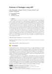
The following input graph is adapted from Goodrich & Tamassia’s data structures textbook. It shows several available
flights between U.S. airports, with their distances in miles. We would like to get from a friend’s house, 10 miles from
Boston (BOS), to our destination, 20 miles from Chicago (ORD).
2582
187
FriendHouse
10
BOS
SFO
802
1391
JFK
1090
1258
1121
MIA
802
DFW
1235
2342
ORD
20
MyHouse
1749
LAX
Shortest Paths
If we work things out
“FriendHouse” is
Destination
FriendHouse
BOS
JFK
MIA
DFW
ORD
MyHouse
SFO
LAX
by hand (or just ask Dyna) we will discover that the shortest path to each node from
Total
0
10
197
1268
1588
2390
2410
2779
2823
This is encoded into Dyna, using strings to identify vertices of the graph, thus:
edge("BOS","JFK")
edge("BOS","MIA")
edge("JFK","DFW")
edge("JFK","SFO")
edge("JFK","MIA")
edge("MIA","DFW")
edge("MIA","LAX")
edge("DFW","ORD")
edge("DFW","LAX")
edge("ORD","DFW")
edge("LAX","ORD")
:=
:=
:=
:=
:=
:=
:=
:=
:=
:=
:=
187.
1258.
1391.
2582.
1090.
1121.
2342.
802.
1235.
802.
1749.
1.2. Shortest Path in a Graph
5
Dyna Documentation, Release 0.4 git=31acba2
edge("FriendHouse","BOS") := 10.
edge("ORD","MyHouse") := 20.
edge pairs that are not specified are said to be null; that is, they have no value, and can be thought of as the identity
of the aggregator min=, or +∞, meaning “You can’t get there directly from here.”
And of course, we need to specify whence we come and where it is we would like to end up:
start := "FriendHouse".
end
:= "MyHouse".
1.2.2 Run the program
We can run this program in the interpreter:
./dyna -i examples/dijkstra.dyna
We are met with the conclusions, which include all the data we fed in as well as a pile of path assertions. Of course,
that’s not so useful, necessarily, so let’s just ask for the answer:
:- query goal
out(0) := [(2410, {})]
As we can see, the total weight of the shortest path is 2410. What happens, though, if we realize that we will be by
the airport anyway?
:- start := "BOS".
=============
goal := 2400
out(0) := [(2400, {})]
path(’BOS’) := 0
path(’DFW’) := 1578
path(’FriendHouse’) := None
path(’JFK’) := 187
path(’LAX’) := 2813
path(’MIA’) := 1258
path(’MyHouse’) := 2400
path(’ORD’) := 2380
path(’SFO’) := 2769
start := ’BOS’
And just like that, the total path weight from start to end is now 2400. The system also tells us a number of
potentially interesting things:
• The system has in fact computed the revised path costs to each other vertex.
• There is no path from "BOS" to "FriendHouse" (thus None).
• A query we had made earlier has changed its answer.
1.2.3 Explaining Answers
bug
We do not yet have a good mechanism implemented, though it’s just a matter of time. See issue 1.
6
Chapter 1. Tutorial
Dyna Documentation, Release 0.4 git=31acba2
1.2.4 Understanding The Program
Simply stated, this program looks for all paths from the vertex indicated by start. Formally, the technique currently
used is called agenda-driven semi-naive forward chaining 1 .
Inference Rules
The first inference rule states that there is no distance on the degenerate path that does not go anywhere.:
path(start) min= 0.
Alternatively, there is a path to vertex B if there is a path to some vertex A such that an edge connects A to B.:
path(B) min= path(A) + edge(A,B).
The final rule merely says that we are looking for the best path to the vertex indicated by end.:
goal min= path(end).
Inference Rules As Equations
But what are the min= and + doing? In fact, the inference rules are equations. They state how to find the values of all
pathto and goal items.
Those items have values just like the hello, world and goal items in the previous example. But this program is
more complicated. It involves lots of different pathto items for different airports, distinguished from one another by
their arguments: pathto("JFK"), pathto("MyHouse"), etc. These items may all have different values.
Why These Particular Equations?
Assuming that each edge‘s value represents its length in the input graph, the rules are carefully written so that
pathto(V)‘s value will be the total length of the shortest path from the start vertex to vertex V.
In principle, there are several ways to get to V: one can get there by an edge from start or an edge from some other
U. The min= operator finds the minimum over all these possibilities. Think of it as keeping a running minimum (just
as += would keep a running total). In particular, pathto(V) is found as min(edge(start, 𝑉 ), min𝑈 pathto(𝑈 ) +
edge(𝑈, 𝑉 )) which involves minimizing over all possible U.
If there are no paths to V, then pathto(V) is a minimum over no lengths at all. Dyna specifies that items receiving
no inputs take on the special value null, which is the identity of every aggregator and a zero of every expression. Since
we aggregate answers with min=, null approximates +∞.
1.2.5 Deriving The Graph From Rules
There’s nothing that mandates that edge weights be the base case; we could also derive edge facts from other facts,
such as position and reachability. An example is available in examples/dijkstra-euclid.dyna (or here).
1 There are a multitude of inference algorithms for logic programming. We would like to think that [filardo-eisner-2012] provides a good
overview as well as explaining the basics of what will become Dyna 2’s inference algorithm.
1.2. Shortest Path in a Graph
7
Dyna Documentation, Release 0.4 git=31acba2
1.2.6 Endnotes
1.3 When Things Go Wrong
1.3.1 Impossible Requests
What happens if a Dyna program attempts to divide by zero, as in:
a += 1 / b.
b += 0.
If this is the entirety of the program and no changes are forthcoming (e.g., we are not in interactive mode) then the
semantics of this program include division by zero, and so must be an error. What happens when we attempt to run it?
Our interpreter produces a chart with an annotation:
Charts
============
a/0
=================
b/0
=================
b
:= 0
Errors
============
because b is 0:
division by zero
in rule test.dyna:4:1-test.dyna:4:12
a += 1 / b.
This last Errors display indicates that the answers available in the Charts section is not reliable.
Caution: Any error is potentially global! While it might be possible for some programs to more accurately track
errors, currently our implementation does not. The net effect of this is that if ever the interpreter produces an
Errors section, then the entire chart must be considered suspect.
If we run the interactive interpreter and add the rule b += 1., the error condition has cleared as it should. If we then
add b += -1., it will return.
1.3.2 Non-Termination
Productive Nontermination
As mentioned before, Dyna2 currently uses agenda-driven semi-naive forward chaining for its reasoning. This algorithm has several excellent theoretical properties, but suffers from a potentially show-stopping problem: it might not
stop.
A Dyna program which includes a definition of the Fibonacci numbers (e.g., examples/fib.dyna)
fib(1) += 1.
fib(2) += 1.
fib(X) += fib(X-1) + fib(X-2).
8
Chapter 1. Tutorial
Dyna Documentation, Release 0.4 git=31acba2
will compile and be accepted by the interpreter, but will attempt to prove a fib item for every positive natural number!
Clearly, this task is going to take a while.
If your program does go away for longer than you expect, it is entirely possible that it is caught in such an infinite
loop. In that case, you may send it a SIGINT by hitting Control-C. The interpreter will then print out the chart as far
as it had determined it. If this is far bigger than expected, your program probably has a productive infinite loop.
Fixing The Fib Example
One way out of this problem is to impose a limit on the program, by writing instead something like:
f(X) += f(X-1) + f(X-2) for X < lim.
lim := 10.
This will limit the system to proving the first lim Fibonacci numbers. Of course, that can expand or contract as you
define lim.
Counting To Infinity
Unfortunately, another kind of nontermination error can arise in cyclic programs, which is not so easy to fix: the
so-called count-to-infinity problem.
If we were to have examples/dijkstra.dyna loaded in the interpreter and then run
:- start := "NoSuch".
Where there is no such "NoSuch vertex, the interpreter will appear to be pondering this change to the universe for “a
while”, as we say. If we interrupt it (with Control-C) after a while, the chart will contain, among other things:
path/1
=================
path("DFW")
path("LAX")
path("MyHouse")
path("NoSuch")
path("ORD")
path("SFO")
:=
:=
:=
:=
:=
:=
10124432
10124063
10122046
0
10123630
2779
This arises from the fact that our graph contains a cycle:
edge("DFW","ORD") := 802.
edge("ORD","DFW") := 802.
edge("LAX","ORD") := 1749.
Note that it is also possible to “count to infinity” in other directions, such as by counting down to −∞ or by approaching a finite solution but as in Zeno’s paradox.
bug
There is, as of yet, no good solution to this problem; the best work-around might just be to start the program over.
1.4 What is Dyna?
[sec:intro]
Dyna
1.4. What is Dyna?
9
Dyna Documentation, Release 0.4 git=31acba2
is a simple and straightforward programming language that you’ll be using in the assignments for this course. It’s
being developed at Johns Hopkins by Prof. Jason Eisner, Nathaniel Wesley Filardo, and Tim Vieira, among other
contributors.
If you have any experience programming, then Dyna will probably look very different from other languages you’ve
seen. That’s because Dyna is very high-level, and because it’s a declarative language. The rest of this section explains
what those terms mean, for those who are curious. You’re also welcome to skip directly to Section [sec:basics], which
explains the basics of Dyna and shows you some simple examples. After that, Section [sec:count] shows you how to
use Dyna to compute unigram and bigram probabilities from a corpus.
1.4.1 High-Level Languages
A high-level language is a programming language where the computer does much of the work for you. High-level
languages abstract away from the messy details; the higher-level a programming language is, the more levels of
abstraction it will contain.
When computer science first began, only very low-level languages existed. In the lowest-level languages, called
assembly languages, programmers had to provide a detailed set of instructions for the computer to follow. In order to
add two numbers, for instance, the programmer might have to write something that looked like “load the first number
from memory location X; load the second number from memory location Y; add them together; store the result in
memory location Z”.
As you might imagine, these kinds of programs were quite cumbersome to write, and so programmers developed
higher-level languages that could abstract away some of these details. In these languages, a compiler or interpreter
is used to translate from high-level instructions down into low-level assembly language commands. The compiler
or interpreter’s challenge is to find the most efficient low-level instructions that it can. This is harder for higherlevel languages, since the compiler has to do more translation to get the programs down to assembly code. But over
time, as compilers have gotten smarter and computers have gotten faster, programmers have been able to switch to
progressively higher-level languages without needing to worry about efficiency. More and more messy details of the
programming process have been abstracted away.
To give you some examples, C is an old compiled language that is still widely used. It’s higher-level than assembly,
because you can write “Z = X + Y” instead of the sequence of load/add/store instructions shown above, but you still
have to deal with some memory management. Languages like Java and Python are higher-level than C. In both Java
and Python, you don’t need to worry about managing the memory explicitly, and a lot of common programming tools
(for instance data structures like lists, hash tables, and sets) are built in. The highest-level language of all would be
a natural language; you would simply tell the computer, in English, what you wanted the program to do, and the
compiler would go off, with no further effort on your part, and figure out how to do what you asked.
“Programming” using plain English will have to wait until we’ve solved NLP, but in the meantime, a language like
Dyna is about as close as you’re going to get. In Dyna, if you want to know the value of something, you don’t need to
give explicit instructions on how to compute it. You just describe what the value looks like, and the Dyna interpreter
will figure out on its own how to find it efficiently. We realize this is a bit vague; you’ll see examples later in the
tutorial. In particular, if you’ve encountered Dijkstra’s algorithm for finding the shortest path in a graph, you may be
surprised to learn that the Dyna version can be written in just three lines.
1.4.2 Declarative Languages
Dyna is a declarative language. Declarative programming is one of many programming paradigms. Like high-level
vs. low-level, programming paradigms are another way in which languages can differ from one another. When you
write a program, you are asking the computer to calculate a specific answer for you. Different programming paradigms
express this request in different ways.
If you have any programming experience, then you’ve probably encountered the imperative paradigm. In this
paradigm, a program is a list of instructions that the computer needs to execute: “while condition is true, do some-
10
Chapter 1. Tutorial
Dyna Documentation, Release 0.4 git=31acba2
thing”. There’s also the object-oriented paradigm, used by languages like Java, where computation involves the creation and manipulation of objects. Languages like Lisp and Haskell follow the functional paradigm, where everything
is expressed in terms of functions.
And Dyna follows the declarative paradigm, where instead of giving the computer instructions, you just describe what
the solution looks like. Instead of telling the computer how to do something, you just tell it what you want it to
compute, and it figures out the “how” part for you. For example, in most languages, if you want to sort a list of values,
you’ll need to write out a sorting algorithm like bubblesort or mergesort. In a declarative language, you might specify
list sorting as follows:
given a list L, find a new list M such that: - M is a permutation of L - M’s elements appear in sorted order
The compiler would need to figure out a sorting algorithm on its own. As you might imagine, declarative languages
are necessarily very high-level, and writing efficient compilers/interpreters for them is quite challenging.
Jason teaches a whole course on declarative languages, so if you’re curious, make sure to check out the website:
<http://cs.jhu.edu/~jason/325/>.
1.5 The Basics of Dyna
[sec:basics]
This section will explain the basics of Dyna. You’re encouraged to follow along with the tutorial by trying everything
out yourself.
To use Dyna, first log into your account on the CLSP server. When you’re on the machine a14, type dyna at the
command line (it might take a few seconds to load). You will then see the Dyna prompt.
username@a14$ dyna
>
To exit Dyna, you can type exit at the Dyna prompt:
> exit
username@a14:~$
1.5.1 Defining Items in Dyna
Dyna is a lot like a (very powerful) spreadsheet. In a spreadsheet, you have cells, and you can give them values in two
ways: by assigning them values directly, or by defining them in terms of other chart cells. For instance, you might
define the cell C1‘ to be the sum of cells A1 and B1, whose values you have typed in by hand.
Let’s try this in Dyna. The Dyna equivalent of a chart cell is called an item. So let’s create three items in Dyna, called
a, b, and c. First we’ll define a and b:
> a := 5.
Changes
=======
a = 5.
> b := 7.
Changes
=======
b = 7.
1.5. The Basics of Dyna
11
Dyna Documentation, Release 0.4 git=31acba2
Note:
to follow along with this tutorial, whenever you see a line that starts with the prompt >, you can type in the part of the
line which follows the prompt (and then press enter). Every line that does not begin with > is a reply from the Dyna
intepreter. So, in this example, you can enter the line a := 5., and Dyna will respond to it and then give you another
prompt, at which point you can type b := 7.
The lines of Dyna code that we typed (a := 5. and b := 7.) are called rules. Each time you type a rule into
Dyna, the interpreter tells you which values have been updated as a result. In the case of a := 5. the value of a has
been updated to 5. (Previously, a didn’t even exist, and so it had no value.)
Now let’s define c as the sum of a and b:
> c += a + b.
Changes
=======
c = 12.
This rule is similar to the previous two, but as you can see, the first two rules defined a and b using numeric values,
while this rule defines c in terms of other Dyna items.
You’ll also notice that the first two rules use :=, while the last rule uses +=. These are called aggregators. Each
Dyna rule helps to define the value of an item. The item appears to the aggregator’s left, and a contribution to its value
appears to the aggregator’s right.
A single item may appear on the left of many rules, so it may get many contributions. The aggregator specifies
how to aggregate (combine) those contributions into a single value for the item. The aggregator += says to add up the
contributions, so each += rule says “augment this item’s definition by adding in this new contribution”. The aggregator
:= says to use the last contribution only, so each := rule says “redefine this item to equal this new contribution”.
When there is only one contribution to an item, it usually doesn’t matter how the contributions are aggregated. So the
rules above just define a, b, and c to each equal a single contribution. But we’ll see examples later on where += and
:= do have different effects; we’ll also see different aggregators.
Watch Out for Errors
Make sure to end your rules with a period, or you’ll get an error:
> a := 5
ERROR: Line doesn’t end with period.
It’s also important to get the syntax of the rule correct. A rule in Dyna should contain these five things in this order:
• an item (such as a)
• an aggregator (such as +=)
• a value (such as 5), or an expression which has a value (such as a + b)
• an optional condition (we haven’t seen these yet)
• a period to end the line
This means that you can’t, for instance, type 5 := a. If you do this, it will confuse Dyna greatly:
> 5 := a.
DynaCompilerError: Terribly sorry, but you’ve hit an unsupported feature
This is almost assuredly not your fault! Please contact a TA.
The rule at <repl> is beyond my abilities.
new rule(s) were not added to program.
12
Chapter 1. Tutorial
Dyna Documentation, Release 0.4 git=31acba2
(Actually, this would be your fault, but Dyna errs on the side of friendliness. And if you are having trouble writing a
program in Dyna, you are always welcome to contact a TA.)
Dyna is Dynamic
Now let’s return to our example. We’ve defined three items, a, b, and c. The item c is defined in terms of a and b.
Like a spreadsheet, Dyna is dynamic, so if you change the value of a or b, c changes accordingly:
> a := 1.
Changes
=======
a = 1.
c = 8.
Again, after you type a rule into Dyna, it prints out all the items whose values have been updated. This time two items’
values were updated, a and c.
Defining an Item over Multiple Lines
Earlier, we defined c in one line, like this:
c += a + b.
But we also could have defined it in two lines, like this:
c += a.
c += b.
The += aggregator is designed to be used in multi-line definitions like this. Recall that each time you use +=, it updates
the item’s value by adding the new value into it.
It may seem strange to define c over two lines instead of one. In Section [subsec:itemswithvars], you’ll see an example
of why this ability is useful. It turns out that it makes the += aggregator (and all the other aggregators) very powerful.
In fact, this is why they’re called aggregators: they aggregate a collection of rules into a single definition for an item.
Retracting a Rule
Suppose we want to try changing the definition of c‘ from
c += a + b.
to
c += a.
c += b.
as shown in the previous section. We can’t just type in the rules from the second box, because c already has the value
a + b, and adding more rules will just add to this value:
> c += a.
Changes
=======
c = 9.
> c += b.
1.5. The Basics of Dyna
13
Dyna Documentation, Release 0.4 git=31acba2
Changes
=======
c = 16.
So what do we do if we want to switch c’s definition to the new version? We have to retract the rule c += a + b.
We can do this using the retract_rule command in Dyna:
> retract_rule X
Here, X is the index of the rule you want to retract. You can find out a rule’s index by typing the command rules,
which lists all the rules that have been defined so far.
> rules
Rules
=====
0: a :=
1: b :=
2: c +=
3: a :=
4: c +=
5: c +=
5.
7.
a + b.
1.
a.
b.
From this, we know that we want to retract rule 2:
> retract_rule 2
Changes
=======
c = 8.
If we type the command rules again, we can see that our previous definition of c has disappeared:
> rules
Rules
=====
0: a :=
1: b :=
3: a :=
4: c +=
5: c +=
5.
7.
1.
a.
b.
A last note on retracting rules: make sure you don’t end the rule-retraction command with a period, or Dyna will get
confused:
> retract_rule 2.
Please specify an integer. Type ‘help retract_rule‘ to read more.
Rearranging Rules
In many cases, rule order in Dyna doesn’t matter. So right now, we’ve defined these rules in this order:
a
b
a
c
c
:=
:=
:=
+=
+=
14
5.
7.
1.
a.
b.
Chapter 1. Tutorial
Dyna Documentation, Release 0.4 git=31acba2
But we could have also defined them in this order:
c
b
a
c
a
+=
:=
:=
+=
:=
a.
7.
5.
b.
1.
Here, we’ve made a number of changes. For one thing, we’ve switched the order of the rules a := 5. and b :=
7.. Unsurprisingly, this doesn’t affect their values.
What might be more surprising is that we can move the rule c += a. to the beginning, before a is even defined.
(We could have also moved the rule c += b. to the beginning if we had wanted to.)
How does this work? Well, when we first type c += a., a‘s value is undefined. This means that c is the sum of
something undefined, making c‘s value undefined as well. But not for long! As soon as we add the rule a := 5.,
then c‘s value, which depends on the value of a, gets updated. (The addition of the rules c += b. and a := 1.
also update the value of c, of course.)
To make this clear, let’s retract all the rules we added before, and now add them in the new order. This is what Dyna
prints out:
> c += a.
> b := 7.
Changes
=======
b = 7.
> a := 5.
Changes
=======
a = 5.
c = 5.
> c += b.
Changes
=======
c = 12.
> a := 1.
Changes
=======
a = 1.
c = 8.
As you can see, some of the intermediate values are different. In particular, Dyna prints nothing after we add c +=
a. That’s because nothing has changed, since c‘s value was undefined before we added the rule, and it’s undefined
after we’ve added the rule too.
The important thing to note is that the final result remains unchanged. These five rules, taken together as a set, define
the values of a, b, and c. For the most part, reordering the rules within the set won’t affect the values.
The big exception is the := aggregator. It defines an item’s value as the last rule that applies to that item. So, if we
had switched the order of the a rules like this:
a := 1.
a := 5.
1.5. The Basics of Dyna
15
Dyna Documentation, Release 0.4 git=31acba2
then a’s final value would be 5, and c‘s value would reflect this as well.
A final note on terminology: a, b, and c are all terms. When a term has a value, we call it an item. When a term’s
value is undefined, we say that the term has the value null.
1.5.2 Items with Variables
[subsec:itemswithvars]
As we said at the beginning, Dyna is a lot like a very powerful spreadsheet. But an Excel spreadsheet has a fixed 2D
structure of rows and columns. This means that every cell in a spreadsheet is defined in terms of a letter and a number,
e.g. A1 or H75.
A Dyna program, on the other hand, is not restricted in this way. So far, we’ve seen items named a, b, c, and you can
also have longer names like sum and veryLongName. But all of these names are just plain strings of text. Often,
you will want to define more complex names, to give your items more structure:
> d(1) := 5.
Changes
=======
d(1) = 5.
> d(2) := 10.
Changes
=======
d(2) = 10.
> d(3) := 19.
Changes
=======
d(3) = 19.
In this example, d is called a functor. The functor d takes one argument. Functors make it possible to refer to many
items at the same time:
> dtotal += d(I).
Changes
=======
dtotal = 34.
As you can see, this rule adds up d(1), d(2), and d(3). How does it do this? It turns out that the rule dtotal +=
d(I). doesn’t just describe a single addition to dtotal‘s value, but a whole set of additions, one for each item that
pattern-matches to d(I). I is a variable that will match any argument of the functor d. So, in this example, the line
dtotal += d(I). is equivalent to the following three rules:
dtotal += d(1).
dtotal += d(2).
dtotal += d(3).
But this takes a lot longer to write, and is much less general. With the original definition, if we added a new item d(4),
it would automatically update dtotal‘:
> d(4) := 6.
Changes
16
Chapter 1. Tutorial
Dyna Documentation, Release 0.4 git=31acba2
=======
d(4) = 6.
dtotal = 40.
This wouldn’t work for the three-line definition. You’d have to add a new line like this:
dtotal += d(4).
The rule dtotal += d(I). is much like the mathematical equation $d_{text{total}} = sum_I d(I)$, while using
three separate rules is like writing $d_{text{total}} = d(1) + d(2) + d(3)$. If d(4) is defined, the first equation would
include it in the sum automatically, while the second equation qould ignore it.
In the next section, we’ll look at some more examples with variables. First, though, how can we tell a variable from a
functor? It’s easy: a variable always starts with a capital letter, and a functor always starts with a lowercase letter.
So, earlier, we wrote dtotal += d(I). If we now write dtotal2 += d(a), we will see that it gives a completely different answer:
> dtotal2 += d(a).
Changes
=======
dtotal2 = 5.
What happened here? Well, a is a functor, not a variable. Recall from earlier that a has the value 1. So, in this
example, a evaluates to 1, and thus d(a) becomes equal to d(1)‘, which equals ‘‘5.
Exercise:
What does d(2*a+1) evaluate to?
Some More Examples with Variables
Here’s another example containing a Dyna rule with a variable:
e(1)
e(2)
f(1)
f(2)
g +=
:= 1.
:= 2.
:= 4.
:= 5.
e(I)*f(I).
This turns out to be equivalent to:
g += e(1)*f(1).
g += e(2)*f(2).
That is, the variable I‘ appears twice in g += e(I)*f(I)., so both instances of I have to pattern-match to the
same thing. That’s because the rule is saying “for all I such that e(I) and f(I) are defined, add e(I)*f(I) to
the definition of g”. (Note: the * is a multiplication sign.)
If you use two different variables, the result will be different, because the variables can pattern-match independently:
h += e(I)*f(J).
This is equivalent to:
h
h
h
h
+=
+=
+=
+=
e(1)*f(1).
e(1)*f(2).
e(2)*f(1).
e(2)*f(2).
1.5. The Basics of Dyna
17
Dyna Documentation, Release 0.4 git=31acba2
In other words, the rule h += e(I)*f(J). says “for all I, J pairs such that e(I) and f(J) are both defined, add
e(I)*f(J) to the definition of h”.
Functors with Multiple Arguments
So far, we’ve seen functors with one argument, such as d(1). We’ve also seen functors with zero arguments — it
turns out that the items a, b, and c that we defined at the beginning are actually just functors with no arguments. a is
equivalent to a(), but Dyna allows you to leave out the parentheses for zero-argument functors, to make them easier
to type.
Of course, in Dyna, you aren’t limited to zero- or one-argument functors. You can define functors with as many
arguments as you like. For instance, if you were making the Dyna equivalent of a grading spreadsheet, you might have
a functor with two arguments that lists each student’s grade on each exam:
grade("Steve", "midterm") := 85.
grade("Steve", "final") := 90.
grade("Jamie", "midterm") := 94.
grade("Jamie", "final") := 97.
grade("Anna", "midterm") := 82.
grade("Anna", "final") := 89.
Now suppose we want to compute each student’s total score. Also, to make things more interesting, suppose that the
two exams are weighted differently. So let’s add a new functor specifying the percent each exam contributes to the
student’s final grade in the class.
weight("midterm") := 0.35.
weight("final") := 0.65.
Then we can compute the final grade for each student like this:
finalgrade(I) += grade(I,J)*weight(J).
The names of the variables don’t matter; we’ve just chosen I and J because they’re conventional variable names. But
often, you’ll want to choose more meaningful variable names to make your rules more readable. The following rule is
equivalent to the previous one:
finalgrade(Student) += grade(Student,Exam)*weight(Exam).
We can also have rules which contain both variables and atoms. (An atom is an argument to a functor. Types of
atoms include strings in quotes, like "Steve", and numbers, like 903 or 3.14159. Variables don’t count as atoms,
because they stand in place of atoms.) For an example of a rule which contains both variables and atoms, suppose we
only wanted to compute Steve’s grade, and we didn’t care about Jamie or Anna. Then we could use the following rule:
finalgrade("Steve") += grade("Steve",Exam)*weight(Exam).
So now we’ve seen functors with zero, one, and two arguments. But remember, functors can have as many arguments
as you like:
> x(1,2,3,4,5,6,7,8,9,"panda") := 2.
Changes
=======
x(1,2,3,4,5,6,7,8,9,"panda") := 2
Also, it’s important to note that the same functor can appear with different numbers of arguments. So, instead of
finalgrade(Student) += grade(Student,Exam)*weight(Exam).
we could have written
18
Chapter 1. Tutorial
Dyna Documentation, Release 0.4 git=31acba2
grade(Student) += grade(Student,Exam)*weight(Exam).
Now we have two versions of the functor grade, one with one argument and another with two arguments. This is
similar to how the English verb “eat” has both intransive and transitive versions.
Note that these two versions of grade don’t interfere with each other during pattern matching, since any use of
grade must either pattern match to the one-argument version or the two-argument version, but it can’t pattern match
to both at the same time. So suppose we say:
allgrades += grade(Student).
This rule can only match the one-argument version of grade.
1.5.3 Writing a Program in Dyna
We’ve seen a lot of basic examples in this section, and we’re almost ready to move on to real NLP applications. First,
though, you’ll need to know how to write an actual program in Dyna. So far, we’ve just been typing rules directly into
the Dyna interpreter. This is very useful for playing around with Dyna, but it’s quite inconvenient if you want to run
the same program more than once. You would have to retype the rules into the interpreter every time you wanted to
run it.
Fortunately, you can save your rules in a file, and Dyna will read them. For instance, open up your favorite command
line text editor (e.g. nano, vim, emacs), and type the rules from our grading example:
grade("Steve", "midterm") := 85. grade("Steve", "final") := 90.
grade("Jamie", "midterm") := 94. grade("Jamie", "final") := 97.
grade("Anna", "midterm") := 82. grade("Anna", "final") := 89.
weight("midterm") := 0.35. weight("final") := 0.65.
finalgrade(Student) += grade(Student,Exam)*weight(Exam).
Save this file as anything. Mine is called grades.dyna, but you can name it carrot if you like. Now run Dyna
on your program like this:
username@a14:$ dyna grades.dyna
Once Dyna has loaded the program, it will print out a list of all the items that are currently defined. The items are
organized by functor, and the functors are listed in alphabetical order. Here’s what the output looks like for our
program:
Solution
========
finalgrade/1
============
finalgrade("Anna") = 86.55.
finalgrade("Jamie") = 95.95.
finalgrade("Steve") = 88.25.
grade/2
=======
grade("Anna","final")
grade("Anna","midterm")
grade("Jamie","final")
grade("Jamie","midterm")
grade("Steve","final")
grade("Steve","midterm")
1.5. The Basics of Dyna
=
=
=
=
=
=
89.
82.
97.
94.
90.
85.
19
Dyna Documentation, Release 0.4 git=31acba2
weight/1
========
weight("final")
= 0.65.
weight("midterm") = 0.35.
You’ll notice that the program exited after it was done printing this. You can also run the Dyna interpreter interactively
after loading a program:
username@a14:~$ dyna -i grades.dyna
Once the program is loaded, you can add rules as you did earlier. Now, however, the rules you add may interact with
the rules in the original program. For instance, let’s add a new student:
> grade("Keith","midterm") := 76.
Changes
=======
finalgrade("Keith") = 26.599999999999998.
grade("Keith","midterm") = 76.
> grade("Keith","final") := 87.
Changes
=======
finalgrade("Keith") = 83.15.
grade("Keith","final") = 87.
As you can see, when we add grade("Keith","midterm"), it creates an item finalgrade("Keith"),
using the rules finalgrade(Student) += grade(Student,Exam)*weight(Exam).
and
weight("midterm") := 0.35. in the program we loaded.
Now observe what happens when we add the following rule:
> grade("Vanessa", "makeup midterm") := 100.
Changes
=======
grade("Vanessa","makeup midterm") = 100.
As you can see, it does not create an item finalgrade("Vanessa"). Why is this? Consider what happens
when the rule finalgrade(Student) += grade(Student,Exam)*weight(Exam). tries its patternmatching on grade("Vanessa", "makeup midterm"). The variable Student binds to "Vanessa" and
the variable Exam binds to "makeup midterm". But there’s no item weight("makeup midterm") in our
program, so the overall pattern-matching fails.
What is a Dyna Program?
We are finally in a position to state what a Dyna program actually is. A Dyna program is simply a list of rules which
define a set of items. (As we saw earlier, an item may be defined using multiple rules.)
When you use the Dyna interpreter, you are slowly specifying a Dyna program, one rule at a time. If you’re using the
Dyna interpreter with a program that you loaded from file, then each rule you type into the interpreter extends that
program.
Note that when you close the Dyna interpreter, it doesn’t save any of the rules that you typed. They exist for that
session only and don’t affect the original program. So if you look at the file grades.dyna‘, you will see that it contains
no mention of Keith or Vanessa.
20
Chapter 1. Tutorial
Dyna Documentation, Release 0.4 git=31acba2
1.5.4 The Help Command
One final note before we continue on to the next section. We have covered some commands already in this tutorial, and
we will cover more in the next section, but we won’t have time to explain every feature of Dyna. Fortunately, Dyna
contains documentation which will help you if you don’t understand how to use a command. To see which commands
are documented, you can type help at the Dyna prompt like this:
> help
Documented commands (type help <topic>):
========================================
EOF exit load post query retract_rule rules run sol trace vquery
Undocumented commands:
======================
help
To get help for a specific command, you can type help followed by that command’s name:
> help exit
Exit REPL by typing exit or control-d. See also EOF.
1.6 Counting Words in a Corpus
[sec:count]
In this section, we’ll use Dyna to calculate unigram and bigram probabilities for a very small subset of the Brown
corpus.
1.6.1 The Brown Corpus
First, let’s take a look at the corpus. We’ve stored it in a file called brown.txt, which you can get by typing the
following command:
wget http://cs.jhu.edu/ jason/licl/brown.txt
(The wget command retrieves a file from the internet, specified by its URL.)
In order to look at the file’s contents, you can use this command:
username@a14: $ less brown.txt
(The program less allows you to scroll up and down through a long piece of text to see what’s in it. You can type q
to quit less and return to the command line.)
As you can see, the file contains lines like this:
You should hear the reverence in Fran’s voice when she said “ Baccarat ” or “
Steuben ” or “ Madame Alexander ” .
This looks like an ordinary sentence, except that something strange has happened to the punctuation. That’s because
this sentence has been tokenized, which means that it’s been split into meaningful units that the computer can process
more easily. If we’re counting up the occurrences of the word “house” in the corpus, for instance, we don’t want
to have to consider “house” and “house,” and “house.”. (Note that tokenization is not as simple as just detaching
punctuation from words. For instance, we can’t just make a rule that separates all periods, because we want them to
stay attached in titles like “Dr.”.)
1.6. Counting Words in a Corpus
21
Dyna Documentation, Release 0.4 git=31acba2
Different tasks will call for different kinds of tokenization. Some corpora will separate out the possessive clitic, so
“Fran’s” in the above sentence would be “Fran ’s”. One could also tokenize the corpus by morpheme instead of word.
People who are creating or using corpora might use other preprocessing techniques as well. Many corpora remove
the capitalization from the beginning of the sentence; the Brown corpus hasn’t done this.
1.6.2 Loading the Brown Corpus into Dyna
Now we need to load the corpus into Dyna. Fortunately, Dyna has a feature called loaders which makes this very easy.
In order to load our small subset of the Brown corpus, you can type the following into the Dyna interpreter:
> load brown = matrix("brown.txt", astype=str)
If you type sol at the Dyna prompt like this:
> sol
then Dyna will print out a full list of all the items and their values. If you do this, you can see that the data we loaded
is very long, and that the bottom looks like this:
...
brown(1052,0) = "From".
brown(1052,1) = "what".
brown(1052,2) = "I".
brown(1052,3) = "was".
brown(1052,4) = "able".
brown(1052,5) = "to".
brown(1052,6) = "gauge".
brown(1052,7) = "in".
brown(1052,8) = "a".
brown(1052,9) = "swift".
brown(1052,10) = ",".
brown(1052,11) = "greedy".
brown(1052,12) = "glance".
brown(1052,13) = ",".
brown(1052,14) = "the".
brown(1052,15) = "figure".
brown(1052,16) = "inside".
brown(1052,17) = "the".
brown(1052,18) = "coral-colored".
brown(1052,19) = "boucle".
brown(1052,20) = "dress".
brown(1052,21) = "was".
brown(1052,22) = "stupefying".
brown(1052,23) = ".".
Each item in the data takes the form brown(Sentence,Position), and its value is the word at that position of
that sentence. (The indices start at 0, so the first word in this sentence is brown(1052,0), not brown(1052,1).
Similarly, words in the first sentence take the form brown(0,Position).)
Now let’s look at the load‘ command in more detail. Recall that it looks like this:
> load brown = matrix("brown.txt", astype=str)
The word load at the beginning tells Dyna that we want to use a loader. brown is the name of the functor to load the
data into. If we had typed load red = ... instead, we would have gotten items that looked like red(1052,0)
and so on. matrix is the name of the specific loader we are using; it loads each word as a separate item. As you
might imagine, "brown.txt" tells Dyna which file to load. Lastly, astype=str tells Dyna to treat the words in
the file as strings, and not, for instance, as numbers.
22
Chapter 1. Tutorial
Dyna Documentation, Release 0.4 git=31acba2
You may also find the tsv loader useful at some point. Instead of loading each word as an item, it loads each line
as an item. For instance, suppose you had a text file which contained the rules of a context free grammar, along with
their probabilities:
1 S NP VP
0.5 ROOT S .
0.25 ROOT S !
0.25 ROOT VP !
0.5 VP V
0.5 VP V NP
...
In this (imaginary) file, the first column is the probability, the second column is the left-hand side of the rule, and the
remaining columns form the right-hand-side of the rule. You could load in this data using tsv like this:
> load grammar_rule = tsv("grammar.txt")
> sol
grammar_rule/4
==============
grammar_rule(4,"0.5","VP","V") = true.
grammar_rule/5
==============
grammar_rule(0,"1","S","NP","VP") = true.
grammar_rule(1,"0.5","ROOT","S",".") = true.
grammar_rule(2,"0.25","ROOT","S","!") = true.
grammar_rule(3,"0.25","ROOT","VP","!") = true.
grammar_rule(5,"0.5","VP","V","NP") = true.
...
There are a few things to note. First of all, the words in the file must be separated by tabs in order for tsv to work.
(This is why the loader is called tsv — it’s a standard abbreviation for “tab-separated values”.) Secondly, since the
rules of this grammar have different numbers of nonterminals, we get two versions of the grammar_rule functor,
one with four arguments and another with five. Lastly, the first argument to the functor is always the row number in
the file.
We will not actually be using tsv in this tutorial, but you may find it helpful for your homework.
1.6.3 Counting Words
Now that we’ve loaded the corpus using the matrix loader, we can use Dyna to collect the unigram counts (that is,
we’ll determine how many times each word appears in the corpus):
count(W) += 1 for W is brown(Sentence,Position).
(We’ll explain how this rule works in Section [subsec:conditions], so don’t worry if it doesn’t make any sense.)
When you enter this rule, Dyna prints out a long list containing the count for each word type that appears in the corpus.
The bottom of the list should look like this:
...
count("written") = 1.
count("wrong") = 2.
count("wrote") = 7.
count("wry") = 1.
count("yapping") = 1.
count("yaws") = 1.
count("year") = 8.
1.6. Counting Words in a Corpus
23
Dyna Documentation, Release 0.4 git=31acba2
count("yearly") = 1.
count("yearning") = 1.
count("years") = 21.
count("yelled") = 1.
count("yellow") = 1.
count("yelping") = 1.
count("yes") = 1.
count("yet") = 3.
count("yore") = 1.
count("you") = 131.
count("you’ll") = 1.
count("you’re") = 9.
count("you’ve") = 4.
count("young") = 4.
count("youngest") = 1.
count("your") = 38.
count("yours") = 2.
count("yourself") = 1.
count("yourselves") = 4.
count("youth") = 2.
count("zounds") = 2.
These counts might seem a bit strange. The word “yore” appears just as often as “yourself” does, for instance. That’s
because we used a very small subset of the Brown corpus (just 1053 sentences). The smaller the corpus, the less
reliable the counts will be. With only 1053 sentences, it’s no wonder that we find some anomalies! But in a corpus of
a million sentences, it’s very unlikely that we’d still see “yore” as frequently as “yourself”.
By the way, in Computational Linguistics terminology, the brown(Sentence,Position) items represent word
tokens while the count(W) items range over word type. A token is a specific instance of a generic word type. For
instance, brown(1052,14) and brown(1052,17) both have the value “the”. These two items represent two
different tokens, but only one word type.
1.6.4 Querying Dyna
As you’ve presumably noticed, the list of counts that Dyna printed is very long. What if you wanted to know the count
of the word and? Would you have to scroll all the way up to the top of the list?
It turns out that Dyna has a more convenient way of checking an item’s value, called a query:
> query count("and")
count("and") = 512
Queries are very simple. You just type the word query followed by the item whose value you want to know, and
Dyna will print that value.
If you query an item that doesn’t exist or has no contributions, Dyna will inform you that there are no results:
> query pajamas
No results.
You can also make more complicated queries, where you ask Dyna for the value of a whole expression, instead of just
a single item:
> query count("year") + count("years")
count("year") + count("years") = 29
24
Chapter 1. Tutorial
Dyna Documentation, Release 0.4 git=31acba2
Note that while rules end with a period, queries do not:
> query count("year") + count("years").
Queries don’t end with a dot.
Like rules, queries can contain variables. The following query would show us the count of every word:
> query count(W)
We can also mix atoms and variables in queries, just as we did with rules:
> query brown(57,Position)
brown(57,0) = "With".
brown(57,1) = "greater".
brown(57,10) = "this".
brown(57,11) = "time".
brown(57,12) = "a".
brown(57,13) = "little".
brown(57,14) = "more".
brown(57,15) = "to".
brown(57,16) = "the".
brown(57,17) = "left".
brown(57,18) = ".".
brown(57,2) = "precision".
brown(57,3) = "he".
brown(57,4) = "again".
brown(57,5) = "paced".
brown(57,6) = "off".
brown(57,7) = "a".
brown(57,8) = "location".
brown(57,9) = ",".
As you can see, this shows us the entirety of sentence 57, albeit not in the correct order. We can also view the first
word of each sentence using the following query:
> query brown(Sentence,0)
1.6.5 Rules with Conditions
[subsec:conditions]
Let’s return to our word-counting rule, and look at the details of how it works. Recall that the rule looks like this:
count(W) += 1 for W is brown(Sentence,Position).
This is our first example of a rule with a condition. The condition tells you when the rule should apply. In
this case, it applies once for each word token in the corpus, because each token will pattern-match to a different
brown(Sentence,Position) item. You can think of this rule as saying “For each Sentence‘ and Position
such that brown(Sentence,Position) is defined, let W‘ be the value of brown(Sentence,Position),
and add 1 to count(W).”
How does this rule work, exactly? A condition contains the word for followed by a boolean expression (that is, an
expression whose value is either true or false). The expression count("year") + count("years") is
not a boolean, since its value is the number 29‘. The expression count("year") > count("years"), on the
other hand, is a boolean whose value is false:
1.6. Counting Words in a Corpus
25
Dyna Documentation, Release 0.4 git=31acba2
> query count("year") > count("years")
count("year") > count("years") = false
Returning again to our word-counting rule, the expression W is brown(Sentence,Position) is true when W
is the value of brown(Sentence,Position). For instance, "what" is the value of brown(1052,1), so the
expression W is brown(1052,1) is true when W pattern-matches to "what".
For a slightly more complicated example, suppose you only wanted the counts of the words from the first 50 sentences
of the corpus. You would have to add an extra restriction to the condition:
count2(W) += 1 for (W is brown(Sentence,Position)) & (Sentence < 50).
Now, an item of the form brown(Sentence,Position) won’t pattern-match this rule unless Sentence <
50. (Note that we put parentheses around the two conditions to keep the Dyna parser from getting confused. If the
Dyna parser is getting confused, this is one thing you can try.)
Exercise:
How many different word types appear in the corpus?
1.6.6 Creating Probabilities from Unigram Counts
Now that we have the unigram counts, we can use them to determine the unigram probabilities for each word in the
corpus.
Recall that the unigram probability $p(w)$ of a word $w$ is $frac{c(w)}{c}$, where $c(w)$ is the count of word $w$,
and $c$ is the total number of word tokens in the corpus.
Exercise:
How can you use Dyna to count the total number of word tokens in the corpus? (Hint: the correct number turns out to
be 21695.)
After completing this exercise, you can use the total count of words in the corpus to compute the probability of each
word:
unigram_prob(W) := count(W) / totalcount.
1.6.7 Finding the Most Frequent Word
These counts and probabilities are nice because we can use them to discover interesting facts about the corpus. For
instance, we might ask, what is the most common word? What is that word’s frequency? What is that word’s probability?
We’ll first compute the mystery word’s frequency, using the following rule:
> highest_frequency max= count(W).
Changes
=======
highest_frequency = 1331.
As you can see, we’ve used a new aggregator, max=. The rule says that highest_frequency’s value should be
defined as maximum value of all the counts. That is, out of every item that pattern-matches to count(W), max=
picks the one with the highest value, and assigns that value to highest_frequency‘. Note that there is also a similar
aggregator called min= that finds the minimum.
26
Chapter 1. Tutorial
Dyna Documentation, Release 0.4 git=31acba2
The most common word in the corpus appears 1331 times. We can now use a query to check which word it is:
> query W for count(W) == highest_frequency
"," for count(",") == highest~f~requency = ","
As you can see, the most frequent word is... a comma. Well, that’s pretty boring. On the bright side, the query we
used to find it has an interesting structure. In particular, this example reveals that queries can contain conditions, and
those conditions work exactly the same way as they do in rules.
For another query with a condition, consider the following example, where we ask Dyna to show us all rules whose
counts are greater than 1000.
> query W for count(W) > 1000
"," for count(",") > 1000 = ","
Turns out it’s just the comma. If we lower the threshold to 900, we also get “the”:
> query W for count(W) > 900
"," for count(",") > 900 = ","
"the" for count("the") > 900 = "the"
Finally, to complete the example from this section, we can ask what the probability of the comma is:
> query unigram~p~rob(",")
unigram_prob(",") = 0.061350541599446876
It seems that approximately 6% of all the words in our corpus are commas.
Exercise:
Comma is the most common word overall. But what is the most common word to start a sentence with?
1.6.8 Computing Bigram Probabilities
Now let’s compute the bigram probabilities for this corpus. First, we’ll need to collect the bigram counts:
in_vocab(W) := true for count(W) > 0.
bigram_count(V,W) += 0 for in_vocab(V) & in_vocab(W).
bigram_count(V,W) += 1 for (V is brown(Sentence,Position)) & (W is brown(Sentence,Position+1)).
The third line should be the most straightforward. It increases the bigram count for the pair of words V‘, W whenever
W follows V in the corpus (i.e. they are in the same sentence and W’s position is V’s position plus 1).
The first and second line are a bit more complicated; they work together to make sure the count of each bigram starts
out at 0. This is important because, if a bigram never appears in the corpus, we want its count to be 0 instead of
undefined.
The first line determines which words appear in the corpus. It sets in_vocab(W) to the logical value true‘ for each
word W that appears in the corpus.
The second line adds 0 to the bigram count for each pair of words in the vocabulary. The second and third lines work
together to define bigram_count(V,W). Specifically, the second line adds 0 to the count of each bigram that could
appear in the corpus. The third line adds 1 whenever the bigram actually does appear.
(Unfortunately, at the time of writing this tutorial, Dyna is too slow to compute the results of the second rule in a
reasonable amount of time. When we tried this rule out, we got tired of waiting for Dyna, and so we typed Ctrl-C,
which tells Dyna to cancel whatever it’s currently doing.
1.6. Counting Words in a Corpus
27
Dyna Documentation, Release 0.4 git=31acba2
Why is Dyna so slow here? Well, there are 5017 word types in the corpus, meaning that there are approximately
$5017^2 = 25170289$ possible bigrams. Dyna naively tries to compute zeros for all of these. The right approach
would be to compute only the counts of bigrams that actually occur, and simply return zero by default for any other
bigram. A future version of Dyna will be able to figure that out.)
Now that we have the bigram counts, we can use them and the original counts to compute the bigram probabilities:
bigram_prob(V,W) := bigram~c~ount(V,W) / count(V).
As you can see, “the man” has a probability of around 0.002, while “man the” has a probablity of 0, because it never
appears in this corpus and we haven’t used any smoothing:
> query bigram_prob("the","man")
bigram_prob("the","man") = 0.002150537634408602
> query bigram~p~rob("man","the")
bigram~p~rob("man","the") = 0
Exercise:
What word is most likely after “the”, and how likely is it? What word is most likely after “of”? How about before “.”?
Exercise:
Define estimates of bigram probabilities that use add-$lambda$ smoothing. (Hint: define lambda := 1 and write
your defs in terms of lambda. You can change lambda and the estimated probabilities will change as well.) Can
you compute cross-entropy on a development corpus?
Exercise:
Using a similar approach to the one in this section, compute the trigram probabilities.
1.6.9 VQuery and Trace
We’ve now seen many examples of queries, both with and without conditions. In addition to the query command,
Dyna also has two other commands that you might find helpful: vquery and trace.
The regular query is designed for querying the value of an expression. On the other hand, vquery is designed for
investigating the variables that pattern-match to an expression.
To see the difference, suppose you want to know which bigrams have a count greater than zero, and what their counts
are. You could use a regular query like this:
> query bigram_count(V,W) for bigram_count(V,W) > 0
and it will spew something ugly like this:
...
bigram_count("yourself","to") for bigram_count("yourself","to") > 0 = 1
bigram_count("yourselves",",") for bigram_count("yourselves",",") > 0 =
bigram_count("yourselves","into") for bigram_count("yourselves","into")
bigram_count("yourselves","of") for bigram_count("yourselves","of") > 0
bigram_count("yourselves","on") for bigram_count("yourselves","on") > 0
bigram_count("youth","is") for bigram_count("youth","is") > 0 = 1
bigram_count("youth","worked") for bigram_count("youth","worked") > 0 =
bigram_count("zounds","’’") for bigram_count("zounds","’’") > 0 = 2
1
> 0 = 1
= 1
= 1
1
Or you could use vquery, which gives a much cleaner answer, in sorted order (though here, V and W are backwards):
28
Chapter 1. Tutorial
Dyna Documentation, Release 0.4 git=31acba2
> vquery bigram~c~ount(V,W) for bigram~c~ount(V,W) \> 0
...
57 where W="I", V=","
76 where W="the", V=","
76 where W="?", V="?"
88 where W="the", V="in"
106 where W=",", V="”"
111 where W=".", V="”"
115 where W="the", V="of"
130 where W="and", V=","
Another useful command is trace, which shows where an item got its value. The following trace will tell you which
sentences in the corpus contributed to the count for the bigram “through the”:
> trace bigram_count("through","the")
1.6.10 Another Way of Writing Some Rules
Earlier, to count the words in the corpus, we wrote the following:
count(W) += 1 for W is brown(Sentence,Position).
But there’s another way we could have written this rule:
count( brown(Sentence,Position) ) += 1.
What’s going on here? First, the brown(Sentence,Position) part pattern-matches to one of the words in the
corpus, like brown(1052,11). So, after pattern-matching, we get a rule that looks like this:
count( brown(1052,11) ) += 1.
The value of brown(1052,11) is "greedy". How does Dyna figure out that it needs to increment the count of
the word "greedy"? Well, first it has to evaluate brown(1052,11) (i.e. replace the item with its value). After
evaluating, the rule looks like this:
count("greedy") += 1.
At first, it may not be intuitive that this rule works. How does this rule get the counts right? Why doesn’t it just set
each word’s count to 1 or something?
What happens is that the rule pattern-matches once for each word token in the corpus (each
brown(Sentence,Position) item). So, if the word “each” appears nine times in the corpus (which it
does), then there will be nine brown(Sentence,Position) items that evaluate to "each". This means that
count("each") will be incremented nine times.
We can write a rule like this for the bigram counts also. Recall that the original rule looked like this:
bigram_count(V,W) += 1 for (V is brown(Sentence,Position)) & (W is brown(Sentence,Position+1)).
Our new rule will look like this:
bigram_count(brown(Sentence,Position), brown(Sentence,Position+1)) += 1.
1.6. Counting Words in a Corpus
29
Dyna Documentation, Release 0.4 git=31acba2
30
Chapter 1. Tutorial
CHAPTER 2
User Manual
2.1 Pragmas
Pragmas are used to pass a wide variety of information in to the system. They are visually separated by begining with
:-.
2.1.1 Syntax
Some pragmas alter the syntax of the language.
Disposition
In Dyna source code, there are two different things that the term f(1,2) could mean:
• Construct the piece of data whose functor is f and has arguments 1 and 2, as in f(A,B) = f(1,2), which
unifies A with 1 and B with 2.
• Compute the value of the f(1,2) item, as in f(1,2) + 3 or Y is f(1,2).
It is always possible to explicitly specify which meaning to use, by use of the & and * operators (see syntax-quote-eval),
but this would be tedious if it were the only solution. As such, we endow functors (of given arity) with dispositions,
which indicate, by default, how they would like to treat their arguments.
Dispositions are specified with the :-dispos pragma, thus:
:-dispos g(&).
:-dispos ’+’(*,*).
% g quotes its argument.
% + evaluates both arguments.
Now g(f(1,2)) + 1 will pass the structure f(1,2) to the g function and add 1 to the result. Note that dispositions take effect while the program is being parsed. That is, a program like:
:-dispos f(&).
goal += f(g(1)).
:-dispos f(*).
goal += f(g(2)).
specifies that goal has two antecedents: the f images of g(1) and the g image of 2.
It is also possible to indicate that some terms should not be evaluated:
:-dispos &pair(*,*).
% pair suppresses its own evaluation
31
Dyna Documentation, Release 0.4 git=31acba2
In the case of disagreements, like pair(1,2) + pair(3,4), the preference of the argument is honored.
Defaults
Absent any declarations, all functors are predisposed to evaluate their arguments. Some functors (pair/2, true/0,
and false/0) suppress their own evaluation.
More Detail
Warning: This section is probably relevant only if you are a developer of the Dyna compiler.
Requesting Evaluation Just like it is possible to request that some functors not be evaluated even when in evaluation
context, it is additionally possible for functors to request that they be evaluated even when the context is one of
quotation:
:-dispos *f(*).
The neutral position of specifying neither & nor * before a pragma is termed inherit, which means that the context or
overrides apply. Under the defaults above, this is the default position for all functors.
Disposition Defaults It is possible to override the defaults, as well; at least one of us has a stylistic preference for a
more Prolog-styled structure-centric view of the universe. The pragma:
:-dispos_def prologish.
will cause subsequent rules to behave as if all functors which start with an alphanumeric character had had :-dispos
f(&,...,&) asserted, while all other functors had had :-dispos *f(*,...,*). There are, however, a few
built-in overrides to this rule of thumb, giving alphabetic mathematical operators (e.g. abs, exp, ...) their functional
meaning. See src/Dyna/Term/SurfaceSyntax.hs
The default default rules may be brought back in by either:
:-dispos_def dyna.
:-dispos_def.
Note that when chaning defaults, any manually-speficied :-dispos pragmas remain in effect.
Operators
Dyna aims to have a rather flexible surface syntax; part of that goal is achieved by allowing the user to specify their
own operators.
As with Disposition, these pragmas take effect while the program is being parsed.
bug
The ability to add and remove operators is not yet actually supported.
32
Chapter 2. User Manual
Dyna Documentation, Release 0.4 git=31acba2
Adding an operator
The :-oper add pragma takes three arguments: the fixity, priority, and lexeme that makes up the operator. Fixities
are specified as pre, post or in. In the case of in, one of left, right, or non must be specified for the
associativity. Priorities are natural numbers, with higher numbers binding tighter. Lexemes are either bare words or
singly-quoted functors.
Examples:
:-oper add in left 6 + .
:-oper add pre 9 - .
Removing an operator
The :-oper del pragma may be used to remove all previously added forms of a given operator.
Defaults
The default operator table is, hopefully, more or less what you might expect and follows the usual rules of arithmetic.
bug
For the moment, the source is the spec. See the source in src/Dyna/Term/SurfaceSyntax.hs for full details.
2.1.2 Execution
On the other hand, some pragmas impact the execution of the system.
Insts and Modes
Following the [MercuryLang] syntax, we allow the user to give names to instantiation states and modes:
:-inst name(args) == ... .
:-inst mode(args) == ... >> ... .
Query Modes
A Query mode specifies that a particular backward-chaining operation is to be available to the system. These capture
the change in instantiation state, determinism, and other properties of a query.
2.2 Builtins
2.2.1 Aggregators
For aggregation, we offer
∑︀
∏︀
• Numerics: max=, min=, += ( ), *= ( )
⋀︀
⋁︀
• Logic: &= ( ), |= ( ).
2.2. Builtins
33
Dyna Documentation, Release 0.4 git=31acba2
• A last-one-wins operation, :=. Formally, the last rule which contributes a value determines the head item’s
value. That is, a program such as
a := 1.
a := 2 for d.
will give a the value of 1 if d is not provable or is not true and 2 otherwise.
2.2.2 Functions
The following list of functions are guaranteed to be present, regardless of backend chosen:
• The usual binary numeric operations: *, -, *, /, mod (or %), and ** (for raising to a power).
• Some unary numeric operations: -, abs, log, and exp.
• Comparison operators: <, <=, ==, >=, >, and != (disequality).
• Logic operations: and (or &), or (or |), ^ (for exclusive or), and not (or !).
• Unification is written =. Prolog’s is operator is also available.
Warning: The distinction between = and == is that the latter evaluates both of its arguments while the former
does not. Meanwhile, is is asymmetric, evaluating its right argument and not its left.
See examples/equalities.dyna (or here).
2.2.3 Constants
Integers, floats, and double-quoted strings all exist as primtives in the language. Booleans are represented by the atoms
true and false.
34
Chapter 2. User Manual
35
Dyna Documentation, Release 0.4 git=31acba2
CHAPTER 3
Specification of the Dyna Language
3.1 Introduction
3.1.1 What is Dyna?
3.1.2 Intended users
3.1.3 Key features
3.1.4 Relation to other work
3.2 How to read this specification
3.2.1 Organization
3.2.2 Notation
3.2.3 User comments
3.2.4 Coloring and formatting conventions
3.2.5 Cross-refs
3.2.6 Sidebars
3.2.7 Notifications
3.2.8 Links to examples
3.2.9 Links to issue tracker
3.2.10 Glossary/Index
3.3 Terms (i.e., ground terms)
3.3.1 Overview
36
3.3.2 Primitive terms
Booleans
Chapter 3. Specification of the Dyna Language
Dyna Documentation, Release 0.4 git=31acba2
Gensyms
3.3.6 Frozen terms
Full discussion in Frozen terms.
3.3. Terms (i.e., ground terms)
37
Dyna Documentation, Release 0.4 git=31acba2
3.4 Patterns (i.e., non-ground terms)
3.4.1 Variables
Variable names
Underscores
3.4.2 Non-ground terms
3.4.3 Types
3.4.4 Unification
3.4.5 Frozen terms
3.5 Dynabases
3.5.1 Overview
3.5.2 Items
Null items
3.5.3 Syntax for items
Brackets vs. parentheses
Quoting items with &
Evaluating terms with *
3.5.4 Assertions
3.5.5 Queries
Simple queries
Complex queries
Expressions
Aggregating queries
Accessors
3.5.6 Query modes
Some discussion of current approach is in Pragmas.
38
Chapter 3. Specification of the Dyna Language
Dyna Documentation, Release 0.4 git=31acba2
3.5. Dynabases
39
Dyna Documentation, Release 0.4 git=31acba2
3.5.7 Lambdas
3.5.8 Terms as dynabases
3.5.9 Updates
3.5.10 Update modes
3.5.11 Stability
3.5.12 Dynabase types
3.5.13 Extensions
Const declaration
3.5.14 Snapshots
3.6 Inspecting and modifying dynabases
3.6.1 Abstract API
3.6.2 Command line interface
3.6.3 Graphical interface
3.6.4 Programming interface
3.7 Dyna programs
3.7.1 Overview
3.7.2 File format
3.7.3 Rules
Definition
Aggregation
Guards
Fixpoint semantics
Errors
Cycles
Stability
40
Chapter
3.the
Specification
of the Dyna
Language
to nwf: I think I really want the semantics of dynabase extension
to be
same as the semantics
of updates.
This
means that when you extend a dynabase, you don’t disturb randomness or cycles that are not transequents of
Dyna Documentation, Release 0.4 git=31acba2
your extension. Whether dynabases become new in an update is not answerable from within Dyna, I think,
because the old dynabase can no longer be accessed; but it should be answerable from outside, e.g., d.e may be
different before and after we update d.e.x += 1. This may be up to the implementation. (Certainly snapshots of
those two are different.) But maybe two snapshots both before the update should be the same.
(All queries are against snapshots, so how do we actually get a live version of e? Maybe we can’t. Or
maybe queries are not totally against snapshots after all – the snapshot is taken only to get the path to
e but the thing that that path points to is live by default, so the recursive snapshotting doesn’t go all
the way down. Anyway, if we do get two snapshots of e before and after, then they must be different
in the sense that they get different results when we query them.)
See discussion of current implementation in When Things Go Wrong.
Gensyms
Head destructuring
3.7.4 Dynabase literals
Syntax
Ownership
Semantics
3.7.5 Declarations
Some documentation of currently implemented declarations is in Pragmas.
Type declarations
Evaluation declarations
There is currently some documentation in syntax.
3.7. Dyna programs
41
Dyna Documentation, Release 0.4 git=31acba2
Default arguments
Visibility declarations
Const
Import
Syntax declarations
Declaring new aggregators
3.7.6 Declaration inference
Type inference on variables
Type inference on functors
Aggregator inference
3.7.7 Scripting commands
3.7.8 Include
3.7.9 Foreign function interface
3.8 Concrete syntax
3.8.1 Overview
3.8.2 Standard syntactic sugar
3.8.3 Default syntax table
3.8.4 Changing the syntax table
3.8.5 Printing
Readable printing
Prettyprinting
3.9 Standard library
There is currently some documentation in Builtins.
42
Chapter 3. Specification of the Dyna Language
Dyna Documentation, Release 0.4 git=31acba2
3.9. Standard library
43
Dyna Documentation, Release 0.4 git=31acba2
3.9.1 Generic operators and aggregators
3.9.2 Boolean operators and aggregators
3.9.3 Numeric operators and aggregators
3.9.4 Randomness
3.9.5 String operators and aggregators
3.9.6 Array operators and aggregators
3.9.7 Set operators and aggregators
3.9.8 Graph operators and aggregators
3.9.9 Other standard encodings
3.10 Analyzing program execution
3.10.1 $rule
3.10.2 $gradient
3.10.3 Voodoo items
3.10.4 Reflection
3.11 Controlling program execution
3.11.1 Storage classes
3.11.2 Priorities
3.11.3 Query costs and plans
3.11.4 Features for learning
3.12 Foreign dynabases
3.12.1 Files
3.12.2 Processes
3.12.3 Sockets
3.12.4 Servers
3.13
Appendices
44
3.13.1 Dyna Glossary
Chapter 3. Specification of the Dyna Language
Dyna Documentation, Release 0.4 git=31acba2
null The value of items that have no rules contributing
aggregands. Null
∑︀
∑︀ annihilates expressions (e.g. null + 2 is
null) and is the unit of aggregations (e.g. {null, 1, null, 2} is just {1, 2}).
3.13. Appendices
45
Dyna Documentation, Release 0.4 git=31acba2
46
Chapter 3. Specification of the Dyna Language
CHAPTER 4
Bibliography
The publications below are referred to from this documentation site. In addition, the old website has a list of publications about Dyna as well as some publications that use Dyna.
47
Dyna Documentation, Release 0.4 git=31acba2
48
Chapter 4. Bibliography
CHAPTER 5
Indices and tables
• spec/errors
• Dyna Glossary
• genindex
• search
49
Dyna Documentation, Release 0.4 git=31acba2
50
Chapter 5. Indices and tables
Bibliography
[filardo-eisner-2012] Nathaniel W. Filardo and Jason Eisner. A flexible solver for finite arithmetic circuits. ICLP
LIPIcs, 2012. http://cs.jhu.edu/~jason/papers/#filardo-eisner-2012-iclp
[eisner-filardo-2011] Jason Eisner and Nathaniel W. Filardo. Dyna: Extending Datalog for modern AI. Datalog
Reloaded, 2011. http://cs.jhu.edu/~jason/papers/#eisner-filardo-2011
[goodrich-tamassia] Michael T. Goodrich and Roberto Tamassia. Data Structures and Algorithms in Java. ISBN 9780470383261. 2010.
[MercuryLang] http://www.mercurylang.org
51