Download Configurable Binary Instrumenter User Manual

Configurable Binary Instrumenter
User Manual
Jan Mussler
August 5, 2011
2
3
Contents
1
Introduction
5
2
Build Instructions
7
2.1
XML Parser: Xerces-C . . . . . . . . . . . . . . . . . . . . . . . . . . . . . . . .
7
2.2
Libelf . . . . . . . . . . . . . . . . . . . . . . . . . . . . . . . . . . . . . . . . . .
8
2.3
Libdwarf . . . . . . . . . . . . . . . . . . . . . . . . . . . . . . . . . . . . . . . .
8
2.4
Nasm . . . . . . . . . . . . . . . . . . . . . . . . . . . . . . . . . . . . . . . . . .
8
2.5
Dyninst . . . . . . . . . . . . . . . . . . . . . . . . . . . . . . . . . . . . . . . . .
8
2.6
Boost . . . . . . . . . . . . . . . . . . . . . . . . . . . . . . . . . . . . . . . . . .
9
2.7
Dependency Package . . . . . . . . . . . . . . . . . . . . . . . . . . . . . . . . .
9
2.8
The Configurable Binary Instrumenter . . . . . . . . . . . . . . . . . . . . . . .
9
3
How-to Invoke the Instrumenter
11
4
The Adapter Specification
13
4.1
Adding Additional Libraries . . . . . . . . . . . . . . . . . . . . . . . . . . . . . 14
4.2
Define an Adapter Filter . . . . . . . . . . . . . . . . . . . . . . . . . . . . . . . 14
4.3
Define Inserted Instrumentation Code . . . . . . . . . . . . . . . . . . . . . . . 14
4.3.1
Accessing Context Information . . . . . . . . . . . . . . . . . . . . . . . 16
4.3.2
Using Variables . . . . . . . . . . . . . . . . . . . . . . . . . . . . . . . . 16
Contents
4
5
4.3.3
Supported Syntax . . . . . . . . . . . . . . . . . . . . . . . . . . . . . . . 17
4.3.4
Adapterspecific Settings . . . . . . . . . . . . . . . . . . . . . . . . . . . 17
4.3.5
Adapter Setup and Shutdown . . . . . . . . . . . . . . . . . . . . . . . 18
Filter Configuration
19
5.1
Available Patterns . . . . . . . . . . . . . . . . . . . . . . . . . . . . . . . . . . . 19
5.2
Operators to Combine Rules . . . . . . . . . . . . . . . . . . . . . . . . . . . . . 20
5.3
Using Properties . . . . . . . . . . . . . . . . . . . . . . . . . . . . . . . . . . . . 20
5.4
Creating your own filter . . . . . . . . . . . . . . . . . . . . . . . . . . . . . . . 21
5.5
Available Properties . . . . . . . . . . . . . . . . . . . . . . . . . . . . . . . . . . 23
5.5.1
Call Graph Properties . . . . . . . . . . . . . . . . . . . . . . . . . . . . 23
5.5.2
Single Function Properties . . . . . . . . . . . . . . . . . . . . . . . . . . 25
5.5.3
Miscellaneous . . . . . . . . . . . . . . . . . . . . . . . . . . . . . . . . . 26
6
Tutorial
29
7
Known Issues
35
8
7.1
Static libiberty . . . . . . . . . . . . . . . . . . . . . . . . . . . . . . . . . . . . . 35
7.2
GCC 4.*.5 . . . . . . . . . . . . . . . . . . . . . . . . . . . . . . . . . . . . . . . . 35
7.3
Expecting const char* . . . . . . . . . . . . . . . . . . . . . . . . . . . . . . . . . 36
Appendix
8.1
37
Syntax . . . . . . . . . . . . . . . . . . . . . . . . . . . . . . . . . . . . . . . . . 37
5
Chapter 1
Introduction
The configurable binary instrumenter is a tool to do static binary instrumentation of x86
and x86 64bit linux elf binaries. It currently supports only dynamically linked executables
and libraries.
The instrumenter enables the instrumentation of function entry and exit locations, instrumentation of loops, and of call sites. Instrumentation is inserted according to a flexible
definition that is provided by the targeted measurement system. This is combined with
user modifyable filter specifications to limit the scope of the instrumentation to regions of
interest by using different rules and their combination, e.g., call path information.
This manual introduces to you the configurable binary instrumenter starting with a section
about how to build the instrumenter and execute it. In Chapter 4 it covers in detail how to
define an adapter specification, a file that is used to define which code to execute at instrumented locations. The filter specification, which is used to define multiple filters selecting
areas of the application that will become instrumented, is introduced in Chapter 5. That is
followed by a brief tutorial leading you through the process of using the instrumenter. In
the last Chapter we illustrate a few known issues.
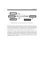
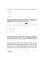
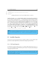
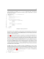
Figure 1.1 illustrates the necessary input to the binary instrumenter, and what is achieved
by it. There is the configurable binary instrumenter executable itself, which requires two
types of specification files: the adapter specification and the filer specification. Together
with a target binary, and possibly a measurement library, that results in a modified binary.
The adapter specification contains a description of the code that is inserted into the binary,
including new libraries and a tool dependent filter. The filter specification is intended to be
modified by the user to limit or in general select the scope of the instrumentation. Any filter
file can contain more than one filter, which of them to invoke is passed to the instrumenter
using command line arguments.
The current platform support is limited to the x86 and x86 64 platform due to Dyninst’s
current status. More on other restrictions can be found in 7.
1
6
Introduction
Adapter Specification
Filter Specification
Target Binary
Generic Instrumenter
Instrumented Binary
Measurement Library
Figure 1.1: Input to and output of the generic binary instrumenter.
The instrumenter itself reads from the adapter specification the defined code, stores it internally in an intermediate representation and converts it later to a Dyninst Snippet that will
be inserted into the target binary. On a per filter basis the user can select the appropriate
code to insert at the selected points of instrumentation. If more than one filter is used, the
instrumented takes care of not to insert the same code twice at a particular location.
Any filter follows the idea of starting with a base set of functions, currently none or all,
and from there on to either include or exclude functions according to specified criteria.
The resulting set of functions will then be instrumented, with loops and callsites checked
for additional requirements as they are defined. Thus one first limits the scope where to
instrument at all, and then defines what to instrument how within that scope. For example
to target callsites to foo() only in bar() one would limit instrumentation in general to bar(),
and require the callsite to call foo();
7
Chapter 2
Build Instructions
The following libraries are necessary to build the configurable binary instrumenter: XercesC and Boost are directly required by the configurable binary instrumenter, while LibElf,
LibDwarf and NASM are required by Dyninst, depending on the used platform (see Dyninst
Manual for more). The build is known to work with GCC 4.3+ (Intel x86/x86 64) and GCC
4.1 on Jugene(BlueGene/P). In the following sections, the build commands as they were
used on JUROPA are described to provide an overview.
Additionally we provide one archive that includes all the dependencies you may need,
including a build script that should work with little to no changes (see Section 2.7).
Prerequisite to those libraries especially mentioned is the availability of libiberty(binutils-dev
package) and libxml2(libxml2-dev).
2.1
XML Parser: Xerces-C
The Apache Xerces Library can be found at: Apache Xerces1
1
2
3
./configure --prefix=$HOME/xerces3
make
make install
Listing 2.1: Build Xerces C
1 http://xerces.apache.org/xerces-c/
2
8
2.2
Build Instructions
Libelf
The LibElf can be found at: LibElf 0.8.132
1
2
3
./configure --prefix=$HOME/libelf
make
make install
Listing 2.2: Build Libelf
2.3
Libdwarf
The LibDwarf can be found at: LibDwarf3
1
2
3
4
5
6
7
8
9
10
11
export CFLAGS="-I$HOME/libelf/include -fPIC"
export CPPFLAGS="-I$HOME/libelf/include -fPIC"
./configure \
--prefix=$HOME/libdwarf \
--includedir=$HOME/libelf/include \
--libdir=$HOME/libelf/lib \
--enable-shared
make
cp libdwarf.so libdwarf.h dwarf.h libdwarf.a $HOME/libdwarf
Listing 2.3: Build Libdwarf
2.4
1
2
3
Nasm
./configure --prefix=$HOME/nasm
make
make install
Listing 2.4: Build NASM
1
export PATH=$PATH:$HOME/nasm/bin
Listing 2.5: Add NASM to PATH
2.5
Dyninst
2 http://www.mr511.de/software/english.html
3 http://reality.sgiweb.org/davea/
2.6
1
2
3
4
5
6
7
8
Boost
9
export LDFLAGS="-L$HOME/libdwarf -L$HOME/libelf/lib"
./configure \
--prefix=$HOME/dyninstAPI \
--with-libdwarf-incdir=$HOME/libdwarf \
--with-libdwarf-libdir=$HOME/libdwarf \
--with-libelf-incdir=$HOME/libelf/include \
--with-libelf-libdir=$HOME/libelf/lib
Listing 2.6: Build Dyninst
2.6
Boost
You need not to build every boost library as the instrumenter only needs program options
and regex, but the easiest way of building boost is to just build everything, as shown here:
1
2
3
./bootstrap.sh --prefix=$HOME/boost
./bjam
./bjam install
Listing 2.7: Build Boost with libraries
2.7
Dependency Package
The cobi package includes LibDwarf, LibElf, Xerces-C, Boost 1.44, and Dyninst 6.1. After
unpacking the tarball cobi.tar execute install.sh, check that the shown install directory is ok and then wait for the build to finish. This may take a moment, especially building
boost consumes quite some time.
The libraries we do not include are libiberty and libxml2. If you do not have those installed
please do so. The library libiberty is often located in the binutils-dev package.
2.8
The Configurable Binary Instrumenter
To build the instrumenter, modify the Makeinstrumenter.conf file and if necessary
Makeinstrumenter, too. The .conf file includes all variables that need to be set for
building the instrumenter. They should match the paths and names to the libraries mentioned in the previous sections.
If you use the package including the dependecies you will at the end be asked whether to
continue building cobi, you do not have to change anything in that case. If not you may
have to change the DEPSBASE variable in makeinstrumenter.conf.
10
2
Build Instructions
To set the Boost, Dyninst and Xerces folders and library names, change the next few lines
in the .conf file.
Then execute the all target using:
make -f Makeinstrumenter all
If interested run make test, which should produce an output that in the first part produces only ok and the generates some text tree consisting of syntax nodes. However, this
test only verifies that the code parser for the adapter specification works as desired.
If you run into problems during linking, the target onlylink tries to relink the instrumenter without building all object files.
For more tests or examples, including binaries to modify and a newly added library, go
to the test directory, where you can invoke make and make instrument to produce a set
of m_* binaries that should work, assuming that you have set the appropriate paths in
LD LIBRARY PATH.
LD LIBRARY PATH must include paths to libDwarf, libElf, and the Dyninst library folder.
11
Chapter 3
How-to Invoke the Instrumenter
Once you have build the instrumenter and have your target binary available, the next step
is to execute the binary instrumenter. If you already have filter and adapter specification,
and to tell it via the command-line parameters which filters to evaluate, which adapter
specification to utilize and which target binary to modify. How-to define both, the adapter
specification and the filter specification, will be covered in the next two chapters. We assume for the normal usage that an adapter specification is supplied by the used measurement system which has not to be modified.
An example call would look like:
cobi -f myfilter.xml -a scalasca.xml --use all --bin myapp --out inst_myapp
To tell the instrumenter which filter specification file to use, specify the --filters parameter (-f). Analog specify the --adapter parameter (-a) to select an adapter specification
file. Using --bin (-b) allows to name the binary which will be modified. If no --out is
specified, the --bin value will be prepended with instr_ to create the name of the newly
instrumented binary. Otherwise --out names the modified executable.
All options besides --filter, --adapter, and --bin are optional.
1
2
3
4
5
6
7
8
9
10
11
12
13
14
15
16
Available Options:
Input and Output files:
-f [ --filters ] arg
-a [ --adapter ] arg
-b [ --bin ] arg
-o [ --out ] arg
--use arg
filter file to use
adapter file to use
binary to modify
output file
use named filter (default use all filters in
specified file)
--report arg
file name html report/browser
--scalasca-filter arg
filter file with functions instrumented
--not-scalasca-filter arg filter file with functions not instrumented
--id-list-file arg
file where to store ids with the region name
--tpl-filter arg
write template filter to file specified
--tpl-adapter arg
write template adapter to file specified
12
17
18
19
20
21
22
23
24
25
26
27
Flags:
--help
--preview
--test
--ignore-noentry
--ignore-noexit
--show-ipaddress
--list-all-properties
--with-dependencies
--show-timings
3
How-to Invoke the Instrumenter
lists available options
no instrumentation done, just show results of filter
and produce report if specified
run parser tests and exit
instrument functions with no entry
instrument functions with no exit
show instrumentation point addresses of functions
list all properties that are supported
open all dependency libraries for instrumentation
show where instrumenter spends its time
Listing 3.1: Command-line Parameters
The --use command is optional. If provided, it limits the filters evaluated to those specified. It takes a list in the form of colon separated filter names, e.g. filter1,filter3. If no filter
is specified, all filters contained in the file are evaluated and the instrumentation inserted
accordingly.
If you want to start your filter or adapter specification almost from scratch, you may choose
to start with the --tpl-filter or --tpl-adapter and create files that already contain
the necessary elements.
13
Chapter 4
The Adapter Specification
As mentioned earlier, the adapter specification is an XML document, containing multiple
elements to define the following:
• List of libraries to add
• An adapter filter to remove, e.g., the measurement system
• One or multiple code defining elements
The adapter specification separates the code definition from the filter definition, because
the adapter spec is expected to be constant and delivered alongside the measurement system, whereas the filter spec will be changed by the user. Listing 4.1 provides a simple
example of the three top elements defined within the adapter root element.
1
2
3
4
5
6
7
8
9
10
11
<?xml version="1.0" encoding="UTF-8"?>
<adapter>
<dependencies>
</dependencies>
<adapterfilter>
</adapterfilter>
<code name="instfunctions">
</code>
</adapter>
Listing 4.1: Adapter Specification Root Elements
4
14
4.1
The Adapter Specification
Adding Additional Libraries
To use Dyninst’s ability to add additional libraries to the target binary as a dependency it is
possible to specify new libraries, for example, if the measurement system is available in a
shared library. The binary’s name has to be specified. The path where Dyninst looks for it
has to be set in the environment variable LD_LIBRARY_PATH. This assures that the library
will be found later during program startup.
To add any new library as a dependency to the binary one needs to add one new library
child element per new dependency to the dependencies element with the adapter spec.
An example is in Listing 4.2. Note: If no calls are made to the dependency library, it will
not get added!
1
2
3
4
5
6
<?xml version="1.0" encoding="UTF-8"?>
...
<dependencies>
<library name="libscalasca.so" />
</dependencies>
...
Listing 4.2: Defining new dependencies
4.2
Define an Adapter Filter
The adapter filter targets especially the removal of any functions related to the measurement system from the set of instrumentable functions. It may also be used to remove those
functions, that are known to introduce problems (see Chapter 7.2). To define an adapter
filter, specify the the adapterfilter element and refere to Chapter 5 for how to specify
the filter. The adapter filter removes any function matching the defined filter.
1
2
3
4
5
6
<?xml version="1.0" encoding="UTF-8"?>
...
<adapterfilter>
<!-- filter here -->
</adapterfilter>
...
Listing 4.3: Defining an adapter filter
4.3
Define Inserted Instrumentation Code
The code that shall be executed at the supported locations is defined inside the code element. The four supported locations in general include
4.3
Define Inserted Instrumentation Code
15
• before
• enter
• exit
• after
With regards to function instrumentation enter marks the entry of a function, and exit marks
its exit locations. Regarding loop instrumentation before will execute before the loop, enter
at the start of an iteration, exit at the end of an iteration and after executes after the loop is
done. For call sites before the call and after the call has returned.
For each location an element can be added to code, see 4.4. Within each of these elements
one can define the code to be executed using the syntax described in the next section, in
general it is similar to a subset of the C language, without some constructs. New features
in the future aim to expose most of Dyninst’s capabilities for snippet generation.
1
2
3
4
5
6
7
8
...
<code>
<before></before>
<enter></enter>
<exit></exit>
<after></after>
</code>
...
Listing 4.4: Code Element
To support measurement system requirements that include initialization and finalization
two more elements are possible: init and finalize. The specified snippets are inserted
at the entry and exit of the main() function, or the function specified by the user. The init
and finalize code is inserted once per instrumentation object, which means per instrumented
function there is one instance of the init and finalize code inserted. Analog for loops and
callsites.
In cases where different types of initialization need to be invoked in a specific order, the init
element supports a priority attribute. According to the priority, the init code is inserted at
the beginning of the target function (main()). Where the order is from a low priority value to
high priority values, thus 0 is inserted before 1. In case of the TAU toolkit this is illustrated
in tautests/adapter.xml, featuring a code definition for tau_dyninst_init() with
priority 0, and another code element inserted per instrumented function featuring an init
element with priority 1. This takes care of initializing TAU before any function is registered.
Check the filter.xml to see how the different codes are inserted.
Executing a particular function just once, e.g., to initialize the measurement system, can be
achieved by instrumenting main() or another function specifically with a call to the desired
setup routine.
4
16
4.3.1
The Adapter Specification
Accessing Context Information
We introduce a set of variables, that are enclosed in @, to allow the instrumentation to access context information regarding the instrumentation point, e.g., function or file name. A
detailed list is given in Table 4.1. However, not all of them are available at every location.
Some, like @FILE@, are only available when the binary includes the necessary debug information. The variables @1@ ... @9@ to access function call parameters are only available
at the function’s entry location. Except for the parameter access variables, all variables are
constant and inserted during instrumentation.
Variable
@ROUTINE@
@ROUTINEID@
@LOOP@
@FULLLOOP@
@LINE@
@CALLEDROUTINE@
@ID@
@INTID@
@FILE@
@1@, @2@, ...
Value
Name of function containing instr. point
Integer ID per function, continuous
Name of loop according to Dyninst’s API
Function name + _ + Loop name
Linenumber corresponding to instr. point
Name of function called at callsite
unique numeric ID as const char*
unique integer ID, for any context, non-continuous
Name of file where function is defined
function call parameters
Table 4.1
All context variables are represented by Dyninst constant expressions and thus using the
same variable in different places within one context yields the same object, i.e., compairing
the addresses of @ROUTINE@ is possible. This however is no longer true if using the .
operator to concat multiple variables.
4.3.2
Using Variables
Variables themselves are not declared within the code elements. Two types of variables
are supported: global variables and local variables. Global variables are available in each
inserted snippet, whereas the local variables are only available for all snippets related to
one code instance. A local variable for function instrumentations is shared between the
init,enter,exit, and finalize snippets, but not between the different instrumented functions.
See the Tutorial in Chapter 6 for an example that counts the number of calls per function in
a local variable.
To specify global variables use one globalvars element and specify any necessary variables with var elements below it as illustrated in Listing 4.5.
1
2
3
4
<globalvars>
<var name="i" type="int" size="4" />
<var name="j" type="int" size="4" />
</globalvars>
Listing 4.5: Global Variable Definition
4.3
Define Inserted Instrumentation Code
17
To define local variables specify an element variables inside the code element, and one
element var within it per variable, similar to the global variables.
1
2
3
4
5
6
<code name="...">
<variables>
<var name="i" type="int" size="4" />
<var name="j" type="int" size="4" />
</variables>
</code>
Listing 4.6: Global Variable Definition
The instrumenter will at first try to look up the specified type, and create a variable of that
type’s size. If the type cannot be found a variable of the specified size will be created. All
variables are static, the are reserved during instrumentation and have a constant size and
memory location, located in the binary. That especially implies that all variables in e.g.
functions are identical, contrary to normal stack variables.
4.3.3
Supported Syntax
The syntax borrows from C, and should allow the needed constructs to interact with the
target measurement system. The essential features support calling functions and passing
contextual information about the instrumentation point. Additional support is present to
assign values, do computations and express conditional behavior.
To access context information about the instrumentation point the <SOME NAME>+ is used
to access for example the function’s name surrounding the instrumentation point. A list of
possible values is given in Section 4.3.1.
Some examples of possible codes are given in Listing 4.7
1
2
3
4
5
6
7
enterFunction(@ROUTINE@);
enterLoop(@ROUTINE@." ".@LOOP@);
i = i + 1;
printNameAndCount(@ROUTINE@,i);
handle = defineRegion(@ROUTINE@,@LINE@);
printf(@ROUTINE@." ".@FILE@);
if(handle>0) { enterHandle(handle); } else { define(handle,@ROUTINE); }
Listing 4.7: Example Codes
4.3.4
Adapterspecific Settings
Different adapters need to change some settings that depend on the adapter and not on the
target application or any user input. Those settings are stored inside the adapter specification’s adaptersettings element. The available options include:
4
18
The Adapter Specification
1. <saveallfprs value="{true|false}" /> Use this property to tell the instrumenter whether to save all floating point registers before executing the instrumentation or not. Currently all measurement systems we tried need this option to be true!
2. <initfunctionname value="{main|...}" /> Use this property to change where
the initialization of the measurement system needs to be executed. The named function’s entry point will be the location of all init codes specified.
3. <finalizefunctionname value="{main|...}" /> Similar to the init function
use this property to specify where finalization shall take place. this is in general less
problematic, the end of main is in most cases sufficient.
4. <nonreturningfunctions>...</...> This list of function may be used in future to specify functions that will not return in the control flow, but are as such not
recognized by Dyninst. This can lead to a larger than necessary number of overlapping functions.
It may in general be good advice to remove the function where init code is placed using
the adapterfilter from further instrumentation, although any further instrumentation using
enter will be executed after any init code. Besides main, other valid options for init code
placement are _start or __libc_csu_init.
4.3.5
Adapter Setup and Shutdown
To support measurement systems that need some setup and shutdown code the adapter
specification features two elements that may be used to define code that will be inserted at
the beginning and end according to the adapter settings in Section 4.3.4. These elements
are shown in Listing 4.8.
1
2
3
4
5
6
7
<adapterinitialization>
// setup() here
</adapterinitialization>
<adapterfinalization>
// shutdown() here
</adapterfinalization>
Listing 4.8: An empty filter
The SCOREP adapter scoreptests/adapter.xml illustrates the usage of all the described features, including variables and measurement system setup. You may also use
cobi --tpl-adapter to get an empty adapter specification with all possible elements.
19
Chapter 5
Filter Configuration
In this chapter the filter configuration will be explained. A filter describes two things: a
set of functions resulting from applying the different filter rules and a definition of how
to instrumented the resulting set of functions. To define how to instrument the result set,
code snippets, identified by their respective names used in the adapter specification, are
referenced. The selection of functions limits the scope of the instrumentation, applying the
different types of instrumentation only within those functions selected.
Rules used for filtering are split into patterns and properties. Briefly, patterns refer to string
matching based on the function’s identifiers, such as its name or its class name. Whereas
properties expose other features of the particular function, e.g., the complexity, the number
of call sites or the location in the application’s call graph.
5.1
Available Patterns
To access the different parts of the identifier, four different pattern rules are available:
1. names
2. functionnames
3. classnames
4. namespaces
To enable the necessary flexibility there are multiple possibilities of how to match the specified patterns against the function’s identifier. Those include:
5
20
Filter Configuration
• prefix will try to match the given patterns with the start of the selected identifier. For
example the pattern f and prefix matching would select all functions starting with f,
whereas fo would select all starting with fo.
• suffix will match the last section of the identifier with the specified patterns
• find will match if the pattern occurs somewhere in the identifier
• regex will try to match the regular expression with the identifier
• specifying nothing, will try to match the complete identifier with the pattern and
check for equality
For further information about the regular expressions you may consult the Boost Regex
Manual1 which explains the supported Perl Regular Expression syntax.
There is one additional string based rule modulenames. It contains one of the following
values: the file name if debug information is available where the function was defined,
the name of a shared library if no debug information is available, or DEFAULT_MODULE. In
general excluding DEFAULT_MODULE may be excluded to target only user code.
5.2
Operators to Combine Rules
Before we introduce properties, we show you how to combine different rules. For the
purpose of building more complex rules there are three logical operators available:
<and></and>, <or></or>, and <not></not>
The Not rule negates the one rule within it. And evaluates all children, and returns true if
and only if all children are true. Or will return true if at least one of its children is true.
In some cases the value true and false may come in handy, so they are available as:
<true /> and <false />
For example they aide if one wants to disable parts of a filter for testing, although using
XML comments (<!-- -->) is possible, too.
5.3
Using Properties
There are multiple properties available allowing you to access more detailed information
about functions in general. To use an property you use the property element in the specification and specify the type using the name attribute. You can show which names are
supported by invoking cobi --list-all-properties.
1 http://www.boost.org/doc/libs/1
45 0/libs/regex/doc/html/boost regex/syntax/perl syntax.html
5.4
Creating your own filter
21
For example:
<property name="linesofcode" minValue="5" maxValue="0" />
5.4
Creating your own filter
Any filter within the specification has to be enclosed by a filter element. Each filter is
assigned a name attribute, identifying it within the filter specification. In addition it needs
two other attributes: the start attribute and the instrument attribute (see Listing 5.1).
1
2
<filter name="somename" instrument="functions=epik" start="none">
</filter>
Listing 5.1: An empty filter
The instrument attribute defines how the result set of functions, with loops and callsites,
will be instrumented by the instrumenter. Thus the filter above tells the instrumenter to instrument functions with code named epik (refer to Section 4.3). In general the instrument
attribute consists of key=value pairs separated by ",". Key is one of the three options:
functions, callsites, or loops. If the value is omited, it will be set to the key value. If code is
present that is named functions, this makes filter definition a bit shorter. The start attribute
defines whether the filter starts with all instrumentable functions or no functions.
Within a single filter element there are different child elements allowed. We will look at
them in the following order: include, exclude, loops, and callsites. A filter is a set of include and exclude elements, that are evaluated in the order specified. A filter starts with
a particular set of functions, according to the start attribute and the either includes further functions according to an include element, or excludes functions from the current set
according to the exclude element. Each include or exclude node contains one rule that
is build from smaller rules as it is explained before using logical operators, patterns, and
properties.
1
2
3
4
5
6
7
8
9
10
11
12
13
14
<filter name="mpicallpath" instrument="functions=epik" start="none">
<include>
<property name="path">
<and>
<functionnames match="prefix">MPI mpi</functionnames>
<not>
<functionnames>MPI_Wtime mpi_wtime
MPI_Comm_rank mpi_comm_rank
</functionnames>
</not>
</and>
</property>
</include>
</filter>
Listing 5.2: MPI call path filter example
5
22
Filter Configuration
Looking at the example in Listing 5.2 we see a filter that is meant to instrument MPI call
paths, with some exceptions. How is that achieved: At first we start with an empty set
(start equals none) and then continue to include functions that match the specified rule.
The topmost rule is a property, the call path property. The call path property selects functions (returns true) for functions on call paths to the set of function specified by the properties child rule (the rule defined within the property’s body). In the examples case we
build the set of all functions that start with MPI or mpi, but without MPI Wtime, mpi wtime,
MPI Comm rank, and mpi comm rank. This is achieved by combining the two rules using
the and and not operator. While this is mere an example, exclusion of those functions might
make sense as these functions may be invoked unrelated to real communication involving
two or more processes. Using the lower and upper case names may be necessary in fortran
and C/C++ cases, and serves as an example of how to list options within pattern elements.
As you are able to specify different filters to be evaluated, the instrumenter itself takes
care of only instrumenting one location with one instance of a particular code. However,
if different filters specify different codes, e.g. using functions=epik and functions=printname,
both codes would be inserted at a particular location.
Considering the example above, one may want to remove some functions due to overhead
or as one is not interested in these call trees. This can be specified by adding a exclude
element after the include and define the rule accordingly.
1
2
3
4
5
6
7
8
9
10
<filter name="mpicallpath" instrument="functions=epik" start="none">
<include>
<!-- call path here -->
</include>
<exclude>
<functionnames>
main smallfunction othersmallfunction
</functionnames>
</exclude>
</filter>
Listing 5.3: Exclude some functions
The filter as we have seen so far is used to limit function instrumentation to particular
regions. But the filter goes beyond that, more generally speaking it limits the scope of any
instrumentation to the functions returned. The supported callsite and loop instrumentation
is only applicable within the functions with those returned by the filter. To supplement this
filtering two additional elements are allowed below the filter element: callsites and
loops. So choosing the callsites and loops to instrument is a two-step process. First the
include/exclude elements limit the scope in general, an apply function instrumentation if
specified. In the next step, the rules within loops and callsites is evaluated to further
constrain which callsites and loops are instrumented.
1
2
3
4
5
6
7
<filter name="mpicallpath" instrument="loops=loop,callsites=call" start="none">
<include>
<true />
</include>
<loops onlyOuterLoops="true">
<true />
</loops>
5.5
8
9
10
11
Available Properties
23
<callsites>
<functionnames match="prefix">MPI</functionnames>
</callsites>
</filter>
Listing 5.4: Instrument outer loops and MPI callsites everywhere
For this purpose the callsite element’s filter contains a new rule, similar to include/exclude. Every callsite is then checked to verify whether the called function satisfies the rule.
If so, the callsite is instrumented. The loop element simply provides the ability to further
refine the set of functions where loop filtering should be applied. Thus out of the filter’s set
you are able to remove even more functions. However, including new ones is not possible.
The loop element is special, as it currently takes two attributes: onlyouterloops, either
true or false, to specify whether only outer loops or all loops must be instrumented and
names which can be used as following: if empty all loops are instrumented, but you may
specify a list of names separated by ",", the use of "*" is supported to filter sets. Loops
are named in a tree fashion starting with loop 1 to loop n where children of loop 1 would
become loop 1.1 to loop 1.n and so on. To select all loops below loop 1 use:
<loops names="loops_1.*"><true /></loops>
N OTE :
Both elements loops and callsites default to the false rule, thus you need to specify true
rule if you want to instrument all loops or callsites encountered within the selected functions!
5.5
Available Properties
In this section we list all properties that are currently available for usage within the filter
specification and the adapter filter (contained in the adapter specification file).
5.5.1
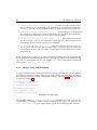
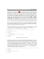
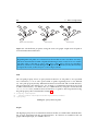
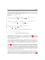
Call Graph Properties
Two different call graph related properties are available and described in the next two sections. The call graph itself is generated using static analysis via Dyninst, thus building the
call graph by reported call sites.
N OTE 1:
Static call path analysis is not able to resolve calls done through function pointers, and
as such is also not able to resolve calls using virtual functions. This may yield functions
that seem unreachable or not called.
5
24
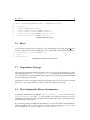
set
set
bar
foo
set
bar
update
bar
foo
foo
MPI_Send
MPI_Send
MPI_Send
MPI_Recv
compute
Filter Configuration
exchange
compute
update
exchange
doIterations
Main
Depth 1 from doIterations
MPI_Recv
MPI_Recv
compute
update
exchange
doIterations
doIterations
Main
Main
MPI call path
Forward path
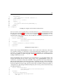
Figure 5.1: The different properties using the static call graph: Depth and call path in
forward and backward direction.
N OTE 2:
Regarding MPI call paths our evaluation has shown that in some cases there are many
functions instrumented for MPI call paths that during normal execution are not on MPI
call paths. This is often due to calls to MPI Abort or MPI finalize calls in error handling
functions, which are not called during normal operations. Therefore, it may be necessary
to inspect the result, as there may be room for improvement.
Path
The call path property allows to query functions that lie on call paths to user specified
sets of functions, or are at some point called on paths originating from a user defined
set. The path property thereby differentiates between backward and forward direction,
where backwards is the default case. For example, to instrumention functions involved
in MPI communication, one defines the set of MPI functions, using the aforementioned
functionnames rule, and then selects all functions on paths to that set particular using
the path property. This is illustrated in Listing 5.5.
1
2
3
<property name="path">
<functionnames match="prefix">MPI mpi</functionnames>
</property>
Listing 5.5: Query MPI call paths
Depth
The depth property allows to instrument all functions that are called within a defined number of steps originating from the specified function. If a function is reachable in the call
graph within depth steps, it is added to the set.
5.5
Available Properties
25
Usage:
<property name="depth" origin="doIteration" depth="1" />
5.5.2
Single Function Properties
Lines of Code
The linesofcode property uses available debug information to compute the number of
source lines between the first function entry and last function exit instrumentation point.
Specify minValue and maxValue to limit which functions are instrumented. If the maxValue
equals 0 it is ingored.
Usage:
<property name="{linesofcode|loc}" minValue="3" maxValue="0" />
Cyclomatic Complexity
The cyclomatic complexity, introduced by McCabe, analyzes the control flow graph provided by Dyninst, counting branches and basic blocks to determince the metric value. The
cyclomatic complexity can be used to identify functions where the control flow is less complex and therefore less time might be spend in the function itself.
Usage:
<property name="{mccabe|cc}" minValue="3" maxValue="0" />
Number of Instructions
The countinst property allows to decide whether or not a function shall be instrumented
base on the number of instruction used in the function. For that property we call the number of instructions Dyninst yields per basic block.
Number of Callsites
The countcallsites property accounts for the number of callsites that is present within
the function. Allowing for example to exclude leaf nodes in the call graph, function that do
not call other functions.
5
26
Filter Configuration
Number of Callees
The countcallees property yields the number of functions that call a particular function.
Has Loops
The hasloops property is true for all functions that do contain at least one loop. It supports the attribute level to require a certain nesting level of loops. Thus a level of two
would return true only for those that contain one loop with an additional loop nested
within it. Setting min- and maxValue enables a lower and upper bound for the number
of loops. Usage:
<property name="hasloop" minValue="3" maxValue="0" level="2" />
5.5.3
Miscellaneous
Has overlay?
The hasoverlay property identifies functions that are reported to shared sections of their
binary code with different functions, thus, often sharing entry and exit points. One has
to be careful to instrument these functions, as events may be wrongfully triggered. Overlay may also originate from wrongful parsing, where function entry and exit sites are not
properly detected and parsing continues beyond function borders.
N OTE :
We recommend to exclude those functions with overlay using an adapter filter if your
measurement system relies on the correct order of entry and exit events, because these
events may be triggered wrongfully if an exit is assigned to the wrong function.
Number of Exits
The countexit property enables to define limits regarding the number of exit sites. This
is most useful to exclude functions that do not have an exit point, instrumenting those may
yield wrong results as the function is entered but never exited, messing up any call tree
tracking.
Number of Entries
The countenter property is analog to the number of exits, allowing to exclude functions
depending on the number of entry sites. The instrumenter defaults to not instrumenting
5.5
Available Properties
27
functions without enter or exit sites, this however can be disabled using the proper flag.
This property combined with the number of exits, then yields access to similar behavior if
desired.
Is Library Call
This islibrarycall property identifies functions that are not within the target binary
but a library. When debug information is present in a library the modulename gets filled
with a filename, too. Therefore, it is no longer sufficient to use the module name to identify
whether a function is in a library or not, or user code or not.
Returns Float or Double
Using the returnsfloatordouble one is able to identify functions returning float or
double values. Due to the handling of floating point registers, saving and restoring them,
at function exits it may be necessary to remove those functions, although we currently
encourage the saving of all FPRs to ensure correctnes. Dyninst may in the future handle
the case of returned float or double values in a fashion that avoids any problems here.
28
5
Filter Configuration
29
Chapter 6
Tutorial
This chapter will guide you through a complete workflow of defining a filter and an adapter
that uses a small example application to show you how the instrumenter interacts with
your application. It will create one application to be instrumented, one library to provide
the measurement API, providing two functions to call for enter and exit events. On the
instrumenter side we will create the adapter and the filter file to selectively instrument two
functions in the binary to report their entry and exit.
The application and the library are C++ code shown in Listing 6.1 and Listing 6.2. Listing 6.1 shows the target application, that will be instrumented. It contains the main()
function and the foo() function, which is called in a loop. Both these functions will be
instrumented later, to register their enter and exit events.
1
2
3
4
5
6
7
8
9
10
11
12
13
14
15
16
#include <iostream>
void foo() {
std::cout << "executing foo()\n";
}
int main(int argc, char** argv) {
std::cout << "=== start main ===\n";
for(int i = 0; i < 5; ++i) {
foo();
}
std::cout << "=== finish main ===\n";
return 0;
}
Listing 6.1: Example Application (main.cpp)
Listing 6.2 illustrates a primitive measurement library. It contains three functions. The
functions enterFunction() and exitFunction() will print out the function name, file
6
30
Tutorial
name and line number if called with the appropriate values. We will call them at the function entry and exit location, respectively. The third function enterFunctionShowCount()
prints a function name and the count value passed to it. This will be used to print the number of times the foo() function is called.
1
2
3
4
5
6
7
8
9
10
11
12
13
14
15
16
#include <iostream>
void enterFunction(char* name,char* filename, int linenumber) {
std::cout << "enter: " << name << " in "
<< filename << "(" << linenumber << ")\n";
}
void exitFunction(char* name, char* filename, int linenumber) {
std::cout << "exit: " << name << " in "
<< filename << "(" << linenumber << ")\n";
}
void enterFunctionShowCount(char* name, int count) {
std::cout << "enter: " << name
<< " count: " << count << "\n";
}
Listing 6.2: Example Measurement Library (lib.cpp)
1
2
g++ -O0 -g -o app main.cpp
g++ -O0 -g -o mlib.so -shared -fPIC lib.cpp
Listing 6.3: Build application and library
To build the application and the library g++ is used, as shown in Listing 6.3. This creates
the library in mlib.so and the application to be instrumented in app. The application and
library is compiled without optimization, as this would result in static code,e.g., unrolled
loops and inlined function calls.
Now we need to create the adapter specification, which will define what code shall be executed and a filter specification that is responsible for selecting those instrumentation points
we want to instrument. We choose to instrument the main() and foo() function. Later
we will instrument foo() with a different code, that counts the number of executions.
Listing 6.4 shows the adapter specification we will use in this case. In line 4 the adapter
specification references the mlib.so library, which tells the instrumenter to add this library to the modified binary. The folder where the library is located has to be present in
LD_LIBRARY_PATH. In line 7 a new code element is defined, named funcenterexit. Using
that name, this code can later be selected from the filter specification. It defines two different code snippets inside the enter and exit elements. When instrumenting a function, this
matches to the function’s entry and exit location.
Looking at the function call in Line 8 there are three parameters enclosed by @. These are
variables to access context information of the instrumentation point. In this case we query
the function’s name, the file name where it is defined and the line it starts(see Section 4.3.1).
They are available to access context information about the instrumentation point where the
31
code is inserted, as for example @functionname@ to inquire the name of the function
where the point is located. To specify the code itself, a syntax is used similar to C, but not
featuring all possibilities.
1
2
3
4
5
6
7
8
9
10
11
12
13
14
15
16
17
<?xml version="1.0" encoding="UTF-8"?>
<adapter>
<dependencies>
<library name="mlib.so" />
</dependencies>
<code name="funcenterexit">
<enter>enterFunction(@ROUTINE@,
@FILE@,
@LINE@);
</enter>
<exit>exitFunction(@ROUTINE@,
@FILE@,
@LINE@);
</exit>
</code>
</adapter>
Listing 6.4: Adapter Specification
Now, that the code is specified, we need to prepare a filter specification that selects the
functions we want to instrument and in addition specify how the functions shall be instrumented, meaning selecting the specified funcenterexit code from the adapter specification
for function entry and exit points.
Listing 6.5 shows the filter specification. It specifies one particular filter tutorial that we
will look at in more detail. The filter is named tutorial to be identifyable. This allows you
or the user in general to tell the instrumenter which filters to evaluate, as there may be
more than one filter defined in one specification file. The start attribute defines whether
the result set is initialized with all instrumentable functions or none of them. We choose to
start with an empty set and will include the functions we want to instrument. Therefore,
line 4 shows an include element. This will add new functions to the empty set, exactly
those that match the rule specified in line 5. These functions are taken from the set of all
available instrumentable functions. Using the functionnames element, the instrumenter
compares the name of the functions to the specified names. If they match, the rule returns
true and the function itself is added.
The filter element contains one additional attribute: instrument that is used to specify
what type of instrumentation point has to be instrumented with which code. We choose
the funcenterexit code for function instrumentation, thus any selected function entry and
exit point will be instrumented according to the code defined in the adapter specification. The filter in Listing 6.5 will therefore instrument foo() and bar() with the calls
to enterName() and exitName()
1
2
3
<?xml version="1.0" encoding="UTF-8"?>
<filters>
<filter name="tutorial"
6
32
4
5
6
7
8
9
10
Tutorial
instrument="functions=funcenterexit"
start="none">
<include>
<functionnames>main foo</functionnames>
</include>
</filter>
</filters>
Listing 6.5: Example Filter Specification
With all files in one folder, the application, the library, the adapter specification and the
filter specification, we now invoke the instrumenter according to Listing 6.6. First we name
the filter and adapter specification file, then the target application and the new name of the
mutated binary. Using use we specify that the tutorial filter shall be evaluated. Omitting
the --use parameter would evaluate all filters in the specification, thus in this case would
produce the same result. However, that will most likely result in an error, that the library
could not be found. It is therefore required to add the path where the measurement library
can be found to LD LIBRARY PATH. The instrumenter and Dyninst try to find the library
in the path, similar to where the executed binary will later look for it.
1
2
3
4
5
6
7
export LD_LIBRARY_PATH=$LD_LIBRARY_PATH:$HOME/cobi/tutorial
cobi --adapter=adapter.xml \
--filter filter.xml \
--bin app \
--out instrumented_app \
--use tutorial
Listing 6.6: Execute the instrumenter
Now, you should have a working instrumented binary that gives you the proper output
when it enters main() and each time it enters foo(). To take the example a bit further
and to show you how to use variables and initialization code, it will now be extended to
count the number of times foo() is executed. To achieve this, we will define one variable
and increment it each time the function is entered and output its value at the same time.
Variables get declared inside the code element, see Listing 6.7. This variable is then accessible by all the codes defined by that code element. The variable itself is created once per
instrumented object, e.g., in the examples case there will be two variable instances, one for
function main() and one for function foo(). Thus from enter and exit you access the
same variable, but between the two functions they are not shared. We will use the init code
element (Line 11) to set the start value to 0 and in the enter element we increment it by one
before calling enterFunctionShowCount (Line 13+).
1
2
3
4
5
6
7
<?xml version="1.0" encoding="UTF-8"?>
<adapter>
<dependencies>
<library name="mlib.so" />
</dependencies>
<code name="countfuncenter">
33
8
9
10
11
12
13
14
15
16
17
<variables>
<var type="int" size="4" name="i" />
</variables>
<init> i = 0; </init>
<enter>
i = i + 1;
enterFunctionShowCount(@ROUTINE@,i);
</enter>
</code>
</adapter>
Listing 6.7: Adapter with Variable and Increment
Now, we need to create another filter to select the function foo() and instrument it with
the code seen in Listing 6.7. Such a filter is given in Listing 6.8. The instrument attribute
is changed to select the code countfuncenter and now selects only function foo. To
instrument the target binary with this code, modify the command-line parameters and use
--use tutcount instead.
1
2
3
4
5
6
7
<filter name="tutcount"
instrument="functions=countfuncenter"
start="none">
<include>
<functionnames>foo</functionnames>
</include>
</filter>
Listing 6.8: Example Filter 2
While in this example functionnames is used to refere to the name of functions, other rules
are available to restrict, e.g., namespace or classes instrumented. In addition rules, so called
properties, are available to query more than the function identifier. For example, you may
use a property path to access the call graph. Listing 6.9 illustrates how to select all functions
leading to MPI function calls.
Using the property in line 3 all functions are returned that are on call paths leading to the
functions that match the rule inside of the property. Thus, functionnames creates a set
of functions, exactly those that start with MPI or mpi, specified in line 4 by match=prefix.
The property then returns all functions that may eventually call any of those functions.
Because the instrumenter uses a call graph that is generated statically, not all call paths
must exists during execution and some may not be discovered due to function pointers or
virtual functions. Specifying both MPI and mpi may be necessary, since Fortran and C may
use different symbols.
1
2
3
4
5
6
7
<filter name="tutcount"
instrument="functions=countfuncenter"
start="none">
<include>
<property name="path">
<functionnames match="prefix">
MPI mpi
6
34
8
9
10
11
</functionnames>
</property>
</include>
</filter>
Listing 6.9: Example Filter 2
Tutorial
35
Chapter 7
Known Issues
There are currently two known issues that need to be taken into account. First one needs to
know whether the measurement system will utilize floating pointer operations. This leeds
in some cases to overridden return values in user code and therefore introduces erroneous
behavior into the application. To avoid that, Dyninst 6.1 needs to be modified and thereby
forced to always save floating point registers. Sadly, this increases the introduced overhead
significantly.
Second, when instrumenting optimized binaries that were build with Intel Compilers, a
Segmentation Fault might occur that results from an unaligned stack layout after instrumentation (Dyninst 6.1). This will be fixed in the next Dyninst release.
7.1
Static libiberty
In cases where linking tells you about an undefined reference to cplus demangle go to
Makeinstrumenter.conf and uncomment the line containing:
LIB \+=-lcommon -liberty
7.2
GCC 4.*.5
You will run into a problem with RTSignal-x86.S on GCC 4.3.5 and GCC 4.4.5 and Dyninst
6.1.
Change Makefile in dyninstAPI/src/dyninstAPI RT/x86-64-unknown-linux2.4 in Line 67:
1
2
$(ASM_OBJS_32): %_m32.o: ../src/%.S
$(CC) $(subst -m64,-m32 -march=core2,$(CFLAGS_32)) -c $< -o $@
7
36
7.3
Known Issues
Expecting const char*
Some measurement systems rely for example on the regions name to be a unique const
char* and use only the address for further operations. We did implement the @ROUTINE@
expression to satisfy that requirement, thus @ROUTINE@ will within a function always
be the same const char* expression and you may use its address. This however is not the
case for any other context variables and also not true for expressions build using the ”.”
operator for concatenation. In such a case you may need to create a variable and assign the
expression to achieve similar behavior.
37
Chapter 8
Appendix
8.1
Syntax
Using Boost::Spirit we parse the code to our internal representation and from there transform it if needed to Dyninst’s BPatch snippets. The Grammar we use to parse the adapter
specification code is approximately (where * denotes 0 to n times):
1
2
3
4
5
6
7
8
9
10
11
12
13
14
15
16
17
18
19
IDENTIFIER ::= alpha_p | ’_’ alnum_p*
FUNCPARVAR ::= "@" ( "1"..."9" ) "@"
CONTEXTVAR ::= "@" alpha_p alnum_p "@"
PARAM ::= FUNCTION | IDENTIFIER | CONSTANT | FUNCPARVAR | CONTEXTVAR
PARAMLISTE ::= ( PARAM ("," PARAM)* ) | epsilon_p
FUNCTION ::= IDENTIFIER "(" PARAMLISTE ")"
INTLITERAL ::= int_p
STRINGLITERAL ::= """ ... """
CONSANT ::= INTLITERAL | STRINGLITERAL | CONCACTCONSTSTR
EXPRESSION ::= IDENTIFIER | CONSTANT
CONCATCONSTSTR ::= ( STRINGLITERAL|CONTEXTVAR ) ( "." CONCATCONSTSTR )*
TERM ::= ( "(" TERM ")" ( "+" | "-" | "*" | "/" ) "(" TERM ")" ) |
( FUNCTION | EXPRESSION ( ("+" | "-" | "*" | "/" ) TERM )* )
ASSIGNMENT ::= IDENTIFIER "=" FUNCTION | TERM
BOOLEXPRESSION ::= FUNCTION | EXPRESSION ( "==" | "!=" | "<" | ">" ) FUNCTION | EXPRESSION
CONDITIONAL ::= "if" "(" BOOLEXPRESSION ")" "{" PROGRAM "}" ["("else" "{" PROGRAM "}"]
STATEMENT ::= CONDITIONAL | ASSIGNMENT | FUNCTION
COMMENT ::= "/*" ... "*/" | "//" ... \n
PROGRAM ::= ((STATEMENT ";")|COMMENT) (( STATEMENT ";" )|COMMENT)*
Listing 8.1: Grammar