Download Orient 3.0.1 User Manual
Transcript
Spherical Projection and Orientation Data Analysis Software Orient 3.0.1 User Manual © 1986-2015 Frederick W. Vollmer Contents iii Legal v Installation 1. 2. 1 Introduction Tutorial 1 – Quick Start 4 Data and Coordinate Systems 2.1 Data Types 2.2 Coordinate Systems 2.3 Data Entry 2.4 Spreadsheet Integration Tutorial 2 – Plotting Spreadsheet Data 2.5 Digitizing Data 7 7 7 9 9 11 13 3. Circular Plots 3.1 Scatter Plots 3.2 Circular Histograms 3.3 Frequency Polygons 3.4 Circular Mean Tutorial 3 – Circular Plots 15 15 15 17 18 19 4. Spherical Projections 4.1 Geometry of Spherical Projections 4.2 Orthographic Projection 4.3 Stereographic Projection 4.4 Equal-Area Projection 4.5 Maxima and Eigenvectors 4.6 Confidence Cones Tutorial 4 – Scatter Plots 4.7 Contouring Tutorial 5 – Contour Plots 4.8 Coordinates and Rotations Tutorial 6 – Geographic Coordinates Tutorial 7 – Rotations 4.9 Terminology of Spherical Projections 20 20 21 22 23 24 26 26 27 31 31 36 37 37 5. Kinematic Analysis Tutorial 8 – Kinematic Analysis 39 42 6. Orientation Plots 6.1 PGR Plot 45 45 i 7. Orientation Maps 7.1 Latitude, Longitude, UTM Conversion Tutorial 9 – UTM Conversion 7.2 Google and Web Maps Integration 7.3 Google Earth Integration Tutorial 10 – Web and Google Earth Integration 7.4 Orientation Fields and Domain Analysis Tutorial 11 – Domain Analysis 47 47 47 48 48 48 49 53 57 Acknowledgements References 57 History 60 ii Legal License Orient software and accompanying documentation are Copyright © 1986-2015 Frederick W. Vollmer. They come with no warrantees or guarantees of any kind. The software is free and may be downloaded and used without cost, however the author retains all rights to the source, binary code and accompanying files. It may not be redistributed or posted online. It is requested that acknowledgment and citation be given for any usage that leads to publication. This software and any related documentation are provided as is without warranty of any kind, either express or implied, including, without limitation, the implied warranties or merchantability, fitness for a particular purpose, or non-infringement. The entire risk arising out of use or performance of the software remains with you. Citation Orient is the result of countless hours of work over three decades. It is released for free in the hope that it will be useful for scientific and educational purposes. Commercial institutions should contact the author with details of the intended use. In return for free use, any significant use of the software in analyzing data or preparing diagrams must be cited in publications, presentations, reports, or other works. One or more of the following should be cited: Citation for the modified Kamb contouring method (automatic Kamb contouring on a sphere): Vollmer, F.W., 1995. C program for automatic contouring of spherical orientation data using a modified Kamb method: Computers & Geosciences, v. 21, p. 31-49. Citation for the PGR plot or automated structural domain analysis: Vollmer, F.W., 1990. An application of eigenvalue methods to structural domain analysis. Geological Society of America Bulletin, v. 102, p. 786-791. Citation for use of the Orient software: Vollmer, F.W., 2015. Orient 3: Spherical projection and orientation data analysis software. www.frederickvollmer.com. Citation for the Orient User Manual (this document): Vollmer, F.W., 2015. Orient 3: Spherical projection and orientation data analysis software user manual www.frederickvollmer.com. An acknowledgement such as, “I thank Frederick W. Vollmer for the use of his Orient software”, “Frederick W. Vollmer's Orient software was used to prepare figures”, or even “Orient was used to prepare figures”, is greatly appreciated. iii Registration Please consider registering the software, registration is free. This helps determine usage, and justify the time spent in it's upkeep. To register, send an email to [email protected] with your user name, affiliation, and usage. You will not be placed on any mailing list or contacted again, other than my response with a thank you. For example, send me an email with something like: User: Affiliation: Usage: Dr. Frederick Vollmer SUNY New Paltz, Geology Department Research on joint orientation analysis, Catskill Mountains, NY; fault kinematics in the Hudson Valley fold and thrust belt. Teaching an undergraduate structural geology course with approximately 35 students per year. If you are specific about the type of project, this can help me in developing future releases. If you are using Orient in a teaching environment, I am interested to know the course and approximate number of students. iv Installation Orient is compiled, tested, and debugged on Macintosh OS X, Windows, and Linux. Macintosh OS X 10.5 to 10.10, Windows XP, 7 and 8, and Linux distributions (testing and debugging done in Ubuntu only) should all run without problem. On Macintosh OS X, double click the disk image file (.dmg), and drag the Orient application to your Applications folder, or other desired location. If you get the App Can’t Be Opened Gatekeeper alert message when double clicking on the Orient icon, right-click (or control-click) on the icon, choose Open, and click the Open button at the next dialog warning to launch Orient. Gatekeeper in OS X 10.7 to 10.10 must be set to allow applications other than from the Mac App Store to be opened. To do so, open the System Preferences and the Security & Privacy option. Under General select Allow apps downloaded from: Anywhere. On Windows, unzip the zip file (.zip) using the Extract All option, and drag the Orient folder to any desired location. The Orient folder contains the Orient application (Orient .exe), and a “Resources” folder which is required. Make sure to entirely extract the Orient folder from the zip file, this is the most common installation problem. On Linux unpack the gzip file (.tar.gz), and copy the Orient folder to any desired location. The Orient folder contains the Orient application (orient), and a “Resources” folder which is required. An application icon (orient .png) is included in the Resources folder if desired for installation. The Example Data folder should also be copied for use in the tutorials. After installing a new version, you may wish to reset the preferences using the Restore Defaults command in the Help menu. This will clear any options that may have changed and set them to default values. The preferences are stored in the file Orient3.xml, which is located in the folder Orient in your operating system's application preferences folder. To deinstall simply delete the Orient application folder, and optionally delete the preference folder. No other files are installed on your computer. No administrative permissions are required to install Orient, and it is possible to keep a copy on a thumb drive to run on any computer. v 1. Introduction Orient is a fast, professional, easy to use spherical projection and orientation data analysis program. In 1986 Orient introduced modified Kamb contouring (automatic contouring on the sphere, Figure 1.1), PGR (Point Girdle Random) diagrams, orientation fields, and automated structural domain analysis (Vollmer, 1988, 1989, 1990, 1993, 1995). Orient 3 brings a new level of accuracy and speed, with many new tools, including interactive data analysis, coordinate conversions, digitizing, and integration with applications such as Microsoft Excel, LibreOffice, Adobe Illustrator, InkScape, and Google Earth. Orient is for plotting and analyzing orientation data, data that can be described by an axis or direction in space or, equivalently, by a position on a sphere or circle. Examples of data that are represented by unit vectors (directed) or axes (undirected) include geologic bedding planes, fault planes, fault slip directions, fold axes, paleomagnetic vectors, glacial striations, current flow directions, crystallographic axes, earthquake epicenters, cosmic ray arrival directions, comet orbital planes, positions of galaxies, whale migration paths, and the locations of objects on the Earth. Orient has been written to apply to a wide variety data types, however many examples come from structural geology, which requires extensive manipulation and analysis of orientation data. Figure 1.2 Circular frequency polygon plot of the means of two joint sets from each of 24 counties in central New York, plotted as undirected strikes (data from Parker, 1942). Figure 1.1 Lower hemisphere equal-area modified Kamb contour plot of ice crystallographic axes with contours at 10% density, an example of undirected axial data (data from Kamb, 1959). Spherical projections (Figure 1.1) are used to display three dimensional orientation data by projecting the surface of a sphere, or hemisphere, onto a plane. Lines and planes in space are considered to pass through the center of a unit sphere, so lines are represented by two diametrically opposed piercing points. Planes are represented by the great circle generated by their intersection with the sphere or, more compactly, by their normal. Spherical projections include equal-area (used for creating Schmidt nets), stereographic (used for creating Wulff nets or stereonets), and orthographic projections, these can be plotted on either upper or lower hemispheres. Point distributions are analyzed by contouring and by computing eigenvectors of 1 undirected data, or vector means of directed data. Figure 1.3 is an example of directed data plotted on both upper and lower hemispheres. Data sets and projections can be rotated about any axis in space, or to principal axes. For two-dimensional data, such as wind or current directions, circular plots and circular histograms, including equal-area and frequency polygon diagrams, can be prepared (Figure 1.2). Figure 1.3 Upper and lower hemisphere equal-area projection of directed data, magnetic remanence directions from Precambrian volcanics, with modified Kamb contours at 20% density (data from Schmidt and Embleton, 1985, in Fisher, et al., 1987). Data can be input as spherical coordinates, longitude and latitude, azimuth and altitude, declination and inclination, trend and plunge, strike and dip, or other measurements. Orient does kinematic analysis of fault data, which is represented by a plane and the direction of slip within that plane, by generating P and T kinematic axes, tangent line diagrams (Figure 1.4), and beachball plots (Figure 1.5). Spherical projections represent data orientations, but not spacial locations. Orient therefore includes orientation maps to analyze spacial distributions of orientation data, such as the location of domains of cylindrical folding in polydeformed regions (Figures 1.6 and 1.7). Orient can plot the distribution of data globally (Figure 1.8), and integrates with internet maps, like Google Maps, and with Google Earth. 2 Figure 1.4 Lower hemisphere equal-area slip tangent plot of 38 normal faults from Crete, Greece. Each data point is defined by both a plane and a directed line (data from Angilier, 1979). Figure 1.5 Lower hemisphere equal-area beachball diagram of data in Figure 1.4 showing quadrants of P shortening (red) and T extension (cyan) kinematic axes. Figure 1.6 An axial orientation field of eigenfoliation dip lines derived from 625 foliation planes, Dovrefjell mountains, Norway (data from Vollmer, 1990). Figure 1.7 PGR (Point Girdle Random) diagram showing the variations in orientation data symmetry and scatter among structural domains defined from the data in Figure 1.6. 3 Figure 1.8 Upper hemisphere equal-area projection of 14,229 earthquake epicenters (19801990), an example of directed data plotted by latitude and longitude (data from NOAA). Tutorial 1 – Quick Start Open the Orient application to display the data entry spreadsheet, the main data display area (Figure 1.9). By default, columns for ID, Station, Strike, Dip, Trend, and Plunge are displayed. The ID is an integer that should be unique for each measurement, Station is any alphanumeric string to identify the measurement (to see all available columns, select the menu command View Data Columns, these additional columns will be covered later). Measurements for planes should be entered in the strike and dip columns, and lines in the trend and plunge columns. Use the mouse to examine the icons in the toolbar, from left to right these are Open, Save As, Spherical Projection, Circular Histogram, PGR Plot, Orientation Map, and Preferences. Most of the controls in Orient have tooltips, or help hints displayed when the mouse is over the control. Click on the Spherical Projection icon to display the default Schmidt net (Figure 1.9). The toolbar icons in the spherical projection window are Save As, Find, Zoom In, Zoom Out, Zoom Fit, and Preferences. Save As will save the image to a graphics file (there is also a separate Export Vector Graphics command in the File menu for Adobe Illustrator and Inkscape compatible vector images). Begin entering numbers into the strike and dip columns, and the spherical projection will automatically update to display them. The ID number is automatically incremented, although a different number can be entered. To identify individual measurements, click on the Find (binoculars) icon in the spherical projection window. In this mode any selected data point will be highlighted in the other window, a colored bar in the spreadsheet, and a selection icon in the spherical projection window (Figure 1.10). To only display data items selected in the spreadsheet, turn on the Plot Selected option in the Graph Menu. In this case only the selected data will be displayed on the spherical projection. Turn this off before continuing the tutorial. 4 Figure 1.9 The Orient Data Window with the spreadsheet for data entry and display, and a Spherical Projection displaying the default Schmidt net Figure 1.10 Display of data in spreadsheet and spherical projection. The data point can be selected in either window, and will be highlighted in the other window. Next, open the Preferences Dialog by clicking its icon. Select the Spherical Projection option from the pulldown menu, and the Data Symbols Panel. Check the Great Circle box (Figure 1.11), and press OK. The projection will update to show great circle arcs for each of the data points. Selecting multiple rows of data in the spreadsheet will display the calculated maximum and minimum eigenvectors, and display them on the spherical projection (Figure 1.12). 5 A common calculation required for geologic data analysis is to determine the intersection between two planes, such as bedding and cleavage to find the predicted fold axis. To do this in Orient, select the two planes, the result is displayed in the status bar and plotted on the spherical projection (Figure 1.12). Finally, click on the Circular Histogram icon to display a circular histogram, or rose diagram, of the data (Figure 1.13). By default the data is displayed as undirected data, and planes are displayed by their strikes. Figure 1.11 The Orient Preferences Dialog showing spherical projection data symbol options. Figure 1.13 The projection after selecting all data points, the minimum (blue) and maximum (red) eigenvectors are displayed. Figure 1.12 The projection after checking the Great circle option. Figure 1.14 Circular histogram of the data displayed in Figure 1.7. 6 2. Data and Coordinate Systems This chapter defines the orientation data types that Orient can analyze, including specification of the angles and coordinates used to describe them. There are numerous ways of describing an orientation, including latitude, longitude, trend, inclination, strike, and others. There are also many possible coordinate reference frames, the basics are described here with more detail for those needing it in Section 4.8. The main goal of this chapter, however, is to get the user quickly started by explaining how to enter data. Often it is simplest to enter the data directly into Orient's spreadsheet, however Orient can read and write files compatible with spreadsheet software such as Microsoft Excel and LibreOffice, and, for many workers, this is a better option. Finally, Section 2.4 explains how data can be digitized from scanned images of spherical projections or maps. 2.1 Orientation Data Types Orientation data are either unit vectors, directed data, or unit axes, axial or undirected data. Current flow directions, for example, are directed, while fold axes are undirected. Plotting, contouring, and statistical analysis of these data types is different. Geometrically, data represents either lines or planes. On spherical projections planes and lines are considered to pass though the center of a unit sphere. Planes are represented by either their great circle, the intersection of the plane with the unit sphere, or by their normal (often referred to as the plane's pole). Unit vectors or axes in three dimensions can be specified by their coordinates on the surface of the unit sphere, these are the direction cosines. However, it is more common to specify just two independent angles, a horizontal angle (such as strike, trend, or azimuth) and a vertical angle (such as dip, plunge or inclination). Two dimensional data require a horizontal angle only. Available angular measures and their definitions are listed in Table 1, and discussed in Section 2.2. Orient has separate columns for lines and for planes, this allows data that contains both, such as kinematic data (Chapter 5), to be entered as well. Unused columns can be hidden if desired by opening the Data Columns Dialog from the View Menu. Angle units can be specified as either degrees (0 to 360 degrees), gradians (0 to 400 gradians), or radians (0 to 2π radians). Orient stores all numbers internally as radians, which are transparently converted to user units. This is a global preference that sets how angles are read from files and user input, and stored in files. There is no mechanism to determine this from file input, so this should only be done if all files share the same format, or to convert files from one format to another. Degrees is the default value, and will not normally need to be changed. 2.2 Coordinate Systems Orient is designed to be used with all types of orientation measurements and coordinate systems, and converts to and from user coordinates for data entry and output. The user does not normally need to be concerned about the underlying coordinate system, except in the case of rotations or selecting different geographic coordinates (Section 4.8). Orient uses a standard right-handed spherical coordinate system defined with default axes X, Y, Z = Right, Top, Up. In geologic usage these normally correspond to East, North, Up, which conforms to map coordinate systems using Easting, Northing, Elevation. Section 4.8 explains how the default coordinates can be changed to any other orientation, such as 7 global geographic (Orient has 13 standard coordinate systems, which can be modified by rotations about any axis). Spherical coordinates are specified by two angles, θ (theta) and ϕ (phi). The standard mathematical definitions are that θ is the longitude, or the counterclockwise angle from X in the XY plane, and that ϕ is the colatitude, the angle from Z. However, there are numerous ways to specify the same information with two angles, typically specified by the scientific discipline, such as geology, geography, or astronomy (e.g., Fisher et al, 1987; Mardia and Jupp, 2000). Planes are represented by their normal, or pole. Alternatively, coordinates can be specified by three direction cosines in this coordinate system, which are the coordinates of points on a unit sphere. In Orient the user can specify θ and ϕ for lines and planes according to their data or discipline (Table 1). Geographic data are generally given using longitude as the horizontal angle, the vertical angle is commonly latitude or colatitude, azimuth and altitude are used in astronomy. Geologic data, however, are typically specified using azimuths for horizontal angles, measured clockwise from North (Y), and dips or plunges for vertical angles, measured down from horizontal (the XY plane). Geologic angles are typically strike and dip for planes, or trend and plunge for lines. Orient supports all common conventions (Table 1), and converts among them. Column Header Plane θ Strike Strike left Dip direction Plane ϕ Dip Line θ Azimuth Declination Longitude Sphere Trend Line ϕ Altitude Colatitude Inclination Latitude Sphere Nadir Plunge Zenith Abbreviation strikel dipdir az dec longs alt colat inc lats Notes Horizontal orientation angle of plane Clockwise from North (Y), dip is to right along strike Clockwise from North (Y), dip is to left along strike Azimuth of dip line Vertical orientation angle of plane Angle from XY plane down toward -Z Horizontal orientation angle of line Clockwise angle from North (Y) Equal to azimuth Counterclockwise angle from X Equal to azimuth Vertical orientation angle of line Equal to latitude Angle from Z down toward XY plane Angle from XY plane down toward -Z Angle from XY plane up toward Z Angle from -Z up toward XY plane Equal to inclination Equal to colatitude Table 2.1 Column headers used to specify orientation data formats in Orient. The header or its abbreviation is used in data files to identify a column of data. A plane requires two header, such as strike and dip. A line also requires two header, such as trend and plunge. To convert between units or to set the default units for data entry, open the Data Orientation Units Dialog from the Data Menu. This will set the orientation data units entered in the spreadsheet, and will convert any preexisting values to the new format. For example, a common conversion is from strike 8 and dip, to dip and dip direction. The data will be saved in the new format. Note that data files contain the format, opening a saved file will always have the format as saved. Due to the standard use of geographic locations, typically from GPS (Global Positioning System) positioning, of data points in geology, Orient requires a distinction between two usages of latitude and longitude for data input. A geologist typically records data locations expressed as Cartesian coordinates, such as UTM (Universal Transverse Mercator), or as latitude and longitude pairs, as well as collecting orientation data at that location. Therefore it is necessary to determine whether a latitude, longitude pair is meant as the location of a data point, or if it is the data point itself. The convention adopted here is that latitude, longitude (or lat, long) refer to a data point location, and that latitude sphere, longitude sphere (or lats, longs) refer to the data point to be plotted on a spherical projection. There is, unfortunately, more than one convention for strike and dip, including two contradictory ones both called the right-hand rule (e.g., Ragan, 2009). A distinction must be made, so by default, Orient uses the convention that the dip is to the right looking along the strike (e.g., Pollard and Fletcher, 2005; Twiss and Moores, 2007). A second convention, where the dip is to the left, the thumb of the right hand points down the dip ( Barnes, 1995), is referred to in Orient as strike left (or strikel). This convention can be selected using the Data Orientation Units command. A third convention, using a dip octant (N, NE, E, SE, etc.) is automatically converted to one of the above as described in Section 2.3. Finally, dip and dip direction are another common way of giving the orientations of plane, which is also supported. 2.3 Data Entry Each data point must include a pair of angles specifying its orientation in space. The first angle is measured in a horizontal plane (θ), and the second in a vertical plane (ϕ). For typical geologic data, these are strike and dip for planes, and trend and plunge for lines. However, all common units are supported (Table 2.1). Two dimensional data require horizontal angles only. Before entering data, select the desired data format using the Data Orientation Units command. You may also wish to hide or show appropriate columns using the View Data Columns command. Separate columns are used for planes and for lines, so make sure the required columns are visible. The Type column can contain any alphanumeric identifier, for example S0 and S1 are often used in geology to designate bedding and cleavage. This is optional, but is required if multiple data types are entered in a single file. All settings, such as symbol sizes and color, are saved for each type. Additional data attributes include station identifiers, location coordinates, domains, and comments (Table 2.2). Orient does several automatic data conversions. If data is entered as a bearing with compass quadrants it is automatically converted to a numerical azimuth. Bearings are given as degrees east or west of north or south, for example, N30W will be converted to 330. A conversion is also done for planes in strike and dip, or strike left and dip, formats if a dip octant (N, NE, E, SE, S, SW, W, or NW) is given. The strike (or strike left) will be corrected if necessary. For example a strike, dip pair entered as 10, 30W will be converted to 190, 30. 2.4 Spreadsheet Integration Data entered into the Orient spreadsheet can be saved in several spreadsheet formats: tab separated values (.tsv), comma separated values (.csv), OpenDocument spreadsheet (.ods), Microsoft Excel (.xls), and Excel Open Office XLM (.xlsx). These are all compatible with most spreadsheet programs, including Microsoft Excel and LibreOffice. 9 Orient can also read all of these formats, allowing users to enter data files into Microsoft Excel, LibreOffice, or other spreadsheet software. The only requirements are that the data have a header row, consisting of headers listed in Tables 2.1 and 2.2, and that any initial comment lines start with two slashes (//). Table 2.3 gives a simple example, and Table 2.4 gives a more complete example. The simplest possible file would be a list of horizontal angles, such as trends or azimuths, for two dimensional analysis. Three dimensional analysis also requires vertical angles, such as dips or plunges. The included folder Example Data has numerous examples of compatible files. Open them in Excel or LibreOffice to examine them, they are used in the following tutorials. Column Header Abbreviation Notes ID N Integer identification number for data point Station Alphanumeric station identifier Zone Alphanumeric zone, such as UTM grid zone Easting East, X X or easting coordinate of data location Northing North, Y Y or northing coordinate of data location Elevation Z Elevation of data location Latitude lat Latitude of data location (D°, D°M', or D°M'S”) Longitude long Longitude of data location (D°, D°M', or D°M'S”) Plane θ Horizontal orientation angle of plane from Table 2.1 Plane ϕ Vertical orientation angle of plane from Table 2.1 Line θ Horizontal orientation angle of line from Table 2.1 Line ϕ Vertical orientation angle of line from Table 2.1 Type Alphanumeric data type, such as S0 or S1 Label Alphanumeric label Domain Integer identification number for domain Comment Alphanumeric comment Table 2.2 Column headers used to specify data attributes in Orient. The header or its abbreviation is used in data files to identify a column of data. See Table 2.1 for orientation data angles. Strike Dip 230 24 018 54 141 15 Table 2.3 Example of a simple Orient data file as displayed in a spreadsheet, such as Microsoft Excel or LibreOffice, with strikes and dips of planes. See Tables 2.1 and 2.2 for other possible column headers. 10 // Example of an Orient 3 data file in a spreadsheet, this is a file comment, 2015-05-04 Easting Northing Strike Dip Trend Plunge Type Comment 8452.05 12885.05 230 24 S0 approximate 8456.03 12825.03 018 54 S0 overturned 8432.12 12922.30 141 15 S1 spaced 8466.08 12865.40 138 02 L 8492.01 12872.00 140 09 L Table 2.4 Example of a more complex Orient data file as displayed in a spreadsheet, such as Microsoft Excel or LibreOffice, with an initial file comment, data locations, multiple data types, and data comments. See Tables 2.1 and 2.2 for other possible column headers. Tutorial 2 – Plotting Spreadsheet Data Open a spreadsheet program, such as LibreOffice or Microsoft Excel, and enter the data shown in Table 2.5. // My Orientation data file Strike Dip Trend Plunge 060 65 S0 10 45 S0 40 60 S0 310 60 S0 280 70 S0 90 330 40 55 Type FH S1 Table 2.5 Example of an Orient data file for Tutorial 2. Enter this into a spreadsheet such as LibreOffice or Microsoft Excel. Save the file using a standard format (.csv, .tsv, .ods, .xls, or .xlsx) as Tutorial 2. Open the file in Orient using the Open icon, or File Open command. Press the Spherical Projection icon, and you should get a plot as in Figure 2.1. If you have previously modified settings, however, they will still be in effect. The Help Restore Defaults command can be used to reset all settings to default. 11 Figure 2.1 Lower hemisphere equal-area projection of Tutorial 2 data from Table 2.5. Figure 2.2 Equal-area scatter plot as in Figure 2.1 after removing the Schmidt net, and assigning colors to the data symbols. To prepare the plot for presentation, it is good to simplify it and focus on the data, so change some of the settings as follows. From the spherical projection window, press the Preferences icon. Under Spherical Projection in the Net pane, turn off both Net and Axes. Press Preview to see the result. In the Labels pane, set the Increment to -90, the Offset to 14, and the Size to 12. Next, assign different colors to the data types. In the Symbols pane select data type S0 (bedding), click on the data symbol icon, and assign the Fill Color blue. Select data type S1 (cleavage) and assign its fill color to green, and FH (a fold hinge) yellow. Press Preview, and the plot should be as shown in Figure 2.2. Now add great circles to represent the planes. In the Symbols pane select data type S0 again and check the Great circle box. Then select data type S1, check the Great circle box, and set the Stroke Color to green (Figure 2.3). A plot of planes represented by their great circles is a β (beta) diagram. With a lot of data this type of diagram becomes crowded, and loses any statistical significance, but for a small number of points it can help with visualization. A plot with planes represented by their poles is a π (pi) diagram, or S-pole diagram, and is preferred over a β diagram as a better statistical representation. 12 Figure 2.4 Equal-area plot as in Figure 2.3 with best-fit great circle and pole given by the minimum eigenvector of S0 (bedding). Figure 2.3 Equal-area plot as in Figure 2.2 with planes represented as great circles. Finally, add the S0 maxima. In the Maxima pane select the S0 data type, and check Visible. For this plot just add the Minimum eigenvector, which gives us a best-fit fold axis. Uncheck the Symbol for both the Maximum and Intermediate eigenvectors. For the Minimum eigenvector check the Symbol and Great circle checkboxes, and set their colors to red (Figure 2.4). 2.5 Digitizing Data When digital data files or text listings of orientation data are not available, data can be digitized from scanned images of spherical projections or maps. To digitize a spherical projection from a suitable source image, insure that the image is undistorted, that is circular, and that the north point is unrotated. An image editing program such as Adobe Photoshop or GIMP can remove distortion and rotate the image if necessary. Open the image in Orient using the File Open Image command, which will display the Digitizing Window (Figure 2.5). File types .tiff, .jpg, .png, and .bmp files are supported. Click on the Digitize icon to display the Digitize Dialog (Figure 2.6). Select the correct options for the spherical projection, the projection options are stereographic, equal-area, or orthographic, in either upper- or lower-hemisphere (one hopes that the original author correctly specified these). Select the data type, line or plane, and press OK. A prompt will ask for three points on the perimeter of the projection, after entering these, a circle will be drawn over the projection. If the circle is a reasonable fit, proceed to digitize the points, which will appear in the Data Window spreadsheet. If not, the circle can be reinitialized, or distortion of the image may need to be removed. Spurious data points can be deleted in the spreadsheet as necessary. If digitizing needs to be interrupted, save the file and reopen the file and image later to resume. To change data type, lines or planes, reopen the Digitize Dialog, select the desired one, press enter, and continue digitizing. 13 Digitizing orientation data from a map is similar. Make sure the image is undistorted, and that the X and Y directions are orthogonal with north to the top. The X and Y coordinate scales do not need to be equal, but they must each be scaled linearly within the map area. If necessary, remove any distortion using an image editor. Select Map as the source, the correct element, line or plane, and press OK. There will be a prompt for two points with known coordinates to define the area and coordinates. If the result is satisfactory, begin digitizing the elements by clicking on a start point and then an end point. The coordinates entered into the spreadsheet will be the center point between the two points. Figure 2.6 The Digitize Dialog showing options for digitizing orientation data from images. Figure 2.5 An image of a spherical projection opened in the Digitize Window. 14 3. Circular Plots Circular plots for two dimensional orientation data include scatter plots, circular histograms, and circular frequency polygons (Davis 1985; Fisher et al. 1987; Cheeney, 1983; Howarth, 1999; Mardia and Jupp, 2000). Circular plots can also be used to display the horizontal angles of lines and planes, such as lineation trends. For planes it is possible to plot the strike direction, dip direction, or the azimuth of the plane normal. The data may be directed or undirected. Undirected data plots two points at 180°, or can be plotted on a double angle, modulo 180°, plot. The settings for these plots are in the Orient Preferences Dialog using the Circular Histogram selection. 3.1 Circular Scatter Plots A simple circular scatter plot shows the data distribution on a circular plot, normally the perimeter of a unit circle (Cheeney, 1983; Mardia and Jupp, 2000). Directional rays may be drawn from the circle center, or symbols plotted on the perimeter. The vector mean, for directed or undirected data (Section 3.4), can also be displayed. There are many variations on scatter plots, Orient implements ray plots with lines drawn from the center, and with symbols on the perimeter (Figures 3.1 and 3.2). Figure 3.1 is a circular scatter plot of the orientations of 76 turtles after laying eggs (data from Gould cited in Mardia and Jupp, 2000), an example of directed circular orientation data. In order to better visualize overlapping data points, the opacity of the data point symbols is set to 50%. Figure 3.2 is a plot of the means of two joint sets from each of 24 counties in central New York (data from Parker, 1942). This data is plotted as strike azimuths, an example of undirected data. Figure 3.1 Circular scatter plot of the orientations of 76 turtles after laying eggs (Gould's data from Mardia and Jupp, 2000). 3.2 Figure 3.2 Circular scatter plot of the means of two joint sets from each of 24 counties in central New York (data from Parker, 1942). Circular Histograms Two dimensional orientation data is commonly displayed as a circular frequency histogram, where the data count is tallied for bins or sectors of a set angular width. A commonly used graph is a rose 15 diagram constructed with sector radii proportional to class frequency, an equidistance rose diagram. Figure 3.3 shows an example for directed data. Unfortunately, such a diagram is biased, and not a true histogram, because the area displayed for a single count increases with the radius. An unbiased plot is an equal-area circular histogram where each count has an equal area, and the sector area is proportional to class frequency (Cheeney, 1983; Mardia and Jupp, 2000; Figure 3.4). Figures 3.5 and 3.6 are examples for undirected data. Figure 3.4 Equal-area circular histogram, or rose diagram, of the directed turtle data shown in Figure 3.1. Each count has an equal area, removing area bias. Figure 3.3 Equidistance rose diagram of the directed turtle data shown in Figure 3.1. The increasing area for larger bin counts results in an area bias, so this is not a true histogram. Figure 3.5 Equidistance rose diagram of the undirected joint data shown in Figure 3.2. The increasing area for larger bin counts results in an area bias, so this is not a true histogram. Figure 3.6 Equal-area circular histogram of the undirected joint data shown in Figure 3.2. Each count has an equal area, removing area bias. 16 Each of these plots is drawn with 24 bins, or 15° sectors. The selection of bin size will change the appearance of the diagram, an example is shown for circular frequency polygons in Section 3.3. 3.3 Circular Frequency Polygons A circular frequency polygon (Howarth, 1999), or kite diagram (Davis, 1986), is an alternative graph for displaying the circular orientation data. In a circular frequency polygon diagram the bin sector centers are connected by straight lines to form a polygon. Figure 3.5 is a circular frequency polygon diagram of the directed turtle data (Figure 3.1) using 24 15° bin sectors, the same size as in Figures 3.3 to 3.6. Figure 3. 7 Circular frequency polygon plot, or kite diagram, of the directed turtle data shown in Figure 3.1, using 24 15° Figure 3.8 is an example of an undirected circular frequency polygon using the joint data (Figure 3.2), also using 24 15° bins. To illustrate the effect of bin size on circular histograms, Figure 3.8 is the same data plotted using 12 30° bins. 17 Figure 3.9 Circular frequency polygon diagram of the joint data as in Figure 3.8, but using 12 30° sector bins. Figure 3.8 Circular frequency polygon plot, or kite diagram, of the undirected joint data shown in Figure 3.2, using 24 15° sector bins. 3.4 Circular Mean A simple measure of location, or best-fit, to circular orientation data is the mean direction, which is calculated as a vector sum. For directed data the two sums are calculated: Then the mean resultant length and direction, or center of mass of the coordinates, is calculated as: Since the mean resultant length approaches 1 as orientations converge, it is common to cite the sample circular variance: which is 0 when all the orientations are identical. For undirected data the same calculation is done, however θ is doubled prior to the summation, and the result is halved. For details of statistical measures 18 and tests for circular orientation data see Mardia (1972), Cheeney (1983), Davis (1985), Fisher et al. (1987), and Mardia and Jupp (2000). Tutorial 3 – Circular Plots Open the file Gould from the Example Data folder (any of the .csv, .tsv. .ods, .xls, or .xlsx versions is fine) in Orient, and click on the Circular Histogram icon. If no settings have been previously modified the projection will look as in Figure 3.4. The Help Restore Defaults command can be used to reset the preferences if desired. This is an example of directed circular orientation data. The default display is an equal-area circular histogram, or rose diagram. In the Circular Histogram Symbol pane this data type is displayed as Default, as none was specified in the file. Check Directed so this data will be treated as unit vectors, instead of axes. Next, in the Histogram pane, select the Equidistance plot (Figure 3.4), and then the Frequency polygon (Figure 3.5) to compare plot types. Next, open the file Parker 1942. This is an example of undirected circular orientation data. They are treated as circular (instead of spherical) data because, although joints are planar, only the strikes were reported. Note that, because these are planes recorded by strike, the direction plotted should be specified as Strike, otherwise the plane's normal would be plotted. Reset the Histogram to equal-area. There are two data types in this file, J1 and J2. In the Symbols pane, select J1 and set the Histogram Fill Color to red, and uncheck Symbol for both data types, J1 and J2, and uncheck Directed. The resulting plot should be as in Figure 3.5. Next, in the Histogram pane, select the Equidistant plot (Figure 3.6), and then the Frequency polygon (Figure 3.8) to compare plot types. 19 4. Spherical Projections A primary function of Orient is the creation and manipulation of spherical projections of orientation data, in particular azimuthal spherical projections that project the surface of a sphere onto a plane. This chapter discusses mathematical concepts related to spherical projections, in particular the geometry of several common projections, and the spherical nets which are commonly used to display and work with these projections. A final section on nomenclature discuses terminology and common errors that occur in the literature. 4.1 Geometry of Spherical Projections A spherical projection is a mathematical transformation that maps points on the surface of a sphere to points on another surface, commonly a plane. Astronomers, cartographers, geologists, and others have devised numerous such projections over thousands of years, however two, the stereographic projection and the equal-area projection, are particularly useful for displaying the angular relationships among lines and planes in three-dimensional space. A third projection, the orthographic projection, is less commonly used, but is important for some applications, and is easily visualized. These are azimuthal spherical projections, projections of a sphere onto a plane that preserve the directions (azimuths) of lines passing through the center of the projection. This is an important characteristic as azimuths, or horizontal angles from north (strike, trend, etc.), are standard measurements in structural geology, geophysics, and other scientific disciplines. The orientations of lines and planes in space are fundamental measurements in structural geology. Since planes can be uniquely defined by the orientation of the plane's pole, or normal, it is sufficient to describe the orientation of a line. If only the orientation of a line, and not it's position, is being considered, it can be described in reference to a unit sphere, of radius, R = 1. A right-handed cartesian coordinate system is defined with zero at the center of the sphere. A standard convention, used here, is to select X, Y, Z = East, North, Up (see Section 4.8 for alternative conventions). A line, L, passing through the center of the sphere, the origin, will pierce the sphere at two diametrically opposed points (Figure 4.1). If the line represents undirected axial data (as opposed to directed data), such as a fold axis or the pole to a joint plane, it is allowable to choose either point. In structural geology the convention is to choose the point on the lower hemisphere, P (the opposite convention is used in mineralogy). The three coordinates of point P are known as direction cosines, and uniquely define the orientation of the line. More commonly, the trend (azimuth or declination) and plunge (inclination) of the line are given. In Figure 4.1, the trend of the line is 090°, and it's plunge is δ. It is a helpful reminder to designate horizontal angles using three digits, where 000° = north, 090° = east, 180° = south, etc., and to specify vertical angles using two digits, from horizontal, 00°, to vertical, 90°. Note that directed data, such as fault slip directions, may have negative, upward directed, inclinations. An important tool for plotting line and plane data by hand, and for geometric problem solving, is a spherical net. A spherical net is a grid formed by the projection of great and small circles, equivalent to lines of longitude and latitude. Nets are commonly either meridianal or polar, that is, projected onto a meridian (often the equator) or a pole. The terms equator and pole (or axis) will be used to refer to the equivalent geometric features on the net, it is essential to remember that they do not have an absolute reference frame, that is, the net axis is not equivalent to geographic north. When used to plot data by 20 hand, an overlay with an absolute geographic reference frame (North, East, South, etc.) is used (Ragan 2009). The projections described here are spherical projections, so equal-area projection is assumed to mean equal-area spherical projection. Other projections are possible, such as hyperboloidal projections, which include equal-area and stereographic hyperboloidal projections (Yamaji, 2008; Vollmer, 2011). In these projections the surface of a hyperboloid is projected onto a plane. These are used in the context of strain analysis, and are unlikely to be confused with the more common spherical projections. Figure 4.1 Definition of the point, P, on the unit sphere that defines the orientation of the undirected line L. The line is trending toward X (east) and it's plunge is δ. The Y coordinate axis (north) is into the page. 4.2 Orthographic Projection The orthographic projection is an important projection in which points are projected along parallel rays, as if illuminated by an infinitely distant light source. Figure 4.2 gives the geometric definition of the orthographic spherical projection. A corresponding orthographic polar net is shown in Figure 4.3, and an orthographic meridianal net in Figure 4.4. The projection of point P in the sphere to point P' on the plane is parallel to the Cartesian axis Z, effectively giving a projection following a ray from Z equals positive infinity. This type of projection gives a realistic view of a distant sphere, such as the moon viewed from Earth. It is azimuthal, but angles and area are not generally preserved. When plotting geologic data it is important that area, and therefore data densities, are preserved, so the orthographic projection unsuitable for such purposes. The net does, however, have other uses, such as the construction of block diagrams (e.g., Ragan, 2009). 21 Figure 4.2 Geometric definition of the orthographic spherical projection. Point P on the sphere is projected to point P' on the plane. 4.3 Figure 4.3 Polar orthographic net. Figure 4.4 Meridianal orthographic net. Stereographic Projection The stereographic or equal-angle spherical projection is widely used in mineralogy and structural geology. It is defined geometrically by a ray passing from a point on the sphere (here Z = 1) through a point P on the sphere to the projected point P' on the plane (Figure 4.5). The corresponding stereographic nets are shown in Figures 4.6 and 4.7. Both hemispheres can be represented on the net, however the convention in structural geology is to use the lower hemisphere. The meridinal stereographic net is known as a stereonet (Bucher, 1944), or Wulff net, named after the crystallographer G.V. Wulff who published the first stereographic net in 1902 (Whitten, 1966). The stereonet is commonly used in mineralogy, however, the convention is to use the upper hemisphere. It is therefore good practice to clearly label all projections, for example lower-hemisphere stereographic projection. Figure 4.5 Geometric definition of the stereographic projection. Point P on the sphere is projected to point P' on the plane. Figure 4.6 Polar stereographic net. Figure 4.7 Meridianal stereographic net, also known as a stereonet or Wulff net. The projection is azimuthal, so lines passing through the center of the projection have true direction, these represent great circles. Note that area in Figures 4.6 and 4.7 is clearly distorted, the projection preserves angles (is conformal), but it does not preserve area. An important consequence is that great circles (such as meridians) and small circles project as circular arcs. These properties make it useful for 22 numerous geometric constructions in structural geology (Bucher, 1944; Phillips, 1954; Badgley, 1959; Lisle and Leyshorn, 2004; Ragan, 2009). The distortion of area, however, makes the stereographic projection unsuitable for studying rock fabrics, such as multiple orientations of bedding, joints, and crystallographic fabrics. Plotting such data is a descriptive statistical procedure intended to identify significant clusters, girdles, and other patterns. Figure 4.8 is a lower-hemisphere stereographic projection of two data clusters which are identical except for rotation. They have identical densities on the sphere, but this is distorted on the stereographic projection. An equal-area projection (Figure 4.9) should be used instead (Schmidt, 1925; Sander, 1948, 1950, 1970; Phillips, 1954; Badgley, 1959; Turner and Weiss, 1963; Whitten, 1966; Ramsay, 1967; Hobbs et al., 1976; Fisher et al., 1987; Van der Pluijm and Marshak, 2004; Pollard and Fletcher, 2005; Twiss and Moores, 2007; Ragan, 2009; Fossen, 2015). Figure 4.8 Lower-hemisphere stereographic projection of two data clusters showing density distortion. See text for discussion. 4.4 Figure 4.9 Lower hemisphere equal-area projection of two data clusters showing lack of density distortion. Equal-Area Spherical Projection The Lambert azimuthal equal-area spherical projection is the correct projection to use for displaying orientation data. It is not conformal, but an important characteristic is that it preserves area, so densities are not distorted (Figure 4.9). As discussed in the previous section, this makes it useful for the examination of rock fabrics, including the orientations of bedding, joints, and crystallographic fabrics (Schmidt, 1925; Sander, 1948, 1950, 1970; Phillips, 1954; Badgley, 1959; Turner and Weiss, 1963; Whitten, 1966; Ramsay, 1967; Hobbs et al., 1976; Fisher et al., 1987; Van der Pluijm and Marshak, 2004; Pollard and Fletcher, 2005; Twiss and Moores, 2007; Ragan, 2009; Fossen, 2015). It appears widely in the geologic literature, and is the most likely of these projections to be encountered in scientific literature related to structural geology. Figures 4.10, 4.11 and 4.12 illustrate the geometric definition, polar net, and meridianal net respectively. The term azimuthal indicates that, like stereographic and orthographic projections, lines passing through the center have true direction, and that it is projected onto a plane. This distinguishes it from other equal-area projections, which include the projection of a sphere onto conical and other surfaces, 23 however, in structural geology, it can usually be referred to simply as an equal-area projection without ambiguity. The projection is also known as the Schmidt projection, after W. Schmidt who first used it in structural geology in 1925 (Schmidt, 1925; Turner and Weiss, 1963), and the meridianal equal-area net, is known as a Schmidt net (Knopf and Ingerson, 1938; Billings, 1942; Sander, 1948, 1950, 1970). Figure 4.10 Geometric definition of the equal-area projection. Figure 4.11 Polar equal-area net, or Billings net. Figure 4.12 Meridianal equalarea net, or Schmidt net. The Schmidt net (Figure 4.12) is not a stereonet (Figure 4.6). Stereonets are widely used in mineralogy, and their equal-angle property makes them useful for certain graphical constructions, such as drill hole problems (Ragan, 2009), however they should not be used to plot orientation data. The procedures for most geometric constructions commonly used in structural geology are identical on stereonets and Schmidt nets. Schmidt nets are required for unbiased data analysis, and can also be used to solve most common geometric problems. 4.5 Maxima and Eigenvectors Spherical orientation data is characterized by either directed unit vectors or undirected axes in space. The concept of a mean value is familiar when dealing with scalar values like temperature. Determining such a value for orientation data is more complex, averaging trends and plunges separately does not work. As with circular data, a useful measure is the vector mean, the center of mass for directed data. The procedure for finding the mean is similar to that for directed circular data. A data point on a unit sphere can be represented by three coordinates, which are its direction cosines. If we designate this point as the vector x = (x1, x2, x3), then the mean vector is the averaged sum: with mean resultant length: and mean direction, the normalized mean vector: 24 Axial data requires the computation of eigenvectors, an important concept that gives best-fit values, or moments of inertia, for tensors, such as the principal stresses of a stress tensor. In the context of orientation data, imagine that each line passing through the center of the unit sphere is represented by a small mass at each of the two points where it pierces the sphere. If the sphere were spinning, it would have a tendency to spin about the axis of minimum density, this is the minimum eigenvector. If it were rolling, it would have a tendency to stop with the maximum density at the bottom, this is the maximum eigenvector, the intermediate eigenvector is exactly 90° from the other two. As an example, Figure 4.13 is a lower hemisphere equal-area scatter plot of bedding plane normals represented by points on the lower hemisphere. The orientation tensor, or scatter matrix (Mardia and Jupp, 2000), is given by: the averaged sum of the unit orientation vectors times their transpose. The eigenvectors of this matrix are determined and plotted. In Figure 4.14 the maximum eigenvector is a red circle, the intermediate green, and the minimum blue. In cylindrical folds the minimum eigenvector of poles to bedding gives the fold axis, and a great circle drawn perpendicular to the minimum eigenvector gives the best-fit through the plane poles (Figure 4.14). Figure 4.13 Lower hemisphere equal-area projection, or scatter plot, of 56 poles to bedding in graywacke, Albany County, New York (data from Vollmer, 1981). Figure 4.14 Projection of data as in Figure 4.13, with maximum (red), intermediate (green), minimum (blue) eigenvectors, and great circle to the minimum eigenvector. For details of statistical measures and tests for spherical orientation data see Mardia (1972), Cheeney (1983), Davis (1985), Fisher et al. (1987), and Mardia and Jupp (2000). 25 4.6 Confidence Cones There are a number of models for distributions of spherical orientation data (Mardia, 1972; Fisher et al., 1987; and Mardia and Jupp, 2000). By analogy, the Gaussian, or normal, distribution is a familiar model for scalar data. Using these models, confidence cones can be drawn around either the mean direction, or the eigenvectors (Fisher et al., 1987). Three models are used in Orient to draw confidence cones, the Fisher distribution for rotationally symmetric directed data, the Watson distribution for rotationally symmetric axial data, and the Bingham distribution for non-rotationally symmetric axial data. Each of these can be set at confidence levels of 90%, 95%, or 99%. Figure 4.15 is an example of 99% confidence cones using the Bingham distribution for the folded bedding data. Note that, because of the strong girdle pattern in this data, the confidence cone radii about the minimum eigenvector are small, while the maximum is strongly elliptical within the girdle. This shows that the minimum is well constrained, while the position of the maximum within the girdle is less well defined. Figure 4.15 Bedding data as in Figure 4.13 with 99% Bingham confidence cones. The axes are colored as in Figure 4.14. Tutorial 4 – Scatter Plots Open the file Vollmer 1981a from the Example Data folder (any of the .csv, .tsv. .ods, .xls, or .xlsx versions is fine) in Orient, and click on the Spherical Projection icon. If not already done, remove the Schmidt net from the background. Click on the Preferences icon, and locate the Net pane under the Spherical Projection settings. Uncheck both Axes and Net. Next, in the Labels pane, change the Increment to -90, the Offset to 14, and the Size to 12. In the Symbols pane, Data Type S0 should be selected, and the Symbol checkbox checked. Set the Fill Symbol Color to yellow. At this point the plot should look as in Figure 4.13. To add eigenvector maxima, select the Maxima pane, check Visible, then under Intermediate eigenvector check Symbol, 26 and under Minimum eigenvector check Great circle Set the great circle Stroke to black, and the Stroke Width to 2. Set the Symbol Size to 16 for each. The plot should now look as in Figure 4.14. To add confidence cones as in Figure 4.15, check Confidence cone, and turn off the maxima symbols, which in this case hide the confidence cones. Increase the Stroke Width to 2 for the cones, and set the Confidence to 99%. 4.7 Contouring A simple scatter plot of data using an equal-area projection (Figure 4.13), or with maxima displayed (Figure 4.14) may suffice for some data sets. However, since the first use of lower hemisphere equalarea projections for displaying orientation data (Schmidt, 1925), they have commonly been contoured to bring out underlying patterns such as girdles or point clusters (Figure 4.16). Figure 4.16 Early examples of contoured lower hemisphere equal-area projections. (A) Crystallographic fabric in a sample of granite (Schmidt, 1925). (B) Crystallographic axes in a sample of ice (Kamb, 1959). Schmidt (1925) devised a method to hand contour orientation data using percentages. This method, or variants of it, is still used (Ragan, 2009), although it is generally superseded by computerized methods (Vollmer, 1995; Ragan, 2009). Schmidt contouring, however, suffers in that it does not correctly take into account the sample size. Kamb (1959) therefore introduced a method using binomial statistics, giving a greater statistical validity to the contours (Kamb, 1959; Vollmer, 1995). A problem with both the Schmidt and Kamb methods, in addition to being hand-contouring methods, is that the density calculations are done on the projection plane after projecting the data points from the sphere, causing distortion. Therefore in 1986 the modified Kamb method, which calculates density directly on the sphere, was introduced in Orient (see figures in Vollmer, 1988 and 1990; Vollmer, 1995). An alternative method, using probability density estimation on the sphere, is given by Diggle and Fisher (1985). Orient implements the modified Kamb, modified Schmidt (Vollmer, 1995), and probability density methods. 27 Figure 4.17 is a lower hemisphere equal-area scatter plot of crystallographic axes of ice (data digitized from Kamb, 1956; although not all points could be resolved), which is shown contoured using the modified Kamb method at 3σ with 2σ contours in Figure 4.18. This is the data and contour levels that were used to hand-contour Figure 4.16B. Figure 4.17 Lower hemisphere equal-area scatter plot of crystallographic axes of ice (data from Kamb, 1956). Figure 4.18 Lower hemisphere equal-area modified Kamb contour plot of data from Figure 4.17 using 3σ with contours at 2σ. Compare with Figure 4.16B. An alternate, and perhaps preferable, choice for selecting contours is to contour the density distribution at equal levels (Fisher et al., 1987). Figure 4.19 is a modified Kamb contour plot of this data contoured at 20% density, 5 equally spaced levels over the density distribution. Figure 4.20 is a probability density contour plot, also contoured at 20% density. 28 Figure 4.19 Modified Kamb contour plot of data from Figure 4.17 at 3σ with contours at 20% density, 5 equally spaced levels over the density distribution. Figure 4.20 Probability density contour plot of data from Figure 4.17 with contours at 20% density, 5 equally spaced levels over the density distribution. The settings related to contouring are in the Orient Preferences Dialog on the Spherical Projection Contours and Gridding Panels. Gridding is the first step in contouring, in which the density calculations are done. In this panel select the Method, Modified Kamb or Probability density (Modified Schmidt is not recommended). Normally Weighting should be left at the default setting Exponential, Sigma at the default 3, and Calculate kappa checked. Details for these settings can be found in Vollmer (1995) and Diggle and Fisher (1985). The number of nodes, Nodes, sets the number of calculated grid points, the default of 100 gives 10000 calculated nodes. A value of 30 is the approximate minimum for acceptable contours, but Orient is very fast so there is little to be gained by decreasing this from 100. Increasing this, for example to 200, gives little additional detail. In the Spherical Projection Contours panel select either Contour levels (the default) or Contour interval. If levels is selected, enter the number of levels, for example 10 for contours at 10% density, or 5 for contours at 20% density. If Contour interval is selected, then enter the Interval, and the Minimum and Maximum Contours. Finally, check Fill contours to fill the contours using the Gradient fill. Figure 4.21 illustrates contouring with Gradient on, and Figure 4.20 with Gradient and Fill contours on. With the gradient option on, the density is calculated at each pixel, on the default page size this is approximately a half a million pixels. For comparison with the scatter plots in Figures 4.13, 4.14, and 4.15, Figure 4.23 is a modified Kamb contour plot of the same bedding data. 29 
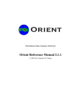
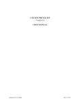
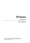
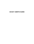
Figure 4.21 Modified Kamb contour plot of data shown in Figure 4.16 with contours at 10% density, and the Gradient option on. Figure 4.22 Modified Kamb contour plot of data shown in Figure 4.16 with contours at 10% density, and the Gradient and Fill contours options on. Figure 4.23 Lower hemisphere equal-area projection of poles to bedding (green) from Figure 4.13 with modified Kamb contours at 20% density, and minor fold axes (cyan). 30 Tutorial 5 – Contour Plots Open the file Vollmer 1981b from the Example Data folder (any of the .csv, .tsv. .ods, .xls, or .xlsx versions) in Orient, and click on the Spherical Projection icon. If not already done, remove the Schmidt net from the background. Click on the Preferences icon, and locate the Net pane under the Spherical Projection settings. Uncheck both Axes and Net. Next, in the Labels pane, change the Increment to -90, the Offset to 14, and the Size to 12. If still on from the previous tutorial, turn off eigenvector and confidence cone display in the Maxima panel. The Help Restore Defaults command can be used to reset all preferences if desired. In the Symbols pane two data types are available, F (minor fold axes) and S0 (bedding). Set the F Symbol Fill Color to cyan, and S0 Symbol Fill Color to light green. For S0, check both Contour and Gradient. Click on the gradient paint picker and select the YOR (Yellow Orange Red) preset. Finally, in the Contours pane set the Levels to 5. This gives modified Kamb contours at 20% density levels, and the plot should appear as in Figure 4.23 4.8 Coordinates and Rotations The rotations used for projection and data display are normally transparent to the user, and the default settings are sufficient in most cases. The default coordinates are local coordinates commonly used in geology (North at the top, and East at the right), however, it is easily configured for other common geographic or spherical coordinate systems, which is the first topic covered in in this section. The second topic covered here is coordinate system rotation, or projection rotation. In some cases it is useful or necessary to view data in a more specialized coordinate system, for example centered over a specific location, or chosen parallel to the data eigenvectors. The third topic is data rotation, which may be required for a number of reasons, such as paleomagnetic fold tests, or rotation of paleocurrent measurements back to horizontal. The primary coordinate system is selected in the Preferences dialog in the Spherical Projection Projection panel (Figure 4.24). In addition to the Projection and Hemisphere pulldown menus, there is an Orientation option where six geographic coordinate systems can be selected (Polar, Antipolar, Equatorial 0, Equatorial 90, Equatorial 180, and Equatorial 270) and six spherical systems (XY, ZX, YZ, YX, XZ, and ZY planes). Additionally, there are checkboxes for inverting the projection about the Y and X axes. These are used, for example, to produce plots like Figure 1.3, a plot of directed magnetic data displayed on both hemispheres. These options provide views along any of the three axes in either direction. The Axes display changes when these are modified, so the current coordinate system is clear, for example X Right, Y Top, Z Out is displayed for local coordinates. 31 Figure 4.24 Preferences dialog Spherical Projection Settings pane displaying the options for an equal-area upper hemisphere projection centered at latitude, longitude 0°, 0°. Note the Axes display, here X Out, Y Right, Z Top, gives the current position of the coordinate axes. Figures 4.25 to 4.30 are equal-area projections of 14,229 earthquake epicenters with magnitudes greater than 4.5 from 1980 to 1990 (data from NOAA) plotted on the six standard geographic coordinate systems. Figure 4.25 Upper hemisphere equal-area projection of 14,229 earthquake epicenters with magnitudes greater than 4.5 from 1980 to 1990, centered at latitude, longitude 0°, 0°, the Equatorial 0 coordinate system in Orient (data from NOAA). Figure 4.26 Equal-area projection of earthquake epicenters as in Figure 4.25 centered at 0°, 90°, the Equatorial 90 coordinate system in Orient. 32 Figure 4.27 Equal-area projection of earthquake epicenters as in Figure 4.25 centered at 0°, 180°, , the Equatorial 180 coordinate system in Orient. Figure 4.28 Equal-area projection of earthquake epicenters as in Figure 4.25 centered at 0°, -90° , the Equatorial 270 coordinate system in Orient. Figure 4.29 Equal-area projection of earthquake epicenters as in Figure 4.25 centered at 90°, 0°, the Polar coordinate system in Orient. Figure 4.30 Equal-area projection of earthquake epicenters as in Figure 4.25 centered at -90°, 0°, the Antipolar coordinate system in Orient. 33 The standard settings provide views of data along all coordinate axes, however it is also possible to select a view along an arbitrary axis using the Rotate Projection command. The Rotate Projection dialog is shown in Figure 4.31. Figure 4.31 The Rotate Projection dialog showing the settings for a rotation of 74.156° about the Z axis, which is currently at the top of the projection. For example, to produce a projection centered at latitude, longitude 41.764, -74.156, first set the coordinate system to Equatorial 0 (Figure 4.25). The projection is now centered at 0°, 0°, with X out, Y right, and Z top. Set Z as the Axis, enter 74.157 into the Angle edit box, and press Apply. The projection is now centered at 0°, -74.157°. Then set Y as the Axis, enter 41.764 into the Angle edit box, and press Apply. The projection is now centered at 41.764°, -74.157°. Figure 4.32 Equal-area projection of earthquake epicenters as in Figure 4.25 centered at latitude, longitude 41.764°, -74.157°. 34 In examining some data sets, such as crystallographic axes, it may be desirable to produce a plot whose axes are related to the distribution, such as the eigenvectors (Fisher et al., 1987). Figure 4.33 shows the Rotate Projection dialog with settings to rotate a data set to the maximum eigenvector. Figure 4.33 The Rotate Projection dialog showing the settings for a rotation to center the projection on the maximum eigenvector of the S0 data type. Figure 4.34 is a lower hemisphere equal-area modified Kamb contour plot of poles to bedding data shown in Figure 4.13, which is then shown rotated the maximum (Figure 4.35), intermediate (Figure 4.36), and minimum (Figure 4.37) eigenvectors. Figure 4.34 Lower hemisphere equal-area modified Kamb contour plot of poles to bedding from Figure 4.13 with contours at 20% density. Figure 4.35 Contour plot as in Figure 4.34, rotated to the maximum eigenvector of the data. 35 Figure 4.36 Contour plot as in Figure 4.34, rotated to the intermediate eigenvector of the data. Figure 4.37 Contour plot as in Figure 4.34, rotated to the minimum eigenvector of the data. The final topic in this section is data rotation. The principal is the same as projection rotation however the rotations are applied to the data. The data can be rotated about any of the coordinate axes, or about an arbitrary axis of any orientation (Figure 4.38). Figure 4.38 The Rotate Data dialog allows rotation of the data about any of the coordinate axes, or about an arbitrary axis of any orientation. Tutorial 6 – Geographic Coordinates Open the file Earthquakes with Continents from the Example Data folder (any of the .csv, .tsv. .ods, .xls, or .xlsx versions is fine) in Orient, and click on the Spherical Projection icon. The projection will be extremely cluttered. Open the Preferences dialog and select the Spherical Projections Symbols pane. For the data type CO, uncheck Symbol, check Polyline, and check Directed. For the data type EQ, set the Symbol Size to 1, the Stroke and Fill Colors to red, and the Stroke and Fill Opacities to 50%. Check Directed. Select the Net pane, uncheck Axes, and check Net. For the Y axis, uncheck both Major and Minor Great circles and Small circles. For the Z axis, check Major Great circles and Major Small circles, and set both Stroke Colors to a very light gray. 36 Select the Projection panel, set the Hemisphere to Upper Hemisphere, and the Orientation to Equatorial 0. The projection is now centered at latitude, longitude 0°, 0°, X is out, Y is right, Z is at the top, and the plot should appear as in Figure 4.25. To center the projection at latitude, longitude 41.764, -74.156, open the Rotate Projection dialog (Figure 4.31). Set Z as the Axis, enter 74.157 into the Angle edit box, and press Apply. The projection is now centered at 0°, -74.157°. Then set Y as the Axis, enter 41.764 into the Angle edit box, and press Apply. The projection is now centered at 41.764°, -74.157°. Tutorial 7 – Rotations Open the file Vollmer 1981 from the Example Data folder (any of the .csv, .tsv. .ods, .xls, or .xlsx versions is fine) in Orient, and click on the Spherical Projection icon. If not already done, remove the Schmidt net from the background. Click on the Preferences icon, and locate the Net pane under the Spherical Projection settings. Uncheck both Axes and Net. Next, in the Labels pane, change the Increment to -90, the Offset to 14, and the Size to 12. In the Spherical Projection settings, restore the projection to Lower hemisphere and Local coordinates. In the Symbols pane, uncheck Symbol for the S0 data type, and check both Contour and Gradient. Click on the gradient paint picker and select the BCYR (Blue Cyan Yellow Red) preset. Finally, in the Contours pane set Levels to 5. This gives modified Kamb contours at 20% density levels, and the plot should appear as in Figure 4.34. Use the Rotate Projection command to open the Rotate Projection dialog (Figure 4.33). Set Axis to Maxima, Data type to S0, and Eigenvector to Maximum to produce Figure 4.35, Intermediate for Figure 4.36, and Minimum for Figure 4.37. 4.9 Terminology of Spherical Projections The equal-area projection is correctly referred to as the Lambert azimuthal equal-area projection (Snyder, 1985), however in the context of orientation data analysis, as in structural geology, it is usually sufficiently clear to refer to it as the equal-area projection. The projected hemisphere should also be given in text and figure captions, as lower-hemisphere equal-area projection. Note that, although less commonly used, hyperboloidal equal-area and stereographic projections exist, and are used for some geologic data (Yamaji, 2008; Vollmer, 2011). The terminology can be confusing, but is important for scientific communication. The terms stereographic projection (Snyder, 1985) and stereonet (Bucher, 1944) in particular, are clearly defined but frequently misused. Early references (Schmidt, 1925; Billings 1942, 1954; Bucher, 1944; Sander, 1948, 1950, 1970; Phillips, 1954; De Sitter, 1956; Badgley, 1959; Turner and Weiss, 1963; Hills, 1963, Whitten, 1966; Ramsay, 1967, Hobbs et al., 1976) are careful to use correct terminology, as are most current structural geology texts (e.g., Marshak and Mitra, 1988; Van der Pluijm and Marshak, 2004; Pollard and Fletcher, 2005; Twiss and Moores, 2007; Ragan, 2009; Fossen, 2015). Note that: • • • • • • The equal-area projection is not a type of stereographic projection A stereonet, or Wulff net, is a stereographic net (Figure 4.7) A Schmidt net, or equal-area net (Figure 4.12), is not a stereonet Scatter plots and contour plots are not stereonets The phrase equal-area stereonet is a contradiction The phrase equal-area stereographic projection is a contradiction 37 Another term that is sometimes used in the context of spherical projections is stereogram, which is used generally to refer to a planar representation of a three-dimensional structure. Stereogram, however, is sometimes used more specifically to refer to a diagram produced by stereographic projection (Phillips, 1954). The phrase equal-area stereogram has been used to refer to a diagram produced by equal-area projection (Lisle and Leyshorn, 2004). However, if a stereogram is a diagram produced by a stereographic projection, then the phrase equal-area stereogram is a contradiction. The phrases equal-area projection (Snyder, 1985) and Schmidt net are clear and have a long history. It is common to see spherical projection scatter plots (Section 4.4) and contour plots (Section 4.7) labeled as stereonets. However, they are clearly not stereonets, so what they represent is unclear. The reader is required to guess, an unsatisfactory situation. The equal-area projection and the Schmidt net have a long and important history in structural geology, mislabeling them as stereonets does not give due credit. In 1925 Schmidt recognized that the stereographic projection was not suitable for orientation data analysis, and invented the Schmidt net, 90 years ago. 38 5. Kinematic Analysis Some data comprise planes that contain lines. These data may indicate movement along faults or shear directions, such as striae on slickenside surfaces. Other data, such as hinge lines in fold axial planes, or current directions in bedding planes, also have that characteristic, however this section deals only with the kinematic analysis of faults and shear zones. Numerous methods exist for the determination of stresses, strains, or displacements from populations of faults, Orient implements a kinematic analysis based on M-plane, or movement plane, geometry (Angelier, 1979; Marshak and Mitra, 1988; Twiss and Unruh, 1998; Marrett and Allmendinger, 1990; Twiss and Moores, 2007). Although the term fault is used here, the kinematic analysis can be applied to shear zones if the displacement directions can be determined. As the slip lineation lies within the fault plane, the displacement direction must lie in the plane containing the lineation and the pole to the fault, this plane is the M-plane. Figure 5.1 shows the geometric relationships with the M-plane shown in gray. Figure 5.1 Lower hemisphere equal-area projection of a normal fault, with a slip lineation (red), pole to the fault (blue) and the M-axis, or movement axis, (green), the M-plane is shown in gray. Directions P and T bisect the angle between the pole and slip line. Arrows are tangent lines that show the displacement sense of the hanging wall with respect to the footwall. Two additional kinematic axes can be defined within the M-plane, at ±45° from the lineation (Figure 5.1). These are commonly referred to to as the P-axis and T-axis, terms derived from first motion studies in seismology, however they should not be confused with stress axes. Rather P is an incremental shortening axis, and T is an extension axis. 39 Figure 5.3 A lower hemisphere equal-area slip tangent line diagram of the data shown in Figure 5.2. The arrows through the slip lineation projections show the displacement sense of the hanging wall with respect to the footwall (data from Angelier, 1979). Figure 5.2 A lower hemisphere equal-area sliplinear, or pole tangent line, diagram of a population of 38 Neogene normal faults from central Crete, Greece. The arrows through the fault pole projections show the displacement sense of the hanging wall with respect to the footwall (data from Angelier, 1979). The arrows drawn though the lineation and the fault normal are tangent lines, directed lines tangent to a projected point on a sphere. In Figure 5.1 tangent lines are drawn through the lineation and the fault pole projections to show the placement sense of the hanging wall with respect to the footwall. They can be viewed as instantaneous rotation vectors about the M-axis. The term slip-linear has been used for a tangent line drawn through the fault pole using this reference frame (Marshak and Mitra, 1988). Figure 5.2 shows a slip-linear diagram of a population of 38 Neogene normal faults from central Crete, Greece (data from Angelier, 1979). The term tangent-lineation has been used for the tangent line drawn through the fault pole showing the placement sense of the footwall with respect to the hanging wall (Twiss and Unruh, 1998; Twiss and Moores, 2007). However, the reference frame used in Figures 5.1 and 5.2 for slip-linears is compatible with the definition of fault slip as a displacement vector of the hanging wall with respect to the footwall, and has priority, so is the default setting. Since Orient offers both conventions, the term pole tangent line (tangent line through the projected fault pole) is used to include both slip-linear and tangent-lineation reference frames. A second type of tangent line can be drawn through the slip lineation within in the M-plane. This is referred to here as a slip tangent line (tangent line through the projected slip line), drawn though the projected lineation towards, or away from, the pole to the fault (Figure 5.1). This contains the same information as a pole tangent line. Note that many spherical projections of fault data in the literature show ticks or arrows parallel to the trend of the slip lineation, which is not the same. The P and T axes (Figure 5.1) indicate shortening and extension axes respectively, and fault kinematic analysis can therefore done by examining populations of P and T axes using moment tensors (Marrett and Allmendinger, 1990). When fault data is entered in Orient, normally a strike and dip for a fault 40 plane, and a trend and plunge for a slip lineation, Orient automatically generates M-planes, P-axes, and T-axes. An extension is added to the data type indicate each of the five data elements (Table 5.1). Data Type Extension Data Element .S Plane, fault, slickenside, or shear plane .L Line, slip direction, slickenline, or shear direction .M M movement plane .P P shortening axis .T T extension axis Table 5.1 Data type extensions automatically generated for kinematic data. Each of these extended data types can be plotted and analyzed independently. For kinematic analysis the P and T axes are contoured (Section 4.7), and their maximum values and scatter determined by eigenvector analysis (Section 4.5, Figures 5.3 and 5.4), and for the construction of beachball diagrams (Figure 5.5). Figure 5.3 Lower hemisphere equal-area projection of poles to M-planes (green), P shortening axes (red), and T extension axes (blue) for data in Figure 5.2. 41 Figure 5. 4 Lower hemisphere equal-area modified Kamb contour plot of the fault data from Figure 5.2 with 10% density contours on the P shortening axes. Figure 5.5 Projection as in Figure 5.3 with contours on the T extension axes. Figure 5.6 Lower hemisphere equal-area beachball diagram showing the P shortening and T extension quadrants using the data shown in Figure 5.3. Tutorial 8 – Kinematic Analysis Open the file Angelier 1979 from the Example Data folder (any of the .csv, .tsv. .ods, .xls, or .xlsx versions) in Orient, and click on the Stereographic Projection icon. If no settings have been previously 42 modified the projection will look as in Figure 5.7. The Help Restore Defaults command can be used to reset the preferences if desired. To remove the Schmidt net from the background, click on the Preferences icon, and locate the Net pane under the Spherical Projection Settings. Uncheck both Axes and Net. Next, in the Labels pane, change the Increment to -90, the Offset to 14, and the Size to 12. Next, go to the Symbols pane. Note that there are 5 data types displayed in the Data type pulldown list. Select SL.P, check Visible, then select SL.T and check Visible. At this point all data type elements should be displayed with a symbol as in Figure 5.8. The first step is to prepare a pole tangent line, or slip-linear, plot. In the Symbols pane uncheck Visible for all the elements except SL.S so only the poles to the fault planes are displayed. Now go to the Kinematics pane and check Tangent lines. The resulting plot is shown in Figure 5.2. Figure 5.7 Lower hemisphere equal-area scatter plot of fault data in Figure 5.2 showing fault normals (white), slip lines (red), and M-planes (green), with Schmidt net. Figure 5.8 Projection as in Figure 5.7 after turning off display of the Schmidt net, and showing the P shortening (magenta) and T extension (cyan) axes. Next prepare modified Kamb contour plots of the P shortening and T extension axes. Uncheck Tangent lines in the Kinematics pane, and open the Symbols pane. Uncheck Visible for SL.S. For SL.P, check the following: Visible, Symbol, Contour, and Gradient. Modify the defaults as follows. Set the Symbol Fill color to white, and the Symbol Size to 6. Click on the gradient color picker, and select YR (yellow red) from Preset. Next go to the Contours pane and set Levels to 5 to give modified Kamb contours at 20% density. The resulting plot is shown in Figures 5.9. 43 Figure 5.10 Projection as in Figure 5.10 with contours of the T extension axes. Figure 5.9 Lower hemisphere equal-area modified Kamb contour plot of the fault data from Figure 5.2 with 20% density contours of the P shortening axes. To prepare a contour plot for the T extension data, uncheck Visible for SL.P. For SL.T, check: Visible, Symbol, Contour, and Gradient. Set the symbol Fill color to white, and the Symbol Size to 6. Click on the gradient color picker, and select CB (cyan blue) from Preset. The resulting plot is shown in Figure 5.10. Finally, to prepare a beachball diagram, uncheck the SL.T options for Contour and Gradient, and set the Symbol Fill color to cyan. For SL.P, check Visible, uncheck Contour and Gradient, and set the Symbol Fill color to red. In the Kinematics pane check Beachball. The resulting plot is shown in Figure 5.6. 44 6. Orientation Plots 6.1 PGR Plot A triangular PGR (Point Girdle Random) eigenvalue plot is particularly useful when a summary diagram is required of numerous data sets. On the PGR plot a single point summarizes the type of orientation data distribution among point (or cluster), girdle, and random (or uniform) distributions. The PGR plot is also used in map domain analysis, where domains are defined in the Orientation Map portion of the program, by maximizing the total cylindricity index. Given the orientation matrix eigenvectors ε1, ε2, and ε3 for n data points, where the magnitudes ε1 ≥ ε2 ≥ ε3, the following are defined (Vollmer 1989): Point P = (ε1 - ε2)/n Girdle G = 2(ε2 - ε3)/n Random R = 3ε3/n Cylindricity C=P+G these have the property that: P+G+R=1 and form the basis of the triangular PGR plot. Cylindrical data sets plot near the top of the graph, along the P-G join, point distributions plot near the upper left (P), girdle distributions plot near the upper right (G), and random or uniformly distributed data will plot near the bottom of the graph (R). Figure 6.1 is a plot of bedding plane poles from a cylindrical fold in Ordovician graywackes (Vollmer, 1981), and Figure 6.2 is the corresponding PGR graph. These indicate a well defined girdle with a distinct maximum. Figure 6.1 Lower hemisphere equal-area modified Kamp contour plot of poles to bedding from a fold in Ordovician graywackes, Albany County, New York (data from Vollmer, 1981). Figure 6.2 PGR graph of data shown in Figure 6.1. 45 A contour plot of ice fabric c-axes (Kamb, 1959) is shown in Figure 6.3, which shows a much more scattered distribution, and plots nearer to the bottom of the PGR graph (Figure 6.4). Finally a plot of fold axes associated with the bedding data in Figure 5.1 is shown in Figure 6.5, and the associated PGR plot in Figure 6.6 showing a strong point cluster. Figure 6.4 PGR graph of data shown in Figure 6.3. Figure 6.3 Lower hemisphere equal-area modified Kamb contour plot of ice c-axes (data from Kamb, 1959). Figure 6.5 Lower hemisphere equal-area modified Kamb contour plot of minor fold axes associated with the bedding data in Figure 6.1. Figure 6.6 PGR plot of fold axis data in Figure 6.5 showing strong point cluster. 46 7. Orientation Maps Spherical projections aid in the analysis of the orientation data, such as rock foliations, but they do not display their spacial distribution. Understanding the spacial relationships of orientation data is often one of the primary goals of a geologist, particularly a structural geologist. A number of tools are provided in Orient to assist with spacial analysis. These include coordinate conversions, integration with mapping websites, and integration with Google Earth. Orient is designed to plot the spacial distributions of orientation data, and has the capability of calculating orientation data fields that can be used to study regional tends and to do structural domain analysis. For example, a common problem in mapping areas of complex geological structure is to identify domains of cylindrical folding. Orient provides unique capabilities to automatically search for such domains (Vollmer, 1990). 7.1 UTM, Latitude, Longitude, Conversion Orient includes UTM to latitude, longtitude and latitude, longtitude to UTM conversions (Snyder, 1987; Dutch 2015). Conversion among 14 datums, including WGS 1984 an, NAD 1983, is available. The Data UTM Conversion Dialog (Figure 7.1) can be accessed when there are either easting, northing coordinates, or latitude, longitude coordinates. Select the conversion, and the desired datum. The hemisphere can be specified using the UTM grid zone, or by hemisphere. Figure 7.1 UTM, latitude, longitude conversion dialog. Tutorial 9 – UTM Conversion Open the file World Earthquakes 1980-1990 Map from the included Example Data folder (any of the provided file formats is fine, .csv, .tsv, .ods, .xls, or .xlsx). Note that the file World Earthquakes 19801990 Sphere is formatted to plot the data on a spherical projection, and is not the one for this tutorial. This data is a set of 14,229 earthquake epicenters between 1980 and 1990 with magnitudes greater than 4.5 (data from NOAA). Next, open the UTM Conversion Dialog (Figure 7.1), select Latitude, longitude to UTM, WGS 1984, and UTM latitude zone. Press OK, and the conversion is done. Finally, select View Data Columns and check Zone, Easting, and Northing if not already checked. UTM grid zones and coordinates should all be displayed. If you want to get a taste of Tutorial 9, select one of the earthquake data rows, and select Data Show Location Google Maps Satellite. As this is a global data set, you may need to zoom out before determining where you are. 47 7.2 Google and Web Maps Integration A large number of internet web sites offer access to maps, including street maps, topographic maps, and terrain maps, by entering search terms or geographic coordinates. Google Maps is perhaps the most well known of these. Orient includes integration with a number of these sites, including Google Maps, ACME Mapper (which has many topographic maps), Bing Maps, Nokia HERE, OpenStreetMaps, and others. If a data file contains latitude and longitude coordinates, these can be opened directly from Orient. If the data contains UTM coordinates, they must first be converted to latitude, longitude as covered in Section 7.1. To see the location displayed in your default browser, select a data row containing latitude, longitude coordinates, and choose a website from the Data Show Location menu. 7.3 Google Earth Integration The program Google Earth is an invaluable tool in numerous areas, and has become a widely used tool in geologic mapping. Google provides an interface using KLM (Keyhole Markup Language) files that can contain geographic coordinates, viewing instructions, and many other details. Orient uses this interface to display outcrop locations, and symbols for orientation data measurements. Symbols are selected from the Preference Dialog Orientation Map Settings Symbols pane where various symbols can be selected, as well as color, size, and line width. The symbol size is set in meters in the KML length edit box, and the width in the KML width edit box. To save the file, use the File Export to Google Earth KML command. Double click the resulting file to open in Google earth. Tutorial 10 – Web and Google Earth Integration This tutorial covers internet web maps, such as Google Maps, as well as Google Earth integration. Open the file Sky Top from the included Example Data folder (any of the provided file formats is fine, .csv, .tsv, .ods, .xls, or .xlsx). This is a demonstration file with simulated geologic data for use in this tutorial. You may wish to use the View Data Columns command to close some of the unused columns. The file contains the latitude, longitude coordinates of one marker location, and eight simulated data points of four different types of geologic data, bedding, cleavage, joints, and slickenside lineations. For web map access, select one of the locations and choose a websites from the Data Show Location menu. The selected web map will display the location of the data point, you can then zoom in, or change display options as needed. In order to display orientation data symbols, as well as location, Orient writes KML files for Google Earth, so orientation symbols and complete data sets can be viewed. Open the Preference Dialog by clicking on its icon, select the Orientation Map Settings option, and the Symbols pane. Select the data types from the pulldown menu, and check just one symbol for each data type. For J, check Strike, select a strike line with two ticks, and set Stroke Color to light green. For L, check Line, select an arrow symbol, and set Stroke Color to magenta. For S0 check Strike, select a strike line symbol, and set Stroke Color to red. For S1, check Strike, select a strike line with a tooth, and set Stroke Color to red. Press OK when done. 48 Save the file as Sky Top.klm using the File Export to Google Earth KML command. Double click on it to open in Google Earth. The location (that I can see from the window in my university office) should come into view with the data symbols (Figure 7.2). For a quicker demonstration, there is a copy of the resulting file in the Example Data folder. Figure 7.2 Example data from the file Sky Top viewed in Google Earth. Example data types are S0 (bedding, red), S1 (cleavage, blue), J (joints, green), and a lineation (L, magenta). 7.4 Orientation Fields and Domain Analysis Spherical projections aid in the orientation analysis of data, but they do not show their spacial distribution. Therefore Orient provides tools for analyzing the spacial variation of orientation data, including orientation fields and structural domain analysis. Orientation fields are a way to look for regional patterns in data by defining eigenfoliations and eigenlineations on a grid over the area (Vollmer, 1990). One method is to define discrete subdomains that include all data within them, for example a one kilometer square area. A second method is to apply a weighting function to produce area-smoothed orientation values. For example, a common problem in mapping areas of complex geologic structure is to identify cylindrical domains within the map area (Ramsay, 1967). Figure 7.3 is an equal-area lower hemisphere 49 projection of poles to foliations from the Doverfjell mountains, Norway, and Figure 7.4 is a modified Kamb contour plot of the data. Their spacial distribution is shown in Figure 7.5, plotted using the Orientation Map command. Figure 7.3 Lower hemisphere equal-area projection of poles to 625 foliation planes from the Doverfjell Mountains, Norway (data from Vollmer, 1985). Figure 7.4 Modified Kamb contour plot of the data shown in Figure 7.3 with contours at 20% density. Figure 7.6 Subdomain orientation field of eigenfoliation strikes generated from the data shown in Figure 7.3. The strike tick marks represent the horizontal projection of the dip line. Figure 7.5 Orientation map of foliation strikes of the data shown in Figure 7.3. 50 Figure 7.7 Weighted orientation field of eigenfoliation dip lines generated from the data shown in Figure 7.3. The arrows represent the horizontal projections of the dip line. The geometry of the structure defined by the foliations is not obvious. Figure 7.6 is a subdomain orientation field defined on a one kilometer grid. Note that the number of data points within each subdomain varies, and that each has a discrete boundary. Figure 7.7 is a weighted orientation field where each grid node is generated as a weighted sum of all other data points. This map shows the horizontal projection of the dip lines, with steeper dips displayed as shorter lines. Structural domain analysis (Vollmer, 1990) is done by attempting to maximize a quantity, or index, related to the given problem. Orient provides several indexes that may be maximized, including point, girdle, and cylindricity indexes. To locate areas of cylindrical folding the cylindricity index is maximized: C = (ε1 + ε2 – 2ε3) / n Where ε is the orientation matrix eigenvalue for n data points, and ε1 ≥ ε2 ≥ 2ε3. For a set of domains the sum of the products of the domain indexes (C 1, C2, C3, ...) and the number of data points within each domain (n 1, n2, n3, ...): Z = C1n1 + C2n2 + C3n3 + ... is maximized. Because: n = n1 + n2 + n3 + ... the maximum possible value for Z is equal to n. The normalized sum is: C' = Z/n 51 The settings for the Orientation Map command are in the Preferences Dialog Orientation Map panels. For each data point, or field value, it is possible to plot a symbol in four directions, Line, Dip line, Strike, and Strike 180 (Figure 7.8). Figure 7.9 The Domain Search dialog box. Figure 7.8 Orient Preference dialog showing the Orientation Map Symbols pane. The options shown are to project strike lines as in Figure 7.6. Line is the direction of a line, or of the plane normal (θ). Dip line is the opposing direction (θ + 180°), and used to display a plane's dip direction. Strike is the plane strike (θ + 90°), and Strike is the opposing direction (θ – 90°). Only Line and Dip line can be projected. To display a projected strike symbol, select Dip line and the strike symbol shaped like a sideways T (Figures 7.6 and 7.8). The Length scale scales the length of the symbol. The KLM settings are for the display of data in Google Earth (Section 7.3). To conduct a domain search, define the extents of the map area in the Extents panel, select the Subdomain Method in the Field panel, along with the number of subdomains. Then use the Domain Search command, which displays the dialog shown in Figure 7.9. This is used to maximize the orientation index using an automated search process. The Value is the current value of the index, and N is the number of points used to calculate it. Domains are numbered from 1 to 9, zero represents an unassigned domain. Clear sets all subdomains to zero. Initialize sets all domains to the search domain. Search will attempt to grow the search domain. The search process iteratively checks to see if subtracting a subdomain from one domain and adding it to the search domain will increase the index. It can only do so if both domains remain connected. The user can manually edit domains, moving the mouse over the map will display subdomain information in the status bar, and clicking on a subdomain will add it to the search domain if possible. The constraint that the domains remain connected can cause edge effects, and vacant subdomains may also effect connectivity. The general procedure is to do a search on a desired number of domains, then manually edit them, and search again to see if a better solution is found. Once the search is completed, pressing OK will assign domains to each of the data points. The domains are added as attributes of the data, use the View Data Columns to view the Domain column. Extended data types are formed by appending domain extensions, D1 to D9, to the data type so each domain can be plotted independently, for example on a spherical projection. 52 Tutorial 11 – Domain Analysis Open the file Vollmer 1985 included Example Data folder (any of the provided file formats is fine, .csv, .tsv, .ods, .xls, or .xlsx). This is the data displayed in Figures 7.3 to 7.7, 625 foliation planes from the Doverfjell mountains, Norway. While folds are clearly present, the spherical projections (Figure 7.3 and 7.4) do not display a girdle pattern that would indicate cylindrical folding (there are spectacular sheath folds in the Doverfjell and adjacent Trollheimen ranges). The map of foliations (Figure 7.5) shows some areas of consistent orientation, but the location of cylindrical domains is not obvious. Click on the Orientation Map icon to display a map of the foliation data, then in the Orientation Map window, click on the Preferences icon. In the Orientation Map Extents pane, uncheck Auto scale, and enter the coordinates 890, 150 and 1010, 300 for the minimum and maximum map extents. To view the data, uncheck all symbols in the Maxima pane, and check only Strike in the Symbols pane. The result should appear as in Figure 7.5. To set up the domain search, uncheck Strike in the Symbols pane, and check Strike in the Maxima pane. In the Field pane the Method should be Subdomain, and Directed should be unchecked. Enter 12 and 15 for the number of subdomains. The coordinates are UTM based in meters, so this gives one square kilometer subdomains. The resulting map should be as in similar to Figure 7.6, except that the strikes are not projected. Press OK when done. To begin the domain search, select the Domain Search command form the Graph menu (Figure 7.9). Press Initialize to set all subdomains to 1, then press Search to grow domain 2. Change the search domain to 3, and press Search again. The result is should in Figure 7.10, which has a cylindricity index, c = 0.738. There are some edge effects, particularly where domain 1 wraps around the other two. Move the mouse over the map to see information about each subdomain. Clicking on one will change it to the current search domain, if all domains remain connected. Edit the domains by selecting a search domain and clicking on the map. When done, go back to the dialog and search on each domain again. If the domains are stable, they will not change. Figure 7.11 shows a stable solution with C = 0.851, an improvement over the previous value. Press OK when done. 53 Figure 7.10 Initial automatic domain search formed by grouping the subdomains of Figure 7.6 into three domains maximizing cylindricity. This configuration has a cylindricity index, C' = 0.738. Figure 7.11 Final domain configuration after iterative manual editing and automatic searching to find a stable configuration. This configuration has a cylindricity index, C' = 0.851. The map will now be cluttered with symbols, as the three new domains are plotted in addition to the field. Before cleaning up the map, open a spherical projection by clicking on the Spherical Projection icon in the data spreadsheet window, and then the Preferences dialog. In the Spherical Projection Net pane, uncheck Axes and Net, and in the Labels pane set Increment to -90, Offset to 14 and Size to 12, as in previous tutorials. In the Symbols pane, for data type S uncheck Visible. Then for data types S.D1, S.D2, and S.D3, the new data types, set the Symbol Fill Color to red, green, and blue respectively. In the Maxima pane, select only the Minimum eigenvector for S.D1, S.D2, and S.D3, and set the fill and stroke colors the same. The result should be as in Figure 7.12. Note that the three domains show well defined girdles. Turning off the data symbols give Figure 7.13, which suggests refolding of earlier folds about a northwest plunging axis. Next, open a PGR (Point Girdle Random) plot using the PGR Plot icon he data spreadsheet window. In the Preferences dialog PGR Plot Symbols pane set the Symbol Fill Color for S to white, and then for S.D1, S.D2, and S.D3, to red, green, and blue respectively, and increase the symbol sizes to 16. The resulting PGR plot (Figure 7.14) shows the relative changes in cylindricity from the whole area to the three domains. Note that domain 2 (green) has the strongest point distribution, and domain 3 (blue) has the strongest girdle distribution. 54 Figure 7.12 Lower hemisphere equal-area projection of data from Figure 7.3, with foliation poles color-coded by domain, and the great circle normal to the minimum eigenvector drawn for each domain. Figure 7.13 Synoptic plot of best fit girdles and axes of data shown in Figure 7.12. Figure 7.14 PGR graph of the three domains compared to the total data set (white). Figure 7.15 Data from Figure 7.5 color-coded by domain. To clean up the map, turn off the display of the maxima in the Orientation Map Maxima pane, turn off display of data type S symbols, and set Strike on with Stroke Color for S.D1, S.D2, and S.D3, to red, green, and blue respectively, giving the map in Figure 7.15. 55 As a final step, prepare lower hemisphere equal-area modified Kamb contour plots (Section 4.7) of the three domains (Figures 7.16, 7.17, and 7.18). Figure 7.16 Lower hemisphere equal-area midified Kamb contour plot of poles to foliation for domain 1 (red domain in Figures 7.10 to 7.15) contoured at 20% . Figure 7.17 Projection as in Figure 7.16 for domain 2 (green domain in Figures 7.10 to 7.15) Figure 7.18 Projection as in Figure 7.16 for domain 3 (blue domain in Figures 7.10 to 7.15) . 56 Acknowledgements Portions of this document were initially prepared for Teaching Structural Geology, Geophysics, and Tectonics in the 21st Century, On the Cutting Edge, held July 15-19, 2012 at the University of Tennessee, Knoxville, which rekindled my enthusiasm for completing this new version of Orient. I thank the conveners Barbara Tewksbury, Gregory Baker, William Dunne, Kip Hodges, Paul Karabinos, and Michael Wysession. I thank Eric Erslev, Steven Wojtal, Haakon Fossen, Josh Davis, Yvette Kueiper, Peter Hudleston, Robert Bauer, and Dazhi Jiang for discussions at various times on spherical projections. Emily Lubicich and Chistopher Gahn kindly helped with editing and pre-release testing. References Angelier, J., 1979. Determination of the mean principal directions of stresses for a given fault population. Tectonophysics, v. 56, p. T17-T26. Badgley, P.C., 1959. Structural methods for the exploration geologist. Harper and Brothers, New York, 280 pp. Barnes, J.W., 1995. Basic geologic mapping, 3rd Edition. Open University Press, Milton Keynes, UK. Billings, M.P., 1942. Structural geology. Prentice-Hall, New York, 473 pp. Billings, M.P., 1954. Structural geology, 2nd edition. Prentice-Hall, New York, 514 pp. Bingham, C., 1974. An antipodally symmetric distribution on the sphere. Ann. Stats., v. 2, p. 12011225. Bucher, W.H., 1944. The stereographic projection, a handy tool for the practical geologist. Journal of Geology, v. 52, n.3, p. 191-212. Cheeney, R.F., 1983. Statistical methods in geology. George Allen & Unwin, London. 169 p. Davis, J.C., 1986, Statistics and data analysis in geology. Wiley, 646 pp. De Sitter, L.U, 1956. Structural Geology. McGraw-Hill Book Company, Inc., London, New York, Toronto. 552 p. Dutch, S., 2015. Converting UTM to latitude and longitude (or vice versa). www.uwgb.edu/dutchs/usefuldata/utmformulas.htm (accessed 27 April 2015). Cheeney, R.F., 1983. Statistical methods in geology. Allen & Unwin, 169 pp. Diggle, P.J., and Fisher, N.I., 1985, Sphere: a contouring program for spherical data. Computers & Geoscience, v. 11, p. 725-766. Fisher, N.I., Lewis, T., and Embleton, B.J., 1987. Statistical analysis of spherical data. Cambridge University Press, Cambridge, 329 pp. Fosson, H., 2015. Structural geology, 2nd Edition. Cambridge University Press, Cambridge, 463 pp. Hills, E.S., 1963. Elements of structural geology. Chapman & Hall, London, 483 p. Hobbs, B.E., Means, W.D., and Williams, P.F., 1976. An outline of structural geology. Wiley, New York, 571 pp. Howarth, R.J., 1999. Measurement, portrayal and analysis of orientation data and the origins of early modern structural geology (1670-1967). Proceedings of the Geologists' Association, v. 110, p. 273309. Kamb, W.B., 1959. Ice petrofabric observations from Blue Glacier, Washington, in relation to theory and experiment. Journal Geophysical Research, v. 64, p. 1891-1909. Knopf, E.B., and Ingerson, E., 1938. Structural petrology. Geological Socity of America Memoir 6, 270 pp. 57 Lisle, R.J. and Leyshorn, P.R., 2004. Stereographic projection techniques for geologists and civil engineers, 2nd edition. Cambridge University Press, Cambridge, 112 pp. Mardia, K.V., 1972. Statistics of Directional Data. Academic Press. Mardia, K.V., and Jupp, P.E., 2000. Directional statistics. John Wiley & Sons, Ltd., Chichester, UK. 430 p. Mardia, K.V., and Zemroch, P.J., 1977. Table of maximum likelihood estimates for the Bingham distribution. Journal of Statistical Computation and Simulation, v. 6, p. 29-34. Marrett, R., and Allmendinger, R.W., 1990. Kinematic analysis of fault-slip data. Journal of Structural Geology, v. 12, p. 973-986. Marshak, S., and Mitra, G., 1988. Basic methods of structural geology. Prentice Hall, 446 p. Parker, J.M., 1942. Regional systematic jointing in slightly deformed sedimentary rocks. Geological Society of America Bulletin, v. 53, p. 381-408. Phillips, F.C., 1954. The use of stereographic projection in structural geology. Edward Arnold, London, 86 pp. Pollard, D.D. and Fletcher, R.C., 2005. Fundamentals of structural geology. Cambridge University Press, Cambridge, 463 500 pp. Ragan, 2009. Structural geology: an introduction to geometrical techniques, 4th edition. Cambridge University Press, Cambridge. 602 pp. Ramsay, J.G., and Huber, M.I., 1987. The techniques of modern structural geology, volume 2: folds and fractures. Academic Press, 700 pp. Sander, B., 1970. An introduction to the study of fabrics of geological bodies, 1st English edition. Pergamon Press, Oxford. 641 p. [Translated from Sander, 1948, 1950. German edition. SpringerVerlag]. Schmidt W., 1925. Gefügestatistik. Tschermaks Mineralogische und Petrographische Mitteilungen 38, p. 392–423. Snyder, J. P., 1987. Map projections: a working manual. United States Geological Survey Professional Paper 1395, 383 p. Turner, F.J. and Weiss, L.E., 1963. Structural analysis of metamorphic tectonites. McGraw-Hill Book Company, New York, 545 pp. Twiss, R.J., 1990. Curved slickenfibers; a new brittle shear sense indicator with application to a sheared serpentinite. Journal of Structural Geology, v. 11, p. 471-481. Twiss, R.J., and Unruh, J.R., 1998. Analysis of fault slip inversions: do they constrain stress or strain rate? Journal of Geophysical Research,. v. 103, p. 12205-12222. Twiss, R.J. and Moores, 2007. Structural geology, 2nd edition. W.H. Freeman, New York, 736 pp. Van der Pluijm, B.A. and Marshak, S., 2004. Earth structure, 2nd edition. W.W. Norton, New York, 656 p. Vollmer, F.W., 1981. Structural studies of the Ordovician flysch and melange in Albany County, New York: M.S. Thesis, State University of New York at Albany, Advisor W.D. Means, 151 p. Vollmer, F.W., 1985. A structural study of the Grovudal fold-nappe, western Norway. Ph.D. Thesis, University of Minnesota, Minneapolis, Advisor P.J. Hudleston, 233 p. Vollmer, F.W., 1988. A computer model of sheath-nappes formed during crustal shear in the Western Gneiss Region, central Norwegian Caledonides. Journal of Structural Geology, v. 10, p. 735-743. Vollmer, F.W., 1989. A triangular fabric plot with applications for structural analysis (abstract). Eos, v. 70, p. 463. Vollmer, F.W., 1990. An application of eigenvalue methods to structural domain analysis. Geological Society of America Bulletin, v. 102, p. 786-791. 58 Vollmer, F.W., 1993. A modified Kamb method for contouring spherical orientation data. Geological Society of America Abstracts with Programs, v. 25, p. 170. Vollmer, F.W., 1995. C program for automatic contouring of spherical orientation data using a modified Kamb method: Computers & Geosciences, v. 21, p. 31-49. Vollmer, F.W., 2015. Orient 3: Spherical projection and orientation data analysis program. www.frederickvollmer.com. Vollmer, F.W., 2011. Automatic contouring of two-dimensional finite strain data on the unit hyperboloid and the use of hyperboloidal stereographic, equal-area and other projections for strain analysis. Geological Society of America Abstracts with Programs, v. 43, n. 5, p. 605. Vollmer, F.W., 2015. Orient 3 User Manual www.frederickvollmer.com. [this document] Whitten, E.H.T., 1966. Structural geology of folded rocks. Rand McNally, Chicago, 663 pp. Yamaji, A., 2008. Theories of strain analysis from shape fabrics: A perspective using hyperbolic geometry. Journal of Structural Geology, v. 30, p. 1451-1465. 59 History 3.0.1.0 (2015-05-30) • Fixed bug importing dip direction (reported by Ben Michael Frieman). 3.0.0.77 (2015-05-01) • First release of Orient 3. Complete rewrite with numerous fixes and upgrades, over 500,000 lines of code, tested in 77 pre-release versions. Compiled, tested, and debugged on Macintosh OS X, Windows, and Linux. 2.1.2 (2012-10-31) • Last release of Orient 2. 1.0.0 (1986) • First release of Orient 1. Introduced modified Kamb contouring, PGR plots, and automated domain analysis (see Vollmer, 1988 and 1990 for example plots created in Orient 1). 60