1
A Tutorial for Preparing GEOtop Input Files with
JGrass
Erica Ghesla & Riccardo Rigon
Trento, April 2006
ISBN 10: 88-8443-153-0
ISBN 13: 978-88-8443-153-0
Translation by Joseph E. Tomasi
Readme
This ebook was written by Erica Ghesla and Riccardo Rigon (University of Trento, Department
of Civil and Environmental Engineering).
It is distributed according to the CREATIVE COMMONS deed: Attribution-NoDerivs 2.5
According to this license type you are free to:
• copy, distribute, display, and perform the work
• to make commercial use of the work
Under the following conditions:
• Attribution. You must attribute the work in the manner speciied by the author or licensor.
• No Derivative Works. You may not alter, transform, or build upon this work.
• For any reuse or distribution, you must make clear to others the license terms of this work.
Any of these conditions can be waived if you get permission from the copyright holder.
Your fair use and other rights are in no way affected by the above. This is a human-readable
summary of the Legal Code (the full license) that can be consulted at:
http://creativecommons.org/licenses/by-nd/2.5/legalcode
4
Contents
1 Introduction
1
1.1
JGrass . . . . . . . . . . . . . . . . . . . . . . . . . . . . . . . . . . . . . . . . . . . .
1
1.2
GEOtop . . . . . . . . . . . . . . . . . . . . . . . . . . . . . . . . . . . . . . . . . . .
1
2 Preliminary Operations
3
2.1
Installation of JGrass
. . . . . . . . . . . . . . . . . . . . . . . . . . . . . . . . . . .
3
2.2
Creating of a New Location . . . . . . . . . . . . . . . . . . . . . . . . . . . . . . . .
3
2.3
Importing the DEM (Digital Elevation Model )
. . . . . . . . . . . . . . . . . . . . .
5
2.3.1
Example . . . . . . . . . . . . . . . . . . . . . . . . . . . . . . . . . . . . . . .
6
2.3.2
Execution from the Command Line . . . . . . . . . . . . . . . . . . . . . . . .
7
Setting Up the Active Working Region . . . . . . . . . . . . . . . . . . . . . . . . . .
8
2.4.1
9
2.4
2.5
Example . . . . . . . . . . . . . . . . . . . . . . . . . . . . . . . . . . . . . . .
Viewing the Imported Map . . . . . . . . . . . . . . . . . . . . . . . . . . . . . . . . 11
3 Data Preprocessing for the Extraction of the Hydrographic Basin
3.1
Pitfiller . . . . . . . . . . . . . . . . . . . . . . . . . . . . . . . . . . . . . . . . . . . 13
3.1.1
3.2
Example . . . . . . . . . . . . . . . . . . . . . . . . . . . . . . . . . . . . . . . 19
MarkOutlets . . . . . . . . . . . . . . . . . . . . . . . . . . . . . . . . . . . . . . . . 22
3.4.1
3.5
Example . . . . . . . . . . . . . . . . . . . . . . . . . . . . . . . . . . . . . . . 17
DrainDir . . . . . . . . . . . . . . . . . . . . . . . . . . . . . . . . . . . . . . . . . . . 18
3.3.1
3.4
Example . . . . . . . . . . . . . . . . . . . . . . . . . . . . . . . . . . . . . . . 14
FlowDirections . . . . . . . . . . . . . . . . . . . . . . . . . . . . . . . . . . . . . . . 16
3.2.1
3.3
13
Example . . . . . . . . . . . . . . . . . . . . . . . . . . . . . . . . . . . . . . . 22
ExtractNectwork . . . . . . . . . . . . . . . . . . . . . . . . . . . . . . . . . . . . . . 24
3.5.1
Determination of the Network Using the Contributing Areas (or the Magnitude) 25
3.5.2
Determination of the Network Using the Contributing Areas and the Slopes . 27
3.5.3
Determination of the Network Using the Curvatures . . . . . . . . . . . . . . 31
i
CONTENTS
4 Extraction of the Basin of Interest
4.1
39
WaterOutlets . . . . . . . . . . . . . . . . . . . . . . . . . . . . . . . . . . . . . . . . 39
5 Input Maps for GEOtop
43
5.1
Format of the Input Files . . . . . . . . . . . . . . . . . . . . . . . . . . . . . . . . . 43
5.2
Creation of the Input Maps for GEOtop . . . . . . . . . . . . . . . . . . . . . . . . . 44
5.2.1
Slope
. . . . . . . . . . . . . . . . . . . . . . . . . . . . . . . . . . . . . . . . 48
5.2.2
Nabla (Laplacian) . . . . . . . . . . . . . . . . . . . . . . . . . . . . . . . . . 51
5.2.3
Aspect . . . . . . . . . . . . . . . . . . . . . . . . . . . . . . . . . . . . . . . . 53
5.2.4
Dist2Outlets . . . . . . . . . . . . . . . . . . . . . . . . . . . . . . . . . . . . 55
5.2.5
Channel Network . . . . . . . . . . . . . . . . . . . . . . . . . . . . . . . . . . 57
ii
List of Figures
2.1
Accessing a mapset from the main menu. . . . . . . . . . . . . . . . . . . . . . . . .
4
2.2
Accessing a mapset from the toolbar. . . . . . . . . . . . . . . . . . . . . . . . . . . .
4
2.3
The dialog box for the selection of the workspace from a list of available ones. . . . .
4
2.4
Importing digital data into JGrass. . . . . . . . . . . . . . . . . . . . . . . . . . . . .
5
2.5
The icon to click in order to import digital data into JGrass. . . . . . . . . . . . . .
5
2.6
Importing digital data into JGrass. . . . . . . . . . . . . . . . . . . . . . . . . . . . .
6
2.7
r.in.ascii. Dialog box for the selection of the file to import to JGrass. . . . . . . . . .
6
2.8
The icon to click in order to view the console. . . . . . . . . . . . . . . . . . . . . . .
7
2.9
The JGrass Console. . . . . . . . . . . . . . . . . . . . . . . . . . . . . . . . . . . . .
7
2.10 Execution of the r.in.ascii command from the command line. . . . . . . . . . . . . .
7
2.11 The g.region icon . . . . . . . . . . . . . . . . . . . . . . . . . . . . . . . . . . . . . .
9
2.12 The g.region dialog box . . . . . . . . . . . . . . . . . . . . . . . . . . . . . . . . . . . 10
2.13 Displaying a map in JGrass. . . . . . . . . . . . . . . . . . . . . . . . . . . . . . . . . 11
2.14 Selecting the toolbar with the d.rast command icon. . . . . . . . . . . . . . . . . . . . 11
2.15 Displaying a map in JGrass. . . . . . . . . . . . . . . . . . . . . . . . . . . . . . . . . 12
2.16 The result of the importation process. DEM of the Flanginec Basin. . . . . . . . . . 12
3.1
Executing the h.pitfiller command. . . . . . . . . . . . . . . . . . . . . . . . . . . . . 13
3.2
Executing the h.pitfiller command. . . . . . . . . . . . . . . . . . . . . . . . . . . . . 14
3.3
The h.pitfiller icon. . . . . . . . . . . . . . . . . . . . . . . . . . . . . . . . . . . . . . 14
3.4
h.pitfiller. Dialog box where the names of the input and output maps are specified. . . 15
3.5
h.pitfiller. Depitted elevation map. The Flanginec Basin. . . . . . . . . . . . . . . . . 15
3.6
The h.flowdirections icon. . . . . . . . . . . . . . . . . . . . . . . . . . . . . . . . . . 16
3.7
h.flowdirections. Dialog box where the names of the input and output maps are specified. 17
3.8
h.flowdirections. Drainage directions map. The Flanginec Basin. . . . . . . . . . . . 17
3.9
The h.draindir icon. . . . . . . . . . . . . . . . . . . . . . . . . . . . . . . . . . . . . 18
3.10 h.draindir. Dialog box where the names of the input and output maps are specified. . 19
3.11 h.draindir. Map of the corrected drainage directions. The Flanginec Basin.
iii
. . . . . 20
LIST OF FIGURES
3.12 h.draindir. Total contributing areas map based on the corrected drainage directions.
The unit of measurement is pixels. The Flanginec Basin.
. . . . . . . . . . . . . . . 21
3.13 The h.markoutlets icon. . . . . . . . . . . . . . . . . . . . . . . . . . . . . . . . . . . 22
3.14 h.markoutlets. Dialog box where the names of the input and output maps are specified. 23
3.15 h.markoutlets. Corrected drainage directions map with the region outlets marked.
The Flanginec Basin. . . . . . . . . . . . . . . . . . . . . . . . . . . . . . . . . . . . . 23
3.16 The h.extractnetwork icon. . . . . . . . . . . . . . . . . . . . . . . . . . . . . . . . . 24
3.17 h.extractnetwork. Dialog box where the names of the input and output maps are
specified. . . . . . . . . . . . . . . . . . . . . . . . . . . . . . . . . . . . . . . . . . . . 25
3.18 h.extractnetwork. Map of the hydrographic network obtained by imposing a threshold
on the contributing areas. The network points are marked in red (assigned value of
2). The map represents an area of the Province of Trento. . . . . . . . . . . . . . . . 26
3.19 The h.gradient icon. . . . . . . . . . . . . . . . . . . . . . . . . . . . . . . . . . . . . 27
3.20 h.gradient. Dialog box where the names of the input and output maps are specified. . 28
3.21 h.gradient. Gradient map. The Flanginec Basin. . . . . . . . . . . . . . . . . . . . . 28
3.22 h.extractnetwork. Dialog box where the names of the input and output maps are
specified. . . . . . . . . . . . . . . . . . . . . . . . . . . . . . . . . . . . . . . . . . . . 29
3.23 h.extractnetwork. Map of the hydrographic network obtained by imposing a threshold
on the product of the contributing areas and the gradient. The Flanginec Basin. . . . 30
3.24 The h.curvatures icon. . . . . . . . . . . . . . . . . . . . . . . . . . . . . . . . . . . . 31
3.25 h.curvatures. Dialog box where the names of the input and output maps are specified. 32
3.26 h.curvatures. Map of the tangent curvature (left), profile curvature (right), and
planar curvature (bottom) of the Flanginec Basin. . . . . . . . . . . . . . . . . . . . . 32
3.27 Subdivision of the pixels by curvature. . . . . . . . . . . . . . . . . . . . . . . . . . . 34
3.28 The h.tc icon. . . . . . . . . . . . . . . . . . . . . . . . . . . . . . . . . . . . . . . . . 34
3.29 h.tc. Dialog box where the names of the input and output maps are specified. . . . . . 35
3.30 h.tc. Map of the topological classes, with classification according to 9 categories. . . . 36
3.31 h.tc. Map of the topological classes, reclassified according to 3 categories. The concave sites are marked in yellow, the convex sites are marked in red, and the planar
ones are in blue. . . . . . . . . . . . . . . . . . . . . . . . . . . . . . . . . . . . . . . 36
3.32 h.extractnetwork. Dialog box where the names of the input and output maps are
specified. . . . . . . . . . . . . . . . . . . . . . . . . . . . . . . . . . . . . . . . . . . . 37
3.33 h.extractnetwork. Map of the hydrographic network obtained by imposing a threshold
value on the contributing areas. The Flanginec Basin. . . . . . . . . . . . . . . . . . 38
iv
LIST OF FIGURES
4.1
The h.wateroutlet icon. . . . . . . . . . . . . . . . . . . . . . . . . . . . . . . . . . . 39
4.2
h.wateroutlet. Dialog box requiring the names of the input maps and the closing
section coordinates. The blue circle marks the area where the closing section was
chosen. The red circle shows the value of the network map in correspondence of
the selected point (the value is 2 therefore the point is effectively part of the channel
network). . . . . . . . . . . . . . . . . . . . . . . . . . . . . . . . . . . . . . . . . . . 40
4.3
h.wateroutlet. Mask of the extracted subbasin superimposed onto the channel network
map. The Flanginec Basin. . . . . . . . . . . . . . . . . . . . . . . . . . . . . . . . . 41
4.4
h.wateroutlet. Map of the extracted subbasin. The Flanginec Basin. . . . . . . . . . . 41
5.1
r.mapclac. Command window where the expression to be calculated is input. . . . . . 45
5.2
h.draindir. Map of the corrected drainage directions of the extracted basin. The
Flanginec Basin. . . . . . . . . . . . . . . . . . . . . . . . . . . . . . . . . . . . . . . 46
5.3
h.draindir. Total contributing areas map of the extracted basin. The Flanginec Basin. 46
5.4
h.extractnetwork. Map of the channel network. The Flanginec Basin. . . . . . . . . . 47
5.5
h.gradient. Map of the gradient of the extracted basin. The Flanginec Basin. . . . . . 47
5.6
The h.slope icon. . . . . . . . . . . . . . . . . . . . . . . . . . . . . . . . . . . . . . . 48
5.7
h.slope. Dialog box where the names of the input and output maps are specified. . . . 49
5.8
h.slope. Choosing the output map format. The Flanginec Basin. . . . . . . . . . . . . 49
5.9
h.slope. Choosing the output map format. The Flanginec Basin. . . . . . . . . . . . . 49
5.10 h.slope. Naming the output map to be generated. The Flanginec Basin. . . . . . . . . 50
5.11 h.slope. Map of the slopes calculated along the drainage directions. The Flanginec
Basin. . . . . . . . . . . . . . . . . . . . . . . . . . . . . . . . . . . . . . . . . . . . . 50
5.12 The h.nabla icon. . . . . . . . . . . . . . . . . . . . . . . . . . . . . . . . . . . . . . . 51
5.13 h.nabla. Dialog box where the names of the input and output maps are specified. . . . 52
5.14 h.nabla. Map of the Laplacian, distinguishing between concave, convex, and planar
sites. The Flanginec Basin. . . . . . . . . . . . . . . . . . . . . . . . . . . . . . . . . 52
5.15 The h.aspect icon. . . . . . . . . . . . . . . . . . . . . . . . . . . . . . . . . . . . . . 53
5.16 h.aspect. Dialog box where the names of the input and output maps are specified. . . 54
5.17 h.aspect. The aspect map. The Flanginec Basin. . . . . . . . . . . . . . . . . . . . . 54
5.18 The h.D2O icon. . . . . . . . . . . . . . . . . . . . . . . . . . . . . . . . . . . . . . . 55
5.19 h.D2O. Dialog box where the names of the input and output maps are specified. . . . 56
5.20 h.D2O. Map of the distance of each point from the basin outlet. The Flanginec Basin. 56
5.21 The r.mapcalc icon. . . . . . . . . . . . . . . . . . . . . . . . . . . . . . . . . . . . . 57
5.22 The r.mapcalc graphic interface. . . . . . . . . . . . . . . . . . . . . . . . . . . . . . 58
v
LIST OF FIGURES
5.23 Map of the drainage directions with 10 assigned in correspondence of the channel
network. The Flanginec Basin. . . . . . . . . . . . . . . . . . . . . . . . . . . . . . . 59
vi
1
Introduction
1.1
JGrass
JGrass is a GIS based mainly on the analysis of raster and contains innovated algorithms for
the analysis of landscape shapes necessary in order to delineate the hydrogeological risk zones. In
JGrass have been moreover implemented hillslope stability models of stability and floods generation
models.
1.2
GEOtop
GEOtop [5, 11, 9], came to be through the will of Riccardo Rigon and in order to answer to a
series of converging topics: the desire to model evapotranspiration and eco-hydrological phenomena,
slope stability [7] and slope hydrology in general [12], as well as snow cover evolution [6, 8].
GEOtop is a terrain-based model, it is in fact based on the use of digital terrain models and
exploits the knowledge of the interactions between river basin morphology and basin processes. It
is a distributed model, all the simulated variables are returned for every pixel of the basin. It is a
hydrological model, it simulates all the components of the hydrological cycle, not only the water
budget but also the energy budget, the two budget equations are coupled by the evapotranspiration
and soil temperature terms, the soil temperature term also controls the hydraulic conductivity of the
soil and snow cover accumulation [6]). The model has been applied in the study of the hydrological
cycle of the Serraia Lake (Trento) [14] and to the data of the SGP97 experiment [5], the model was
validated with these data. A complete description of the model is found in [5] and [13], while [4]
contains an analysis of the effects of topography in the redistribution of hydrological flows.
For further information please refer to the literature listed in the bibliography and, if necessary,
to Rigon’s presentation [2004] [10].
The present tutorial has been written to facilitate the procedures of preparation of the geographic spatial inputs for the hydrological model GEOtop. Through the use of the GIS JGrass it
is possible to run easely advance analyses for the creation of maps which: water-drainage directions, total contributing areas, channel network, map of the convexities, slopes, aspect and others
important geomorfological parameters. These quantities are necessary inputs for the simulation of
the hydrological cycle by mass and energy budgets.
1. Introduction
2
2
Preliminary Operations
2.1
Installation of JGrass
The JGrass installation package can be found at the www.hydrologis.com web site, in the JGrass
section. For information about installation please refer to the aforementioned web site, the JGrass
User Manual [1], and the JGrass Wiki site. For particular problems you can consult the mailing
list, the address is available at the www.hydrologis.com web site.
The first steps to take include:
• understanding the JGrass interface;
• understanding what a location is;
• understanding what a digital terrain model (DTM) is ;
• understanding what is the active working region and how to set it up.
All these concepts are explained in detail in the JGrass User Manual [1], there follows here only a
brief summary.
2.2
Creating of a New Location
Once the program has been installed, it is necessary to create a workspace, also called location.
The location will contain information relative to the region and the processed maps will be saved
therein. For instructions on how to create a new location please refer to the JGrass User Manual
[1].
Once the location has been created it is possible to access the new workspace, from the main menu
select:
File ⇒ Load Workspace
or else click directly on the icon as shown in figure 2.2.
In both cases a dialog box will appear from which to select a working mapset. Click on the name of
the desired working location (in the example shown the location is flan geotop) and then click the
Finish button. An example of this operation is shown in figure 2.3. The workspace will appear, as
partially shown in figure 2.4.
2. Preliminary Operations
Figure 2.1: Accessing a mapset from the main menu.
Figure 2.2: Accessing a mapset from the toolbar.
Figure 2.3: The dialog box for the selection of the workspace from a list of available ones.
4
2. Preliminary Operations
2.3
Importing the DEM (Digital Elevation Model )
The first necessary operation is to import the digital terrain data of the area that you wish
to analyze into JGrass. The imported DEM is the basis from which the maps necessary for the
execution of GEOtop are generated.
The command to execute is r.in.ascii, from the main menu select:
Gis ⇒ Import/Export Tool s
as shown in figure 2.4.
Figure 2.4: Importing digital data into JGrass.
In so doing a new toolbar appears, shown in figure 2.5. To view the importation command dialog
box, click on the icon as shown in figure 2.5.
Figure 2.5: The icon to click in order to import digital data into JGrass.
The command can also be executed by selecting:
Gis ⇒ Import/Export Tools ⇒ r.in.ascii
as shown in figure 2.6.
5
2. Preliminary Operations
Figure 2.6: Importing digital data into JGrass.
2.3.1
Example
Let us import the DEM of interest, it is the starting point for the generation of the input files
necessary for the execution of the GEOtop program. Figure 2.7 shows the dialog box where the
file to be imported is selected. Click on the Browse button to select the file to be imported. The
program requires you to specify the value that has been assigned to the null value points of the
map to be imported, in the example it is -9999 (when the value of a point of the map is unknown,
these are assigned either a number or a symbol so that they can be recognised. In many cases the
asterisk, *, is used or another symbol. In these cases JGrass requires you to specify the null value so
that it can distinguish it from points of known value). Specify a name to give to the imported map
within JGrass. Click ok in order to execute the command. In this way the map will be imported.
Figure 2.7: r.in.ascii. Dialog box for the selection of the file to import to JGrass.
6
2. Preliminary Operations
2.3.2
Execution from the Command Line
The JGrass commands can be executed directly from the command line without viewing the
dialog box. To view the console click the icon as shown in figure 2.8.
Figure 2.8: The icon to click in order to view the console.
Figure 2.9: The JGrass Console.
To execute programs from the ”command line” you need to know the syntax to use. If you are
unsure of the exact syntax it is sufficient to type ”command name –usage” and then hit enter, the
string to use will appear on the console. The execution of r.in.ascii from the comand line is shown
in figure 2.10:
Figure 2.10: Execution of the r.in.ascii command from the command line.
7
2. Preliminary Operations
• [–quiet] : allows you to follow the evolution of the command;
• [–verbose] : shows the entire evolution of the command and the internal console messages,
this option can also be activated with the information icon of the console;
• [–usage] : allows you to view the syntax that is to be used in order to execute a command
(you must write: r.in.ascii –usage), this string must not be included for the execution of the
command;
• –ascii <ascii>: the map to be imported, the string <ascii> is to be replaced with the name
of the map to be imported;
• –map@mapset <map@mapset>: name to be assigned to the new map and the mapset where
it will be saved, the string <map@mapset> is to be replaced with the name of the map (map)
and the mapset (@mapset) where it is to be saved;
• [–novalue <novalue>] : value to be assigned to the ”null value” points, this term is not strictly
necessary, if it is not specified the program will automatically assign the value of -9999.0;
• [–usegui] : allows you to view the dialog box of the command (you must write r.in.ascii
–usegui ), this string must not be included for the execution of the command;
to execute r.in.ascii, as in the example in paragraph 2.3.1, it is sufficient to write:
r.in.ascii –ascii /Users/erica/Desktop/eclipse/workspace/jgrass1/DTM –map@mapset DTM@flan
geotop
For further information on the use of the console please refer to the JGrass User Manual, [1].
2.4
Setting Up the Active Working Region
Before viewing the imported map it is necessary to set up the active working region. This
procedure allows you to assign the coordinates and resolution of the imported map to the display
screen. The command to execute is g.region, from the main menu select:
Gis ⇒ Region Tools ⇒ Region Manager
as shown in figure 2.11. A dialog box will appear where the information about to the region is
input, an example is shown in figure 2.12.
8
2. Preliminary Operations
Figure 2.11: The g.region icon
The g.region command can be executed from the console command line:
g.region [–quiet] [–verbose] [–version] [–usage] –west <west> –east <east> –north <north> –south
<south> –map <map> –resolution <resolution> [–default] [–usetoolbar] [–usegui]
2.4.1
Example
To set up the working region, click the icon, as explained in paragraph 2.11. The name of the
map of interest can be input directly into the specific text box, which is found in correspondence of
the string ”map selection”, or else by clicking the Browse button and then selecting from the list
of available maps. Once a map has been selected click the ”set region from map” button in order
to set up the region. The information relative to the region will then appear, as shown in figure
2.12.
It is important that a lot of attention be given to this operation as all the calculations that will be
carried out afterwards depend on a correct setup of the working region. It is necessary to verify
that the numbers which indicate the resolution (found in the text boxes beside the strings nsres,
pixel dimension in a north-south direction, and ewres, pixel dimension in an east-west direction)
be integers. If necessary, modify the coordinates of the region boundary so as to obtain whole
number values for the resolution (the coordinates can be modified so that the difference between
the North-South and the East-West coordinates be multiples of the pixel resolution).
9
2. Preliminary Operations
Figure 2.12: The g.region dialog box
10
2. Preliminary Operations
2.5
Viewing the Imported Map
Once the map has been imported and the working region has been set it will be possible to view
the map and verify that all the operations have been carried out correctly. To view the imported
map, from the main menu, select:
View ⇒ Display a raster map
as shown in figure 2.13.
Figure 2.13: Displaying a map in JGrass.
The map can also be viewed by selecting :
View ⇒ Map Display Tools
as shown in figure 2.14. In this case a new toolbar appears, click on the first icon, a display wizard
will appear from where the map to display can be selected, figure 2.15.
Figure 2.14: Selecting the toolbar with the d.rast command icon.
The result of the procedure is shown in figure 2.16.
11
2. Preliminary Operations
Figure 2.15: Displaying a map in JGrass.
Figure 2.16: The result of the importation process. DEM of the Flanginec Basin.
12
3
Data Preprocessing for the Extraction of
the Hydrographic Basin
In order to extract the hydrographic basin of interest, some processing of the original digital data
of the land area containing the basin is necessary. The processing operations include eliminating
the pits (Pitfiller ), calculating the drainage directions (Flowdirections and Draindir ), and the
extraction of the hydrographic network (Extractnetwork ).
3.1
Pitfiller
Pitfiller eliminates possible points of depression, thus the drainage directions can be calculated
correctly. The command to execute is h.pitfiller. To launch it, from the main menu select:
HortonMachine ⇒ DEM manipulation ⇒ h.pitfiller
as shown in figure 3.1.
The command can also be launched by clicking the corresponding icon from the toolbar that appears
by checking:
HortonMachine ⇒ DEM manipulation
as shown in figures 3.2 and 3.3.
Figure 3.1: Executing the h.pitfiller command.
3. Data Preprocessing for the Extraction of the Hydrographic Basin
Figure 3.2: Executing the h.pitfiller command.
Figure 3.3: The h.pitfiller icon.
In both cases a dialog box will appear on display. From dialog box you select the input map to
be used for the calculation and choose a name for the output map that will be calculated, as shown
in figure 3.3.
The h.pitfiller command can also be executed from the console command line:
h.pitfiller [–quiet] [–verbose] [–version] [–usage] –elevation <elevation> –inmapset <inmapset> [–
inputformat <inputformat>] –pit <pit> –outmapset <outmapset> [–outputformat <outputformat>]
[–usegui].
3.1.1
Example
There now follows an example of application to a real situation. The DEM that was previously
imported is now required as input. In the specific case the file to input is called DTM. The
(depitted) output file is ”pit.test”. The string @f lan test which follows the map name refers to
the working ”location”.
By clicking ok the h.pitfiller command is launched. (For greater clarity during map management
it is advised to give the maps names that refer to the command used to produce them.) At this
point it is possible to view the resulting map,pit test. For a description of the display method and
and for the creation of a map legend please refer to the JGrass Manual [1]. Figure 3.5 shows the
14
3. Data Preprocessing for the Extraction of the Hydrographic Basin
resulting map.
Figure 3.4: h.pitfiller. Dialog box where the names of the input and output maps are specified.
Figure 3.5: h.pitfiller. Depitted elevation map. The Flanginec Basin.
15
3. Data Preprocessing for the Extraction of the Hydrographic Basin
3.2
FlowDirections
The following step is to determine how water moves on the surface in relation to the topography
that characterizes the region in question. The Flowdirections command calculates the drainage
directions. The exact identification of the natural path is limited due to the way in which the
Earth’s surface is discretized. There are, in fact, only 8 possible directions in which the flow can
be directed. Flowdirections identifies the drainage direction by directing the flow along the line of
maximum slope, according to the D8 scheme. In figure ?? the adopted convention for the numbering
of the 8 possible flow directions is represented.
The command to execute ish.flowdirections, from the main menu select:
HortonMachine ⇒ Basic topographic attributes ⇒ h.flowdirections
or else click the corresponding icon from the toolbar that appears by checking:
HortonMachine ⇒ Basic topographic attributes.
Figure 3.6 shows the toolbar with the h.flowdirections icon. The legend of figure 3.8 highlights the
fact that only 8 drainage directions are possible.
Figure 3.6: The h.flowdirections icon.
The h.flowdirections command can also be launched from the console command line:
h.flowdirections [–quiet] [–verbose] [–version] [–usage] –pit <pit> –pitmapset <pitmapset> [–pitformat
<pitformat>] –flow <flow> –flowmapset <flowmapset> [–flowformat <flowformat>] [–usegui].
16
3. Data Preprocessing for the Extraction of the Hydrographic Basin
3.2.1
Example
In the example that follows you will be shown how to launch the command. The depitted DEM
calculated with h.pitfiller, paragraph 3.1, is required as input. Figure 3.7 shows the dialog box
where the names of the input and output maps are specified.
Figure 3.7: h.flowdirections. Dialog box where the names of the input and output maps are specified.
Once the processing has finished it is possible to view the resulting output map, (figure 3.8):
Figure 3.8: h.flowdirections. Drainage directions map. The Flanginec Basin.
17
3. Data Preprocessing for the Extraction of the Hydrographic Basin
3.3
DrainDir
The method used in Flowdirections to calculate the drainage directions causes a deviation of
the flow with respect to the real path taken by the water on its descent downstream, [Orlandini et
al., 2003]. The Draindir command recalculates the flow path with a correction that minimizes the
deviation.
The program also calculates the contributing areas (TCA or Total Contributing Area) which represent the projection onto a horizontal plane of the areas that contribute to a point of the basin.
The calculation of this quantity is done by following the drainage directions from every point of
the basin and then cumulating the area along the paths determined by the drainage directions. For
further details about the method used, please refer to The Horton Machine [2] and the article by
Orlandini et al. [2003] [15].
The command to execute is h.draindir, from the main menu select:
HortonMachine ⇒ Basic topographic attributes ⇒ h.draindir
or else click the corresponding icon from the toolbar that appears by checking:
HortonMachine ⇒ Basic topographic attributes
The toolbar with the h.draindir icon is shown in figure 3.9.
Figure 3.9: The h.draindir icon.
The command gives you a choice of the calculation method to use and allows you to fix the
hydrographic network if this is known. For details regarding the calculation methods (LAD and
LTD) and the parameters to be input refer to The Horton Machine [2].
The h.draindir command can also be executed from the console command line:
h.draindir [–quiet] [–verbose] [–version] [–usage] –pit <pit> –pitmapset <pitmapset> [–pitformat
<pitformat>] –flow <flow> –flowmapset <flowmapset> [–flowformat <flowformat>] [–net fixed
<net fixed>] [–net fixedmapset <net fixedmapset>] [–net fixedformat <net fixedformat>] –draindir
<draindir> –draindirmapset <draindirmapset> [–draindirformat <draindirformat>] [–tca <tca>]
18
3. Data Preprocessing for the Extraction of the Hydrographic Basin
[–tcamapset <tcamapset>] [–tcaformat <tcaformat>] –mode <mode> –netmode <netmode> –
lambda <lambda> [–usegui].
3.3.1
Example
The graphic interface for the h.draindir command is shown in figure 3.10.
Figure 3.10: h.draindir. Dialog box where the names of the input and output maps are specified.
In the example, the drainage directions are calculated without fixing the hydrographic network
beforehand, select the normal method (for the execution of the command in net fixed mode refer to
the JGrass Tutorial [3]). The required input data are the depitted DEM, calculated with h.pitfiller,
and the drainage directions map, calculated with h.flowdirection. Furthermore, it is necessary to
assign a value to the λ parameter, this parameter assigns a weight to the correction made on the
drainage directions (the value assigned must be within 0 and 1). You must also choose the algorithm
type used to carry out the calculation (LAD, least angular deviation, which calculates the angular
deviation with respect to the real flow path or LTD, least transversal deviation, which calculates
the transversal deviation). In the example the LAD method is used and the the λ parameter was
assigned a value of 1 (in this way the calculated correction is fully taken into account). For further
details about the methods and the parameters please refer to The Horton Machine [2] and the
article by Orlandini et al. [2003] [15]. The results obtained are shown in figure 3.11, the corrected
19
3. Data Preprocessing for the Extraction of the Hydrographic Basin
drainage directions, and figure 3.12, the contributing areas.
Figure 3.11: h.draindir. Map of the corrected drainage directions. The Flanginec Basin.
20
3. Data Preprocessing for the Extraction of the Hydrographic Basin
Figure 3.12: h.draindir. Total contributing areas map based on the corrected drainage directions. The unit of measurement is pixels. The Flanginec Basin.
21
3. Data Preprocessing for the Extraction of the Hydrographic Basin
3.4
MarkOutlets
At this stage it is necessary to mark all the outlets of the considered region on the drainage
directions map. Indeed, by following the drainage directions you will eventually reach the border
of the DEM. These points on the border can in fact be the closing sections of a basin. MarkOutlets
identifies these points. A convention has been adopted by which the drainage direction value of
these points is replaced with 10. This operation is of fundamental importance for the calculation
of other quantities. During the following processing operations reference will always be made to
the drainage directions map with marked outlets, even if not specifically stated.
The command to execute is h.markoutlets. To do so, from the main menu select:
HortonMachine ⇒ DEM manipulation ⇒ h.markoutlets
or else click the corresponding icon from the toolbar that appears by checking:
HortonMachine ⇒ DEM manipulation
Figure 3.13: The h.markoutlets icon.
The h.markoutlets command can also be executed from the console command line:
h.markoutlets [–quiet] [–verbose] [–version] [–usage] –flow <flow> –inmapset <inmapset> [–inputformat
<inputformat>] –mflow <mflow> –mflowmapset <mflowmapset> [–mflowformat <mflowformat>]
[–usegui].
3.4.1
Example
The command’s graphic interface is shown in figure 3.14. The drainage directions map is required
as input. The result is shown in figure 3.14.
22
3. Data Preprocessing for the Extraction of the Hydrographic Basin
Figure 3.14: h.markoutlets. Dialog box where the names of the input and output maps are specified.
Figure 3.15: h.markoutlets. Corrected drainage directions map with the region outlets marked. The Flanginec Basin.
23
3. Data Preprocessing for the Extraction of the Hydrographic Basin
3.5
ExtractNectwork
The hydrographic network can now be extracted with one of the three methods available. The
first method is based on the magnitude or the total contributing area, the second is based on
the product of the total contributing area and the gradient, the third is based on the curvatures.
Depending on the method chosen, different additional maps need to calculated. The resulting
channel network map will have a value of 2 in correspondence of the network and a ”null value” in
the other points.
The command to execute is h.extractnetwork, from the main menu select:
HortonMachine ⇒ Network related measures ⇒ h.extractnetwork
or else click the corresponding icon from the toolbar that appears by checking:
HortonMachine ⇒ Network related measures
Figure 3.16 shows the toolbar containing the h.extractnetwork icon.
Figure 3.16: The h.extractnetwork icon.
The h.extractnetwork command can also be executed from the console command line:
h.extractnetwork [–quiet] [–verbose] [–version] [–usage] –prof curv <prof curv> –prof curvmapset
<prof curvmapset> [–prof curvformat <prof curvformat>] –tang curv <tang curv>
–tang curvmapset <tang curvmapset> [–tang curvformat <tang curvformat>]–cp3map <cp3map>
–cp3mapmapset <cp3mapmapset> [–cp3mapformat <cp3mapformat>] –cp9map <cp9map>
–cp9mapmapset <cp9mapmapset> [–cp9mapformat <cp9mapformat>] –th prof <th prof> –th tan
<th tan> [–usegui].
There follow some examples of the execution of the command using the three available methods.
24
3. Data Preprocessing for the Extraction of the Hydrographic Basin
3.5.1
Determination of the Network Using the Contributing Areas
(or the Magnitude)
The calculation is done by imposing a threshold on the contributing areas or magnitude. In this
method it is assumed that all pixels with a contributing area value greater than the threshold are
channel pixels. The choice of the threshold value is made in relation to the characteristics of the
land surface and the resolution of the map (pixel size). If not enough information is available to
make a reasonable choice for the threshold value, it is advisable to make a number of attempts,
changing value each time, and then confront the resulting network with an orthophoto of the basin.
Figure 3.17: h.extractnetwork. Dialog box where the names of the input and output maps are specified.
Example
The method to use is chosen by selecting the corresponding option in the lower part of the dialog
box, as shown in figure 3.17. The required input data are, in order: the drainage directions map
25
3. Data Preprocessing for the Extraction of the Hydrographic Basin
(with marked outlets), the map upon which the threshold will be imposed. In the example the map
used is the total contributing areas map, calculated with h.draindir. The threshold value is set to
150 pixels, the map resolution is 10m. Figure 3.18 shows the results of the calculation.
Figure 3.18: h.extractnetwork. Map of the hydrographic network obtained by imposing a threshold on the contributing
areas. The network points are marked in red (assigned value of 2). The map represents an area of the Province of
Trento.
It must be noted that in the resulting map numerous groups of hydrographic networks are
identified, each group corresponds to a small basin, as will be seen later.
26
3. Data Preprocessing for the Extraction of the Hydrographic Basin
3.5.2
Determination of the Network Using the Contributing Areas
and the Slopes
The calculation is done by imposing a threshold on the product of two quantities, for example,
the contributing area and the slope. The first step is therefore the calculation of the slope map.
This operation is done with h.gradient.
Gradient
The gradient is calculated in each point of the map. The command to execute is h.gradient.
From the main menu select:
HortonMachine ⇒ Basic topographic attributes ⇒ h.gradient
or else click the corresponding icon from the toolbar that appears by checking:
HortonMachine ⇒ Basic topographic attributes
Figure 3.19 shows the toolbar with the h.gradient icon.
Figure 3.19: The h.gradient icon.
The h.gradient command can also be executed from the console command line:
h.gradient [–quiet] [–verbose] [–version] [–usage] –pit <pit> –pitmapset <pitmapset> [–pitformat
<pitformat>] –gradient <gradient> –gradientmapset <gradientmapset> [–gradientputformat
<gradientputformat>] [–usegui]
Example
The first thing to do is calculate the gradient map, to execute the command click the icon shown
in figure 3.19. The depitted elevation map, calculated with h.pitfiller, is required as input.
The graphic interface of the h.gradient command, where the names of the input and output maps
are given , is shown in figure 3.20. Figure 3.21 shows the resulting output map.
27
3. Data Preprocessing for the Extraction of the Hydrographic Basin
Figure 3.20: h.gradient. Dialog box where the names of the input and output maps are specified.
The result of the processing operation is shown in figure 3.21.
Figure 3.21: h.gradient. Gradient map. The Flanginec Basin.
28
3. Data Preprocessing for the Extraction of the Hydrographic Basin
Calculation of the Network
The network can now be calculated by imposing a threshold value on the product of the contributing area and the gradient. Click the h.extractnetwork icon so that the command’s graphic
interface appears; select the second execution mode and input the information necessary to the
calculation. The required input data are, in order: the drainage directions map, the contributing
areas map, the slope map, calculated with h.gradient, and the threshold value. In this case, as in
the last, the threshold value is chosen on the basis of the land area being analyzed and the map
resolution. Figure 3.22 shows the command’s graphic interface where the names of the input and
output maps are specified. The result of the network extraction process is shown in figure 3.23.
Figure 3.22: h.extractnetwork. Dialog box where the names of the input and output maps are specified.
29
3. Data Preprocessing for the Extraction of the Hydrographic Basin
Figure 3.23: h.extractnetwork. Map of the hydrographic network obtained by imposing a threshold on the product of
the contributing areas and the gradient. The Flanginec Basin.
30
3. Data Preprocessing for the Extraction of the Hydrographic Basin
3.5.3
Determination of the Network Using the Curvatures
The hydrographic network is extracted considering only the concave points as belonging to the
network. As in the first case, a threshold value is imposed on a map. To identify the concave
points it is necessary to calculate the curvatures (tangent, profile, and planar) and then execute
Topological classes in order to distinguish between concave, planar, and convex points.
Curvature
This program calculates the planar, profile, and tangent curvatures of an area. The curvatures
represent the deviation of the gradient vector per unit length (in radians) along particular curves
traced on the surface under study. For further details please refer to The Horton Machine [2].
The command to execute is h.curvatures, from the main menu select:
HortonMachine ⇒ Basic topographic attributes ⇒ h.curvatures
or else click the corresponding icon from the toolbar that appears by checking:
HortonMachine ⇒ Basic topographic attributes
The toolbar with the h.curvatures icon is shown in figure 3.24.
The h.curvatures command can also be executed from the console command line:
h.curvatures [–quiet] [–verbose] [–version] [–usage] –pit <pit> –pitmapset <pitmapset> [–pitformat
<pitformat>] –prof curv <prof curv> –prof curvmapset <prof curvmapset> [–prof curvformat
<prof curvformat>] –plan curv <plan curv> –plan curvmapset <plan curvmapset> [–plan curv
format <plan curvformat>] –tang curv <tang curv> –tang curvmapset <tang
curvmapset> [–tang curvformat <tang curvformat>] [–usegui]
Figure 3.24: The h.curvatures icon.
Example
The curvatures are to be calculated. The required input is the depitted elevation map, calculated
with h.pitfiller. In figure 3.25 the dialog box where the names of the input map and output maps
are specified, the resulting output maps are shown in figure 3.26.
31
3. Data Preprocessing for the Extraction of the Hydrographic Basin
Figure 3.25: h.curvatures. Dialog box where the names of the input and output maps are specified.
Figure 3.26: h.curvatures. Map of the tangent curvature (left), profile curvature (right), and planar curvature (bottom)
of the Flanginec Basin.
32
3. Data Preprocessing for the Extraction of the Hydrographic Basin
Tc
Topological Classes classifies a land surface area, subdividing it into 9 topographic classes on
the basis of the profile and planar curvature [see The Horton Machine [2]]. From these 9 classes
the program then reclassifies the map, grouping the planar, concave, and convex sites into three
categories. The program requires you to impose a threshold value on the profile curvature and the
tangent curvature (those sites with an absolute curvature value less than the value of the threshold
are considered planar). In general, in order to determine this value experiments are carried out for
every basin, depending on the topography.
The adopted conventions for the description of the topological classes are:
• 10 → planar sites - parallel;
• 20 → convex sites - parallel;
• 30 → concave sites - parallel;
• 40 → planar sites - divergent;
• 50 → convex sites - divergent;
• 60 → concave sites - divergent;
• 70 → planar sites - convergent;
• 80 → convex sites - convergent;
• 90 → concave sites - convergent.
for the map where the 9 classes are grouped into 3 fundamental ones, the adopted conventions are
the following:
• 15 → concave sites (classes 30, 70, 90);
• 25 → planar sites (class 10);
• 35 → convex sites (classes 20, 40, 50, 60, 80).
33
3. Data Preprocessing for the Extraction of the Hydrographic Basin
Figure 3.27 shows the subdivision of the map pixels according to the adopted convention.
Figure 3.27: Subdivision of the pixels by curvature.
The command to execute is h.tc. From the main menu select:
HortonMachine ⇒ Hillslope analyses ⇒ h.tc
or else click the corresponding icon from the toolbar that appears by checking:
HortonMachine ⇒ Hillslope analyses
The toolbar with the h.tc icon is shown in figure 3.28.
Figure 3.28: The h.tc icon.
34
3. Data Preprocessing for the Extraction of the Hydrographic Basin
The h.tc command can also be executed from the console command line:
h.tc [–quiet] [–verbose] [–version] [–usage] –prof curv <prof curv> –prof curvmapset
<prof curvmapset> [–prof curvformat <prof curvformat>] –tang curv <tang curv> –tang curvmap
set <tang curvmapset> [–tang curvformat <tang curvformat>] –cp3map <cp3map> –cp3mapmap
set <cp3mapmapset> [–cp3mapformat <cp3mapformat>] –cp9map <cp9map> –cp9mapmapset
<cp9mapmapset> [–cp9mapformat <cp9mapformat>] –th prof <th prof> –th tan <th tan> [–
usegui].
Example
The execution of the command requires as input the curvature maps, calculated with h.curvatures.
The command’s graphic interface, where the names of the input and output maps are specified, is
shown in figure 3.29. The resulting output maps are shown in figures 3.30 and 3.31.
Figure 3.29: h.tc. Dialog box where the names of the input and output maps are specified.
35
3. Data Preprocessing for the Extraction of the Hydrographic Basin
Figure 3.30: h.tc. Map of the topological classes, with classification according to 9 categories.
Figure 3.31: h.tc. Map of the topological classes, reclassified according to 3 categories. The concave sites are marked
in yellow, the convex sites are marked in red, and the planar ones are in blue.
36
3. Data Preprocessing for the Extraction of the Hydrographic Basin
Extraction of the Hydrographic Network
Once the concave, convex, and planar sites have been distinguished the extraction of the hydrographic network is possible using the third available method. In this case, also, a threshold value
is imposed on a map, in the example the contributing areas map is used, but one could use, for
example, the map of area to slope ratio (this map can be generated quite easily with the r.mapcalc
command, for further details about this command refer to the JGrass [1]).
Figure 3.32: h.extractnetwork. Dialog box where the names of the input and output maps are specified.
The result of the choices made is shown in figure 3.33.
37
3. Data Preprocessing for the Extraction of the Hydrographic Basin
Figure 3.33: h.extractnetwork. Map of the hydrographic network obtained by imposing a threshold value on the
contributing areas. The Flanginec Basin.
38
4
Extraction of the Basin of Interest
4.1
WaterOutlets
Once the hydrographic network has been identified, with the aid of one of the methods described
in the previous chapter, it is possible to extract the catchment area of interest (which is only a
part of the territory analyzed up to this point) and proceed to its geomorphological analysis. The
program for the extraction of the basin requires the closing section to be specified. The closing
section must belong to the channel network, in other words, it must be a channel pixel.
The command to execute is h.wateroutlet. From the main menu select:
HortonMachine ⇒ DEM manipulation ⇒ h.wateroutlet
or else click the corresponding icon from the toolbar that appears by checking:
HortonMachine ⇒ DEM manipulation.
Figure 4.1: The h.wateroutlet icon.
The h.wateroutlet command can also be executed from the console command line:
h.wateroutlet [–quiet] [–verbose] [–version] [–usage] –drainage <drainage> –basin <basin> –northing
<northing> –easting <easting> [–extractmap <extractmap>] [–usegui]
Example
To execute the command, click the corresponding icon and so display the command’s graphic
interface. The required input data are the drainage directions map and the coordinates of the
closing section. The preliminary operation is to identify the closing section of the basin to be
extracted. If its coordinates are already known it is sufficient to input them in the appropriate text
boxes. In the case that the coordinates are not known it will be necessary to view the hydrographic
network before launching h.wateroutlet. Input the name of the hydrographic network map in the
4. Extraction of the Basin of Interest
dialog box, as shown in figure 4.2 (in the example the network map is net.test). The program
allows you to click on the map and returns the value of the selected point. The closing section of
the basin is necessarily part of the channel network, it therefore must return a value of 2 (according
to the adopted convention, channel sites have a value of 2 to distinguish them from slope sites).
Figure 4.2 shows the program window.
The WaterOutlets program generates two output files, one containing a mask of the extracted
basin (that is, a raster with a value of 1 in correspondence of the extracted basin and a null value
beyond the basin limits), and a second file containing a map trimmed along the mask boundary. It
is possible to choose the map to trim, from among all the maps generated previously, by inputting
the map name in the appropriate space (beside the string the map to extract). In this example case,
it was decided to extract the depitted DEM, calculated with h.pitfiller. The program will assign
the trimmed map a compound name made up of the name of the original map and the name of
the mask, in the example the resulting map is called pit.test.m. Figure 4.3 shows the mask of the
Flanginec Basin superimposed onto the hydrographic network map, figure 4.4 shows the trimmed
DEM.
Figure 4.2: h.wateroutlet. Dialog box requiring the names of the input maps and the closing section coordinates. The
blue circle marks the area where the closing section was chosen. The red circle shows the value of the network map
in correspondence of the selected point (the value is 2 therefore the point is effectively part of the channel network).
40
4. Extraction of the Basin of Interest
Figure 4.3: h.wateroutlet. Mask of the extracted subbasin superimposed onto the channel network map. The Flanginec
Basin.
Figure 4.4: h.wateroutlet. Map of the extracted subbasin. The Flanginec Basin.
41
4. Extraction of the Basin of Interest
42
5
Input Maps for GEOtop
Once the basin of interest has been extracted, it is possible to extract the maps necessary for
the execution of GEOtop.
5.1
Format of the Input Files
GEOtop requires the input maps to have a particular format called Fluidturtle (see the GEOtop
Manual). With JGrass it is possible to generate the maps directly in this format. These input
files are ASCII files with a header containing details about the region (resolution, coordinates, and
number of points that make up the map). Here is an example:
/** Created by h.pitfiller from the map:
DTM */
index {3}
1:
float array header {10.0,10.0,5110090.0,1635940.0}
2:
float array novalue {-1,-9999.0}
3:
double matrix pit {640,580}
The first line is a comment that the program does not read, it contains information about the origin
of the file. In the example the comment states that the map was created with h.pitfiller using the
map DTM as input.
The string index{3} specifies the number of blocks of data in the file, in this case 3.
The first data block has information about the region in question:
• 10.0,10.0 are the pixel dimensions, in metres;
• 5110090.0,1635940.0 are the coordinates of upper left corner of the map.
The term ”float array” means that the data are floating points and they are contained in an array,
which in Fluidturtles jargon means: a data set of unspecified length contained between two {}.
”header ” is the name of these data, while ”novalue” is the name of the second data block. The
5. Input Maps for GEOtop
second block gives the value assigned to the map in those points where the real value is not known.
When the program comes across this value it omits the corresponding point from the calculations.
In this case the ”novalue” value is -9999.0. The -1 before it means that the ”novalue” value is
less than all other values contained in the raster. To understand what a novalue is, it is worth
remembering, for example, that when the basin of interest was extracted in chapter 4 the points
external to the basin of interest were eliminated, in these points the map has no value.
The third block contains the number of rows and columns of the data matrix, in the example there
are 640 rows and 580 columns. In the example the data matrix itself is not shown.
For further details please refer to The Horton Machine [2].
5.2
Creation of the Input Maps for GEOtop
GEOtop requires the following input maps for its execution to be possible:
• depitted elevation map, (h.pitfiller );
• drainage directions map, (h.flowdirections, h.draindir );
• contributing areas map, (h.draindir );
• channel network map, (h.extractnetwork );
• gradient map, (h.gradient);
• map of the slopes calculated along the drainage directions, (h.slope);
• map of the laplacian (nabla operator), (h.nabla);
• aspect map, (h.aspect);
• map of the distance to outlet of every point, (h.D2O);
• map of the drainage directions with a value of 10 in correspondence of the channel network
(Channel Network ).
Some of the maps listed have been calculated already, however, they will need to be trimmed along
the border of the mask of the extracted subbasin so as to carry out an analysis only of the basin
of interest. This operation can be carried out with the r.mapcalc command.
To execute r.mapcalc, from the main menu select:
Raster ⇒ Operations on raster maps ⇒ r.mapcalc
44
5. Input Maps for GEOtop
In order to carry out the required calculations you will need to input an expression of the type:
new map = if(condition fulfilled, then assign null value, else assign value from map)
to trim the drainage directions map the expression to input is:
dir.test.m = if($m$ == null, null, dir.test)
in this way a map is generated, in the specific case called dir.test.m, with a ”null value” in correspondence of a ”null value” in the map called m (m is the mask, see chapter 4, and so the new
map has null values outside the basin of interest), in the other points of the new map (within the
basin of interest) the value assigned is that of the drainage directions map (dir.test). The r.mapcalc
graphic interface is shown in figure 5.1, while figure 5.2 shows the resulting map.
Figure 5.1: r.mapclac. Command window where the expression to be calculated is input.
Once the drainage directions map of the basin of interest has been obtained it is necessary to
mark the basin outlet. This is done with the h.markoutlets command, using the new drainage
directions map, just calculated, as input. In order to trim the other maps you only need to repeat
the procedure that has just been described.
Once the maps have been trimmed the commands that have not yet been described can be presented. These commands allow you to calculate a set of parameters that describe the hydrographic
basin.
45
5. Input Maps for GEOtop
Figure 5.2: h.draindir. Map of the corrected drainage directions of the extracted basin. The Flanginec Basin.
There now follows a series of maps that were calculated earlier but that have been recalculated
considering only the basin of interest.
Figure 5.3: h.draindir. Total contributing areas map of the extracted basin. The Flanginec Basin.
46
5. Input Maps for GEOtop
Figure 5.4: h.extractnetwork. Map of the channel network. The Flanginec Basin.
Figure 5.5: h.gradient. Map of the gradient of the extracted basin. The Flanginec Basin.
47
5. Input Maps for GEOtop
5.2.1
Slope
We now proceed to calculate the slopes along the drainage directions, these differ from the slopes
calculated with h.gradient as specified in The Horton Machine [2]. The command to execute is
h.slope. From the main menu select:
HortonMachine ⇒ Basic topographic attributes ⇒ h.slope
or else click the corresponding icon from the toolbar that appears by checking:
HortonMachine ⇒ Basic topographic attributes
The toolbar with the h.slope icon is shown in figure 5.6.
Figure 5.6: The h.slope icon.
The h.slope command can also be executed from the console command line:
h.slope [–quiet] [–ver>bose] [–version] [–usage] –pit <pit> –pitmapset <pitmapset> [–pitformat
<pitformat>] –flow <flow> –flowmapset <flowmapset> [–flowformat <flowformat>] –slope <slope>
[–slopemapset <slopemapset>] [–slopeformat <slopeformat>] [–usegui]
Example
The command is executed in the way described above, however, the format of the output maps
must be specified. The required input maps are the DEM and the drainage directions map trimmed
along the border (mask) of the extracted catchment basin. To select the output format, in the third
line of the dialog box, were the name of the slope map is required, click Browse. From the dropdown
menu of the window that appears select the fluidturtleascii format and click next. Type the name
of the map to be created (the input box will become active once a mapset has been selected). Some
example images now follow.
48
5. Input Maps for GEOtop
Figure 5.7: h.slope. Dialog box where the names of the input and output maps are specified.
Figure 5.8: h.slope. Choosing the output map format. The Flanginec Basin.
Figure 5.9: h.slope. Choosing the output map format. The Flanginec Basin.
49
5. Input Maps for GEOtop
Figure 5.10: h.slope. Naming the output map to be generated. The Flanginec Basin.
The map will be created and saved in a directory called fluidturtleascii in the mapset of origin.
The file can be used directly in GEOtop. A plot of the resulting map is shown in figure 5.11.
Figure 5.11: h.slope. Map of the slopes calculated along the drainage directions. The Flanginec Basin.
50
5. Input Maps for GEOtop
5.2.2
Nabla (Laplacian)
The Laplacian of the elevation (∇2 z) will now be calculated. The program gives the choice
between either calculating the Laplacian in every point of the map or generating a map that
distinguishes between concave sites , ∇2 z < 0, convex sites, ∇2 z > 0, and planar sites |∇2 z| < ,
by imposing a threshold value, , to the value of the Laplacian. For further details please refer
to The Horton Machine [2]. GEOtop requires the site classes and not the specific values of the
Laplacian in the various parts of the map. The command to execute is è h.nabla. From the main
menu select:
HortonMachine ⇒ Basic topographic attributes ⇒ h.nabla
or else click the corresponding icon from the toolbar that appears by checking:
HortonMachine ⇒ Basic topographic attributes
The toolbar with the h.nabla icon is shown in figure 5.12.
Figure 5.12: The h.nabla icon.
The h.nabla command can also be executed from the console command line:
h.nabla [–quiet] [–verbose] [–version] [–usage] –pit <pit> –pitmapset <pitmapset> [–pitformat
<pitformat>] –nabla <nabla> –nablamapset <nablamapset> [–nablaformat <nablaformat>] –mode
<mode> –th nabla <th nabla> [–usegui]
Example
The distinction between concave and convex sites is determined, in this specific case, by imposing
a threshold value of 0.001. The value itself is to be chosen in reference to the local topography.
In order to obtain a map that distinguishes the three classes, the command must be executed in
CLASSES mode. The dialog box where the names of the input and output maps are specified is
shown in figure 5.13. The result of the process is shown in figure 5.14.
51
5. Input Maps for GEOtop
Figure 5.13: h.nabla. Dialog box where the names of the input and output maps are specified.
Figure 5.14: h.nabla. Map of the Laplacian, distinguishing between concave, convex, and planar sites. The Flanginec
Basin.
52
5. Input Maps for GEOtop
5.2.3
Aspect
At this stage the aspect of the local area must be determined. The aspect is defined as the angle
of inclination of the gradient, calculated in degrees. For further details about the method please
refer to The Horton Machine [2]. The command to execute is h.aspect. From the main menu select:
HortonMachine ⇒ Basic topographic attributes ⇒ h.aspect
or else click the corresponding icon from the toolbar that appears by checking:
HortonMachine ⇒ Basic topographic attributes
The toolbar with the h.aspect icon is shown in figure 5.15.
Figure 5.15: The h.aspect icon.
The h.aspect command can also be executed from the console command line:
h.aspect [–quiet] [–verbose] [–version] [–usage] –pit <pit> –pit <pit> –pitmapset <pitmapset>
[–pitformat <pitformat>] –aspect <aspect> –outmapset <outmapset> [–outputformat
<outputformat>] [–usegui]
Example
The dialog box requiring the names of the input and output maps is shown ion figure 5.16. The
resulting output map is shown in figure 5.17.
53
5. Input Maps for GEOtop
Figure 5.16: h.aspect. Dialog box where the names of the input and output maps are specified.
Figure 5.17: h.aspect. The aspect map. The Flanginec Basin.
54
5. Input Maps for GEOtop
5.2.4
Dist2Outlets
GEOtop then needs the map showing the distance of every pixel from the outlet, following
the drainage directions (in order to calculate the amplitude function). JGrass gives the choice to
calculate the distance either in metres or in number of pixels. GEOtop needs the distance expressed
as number of pixels.
The command to execute is h.D2O. From the main menu select:
HortonMachine ⇒ Network related measures ⇒ h.D2O
or else click the corresponding icon from the toolbar that appears by checking:
HortonMachine ⇒ Network related measures
The toolbar with the h.D2O icon is shown in figure 5.18.
Figure 5.18: The h.D2O icon.
The h.D20 command can also be executed from the console command line:
h.D2O [–quiet] [–verbose] [–version] [–usage] –flow <flow> –flowmapset <flowmapset> [–flowformat
<flowformat>] –dist2outlet <dist2outlet> –dist2outletmapset <dist2outletmapset> [–dist2outletformat
<dist2outletformat>] –mode <mode> [–usegui]
Example
To execute the command and calculate the number of pixels that separates each point from the
basin outlet the topological distance option must be selected. An image of the graphic interface
where the input and output map names are specified is shown in figure 5.19. Figure 5.20 shows a
map of the distances to the outlet.
55
5. Input Maps for GEOtop
Figure 5.19: h.D2O. Dialog box where the names of the input and output maps are specified.
Figure 5.20: h.D2O. Map of the distance of each point from the basin outlet. The Flanginec Basin.
56
5. Input Maps for GEOtop
5.2.5
Channel Network
Finally, due to the particular way in which GEOtop works, it is necessary to mark the channel
pixels as if they were closing sections of the basin, this is done by creating a map with a value of 10
in correspondence of the channel network and the corresponding values of the drainage directions
in all the other points of the basin. This operation is carried out with the r.mapcalc command,
which allows you to carry out mathematical operations on the maps. To call up the r.mapcalc
dialog box, from the main menu select:
Raster ⇒ Operations on raster maps ⇒ r.mapcalc
it is possible to launch the command by clicking the icon that appears by checking:
Raster ⇒ Raster Map Tools
figure 5.21 shows the toolbar from which to select the r.mapcalc icon.
Figure 5.21: The r.mapcalc icon.
To obtain the desired map it is necessary to input an expression of the following type:
new map = if(channel netweork map == 2, 10, drainage directions map)
an explanation of the different terms of the expression now follows:
• if(condition, then, else): if the condition is met then the first value is assigned, otherwise the
second value is assigned. The condition is checked in every point of the channel network map.
• channel network map == 2 : this indicates that only points belonging to the channel network
are being sought (these are identified by the value 2, as explained in paragraph 3.18), these
will be assigned the value 10 in the new map (10 is the value that is conventionally assigned
to basin outlets);
• 10 : indicates the value that the points which fulfill the condition will be assigned in the new
map;
• drainage directions map: indicates that the points which do not fulfill the condition will be
assigned the value of the corresponding points of the drainage directions map.
57
5. Input Maps for GEOtop
Example
There now follows a calculation example, a new drainage directions map will be created with a
value of 10 assigned to the channel network. In figure 5.22 there is an image of the graphic interface
where the desired expression is inserted.
Figure 5.22: The r.mapcalc graphic interface.
In order to select the fluidturtleascii format for the output map, in the format area, select fluidturtleascii from the dropdown menu. Click ok to start the calculation process.
Figure 5.23 shows the resulting map.
58
5. Input Maps for GEOtop
Figure 5.23: Map of the drainage directions with 10 assigned in correspondence of the channel network. The Flanginec
Basin.
59
5. Input Maps for GEOtop
60
Bibliography
[1] A. Antonello, S. Franceschi, E. Ghesla, R. Rigon: JGrass 2.0 Manuale Utente, Maggio 2006.
[2] R. Rigon, E. Ghesla, C. Tiso, A. Cozzini: The Horton Machine: a system for DEM analysis,
Dipartimento Ingegneria Civile ed Ambientale, Maggio 2006.
[3] E. Ghesla, R. Rigon: JGrass2.0, Un tutorial per il trattamento di modelli digitali del terreno,
Dipartimento Ingegneria Civile ed Ambientale, Maggio 2006.
[4] Bertoldi G. R. Rigon e T. M. Over, Impact of watershed geomorphic characteristics on the
energy and water budgets, to appear Jour. of Hydromet., 2005
[5] Rigon R., Bertoldi G e T. M. Over, GEOtop: A distributed hydrological model with coupled
water and energy budgets, Jour. of Hydromet., to appear 2005
[6] Zanotti, F., Endrizzi, S, Bertoldi, G. e R. Rigon, The GEOTOP snow module, Hydrol. Proc.,
18, 3667-3679 (2004), DOI 10.1002/hyp.5794
[7] Tiso, C., Bertoldi G. and R. Rigon. Il modello Geotop-SF per la determinazione dell’innesco
di fenomeni di franamento e di colata. Atti del Convegno Iterpraevent 2004, Riva del Garda,
24-28 Maggio 2004
[8] Zanotti, F., Endrizzi S., Rigon R. Il modulo di accumulo e scioglimento della neve in Geotop.
Atti del XXIX Convegno di Idraulica e Costruzioni Idrauliche, Settembre 2004
[9] Bertoldi, G., Rigon R., Over T. Geotop. A Hydrological Balance Model; Technical Description
and Users Guide. Dipartimento Ingegneria Civile ed Ambientale. 2003
[10] R. Rigon, G. Bertoldi, T.M. Over, and D. Tamanini, GEOTOP: a distributed model of the
hydrological cycle in the remote sensing era, www.cahmda.wur.nl/Rigon 102.pdf
[11] Bertoldi, G., Rigon R., Overt T.M. Un indagine sugli effetti della topografia sul ciclo idrologico
con il medello GEOTOP. Atti del XXVIII Convegno di Idraulica e Costruzioni Idrauliche,
Potenza, pp.313-324, 2002
[12] Bertoldi, G., Dietrich W. E., Rigon R., Il contributo del substrato roccioso e del suolo nella
formazione del deflusso superficiale per saturazione nei bacini di testa non canalizzati: Osservazioni sperimentali e simulazioni usando un modello idrologico distribuito. Atti del XXIX
Convegno di Idraulica e Costruzioni Idrauliche, 2004
BIBLIOGRAPHY
[13] Rinaldo, A., R. Rigon e A. Marani, On what is explained by the form of the channel network,
In: Entropy and Energy Dissipation in Water Resources, V.P. Singh e M. Fiorentino editors,
Kluver, Dordrecth, 379-399, 1992
[14] Bertola P., Bertoldi G.,Grisenti P., Piva G., Ragazzi M., Righetti M., Rigon R., Salvaterra
M., Soppelsa G., Tomazzolli V., Integrated research on eutrophication processes on Caldonazzo
lake (Trento, Italy). Atti del Convegno ”Simposio Internazionale di Ingegneria Sanitaria e
Ambientale”, Taormina, 23-26 Giugno, 2004
[15] Orlandini S., Moretti G., Franchini M.: Path-based methods for the determination of non
dispersive drainage directions in grid-based elevation models., Water Resources Research, Vol.
39, NO. 6, 1144, doi:10.1029/2002WR001639, 2003.
62