1
U S E R M A N UA L B.W.J. McNeil, G.R.M. Robb, SUPA, Department of Physics, University of Strathclyde, Glasgow, UK N.R. Thompson, D.J. Dunning, ASTeC, CCLRC Daresbury Laboratory, UK Contents INTRODUCTION 3 ABOUT FELO 4 COMPILATION & QUICK-START 5 USING FELO 6 INPUT FILES Example Input File 6 6 Input Parameters 7 General Tips 10 RUNNING FELO 10 THE SDDS POSTPROCESSORS 11 i. feloPlotOptical 11 ii. feloPlotTimeSeries 12 iii. feloPlotPhaseSpace 13 CONVERSION OF OUTPUT INTO STANDARD UNITS 14 SUMMARY OF UNIX COMMANDS FOR FELO 16 KNOWN BUGS 16 APPENDIX Output files 17 17 The FELO Algorithm 19 Introduction This manual gives details of the one-dimensional free electron laser oscillator simulation code FELO. It covers code compilation, preparation of input files, performing simulations and plotting of output data. The FELO code is still developing and it is the aim of the authors is to keep this manual up to date as the code is developed further. The current and first publicly available version is 3.2. If there is a requirement to modify or extend the code in any way please notify any of its authors: Brian McNeil: Neil Thompson: David Dunning: Gordon Robb: [email protected] [email protected] [email protected] [email protected] 12th September 2006. 3 About FELO FELO (Free Electron Laser Oscillator) is a one-dimensional, SDDS compliant, time-dependent FEL oscillator code that has been developed in Fortran 90. The code solves universally-scaled FEL equations to simulate oscillator FELs operating from the low into high gain regime. The code can simulate start-up from shot noise, different electron pulse current distributions, the effects of cavity length detuning and temporal jitter between electron bunches. The use of universally-scaled equations means that simulations can be performed which are independent of specific undulator and electron beam specifications – thus making the program extremely flexible. The conversion of physical parameters to and from the universally-scaled parameters can be carried out using the Excel spreadsheet ‘FELOparamsCalc’ that comes as part of the FELO package. This may also be used to create an input file for FELO. The output data is written to SDDS (Self-Describing Data Sets) compliant files which can subsequently be plotted using SDDS plotting routines. Sample plots are shown below. FELO has been used to model both the low-gain IR-FEL and the regenerative amplifier VUV-FEL of the 4th Generation Light Source (4GLS) proposal – see paper FEL06paper.pdf that comes with the FELO package. FELO predictions for the VUV-FEL have been compared with those performed with the parallel implementation of Genesis 1.3 and have been found to be in good agreement. 4 Compilation & quick-start The FELO download includes the following files: felo4sdds_3.2.f90 globalVars.f90 randgen.f90 randnum.f90 sddsinout4felo.f90 sddsWriter.f90 timeWriter.f90 compile_felo3_2 testdata.in feloPlotOptical feloPlotPhaseSpace feloPlotTimeSeries Open a terminal in linux or cygwin in which the GNU g95 complier has been installed. Change to the installation directory. Enter the command: ./compile_felo3_2 and FELO should compile using the G95 compiler1. The file “felo4sdds_3.2.f90” is the main body of the program. “globalVars.f90”, “randgen.f90”, “randnum.f90”, “sddsinout4felo.f90”, “sddsWriter.f90” and “timeWriter.f90” are additional modules. “testdata.in” is an example input file. “feloPlotOptical”, “feloPlotPhaseSpace” and “feloPlotTimeSeries” are the Tcl scripted SDDS postprocessors. The executable FELO.exe should be present in the compilation directory. The code may be run using the command: ./FELO3_2 testdata.in -n The output can be plotted, assuming Tcl (which may be installed as part of cygwin) and the SDDS ToolKit is installed using the commands: ./feloPlotOptical testdata & ./feloPlotTimeSeries testdata & and ./feloPlotPhaseSpace testdata & The SDDS site also supplies IDL and MATLAB interfaces. Note: There may be error messages during compilation referring to missing .mod files; these are created during the compilation process and are not always automatically executable. It may be necessary to update the permissions in order to make these files executable before compiling again. This can be done using the command: 1 chmod +x *.mod 5 Using FELO Using the FELO program follows the steps shown in Figure 1. The following sections of this manual give detailed information on each of these stages. Create input file Run FELO Plot data Convert to standard units Figure 1. Flow diagram showing the process of performing simulations using FELO. Input Files An example of a FELO input file is shown in Figure 2. The following section describes how to calculate input file parameters, this can also be done using the Excel spreadsheet provided (FELOparamsCalc). ========================================================================================== VALUE TYPE Name Description ========================================================================================== 'gaussian' CHARACTER(*) shape The shape of the electron pulse current ('rectangular' 'triangular', 'parabolic' or 'gaussian') 5.34649 REAL sigma_e The width of the pulse electron pulse current (Only used for 'gaussian') 30 INTEGER pulse_num Number of electron pulses to enter cavity (the # of oscillator passes) 32.079 REAL L_e Scaled electron pulse length (in z_1_bar) 3.95992 REAL L_w Scaled interaction distance (in z_bar) 0.1 REAL reflect Reflectivity of output cavity mirror 50 was 50 INTEGER e_per_node Number of electrons per node (A node is a ponderomotive potential) 100 INTEGER nodes_e Number of nodes in electron pulse (for non overlapping must have nodes_e<(L_e/L_w)*N_w) 7.12129e-15 REAL a_0 Scaled initial field amplitude 0.657994 REAL delta_e Electron detuning (Max Madey-gain is for delta_e=2.6056/L_w) 3 REAL delta_c Cavity detuning .true. LOGICAL add_noise Adds electron shot noise if .TRUE. 80e-12 REAL Q Total charge of electron pulse - Only used if add_noise=.TRUE. 0.00166 REAL rho rho parameter - Only used if add_noise=.TRUE. 2 outputchoice 0.5 REAL jitter The maximum random variation of delta_c Figure 2. Example input file. 6 Input parameters This section lists the FELO input parameters and details on how to calculate them. The Excel spreadsheet FELOparamsCalc can be used to calculate these parameters from the real units of the electron beam, undulator parameters etc. shape (Character) The shape of the electron pulse current; one of 'rectangular' 'triangular', 'parabolic' or 'gaussian' should be chosen. sigma_e (Real) The scaled RMS width of the electron pulse current; this is only used for Gaussian pulses and is given by: 4eff z e r where σz (m) is the RMS bunch length, λr (m) is the radiation wavelength and ρeff is the effective Pierce parameter – see below. pulse_num (Integer) The number of electron pulses to enter cavity (the number of cavity passes). L_e (Real) The scaled electron pulse length. For all pulse shapes except Gaussian, L_e is the full width. For Gaussian pulse shape, a value of L _ e 6 e contains ~99.7% of the electron beam current. L_w (Real) The scaled interaction length of the undulator: L _ w 4 N eff where N is the number of undulator periods. reflect (Real) 7 The power reflectivity of the output cavity mirror (as a decimal). The upstream mirror is assumed 100% reflective. e_per_node (Integer) The number of electrons per node (A node is one ponderomotive potential). nodes_e (Integer) The number of nodes in the electron pulse, for non-overlapping ponderomotive potentials: L_e nodes _ e N L_w a_0 (Real) The initial scaled field amplitude If electron shot noise is used (see add_noise below), a_0 should be set to a very small value. When electron shot noise is disabled, the following expression for a_0 can be used: a_0 where N I peak r cq e 6 eff N N ln eff . delta_e (Real) The electron detuning (Max. Madey-gain is for delta_e=2.6056/L_w). delta_c (Real) The cavity length detuning in units of the scaled interaction length (see L_w above). A positive detuning corresponds to a shortening of the cavity length. add_noise (Logical) Adds electron shot noise if ".TRUE.", no shot noise if ".FALSE." Q (Real) 8 Total charge of electron pulse in Coulombs - only used if add_noise = .TRUE. rho (Real) Effective Pierce parameter - only used if add_noise = .TRUE. The effects of energy spread, beam emittance and transverse filling factor on the FEL interaction are accounted for by using an 'effective' Pierce parameter eff ( Finh Ff )1 3 when applying the universal scaling, where Finh is the gain attenuation factor accounting for beam energy spread and emittance, F f is the filling factor and is related to g0 by the equation g 0 13 4 N where g0 z3 An explicit expression for g0, applicable for a planar undulator, and more details on calculating the effective Pierce parameter are included in the paper FEL06paper.pdf contained in the FELO package. outputchoice Either 1, 2 or 3 corresponding to full, medium or short output: Full: Medium: Short: .time, .optical and .electrons files .time and .optical files .time file only The .optical file is used by feloPlotOptical which plots output intensity against position for each pass. The .time file is used by feloPlotTimeSeries which plots maximum intensity, mean electron momenta and single pass gain against pass. The .electrons file is used by feloPlotPhaseSpace which plots electron momenta against electron phase for each pass (see section on SDDS postprocessors). jitter (Real) The jitter on the cavity length detuning (delta_c) in universally scaled units of L_w of above. 9 General tips Some points about input files: Input files for the FELO program should have a ".in" suffix, e.g. testdata.in. There is a limit of 26 characters for the length of file names which, if exceeded, causes errors when using the plotting programs. Running FELO Once the input file is prepared, the FELO program can be used to perform simulations. To start a new simulation on input file testdata.in, the following command should be entered at the terminal window: ./FELO3_2 testdata.in –n To continue an old simulation, "–n" should be replaced with "–c": ./FELO3_2 testdata.in -c *see known bugs section (problem with using –c) The program will output a header containing the input information, and then as each cavity pass is completed the value of the single pass gain is output along with the date and the time to the terminal window. For the example “testdata.in” file, the FELO program creates the following output files: testdata.optical testdata.time testdata.electrons testdata.log testdata.par testdata.dump The content of these files is detailed in the appendix. 10 The SDDS postprocessors There are three SDDS postprocessors: i. feloPlotOptical The feloPlotOptical program plots the scaled radiation power |A|2 against scaled distance for the number of passes specified by the parameter "pulse_num" in the input file. The output for the different number of passes are shown on separate plots and can be scrolled between by pressing "n" on the keyboard for next page or "p" for previous. Pressing "m" scrolls through all pages. The command to run feloPlotOptical on a file testdata.optical is; ./feloPlotOptical testdata & Sample output from feloPlotOptical is shown in Figure 3. Figure 3. Plot using feloPlotOptical, output intensity is plotted against position. 11 ii. feloPlotTimeSeries This module plots three graphs showing the variation of 'maxI' (peak intensity of pulse), 'G' (single pass gain) and 'meanp' (mean electron momenta in bunch) with pass number (the second two plots open upon closing the previous graph window) The command to run feloPlotTimeSeries on a file testdata.optical is; ./feloPlotTimeSeries testdata & Sample output from feloPlotTimeSeries is shown in Figure 4. Figure 4. Plots using feloPlotTimeSeries; maximum intensity, single pass gain and mean electron momenta in bunch are plotted agaist pass. 12 iii. feloPlotPhaseSpace The feloPlotPhaseSpace command plots the momentum of the electrons against theta for the number of passes specified by the parameter "pulse_num" in the input file. As with feloPlotOptical, the pulse shapes for different passes are shown on different plots and can be scrolled between by pressing "n", "p" and "m". The command to run feloPlotPhaseSpace on a file testdata.optical is; ./feloPlotPhaseSpace testdata & Sample output from feloPlotPhaseSpace is shown in Figure 5. Figure 5. Plot using feloPlotPhaseSpace; electron momenta is plotted against electron phase. Phase space plots for each slice are overlaid on top of each other. 13 Conversion of output into standard units The conversion of the FELO output into standard units can be done using the FELOparamscalc spreadsheet. Figure 6 shows output from FELO converted into real units. 300 250 P [MW] 200 150 100 50 0 0 0.1 0.2 0.3 0.4 t [ps] 0.5 0.6 Figure 6 FELO output plotted with feloPlotOptical (left) and converted into real units (right). z1 into metres; The value 'z1' is the position with respect to the start of electron bunch – a distance in universally scaled units. This is converted into distance in metres ('z' in the following relation) using: z r z1 4eff where ρeff is the effective Pierce parameter and λr is the radiation wavelength. maxI / |A|^2 into MW; The value 'maxI' is equal to the maximum power across the output pulse (from feloPlotTimeSeries) and |A|^2 is the scaled output power (from feloPlotOptical). These are related to the power in watts by the following expression: 2 P A EI 14 L where E is the beam energy (in eV), I is the Peak Current (in amps), α is the outcoupling2 and L is the cavity total loss. P is the output power (in watts). The value of the optimum outcoupling can be estimated from either the following expression (Dattoli et al) (applicable up to G ≈ 100%): 2 1 opt 0.14 2 0.86 0.28 1 G G 0.86 2 0.561 G (gain and optimum outcoupling as fractions). Alternatively, the following expression based on a numerical fit to simulation data can be used (applicable up to G ≈ 500%): opt 2 107 G 3 2.9 104 G 2 0.2G 0.024 (gain and optimum outcoupling in %). The optimum total cavity loss is then given by the optimum outcoupling plus the cavity round-trip passive loss. 15 Summary of UNIX commands for FELO The table below shows the main commands (to be entered in a terminal window) for using the FELO program for an input file 'testdata.in'. Command Action ./compile_felo3_2 Compiles using the G95 compiler. ./FELO3_2 testdata.in –n Starts new run. ./FELO3_2 testdata.in –c Continues old run. Plots the intensity of the output pulse against distance along the pulse for each pass. ./feloPlotOptical testdata & Plots three graphs showing the variation of 'maxI' (intensity), 'G' (single pass gain) and 'meanp' (mean electron momenta in bunch) with pass number. Plots the momentum of the electrons against phase for each pass ./feloPlotTimeSeries testdata & ./feloPlotPhaseSpace testdata & Known bugs Using the –c command to continue an old run produces the following errors in the .time file; the number of passes is not updated the 'maxintensity' value for the first pass of the continuation is given as “##########” rather than a number These need to be corrected manually by opening the .time file and amending the data before using feloPlotTimeSeries. Note on length of file names – file name lengths must be less than 26 characters. 16 Appendix Output Files This section describes the data contained in the three sdds files produced by the FELO code. (The output depends on the value of the parameter 'outputchoice' specified in the input file. A value of 1 corresponds to 'full' output which consists of three files with the “.in” suffix of the input file name replaced by: .optical .time .electrons A value of 2 gives the .optical and .time files but not the .electrons. A value of 3 gives the .time file only. ) The .optical file The .optical file is a sdds file containing the following data: Name Data set type Symbol Type Description Pass Parameter Short The pass number Position wrt start of electron bunch Output intensity Phase of field z1 Column z1 Double Intens Column |A|^2 Double Phase Column phi Double Ar Column Ar Double Ai Column Ai Double Real part of field Imaginary part of field The .optical file is used by feloPlotOptical which plots z1 against intens. The .time file The .time file is a sdds file containing the following data: 17 Name Data set type Pass Parameter Symbol Type Description Short The pass number Maximum intensity across output pulse Mean electron momenta in bunch Single pass gain maxintensi Column ty maxI Double Meanp Column meanp Double Gain Column G Double The .time file is used by feloPlotTimeSeries which plots maxintensity, meanp and gain against pass. The .electrons file The .electrons file is a sdds file containing the following data: Name Data set type Pass Parameter Theta Column p Column Symbol Type Description Short The pass number theta Double Electron phase p Double Electron momenta The .electrons file is used by feloPlotPhaseSpace which plots P against theta for each pass. 18 The FELO algorithm Start Read input file name and create output file stubs Read input data (read_data) Continuation parameter -n continuation = 2 -c continuation = 1 invalid end Write input data to SDDS file Initialise variables not changed during integration Assign the current weighting to electrons Initialise electron and field variables Continuation parameter continuation = 2 continuation = 1 Set real part of scaled field to a_0 and imaginary part to 0 Read in pass number and optical pulse data CALL NEWPASS - Gets random number using computer clock time - Calculates the electron shot noise if any - Get new electron variables - Reflect field from output mirror or initialise the field Integrate equations i = start_pulse z=0 Integrate through one pass of the cavity. (Runge-Kutta routine) z = z +hz Z >= L_w ? CALL output CALL NEWPASS Get a random seed, scale according to assigned jitter value and add to the cavity length detuning CALL DETUNE – modify radiation due to the effects of radiation damping CALL write_optical_data .optical file CALL write_electron_data .electrons file CALL write_shortdata .time file CALL write_logfile .log file i = i +1 i >= start_pulse+(pulse_num -1) ? CALL DUMP – save pass number and pulse profile for further run Tidy up memory and end 19