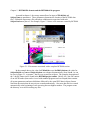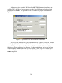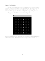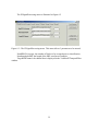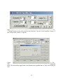
1
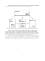
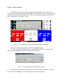
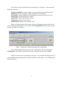
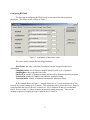
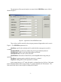
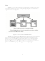
Preface
BCI2000 is a system of four modules that are independently executable programs. They
are described in detail in two documents: outline.pdf and specific.pdf. An overview of their
organization can be seen in Figure P.1.
Figure P.1. Overview of the four BCI2000 modules.
The EEG source module acquires EEG data from the A/D convertor, stores it to disk, and
passes a sub-set of the EEG signal to the signal processing module. The signal processing
performs a series of cascaded filtering operations that result in a cursor-control signal that is
passed to the application module. The application module controls the users’ task and the
appearance of the users’ screen. The operator module serves as a interface between the human
operator and the BCI2000 system by collecting parameters and displaying data.
1
The four modules of BCI2000 can be associated with a series of menus used to input the
parameters of the system. These associations are illustrated in Figure P.2.
Figure P.2- Association between the four modules and the various configuration menus.
The Source menu and the storage menu originate in the EEG source module and are
concerned with its’ operation. The signal processing module produces the MEMFiltering,
filtering and statistics menus. The application is configured by the UsrTask menu. Finally the
operator uses the Visualize and System menus. While the visualize menu actually originates in
the three other modules it is concerned with the operators’ data display function.
In order to work properly, the BCI2000 system must have values set for the parameters
found in these menus. The system starts with default values. Changes may be made manually
be the operator or by reading in parameter files. Parameter files may be read in as complete lists
of all parameters or as parameter file fragments that modify only a subset of the parameters.
2
Chapter 1- Basic Operation
BCI2000 Consists of four separate programs that run simultaneously. These are the
operator, data acquisition, signal processing, and the user application. All four programs must be
started and connected for the system to work. They may be started individually, in which case
they will appear as seen in Figure 1 below.
Figure 1. Screen appearance of the four programs launched manually.
In order to connect the programs click on the 3 Connect buttons.
Alternatively, the four programs may be launched from a batch file, in which case all
programs except the operator may be invisible, as seen in Figure 2.
Figure 2. Screen appearance of the operator program.
BCI2000 has many parameters that need to be entered for proper operation. In order to
do so click on the Config button. The configuration menus will then appear.
3
One appearance of the configuration menu is shown in Figure 3. It is important to note
that the appearance of these menus is dynamic in the sense that they depend upon the features
included in the current version of BCI2000.
Figure 3. Appearance of the configuration menu.
Note the tabs at the top of the menu. The particular menu shown is that associated with
the storage tab. There are 8 menu tabs shown in Figure 3. These are:
Visualize- controls the data shown to the human operator during operation.
MEMFilter- parameters of AR spectral analysis.
Source- parameters of data acquisition.
UsrTask- parameters of the subjects’ task.
Statistics- parameters that control automatic adaptive adjustments.
Storage- parameters that control naming of data files.
System- parameters that control communication between the four programs.
Filtering- parameters that control signal processing.
4
Each of these menus can be selected by clicking on the corresponding tab. Also note that
the menu shown in Figure 3 shows four additional buttons on the right hand side. These are:
Save Parameters- stores parameters in a file.
Load Parameters- inputs parameters from a file.
Configure Save- provides selection of parameters that will not be saved to parameter
file.
Configure Load- provides selection of parameters that will not be read from parameter
file.
If the system has been parameterized and the results has been saved in a file, system
operation is relatively simple. Just click on the Load Parameter button and the menu shown in
Figure 4 will appear.
Figure 4. The Load Parameter menu.
The file containing the preselected parameters can then be loaded. Then
parameterization of BCI2000 is completed by adding the storage parameters.
5
Click on the storage tab and the Storage menu (Figure 3) will appear. This contains the
following parameters:
AutoIncrementRunNo- controls whether or not run number automatically advances.
FileInitials- the disk and directory where the data files will be stored.
SavePrmFile- controls whether or not the parameter file used for each run is saved.
StorageTime- time when data file is created.
SubjectName- initials identifying the subject.
SubjectRun- number of the current run.
SubjectSession- number of the current session.
When al of these parameters have proper values the Configuration menu can be closed
(click on X in upper hand corner). Next click on the Set Configuration button and the operator
program will appear as in Figure 5.
Figure 5. Appearance of operator program after configuration.
Notice that the Start button has become bold. This happens only after clicking Set
Configuration. The system is ready and the session will begin when you click on Start.
When the system starts several displays will appear. The particular data displays that are
present will depend upon the parameters selected from the Visualize menu. One configuration is
shown in Figure 6.
6
Figure 6. Appearance of BCI2000 during operation.
Figure 6 shows a configuration in which the parameters VisualizeSource and
VisualizeTemporalFilter have been selected. Also note that the Start button has changed to a
Suspend button. Clicking on the Suspend button will halt operation.
If you are creating a new parameter file, several of the Configuration menus will need to
be dealt with. There are two ways of doing this. One way is to enter all parameters by hand.
Another way is to partially configure the system by using parameter file fragments. For
example, the menu shown in Figure 4 lists several parameter files such as 4bars.prm and
dualmonitor.prm. 4bars.prm contains only those parameters necessary to configure the
system for a 4 target task. dualmonitor.prm contains only those parameters necessary to place
the users monitor on the second video screen. These two parameter file fragments can be read in
succession. Since they are fragments, only those parameters that they include will be changed.
Thus, some of the work of configuring the system can be done with a series of standard
parameter file fragments.
7
Configuring BCI2000
The first step in configuring BCI2000 involves selection of the data acquisition
parameters. The Source menu is shown in Figure 7.
Figure 7. Appearance of the source menu.
The source menu contains the following parameters:
BoardName- the name of the Data Translation board as it appears in the driver
information.
SampleBlockSize- size of data (per channel) block for each cycle of operation.
SamplingRate- data acquisition rate in Hz.
SoftwareCh- number of channels sampled (and stored) by the data acquisition program.
TransmitCh- number of channels transmitted to signal processing.
TransmitChList- identity of channels transmitted to signal processing.
In the example shown in Figure 7, a sample block size of 16 and a sampling rate of 160
result in the system running at 10 cycles/sec. This means that data is processed every 1/10th of a
second and that the cursor will move 10 times/sec. All 64 channels of data are recorded and
stored. However only 10 of these channels are passed to signal processing. These are the
channels required to compute the large Laplacian for CP3 and C4.
8
The parameters of the spectral analysis are entered in the MEMFilter menu, which is
shown in Figure 8.
Figure 8. Appearance of the MEMFilter menu.
These values could be entered by the mem.prm parameter fragment that can be seen in
Figure 4. The MEMFilter parameters are:
deltaMem- specifies the resolution (in Hz) with which the autoregressive model is
evaluated.
MemBandWidth- specifies the width (in Hz) of the spectral bands produced.
MemDetrend- whether or not linear detrending is preformed.
MemModelOrder- the order of the AR model.
MemWindows- the number of data blocks (each SampleBlockSize long) used per
spectrum.
StartMem- beginning point at which the spectrum is evaluated.
StopMem- ending point at which spectrum is evaluated.
In the example shown, a 10th order AR model is evaluated from 0 to 50 Hz in 3 Hz bands.
Each 3 Hz band consists of the average of the ( 15 ) points evaluated at 0.2 Hz intervals. The
linear trend in the data is removed prior to fitting the AR model.
9
The parameters of the other parts of signal processing are accessed in the Filtering menu.
The appearance of the Filtering menu is shown in Figure 9.
Figure 9. Appearance of the Filtering menu.
The filtering menu has the following parameters:
AlignChannels- whether or not a linear interpolation is used to align channels in time
LR_A- Value of the intercept for horizontal (left/right) movement
LR_B- Value of the slope for horizontal movement
MaxChannels- maximum number of channels that can be handled by signal processing
MaxElement- maximum number of elements/channel that can be handled by signal
processing
MLR- matrix that defines the channels and frequencies that determine horizontal
movement
MUD- matrix that defines the channels and frequencies that determine vertical movement
10
NumControlSignals- number of control signals (up/down and right/left)
SourceChGain- list of gain values for each channel to convert A/D units to microVolts
SourceChOffset- list of intercept values to convert A/D units to microVolts
SpatialFilteredChannels- Number of spatial filter output channels
SpatialFilterKernal- Matrix that defines spatial filter transformation
UD_A- Value of the intercept for vertical (up/down) movement
UD_B- Value of the slope for vertical movement
There are several parameters (e.g., MUD,. SpatialFilteKernal) that have Edit Matrix and
Load Matrix options. The use of the Edit Matrix with the SpatialFilterKernal option is
illustrated in Figure 10. The vallues of the spatial filtering matrix can also be read in from a file
with the Load Matrix option.
Figure 10. The Edit Matrix option for the SpatialFilterKernal.
Notice that there are 10 columns and 2 rows in this example. The rows and columns can
be set by the set new matrix size button that appears in the top center of the menu. The 10
columns correspond to the 10 TransmitCh values of the source menu. That is, in the example
shown previously in Figure 7, the source menu specified that 10 channels are sent to signal
processing. These correspond to the columns of the spatial filtering matrix. In the current
example, the parameter SpatialFilteredChannels is 2. This corresponds to the rows of the
spatial filtering matrix and corresponds to the number of channels that are the output of the
spatial filtering operation. This will then be the number of channels input to spectral analysis
(MEMFilter) and the class filters (MUD and MLR). Thus, there is an interdependence between
some of the parameters. In this example, TransmitCh (from the source menu ) corresponds to
the columns of the spatial filter matrix (from the Filtering menu) as well as the number of
elements in SourceChGain and SourceChOffset (also from the Filtering menu).
11
The Edit Matrix option from the horizontal class filter (MUD) is illustrated in Figure 11
(note that MUD stands for Matrix Up Down).
Figure 11. Edit Matrix for MUD when ClassMode = 1.
In the example shown in Figure 11, there are 2 rows and 3 columns. When the variable
ClassMode is = 1 then 3 columns are required. The 2 rows correspond to two input features
from the spectral analysis. The 3 columns contain information that selects the features and
weights associated with these features. Column 1 specifies the SpatialFilteredChannel and
column 2 specifies the spectral bin associated with the first component of the feature. Column 3
specifies the SpatialFilteredChannel. Column 3 specifies the weight of the feature. The control
signal for vertical movement would then be the weighted sum of the feature specified in
12
Figure 11b. Edit Matrix option when ClassMode= 2.
In the example shown in Figure 11b, ClassMode= 2 has been entered and 2 rows and 5 columns
appear. This indicates that the product of two features will be computed for each row. When 0
appears in columns 3 and 4 only one feature is used for that row. When non-zero indices specify
a second component (columns 3 and 4 ) this is multiplied by the first component (column 1 and 2
). This provides a means of generating interaction terms (products). This example illustrates
another interdependence in the system. The MUD matrix must match the SpatialFilterKernal
in the sense that there must be SpatialFilteredChannels and spectral bins corresponding to the
features specified in MUD. A full list of system dependencies will be presented in Table 1.1
below.
13
The Statistics menu provides for input of parameters that control automatic adaptation of
the system and is shown in Figure 12.
Figure 12. Appearance of the statistics menu.
The statistics parameters are:
BaselineClg- matrix for selection of baseline used for cursor gain and intercept control.
DesiredPixelsPerSec- rate of vertical cursor movement in pixels per second.
InterceptControl- whether or not the intercept for vertical cursor movement is adapted.
InterceptLength- length of window for intercept adaptation.
InterceptProportion- proportion of the mean of the control signal used as the intercept.
LinTrendLrnRt- rate at which the linear trend of proportion correct is adjusted.
QuadTrendLrnRt- rate at which the quadratic trend of proportion correct is adjusted.
TrendControl- whether or not the proportion correct over target position is adjusted.
TrendWinLth- length of running average over which trend in proportion correct as
computed.
WeightControl- controls use of online adaptation of classifier weights. 0 for no use, 1
for compute but do not use and 2 for use on-line.
WtLrnRt- this is the learning rate used by the LMS-based on-line adaptive classifier
14
The Edit Matrix option for BaselineClg is shown in Figure 13.
Figure 13. The Edit Matrix option of BaselineClg..
In the example shown there are 4 rows and 4 columns. The example is for a task with 4
targets (see UsrTask below). The data used for adaptation of cursor movement parameters will
be taken from the four TargetCode values shown when the value of Feedback is 1.
15
The UsrTask menu provides for input of the parameters that control the users’ task and is
shown in Figure 14.
Figure 14. Appearance of the UsrTask menu.
The UsrTask menu has the following parameters:
CursorSize- the size of the cursor in pixels (pixel size depends on screen settings).
ITIDuration- the duration of the period between trials (in units of cursor updates).
NumberTargets- number of alternative targets on the user screen.
PreTrialPause- the duraion of initial target appearance without cursor present
RestingPeriod- mode where baseline is taken (rather than target presentations).
RewardDuration- duration that trial outcome is displayed (in cursor update units).
TargetWidth- width of targets in pixels
16
WinHeight- height of user window in pixels
WinWidth- width of user window in pixels.
WinXpos- horizontal position of upper left user window (in pixels).
WinYpos- vertical position of upper left user window (in pixels).
The appearance of the users’ screen is shown in Figure 15.
Figure 15 Appearance of Users’ screen. Note the cursor and the target.
17
The Visualize menu provides for entering parameters that control the run-time display of
data and is shown in Figure 16.
Figure 16. Appearance of the Visualize menu..
The Visualize menu has the following parameters:
SourceMax- maximum expected value of the source (raw data) display.
SourceMin- minimum expected value of the source display (these values scale the
display).
VisualizeCalibration- whether or not the results of the calibration are shown.
VisualizeClassFiltering- whether or not the results of the classifier are shown
VisualizeNormalFiltering- whether or not the results of the normalizer are shown
VisualizeSource- whether or not the raw data are shown
VisualizeSpatialFiltering- whether or not the results of spatial filtering are shown.
VisualizeStatFiltering- whether or not the proportion correct by targets is shown
VisualizeTemporalFiltering- whether or not the results of the spectral analysis are
shown
18
The System menu displays system configuration data and is shown in Figure 17. These
values are not normally changed by the operator and should not be saved or loaded.
Figure 17. Appearance of the System menu.
These values can be omitted from saving and loading in the parameter file by clicking on
these buttons on the right side of the screen as illustrated in Figure 18.
Figure 18. Appearance of the Config Load menu illustrating omission of system parameters.
19
Table 1.1. List of BCI2000 parameter interdependencies. Note that all parameters in the
same group must match.
Parameter
Menu
Type
Group
TransmitCh
Source
numeric
A
SourceChGain
Filtering
number of elements in list
A
SourceChOffset
Filtering
number ofelements in list
A
SpatialFilteringKernal
Filtering
matrix - number of columns
A
SpatialFilteringKernal
Filtering
matrix- number of rows
B
SpatialFilteringChannel
s
Filtering
numeric
B
MUD
Filtering
matrix- number of columns
B
MLR
Filtering
matrix- number of columns
B
StopMem-StartMem /
membandwidth
MEMFilter
computed- number of
spectral bins
C
MUD
Filtering
matrix- number of rows
C
MLR
Filtering
matrix- number of rows
C
20
Chapter 2- The screening program
As noted earlier, BCI2000 consists of four separate programs that run simulaneously.
These are the operator, data acquisition, signal processing, and the user application. Different
versions of these programs can be run with the BCI2000 system. One alternative user
application is the screening program. This can be launched manually or with a batch file, as
discussed in the beginning of chapter 1. In either case, the appearance of the various menus are
similar with the exception of the UsrTask menu. When the screening program is run, the
UsrTask menu appears as shown in Figure 2.1.
Figure 2.1. Appearance of the UsrTask menu when running the screening program.
21
Note that most of the parameters remain unchanged with the exception of the addition of
TargetOrientation and TargetDuration. Also, parameters referring to the cursor are not
present.
The screening program has no cursor or cursor movement. Hence the duration of
screening trials is determined by the TargetDuration parameter. In addition, the target
appearance for the screening program is different. Figure 2.2 shows the user screen for the
screening
program.
Figure 2.2. Appearance of the user screen with the screening program.
Note that the target appears on the bottom of the screen. Whereas the initial user task had
targets aligned along the right edge of the users’ screen, the screen task has targets on the top and
bottom edge of the Users’screen (for TargetOrientation = 1) or on the left and right edges of the
Users’screen (for TargetOrientation= 2).
22
Chapter 3- The FIR program.
As we saw in chapter 2, different versions of the four separate programs comprising
BCI2000 can be used interchangeably. An example of an alternative signal processing program
is the FIRProcessing program. The use of digital filters (e.g. fixed-impulse, or FIR) is an
allternative to AR-based spectral analysis. Most menus are identical with the FIRProcessing
program. The exception is that the MEMFilter menu is replaced with a FIRFiltering menu.
The appearance of the FIRFiltering menu is shown in Figure 3.1.
Figure 3.1. Appearance of the FIRFiltering menu.
The FIRFiltering menu has the following parameters:
FIRDetrend- determines whether or not linear detrending is performed.
FIRFilteredChannels- the number of channels that will be filtered
FIRFilterKernal- a matrix of the FIR filter weights.
FIRWindows- number of data blocks that are combined at each filtering cycle.
Intergation- determines whether the mean ( 0 ) or RMS (1) value is output.
During normal operation the FIRFilterKernal is loaded with the Load Matrix option.
It can be produced by running the program MakeFir.
23
The MakeFir program produces a matrix output that can be read directly into BCI2000
with the Load Matrix option. The appearance of the MakeFir main window is shown in Figure
3.2.
Figure 3.2. Appearance of the MakeFir menu.
The desired parameters are selected for each filter and then MakeCoeff is depressed.
Each time MakeCoeff is depressed, filter coefficients determined by the current parameter
settings are produced and the Filter # counter is advanced. Figure 3.3 shows the window
displayed when ViewSpectrum is depressed.
24
Figure 3.2. Appearance of the ViewSpectrum menu.
Figure 3.2 shows an example of the band-pass characteristics of three 32nd order filters
centered at 0, 11 and 22 Hz. If the operator is satisfied with these characteristics a file name can
be selected with the OutFile button and created by depressing the SaveCoff button. Note that
the MakeFir menu has a Bandwidth option. The bandwidth will not be less than the value
selected, but the width is also limited by the filter order.
25
Chapter 4- The Calibgen program
As noted in chapter 1, the BCI2000 Source menu has the parameter TransmitCh and the
parameter list TransmitChList that specify which channels are sent from the EEG source
program to signal processing. The Filtering menu has the parameter lists SourceChGain and
SourceChOffset that provide information for calibration of these same channels. All of these
parameters can be generated from the Calibgen program.
The Calibgen program takes as input a BCI2000 data file containing a calibration signal.
The user selects the desired channels. The output is a BCI2000 parameter file fragment. The
initial appearance of the Calibgen program is shown in Figure 4.1.
Figure 4.1 Appearance of the Calibgen main window.
Click on the SelectInput button and the next window appears as shown in Figure 4.2.
Figure 4.2. The Calibgen input window.
26
Next select the output file.
Figure 4.3. Appearance of the output window.
If fewer than 64 channels are to be included in the output (parameter file fragment) click
on the Enable Channellist box and enter the list into the list box. Then click on go. The
selected file name will contain a BCI2000 parameter file fragment similar to that shown below:
Parameter File Fragment Calib.prm Generated by Calibgen
Filtering floatlist SourceChOffset= 5 245 -202 -86 -155 17 0 -500 500 // offset for channels in A/D units
Filtering floatlist SourceChGain= 5 0.00802 0.00806 0.00797 0.00805 0.00807 0.033 -500 500 // gain for each
channel)
Source int TransmitCh= 5 4 1 128 // the number of transmitted channels
Source intlist TransmitChList= 5 9 33 41 49 11 1 1 128 // list of transmitted channels
In this example only 5 channels were selected (appropriate for a C3 Large Laplacian).
This file can now be read into BCI2000 with the Load Parameters option.
27
Chapter 5 - BCI2000 file formats and the BCI2000toGab program
As noted in chapter 1, the storage menu allows for input of FileInitials and
SubjectName as parameters. These parameters determine the location of the BCI2000 data
files. FileInitials represents a file path where subdirectories associated with each
SubjectSession are placed. For example, Figure 5.1 shows a file structure created by BCI2000.
Figure 5.1- File structure associated with a complete BCI2000 session.
In the example shown, the value for FileInitials was c:\bci2001\data\em, the value for
SubjectInitials was em and SubjectSession was advanced (automatically) from 1 to 8. As can
be seen in Figure 5.1, a separate *.dat file was created for each run. The complete description of
the *.dat file format can be found in the BCI2000 project outline. Briefly, the *.dat file consists
of an ASCII header (that can be viewed with standard programs such as notepad) that contains
all system parameters and state definitions followed by the actual EEG data in binary format.
Note that directories that do not exist are created automatically. Also new data files are created
automatically at the beginning of each run using the next highest number. The program scans
the directory to avoid overwriting any files.
28
Two additional files are presently created. The *.apl file contains a brief summary of the
subjects’ performance as illustrated below:
emS203.apl
Thu Sep 13 12:42:55 2001
Run 1 Hits= 30 Total= 32 Percent= 93.75
Number of Targets= 2
Bits= 21.21
Time Passed (sec)= 180.06
..........................................................
Run 2 Hits= 26 Total= 32 Percent= 81.25
Number of Targets= 3
Bits= 22.44
Time Passed (sec)= 180.06
..........................................................
Run 3 Hits= 24 Total= 32 Percent= 75.00
Number of Targets= 4
Bits= 25.36
Time Passed (sec)= 180.06
..........................................................
Run 4 Hits= 27 Total= 32 Percent= 84.38
Number of Targets= 4
Bits= 36.07
Time Passed (sec)= 180.05
..........................................................
This example is truncated at 4 runs for the sake of saving space. In addition, a *.sta file
is created. This is the output of the statistics filter and provides trial-by-trial information
concerning dynamic adaptation of BCI2000.
29
At the present time a complete Windows-based BCI2000 data analysis package is not
available. The *.dat files can be converted to the older *.raw file format and analyzed with
programs such as memm. The appearance of the BCT2000toGab program is illustrated in
Figure 5.2.
Figure 5.2- Appearance of the BCI2000toGab main window.
Any one of the *.dat (BCI2000) files in the subdirectory of interest is selected. Next the
desired output (GAB) file is selected. The Calibration Parameter File is selected (64 channel
output of Calibgen- see chapter 4). When the Load List button is clicked the first and last run
found in the selected subdirectory are displayed. In the example shown, the first run has been
changed manually from the initial value of 1 to a value of 3. Thus, only the 3rd run on will be
converted. When the convert button is clicked the GAB File is created as output. This file is
memm compatible.
30
Chapter 6 - The P300 Speller
Use of the programs P3Signalprocessing.exe and P3Speller.exe in conjunction with data
acquisition and operator modules allows for use of the P300 Speller. This configuration has the
Visualize, Source, Statistics, Storage, System and Filtering menus as discussed earlier. In
addition, the P300 configuration also includes the P3SignalProcessing and P3Speller menus.
The appearance of the P300 user screen is shown in Figure 6.1
Figure 6.1 - The P300 User screen. Each of the 6 rows and columns are flashed (highlighted) in
a block-randomized order. When N blocks have been completed a letter is selected.
31
The P3SignalProcessing menu is illustrated in Figure 6.2
Figure 6.2 - The P3SignalProcessing menu. This menu allows 3 parameters to be entered:
NumERPsToAverage- the number of blocks to be averaged prior to classification.
NumSamplesInERP- the length of the ERP waveform in samples.
TargetERPChannel- the channel that is displayed in the VisualizeP3TemporalFilter
window.
32
The P3Speller Menu is illustrated in Figure 6.3
Figure 6.3 The P3Speller menu allows for entry of:
BackgroundColor - Hex values for the background of the User’s screen. All 0s is black.
In positions 3-4 more Blue is added as the value increases. The value in 5-6 adds green and the
value in 7-8 adds red.
NumberOfSequences - The number of presentations per classification. Currently this
must be an integer multiple of the value of NumERPsToAverage in the P3SignalProcessing
menu.
OffTime - number of system cycles that the highlight is off.
OnlineMode - free spelling
OnTime - number of system cycles that the highlight is on
33
PostSetInterval- delay at end of set
PreSetInterval- delay at beginning of set
StatusBarSize- size of bar at top of user screen showing letters to spell and letters spelled
StatusBarTextHeight- size of text in bar at top of screen
TargetDefinitionFile- full path of file that defines selections on the screen
TargetHeight- height of area in which each letter appears
TargetTextHeight- height of the text in the target area
TargetWidth- width of area in which each letter appears
TextColor- hex bit pattern (BGR) that defines color of targets
TextColorIntensified- hex bit pattern that defines change when row/columns flash
TextToSpell- word(s) that subject must spell
34
Additional considerations:
Certain other parameters, covered in previous chapters, must be dealt with.
in the Filtering menu, values for MUD must be set to allow for classification of the P300. This
works as covered previously except that the column 2 values are time points rather than
frequency bins. For example, Figure 6.4 shows one configuration.
Figure 6.4 One possible configuration of MUD (from Filtering menu).
In this configuration, the values in column 1 indicate that signal 2 is being used for P300
classification. The values in column 2 indicate that time points 32-36 are used for classification.
Finally, the values in column 3 indicate that all points are given equal weights (1).
Also, in the Filtering menu, the values of UD_A should be 0 and UD_B should be 10.
Chapter 7. Maxifred.exe
35
Maxifred.exe is a utility that can be used for visual inspection of BCI2000 data files. It provides
for a simple “polygraph” type view of short segments of data. Upon clicking on the programs
icon the following form appears.
Figure 7.1- The
form.
initial Maxifred
Click on “Let’s kick it!!” and proceed to the main form.
36
Figu
re
7.2. The main Maxifred. Click on the “File” button in the upper left hand of the form and the
open file dialog appears.
Figure 7.3.
The open file
dialog.
Select the
BCI2000 data file to view. When the main form appears select “GO” on the upper right of the
form
37
Figure 7.4. Display of BCI2000 data. Note the controls at the top of the form. The number of
channels and points to display can be selected. The “Jump To..” button alows the user to
advance to a selected trial within the BCI2000 run. Scaling controls the Y-axis amplitude of the
EEG signals. There are also arrow buttons that control movement through the record. To the
immediate left of the “GO” button is a list of State codes. This list is read from the data file and
its contents will vary. Note that in the example “TargetCode” has been checked. This causes
any change in the value of the state “TargetCode” to be marked on the record. Also note that the
time within the run appears on the bottom of the record.
38
Figu
re
7.5 Magnification of some of the controls from Maxifred. Note the “Edit Channellist” button. If
this is selected the form in 7.6 appears.
Figure
7.6. The
Edit
Channellist
form. This menu allows application of the Common Average Reference (CAR) to the displayed
data.
39
EEG Samples from Maxifred.
Figure 7.7 - EEG Sample that illustrates a pair of eye blinks that are apparent on channels fp1af4 (22-28). Note that the eyeblinks affect all channels to some extent but are most pronounced
in the front of the head (near the eyes).
40
Figure 7.8 -. EMG activity that is particularly pronounced on channels af7 and fp1 (25 and 22).
Also note the alpha-band spindles present throughout many channels (see Figure 3)..
.
Figure 7.9 - Alpha spindles
from Figure 2.
41
Figure 7.10 - EEG sample showing a large EKG effect. Note the regularly occurring, small
upward deflection2 on all channels. There is also a single eyeblink.
42