Download APECSgui Installation Guide and User Manual Version 1.0 March

APECSgui
Installation Guide and User Manual
Version 1.0
March 31, 2012
1. Introduction
APECSgui is a graphical user interface for using advanced signal processing, machine learning and
statistical methods to create EEG-based models of cognitive states. The models are based on extensive
research by PDT scientists and their partners1 on developing algorithms for Advanced Physiological
Estimation of Cognitive Status or APECS. APECSgui allows non-experts, who are generally familiar with
EEG signal processing and human cognition to design, train, validate, and test APECS models. It also
allows users to export model parameters for real-time estimation of cognitive status using specialpurpose applications for BCI2000 (www.bci2000.org), such as the PDT Gaze Contingency Task.
2. System Requirements
MATLAB Version 7.10 (R2010b)2 or higher is a pre-requisite for using APECSgui and must be installed or
accessible from a server on the computer you will use to run APECSgui. For standard functions, APECSgui
does not require any MATLAB toolboxes3.
Generally, the system requirements for MATLAB (see www.mathworks.com) will determine the
minimum requirements for using APECSgui. These include 1) any Intel or AMD x86 processor supporting
SSE2 instruction set, 2) 1 GB disk space for MATLAB only, 3–4 GB disk space for a typical installation,
1024 MB RAM minimum, at least 2048 MB RAM recommended. However, for working with most realworld EEG data sets, we recommend a system with at least two high-speed CPUs (> 2 GHz), 4 GB of
RAM, and 250 GB of disk space. Performance of the minimal system may run into “out of memory”
errors for large EEG data sets. To avoid such errors and for noticeably faster performance, we
recommend a system with four 64-bit AMD or Intel processors, 8 GB of RAM and a hard disk drive
running at 7200 RPM or an SSD disk. We also recommend a dedicated graphics processor with a
resolution of at least 1280 x 1024 pixels for displaying high resolution graphs of data, features, and
models.
APECSgui also requires use of the open-source N-way4 subroutines for efficient calculation of multiway
methods such as PARAFAC (parallel factor analysis) or N-PLS (multiway partial least squares regression).
The current version (Version 3.1) is included in this APECSgui installation package.
We have tested APECSgui on Microsoft Windows operating systems and confirmed operation on
Windows XP SP3, Windows Vista Home Premium SP2, and Windows 7 Home Premium SP1, and Mac
OSX. In principle, any operating system that supports MATLAB, such as UNIX, or Linux, should support
APECSgui, but we have not tested APECSgui with these systems.
We designed APECSgui to provide model parameters for the PDT EEtrac system. EEtrac is a unique
hardware and software system for doing experiments in which EEG and eye-movements are
simultaneously recorded, and in which task events and feedback may be contingent on EEG and eyemovement features estimated in real time. The PDT GazeContingencyTask, for example, allows for
experiments’ in which the location of stimuli on a display may be contingent on instantaneous gaze and
concurrent EEG-based estimates of mental fatigue or mental workload, which are estimated using
APECSgui model parameters. EEtrac and the GazeContingencyTask are built on the Open Source BCI2000
framework for brain-computer interface development5. To use APECSgui model parameters with EEtrac
you must install the free BCI2000 framework on the computer that you will use to run EEtrac. MATLAB
and APECSgui do not need to be installed on the EEtrac computer. A separate document explains the
hardware and software requirements for EEtrac and provides instructions for running the PDT
GazeContingencyTask6. In Section 5 (Using APECSgui) we explain how to export APECSgui model
parameters for use with EEtrac and BCI2000.
3. Installing APECSgui
To install APECSgui, you must choose a root folder, which will contain required application code, raw
data, processed data, computed features, results, and graphs. To work with typical EEG and cognition
experiments, the root folder should be on a device that has at least 30 GB of available file storage space.
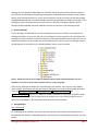
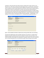
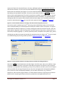
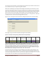
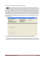
After choosing or creating the root folder, extract the contents of the APECSgui code package
(APECSguiCodePackage.zip) in the root folder. This will create a default folder tree containing codes and
other folders for storage of data and other file types consisting of eight subfolders: Customized-M-files,
Filters, M-files, N-way, ParameterFiles, Results and Weights_BCI2000_xls (Figure 1). The APECSgui codes
do not use much space, so if you will use APECSgui for various unrelated analyses, we recommend
creating a separate root folder for each analysis. For example, if your study is about Cognitive Fatigue
Study 1, you may create a root folder such as “F:\Analyses\Cognitive-Fatigue-Study-1” on hard disk F:
and install APECSgui there.
APECSgui User Manual Version 1.0.1
Page 2
Although you can change the Data folder tree arbitrarily, we do not advise this because some parts of
the code rely on default paths for loading and saving files. The APECSgui Data Package includes sample
data for tests or demonstrations. To use the sample data sets, extract the contents of the data package
(APECSguiDataPackage.zip) in the Data subfolder located in the APECSgui root folder you created. To use
APECSgui to analyze your own data, you must install your data files in the Data subfolder. We will
describe the data subfolder and other subfolders and how to use them in the following sections.
4. Starting APECSgui
To start APECSgui start MATLAB and set the working directory to the root folder you created for the
APECSgui installation. Then run the start-up script APECSgui.m, which should be in the root folder if the
APECSgui is properly installed. To maintain consistency with required folders for data and other files, we
recommend staying in the root folder over the MATLAB session in which you will use APECSgui. At startup APECSgui will set the paths to all required subfolders relative to the root folder.
Figure 1. Default structure of the root folder for APECSgui, which contains required application code, and
subfolders for raw data, processed data, computed features, results, and graphs.
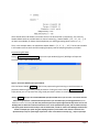
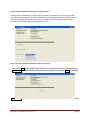
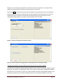
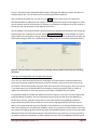
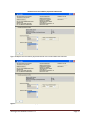
After starting, APECSgui will display the main APECSgui input window. There are four main modules,
which create a pipeline for processing data from its raw format to running an APECS model application.
These are 1. PreProcess Module , 2. Feature Module , 3. TrainValTest Module and
4. Application Module (Figure 2). An additional module is available for optionally saving APECS model
weights to use within PDT real-time applications for BCI2000, such as the GazeContingencyTask. An
option for saving weights in Microsoft Office Excel file format is also available.
5. Using APECSgui
Raw Data Format
To use APECSgui with your data, you must create raw data files with a format that APECSgui can use.
The APECSgui raw data file is a MATLAB data file (.mat file) which must contain two structures: dat and
header.
APECSgui User Manual Version 1.0.1
Page 3
Figure 2. Main input window for APECSgui, showing options for 1) pre-processing data, 2) feature extraction, 3)
model training, validation and testing, 4) applications of models. A separate Save weights option is available for
generating real-time model weights to use within the PDT EEtrac system6, such as the GazeContigencyTask. The
EEtrac system is built around the general purpose BCI2000 framework for brain-computer interface
development. The Save weights option also allows you to save model weights into a Microsoft Office Excel file.
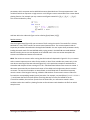
The dat and header structures must be created and saved in each data file you wish to analyze and
stored in the Data/RawData subfolder. The dat structure contains two matrices, dat.X and dat.Y, where
X has dimensions of samples x electrodes and Y has dimensions of samples x events data7. For example,
consider the case of recording 166400 samples of EEG from 32 electrodes and event information (e.g.,
stimulus onset times, response times, hits, misses, etc.) during an experiment. The dat structure for
these data would have the form:
.
Both X and Y can be matrices or arrays. If no events are recorded, Y should be defined as a vector with
identical values, e.g., all equal to 1.
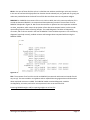
The header structure must contain the five variables: Xsize, Ysize, Xlabels, sampleFreq, and
sampleFreqUnit. These variables provide data dimensions and sampling parameters8. For the prior
example, a valid header structure could be
APECSgui User Manual Version 1.0.1
Page 4
where header.Xsize and header.Ysize reflect the sizes of dat.X and dat.Y, respectively. The cell array
header.Xlabels holds the variable labels or channel names (e.g., header.Xlabels = {‘F3’, ‘F4’ , ‘C3’ ….}). If
no labels are available, for better data manipulation, we advise generating labels such as 1, 2, 3, … .
Then, in the example above, we would have header.Xlabels = {‘1’, ‘2’, ‘3’, …, ‘32’}. The last two variables
in the header structure store the EEG sampling frequency and the sampling frequency unit label.
Preprocessing EEG Data
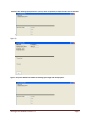
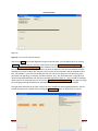
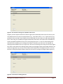
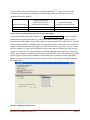
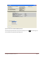
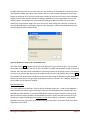
Clicking Step 1. PreProcess Module in the main input window (Figure 2) APECSgui will open the
PreProcess main input window (Figure 3).
Figure 3. PreProcess Module main input window.
Click the button labeled Add File to start a new preprocessing task starting or Load Parameters to
preprocess data using previously saved parameters. Clicking the button labeled Load Parameters
simply allows you to re-process files using saved parameters without re-entering parameters.
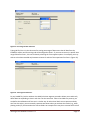
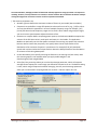
Clicking Add File will open the standard MATLAB Open file window where you can select a stored raw data file.
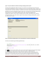
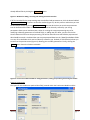
After selecting a data file a sub-window will open where you must define pre-processing parameters (Error!
Reference source not found.). The first two parameters pertain to epoch length and overlap. These serve to tell
APECSgui how to divide the continuous EEG series into a set of equal-duration epochs, with or without overlap.
You specify epoch duration and overlap in units of milliseconds, seconds or minutes and APECSgui calculates the
number of samples per epoch using the sampling frequency in the header. Note that for continuous nonepoched EEG you may set epoch length equal to the entire record with zero overlap (e.g., only one epoch per
APECSgui User Manual Version 1.0.1
Page 5
data file). After defining epoch parameters you may choose to optionally resample and filter the raw EEG data
(
Figure 5).
Figure 4. Preprocess Module sub-window for defining epoch length and overlap options.
APECSgui User Manual Version 1.0.1
Page 6
Figure 5. Preprocess Module sub-window for defining resampling and filter options.
Checking the box labeled Filter Data? will allow you to choose a file containing a filter structure that
works with the MATLAB filter.m function. Although you may store the filter file anywhere, we advise you
to keep filter files in the Filters subfolder. The filter file must contain standard design (dM) and filter (fM)
MATLAB filter structures. APECSgui will apply the filter with a zero phase shift, by forward and backward
filtering the data. This will effectively double the filter order. We provide a MATLAB m-file
example_filter_design.m, which contains examples of how to create a few different filters, with the
APECSgui installation in the Filters folder. Figure 6 shows example of loading a Bandstop filter saved in
the ./Filters/filter3.mat file.
Figure 6. An example of loading a filter file. File “\Filters\filter3.mat” represents a Bandstop filter.
This filter was created using the following MATLAB steps
Click OK to move to the next window, where you may select optional preprocessing parameters (Figure
7). Checking the box labeled Process Events? allows you to specify a MATLAB script for
processing/labeling events parameters, defined in dat.Y, within each epoch. Such scripts must be
written by the user (we advise you to store such scripts within the Customized-M-files folder). If you
define dat.Y as a vector of events then after epoching, PreProcess Module will create a new variable
APECSgui User Manual Version 1.0.1
Page 7
called datY, a matrix with dimensions number of epochs x samples within an epoch. However, if you
define dat.Y as a matrix (you may want to store more types of events, e.g. reaction time, correctness of
response, misses, etc.) then after epoching, PreProcess Module will create the structure datY.var{ch}.Y,
where ch indexes the columns of dat.Y and for each such column a matrix of the size number of epochs x
samples within an epoch is created from dat.Y. Therefore, you must process datY according to its
structure. datY is the only input variable for custom event-based processing code. Two output variables
must be stored, mainly a new vector with class-membership (say dY) and classLabel a vector with unique
class-membership values. We provide an example in which dat.Y is a vector indicating various workload
levels from which we wish to create three workload classes (low workload = -1, high workload = 1 and
undefined = 0). The script for this example script is in ./Customized-M-Files/setWorkloadLabels.m.
Figure 7. PreProcess Module sub-window for optional event processing, variable subsets, and re-referencing.
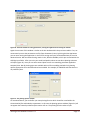
Checking the box labeled Select subset of variables? will pop up a sub-window for variable selection
(Figure 8). At this point we advise you to select all variables you may later use in the analysis. In the
Application Module representing the last step of the pipeline you will have the option arbitrarily select a
sub-set of variables actually used for final classification or explanatory analysis. In this way a necessity to
return to preprocessing step every time you decide to change a subset of variables will be avoided.
APECSgui User Manual Version 1.0.1
Page 8
Figure 8. PreProcess Module sub-window for variable selection.
Checking the box labeled Data re-referencing? will provide you options for re-referencing the EEG
electrode montage (Figure 9). Currently available options include average reference and the average
reference with global field power normalization. APECSgui re-references the montage using the
electrodes you selected in the variable selection step only.
Figure 9. PreProcess Module sub-window for data re-referencing.
After you click OK , the next window (Figure 10) allows you to correct defined values by clicking the button
Correct Values , or to finish definition of the parameters by clicking the button labeled Done .By clicking the
Correct Values button all selected parameters will be ignored and you will be moved to the initial parameters
APECSgui User Manual Version 1.0.1
Page 9
selection window
(
Figure 4).
Figure 10. Correct Values and Done window.
After clicking Done the window depicted in Figure 11 will be open. You can add a new file by clicking
Add File , or add file with the same set of parameters by clicking Add File (with existing param.) By
clicking Add File with existing param.) , a sub-window with a list of all currently selected files will open.
Here you need to select a file with parameters you want to duplicate. Then the next window will open
allowing you to select multiple files you can load. The same set of parameters will be assigned to these
files. For example, if you have several different files that you want to process in the same way (same
parameters for epoching, re-sampling, variables selection, etc.), you would start with a single file and
repeat all steps defined above until you get to window depicted in Figure 11. Now, instead of repeating
these steps for all remaining files you can click the Add File (with existing param.) button again to assign
the same preprocessing parameters for subsequent files. You may repeat this step as needed.
The right panel will allow you to check a list all currently loaded files and assigned parameters. You can
correct parameters for a specific file by clicking the Correct File button or delete a file or a set of
APECSgui User Manual Version 1.0.1
Page 10
already defined files by clicking the Delete File button.
Figure 11. Window for adding, correcting and deleting parameters and files.
If all files intended for the preprocessing step were defined and parameters set, click the button labeled
File Selection – Done! to continue to the next window (Figure 12). At this point we advise that you save
all selected parameters by clicking Save Parameters . We also advise that you save these parameters
into the ParameterFiles folder or its subfolders which can be arbitrarily created by you. Saving
parameters allows you to load them later, either for running the same preprocessing step or for
modifying or deleting parameters of selected file(s), or adding new files. Now, you can click the PreProcess Data which will start the preprocessing. You will be asked first into which folder preprocessed
data should be stored. It is advised that you save preprocessed data into the ./Data/EpochedData folder
or to any of its subfolders which can be arbitrarily created by you. Go Back (to File Selection) allows you
to return to the previous menu (Figure 11) allowing you to modify parameters. Finally, clicking the
Finish! button closes the PreProcess Module.
Figure 12. Pre-Process module window for saving parameters, running pre-processing and closing the module.
Features computation
The inputs for this module are epoched data file(s) created within the PreProccess Module and the
APECSgui User Manual Version 1.0.1
Page 11
outputs are file(s) with computed features. Currently, APECSgui implements computation of spectral
and coherence features. You can start the Feature Module by clicking the Step 2: Features Module
button within the APECSgui panel (Figure 2). As in the PreProcess Module, the main input window
described previously (Figure 3) will open. You can then select either a new file ( Add File ) of epoched
data or load an existing parameter file, which can be further modified. If you added a new file, the next
two windows will determine the type of computed features and its parameters. For spectral features,
APECSgui provides three power spectral density (PSD) estimates (Figure 13). The default method uses
the built-in MATLAB method fft.m; you may also choose optional methods pwelch.m and pmtm.m9.
Figure 13. Features Module window for selecting a PSD method and setting PSD parameters.
You need to specify a window type (none10, Hamming, Hann and Blackman) and a set of parameters
which are determined by the selected spectral method (this includes number of fft points, or length of
sub-windows for Welch’s method, etc.) Currently, APECSgui provides four spectrum formats. These are
power (power); log power in dB units (log_power); positive log power (log_power+), where positivity is
enforced by computing log10(p + 1), where p represents power; and square root of power (sqrt_power).
APECSgui also provides three optional methods for computing coherence (Figure 14) 11. These are based
on the MATLAB signal-processing toolbox procedures cpsd.m, mscohere.m and tfestimate.m.
Figure 14. Features Module window for selecting coherence methods and setting parameters.
After clicking OK the second parameters window (Figure 15) will be open. Here you can define a range
of frequencies for which power or coherence values will be computed. The format in which frequency
sub-bands are computed is also allowed (e.g. [4 16] [17 25]). However, we advise you to set this range as
wide as possible and covering all frequencies you may later investigate within the Application Module.
At any time later, within the Application Module, you can define sub-features, e.g., subsets of
frequencies, from this wide range of features. This will avoid the necessity of returning to the Features
Module and re-computing the features whenever you decide to investigate a different set of
APECSgui User Manual Version 1.0.1
Page 12
frequencies. By checking the box labeled Zero-mean prior spectra computation?, each epoch will be
separately centered (zero-mean) before computing power or coherence.
After clicking OK the final window of the Features Module will open allowing you to save parameters,
compute features and close the module (Figure 16). By clicking the Generate Features the routine for
computing features is evoked. At this point we recommend that you save feature file(s) into the
./Data/FeaturesData/ folder or to another named subfolder within this folder.
Figure 15. Frequency range definition and data centering.
Figure 16. The final window for saving parameters, computing features and closing the module.
Creating Sets for Model Training, Validation and Testing with the TrainValTest Module
The inputs for this module are feature data file(s) which you can combine into training, validation and/or
testing sets. The output is a single data file which is then used as an input within the Application Module
(described in the next section). Currently, the model validation step within the Application Module is not
implemented; however you can define a validation subset in the TrainValTest Module. As for other
APECSgui User Manual Version 1.0.1
Page 13
modules, you start the TrainValTest Module from the APECSgui panel (Figure 2) by clicking
Step 3: TrainValTest Module a window for adding files and loading parameters will open (same as in
Figure 3). After loading a new file containing the desired features the software automatically recognizes
if class membership labels are present or not and opens an appropriate menu. Currently, the Application
Module works with binary classification only.
First, we consider the case where class labels are present. For example, consider the example with
several workload levels, e.g. low workload = -1, high workload = 1 and undefined = 0, mentioned in the
PreProcess Module section. A window for selecting classes by label will open after you decide to use this
label information (Figure 17).
Figure 17. Window for defining number of class(es) and class labels when class labels are present in the data.
Because the classification methods of the Application Module must be binary in the present version of
APECSgui, you must remove one of the three classes. Say you want to discriminate low- and high
workload. Then eliminate Class 3 (undefined workload level = 0) by clearing its field, which sets the class
3 label equal to an empty string (Figure 18).
Figure 18. An example of eliminating a class by clearing its field (in this case Class 3).
Then after clicking OK a window for setting training, validation and test sets will open (Figure 19). At the
top of the window you can see which labels are present in the currently loaded file and which labels
APECSgui will use for this file. Note that you can update labels and classes if you add a new file with
different labels later.
APECSgui User Manual Version 1.0.1
Page 14
Figure 19. The window for setting Train, Validation and Test sets.
Suppose you have separate data files of EEG for high and low workload periods. Each file uses only one
class label because it has only one workload level (e.g. , class labels either -1 or 1). If the first file is low
workload, when you load it you will define the low workload class only. When you add a high workload
file in a later step, you will define the high workload class. Note that in the simple case of two different
classes separated into different files you can avoid using labels at all. In this case, after loading a file
with data of one condition, you can assign all the data in that file to one class only. For example, by
checking the box labeled Train set in Figure 19, a sub-menu for defining the training set will open (Figure
20). There are two options for defining classes either by percentage of points (Percentage of data) or by
time (Time segment). Say you want to use all data of the loaded file as training data of class 1. You can
do this by clicking Percentage of data to open the sub-menu for setting percentage of data (Figure 21).
Figure 20. A sub-menu for defining train sets.
APECSgui User Manual Version 1.0.1
Page 15
Figure 21. Percentage of data sub-menu.
Typing 100 for Class 1 in the sub-menu for setting percentage of data means that all data from the
loaded file will be used for training and will be assigned to Class 1. If you want to use only a specific time
range of data for Class 1, this can be done by selecting the Time segment option. For example, you may
wish to select data recorded only between minutes 12 and 14 of the experiment for Class 1 (Figure 22).
Figure 22. Time segment sub-menu.
For any loaded file, (with or without class labels) the time-segment procedure allows you to arbitrarily
define data corresponding to class 1 and class 2 at the same time. When class labels are present, you
can define the Validation and Test sets in a similar way. Or when class labels are not present and only
one Test class exists, you can manually separate two classes when you evaluate the results (e.g., when
plotting results) if you know when the classes divide. An example of this may be to contrast the first half
APECSgui User Manual Version 1.0.1
Page 16
of a session from the second half in a mental fatigue analysis. Note that you can define all three sets can
(Train, Validation and Test) in a single file using these methods.
When classes are defined by percentages of data, APECSgui automatically checks and warns you if the
overall sum exceeds 100%. However, the process is different when class labels are present (consistency
within a class is checked) than when class labels are not present (consistency within all data is checked).
When you define classes by percentages of data APECSgui uses the following procedure. When class
labels are not present and you might define percentages of data such as: training 10% class 1, 30% class
2; validation 5% class 1, 25% class 2, and testing 25% for all classes (
Figure 23). Then, starting from the first observation, APECSgui will split the file in consecutive blocks
with no gaps, using a total of 95% of the data and leaving 5% unused (Table 1).
Figure 23. An example of selecting training, validation and test set by percentages.
Training
Set
Class 1
10%
0%–10%
Training Set
Class 2
30%
10%–40%
Validation
Set
Class 1
5%
40%–45%
Validation Set
Class 2
25%
45% –70%
Test Set
(all classes)
25%
70%–95%
Unused
5%
95%–100%
Total
100%
100%
Table 1. Training, validation and tests sets defined by percentages of data in a single file. The percentages set in
Figure 23 are training=(10% class 1, 30% class 2); validation=(5% class 1, 25% class 2), and testing=25% for all
classes The percentages of the data in the first row (colored bars) follow these specifications, but the overall
percentages of data in the file are additive as shown in the second row. For example, Validation Set 1 begins at
40% of the data because Training Sets 1 and 2 were 10% + 30% = 40% of the data.
On the other hand, when class labels are present APECSgui uses the labels to split the data for a class
into sets in the order training, validation, and test. The presence of class labels takes precedence over
time and percentage splitting. That means if you define a time segment then APECSgui will use only data
with class labels within the segment that matching the defined class label for a set.
APECSgui User Manual Version 1.0.1
Page 17
Finally, if you check the box labeled Reshuffle samples? APECSgui will randomly permute the data prior
making any data split. This will destroy the time ordering of the data sequence.
After you define parameters for sets you can click Done! , which will bring you to the previously
described windows for adding files and setting or correcting parameters (Figure 11 and Figure 12). Note,
you can load the same file several times. For example, you could use one segment of the file to create a
training set, then use the whole file (all data) for the test set.
The last window is for saving parameters, generating training, validation and testing sets and closing the
module (Figure 24). Clicking on the button labeled Generate Data Sets will cause APECSgui to create a
single output file containing the training, validation and/or test sets that you requested. At this point we
recommend saving this file in the ./Data/TrainValTest folder or any of its arbitrarily named sub-folders.
Figure 24. The final window for saving parameters, generating training, validation and testing sets and closing
the module.
Creating and Testing Models with the Application Module
Up to now, you have been learning how to use APECSgui to preprocess data, compute features and
create sets for training, validation and testing. These are necessary steps to set up the structures you
will need to create and test models using your data. Now comes the interesting part, where you can see
if your data support an EEG-based model for estimating or classifying cognitive status, or simply to
explore the multivariate or multi-way structure of your data to help generate new models.
The Application Module provides four different procedures (Table 2). First, there are two unsupervised
learning modeling procedures: principal components analysis (PCA) and the multi-way PARAFAC, or
parallel factor analysis, method. Second, there are two supervised learning modeling procedures:
supervised-learning classification procedures: Kernel Partial Least Squares (KPLS) and multi-way PLS
(NPLS). The unsupervised and supervised methods can be divided into conventional folded analyses in
which some dimensions are combined or folded for analysis (e.g. frequency and electrode) or true multiway method of handling high-dimensional data. NPLS and PARAFAC operate on multi-array (tensor) data
while KPLS and PCA are methods operating on two-dimensional arrays (matrices). Currently, only KPLS
can perform nonlinear classification; all other methods are linear. (KPLS and PARAFAC methods served
APECSgui User Manual Version 1.0.1
Page 18
as key methods in the initial development of the APECS algorithms12,13,14. More recently the NPLS
method has proved useful for creating normative EEG-based models for classification of mental
workload and cognitive fatigue.)
Unsupervised Learning
(exploratory analysis or
Supervised Learning
dimensionality reduction)
(regression or classification)
Mathematical Structure
Folded (two-way)
PCA (principal components analysis) KPLS (kernel partial least squares)
Multi-way
PARAFAC (parallel factor analysis)
NPLS (N-way partial least squares)
Table 2. The four modeling methods offered by the Application Module.
In the main APECSgui input window (Figure 2) click Step 4. Application Module to open the initial file
and parameter specification window (e.g., Add File and Load Parameters, Figure 3). Again, as in the
previously described modules, you can load either an existing parameter file or add a new file. The input
for the Application Module is a single file with training and testing sets created within the TrainValTest
module. The software automatically recognizes if the structure is a multi-way array or a matrix. If more
than one variable (e.g., more than one EEG electrode) and more than one feature (e.g. more than one
frequency in the spectrum or coherence features) are used, APECSgui sets the multi-array structure by
default. You can suppress this option by checking the box labeled “no” next to the Run multi-way mode?
Option (Figure 25). Suppressing the default multi-way mode for array data will cause the Application
Module to concatenate all existing arrays into a matrix (samples x (all variables and features)) suitable
for folded analysis.
Figure 25. Switching off multi-way mode.
APECSgui User Manual Version 1.0.1
Page 19
As mentioned above, APECSgui provides for folded and multiway approaches using supervised or unsupervised
modeling. However, several parameters are common to all four methods. We can illustrate this with an example
of using NPLS (Figure 26. Parameters common to all four implemented methods.
). The common parameters are
 Number of factors defines the maximum number of factors in your model (latent variables)
 Frequencies to use defines a range of frequencies to be used in units of Hz, e.g., [4 6] for 4-6 Hz.
You may also define this parameter in terms of multiple frequency range. For example, [4 6]
[12 18] will select the two frequency ranges: 4-6 Hz and 12-18 Hz. When using multiple ranges,
you must insert a space between adjacent brackets of bins.
 Remove error samples. Before computing power spectra, the PreProcess Module computes the
variance of the EEG time series in each epoch and stores it in the header. The Application
Module can optionally use this information to exclude from training any epochs with variances
below or above criteria that you specify. You specify these criteria as percentiles of the
distribution of the variances of epochs in your data set. For example [5 95] will exclude all
epochs with variances below the 5th percentile or above the 95th percentile of the distribution
of variances of all training data epochs.
 Center data allows you to specify centering the features in the training set (zero-mean). Note
this centering option is not available when you apply models weights in the
GazeContingencyTask using BCI2000.
 Select freq. bins processing allows you to select the Average parameter, which will compute
averages across frequencies in each range you defined in Frequencies to use. The default setting
is none, which using all frequencies without averaging. You may use the Average parameter
when you are interested in analyzing bands such as theta = 4-8 Hz or alpha = 8-12 Hz.
APECSgui User Manual Version 1.0.1
Page 20
Figure 26. Parameters common to all four implemented methods.
Click OK to select parameters and another window will open where you may set two options, which are also
common to all modeling methods (Figure 27). Checking the box labeled Select subset of variables? allows you to
select a subset of variables for the model. Checking the box labeled Use customized plot function? allows you to
use a customized function to plot results. The process of selecting variables is the same as for the PreProcess
Module (Figure 8). Because the files you created in the TrainValTest Module contain all variables you kept in the
PreProcess Module, you can choose any subset of these variables when you run the Application Module. The
second option allows you to load a specific function for plotting results. We recommend saving such a function
(m-file) within the Customized-M-files. We will describe how to code such a function and the structure of the
output results below.
Figure 27. The second windows with two parameters common to all four implemented methods.
In addition parameters common to all methods you must specify additional parameters for the KPLS and
PARAFAC methods. For KPLS these are kernel type selection and the kernel function parameters. Two types of
APECSgui User Manual Version 1.0.1
Page 21
nonlinear kernel are available: polynomial and Gaussian.
Figure 28 depicts the case where polynomial kernel of the second order was selected.
Figure 28. Selection of the second order polynomial kernel for the KPLS method.
APECSgui User Manual Version 1.0.1
Page 22
Figure 29. Selection of the additional PARAFAC parameters.
After setting all required parameters for a particular method you can click OK which will bring you to
the last window of the Application Module (Figure 30).
APECSgui User Manual Version 1.0.1
Page 23
Figure 30. The final window for saving parameters, running the application and closing the module.
Again the structure of this window is similar to the last window within the previous modules. First, we
recommend you save the parameters to a file (Save Parameters). Next, by hitting the Run App button
you can start running the application. In the first file saving menu you will be asked where to save the
obtained results. We recommend saving results in the ./Results subfolder, which you can find within the
APECSgui root folder. After you train your model and predict values on test data a plotting sub-menu
will open (Figure 31). Here you can select several plots as well as a smoothing parameter applied to
temporal plots. Not all plotting types are available within all four modeling methods. Only plotting
options appropriate for a selected method are available. For example, for PARAFAC and PCA there are
no prediction plots.
Figure 31. The plotting options window.
As mentioned above, you can define your own plotting function which should be saved within the
Customized-M-files and loaded as a parameter. In this case the plotting options window (Figure 31) will
not appear but instead your defined plot routine will run. The plotting function takes to input
APECSgui User Manual Version 1.0.1
Page 24
parameters which are param and res MATLAB structures described next. The output parameter is the
variable hF which can represent a single name or a cell of figure names created within the custom based
plotting function. For example you may create several figures named hF ={‘fig_1’, ‘fig_2’, …., ‘fig_5’}.
This can be initialized by a loop
and later within the code each figure can be called as figure('Name',hF{f});
Results structure
After clicking Run App (Figure 30) you can name a file for saving the results. The results file is a binary
MATLAB file *.mat, which contains structures named param and res. The structure param holds all
important parameters selected within the Application Module. You can inspect these parameters can by
loading the saved results file into MATLAB and by typing param in the MATLAB command Window.
Results stored in the res structure depend on the method used. In the next section we explain this
structure and differences between the methods.
NPLS: The results res structure after running the NPLS method is depicted in Figure 32. First, res.meanX
and res.meanY represent mean values for the used X a Y data. These variables are present only in the
case where centering of data was selected (Figure 26). In this particular example we worked with 11
electrodes and 49 spectral lines creating an 11*49 = 539 dimensional X data mean vector res.meanX. Y
data were represented by one-dimensional vector of class labels and a single mean value is stored in
res.meanY. The next three variables res.YtrainFileInd, res.YvalFileInd and res.YtestFileInd represent
numeric vectors of the length of training, validation and test data. These numeric vectors index a file
from which a corresponding sample (epoch) was taken. For example, res.YtrainfileInd=[1 1 1 2 2 2 2 2 3 3
…] would mean that the first three epochs of training data are from the first loaded file in the
TrainValTest module, the next four epochs from the second file, etc. Information stored in these
variables can be then used for a plotting function to discriminate results based on the file from which
samples came.
APECSgui User Manual Version 1.0.1
Page 25
Figure 32. res structure for NPLS.
The next variables res.Xtrain, res.Xtest, res.Ytrain, and res.Ytest store the actual X and Y data used. If
centering was selected these data are zero-mean processed. In the depicted example we can see a
multi-array (multi-way) form of X data; particularly we can see that for training we used 637 epochs, 11
electrodes and 49 spectral lines. The same number of samples was used for testing in this case. In the
case of KPLS and PCA the variables res.Xtrain and res.Xtest would have the format of matrices of size
637 x 539 where electrodes and spectral lines are concatenated into a 539-dimensional vector.
res.Xfactors, res.Yfactors stores loadings (weights) of atoms (factors) computed by NPLS. In the example
above, 4 atoms were computed considering 3-way form of temporal x spatial x spectral components.
Therefore, res.Xfactrors{1} is a matrix of four 637-samples long temporal atoms. Similarly,
res.Xfactrors{2} is a matrix of four spatial atoms of size 11 corresponding to 11 selected electrodes and
finally res.Xfactrors{3} is a matrix of four spectral atoms representing weight vectors of spectral line
selected (in this case 49 spectral lines). res.Yfactors similarly represents Y space atoms (in our case Y
represents a class membership variable, therefore interpretation of res.Yfactors is not very meaningful.
Similar to res.Xfactors and res.Yfactors the next six variables res.Core, res.B, res.ypred, res.ssx, res.ssy,
and res.reg represent output variables of the npls.m routine from the N-way toolbox. You can learn
more about these variables by typing help npls within the MATLAB Command Window. Here we will
mention res.ypred which represents the training set predicted values of Y for one to number of selected
factors (components; in this case 4 factors). res.ypred is a matrix where each column represents
prediction values for a model consisting from one to the column number factors; i.e. the first column are
predicted values considering the first factor only, the second column considering both factors one and
two, etc. In the same way we compute predicted values for testing points. These are saved within the
res.ypred_test variable. Finally, res.T_test stores temporal components of testing set. Their linear
combination creates res.ypred_test. For better understanding of this prediction step you can type help
npred within the MATLAB Command Window.
APECSgui User Manual Version 1.0.1
Page 26
KPLS: In the case of linear KPLS the npls.m is called but now without considering a multi-way structure.
In the case of nonlinear KPLS (polynomial or Gaussian kernel selected) only res.ypred and res.ypred_test
values are provided because the kernel form of PLS does not allow access to component weights.
PARAFAC: For PARAFAC the structure of the res is similar to NPLS, but in this case no prediction of Y is
carried out because PARAFAC is an unsupervised data explanatory method. The structure of res for
PARAFAC is depicted in Figure 33. We can see that we have no Yfactors here. An important variable is
res.Xtest_tempAtom, which stores the projection of test data onto temporal atoms; in other words
representing temporal atoms of testing samples. The model diagnostic variables res.diagonality,
res.varian, and res.lev are stored in the case of PARAFAC. These variables represent a core consistency
diagnostic (type help corcond), residual variance and leverage values computed while running the
PARAFAC model.
Figure 33. res structure for PARAFAC.
PCA: The structure of res for PCA is similar to PARAFAC (now we work with matrices instead of multiway arrays). Two new variables res.eigValues and res.expVarPCA storing eigenvalues and information
about explained variance are added. The PARAFAC model associated diagnostic variables
res.diagonality, res.varian, and res.lev are not present in the res structure for PCA.
Extracting BCI2000 weights and/or exporting weights to an Excel file
APECSgui User Manual Version 1.0.1
Page 27
For NPLS and linear KPLS, you can save results in a text file which can be loaded as a classification filter
matrix within BCI2000. The output of this classifier will be a single variable indicating low versus high
fatigue (or workload). Once you have saved results of NPLS (or KPLS) that you want to save as BCI2000
weights, you can check the box labeled Save weights (BCI2000, xls) in the right bottom corner of the
APECSgui panel. This will open the initial window for loading the MATLAB results file. For all linear
models you can also export weight vectors to an Excel file. After loading the results file an option for
saving to BCI2000 and/or XLS will open (Figure 34). By checking the radio buttons BCI2000 and/or XLS
output weights formats are determined.
Figure 34. Window for saving results into BCI2000 format.
Then after clicking OK a window similar to the one depicted in Figure 35 will be open. You can select
the number of model factors you wish to save. By default the model with maximum number of factors is
selected. There are two formats of BCI2000 for referencing elements of the weight vectors (see BCI2000
tutorial). At the moment we recommend to use Bin format (select Bin radio button). After clicking OK –
Save weights! you will be asked to define name of the text file storing the BCI2000 classifier weights
and/or of an Excel file for storing weights. By default these files are stored in the ./Weights_BCI2000_xls
but the folder can be arbitrarily changed.
EEGLAB 2 Raw Data
First, open eeglab within MATLAB. Then by taking the following steps File -> Load Existing Database ->
select a dataset you wish to import. By doing this the structure ALLEEG becomes available within the
MATLAB Command Window. Type saveEEGLAB(ALLEEG, filename) where filename is a string of the
path and filename where the data in the MATLAB format will be saved. Data will be saved in the raw
data format needed for APECSgui (see Raw Data Format section above). If filename is omitted the
MATLAB file with the same name as the loaded data file will be saved into the same folder from which
eeglab data were loaded.
APECSgui User Manual Version 1.0.1
Page 28
Figure 35. Window for saving results into BCI2000 format.
Note1: Within the MATLAB Command Window also the EEG structure exists and can be used, i.e.
saveEEGLAB(EEG, filename). In this case path to the original data can’t be used and if filename is omitted
MATLAB format data will be saved within the current folder.
Note2: You can make changes of data within eeglab prior saving to MATLAB format. For example,
changing sampling frequency. Then eeglab creates a new EEG and adds a structure item to ALLEEG. So,
after changing data within eeglab you can use either saveEEGLAB(ALLEEG(#),filename), where #
indicates a number of changed data you prefer to save, or saveEEGLAB(EEG,filename), which will save
the last modification of data. You can always check this changes by typing ALLEEG(#) or EEG within the
MATLAB Command Window.
Note 3: If events are present (EEG.event ALLEEG(#).event) the current implementation extracts events to
dat.Y (see Raw Data Format section above) at all locations given by event.latency and for each events
assigns its type given by event.type. Other locations have event type equal to 0.
APECSgui User Manual Version 1.0.1
Page 29
LICENSE AND WARRANTY INFORMATION
LIMITED SOFTWARE LICENSE AGREEMENT
THE APECSgui SYSTEM SOFTWARE (EXCLUDING MATLAB, PUBLIC-DOMAIN PORTIONS OF BCI2000 AND THE NWAY
TOOLBOX) IS PROTECTED BY COPYRIGHT AND INTELLECTUAL PROPERTY RIGHTS OF PACIFIC DECELOPMENT AND
TECHNOLOGY, LLC. YOUR RIGHTS TO USE THE SOFTWARE ARE ONLY AS SPECIFIED IN THIS AGREEMENT AND IN
ARL CONTRACT W911NF-11-C-0081. WE RESERVE ALL RIGHTS NOT EXPRESSLY GRANTED TO YOU IN THIS
AGREEMENT. YOUR USE OF THIS SOFTWARE CONSTITUTES YOUR CONSET TO THIS AGREEMENT. NOTHING IN THIS
AGREEMENT CONSTITUTES A WAIVER OF OUR RIGHTS UNDER U.S. OR INTERNATIONAL COPYRIGHT LAWS OR ANY
OTHER INTERNATIONAL, FEDERAL, OR STATE LAW.
THIS AGREEMENT AUTHORIZES YOU (THE STAFF AND CONTRACTORS OF THE US ARMY RESEARCH LABORATORY,
ARL-HED) TO USE THE SOFTWARE ONLY ON COMPUTERS OWNED, LEASED, OR OTHERWISE CONTROLLED BY YOU.
USE OF THE SOFTWARE ON A COMPUTER OWNED BY A THIRD PARTY WHO IS AT THAT TIME PROVIDING IT
SERVICES TO YOU IS ALLOWED, PROVIDED THAT YOU MAKE EVERY REASONABLE EFFORT TO ADVISE US OF THE
IDENTITY OF THE THIRD PARTY, AND PROVIDED THAT YOU AGREE TO BE RESPONSIBLE FOR THAT THIRD PARTY’S
COMPLIANCE WITH THIS AGREEMENT. USE OF THE SOFTWARE ON A COMPUTER OWNED BY A THIRD PARTY WHO
IS NOT AT THAT TIME PROVIDING IT SERVICES TO YOU IS PROHIBITED. INSTALLATION OF THIS SOFTWARE ON A
SERVER THAT ALLOWS ACCESS TO THIS SOFTWARE VIA A PUBLIC NETWORK OR THE INTERNET WITHOUT THE USE
OF A PASSWORD-PROTECTED SECURE PORTAL IS PROHIBITED.
YOU MAY MAKE COPIES OF THE SOFTWARE FOR FOR ARCHIVAL AND BACK-UP PURPOSES ONLY. EACH COPY OF
THE SOFTWARE YOU MAKE SHALL CONTAIN THE COMPLETE EETRAC DOCUMENTATION AND THE TEXT OF THIS
AGREEMENT.
NO WARRANTY
WE PROVIDE THE APECSgui SYSTEM AND SOFTWARE IN THE HOPE THAT IT WILL BE USEFUL, BUT WITHOUT ANY
WARRANTY. IT IS PROVIDED "AS IS" WITHOUT WARRANTY OF ANY KIND, EITHER EXPRESSED OR IMPLIED,
INCLUDING, BUT NOT LIMITED TO, THE IMPLIED WARRANTIES OF MERCHANTABILITY AND FITNESS FOR A
PARTICULAR PURPOSE. THE ENTIRE RISK AS TO THE QUALITY AND PERFORMANCE OF THE PROGRAM IS WITH YOU.
SHOULD THE SYSTGEM PROVE DEFECTIVE, YOU ASSUME THE COST OF ALL NECESSARY SERVICING, REPAIR OR
CORRECTION.
NO LIABILITY
TO THE MAXIMUM EXTENT PERMITTED BY APPLICABLE LAW, IN NO EVENT SHALL WE BECOME LIABLE TO YOU, OR
TO ANY OTHER PARTY, FOR ANY LOSS OR DAMAGES, WHETHER INDIRECT, CONSEQUENTIAL, PUNITIVE, SPECIAL,
INCIDENTAL OR OTHERWISE, ARISING FROM YOUR USE OF OR INABILITY TO USE THIS SYSTEM, INCLUDING, BUT
NOT LIMITED TO DAMAGES FOR LOSS OF TIME, MONEY, DATA OR GOODWILL, EVEN IF WE HAD BEEN ADVISED OF
THE POSSIBILITY OF SUCH DAMAGES.
COPYRIGHT © 2012. PACIFIC DEVELOPMENT AND TECHNOLOGY, LLC. PALO ALTO, CA, USA
APECSgui User Manual Version 1.0.1
Page 30
References and Endnotes
1
APECSgui was supported by contracts “Advanced Physiological Estimation of Cognitive Status (APECS)” and
“Neurosensory Optimization of Information Transfer (NOIT)” from the US Army Research Office and the Army
Research Laboratory monitored by Elmar T. Schmeisser and Anthony Ries. Partners in the research leading to
APECSgui have included Paul Nunez of Cognitive Dissonance, LLC and Eran Zaidel and Andrew Hill of UCLA.
Additional data for modeling cognitive status were provided by NASA Ames Research Center and the US Air
Force Human Engineering Lab at Wright Patterson AFB, courtesy of Glenn Wilson and Chris Russell.
2
MATLAB is a product of The Mathworks Inc., Natick, MA. www.mathworks.com.
3
To design special digital filters for pre-processing EEG recordings and compute advanced power spectral density
or optional coherence estimates, APECSgui uses functions available in the optional MATLAB Signal Processing
Toolbox (www.mathworks.com/products/signal). Users familiar with digital filter design and Matlab structures
can construct such filters without this toolbox.
4
Bro, R. (2001). The N-way Toolbox. Tools for fitting multi-way (tensor) models such as PARAFAC (Updated 20 Mar
2012). http://www.mathworks.com/matlabcentral/fileexchange/1088-the-n-way-toolbox.
5
BCI2000 is a free general-purpose software framework for brain-computer interface (BCI) research and
applications. Documentation, executables and source codes may be obtained from the BCI2000 website,
www.bci2000.org.
6
Trejo, L. J. & Rosipal, R. (2012). EEtrac System Installation and User Manual, Version 1.0. Pacific Development and
Technology, LLC, www.pacdel.com.
7
MATLAB stores matrices in column-major order with subscripting of rows x columns. For example, a matrix D
containing s = 1000 samples of EEG × e = 20 electrodes per channel, will would have dimensions
size(D) = [s e] = [1000 20].
8
APECSgui assumes that EEG samples are measured in units of microvolts. While APECs models are insensitive to
the units of EEG samples, graph labels may be incorrect if units other than microvolts are used.
9
The pwelch.m and pmtm.m functions for power spectral density estimation are part of the optional MATLAB
Signal Processing Toolbox and are not required for standard power spectral density estimation in APECSgui,
which you may compute with the fft.m function. Click on the links to these functions in the text for more
information or see the help pages at http://www.mathworks.com/help/toolbox/signal/.
10
Selecting window type none effectively implements a rectangular (boxcar) window. For a discussion of window
types and PSD estimators and their impact on neural time series analyses see
http://nipy.sourceforge.net/nitime/examples/multi_taper_spectral_estimation.html
11
To use the optional coherence estimates in APECSgui also requires the MATLAB Signal Processing Toolbox.
12
Trejo L.J., Rosipal R., Nunez P.L. Advanced Physiological Estimation of Cognitive Status. The 27th Army Science
Conference, Orlando, Florida, November 29 - December 2, 2010.
13
Rosipal, R., Trejo, L. J., & Nunez, P. L. (2009). Application of Multi-way EEG Decomposition for Cognitive
Workload Monitoring. In Proceedings of the 6th International Conference on Partial Least Squares and
Related Methods, Vinzi V.E, Tenenhaus M., Guan R. (eds.), Beijing, China, pp. 145-149, 2009.
14
Trejo, L. J., Knuth, K., Prado, R., Rosipal, R., Kubitz, K. Kochavi, R., Matthews, B., & Zhang., Y. (2007). EEG-based
estimation of mental fatigue: Convergent evidence for a three-state model. In Proceedings of the HCI
International 2007 and Augmented Cognition International Conference, Beijing, China, July 22-27, (pp. 201211), New York: Springer LNCS.
APECSgui User Manual Version 1.0.1
Page 31