1
FLQ: A Software for Facility Layout with Queueing
T! Yang and Saif Benjaafar
Division of Industrial Engineering
Department of Mechanical Engineering
University of Minnesota
Minneapolis, MN 55455
Revised January, 2001
Abstract
We describe a software application, FLQ, that we have developed to implement the layout design
methodology described in Benjaafar (2000). For convenience, details of the methodology are
reproduced in Appendix 1. FLQ is a windows-based application that combines traditional layout
design methods with queueing analysis. FLQ allows designers to examine the impact of layout
decisions on various operational performance measures and provides them with the ability to
design layouts with one or more of these operational performance measures as criteria. The
software is applicable to facilities where a material-handling system consisting of discrete
devices provides transportation for material between departments. The software accounts for
multiple products with product-specific routing, product-specific processing times, productspecific production requirements, processing departments with multiple servers, materialhandling system with multiple devices, both empty and full travel by the material handling
devices, product and process-specific holding costs, multiple performance measures and design
criteria, and user-specified solution methods.
1
1. Introduction
In this paper, we describe a software application, FLQ, that we have developed to implement
the layout design methodology described in Benjaafar [1]. For convenience, details of the
methodology are reproduced in Appendix 1. FLQUEUE is a windows-based application that
combines traditional layout design methods with queueing analysis. FLQ allows designers to
examine the impact of layout decisions on various operational performance measures and
provides them with the ability to design layouts with one or more of these operational
performance measures as criteria. The software is applicable to facilities where a materialhandling system consisting of discrete devices provides transportation for material between
departments. The software accounts for the following:
•
multiple products with product-specific routing,
•
product-specific processing times,
•
product-specific production requirements,
•
processing departments with multiple servers,
•
material-handling system with multiple devices,
•
both empty and full travel by the material handling devices,
•
product and process-specific holding costs,
•
multiple performance measures and design criteria, and
•
user-specified solution methods.
FLQ has a menu driven interface that allows easy input and display of data. (see Figure 1). It
also provides for an efficient way to store, retrieve and manage all layout design data. FLQ offers
the user the choice to work on new designs or retrieve and modify existing ones. The software
can be used to evaluate the performance of an existing layout or to design a layout from scratch.
2. Software and Hardware Requirements
In order to run and use FLQUEUE, certain minimum requirements of hardware, software,
and memory must be met. These requirements are listed below:
2
Hardware
FLQUEUE requires the following hardware:
•
IBM PC compatible with Pentium class processor or later model,
•
Hard disk drive with a minimum of 4Mb of free space, and
•
at least 32Mb of RAM memory.
Software
FLQUEUE requires MS windows 95/98/NT/2000 or later operating systems.
Figure 1 - FLQUEUE User Interface
3. Installing FLQUEUE
The FLQUEUE package includes high-density 1.44Mb floppy disks or a CD-ROM disc. The
following steps describe how to install FLQUEUE:
3
•
insert the disk labeled “FLQUEUE disk 1” in the floppy drive, or insert the FLQUEUE
CD-ROM.
•
double-click the icon named “setup.exe”, and
•
follow the installer program’s instructions.
4. Data Management
The numerous data involved in plant layout design can be classified into the following
categories:
•
department information,
•
product information,
•
facility information,
•
material-handling system information, and
•
layout configuration information.
FLQUEUE manages these categories separately so that small changes in one category do not
affect the others. This allows the testing of several layout configurations without having to input
all the information each time. Users enter this information through menus, each one dedicated to
a specific category. These menus can be accessed through the data menu as shown in Figure 1.
4.1 Department Data
Departments are the processing departments in the factory. Each department is composed of
one or more processors. FLQUEUE requires the following information:
•
department name and,
•
number of processors.
The processing time is not a department characteristic. It is product and operation-specific.
Therefore, it will be defined in the product routing menu. Figure 2 shows an example of the
department data menu. The department menu shows the list of departments entered. This menu
4
allows adding, modifying or removing a department by choosing the corresponding command
button. Once a button has been pressed, the input menu appears waiting for the information to be
entered.
Figure 2 - Department Data Menu
4.2 Product Data
FLQUEUE requires the following information for each product:
•
a product name,
•
the demand (mean and squared coefficient of variation),
•
a target lead-time,
5
•
a penalty cost if the target lead-time is not met and,
•
product routing.
The demand is expressed in term of units per unit of time. The target lead-time defines the
desired flow time for this product. If the target lead-time is not met, there is a user-specified
penalty cost. The part routing consists of several operations and each of them is characterized by
the following information:
•
name of the department to be used for this operation,
•
processing time of this operation (mean and squared coefficient of variation) and,
•
holding costs of the product after this operation.
Figure 3 shows an example of this menu. The product menu shows the list of products to be
made in the facility. It allows adding, modifying or removing a product by pressing on the
corresponding command button. If the “Add” and “Modify” buttons are chosen, the product data
input window pops up. The user can then specify product characteristics. The user can also
specify the routing for the product by choosing the command buttons in the routing sub-menu.
This will show the route data input window, where the user can specify routing information.
4..3 Facility Data
The user specifies the number of locations and the distances between them. Therefore, the
facility information needed is:
•
number of locations, and
•
distances between locations.
FLQUEUE provides the option for the user to use a rectangular shape for the facility. By
selecting “Specify Dimensions” as shown in Figure 4, the user can choose the width and length
of the facility.
6
Figure 3 - Product Data Menu
7
Figure 4 - Facility Menu
4.4 Material-Handling System Data
The material-handling system is characterized by the following information:
•
name,
•
the type of material-handling (centralized or decentralized),
•
number of devices available and,
•
speed of devices.
The material-handling system can be either decentralized or centralized. In a decentralized
system, the devices stay at the location of their last delivery. In the centralized system, the
devices return to a central depot after delivery. By default, FLQUEUE assumes a decentralized
material-handling system. An optional check box allows the user to specify a centralized
material-handling system. In that case, the central depot needs to be defined, as one of the
departments defined in the department menu. Figure 5 shows an example of this menu:
8
Figure 5 - Material-Handling System Menu
4..5 Layout Configuration Data
A layout configuration corresponds to an assignment of processing departments to locations.
We need to specify the location in the facility where a department will be placed. Figure 6
illustrates how these assignments are specified:
Figure 6 - Location Assignment Menu
9
The left panel shows the list of departments defined using the department menu. For a selected
department, we can use the location list on the right to select the location where it will be placed
or we can let FLQUEUE generate randomly an assignment by pressing the button provided.
5. Performance Evaluation
FLQUEUE provides an easy way to obtain various operational performance measures of
using the data menu. This tool can be accessed through the “tools” menu, then using “Run”
command as shown in Figure 7 below.
Figure 7 Operational Performance Evaluation
The results can be viewed using the “Results” menu. This menu contains several sub-menus,
which group results by category. The categories include:
•
results for departments,
•
results for products,
•
results for the material-handling system,
•
results for the entire system,
•
matrix of product flow,
•
matrix of travel time between machines and,
•
matrix of empty travel time between machines.
This menu is shown in Figure 8.
10
Figure 8 - Results Menu
5.1 Output for Departments
This sub-menu provides department-related performance. Two windows constitute this submenu, one providing the list of departments and the other providing department-related
performance. The following information is provided:
•
expected processing time at the department (mean and squared coefficient of variation),
•
part arrival rate to this department,
•
departure rate of parts leaving the system at this department,
•
average utilization,
•
expected waiting time in queue,
•
expected flow time through this department,
•
expected work-in-process at this department, and
•
squared coefficient of variation of departure time from this department.
11
Figure 9 Output for Departments
An advantage of FLQUEUE is that we can use this information to identify the bottleneck in
the system and see what factors could improve its performance. The usual factors are variability
and department capacity among others. Figure 9 shows an example of this sub menu.
5. 2 Output for Products
This sub-menu displays two windows. The first one provides the list of products and the
second one provides the performance measures for a selected product. Product-related
operational performances are:
•
expected flow time through the system,
•
expected work-in-process of this product in the system,
•
expected holding cost for this product,
•
tardiness compared to the target lead-time and,
•
operational performance measures at each operation of the product routing.
The operational performance measures at each operation of the product routing and materialhandling system include the following:
•
expected processing time of a product at this operation,
•
holding cost per unit at each department,
•
expected flow time through each department,
12
•
expected work-in-process in front of each department,
•
expected total holding cost at each department,
•
holding cost per unit at the material-handling system,
•
expected travel time at the material-handling system,
•
expected work-in-process at the material-handling system and,
•
expected total holding cost at the material-handling system.
Figure 10 gives an illustration of this menu. Presenting the results for each individual product
allows us to identify the effect of each product on the performance of the entire system. For
example, using the above information we can check if a product costs too much in term of
holding cost or contributes the most WIP.
5.3 Output for Material-Handling System
This sub-menu provides operational performance measures for the material-handling system.
These measures include:
•
expected travel time (mean and squared coefficient of variation),
•
expected travel time experienced by the products being moved,
•
part arrival rate,
•
average utilization,
•
expected waiting time in the material-handling system queue,
•
expected flow time through the material-handling system,
•
expected work-in-process at the material-handling system,
•
squared coefficient of variation of the inter-departure time from the material-handling
system.
Figure 11 shows an example of the menu.
13
Figure 10 - Output for Products
14
Figure 11 - Output for the Material-Handling System
5.4 Output for the Entire System
This sub-menu provides a summary of system operational performance measures, which
include:
•
material-handling system utilization,
•
expected total work-in-process,
•
average flow time and,
•
average tardiness.
The average flow time displayed here is the average over all products’ expected flow times. The
average tardiness is the average over all products’ tardiness. Figure 12 shows an example of this
menu.
15
Figure 12 - Output for the Entire System
5.5 Other Outputs
The six other sub-menus provide information that can be used for checking the accuracy of
the data input. This information concerns the rate of product flow, matrix of transitions, origin of
transportation requests, destination of transportation requests, travel time and empty travel time
between machines. Figure 13 shows these six menus:
16
Figure 13 - Other Outputs
6. Optimization Tools
FLQUEUE offers several tools for optimizing layout designs. These tools can be accessed
from the “tools” menu as shown in Figure 7. They include the following algorithms:
•
layout design optimization using full enumeration,
•
layout design optimization using a 2-opt exchange algorithm, and
17
•
layout design optimization using a simulated annealing algorithm.
FLQUEUE allows layout optimization using various criteria of performance. They include the
following:
•
expected work-in-process,
•
expected holding cost,
•
expected tardiness,
•
material-handling system utilization,
•
material-handling system utilization due to empty travel and,
•
material-handling system utilization due to full travel
The last criterion is identical to the criterion used in the traditional QAP formulation.
6.1 Full Enumeration Algorithm
This algorithm looks at all possible layouts. The best solution is saved and given at the
end of the process. Since the algorithm considers all combinations, we are guaranteed an optimal
solution. However this can be computing intensive for large systems. Therefore, it is only
suitable for small problems. For larger problems, heuristic algorithms are more suitable. Figure
14 shows an example of the selection menu for this algorithm.
Figure 14 - Full Enumeration Optimization Menu
18
6.2 The 2-opt Exchange Algorithm
The 2-opt (or pairwise) exchange algorithm is a well-known algorithm. It considers two
departments at a time for exchange as explained in the appendix. Figure 15 gives an illustration
of the selection menu for this algorithm.
Figure 15 - Pairwise Exchange Algorithm Menu
Since the algorithm considers pairwise exchange and accepts only improved solutions, the
optimal solution obtained at the end of the optimization process is affected by the initial solution.
To maximize the probability of finding a good solution, the algorithm uses several randomly
generated starting solutions. In this menu, the user is asked to provide the number of initial
solutions to be generated by the algorithm.
6.3 The Simulated Annealing Algorithm
The simulated annealing algorithm provides a mean of introducing non-improving solutions
in the optimization process. By doing so, we prevent the algorithm from getting stuck in a local
optimum. The algorithm is controlled by the following parameters:
•
initial temperature,
•
final temperature,
19
•
coefficient of reduction, and
•
number of iterations at each temperature level.
The initial and final temperatures define the starting and stopping condition of the algorithm. The
temperature controls how likely a no-improving solution will be accepted. The coefficient of
reduction characterizes how fast the temperature will drop. The number of iterations defines the
number of solutions that will be tested at each temperature. Figure 16 shows an example of the
simulated annealing menu.
Figure 16 - Simulated Annealing Algorithm Menu
7. File Management
The data that is entered can be saved for later use. This option also allows saving different
scenarios for comparison and analysis. Since it is easy to change, multiple scenarios can be
generated without difficulty. Saving and restoring files can be accessed through the file menu as
shown in Figure 1.
20
8. How to Create a New Layout Design Project
This section provides a step by step description for creating a new, including:
•
manual data input or random layout generation,
•
performance evaluation and layout optimization, and
•
output analysis.
8.1 Data Input
From the file menu, choose new to create a new project. Then from the data menu, choose
the appropriate sub-menu in order to enter information regarding:
•
department data,
•
product data,
•
facility data,
•
material-handling system data, and
•
layout configuration information.
For the department data, enter successively each department by providing the corresponding
specifications. The departments entered in this step will be used for product routing.
For the product data, enter each product with their specifications and routing. The part
routing uses departments’ information. Therefore, it is necessary to enter department data first.
For the facility data, the only information needed is the number of locations and the distances
between them. An optional feature allows the user to input the dimensions. This feature allows, if
used, FLQUEUE to generate automatically the distances using rectilinear distance between
locations. This eliminates the need for inputting, one by one, distances between locations, which
can be tedious if the number of locations is large. Nevertheless, the user still has the possibility
to make changes to the distances by editing them one by one.
For the material-handling system, the user is required to choose the type, speed and number
of devices.
For the layout configuration information, the user needs to have previously entered
information regarding the departments and the locations. In this step, we need to assign each
21
department to a location and one location only. The objective of this step is to provide a layout
solution that can be used in the performance evaluation menu and optimization menu.
8.2 Random Layout Generation
The software provides a tool for randomly generating data for problem instances. This is
useful for quickly generating data sets for numerical analysis. However, the use of this tool is
optional and not required for running the software to solve a specific layout problem. The menu
for this feature can be found under TOOLS then RANDOM LAYOUT GENERATION as
illustrated in Figure 17. Figure 18 provides an illustration of the menu, which presents the
different parameters that the user can specify. FLQUEUE generates the layout problem instances
in accordance to these parameters.
Figure 17 - Random Layout Generation Tool
FLQUEUE selects randomly the number of products and the number of processing departments
between the intervals specified. Then for each product, demand is generated randomly from a
uniform distribution ranging from these user-specified intervals. The number of times a product
visits a department to which it has been assigned is either 1, 2, 3 or 4 with certain probabilities.
These probabilities can be specified using one of two methods. The first method allows the user
the probabilities with which a products visits the same a certain number of times. The second
method uses a random transition matrix to generate the sequence. These two methods assume
that all machines are equally likely to be chosen. However, if the Use Only Some Departments is
checked, a certain number of departments will have a higher probability to be chosen in the
sequence. These departments are chosen arbitrarily by the software. The software always ensure
that the product does not immediately revisit the same department. The utilization of each
22
Figure 18 - Random Layout Generation Menu
department is determined by sampling randomly from a uniform distribution with minimum and
maximum values specified by the user. From the utilization and the demands of all products that
visit a department, we determine the department average processing time. For each department,
the squared coefficient of variation is generated randomly from a specified range. FLQUEUE
then generates an initial layout. The utilization of the transporter is randomly generated from a
pre-specified range. Using the initial layout, it then calculates the corresponding transporter
speed. FLQUEUE offers the possibility to generate multiple examples simultaneously. The user
can specify the number of examples in the configurations box. The configurations generated are
saved using a file name composed of the specified name to which an index is added. The files are
saved under the current directory path.
23
8.3 Performance Evaluation and Layout Optimization
Completion of the data input step provides a layout solution for which we can obtain various
measures of operational performance. This is available by selecting the tools menu and clicking
on run. We can optimize the initial layout by selecting the optimization menu and choosing the
algorithm of our choice.
9. Technical Appendix
In this appendix, we provide a technical description of the mathematical models and
assumptions used by FLQUEUE. Additional discussion and examples can be found in Benjaafar
[1].
9.1. Notation
The following notation is used throughout the thesis. Additional notation will be given as
needed.
•
λt: total arrival rate to the material-handling system.
•
Cat2: squared coefficient of variation of job inter-arrival time to the material-handling
system.
•
E(St): expected transportation time.
•
Cst2: squared coefficient of variation of transportation time.
•
mt: number of material-handling devices.
•
v: speed of the material-handling devices.
•
ρt: utilization of the material-handling system.
•
ρtf: utilization of the material-handling system due to travel when full.
•
ρte: utilization of the material-handling system due to travel when empty.
•
Cdt2: squared coefficient of variation of inter-departure rate from the materialhandling system.
•
M: total number of processing departments.
•
λi: total arrival rate to department i.
24
•
Cai2: squared coefficient of variation of job inter-arrival time at department i.
•
E(Si): expected service time at department i.
•
Csi2: squared coefficient of variation of service time to department i.
•
mi: number of processors at department i.
•
ρi: utilization of department i.
•
Cdi2: squared coefficient of variation of inter-departure time from department i.
•
N: total number of product types.
•
Dj: demand for product type j.
•
Cj2: squared coefficient of variation of external inter-arrival time of product type j.
•
1 if product j visits department i for its k th operation
R jki =
otherwise.
0
•
E(Sjk): expected processing time for operation k of product j.
•
Csjk2: squared coefficient of variation of processing time for operation k of product j.
•
nj: total number of operations for product j.
•
λij: rate of flow from department i to department j.
•
λti: rate of flow from the material-handling system to processing department i.
•
Cdt,i2: squared coefficient of variation of job inter-arrival time from the materialhandling system to processing department i.
•
λout,i: rate of external arrivals to department i.
•
Caout,j2: squared coefficient of variation of external job inter-arrival time at department
j.
•
λit: rate of flow from department i to the material-handling system.
•
Cdit2: squared coefficient of variation of job inter-arrival time to the material-handling
system from department i.
•
λi,out: rate of flow from department i to outside the system.
•
Cdj,out2: squared coefficient of variation of inter-departure time from department i to
outside the system.
25
•
1 if department i is assigned to location k
X={xik}, where xik =
otherwise.
0
•
dkl: distance between locations k and l.
•
tij: travel time between departments i and j.
9.2. Model Description
We consider a plant with N products. Product demands are independently distributed random
variables characterized by an average demand Di and a squared coefficient of variation Ci2 for
i=1, 2,.., N. The squared coefficient of variation denotes the ratio of the squared mean over the
variance. Each product follows its own routing. Products can be released to the plant at any of
the M departments and exit the plant through any department. Depending on its routing, a
product can visit the same department several times and with a different processing time during
each visit. The rate of flow from department i to department j, denoted by λij, is determined from
the part routing.
The plant consists of M processing departments, with each department consisting of one or
more processors with ample storage for work-in-process (WIP). Jobs in the queue are processed
according to a First-Come-First-Served (FCFS) policy. The processing time for product i at
operation k of its routing is a random variables with mean E(Sik) and squared coefficient of
variation Csik2. We refer to E(Si) and Csi2 as the resulting average processing time and resulting
squared coefficient of variation for department i respectively.
The material-handling system consists of multiple discrete devices such as automated guided
vehicles (AGV), forklift trucks or overhead cranes. Material transfer requests are serviced in a
First-Come-First-Served (FCFS) fashion. We will assume that all devices move at speed v and
vehicle congestion is assumed to be insignificant. Hence the travel time between any pair of
locations k and l, is assumed to be deterministic and is given by dkl/v, where dkl is the shortest
distance traveled by a device between locations k and l.
Each processing department can be assigned to only one location in the factory. Hence a
layout configuration corresponds to a unique assignment of departments to locations. We use the
vector notation X={xik} to represent a layout configuration, where xik takes a value of 1 if
department i is assigned to location k and a value of 0 otherwise.
26
The facility is divided into L areas, which will serve as locations for processing departments.
Each location is able to receive at most one processing department. We define the distance
matrix {dkl}, which represents the shortest distance traveled by a material-handling device from
location k to l.
In order to analyze the system, we will treat the processing departments and the materialhandling system as being stochastically independent nodes and model each node as a GI/G/m
queue, with the material-handling system playing the role of a central server queue (see figure 1).
Exact analysis of a network of GI/G/m queues is difficult. Therefore, we use well-known
decomposition and approximation techniques, where each department, as well as the materialhandling system, is treated as being stochastically independent, with the arrival process to and
the departure process from each department and the material-handling system being
approximated by renewal processes. We will evaluate the performance of the network by
considering the first two moments, mean and squared coefficient of variation, of the inter-arrival
time and processing time distributions.
9.3 Flow Analysis
The rate of flow from department i to department j, λij, can be obtained from the product
routings as follows:
N nk −1
λij = ∑ ∑ Dk Rkli Rk ,l +1, j
i = 1,.., M
j = 1,.., M .
(1)
k =1 l =1
Since all products have to be transported, the arrival rate to the material-handling system, λt, is
given by:
M
M
λt = ∑∑ λij ,
(2)
i =1 j =1
which can be also rewritten as:
M
λt = ∑ λit ,
(3)
i =1
where:
M
λit = ∑ λij
j =1
27
(4)
λout,1
λt1
λout,2
λt
1
λt
1
λ1
λ1,out
λ1
λ1t
Depatmentm
1 1
1
λ2
λt2
λ2,out
λ2
λ2t
Departmentm
22
mt
λtM
Materialhandling system
λM,out
1
λM
λout,M
λM
λMt
Departmentm
M
M
Figure 1 The Queueing Network Model
28
and stands for the rate of flow from department i to the material-handling system. Similarly, the
arrival rate to department i, λi, can be obtained as:
M
λi = λout ,i + ∑ λ ji = λout ,i + λti
i = 1,.., M ,
(5)
j =1
where λti represents the rate of flow from the material-handling system to department i and λout,i
is the external rate of flow that enters the system at department i. The two rates can be calculated
as follows:
N
λout ,i = ∑ D j R j1i
i = 1,.., M
(6)
i = 1,.., M .
(7)
j =1
and
M
λti = ∑ λ ji
j =1
The total external arrival rate to the system as a whole is given by:
M
λout = ∑ λout ,i
i = 1,.., M
(8)
i =1
The expected service time at department i is given by:
N
E ( Si ) =
nj
∑∑ D R
j
j =1 k =1
N
jki
E ( S jk )
i = 1,.., M ,
nj
∑∑ D R
j =1 k =1
j
(9)
jki
and the corresponding squared coefficient of variation of service time at department i, Csi2, is
obtained by:
Csi
2
1
=
λi E ( si ) 2
N
nj
∑∑ D R
j =1 k =1
j
jki
(
)
E ( s jk ) 2 1 + C s jk − 1 i = 1,.., M .
2
(10)
In the following discussion, we assume that the mean and squared coefficient of variation of
travel time (E(St) and CSt2) are known. In section 3.5, we describe how these two parameters can
be calculated for different material-handling system and layout configurations.
29
The squared coefficient of variation of inter-arrival time to the material-handling system,
Cat2, can be approximated as follows [3][4]:
M
λ 2
2
Ca t = ∑ it Cdit ,
i =1 λt
(11)
where Cdit2 is the square coefficient of the inter-arrival time from department i to the materialhandling system and is given by:
Cdit =
2
λit
λ
2
C di + 1 − it
λi
λi
i = 1,.., M .
(12)
The squared coefficients of variation of inter-arrival time, Cai2, and external inter-arrival time,
Caout,i2, to department i can be obtained as follows:
λout ,iCaout ,i + λti Cati
2
Cai =
2
2
i = 1,.., M
λi
,
(13)
where
Caout ,i
2
D j R j1i 2
=∑ N
C
j
j =1
∑ Dl Rl1i
l =1
N
i = 1,.., M .
(14)
The squared coefficients of variation of inter-departure time at department i and at the materialhandling system are approximated as follows [3][4]:
Cd t = 1 + (1 − ρt )(Ca t − 1) +
2
2
2
ρt
2
(Cst − 1) ,
mt
2
(15)
and
Cdi = 1 + (1 − ρ i )(Cai
2
2
ρ
2
− 1) + i (Csi − 1) i = 1,.., M .
mi
2
2
(16)
The squared coefficient of variation of inter-departure time from the material-handling system to
department i, Cati2, can be approximated as follows [3][4]:
Cati = pi Cdt + 1 − pi
2
2
where pi is given by:
30
i = 1,.., M ,
(17)
pi =
λti
λt
i = 1,.., M .
(18)
Using equations (13), (14), (15), (16), (17) and (18), we can now solve for the squared
coefficients of inter-arrival time to the material-handling system, Cat2, and to each department i,
Cai2, as follows:
Cat =
2
A+ B +C + D + E
,
1− F
(19)
where
M
λit λit
1 −
A
=
∑
λi λt
i =1
2
M
B = λit 1 + 1 (Cs 2 − 1) ρ 2
∑
i
i
mi
i =1 λt λi
2
M
λ λ
2
2
C = ∑ it out2 ,i (1 − ρ i )Caout ,i
i =1 λt λi
,
2
M
λit λti
2
D = ∑ λ λ 2 (1 − ρ i )(1 − pi )
i =1
t i
2
M
E = ∑ λit λ2ti 1 + 1 (CT 2 − 1) (1 − ρ i 2 ) ρ t 2 pi
mt
i =1 λt λi
2
M
λit λti
(1 ρ 2 )(1 − ρ t 2 ) pi
F = ∑
2 − i
i =1 λt λi
(20)
Cai = G + H + ICat
(21)
and
2
i = 1,.., M ,
2
where
2
λout ,iCaout ,i λti
+ (1 − pi )
G =
λi
λi
CT 2 − 1
λti
2
.
H
p
ρ
=
i t 1+
λ
m
i
t
λ
I = ti pi (1 − ρ t 2 )
λi
31
(22)
9.4 Performance Evaluation
The expected flow times at each department i and at the material-handling system can,
respectively, be approximated as follows [3][4]:
Ca 2 + C s 2 (m ρ )mi P0 ρ 1
i
i i
i i
E ( Fi ) = i
+ E ( S i ) i = 1,.., M
mi !(1 − ρ i )2 λi
2
(23)
Ca 2 + C s 2 (m ρ )mt P0 ρ 1
t
t t
t t
E ( Ft ) = t
+ E ( St ) ,
2
2
λ
!
1
m
ρ
−
(
)
t
t
t
(24)
and
where:
P0i =
P0t =
1
(mt ρ t ) + m −1 (mt ρ t )n
∑
mt !(1 − ρ t ) n =0 n!
mt
.
1
(mi ρ i ) + m −1 (mi ρ i )n
∑
mi !(1 − ρ i ) n=0 n!
mi
i
i = 1,.., M
(25)
(26)
t
Using Little’s law, expected work-in-process at the processing departments and materialhandling system are then, respectively, given by:
E (WIPi ) = λi E ( Fi ) i = 1,.., M
(27)
E (WIPt ) = λt E ( Ft ) .
(28)
and
We can now estimate total expected work-in-process in the system as:
M
E (WIP ) = E (WIPt ) + ∑ E (WIPi ) ,
(29)
i =1
and by applying Little’s law, we can obtain expected flow time:
E(F ) =
E (WIP )
,
λout
(30)
where λout is given by equation (9).
The average utilization at each department i and at the material-handling system are,
respectively, given by:
32
ρi =
λi E ( Si )
mi
ρt =
λt E ( St )
,
mt
i = 1,.., M
(31)
and
(32)
which we shall assume to be less than one, i.e. ρi<1 and ρt<1.
Similarly, we can estimate operational performance measures for each product and at each
stage of its completion. The utilization of a processing department i due to operation k of product
j is given by:
M
E ( S jk )
i =1
mi
ρ jki = D j ∑ R jki
j = 1,.., N
k = 1,.., n j
(33)
The expected flow time of product j during its kth operation at department i is given by:
E ( F jki ) = (E (Wi ) + E ( S jk ) )R jki
j = 1,.., N
k = 1,.., n j ,
(34)
where, E(Wi) is given by:
Ca 2 + C s 2 (m ρ )mi P0 ρ 1
i
i i
i i
E (Wi ) = i
mi !(1 − ρ i )2 λi
2
i = 1,.., M ,
(35)
and the expected work-in-process of product j during operation k at department i is:
E (WIPjki ) = D j E ( F jki )
j = 1,.., N
k = 1,.., n j .
(36)
Since each product has to be transported after each operation, we can also estimate product
and operation specific performance measures for the material-handling system. The average
utilization of the material-handling system due to product j after its kth operation is:
ρ jkt =
Dj
mt
M
M
∑∑ R
u =1 v =1
jku
(
R j ,k +1,v tuv + tuv
e
f
)
j = 1,.., N
k = 1,.., n j − 1 ,
(37)
where tuve and tuvf are defined in section 3.5. Note that we do not include operation mj since the
product exits the plant without using the material-handling system. The expected flow time
through the material-handling system of product j after its kth operation is given by:
M
M
(
E ( F jkt ) = E (Wt ) + ∑∑ R jku R jkv tuv + tuv
u =1 v =1
e
where:
33
f
)
j = 1,.., N
k = 1,.., n j − 1 ,
(38)
Ca 2 + C s 2 (m ρ )mt P0 ρ
t
t t
t t
(
)
E Wt = t
2
2
mt !(1 − ρ t )
1
.
λ
t
(39)
From which we can obtain the corresponding work-in-process as:
E (WIPjkt ) = D j * E ( F jkt )
j = 1,.., N
k = 1,.., n j − 1
(40)
The expected flow time and the expected work-in-process for each product can now be
calculated as:
n −1
j
M
M
E ( F j ) = ∑ ∑ E ( F jki ) + E ( F jkt ) + ∑ E ( F jn ji )
k =1 i =1
i=1
j = 1,.., N
(41)
and
n −1
j
M
M
E (WIPj ) = ∑ ∑ E (WIPjki ) + E (WIPjkt ) + ∑ E (WIPjn ji )
k =1 i =1
i =1
j = 1,.., N .
(42)
The benefit of using product-specific performance measures is the ability to examine the
impact of a layout configuration on each product. This is important for systems where different
products have different priorities. We are also able to differentiate work-in-process at different
stages of the manufacturing process and assign different holding costs for different stages and
different products. In many applications, the value of a product appreciates significantly as more
operations are completed. In these cases, it is important to optimize the performance at the later
stages of the manufacturing process. This can be easily accommodated by assigning, for
example, individual holding costs for each product at each operation. Our measures can then be
rewritten as follows:
n j −1
M
M
E ( F j ) = ∑ ∑ h jki E ( F jki ) + h jkt E ( F jkt ) + ∑ h jn ji E ( F jn ji )
k =1 i =1
i =1
c
j = 1,.., N
(43)
and
n −1
j
M
M
E (WIPj ) c = ∑ ∑ h jki E (WIPjki ) + h jkt E (WIPjkt ) + ∑ h jn ji E (WIPjn ji )
k =1 i =1
i =1
j = 1,.., N ,
where:
•
hjki is the holding cost for product j before operation k at department i.
•
hjkt is the holding cost for product j after operation k at the material-handling system.
34
(44)
9.5 Distribution of Transportation Times
In the previous section, we assumed that the distribution of travel time is known. In this
section, we characterize this distribution for two cases:
•
the decentralized material-handling system case, and
•
the centralized material-handling system case.
9.5.1 The Decentralized Material-Handling System Case
The material-handling system is composed of a set of discrete devices. Requests for
transportation are processed on a First-Come-First-First (FIFO) basis. When more than one
vehicle is available, a vehicle is chosen randomly among all available vehicles to serve the
current request. The vehicle moves from its current position to the department where the request
originated and then transports the job to the next department on its routing. In the absence of any
requests, the vehicles remain at the location of their last delivery. Therefore, with each request,
there is an empty trip from the vehicle’s current position to the origin of the request followed by
a full trip from the origin of the request to the destination of the request.
We use the methodology described in Benjaafar [1] to estimate expected service time at the
material-handling system. Given a layout configuration X={xik}, the time to perform a trip from
department i to department j is given by:
L
L
tij ( x) = ∑∑ xik x jl
k =1 l =1
d kl
.
v
(45)
The probability of a full trip from department i to department j is given by:
pij =
λij
,
λt
(46)
with λij and λt are defined, respectively, by (1) and (2). Therefore, the mean and variance of
travel time due to full travel is:
M
M
M
λij
tij ( X )
j =1 λt
M
E ( S t ) = ∑∑ pij tij ( X ) = ∑∑
f
i =1 j =1
i =1
(47)
and
Var ( S t ) = E (( S t ) 2 ) − E ( S t ) 2 ,
f
f
where,
35
f
(48)
M
M
M
λij
(tij ( X )) 2 .
j =1 λt
M
E (( S t ) 2 ) = ∑∑ pij (tij ( X )) 2 = ∑∑
f
i =1 j =1
i =1
(49)
The probability of having a transfer request from department j is:
λ jk
,
k =1 λt
M
pj '= ∑
(50)
and the probability that the destination of a material-transfer request is department i is:
λki
.
k =1 λt
M
pi = ∑
(51)
This probability can also be interpreted as the probability of the material-handling devices being
located at department i. Let πi be the probability of an empty trip originating in i, ni denotes the
number of transporters that are idle at department i and ns the total number of idle transporters in
the system. If a transporter is selected randomly among those that are idle to carry out the current
material handling, then the probability that an empty trip originates from i given ni idle
transporters at department i and a total ns idle transporters in the system (ni=1,..,ns and ns=1,..,mt)
is given by:
π i|ni ,ns =
ni ns ni
pi (1 − pi ) ns −ni .
ns ni
(52)
The probability of an empty trip originating in department i can now be obtained as:
ns
n
π i = ∑∑ π i|ni ,ns p(ns ) .
(53)
p (ns ) ns ns ni
ni pi (1 − pi ) ns −ni
∑
ns =1 ns
ni
ni
(54)
ns =1 ni
Noting that
n
πi = ∑
and since
ns
ns
∑ n n p
i
ni
i
i
ni
(1 − pi ) ns −ni = ns pi ,
(55)
we have
π i = pi
We can now calculate the mean and variance of travel time due to empty travel as follows:
36
(56)
M
M
E ( St ) = ∑∑ pi p j ' tij ( X )
(57)
Var ( S t ) = E (( S t ) 2 ) − E ( St ) 2 ,
(58)
e
i =1 j =1
and
e
e
e
where,
M
M
E (( S t ) 2 ) = ∑∑ pi p j ' (tij ( X )) 2 .
e
(59)
i =1 j =1
Hence, the expected service time at the material-handling system is:
E ( St ) = E ( St ) f + E ( St ) e ,
(60)
which can be rewritten as follows:
M
M M
λij
M λ M λ
tij ( X ) + ∑∑ ∑ ki ∑ jl
j =1 λt
i =1 j =1 k =1 λt l =1 λt
M
E ( S t ) = ∑∑
i =1
tij ( X ) .
(61)
The variance of the expected travel time is given by:
Var ( S t ) = Var ( S t ) + Var ( S t ) .
f
e
(62)
We can obtain the utilization of the material-handling system as follows:
ρt =
1
λt E ( St ) 1 M M
∑∑ λij tij ( X ) +
=
mt
mt i=1 j =1
λt
M
M
λ
∑ ki ∑ λ jl tij ( X ) ,
∑∑
i =1 j =1 k =1
l =1
M
M
(63)
or equivalently:
f
e
ρt = ρt + ρt ,
(64)
where
M
λij tij ( X )
mt
j =1
M
ρ t = ∑∑
f
i =1
(65)
corresponds to the utilization of the material-handling system due to full travel, and
ρt =
e
1
mt λt
M
M
λ
∑∑
∑
ki ∑ λ jl t ij ( X )
i =1 j =1 k =1
l =1
M
M
(66)
is the utilization of the material-handling system due to empty travel.
We also define tije as the average empty travel time made by a material handling device when
processing a transportation request from department i to j, and similarly tijf as the average full
travel time. These two parameters are given by:
37
M
t ij = ∑ pu t ui
(67)
t ij = t ij .
(68)
e
u =1
and,
f
9.5.2 The Centralized Material-Handling System Case
In this case, we assume that there is a central depot for the material-handling system. This
means that vehicles always return to the central depot after making a delivery. Therefore, with
each request, there is an empty trip from the depot to the origin of the request followed by a full
trip from the origin of request to the destination of request. After delivery, the transporter returns
empty to the depot.
So given a layout configuration X={xik}, the first and the second moments of transporter
travel time are given respectively by the following:
E (S t ) = ∑∑ pij (t depot ,i ( X ) + t ij ( X ) + t j , depot ( X ) ) ,
M
M
(69)
i =1 j =1
and
( )
2
E S t = ∑∑ pij (t depot ,i ( X ) + tij ( X ) + t j ,depot ( X ) ) .
2
M
M
(70)
i =1 j =1
The expected travel time can be reformulated as follows:
M
M
M
i =1
i =1 j =1
M
E (S t ) = ∑ pi t depot ,i ( X ) + ∑∑ pij t ij ( X ) + ∑ p j ' t j ,depot ( X ) ,
(71)
j =1
where pij, pj’ and pi are given respectively by equations (46), (50) and (51). From which we can
derive the expected travel time due to full travel as:
M
M
E ( S t ) = ∑∑ pij t ij ( X ) ,
f
(72)
i =1 j =1
and the expected travel time due to empty travel as:
M
M
i =1
j =1
E ( S t ) = ∑ p i t depot ,i ( X ) + ∑ p j ' t j ,depot ( X ) .
e
(73)
Note that from the point of view of the material being transferred, the empty-trips made by
the material-handling devices after delivery have no impact on its travel time. However, this
additional empty travel affects waiting time at the material-handling system queue since
38
ρt=λtE(St)/mt. In order to account for this difference, expected flow time through the materialhandling system is calculated as follows:
Ca 2 + C s 2
t
E ( Ft ) = t
2
(m ρ )mt P0 ρ
t t
t t
mt !(1 − ρ t )2
1 M M
+ ∑∑ pij (t depot ,i ( X ) + t ij ( X ) ).
λ
t i =1 j =1
(74)
The two parameters, tije and tijf, are given by:
t ij = t depot ,i + t j ,depot
e
(75)
and,
t ij = t ij .
f
(76)
9.6 Layout Design Formulation
The previous performance measures can now be used to reformulate the layout design
problem so that operational performance measures other than the simple material handling cost
measure of the quadratic assignment problem (QAP) formulation are used.
Let us first restate the QAP formulation in terms of our notation. Given a layout
configuration X={xij}, the QAP can be formulated as follows:
Minimize
M
M
L
L
i
j
k
l
∑∑∑∑ x
ik
x jk λij d kl
(77a)
Subject to:
L
∑x
ik
= 1 i = 1,.., M
(77b)
= 1 k = 1,.., L
(77c)
k =1
M
∑x
ik
i
xik = 0,1 i = 1,.., M k = 1,.., L
(77d)
The objective function (73a) minimizes material handling cost by minimizing average distance
traveled by an arbitrary unit load of material. Since our model deals with discrete materialhandling devices, this QAP formulation also minimizes the average distance traveled by the
devices when they are full – i.e., while carrying a load. Constraints (73b) and (73c) ensure,
respectively, that each department is assigned one location and each location is assigned at most
one department. Since the QAP formulation ignores empty travel, a QAP-optimal layout is not
39
guaranteed to be feasible (See chapter 5). An alternative to minimizing ρtf is to minimize the total
utilization of material-handling system rt=ρtf+ρte. This ensures that empty travel is taken into
account. This will also ensure that a layout design is feasible (this is guaranteed whenever there
is at least one solution for which ρt<1).
Alternatively, other performance measures, such as expected flow time or expected work-inprocess in the system, can be used as optimization criteria. A layout design formulation that
minimizes expected work-in-process, is given by:
M
Minimize
E (WIP) = E (WIPt ) + ∑ E (WIPi )
(78a)
i =1
Subject to:
L
∑x
ik
= 1 i = 1,.., M
(78b)
= 1 k = 1,.., L
(78c)
k =1
M
∑x
ik
i
xik = 0,1 i = 1,.., M k = 1,.., L
(78d)
ρt < 1
(78e)
This formulation has the same constraints as the QAP formulation. We include an additional
constraint, (74e), to ensure that the layout is feasible.
We could also minimize a weighted average of work-in-process to account for differences in
holding costs between products at different stages of their manufacturing processes. Our
objective function would then be rewritten as follows:
N
Minimize
E (WIP ) c = ∑ E (WIPj ) c ,
(79)
j =1
where E(WIPj)c is given by equation (44). Instead of WIP, we could minimize expected flow
time for one or more products. In cases where different products have different priority, a
weighted average flow time could be used instead. Alternatively, we could minimize average
flow time subject to a flow time constraint on individual product (e.g., a target lead-time).
40
9.7 Solution Approach
Most facility design and planning problems are computationally hard. The quadratic
assignment problem used to formulate the plant layout problem is known is NP-complete [2].
Since the objective function of our models is a non-linear transformations of the QAP objective
function, it is also NP-complete. Thus no known algorithm can solve these problems optimally in
polynomial time. Therefore, for large problems, we must resort to heuristic methods. Several
heuristics have been proposed for solving the QAP problem (see for example Pardalos [2]). In
our case, we used both a modified 2-opt exchange heuristic and a simulated annealing algorithm.
Implementation of either approach is straightforward.
41
References
[1] Benjaafar, S., “Minimizing Work-in-Process in Design of Facility Layouts,” Working Paper,
Division of Industrial Engineering, Department of Mechanical Engineering, 2000.
[2] Pardalos, P.M. and H. Wolkowicz, “Quadratic Assignment and Related Problems,” American
Mathematical Society, 16, DIMACS, 1994.
[3] Whitt, W., “The queueing network analyzer,” Bell System Technical Journal, 62, 9, 27792815, 1983.
[4] Whitt, W., “Approximations For The GI/G/m Queue,” Production and Operations
Management, 2, 2, 114-161, 1993.
42