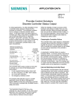
1
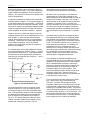
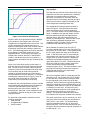
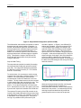
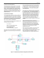
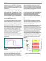
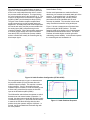
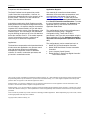
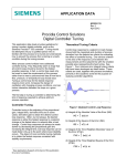
APPLICATION DATA AD353-127 Rev 2 April 2012 Procidia Control Solutions Dead Time Compensation This application data sheet describes dead time compensation methods. A configuration can be developed within a Siemens 353 controller 1 to perform the dead time compensation. Dead time is the period during which the process variable does not respond to a change in valve position; during that time, the process appears to be unresponsive, or “dead”. This delay can cause poor control performance. Where dead time is the dominant dynamic element in the control loop, some type of dead time compensation is required to improve control loop performance. In the purest sense, dead time results from a transport delay as shown in Figure 1. The composition of the effluent that is measured by the analyzer (AT) is controlled by manipulating the reagent valve. Since the analyzer is located some distance from the discharge of the mixing vessel, the effect of any change in the composition will take some time to reach the analyzer. In this case, the value of the dead time is the quotient of the distance the fluid must travel divided by the velocity at which it is traveling. Thus, other descriptive terms that are synonymous with dead time are distance-velocity lag, transport lag, and pure delay. Although dead time is present to some degree in nearly all process control loops, the dynamic behavior of most loops is dominated by one or more capacity lags in series with the dead time. Capacity refers to the ability of the process to store mass or energy. For the process shown in Figure 1, the larger the capacity of the vessel, the longer it will take for a change in reagent flow to affect the composition. Thus, other terms that are synonymous with capacity lag are first-order lag and exponential lag. Reagent Figure 2 shows the response of a dead time element in series with a single capacity lag. 100% Influent 100% M θ AC 0 T Input 0 Dead Time 100% AT Effluent Dead Time = Distance Velocity θ 0 See Applications Support at the back of this publication for a list of controllers. T Dead Time + Lag Dead Time Capacity Lag θ τ Figure 1 Process with Dead Time 1 τ Figure 2 Dead Time + Capacity Lag T AD353-127 Note that the dead time does not alter the shape of the input signal in any way. It only shifts (delays) the signal in time before passing it on the next dynamic element. The symbol θ is often used to represent the value of the dead time. dimensionless number based on changes in normalized process variable and valve signals. Whether or not it is necessary to use dead time compensation in a control loop depends on the relative magnitude of the effective dead time and the effective time constant of the loop. One minute of dead time may not be significant if the process time constant is 10 minutes of more. However, one minute of dead time can cause severe problems in a loop with a one minute time constant. Dead time compensation should be considered whenever the ratio of dead time to time constant (θ/ τ ) exceeds 0.5. A capacity lag exhibits the characteristic exponential response shown in Figure 2. The response begins at a rate determined by the time constant ( τ ) and slows down continuously as the response proceeds. At the initial rate of change, the exponential response would follow the tangent line shown in Figure 2 and would reach completion in one time constant ( τ minutes). However, due to the continuous change in rate, the response reaches 63.2% of the total response in one time constant. In each successive time constant interval, the response moves 63.2% of the distance remaining. Theoretically, the exponential response never reaches completion, but for all practical purposes, the exponential response is complete in about 4 time constants. A process control loop that is dominated by dead time responds slowly and is only marginally stable. Conventional control strategies use Proportional + Integral (PI) or Integral-Only (I) controllers on these loops. The Derivative mode is not very effective in loops dominated by dead time. For stability, the proportional gain of the controller may be set relatively low (<1) and the integral time may be set relatively long (several minutes). With these settings, the controller will be slow to respond to a load change, and the control errors that result can be relatively large in magnitude and duration. For multiple lags in series with a dead time element, the process responds as shown in Figure 3. This is a typical process reaction curve. As an approximation, the response can be characterized by an effective dead time (θ), and effective time constant ( τ ), and a steady-state gain (Kp). A conventional PI controller has difficulty with dominant dead time due to the initial lack of process feedback to the proportional action of the controller. When a load disturbance causes a control error between the process variable and the setpoint, the proportional action of the controller provides an immediate change in the valve position. This proportional change might be all that is required to correct the control error. However, there is no immediate feedback of this fact to the controller due to the dead time of the process. 100% PV PV Kp = V PV θ τ V Valve 0 Dominant Dead Time θ τ > 0.5 Figure 4 shows the controller response to a dead time + lag process using a conventional PID controller. A setpoint (SP) change causes an immediate change in the controller output (CO) due to Proportional + Integral action, while the process variable (PV) responds some time later. The process used to simulate this response has a dead time (θ) of 0.2 minutes and a lag time ( τ ) of 0.08 minutes. The same process simulator will be used to illustrate all the examples in this document. A critically damped tuning response will be used for all examples. Figure 3 Process Reaction Curve The effective dead time can be caused by a pure dead time element, or it can be caused by one or more capacity lags in series with a dominant dead time. The approximate dead time and time constant are determined by drawing a tangent through the point of inflection in the reaction curve shown in Figure 3. The steady state gain is the ratio of the change in process variable to the change in valve position that caused the response. This is a 2 AD353-127 Step and Wait The step and wait controller mimics the actions of an experienced control room operator who is manually controlling a process dominated by dead time. Whenever it is necessary to move the valve, the operator makes a valve change (the step) and then waits for the process to respond completely to that valve change before making another step. The configuration of a step and wait controller is shown in Figure 5. PID controller function block output is interrupted by a Track and Hold block (TH1). This block holds the valve position between steps. In addition to the controller output, the PID block provides a signal (AE) that represents the absolute value of the control error between the process (P) and setpoint (S). Whenever the control error exceeds an adjustable threshold value, comparator (CMP1) provides a logic signal that initiates the step and wait timing cycle. Figure 4 Conventional PID Response While the effect of the proportional action is delayed by the dead time, the integral mode “sees” and integrates the full magnitude of the control error. This tends to exaggerate the integral action since it appears to the integral mode of the controller that the proportional mode has done nothing to reduce the error. This initial exaggeration can only be cancelled by integrating a comparable control error in the opposite direction. To minimize these swings, the integral action must be “detuned” or slowed down. However, this allows control errors to persist for a longer period of time before they are corrected by the controller. When enabled, the repeat cycle timer (RCT1) provides a periodic pulse to the track command (TC) input of the TH1 function block. In the tracking mode, the TH1 block passes the output of the PID to the Valve. In the hold mode, the TH1 block holds the valve position until it is time for the next step. The integral action of the PID controller is disabled by holding the reset feedback signal (input F) at the value stored by the TH1 block. This also biases the PID block so that its output is always equal to the current valve position plus the proportional component (gain x error). This ensures that the valve step that occurs during the track pulse is equal in magnitude and direction to the proportional component of the controller. Some of the most critical quality control loops in a plant are often the ones that are dominated by dead time. Therefore, there is usually a large economic incentive to improve the performance of these loops. The most direct way to avoid control problems caused by excessive dead time is to take steps to eliminate dead time wherever practical. For example, relocating the analyzer shown in Figure 1 closer to the mixing vessel could result in a significant improvement in the performance of the loop. When the comparator (CMP1) initiates the step and wait timing cycle, the on-delay timer (DYT1) delays the first step in the sequence long enough to allow the full magnitude of the control error to develop. Otherwise, the first step will be triggered prematurely and will be based only on the threshold setting of the comparator, rather than the full size of the upset that is causing the control error. As long as the error persists, subsequent steps will occur periodically as determined be the repeat cycle timer (RCT1) settings. The delay timer setting should be about four times the first order time constant of the process. If dead time cannot be significantly reduced, consider using feedforward and cascade control strategies to correct for load disturbances before they can adversely affect the critical control variable. By decreasing the “work load” on the troublesome loop, it is possible to minimize the impact of poor control loop performance. For dead time compensation consider one of the following techniques; • Step and Wait • Complementary Feedback • Smith Predictor The repeat cycle timer is set for a minimum “on” time (0.01 min) which is converted by the one shot timer (OST1) to a 0.1 sec. pulse. The period between pulses is essentially equal to the “off” time of the repeat cycle timer. The “off” time should be set long enough to allow the process to respond completely to the last step (θ + 4 τ ). 3 AD353-127 Figure 5 Step and Wait Configuration (CF353-127SW) The A/M transfer switch allows the operator to switch between auto and manual modes of operation. In manual, the MS status signal from the A/M function block provides a track command signal to the track and hold (TH1) via the OR logic block (OR1). In addition, the AS status signal from the A/M function block provides a track command signal to controller (PID). This aligns the output of the PID and TH1 blocks with the valve position set by the operator using the A/M block. around the setpoint. In Figure 6, two different PG settings are illustrated. In the first response (PG of 1.0) to a setpoint (SP) change, the change in the controller output (CO) caused the process variable (PV) to overshoot the setpoint. Two cycles of the repeat cycle timer were needed to bring the process to setpoint. In the second response (PG = 0.85) to a setpoint change, the change in the valve caused the process to slightly undershoot the setpoint and a second small correction was required. This illustrates the affect of the PG settings on the tuning of the step and wait controller. Step and Wait Tuning The step and wait controller is tuned by first setting the timers and then finding the optimum controller gain (PG). The integral and derivative parameters are both set to minimum values (TI = 0.01 minutes and TD = 0.0 minutes). To set the timers, it is necessary to conduct a step response test to generate a process reaction curve. However, it is not necessary to obtain precise measurements of either the dead time or the time constant. The key measurement is the time required to reach steady state after introducing the step. This is the “off” time setting of the repeat cycle timer (RCT1). To set the on-delay time of function block DYT1, decrease the time set in the repeat cycle timer by an amount equal to the estimate of the dead time. Figure 6 Step and Wait Controller Response Although the step and wait controller can bring the process to setpoint quickly compared to a conventional PID controller, it does not eliminate the dead time of the process. As mentioned previously, reducing the process dead time will provide the greatest improvement on control of the process. The optimum PG setting of the PID controller is the inverse of the steady-state gain of the process (1/Kp). If the PG setting is correct, it is possible to correct for a disturbance in one complete cycle. If the gain is too high it is possible that the process will cycle 4 AD353-127 Comparison with Other Methods The reset feedback signal to the PI function block is actually the input to a first-order lag that is built into the PID algorithm. The time constant for this lag is the integral time (TI). The output of the lag is the reset component R. The step and wait controller provides a very robust method of dead time compensation. It is relatively easy to identify the parameters required to set the timers. Once the timers are set, controller tuning is reduced to a “one knob” (PG) tuning problem. The step and wait controller provides the best solution in applications where the process response is almost entirely dead time. Note that the reset feedback signal is generated by the controller output. It is this positive feedback from the controller output to the reset component that generates integral action at a rate determined by the value of the integral time constant. By inserting a dead time element in the reset feedback path, the response of the reset component can be tuned to match the response of the process variable. This results in positive reset feedback that opposes (complements) the negative feedback of the process variable. Complementary Feedback The complementary feedback controller modifies the reset feedback signal to a conventional PI controller. A dead time element is inserted in the reset feedback path to delay the integral action while the affect of the proportional action is delayed by the process dead time. Figure 7 shows a configuration. With conventional PI control, a control error generates an immediate change in valve position (G x E) from proportional action. However, this proportional component returns to zero when the control error returns to zero. Only integral action changes the controller output from one steady state operating level to another without incurring a sustained control error. The conventional PI controller output is based on the following steady state equation: O=GxE+R where: O is the controller output G is the proportional gain E is the control error R is the reset (integral) component With complementary feedback, the response of the reset component matches the response of the process variable to the proportional change in output. Then, as the control error decays, the reset component adds to the controller output about the Note: refer to the 353 User Manual for more detailed information of the actual working of the PID function block Figure 7 Complementary Feedback Configuration (CF353-127CF) 5 AD353-127 same amount that the proportional component subtracts from the controller output. This holds the valve near the initial change in position without any additional control error or overshoot due to excessive integral action. showed a slightly over-damped response while the second shows a slight overshoot to the setpoint change. Although the ideal response is limited, the complementary feedback controller provides greatly improved response over the standard PID controller. The configuration of a complementary feedback controller is shown in Figure 7. This is a conventional single loop configuration with a dead time block DTM1 inserted in the reset feedback path. The A/M block furnishes a logic signal to the DTM1 block for it to bypass the dead time function whenever the A/M block is in the manual position. This allows the PID controller to track the valve position in manual without the dead time delay. Comparison with Other Methods Complementary Feedback Tuning Smith Predictor The complementary feedback controller is tuned by setting the dead time block equal to the process dead time (θ), the integral time constant to match the process time constant ( τ ), and then by finding the optimum controller gain (PG). The derivative mode is disabled by setting the derivative time to zero. Like the step and wait controller, it is necessary to conduct a step response test to generate a process reaction curve. In this case, however, an accurate estimate of the process dead time and time constant is more important. A reasonable starting point for the PG setting is one-half the inverse of the steady state gain of the process ( 0.5/Kp). The gain can then be increased to obtain the desired response. The Smith Predictor is a dead time compensation strategy that is based on an internal process model. The process model consists of a dead time, firstorder lag, and steady state gain. The complementary feedback controller depends on a more accurate estimate of the process parameters than the step and wait controller. Therefore, it is perhaps less robust than the step and wait. However, the configuration of the complementary feedback controller is much simpler than either of the other alternatives, and it is still relatively easy to tune. Figure 9 shows a block diagram of the Smith Predictor. The controller output provides the input to the process model as well as the actual process. Note that the process model had two separate model components: one with dead time included and one without dead time. If there is a good match between the dynamics of the model and the process, the output of the model with dead time will cancel the output of the process. The process variable signal that remains for the controller will be the output of the model without dead time. This has the effect of mathematically eliminating the dead time from the control loop. The controller can then be tuned, and the loop should perform as if the process had no dead time. Figure 8 shows the response of the complementary feedback controller on a dead time + lag process. This is the same simulated process used throughout this publication. SP Error + Controller Ouput _ + _ Process Model with Dead Time + Figure 8 Complementary Feedback Controller Response PV Two step tests were performed to illustrate the affect of controller gain changes. The useful gain has a very narrow range of adjustment. In the first step test the controller gain (PG) was set for 0.95 and the Integral Time (TI) for 0.08. In the second test the controller gain was increased to 1.05. The first test Process Model without Dead Time Process Valve Figure 9 Smith Predictor Block Diagram 6 AD353-127 Smith Predictor Tuning The configuration for a Smith Predictor is shown in Figure 10. A conventional PID controller (derivative action is not used) manipulates the valve to control the process variable at setpoint. The signal driving the valve is also the input to the lag block (LL1). The output of the lag block is connected to the deviation amplifier (DAM1) and the dead time block (DTM1). The gain of the deviation amplifier amplifies both model components to provide a steady state gain adjustment. At steady state, both model components will cancel each other, and the process variable from the analog input (AIN1) will pass through to the controller unaltered. During the transient response to a controller output change, the output of the dead time table (DTM1) will cancel the process variable, and the controller will actually be controlling the lag block output signal. Set the model parameters to match the effective dead time, time constant, and steady state gain of the process. To accomplish this, it is necessary to conduct a step response test, and the process parameters should be identified with as much accuracy as possible. The controller is then tuned using conventional controller tuning techniques. Figure 11 shows a response test of the dead time process using the Smith Predictor. The initial response used tuning similar to the Complementary Feedback and showed similar results. The Smith Predictor will enable higher controller gain while maintaining process stability. In the second response the controller gain was increased to 8. Figure 10 Smith Predictor Configuration (CF353-127SP) The configuration shown in Figure 10 assumes that the process variable (PV) will increase when the controller output increases. This requires a reverse acting controller. If the PV decreases when the controller output increases, it will be necessary to use a direct acting controller and reverse the A and B input to the deviation amplifier (DAM1). The A/M transfer switch allows the operator to switch between auto and manual modes of operation. In manual, the status output signal (AS) provides a track command to the PID, LL1, and DTM1 function blocks. In manual, the PID block will align with the valve position set by the operator using the A.M block. In manual, the lag and dead time blocks will align with the valve position. Figure 11 Smith Predictor Response 7 AD353-127 Comparison with Other Methods Application Support The Smith Predictor has the potential to provide “perfect” dead time compensation. However, its performance depends entirely on the accuracy of the process model. Therefore, it is less robust than either of the alternatives discussed. User manuals for controllers and transmitters, addresses of Siemens sales representatives, and more application data sheets can be found at www.usa.siemens.com/ia. To reach the process controller page, click Process Instrumentation and then Process Controllers and Recorders. To select the type of assistance desired, click Support (in the right-hand column). See AD353-138 for a list of Application Data sheets. It should be noted that the Smith Predictor provides better performance for setpoint changes than it does for load changes. On setpoint changes, the transient response of the internal model is in sync with that of the process since the source of the disturbance is the controller output. On load changes, the disturbance may be affecting the process up to one full dead time before the controller “sees” it. If the model response is out of sync with the process, it cannot do as effective a job of dead time compensation. The configuration(s) shown in this publication were created in Siemens i|config™ Graphical Configuration Utility. Those with CF353 in parenthesis in the Figure title are available using the above navigation, then click Software Downloads > 353 Dead Time Compensation (Reference AD353127). Applications The configuration(s) can be created and run in a: • Model 353 Process Automation Controller • Model 353R Rack Mount Process Automation Controller* • i|pac™ Internet Control System* • Model 352Plus™ Single-Loop Digital Controller* * Discontinued model The dead time compensation techniques described in this document are applicable to any process control loop with dominant dead time characteristics. Examples are composition control of distillation columns, O2 control in combustion processes, and pH control in neutralization tanks. i|pac, i|config, Procidia, and 352Plus are trademarks of Siemens Industry, Inc. Other trademarks are the property of their respective owners. All product designations may be trademarks or product names of Siemens Industry, Inc. or other supplier companies whose use by third parties for their own purposes could violate the rights of the owners. Siemens Industry, Inc. assumes no liability for errors or omissions in this document or for the application and use of information in this document. The information herein is subject to change without notice. Siemens Industry, Inc. is not responsible for changes to product functionality after the publication of this document. Customers are urged to consult with a Siemens Industry, Inc. sales representative to confirm the applicability of the information in this document to the product they purchased. Control circuits are provided only to assist customers in developing individual applications. Before implementing any control circuit, it should be thoroughly tested under all process conditions. Copyright © 2012, Siemens Industry, Inc. 8