Download Display - Siemens

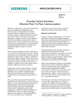
APPLICATION DATA
AD353-119
Rev 2
April 2012
Procidia Control Solutions
Digital Controller Tuning
This application data sheet provides guidelines for
tuning a modern digital controller, such as the
Siemens Procidia™ 353 controller 1 . Tuning should
be attempted only by a qualified person who is
familiar with the process to be tuned and understands
how to prevent the process from entering an unsafe
condition during the tuning process.
Many process control articles have addressed
controller tuning. They frequently seem to imply that
all control loops should be tuned for the fastest
possible response. In fact, a control loop need only
be tuned to meet the requirements of the process
rather than to meet a preconceived idea of how fast a
flow, pressure, or temperature loop should react.
Tuning a control loop for the fastest response
requires more work, increases the danger of
oscillation with changing process conditions, and can
induce interaction between the loops on a given
process.
Theoretical Tuning Criteria
Control loop response to a setpoint or load change
shows both the magnitude and duration of process
deviation from the setpoint as criteria for evaluating
the effect of controller tuning. One obvious criterion
is the area of the response curve between the
measurement and the setpoint line with the smallest
possible area representing the best tuning. See
Figure 1. Four minimum error integral tuning criteria
that have been developed are listed below. These
criteria are used, together with process simulations,
primarily in the academic world for the purpose of
studying controller algorithms.
The first step in tuning a controller is determining the
kind of response required to achieve optimum
process operation.
Controller Tuning
Figure 1 Idealized Control Loop Response
Controller tuning is the adjusting of the proportional
gain, integral time, derivative time and in some
cases, derivative gain to obtain the desired control
loop response. Often, but not always, the desired
response is either the fastest response to a setpoint
change or the fastest return to setpoint after a load
change. Control loop response can always be made
slower by decreasing the proportional gain and
increasing the integral time, but loop response can be
made faster only up to the point where loop instability
occurs. The object of most controller tuning methods
is to obtain the fastest response consistent with
stability requirements.
a) Integral of the Absolute Value of the Error (IAE)
IAE =
∫
b) Integral of the Square of the Error (ISE)
ISE =
∫
See Applications Support at the back of this publication
for a list of controllers.
e2(t) dt
c) Integral of the Time Weighted Absolutes Value of
the Error (ITAE)
ITAE =
∫
t|e(t)| dt
d) Integral of the Time Weighted Square of the Error
(ITSE)
ITSE =
1
|e(t)| dt
∫
te2(t) dt
AD353-119
The ISE tuning criterion [see b) above] puts more
weight on large errors as compared with the IAE [see
a) above]. The ITAE and ITSE are similar except
they include a weight for elapsed time. Because of
the uncertainties in process control loops, it is seldom
possible or practical to meet even one of these
criteria precisely. However, the ideas presented are
useful in evaluating the suitability of a control
response for a particular process.
danger of continuous oscillation under changed
process conditions.
With a proportional only controller, quarter decay
response comes close to meeting minimum area
criterion. Therefore, it is only necessary to adjust the
proportional gain to obtain a quarter decay response
to be assured that the control response to an upset
will be about as fast as practical. When integral and
derivative modes are added, it is possible to obtain
quarter decay responses with longer and shorter
periods; quarter decay does not assure minimum
area. It is necessary to find the right combination of
controller adjustments to obtain optimum response.
Fortunately tuning for an area criterion usually results
in a response similar to quarter decay, so the desired
degree of stability can be maintained.
Loop Stability
The effectiveness of controller tuning is also judged
by the degree of stability of the loop response. For
oscillatory responses, the degree of stability is
indicated by the decay ratio (i.e. the ratio of
successive peaks of the response). See Figure 2.
A critical or even a highly damped response is
employed on control loops where oscillation is
undesirable, such as level control used for flow
smoothing. Tuning for critical damping is not covered
here.
Ziegler-Nichols Tuning Methods
The following tuning methods were developed
through considerable experimentation and have
become industry recognized methods for calculating
controller adjustments from measurements made on
the process. They are intended to yield quarter
decay and reasonably fast response and are based
on experience with typical processes. No specific
tuning criterion is used.
Figure 2 Loop Response, 1/4 Decay Ratio
For non-oscillatory responses, the degree of stability
can be expressed as the damping factor. A damping
factor of 1 represents the fastest possible response
without overshoot and is called critical damping. See
Figure 3.
A. Ziegler-Nichols Closed Loop Method
1. Bring the process to the desired setpoint on
manual control.
2. Eliminate integral and derivative action by
adjustment – maximum integral and
minimum derivative times.
3. Adjust the proportional gain to the lowest
setting and switch the control system to
automatic.
4. Simulate a process upset by making a small
momentary change in the setpoint. Look for
a sustained cycle in the measurement on the
controller output. If no cycle results, increase
the proportional gain and try again. Repeat
until a sustained cycle of continuous
amplitude appears.
5. Note the lowest proportional gain at which
cycling is sustained. This is the ultimate
proportional gain PGu.
6. Time one complete process cycle, from
positive peak to positive peak, in minutes.
This is the ultimate period Tu.
Figure 3 Loop Response, Critical Damping
Quarter decay response is often used in tuning for
process control simply because it represents a useful
compromise between fast response and stability, and
it includes a safety factor to reduce the possibility of
continuous oscillation on a change in loop
characteristics. A higher decay ratio (a ratio of 1
indicates continuous oscillation) would produce a
more sustained oscillation and would increase the
2
AD353-119
7. Determine controller adjustments from the
table below.
be necessary to readjust the proportional gain,
integral, or derivative to obtain the desired result.
However, Ziegler-Nichols usually results in a
response close to quarter decay so only minor
readjustments should be necessary.
Controller Tuning Constants
TUNING
TYPE OF CONTROLLER
PARAMETER
P
PI
PD*
PID
Proportional Gain
0.5
0.45
0.71
0.6
(PG)
PGu
PGu
PGu
PGu
Integral
--0.83
--0.5
(TI – minutes)
Tu
Tu
Derivative
----0.15
0.125
Tu
Tu
(TD – minutes)
* Not from the original Ziegler-Nichols Paper
It is often found that PGu and Tu will change if tuning
is repeated at a different setpoint or under different
load conditions. This can occur as a result of nonlinearity in valves or transmitters or changing
throughput in the process. Consequently, optimum
control response can be attained only with a
particular set of conditions and can be expected to
change – to become slower or more oscillatory – as
conditions change. This indicates the need for a
safety factor in the controller tuning or the use of
adaptive gain control.
B. Ziegler-Nichols Open Loop Method
1. Bring the process to the desired setpoint on
manual control.
2. Change the valve position a small amount ∆V
(%). The change should be large enough to
produce a measurable response in the
process but not large enough to drive the
process beyond the normal operating range.
A 5% valve change is a good starting point.
3. Measure C and L (see Figure 4) on the
process response curve.
4. Calculate:
PGu =
2( ΔV )
ΔC
Low Gain Tuning for Flow Control
Although Ziegler-Nichols tuning may not work
particularly well for flow control, this is not a serious
problem. Flow control response, particularly liquid
flow, is usually fast enough so that tuning by trial and
error requires little time. One method is to set the
proportional gain to a low setting (usually 0.2) and
then adjust the integral time to obtain quarter decay
or other desired response. Results should be close
to any faster response obtained with a different
combination of proportional gain and integral, and
should be more than fast enough for most process
requirements as satisfactory results are usually
obtained with one setting.
Tu = 4 L
5. Determine the controller settings from the
previous table.
Derivative Gain
For a step change in the process variable, the
derivative mode adds an impulse component to
the controller output. The magnitude of the
impulse is related to the derivative gain. The
rate at which the impulse decays is related to
the ratio of the derivative time and the derivative
gain. The factory configured value for the
derivative gain is 10 and does not normally
need to be changed.
The derivative mode is not recommended for
“fast” control loops with “noisy” process signals (e.g.
flow control). The derivative gain amplifies the noise
component causing excessive activity in the
controller output signal. However, it may be possible
to use derivative on some “noisy” loops (e.g.
temperature or level control) by reducing the
derivative gain. This provides a “weak” derivative
response that retains some of the benefit of the
derivative mode while reducing the detrimental
effects of the noise amplification.
Figure 4 Process Response Curve
C. Limitations
Tuning constants listed in the table are based on
experience with typical processes. A number of
common processes may show non-typical responses,
including liquid level and liquid flow control, but the
tuning constants usually work fairly well. On any
process the initial results of Ziegler-Nichols tuning
may not produce quarter decay response and it may
3
AD353-119
In essence, the derivative gain provides a noise filter
adjustment for the derivative mode. To increase the
filter time constant, decrease the derivative gain. To
achieve less filtering, increase the derivative gain
the Siemens Internet site. See the navigation
suggestion below.
Application Support
Automatic Tuning Controller
User manuals for controllers and transmitters,
addresses of Siemens sales representatives, and
more application data sheets can be found at
www.usa.siemens.com/ia. To reach the process
controller page, click Process Instrumentation and
then Process Controllers and Recorders. To select
the type of assistance desired, click Support (in the
right-hand column). See AD353-138 for a list of
Application Data sheets.
Many modern digital controllers have built-in
automatic tuning capability. A number of methods for
determining the process dynamics have been used.
These include parameter estimation, recursive
computation, and describing function analysis
(reference ISA - Automatic Tuning of PID
Controllers). The Siemens 353 controller includes
automatic tuning based on describing function
analysis. This method temporarily substitutes an
ON/OFF control function, which includes hysteresis,
for the PID function. The ON/OFF cycle period along
with the gain of the measurement/valve are used with
the describing function to determine the ultimate gain
and ultimate period of the process. The controller
uses these values to determine recommended P, I,
and D settings. More information about the tuning
method can be found in the User Manual for a
Siemens 353 controller, e.g. UM353-1B, available on
The tuning concepts in this publication can be applied to a:
•
•
•
•
Model 353 Process Automation Controller
Model 353R Rack Mount Process Automation
Controller*
i|pac™ Internet Control System*
Model 352Plus™ Single-Loop Digital Controller*
* Discontinued model
i|pac, i|config, and 352Plus are trademarks of Siemens Industry, Inc. Other trademarks are the property of their respective owners. All
product designations may be trademarks or product names of Siemens Industry, Inc. or other supplier companies whose use by third parties
for their own purposes could violate the rights of the owners.
Siemens Industry, Inc. assumes no liability for errors or omissions in this document or for the application and use of information in this
document. The information herein is subject to change without notice.
Siemens Industry, Inc. is not responsible for changes to product functionality after the publication of this document. Customers are urged to
consult with a Siemens Industry, Inc. sales representative to confirm the applicability of the information in this document to the product they
purchased.
Copyright © 2012, Siemens Industry, Inc.
4