Download User manual

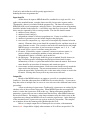
more than two traits, parameter estimates are not shown in the summary statistics table
(the number of parameters grows quickly with many traits). See Hohenlohe and Arnold
(2008) for further details on how to interpret the results.
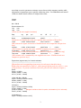
39 taxa
2 traits
Ne = 500.00
Direct estimate of G:
7.53
1.98
1.98
7.98
[These are the user-supplied estimates]
Step
sig
eps
phi
lnL
LR
df
p
---------------------------------------------------------------------------------------------------------Direct
15.50500.6288 0.8425
-408.37 -
[Parameters and likelihood for the user-supplied direct estimates of G and Ne.]
1.Size
0.3075 0.6288 0.8425
-293.71 229.33 1
0.0000
[ML estimate for sigma, and results of likelihood ratio test comparison with previous
step.]
2.Shape
0.3381 0.7925 0.8425
-290.57 6.28
1
0.0122
[ML estimate for epsilon and sigma, with LRT comparison to previous step.]
3.Orientation
0.3380 0.8705 0.5130
-283.20 14.74
1
0.0001
[ML estimate for all G-matrix parameters, with LRT comparison to previous step.]
Test vector
0.3380 0.8688 0.4636
-283.42 0.44
1
0.5072
[ML estimate of G, constrained by user-supplied test vector. Likelihood ratio test
compares to previous step.]
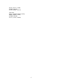
Eigenvalues (eigenvectors) for G-matrix estimates:
-------------------------------------------------------------------
[Eigenvalues and corresponding eigenvectors for each step in the table above.
Eigenvalues are normalized to sum to 1, with sigma giving the total size of G (i.e., sum
of eigenvalues). 95 percent confidence limits are given for each estimate of sigma.]
Direct:
Sigma = 15.5050
0.6288 (0.6656 , 0.7463)
0.3712 (0.7463 , -0.6656)
1.Size (with Ne = 500.00):
Sigma = 0.3075 [0.2282 to 0.4283]
0.6288 (0.6656 , 0.7463)
0.3712 (0.7463 , -0.6656)
2.Shape(1):
Sigma = 0.3381 [0.2509 to 0.4708]
0.7925 (0.6656 , 0.7463)
[0.6767 to 0.8618]
[Marginal confidence limits for epsilon; calculated only for 2-trait case]
0.2075 (0.7463 , -0.6656)
3.Orientation(1):
Sigma = 0.3380 [0.2509 to 0.4707]
3