Download ExaFMM - User`s Manual

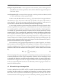
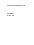
ExaFMM
Fast multipole method software aiming for exascale systems
User's Manual
Rio Yokota, L. A. Barba
November 2011 --- Revision 1
ii
ExaFMM
Revision History
Name
Date
Notes
Rio Yokota, L A Barba
10/21/2011
Original Document
Rio Yokota
10/25/2011
Revision 0.1
Rio Yokota
10/30/2011
Revision 0.2
ii
iii
ExaFMM User's Manual
Contents
1
Introduction
1
2
Download & Install
2.1 Download . . . . . . . . . . . . . . . . . . . . . . . . . . . . . . . . . . . . .
2.2 Install . . . . . . . . . . . . . . . . . . . . . . . . . . . . . . . . . . . . . . . .
1
1
1
3
Test suite
3.1 Unit tests . . . . . . . . . . . . . . . . . . . . . . . . . . . . . . . . . . . . . .
3.2 Regression tests . . . . . . . . . . . . . . . . . . . . . . . . . . . . . . . . . .
1
1
4
4
Algorithm description
4.1 Hierarchical space decomposition . . . . . . . . . . . . . . . . . . . . . . . .
4
5
5
Using ExaFMM in application programs
6
iii
1
ExaFMM User's Manual
1
Introduction
This manual describes ExaFMM, a free implementation of FMM in C++. It is available to
all users, including commercial, and uses the very permissive MIT license, allowing it to
be included in commerical codes.
The first release of ExaFMM was in November 2011. It is freely downloadable from
https://bitbucket.org/exafmm/exafmm, and we welcome correspondence with potential users or those who wish to extend it for specific purposes.
2
2.1
Download & Install
Download
If you have mercurial, simply do
hg clone https://[email protected]/exafmm/exafmm
if not, you may download the source from https://bitbucket.org/exafmm/exafmm/
overview. There is a link on the right that says ``get source".
2.2
Install
To use ExaFMM as a black box library do
cd exafmm
./configure
make lib
and set your library path to exafmm/wrapper, and add ``-lexafmm" to your library flags.
An MPI C++ compiler is required. If you want to run without MPI, open exafmm/Makefile
and change the variable CXX from mpicxx to g++. ExaFMM is designed so that the parallel
portion of the code is an extension of the serial portion of the code using class inheritance.
Therefore, all the serial parts of the code function with or without MPI, and there is no
need for a separate serial version.
The minimum installation of ExaFMM does not depend on any external libraries.
However, It does provide visualization routines that uses VTK (downloadable form http:
//www.vtk.org/VTK/resources/software.html) if the user chooses to use them, but the
FMM itself will function without VTK.
3
3.1
Test suite
Unit tests
All unit tests can be found in the directory unit test. The Makefile in this directory
contains the commands to run all the unit tests. For a very quick demonstration of an
1
2
ExaFMM
N -body calculation for N = 10, 000 bodies do:
cd unit_test
make serialrun
The result will be indicated by the output text. If you encounter any errors, please
send the full output text to [email protected].
Here is the full list of unit tests, and a short description of what they do.
index: Assigns Morton index to 107 bodies, and sorts the bodies according to the index.
If VTK is available, it will plot the group of bodies according to the index, with a
toggle bar that controls the group to be shown.
topdown: Constructs a tree structure top-down for 107 bodies. If VTK is available, it will plot
the group of bodies according to the leaf index, with a toggle bar that controls the
group to be shown.
bottomup: Same as topdown, except the tree construction is bottom-up.
kernel: Checks the convergence of kernels by doing P2M, M2M, M2L, L2L, L2P, and M2P
translations for a single pair of particles. The distance between the particles and the
cells that contain them is varied and the difference between a direct summation is
monitored. The default is the Laplace kernel but changing D.kernelName on line 14
allows you to check different kernels, as is the case with many other unit tests.
serialrun: Compares serial FMM with direct summation for 104 bodies.
unsort: Same as serialrun except it sorts back the bodies to their initial order. (FMM reorders
the bodies according to the Morton index).
Nserial: Same as serial run except it varies the number of bodies from 104 to 107 and checks
the O(N ) scaling.
direct gpu: Compares the serial direct summation on a GPU and CPU.
mpi: Prints the hostname, rank, and size of all MPI processes in order.
check gpus: Compares the parallel direct summation on many GPUs and CPUs. Prints the MPI
rank, GPU device ID, and Error between the CPU and GPU for every MPI process.
shift: Verification of communication routine ``shiftBodies" for sending bodies to the next
process in round-robin fashion. This allows the source bodies to be shifted to the
next process so that an all-pairs interaction can be calculated on distributed memory systems without increasing storage requirements. If VTK is available, the same
``shiftBodies" routine will be used to plot bodies on all processes without storing
all of them in one process. The toggle bar can be used to show bodies on different
processes.
2
3
ExaFMM User's Manual
nth element: Verification of parallel nth element routine. The nth element finds the nth element
of a sorted vector without actually sorting the vector. It is an efficient method for
finding the median. The parallel nth element finds the global nth element without
performing an actual parallel sort. If VTK is available, it will plot the bodies on both
sides of the nth element and toggles between the two. Only the bodies on MPI rank
0 will be plotted.
bisection: Verification of recursive multi-section partitioning. If VTK is available, it will plot
each of the partitioned domains (one per process), and toggle between all domains.
It will partition the domain into equal number of bodies for any number of processes.
let: Verification of local essential tree (LET). Partitions the domain using multi-section,
performs a parallel tree construction, and communicates the LET. If VTK is available, it will plot the bodies and cells on each process, and toggle between the bodies
and cells on every process.
parallelrun: Parallel version of serialrun. Compares parallel FMM with direct summation for
104 bodies. If VTK is available it will plot the same thing as let, but this time for
the actual bodies and cells that were used in the FMM calculation.
unpartition: Same as parallelrun, except it (un)partitions the bodies back to their original distribution among processes, and (un)sorts them back to their original order within
each process at the end.
ijparallelrun: Same as unpartition, except it has different distribution for target bodies and source
bodies.
Nparallel: Parallel version of Nserial. Varies the number of bodies from 104 to 107 and checks
the O(N ) scaling of the parallel FMM.
skip tree: Verification of tree construction skipping. Same as parallelrun except it does two
FMM calculations, and in the second one it skips the tree construction and uses the
tree structure from the first FMM.
overlap comm: Verification of communication overlapping. Same as skip tree, except it overlaps
the communication with the computation of the local tree using OpenMP.
vtk: Verification of VTK plotter. Plots two groups of bodies, with a bar that toggles between them.
cuprintf: Verification of cuprintf --a printf routine that prints from inside kernels that works
even on old GPUs.
3
4
3.2
ExaFMM
Regression tests
There are no regression tests at the moment.
4
Algorithm description
The fast multipole method (FMM) is an algorithm for accelerating computations of the
form:
f (yj ) =
N
∑
ci K(yj , xi )
(1)
i=1
Such a computation may represent a field value evaluated at point yj , where the field
is generated by the influence of sources located at the set of centers {xi }. The sources are
often associated with particle-type objects, such as stellar masses, or charged particles.
The evaluation of the field at the centers themselves, therefore, represents the well-known
N -body problem. In summary: {yj } is a set of evaluation points, {xi } is a set of source
points with weights given by ci , and K(y, x) is the kernel that governs the interactions
between evaluation and source particles. The objective is to obtain the field f at all the
evaluation points, which requires in principle O(N 2 ) operations if both sets of points have
N elements. Fast algorithms aim at obtaining f approximately with a reduced operation
count, ideally O(N ).
The FMM works by approximating the influence of a cluster of particles by a single
collective representation, under the assumptions that the influence of particles becomes
weaker as the evaluation point is further away, i.e., the kernel K(y, x) decays as |x − y|
increases, and that the approximations are used to evaluate far distance interactions. To
accomplish this, the FMM hierarchically decomposes the computational domain and then
it represents the influence of sets of particles by a single approximate value. The hierarchical decomposition breaks up the domain at increasing levels of refinement, and for each
level it identifies a near and far sub-domain. By using the hierarchical decomposition, the
far field can be reconstructed as shown in Figure 1.
Using the computational domain decomposition, the sum in Equation (1) is decomposed as
f (yj ) =
N∑
near
Nf ar
cl K(yj , xl ) +
l=1
∑
ck K(yj , xk )
(2)
k=1
where the right-most sum of (2), representing the far field, is evaluated approximately
and efficiently.
We now need to introduce the following terminology with respect to the mathematical
tools used to agglomerate the influence of clusters of particles:
4
5
ExaFMM User's Manual
Multipole Expansion (ME): a series expansion truncated after p terms which represents
the influence of a cluster of particles, and is valid at distances large with respect to
the cluster radius.
Local Expansion (LE): a truncated series expansion, valid only inside a sub-domain, which
is used to efficiently evaluate a group of MEs.
In other words, the MEs and LEs are series (e.g, Taylor series) that converge in different
sub-domains of space. The center of the series for an ME is the center of the cluster of
source particles, and it only converges outside the cluster of particles. In the case of an
LE, the series is centered near an evaluation point and converges locally.
As an example, consider a particle interaction problem with decaying kernels, where
a cluster of particles far away from an evaluation point is `seen' at the evaluation point
as a `pseudo-particle', and thus its influence can be represented by a single expression.
For example, the gravitational potential of a galaxy far away can be expressed by a single
quantity locally. Thus, by using the ME representing a cluster, the influence of that cluster
can be rapidly evaluated at a point located far away ---as only the single influence of the
ME needs to be evaluated, instead of the multiple influences of all the particles in the
cluster. Moreover, for clusters of particles that are farther from the evaluation point, the
pseudo-particle representing that cluster can be larger. This idea, illustrated in Figure ??,
permits increased efficiency in the computation.
The introduction of an aggregated representation of a cluster of particles, via the multipole expansion, effectively permits a decoupling of the influence of the source particles
from the evaluation points. This is a key idea, resulting in the factorization of the computations of MEs that are centered at the same point, so that the kernel can be written
as,
p
∑
K(xi , yj ) =
am (xi )fm (yj )
(3)
m=0
This factorization allows pre-computation of terms that can be re-used many times, thus
increasing the efficiency of the overall computation. Similarly, the local expansion is used
to decouple the influence of an ME from the evaluation points. A group of MEs can be
factorized into a single LE so that one single evaluation can be used at multiple points
locally. By representing MEs as LEs one can efficiently evaluate a group of clusters in a
group of evaluation points.
4.1
Hierarchical space decomposition
In order to utilize the tools of MEs and LEs, a spatial decomposition scheme needs to be
provided. In other words, for a complete set of particles, we need to find the clusters
that will be used in conjunction with the MEs to approximate the far field, and the subdomains where the LEs are going to be used to efficiently evaluate groups of MEs. This
5
6
ExaFMM
root
level 1
leaf level
Figure 1: Tree structure associated to spatial decomposition.
spatial decomposition is accomplished by a hierarchical subdivision of space associated
to a tree structure (quadtree structure in two dimensions, or an octree structure in three
dimensions) to represent each subdivision. The nodes of the tree structure are used to
define the spatial decomposition, and different scales are obtained by looking at different
levels of the tree. A tree representation of the space decomposition allows us to express
the decomposition independently of the number of dimensions of the space. Consider
Figure ?? where a quadtree decomposition of the space is illustrated. The nodes of the
tree at any given level cover the whole domain. The relations between nodes of the tree,
represent spatial refinement. The domain covered by a parent box is further decomposed
into smaller sub-domains by its child nodes. Thus, in the FMM the tree structure is used
to hierarchically decompose the space and the hierarchical space decomposition is used to
represent the near-field and far-field domains. As an example, consider Figure ?? where
the near-field for the black colored box is represented by the light colored boxes, and the
far-field is composed by the dark colored boxes.
5
Using ExaFMM in application programs
Here we discuss at a high level, how to interact with ExaFMM.
6
7
ExaFMM User's Manual
root
level 1
M2L
M2M
M2L
L2L
leaf level
x
x
P2M
L2P
Figure 2: The sketch illustrates the upward sweep and the downward sweep stages on
the tree. Each stage has been further decomposed into the following substages: P2M-transformation of particles into MEs (particle-to-multipole); M2M--translation of MEs
(multipole-to-multipole); M2L--transformation of an ME into an LE (multipole-to-local);
L2L--translation of an LE (local-to-local); L2P--evaluation of a LEs at particle locations
(local-to-particle).
7