1
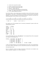
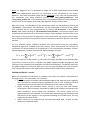
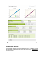
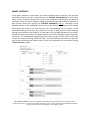
Since metal position is known, Smart Interface allows for a more efficient calculation of the anisotropy tensor, which can be estimated directly by using the following equations (see Bertini I et al., Progress in Magnetic Resonance Spectroscopy 40 : 249-‐273): 𝛿 !"# = 𝛿 !"# = 3𝑘 𝜒!! Where: 1 2𝑧 ! − 𝑥 ! − 𝑦 ! 𝑥! − 𝑦! 2𝑥𝑦 2𝑥𝑧 2𝑦𝑧 𝜒!! + 𝜒!! − 𝜒!! + 𝜒!" ! + 𝜒!" ! + 𝜒!" ! ! ! 4𝜋𝑟 2𝑟 2𝑟 ! 𝑟 𝑟 𝑟 ! ! ! ! ! 2𝑧!" − 𝑥!" − 𝑦!" 𝑥!" − 𝑦!" 2𝑥!" 𝑦!" 2𝑥!" 𝑧!" 2𝑦!" 𝑧!" + 𝜒!! − 𝜒!! + 𝜒!" + 𝜒!" + 𝜒!" ! ! ! ! ! 2𝑟!" 2𝑟!" 𝑟!" 𝑟!" 𝑟!" 𝑘 = − 𝑆!" 𝐵!! 𝛾! 𝛾! ℏ ! 4𝜋 15𝑘𝑇 2𝜋𝑟!" For which the first derivate can be easily obtained and included in a Gauss-‐Newton optimization approach. As for the Custom Interface, the contributions for each restraint are weighted by the specific weight present in the file, and by the global weight inserted in the dedicated textbox present in the interface. In case of joint estimation of the tensor using both PCSs and RDCs, the tensor related to RDCs is scaled by a factor equal to the model-‐free order parameter, which can be directly modified in the “General Parameters” field present in the interface. SMART INTERFACE -‐ Results After the calculation is complete, the results will be reported as explained in Custom Interface. In addiction to the tabs showing the data for each tensor, the “Tensor All” tab is generated reporting the superimposing correlation plots of the calculated tensors together with the global Q-‐factor (Fig. 5). Global Q-‐factor in calculated as a usual Q-‐factor on all the experimental data. Fig. 5: Smart Interface. It automatically generates a summary of all calculated tensors, including the plots showing the agreement between experimental and calculated data for the different tensors.