Download CytoViva Hyperspectral User Manual: 4.8 Features

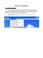
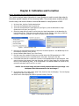
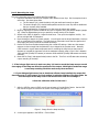
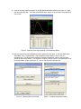
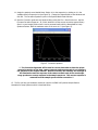
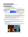
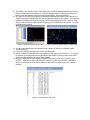
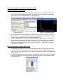
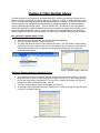
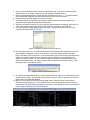
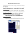
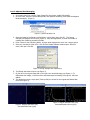
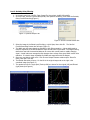
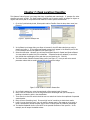
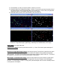
CytoViva Hyperspectral User Manual:
4.8 Features
IMPORTANT: PLEASE READ CAREFULLY
Limited Warranty
CytoViva warrants for a period of one (1) year from the date of purchase from CytoViva, Inc. or an authorized agent of CytoViva,
Inc. (the “Warranty Period”), that the unmodified CytoViva® adapter and/or Dual Mode Fluorescence Module (the “Equipment”)
when new, and subject to normal use and service, shall be free of defects in materials and workmanship and shall perform in
accordance with the manufacturer's specifications.
If any component of the Equipment does not function properly during the Warranty Period due to defects in material or
workmanship, CytoViva will, at its option, either repair or replace the component without charge, subject to the conditions and
limitations stated herein. Such repair service will include all labor as well as any necessary adjustments and/or replacement parts.
If replacement components are used in making repairs, these components may be remanufactured, or may contain remanufactured
materials. Repair or replacement without charge is CytoViva’s only obligation under this warranty. This warranty is NOT transferable
from the original purchaser of the Equipment.
Limitations
Other components of the product package, specifically including, but are not limited to, the light source(s), light source power
transformer(s) and cord(s), liquid light guide(s), optical filters, spectrophotometer, camera(s), software, microscope part(s), and
motorized stage are warranted based on the individual original manufacturer's warranties and policies. There is no warranty
whatsoever on the contrast filters, bulbs or the coil (on the motorized stage) purchased as part of the Equipment.
This warranty does not cover circumstances beyond CytoViva’s control, breakage, or a malfunction that has resulted from improper
or unreasonable use or maintenance, accident, tampering, misuse, neglect, improper installation, modification, improper
maintenance or service, cleaning procedures, shipping or repacking of Equipment, or service or parts to correct problems where
such service or parts are performed or provided by anyone other than CytoViva or an authorized agent of CytoViva; service required
as the result of unauthorized modifications or service misuse or abuse; failure to follow CytoViva’s operating, maintenance or failure
to use items supplied by CytoViva. This warranty is also void if the light source, light source power transformer and cord, or liquid
light guide is not used in accordance with the original manufacturer's instructions, recommendations, or documentation.
Warranty service will not be provided without a dated proof of purchase. [Please return the Warranty Registration Card together
with a copy of the original receipt, within thirty (30) days of purchase.] It is the purchaser's responsibility to return the Equipment
to the authorized agent from whom it was purchased. If the Equipment was purchased directly from CytoViva, it should be
returned, postage paid, along with the original dated receipt to CytoViva, Inc., 300 North Dean Road, Suite 5 PMB-157, Auburn, AL
36830. Your repaired item or replacement product will be returned to you postage paid. In the event the purchaser returns
Equipment to CytoViva and it is determined by CytoViva that the Equipment has been returned without cause, the purchaser will be
notified and the Equipment returned at the purchaser’s expense.
DISCLAIMER OF WARRANTIES/ LIMITATION OF LIABILITY
THE WARRANTIES CONTAINED HEREIN ARE IN LIEU OF, AND CYTOVIVA EXPRESSLY DISCLAIMS AND CUSTOMER WAIVES ALL
OTHER REPRESENTATIONS AND WARRANTIES, EXPRESS OR IMPLIED, STATUTORY, ARISING IN THE COURSE OF DEALING OR
PERFORMANCE, CUSTOM, USAGE IN TRADE OR OTHERWISE, INCLUDING WITHOUT LIMITATION, IMPLIED WARRANTIES OF
MERCHANTABILITY, TITLE, INFRINGEMENT, OR FITNESS FOR A PARTICULAR PURPOSE. WHERE NOT PROHIBITED BY LAW,
CYTOVIVA WILL NOT BE RESPONSIBLE FOR ANY CONSEQUENTIAL OR INCIDENTAL DAMAGES RESULTING FROM THE PURCHASE,
USE, OR IMPROPER FUNCTIONING OF THIS EQUIPMENT REGARDLESS OF THE CAUSE. SUCH DAMAGES FOR WHICH CYTOVIVA
WILL NOT BE RESPONSIBLE INCLUDE, BUT ARE NOT LIMITED TO, LOSS OF REVENUE OR PROFIT, DOWNTIME COSTS, LOSS OF
USE OF YOUR EQUIPMENT, COST OF ANY SUBSTITUTE EQUIPMENT FACILITIES, OR SERVICES, OR CLAIMS OF THIRD PARTIES
FOR SUCH DAMAGES. CYTOVIVAS’ LIABILITY WILL NEVER EXCEED THE PURCHASE PRICE OF ANY DEFECTIVE PRODUCT OR
PART.
Thank you for purchasing CytoViva products.
Table of Contents
Chapter 1: Introduction
Part 1: New Features of ENVI 4.8
Chapter 2: Calibration and Correction
Part 1: Correction for Instrument Spectral Response
Part 2: Recording the Lamp
Part 3: Convert to Absorbance or Reflectance
Example 1: Stained Tissue with CNTs
Chapter 3: Particle Filter
Part 1: How Selection Criteria Are Used by Particle Filter
Example 1: Spectral Library Export
Example 2: Region of Interest (ROI) Export
Chapter 4: Filter Spectral Library
Part 1: Selecting a Spectral Library to Filter
Example 1: Simple Separation of Spectral Curves
Chapter 5: Convert ROI to Spectral Library
Chapter 6: Spectral Smoothing
Part 1: Boxcar Filter Smoothing
Part 2: Adjacent Band Averaging
Part 3: Savitsky-Golay Filtering
Chapter 7: Peak Location Classifier
Chapter 1: Introduction
Part 1: New ENVI 4.8 Features:
This manual describes how to use the CytoViva Analytical Features for Microscopy in
ENVI 4.8. The new features provide several useful capabilities for analyzing the hyperspectral
images, including quantitative analysis, spectral filtering, automatic particle analysis, spectral
peak classification and special processes for spectral libraries.
1. When analytical features are installed, the ENVI 4.8 tool bar shows a tab labeled "CytoViva
Analysis" (see Figure 1).
Figure 1. Cytoviva Analysis Tab in ENVI 4.8
Chapter 2: Calibration and Correction
Part 1: Correction for the Instrument Spectral Response
The CytoViva Analysis feature Normalize for Lamp Spectrum is used to correct data cubes for
the uneven spectral response of the microscope optics. This process uses a recording of light
from the lamp, and thus the feature is termed Normalize for Lamp Spectrum in ENVI.
1. In the tool bar, click the CytoViva Analysis tab
2. Then click the Calibration and Correction tab
3. Then click the Normalize for Lamp Spectrum (see Figure 1) and the Normalize for Lamp
Spectrum box will open (see Figure 2).
4. Select the image that you want to correct using the Input Image button in the Normalize for
Lamp Spectrum box. Click Open, then click new file, for this example, select the Ag-100X file.
Click OK. If the file is already in the Input list, select the file, click OK.
Figure 1. CytoViva Analysis tab
Figure 2. Lamp Spectrum Button
5. Next click the Lamp Spectrum button to enter the Correction Spectrum. Use NORM-lamp-SL for
the example, click Open, then click OK.
6. Keep the default Data Output Type. Click Choose.
7. Give the name of the output file using the input file name with COR appended to it. COR
reminds you that the file is a corrected version of the data. Click open. Click OK.
8. A corrected data cube file is saved and is opened in the available bands list and displayed. Now
open the original input image in the main menu bar, click File, Open Image File, and then select
the file (in this example Ag-100X). It will be displayed in the Available Bands List, select the file,
right click and select Load True Color <to new>.
**NOTE: The corrected image will look virtually identical with the input image. Use
the Square Root Enhancement for the best image**
9. In the menu bar of the input image, select Tools, then link, then Link Displays. The Link Displays
dialogue box opens (see Figure 3).
10. Select Yes for both displays and Off for Dynamic Overlay. Click OK.
Figure 3. Link Display Dialogue Box
11. Open a Z-axis profile for both images by right clicking on the image and selecting Z-Profile. As
you click on different particles in the input image, the cursor moves to the same location in the
corrected image since these images are linked. The curve in the plot windows correspond to the
same pixel in both images. You will see how Lamp Normalization changes the input spectra.
Turn on the Collect Spectra option to show multiple curves on the same plot.
** NOTE: When the input image is normalized by the lamp spectrum, spectra in the
new image are corrected for the uneven spectral response of the instrument. This
compensates for the relatively weak illumination and camera response at each end of
the instrument's spectral range. The input and the corrected spectra are most alike
where the lamp spectrum is near its peak, which is between 500 and 600 nm**
12. For the example with silver nanoparticles (See Figure 4), the input image is shown (arrows point
at nanoparticles with spectra of interest). Figure 5 shows the uncorrected spectra from the
nanoparticles on the left, and corrected spectra of the same particles on the right.
Figure 4. Main image window with four nanoparticles of interest
Figure 5. Left: uncorrected spectra of particles, Right: corrected spectra using lamp normalizing feature
**NOTE: Correction can bring out the presence of new spectral features that were masked in
the uncorrected data, and change the relative amplitudes of the features**
Part 2: Recording the Lamp
This step is described using the CytoViva dark-field condenser.
1. Prepare a calibration slide with two samples under different cover slips. Put the samples close to
each other. Use clean glass slides.
a. The first sample (#1) should be blank, with just media and coverslip on glass.
b. The second sample (#2) should include particles under the cover slip that are stable and
that you normally have available.
c. Add a small amount of immersion oil to the cover slip above each sample.
2. Begin by aligning the CytoViva condenser and 10X oil objective using the particle sample (sample
#2). Make the adjustments just as you would for normal viewing of the sample.
3. Switch to the 100X oil objective. Adjust for best focus. Then open the objective iris fully. You
will see a bright field of illumination.
4. Move the stage to sample #1 (blank sample) You will again see the bright illumination, this time
with no contribution from particles. The steps that you have taken insure that the glass and oil
are present just as they would be for actual recordings.
5. Record 50 lines from the blank sample using the normal HSI settings. Make sure the camera
exposure is short enough that the plotted line is not clipped in the preview mode. Normally
0.005 seconds is a good camera exposure time for recording the lamp but you may need to
decrease or increase the exposure so that the maximum intensity value on the Y axis is between
1000 and 2000 (Pixelfly PCI camera) or between 4000 and 8000 (Pixelfly USB camera and Andor
cameras).
6. Name the file "lamp" and append today's date to the file. This file is an HSI data cube containing
a pure recording of the lamp.
** If the halogen light source is used every day, it is best to record the lamp once per month
since aging of the lamp can affect the spectrum of the output. With light to moderate usage
a new lamp recording should be made every three months**
** If your halogen light source has an aluminum reflector lamp installed, the output dial
should be set to 3/4 full output (3 o'clock setting) to minimize heating of the light guide. Be
sure the output of the lamp is set to the normal value used for recordings**
**Save the calibration slide for later use**
7. After the HSI files opens in ENVI you will see an image of a bright field of pixels. Use the ROI
tool to draw a region of interest in the center of the image (see Figure 1):
Figure 1. Image from the lamp recording
8. A new region appears in the ROI list. Click on Stats.
9. A plot of the lamp spectrum appears in the ROI Statistical Results window (see Figure 2). Right
click and select Plot Key. The white curve labeled Mean: Region is the spectrum of the lamp that
you will use:
Figure 2. Spectrum from lamp recording in ROI Statistics Results
10. Now we create a Correction Spectrum from the spectrum of the lamp. In the main ENVI menu
select Basic Tools > Spectral Math. Click the Restore button and then click on the file
correction.exp. This file has been installed in the folder named hook, which is the first folder
opened by the Restore button. The expression "float(s1)/max(s1) opens in the Expressions list of
the Spectral Math window (see Figure 3). Click on the expression and click OK.
Figure 3. Spectral Math input window
Figure 4. Variables Assignment window
11. Assign the spectral curve labeled Mean: Region #1 to the expression by clicking on it in the
Variables Used in Expression list (see Figure 4). Change the Output Result to New Window and
click OK. The Correction Spectrum opens in the Spectral Math Result Window.
12. Save the Correction spectrum as a Spectral Library using the File > Save Plot As tool. Use the
file name Correction Spectrum - SL, which identifies it as the current correction spectral library.
Save it in your imaging folder where it can be accessed easily with the Normalized for Lamp
Spectrum feature. Note the maximum value of the curve is 1.0 (see Figure 5).
Figure 5. Correction spectrum
** The Correction Spectrum will be used to correct data cubes so that the unique
spectral properties of the lamp, camera response and spectrograph do not influence
the spectrum of the sample material. Before correction, the relatively low strength of
the illumination and low response of the camera at both ends of the wavelength
range produce an uneven response in the sample spectrum. This uneven response is
removed from the sample spectrum after correction**
13. The file you have just created is used as an input to the ENVI 4.8 CytoViva Analysis feature
Normalize for Lamp Spectrum which is described below.
Part 3: Convert to Absorbance or Reflectance
This feature converts a data cube into absorbance or reflectance units.
Example 1: Stained Tissue with CNTs
1. In the tool bar, click the CytoViva Analysis tab
2. Then click the Calibration and Correction tab
3. Then click the Convert to Absorbance or Reflectance (see Figure 1) and the Convert to
Absorbance or Reflectance box will open (see Figure 2).
Figure 1. CytoViva Analysis tab
Figure 2. Convert to Absorbance or
Reflectance box
4. Select the image that you want to convert using the Image Input File button from the Convert to
Absorbance or Reflectance box. For this example use the file, Sample-100X located in the
Absorbance and Reflectance Folder. Click Open, click OK. We chose a stained sample which will
show how the dye absorption spectrum can be obtained with this feature.
5. For the Blank Data Source, use file name Blank-slf located in the Absorbance and Reflectance
Folder. Click Open, select New file, select file, click open, click OK.
6. Check Absorbance box to select the type of conversion.
** Note: If the absorbance is choosen the Blank data source file must be a preloaded lamp spectra, if
reflectance is chosen, the blank data source must be from a perfect reflector.**
7. Click Choose to enter an output file name. By convention, use the Input file name with ABS
appended to the name. These appendages remind you that the data has been converted to
absorbance or reflectance units.
8. Click Open. Click OK.
9. The Input file will be converted and the new image will automatically open in the Available Bands
List and in a display. Below are the Zoom image from the original scan and the converted
absorbance scan (see Figure 3).
Figure 3. Original Image (left) and Converted Absorption Image (right)
10. The spectrum of the original sample, at the cross-hair and the absorption spectrum, at the crosshair of the converted image (see Figure 4).
Figure 4. Original Image Spectra (left) and converted Absorption Image Spectra (right)
**Note: If you try to open the original datacube after running this feature, you will need to manually
assign it to a new display. You will see that the converted image opens in the new display. You get the
original image back by right clicking on the file name in the available bands list and selecting Load
Default RGB to Current. This is a known "bug” which will be fixed in the future**
Chapter 3: Particle Filter
This new feature is used to automate the selection of particles in an image. The Particle Filter
determines where there are particles or circularly-shaped objects that match criteria given by the user.
The results are presented in a Review dialog box that allows for refining the particle selection criteria. It
is one of the most useful new features of CytoViva ENVI 4.8.
1. In the main menu toolbar, select File, click Open Image File, in the ENVI 4.8 folder in the particle
filter file, select AgNPs-PF-100x. Click OK. Image opens in a new display.
2. In the image menu bar, select the Particle Filter Anaylsis (see Figure 1). Click Particle Filter.
3. The Particle Filter Params dialog box will open (see Figure 2).
Figure 1. Particle Filter Drop Down Menu
Figure 2. Particle Filter Params Box
4. Select the Background Filtering Method. For this example, select Max.
** NOTE: The default method (Max) is best to use if the particles have simple peaks in the
spectrum. This choice tells the Background Filter to use the maximum value from the
spectrum at each pixel of the data cube to detect particles. If you select Sum, it uses the
sum of all spectral bands to detect particles. You will notice that the default value of the
threshold parameter Spectral Max Must Exceed becomes 10000 when Sum is selected. If
the particles have complex spectral shapes, Sum may be a better choice.**
5. Enter the threshold value for Spectral Max Must Exceed (Intensity counts). This is the minimum
value that the filter must come up with using either the Max or the Sum Background Filtering
method in order for a pixel to be found in a particle. In this example the value was set above
the baseline values of spectra at 100.
6. Enter the value for Valid Data Max. This is the highest value allowed for the maximum spectral
value of a pixel in order for that pixel to be assigned to a particle. This value stays the same for
both Background Filter Methods. The recommended setting is a value higher than the peak
value of particles you want to find. Those particles having higher peak values in the data cube
will be excluded. For this example we used 3000.
7. Choose whether to also use the particle size as a filter parameter. The default setting uses this
option. Small values cause the filter to exclude pixels around the edges of particle. In this
example, the size has been set very small to 20.
**Note: that once particles have been found using the filter, the spectra of edges of those
particles can be easily found.**
8. (You can) enter a save file for the results if you desire. Click OK to run the Particle Filter.
9. The Particle Filter Review Tool box opens (See Figure 3) and the detected particles are circled in
the main image window (See Figure 4). With this example using the settings given above, the
Particle Filter automatically found and circled several smaller, less bright particles.
10. The option to Sort the list of particles by ascending wavelength was chosen in the Review Tool
window by clicking on MaxWL and then choosing Ascending from the Sort button. The mean and
maximum spectrum from the pixels forming the first listed particle are shown in the plot. Sort
options make it simple to select particles according to size, wavelength or brightness. Try using
the different Sort options.
Figure 3. Particle Filter Review Tool Box
Figure 4. Main Image Window for Particle Filter
11. You can export particles that you select to either a Region of Interest or a Spectral Library
(explained below).
12. To save the data from the Review Tool Box, click Save Data.
13. Saving to Particle Data creates a file that contains the last state of the Review Tool. This file can
be restored by choosing Restore Previous Particle Filter Results in the drop down menu under
CytoViva Particle Analysis in the main image window.
14. Saving to Table Data to ASCII causes the particle filter data to be written to a text file (See
Figure 5). Make sure to add a .txt extension to the file so it will open correctly in NotePad or
Word. In both cases all of the particle data from the session is saved, not just the selected
particles.
Figure 5. Filter Results to ASCII File
Part 1: How Selection Criteria Are Used By Particle Filter
Example 1: Spectral Library Export
1. In the Particle Filter Review Tool you could make a Spectral Library for each particle that was
found over a range of wavelengths between 475 nm and 525 nm by selecting the appropriate
rows in the list. Then choose Export, then To Spectral Library.
2. The Export particles to Spectral Library dialog appears (See Figure 5).
Figure 5. Export Particles
to Spectral Library
Figure 6. Library Viewer
Figure 7. Spectral Library Plots
3. In this example only the mean spectrum from each particle is going to be saved to a Spectral
Library. Click Choose for an output SLI file name. Use the defaults for other settings. Click OK.
The file is saved and added to the top of the Available Bands List.
4. From the Available Bands List, right click the file and select the Spectral Library Viewer and the
Spectral Library Viewer dialogue box opens (see Figure 6). The spectral curves of the particles
that have wavelengths between 475 nm and 525 nm are listed. Click on the Means of each
particle and a spectral library plot of these is shown (see Figure 7). Right click on the plot and
select plot key (if needed).
Example 2: Region of Interest (ROI) Export:
1. In the Particle Filter Review Tool you could make a Spectral Library for each particle that was
found over a range of wavelengths between 475 nm and 525 nm by selecting the appropriate
rows in the list. Then choose Export, then To Region of Interest and the ROI Tools Dialogue Box
opens (see Figure 1).
2. The ROI Tool opens with the particles listed as individual ROIs which you can apply to the image.
You can create different colors for the ROIs by right-clicking Color and choosing Assign default
colors (see Figure 1).
Figure 7. ROI Tool Box
Chapter 4: Filter Spectral Library
The Filter Spectral Library provides an automated process for removing spectra from a library that are
different from the spectra that you want to match to an input file. A library of spectra that have similar,
but not necessarily the same, properties as the undesired spectra is needed. The process removes the
undesired spectra from the input library by performing a statistical comparison of spectral properties
using the Spectral Angle Mapper (SAM). This is a versatile filter. An example of use of the Spectral
Library Filter would be to reduce a spectral library that was created from objects that have either one or
both of two different attributes, such as a range of particle size or peak wavelength, to a library that
contains objects with only one of the attributes, or contains only the particles that have both attributes.
Part 1: Selecting a Spectral Library to Filter
1. Starting from the main menu tool bar, click the CytoViva Analysis tab
2. Then click the Filter Spectral Library (see Figure 1)
3. The Select the Spectral Library to Filter dialogue box opens. The user selects a spectral library
file from the input list or opens a new one from this window using the Open tab (see Figure 2).
This file should contain all of the spectra from the analysis, including both the desired and
undesired spectral curves.
Figure 1. CytoViva Analysis Tab
Example 1: Simple Separation of Spectral Curves
Figure 2. Spectral Library to Filter box
1. This example will remove two spectra, deemed "undesirable" from a spectral library. Once the
Select the Spectral Library to Filter dialogue box is open, select the file sl. If the input file isn’t in
the list click open and then select the file. The input file sl contains four spectra (see Figure 2),
located in the ENVI 4.8 Examples folder. Click OK
2. The Filter CytoViva Spectral Library box appears (see Figure 3)
3. In the Filter CytoViva Spectral Library box (See Figure 3), starting at the top the input file name
is shown in the Base Library box.
Figure 3. Filter CytoViva Spectral Library box
4. Next, choose the external source (source of undesired curves). You can choose from an ROI,
Spectral library or an Image. The source for this example is Spectral Library.
5. Next is the Processing Params. Change the SAM Threshold from .05 to .1. The SAM threshold
can be decreased if matches with the external source need to be more precise.
6. Default settings should be used for the rest of the input.
7. The Display Report on Completion will produce a window showing how many spectra were
removed from the input library and how many remain.
8. Save the new library to memory for review until the desired outcome is achieved, then save it to
a file. Click Choose, create a file name for filtered library. Click Open, then click OK.
9. The Select external source Spectral Library box opens. Select which input file to use for the
external source (see Figure 4). Click OK.
Figure 4. Selecting the External Source input file
10. In this example chose, sl1. It contains two curves that are already in the input library, but have
been deemed "undesirable", and are to be removed. Since they match curves in the input
library, SAM will not fail to find them. In most cases where you will use the Filter Spectral Library
feature, the External Source library of undesired spectra are similar but not identical to the
spectra you want to remove. If SAM is able to match any spectra in the External Source with
spectra in the Base Library, the matching spectra will be removed from the Base Library. After
running the filter, the results are shown.
Figure 5. Results of the filtered spectra
11. To view the resulting spectral library, in the Available Bands List, right click on file name, the click
Spectral Library viewer. The Spectral Library Viewer box opens. Click on each curve to load the
spectra into a new ENVI Plot Window.
12. Below are the spectral curves from the input Base Library, External Source Library and the
Filtered Library (see Figure 6). The Input Base Library (left) containing four curves, two which
are undesired, the External Library (middle) containing only the undesired curves, and the filtered
Library (right) containing only the desired curves.
13.
Figure 6. Input Base Library, External Source Library and Filtered library
Chapter 5: Convert ROI to Spectral Library
This feature expands the abilities in ENVI to create spectral libraries from regions of interest (ROI)
associated with open images. In this example we will be using the AgNP-100X-Pixelfly data cube.
1. In the main menu bar, click File, Open Image File, then select: AgNP-100X-pixelfly.
2. Expand the Zoom window and move it around the four NPs at lower right area in the main
image.
3. Right click on the zoom window, click ROI Tool. Add circular ROIs over the three largest NPs as
shown (see Figure 1). The ROI tool box opens. In the zoom image, draw a circle around the
lower left particle, then double right click to complete circle and a red overlay appears. In ROI
tool box click New Region. Draw a circle around the middle particle, then double right click to
complete circle and a green overlay will appear. Repeat as necessary.
3. In the main tool bar, click the CytoViva Analysis tab, click on the Convert ROIs to Spectral
Library. A standard input file dialog appears.
4. Select the image file, for this example choose: AgNP-100X-pixelfly and click OK.
5. The Convert ROIs to Spectral Library box opens and shows the ROIs that were created for this
image. Check all boxes (see Figure 2).
6. For Spectra to Include, select All Pixel Spectra & ROI means. This will save spectra from every
pixel in each ROI along with the mean spectrum of each ROI.
7. Accept the other default settings.
8. Save the output to a spectral library file. Click choose, enter filename, click open, Click OK.
Figure 1. Zoom window with the ROIs
(red, green and blue)
Figure 2. Convert ROIs to Spectral Library
9. The file will show up in the available bands list. Right click on the file and select the Spectral
Library Viewer to open the spectra into list (see Figure 3).
10. View the spectra by clicking the first entry, which opens the first spectrum into a plot window
11. The rest of the entries can be plotted by either hitting the keyboards' down arrow, or in the
menu bar on the spectral plot by going to menu bar in the Spectral Library Plot box, selecting
Input Data and selecting Spectral Library (see Figure 4). The Mean is the average of each ROI
and the regions listed below are what make up the Mean.
Figure 3. Spectral Library Viewer Window
Figure 4. Spectral Library Plots of the individual
pixel spectra from the ROIs
Chapter 6: Spectral Smoothing
This feature is used to reduce the noise in spectra from single pixels or regions of interest. Noise
reduction should be used to enhance the shape of spectral curves, such that small features of the curves
are more apparent. It can also be used before spectral mapping in order to improve results. There are
three smoothing filters.
Boxcar Filter: This filter averages the spectrum across a number of bands, putting the average of each
segment of the original spectrum into a new band. The number of bands in the new data is reduced by
this process. The boxcar filter will significantly reduce the size of the filtered data cube.
Adjacent Band Averaging: The spectrum is averaged across a number of bands and written to a new
band in the output data. The filter moves over by one band and repeats to create a new average which
is put into a second band in the output image. The number of bands in the output and input images are
equal and sizes of the data cubes are the same.
Savitski-Golay Curve Fit Smoothing: Noise is removed from the spectrum by fitting smooth curves
over segments of the spectrum. This method removes random noise to the greatest degree. It is
possible for smoothed curves to have a reduced amplitude compared to the original curve amplitude.
Default settings for this feature should be used to best retain the original amplitude.
**NOTE: smoothing can only be done on an image. Not on single spectra**
Part 1: Boxcar Filter Smoothing
1. In the main menu bar, click File, Open Image File, then select: AgNP-100X-pixelfly.
2. In the main tool bar go to CytoViva analysis tab, select Spectral Smoothing, click Boxcar Filter.
3. Select Input File box opens. Select from list or choose Open, New. Click OK (see Figure 1).
Figure 1. CytoViva Analysis Tab
4. The Boxcar Filtering Params box opens (see Figure 2). The number you will enter determines
how many bands the new data will have. A larger number will cause a smaller degree of noise
filtering. Select number of output bands or use the default of 50. Click Choose.
5. Output Filename window opens. Enter file name, click open. Click OK.
Figure 2. Boxcar Filtering Params box
6. A new image opens. On the left is the original image and on the right is the smoothed image, see
Figure 3.) In the original image, right click, click Z-profile. Spectral profile will open,
select pixel of interest. Repeat for new image.
7. The spectral curves of a single pixel (Z-axis profile) are shown for the original (see Figure 4) and
filterer data (see Figure 5).
Figure 3. Spectral Profile for original Image
Figure 3. Original and Filtered Image
Figure 4. Spectral Profile for Boxcar Filtered Image
Part 2: Adjacent Band Averaging
1. In the main menu bar, click File, Open Image File, then select: AgNP-100X-pixelfly.
2. In the tool bar, click the CytoViva Analysis tab, click Spectral Smoothing, then select the Adjacent
Bands Averaging. (Figure 1).
Figure 1. CytoViva Analysis Tab
3. Select the image in the Select input file dialog, or click Open, New. click OK. The Moving
Average Filter Params box will open (Figure 2). Keep all image bands, to avoid the mistake of
creating files of differing numbers of bands.
4. Enter a value for the Smoothing Width. A larger value averages the curve over a longer portion
5. Save your new data to either a file. Click Choose. Output Filename window opens. Enter file
name, click open. Click OK.
Figure 2. Moving Average Filter Params box
6. The filtered data cube will open (see Figure 3).
7. On the left is the original image and on the right is the smoothed image, see Figure 4. (To
differentiate the images, in the title of the smoothed image the heading "Moving Ave" has been
added)
8. The spectral curves of a single pixel (Z-axis profile) are shown for the original and filtered data
below (see Figure 5).
Figure 5. Original Data Cube (left),
Smoothed Data Cube (right)
Figure 4. Original Spectral Curve (left),
Smoothed Spectral Curve (right)
Part 3: Savitsky Golay Filtering
1. In the main menu bar, click File, Open Image File, then select: AgNP-100X-pixelfly.
2. In the tool bar, click the CytoViva Analysis tab, click Spectral Smoothing, then select the SavitskyGolay Curvefit Smoothing(Figure 1).
Figure 1. CytoViva Analysis Tab
Figure 2. Sal-Gov Curvefit Params box
3. Select the image in the Select input file dialog, or click Open, New. click OK. The Sav-Gol
Curvefit Smoothing Params box will open (Figure 2).
4. The Width sets how many bands are included in each fitting operation. A large width tends to
keep the amplitude of the filtered data the same as that of the original data. The Degree setting
determines how well the smoothed data can fit curves with narrow peaks or rapidly changing
signal. A small value can manage the fast changes where a large value gives better overall noise
reduction. It is best to keep the default for Width and experiment with the Degree.
5. Save your new data to either a file. Click Choose. Output Filename window opens. Enter file
name, click open. Click OK.
6. The filtered data cube will open. On the left is the original image and on the right is the
smoothed image (see Figure 3.)
7. The spectral curves of a single pixel (Z-axis profile) are shown for the original (left) and filtered
(right) data (see Figure 4.)
Figure 4. Original Spectral Profile
Figure 3. Original and Filtered Image
Figure 5. Smoothed Spectral Profile
Chapter 7: Peak Location Classifier
This features finds all pixels in an image that have a specified peak wavelength. It operates like other
classifier tools such as SAM. The Peak Location Classifier can be used to search an image for objects or
regions that have a peak in the spectrum that matches a known spectral characteristic.
1. Go to the CytoViva Analysis tab, Select peak Location Classifier from the drop down menu (see
Figure 1.)
Figure 1. CytoViva Analysis tab
Figure 2. Select input image Box
2. In the Select input image dialog, use Open to browse for the HSI data cube that you wish to
classify and enter it. If the image was already opened it will appear in the Select Input File list.
For this example we will use AgNPs-PF-100x (See Figure 2).
3. Select the data cube. Generally you will keep the default values for Spatial and Spectra Subset.
You may subset the spatial size of the datacube. If Spectral bands are selected, be sure that
they include the wavelengths of the peak that you are searching for. Click OK.
4. The Peak Location Classifier Params dialog opens (see Figure 3.) Here you will enter several
parameter values that are used to decide how to process the image.
Figure 3. Peak Location Classifier Params Box
5. In the Peak Location box, enter the wavelength of the spectral peak of interest.
6. Next, enter the Tolerance, this is the range around the wavelength that you will accept for
deciding to include the pixel in the classification.
7. Then enter the noise floor which should be set to a value that is below the amplitude of expected
spectral peaks.
8. Next, choose a Smoothing Level. Choose a high level of smoothing to obtain best results.
9. Lastly, You can check the box if you only want the largest peak in the spectrum to be used, or
leave it unchecked to accept the pixel even if there is a larger peak at a different wavelength.
10. The Median Bandwidth shown in the NOTE is the spectral resolution of the input file. In the
example, we will accept the default values.
11. Check whether you wish to save the results in memory or to a file.
12. Generally select No for Output Rule Image. However, if you want to see how close each pixel of
the image comes to having the desired peak, you can select Yes. If this is done, two grayscale
images are written to the available bands list that you can display.
13. Select OK and the results of the Peak Classifier open (see Figure 4).
Figure 4. AgNP Data Cube (Upper Left), Classification Image (Lower Left),
Distance to Target Wavelength (Upper Right), Wavelength at Classified Peak (Lower Right)
AgNP Image: the original data cube
Classification Image: Shows the pixels that are within +/- 10nm of the desired peak wavelength of
650.25nm.
Distance to Target Wavelength Image: shows bright regions if the pixel has a peak that rises above
the noise floor. The brightness of the pixel will increase as the distance of the peak from the desired
value increases. The value of these pixels can be read using the Cursor/Location Value tool. The value is
the separation of the peak from the desired wavelength in nanometers.
Wavelength at Classified Peak Image: shows an image where every pixel containing a peak above
the noise floor is displayed on a gray scale. The brightness of the pixel increases as the wavelength
increases. This Rule Image is useful for finding other peak wavelengths and how much variability there is
in the spectrum of all objects.