1
NI Vision
NI Vision Concepts Manual
NI Vision Concepts Manual
November 2005
372916E-01
Support
Worldwide Technical Support and Product Information
ni.com
National Instruments Corporate Headquarters
11500 North Mopac Expressway
Austin, Texas 78759-3504 USA Tel: 512 683 0100
Worldwide Offices
Australia 1800 300 800, Austria 43 0 662 45 79 90 0, Belgium 32 0 2 757 00 20, Brazil 55 11 3262 3599,
Canada 800 433 3488, China 86 21 6555 7838, Czech Republic 420 224 235 774, Denmark 45 45 76 26 00,
Finland 385 0 9 725 725 11, France 33 0 1 48 14 24 24, Germany 49 0 89 741 31 30, India 91 80 51190000,
Israel 972 0 3 6393737, Italy 39 02 413091, Japan 81 3 5472 2970, Korea 82 02 3451 3400,
Lebanon 961 0 1 33 28 28, Malaysia 1800 887710, Mexico 01 800 010 0793, Netherlands 31 0 348 433 466,
New Zealand 0800 553 322, Norway 47 0 66 90 76 60, Poland 48 22 3390150, Portugal 351 210 311 210,
Russia 7 095 783 68 51, Singapore 1800 226 5886, Slovenia 386 3 425 4200, South Africa 27 0 11 805 8197,
Spain 34 91 640 0085, Sweden 46 0 8 587 895 00, Switzerland 41 56 200 51 51, Taiwan 886 02 2377 2222,
Thailand 662 278 6777, United Kingdom 44 0 1635 523545
For further support information, refer to the Technical Support and Professional Services appendix. To comment
on National Instruments documentation, refer to the National Instruments Web site at ni.com/info and enter
the info code feedback.
© 2000–2005 National Instruments Corporation. All rights reserved.
Important Information
Warranty
The media on which you receive National Instruments software are warranted not to fail to execute programming instructions, due to defects
in materials and workmanship, for a period of 90 days from date of shipment, as evidenced by receipts or other documentation. National
Instruments will, at its option, repair or replace software media that do not execute programming instructions if National Instruments receives
notice of such defects during the warranty period. National Instruments does not warrant that the operation of the software shall be
uninterrupted or error free.
A Return Material Authorization (RMA) number must be obtained from the factory and clearly marked on the outside of the package before
any equipment will be accepted for warranty work. National Instruments will pay the shipping costs of returning to the owner parts which are
covered by warranty.
National Instruments believes that the information in this document is accurate. The document has been carefully reviewed for technical
accuracy. In the event that technical or typographical errors exist, National Instruments reserves the right to make changes to subsequent
editions of this document without prior notice to holders of this edition. The reader should consult National Instruments if errors are suspected.
In no event shall National Instruments be liable for any damages arising out of or related to this document or the information contained in it.
EXCEPT AS SPECIFIED HEREIN, NATIONAL INSTRUMENTS MAKES NO WARRANTIES , EXPRESS OR IMPLIED, AND SPECIFICALLY DISCLAIMS ANY WARRANTY OF
MERCHANTABILITY OR FITNESS FOR A PARTICULAR PURPOSE . C USTOMER’S RIGHT TO RECOVER DAMAGES CAUSED BY FAULT OR NEGLIGENCE ON THE PART OF
NATIONAL INSTRUMENTS SHALL BE LIMITED TO THE AMOUNT THERETOFORE PAID BY THE CUSTOMER. NATIONAL INSTRUMENTS WILL NOT BE LIABLE FOR
DAMAGES RESULTING FROM LOSS OF DATA, PROFITS, USE OF PRODUCTS, OR INCIDENTAL OR CONSEQUENTIAL DAMAGES, EVEN IF ADVISED OF THE POSSIBILITY
THEREOF. This limitation of the liability of National Instruments will apply regardless of the form of action, whether in contract or tort, including
negligence. Any action against National Instruments must be brought within one year after the cause of action accrues. National Instruments
shall not be liable for any delay in performance due to causes beyond its reasonable control. The warranty provided herein does not cover
damages, defects, malfunctions, or service failures caused by owner’s failure to follow the National Instruments installation, operation, or
maintenance instructions; owner’s modification of the product; owner’s abuse, misuse, or negligent acts; and power failure or surges, fire,
flood, accident, actions of third parties, or other events outside reasonable control.
Copyright
Under the copyright laws, this publication may not be reproduced or transmitted in any form, electronic or mechanical, including photocopying,
recording, storing in an information retrieval system, or translating, in whole or in part, without the prior written consent of National
Instruments Corporation.
Trademarks
National Instruments, NI, ni.com, and LabVIEW are trademarks of National Instruments Corporation. Refer to the Terms of Use section
on ni.com/legal for more information about National Instruments trademarks.
Other product and company names mentioned herein are trademarks or trade names of their respective companies.
Members of the National Instruments Alliance Partner Program are business entities independent from National Instruments and have no
agency, partnership, or joint-venture relationship with National Instruments.
Patents
For patents covering National Instruments products, refer to the appropriate location: Help»Patents in your software, the patents.txt file
on your CD, or ni.com/patents.
WARNING REGARDING USE OF NATIONAL INSTRUMENTS PRODUCTS
(1) NATIONAL INSTRUMENTS PRODUCTS ARE NOT DESIGNED WITH COMPONENTS AND TESTING FOR A LEVEL OF
RELIABILITY SUITABLE FOR USE IN OR IN CONNECTION WITH SURGICAL IMPLANTS OR AS CRITICAL COMPONENTS IN
ANY LIFE SUPPORT SYSTEMS WHOSE FAILURE TO PERFORM CAN REASONABLY BE EXPECTED TO CAUSE SIGNIFICANT
INJURY TO A HUMAN.
(2) IN ANY APPLICATION, INCLUDING THE ABOVE, RELIABILITY OF OPERATION OF THE SOFTWARE PRODUCTS CAN BE
IMPAIRED BY ADVERSE FACTORS, INCLUDING BUT NOT LIMITED TO FLUCTUATIONS IN ELECTRICAL POWER SUPPLY,
COMPUTER HARDWARE MALFUNCTIONS, COMPUTER OPERATING SYSTEM SOFTWARE FITNESS, FITNESS OF COMPILERS
AND DEVELOPMENT SOFTWARE USED TO DEVELOP AN APPLICATION, INSTALLATION ERRORS, SOFTWARE AND
HARDWARE COMPATIBILITY PROBLEMS, MALFUNCTIONS OR FAILURES OF ELECTRONIC MONITORING OR CONTROL
DEVICES, TRANSIENT FAILURES OF ELECTRONIC SYSTEMS (HARDWARE AND/OR SOFTWARE), UNANTICIPATED USES OR
MISUSES, OR ERRORS ON THE PART OF THE USER OR APPLICATIONS DESIGNER (ADVERSE FACTORS SUCH AS THESE ARE
HEREAFTER COLLECTIVELY TERMED “SYSTEM FAILURES”). ANY APPLICATION WHERE A SYSTEM FAILURE WOULD
CREATE A RISK OF HARM TO PROPERTY OR PERSONS (INCLUDING THE RISK OF BODILY INJURY AND DEATH) SHOULD
NOT BE RELIANT SOLELY UPON ONE FORM OF ELECTRONIC SYSTEM DUE TO THE RISK OF SYSTEM FAILURE. TO AVOID
DAMAGE, INJURY, OR DEATH, THE USER OR APPLICATION DESIGNER MUST TAKE REASONABLY PRUDENT STEPS TO
PROTECT AGAINST SYSTEM FAILURES, INCLUDING BUT NOT LIMITED TO BACK-UP OR SHUT DOWN MECHANISMS.
BECAUSE EACH END-USER SYSTEM IS CUSTOMIZED AND DIFFERS FROM NATIONAL INSTRUMENTS' TESTING
PLATFORMS AND BECAUSE A USER OR APPLICATION DESIGNER MAY USE NATIONAL INSTRUMENTS PRODUCTS IN
COMBINATION WITH OTHER PRODUCTS IN A MANNER NOT EVALUATED OR CONTEMPLATED BY NATIONAL
INSTRUMENTS, THE USER OR APPLICATION DESIGNER IS ULTIMATELY RESPONSIBLE FOR VERIFYING AND VALIDATING
THE SUITABILITY OF NATIONAL INSTRUMENTS PRODUCTS WHENEVER NATIONAL INSTRUMENTS PRODUCTS ARE
INCORPORATED IN A SYSTEM OR APPLICATION, INCLUDING, WITHOUT LIMITATION, THE APPROPRIATE DESIGN,
PROCESS AND SAFETY LEVEL OF SUCH SYSTEM OR APPLICATION.
Contents
About This Manual
Conventions ...................................................................................................................xix
Related Documentation..................................................................................................xix
PART I
Vision Basics
Chapter 1
Digital Images
Definition of a Digital Image.........................................................................................1-1
Properties of a Digitized Image .....................................................................................1-2
Image Resolution.............................................................................................1-2
Image Definition..............................................................................................1-2
Number of Planes ............................................................................................1-3
Image Types...................................................................................................................1-3
Grayscale Images.............................................................................................1-4
Color Images ...................................................................................................1-5
Complex Images..............................................................................................1-5
Image Files.....................................................................................................................1-6
Internal Representation of an NI Vision Image .............................................................1-6
Image Borders................................................................................................................1-8
Image Masks ..................................................................................................................1-10
When to Use ....................................................................................................1-10
Concepts ..........................................................................................................1-10
Chapter 2
Display
Image Display ................................................................................................................2-1
When to Use ....................................................................................................2-1
Concepts ..........................................................................................................2-1
In-Depth Discussion ........................................................................................2-2
Display Modes ..................................................................................2-2
Mapping Methods for 16-Bit Image Display ....................................2-2
Palettes ...........................................................................................................................2-4
When to Use ....................................................................................................2-4
Concepts ..........................................................................................................2-4
© National Instruments Corporation
v
NI Vision Concepts Manual
Contents
In-Depth Discussion........................................................................................ 2-5
Gray Palette ...................................................................................... 2-5
Temperature Palette .......................................................................... 2-6
Rainbow Palette ................................................................................ 2-6
Gradient Palette ................................................................................ 2-7
Binary Palette ................................................................................... 2-7
Regions of Interest......................................................................................................... 2-8
When to Use.................................................................................................... 2-8
Concepts.......................................................................................................... 2-9
Nondestructive Overlay................................................................................................. 2-10
When to Use.................................................................................................... 2-10
Concepts.......................................................................................................... 2-11
Chapter 3
System Setup and Calibration
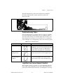
Setting Up Your Imaging System.................................................................................. 3-1
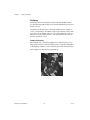
Acquiring Quality Images ............................................................................... 3-3
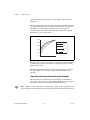
Resolution ......................................................................................... 3-3
Contrast............................................................................................. 3-5
Depth of Field ................................................................................... 3-5
Perspective........................................................................................ 3-5
Distortion .......................................................................................... 3-7
Spatial Calibration ......................................................................................................... 3-7
When to Use.................................................................................................... 3-7
Concepts.......................................................................................................... 3-8
Calibration Process ........................................................................... 3-8
Coordinate System............................................................................ 3-9
Calibration Algorithms ..................................................................... 3-11
Calibration Quality Information ....................................................... 3-12
Image Correction .............................................................................. 3-13
Scaling Mode .................................................................................... 3-14
Correction Region............................................................................. 3-14
Simple Calibration ........................................................................... 3-16
Redefining a Coordinate System ...................................................... 3-17
NI Vision Concepts Manual
vi
ni.com
Contents
PART II
Image Processing and Analysis
Chapter 4
Image Analysis
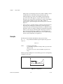
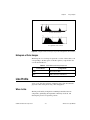
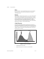
Histogram.......................................................................................................................4-1
When to Use ....................................................................................................4-1
Concepts ..........................................................................................................4-2
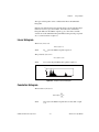
Linear Histogram.............................................................................................4-3
Cumulative Histogram.....................................................................................4-3
Interpretation ...................................................................................................4-4
Histogram Scale...............................................................................................4-4
Histogram of Color Images .............................................................................4-5
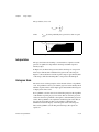
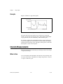
Line Profile ....................................................................................................................4-5
When to Use ....................................................................................................4-5
Concepts ..........................................................................................................4-6
Intensity Measurements .................................................................................................4-6
When to Use ....................................................................................................4-6
Concepts ..........................................................................................................4-7
Chapter 5
Image Processing
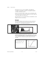
Lookup Tables ...............................................................................................................5-1
When to Use ....................................................................................................5-1
Concepts ..........................................................................................................5-1
Example ............................................................................................5-2
Predefined Lookup Tables ................................................................5-3
Logarithmic and Inverse Gamma Correction....................................5-3
Exponential and Gamma Correction.................................................5-6
Equalize.............................................................................................5-8
Convolution Kernels ......................................................................................................5-10
When to Use ....................................................................................................5-10
Concepts ..........................................................................................................5-10
Spatial Filtering..............................................................................................................5-12
When to Use ....................................................................................................5-13
Concepts ..........................................................................................................5-14
Spatial Filter Types Summary...........................................................5-14
Linear Filters .....................................................................................5-14
Nonlinear Filters ...............................................................................5-27
In-Depth Discussion ........................................................................................5-31
Linear Filters .....................................................................................5-32
© National Instruments Corporation
vii
NI Vision Concepts Manual
Contents
Nonlinear Prewitt Filter .................................................................... 5-33
Nonlinear Sobel Filter ...................................................................... 5-33
Nonlinear Gradient Filter.................................................................. 5-33
Roberts Filter .................................................................................... 5-33
Differentiation Filter......................................................................... 5-34
Sigma Filter ...................................................................................... 5-34
Lowpass Filter .................................................................................. 5-34
Median Filter .................................................................................... 5-34
Nth Order Filter ................................................................................ 5-34
Grayscale Morphology .................................................................................................. 5-35
When to Use.................................................................................................... 5-35
Concepts.......................................................................................................... 5-36
Erosion Function............................................................................... 5-36
Dilation Function .............................................................................. 5-36
Erosion and Dilation Examples ........................................................ 5-36
Opening Function ............................................................................. 5-37
Closing Function............................................................................... 5-38
Opening and Closing Examples ....................................................... 5-38
Proper-Opening Function ................................................................. 5-39
Proper-Closing Function................................................................... 5-39
Auto-Median Function ..................................................................... 5-39
In-Depth Discussion........................................................................................ 5-39
Erosion Concept and Mathematics ................................................... 5-39
Dilation Concept and Mathematics .................................................. 5-40
Proper-Opening Concept and Mathematics...................................... 5-40
Proper-Closing Concept and Mathematics ....................................... 5-41
Auto-Median Concept and Mathematics .......................................... 5-41
Chapter 6
Operators
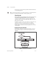
Introduction ................................................................................................................... 6-1
When to Use .................................................................................................................. 6-1
Concepts ........................................................................................................................ 6-1
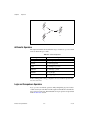
Arithmetic Operators....................................................................................... 6-2
Logic and Comparison Operators ................................................................... 6-2
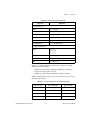
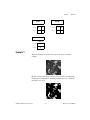
Truth Tables...................................................................................... 6-4
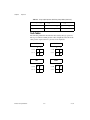
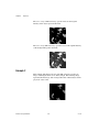
Example 1 ....................................................................................................... 6-5
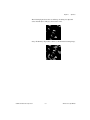
Example 2 ....................................................................................................... 6-6
NI Vision Concepts Manual
viii
ni.com
Contents
Chapter 7
Frequency Domain Analysis
Introduction....................................................................................................................7-1
When to Use...................................................................................................................7-2
Concepts.........................................................................................................................7-3
FFT Representation .........................................................................................7-3
Standard Representation ...................................................................7-3
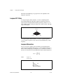
Optical Representation ......................................................................7-4
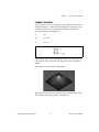
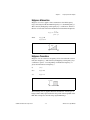
Lowpass FFT Filters........................................................................................7-6
Lowpass Attenuation.........................................................................7-6
Lowpass Truncation ..........................................................................7-7
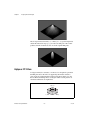
Highpass FFT Filters .......................................................................................7-8
Highpass Attenuation ........................................................................7-9
Highpass Truncation .........................................................................7-9
Mask FFT Filters .............................................................................................7-11
In-Depth Discussion ......................................................................................................7-11
Fourier Transform ...........................................................................................7-11
FFT Display.....................................................................................................7-12
PART III
Particle Analysis
Introduction....................................................................................................................III-1
When to Use...................................................................................................................III-2
Concepts.........................................................................................................................III-2
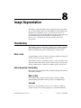
Chapter 8
Image Segmentation
Thresholding ..................................................................................................................8-1
When to Use ....................................................................................................8-1
Global Grayscale Thresholding.......................................................................8-1
When to Use......................................................................................8-1
Concepts............................................................................................8-1
Manual Threshold .............................................................................8-2
Automatic Threshold.........................................................................8-3
Global Color Thresholding..............................................................................8-10
When to Use......................................................................................8-10
Concepts............................................................................................8-10
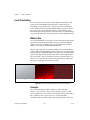
Local Thresholding..........................................................................................8-12
When to Use......................................................................................8-12
Concepts............................................................................................8-12
In-Depth Discussion..........................................................................8-15
© National Instruments Corporation
ix
NI Vision Concepts Manual
Contents
Thresholding Considerations .......................................................................... 8-15
Morphological Segmentation ........................................................................................ 8-16
When to Use.................................................................................................... 8-16
Concepts.......................................................................................................... 8-16
Watershed Transform...................................................................................... 8-19
In-Depth Discussion ......................................................................... 8-20
Chapter 9
Binary Morphology
Introduction ................................................................................................................... 9-1
Structuring Elements ..................................................................................................... 9-1
When to Use.................................................................................................... 9-1
Concepts.......................................................................................................... 9-2
Structuring Element Size .................................................................. 9-2
Structuring Element Values.............................................................. 9-3
Pixel Frame Shape ............................................................................ 9-4
Connectivity .................................................................................................................. 9-7
When to Use.................................................................................................... 9-7
Concepts.......................................................................................................... 9-7
In-Depth Discussion........................................................................................ 9-8
Connectivity-4 .................................................................................. 9-9
Connectivity-8 .................................................................................. 9-9
Primary Morphology Operations................................................................................... 9-9
When to Use.................................................................................................... 9-10
Concepts.......................................................................................................... 9-10
Erosion and Dilation Functions ........................................................ 9-10
Opening and Closing Functions ....................................................... 9-13
Inner Gradient Function.................................................................... 9-14
Outer Gradient Function ................................................................... 9-14
Hit-Miss Function............................................................................. 9-14
Thinning Function ............................................................................ 9-16
Thickening Function......................................................................... 9-18
Proper-Opening Function ................................................................. 9-19
Proper-Closing Function................................................................... 9-20
Auto-Median Function ..................................................................... 9-21
Advanced Morphology Operations ............................................................................... 9-21
When to Use.................................................................................................... 9-21
Concepts.......................................................................................................... 9-22
Border Function ................................................................................ 9-22
Hole Filling Function........................................................................ 9-22
Labeling Function............................................................................. 9-22
Lowpass and Highpass Filters .......................................................... 9-23
Separation Function .......................................................................... 9-24
NI Vision Concepts Manual
x
ni.com
Contents
Skeleton Functions ............................................................................9-25
Segmentation Function .....................................................................9-27
Distance Function .............................................................................9-28
Danielsson Function..........................................................................9-28
Circle Function..................................................................................9-30
Convex Hull Function .......................................................................9-31
Chapter 10
Particle Measurements
Introduction....................................................................................................................10-1
When to Use ....................................................................................................10-1
Pixel Measurements versus Real-World Measurements .................................10-1
Particle Measurements ...................................................................................................10-2
Particle Concepts .............................................................................................10-3
Particle Holes ....................................................................................10-5
Coordinates......................................................................................................10-7
Lengths ............................................................................................................10-9
Areas................................................................................................................10-13
Quantities.........................................................................................................10-14
Angles..............................................................................................................10-14
Ratios...............................................................................................................10-16
Factors .............................................................................................................10-16
Sums ................................................................................................................10-17
Moments ..........................................................................................................10-18
PART IV
Machine Vision
Chapter 11
Edge Detection
Introduction....................................................................................................................11-1
When to Use...................................................................................................................11-1
Gauging ...........................................................................................................11-2
Detection .........................................................................................................11-2
Alignment .......................................................................................................11-3
Concepts.........................................................................................................................11-4
Definition of an Edge ......................................................................................11-4
Characteristics of an Edge ...............................................................................11-5
Edge Detection Methods .................................................................................11-6
Simple Edge Detection......................................................................11-7
Advanced Edge Detection.................................................................11-7
© National Instruments Corporation
xi
NI Vision Concepts Manual
Contents
Subpixel Accuracy............................................................................ 11-9
Extending Edge Detection to 2D Search Regions .......................................... 11-10
Rake .................................................................................................. 11-10
Spoke ................................................................................................ 11-11
Concentric Rake ............................................................................... 11-12
Chapter 12
Pattern Matching
Introduction ................................................................................................................... 12-1
When to Use .................................................................................................................. 12-1
What to Expect from a Pattern Matching Tool ............................................................. 12-2
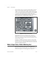
Pattern Orientation and Multiple Instances..................................................... 12-3
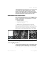
Ambient Lighting Conditions ......................................................................... 12-3
Blur and Noise Conditions .............................................................................. 12-4
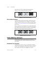
Pattern Matching Techniques ........................................................................................ 12-4
Normalized Cross-Correlation ........................................................................ 12-4
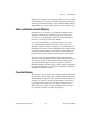
Scale- and Rotation-Invariant Matching ......................................................... 12-5
Pyramidal Matching ........................................................................................ 12-5
Image Understanding ...................................................................................... 12-6
In-Depth Discussion ...................................................................................................... 12-7
Normalized Cross-Correlation ........................................................................ 12-7
Chapter 13
Geometric Matching
Introduction ................................................................................................................... 13-1
When to Use .................................................................................................................. 13-1
When Not to Use Geometric Matching........................................................... 13-4
What to Expect from a Geometric Matching Tool........................................................ 13-5
Part Quantity, Orientation, and Size ............................................................... 13-5
Non-Linear or Non-Uniform Lighting Conditions ......................................... 13-6
Contrast Reversal ............................................................................................ 13-6
Partial Occlusion ............................................................................................. 13-7
Different Image Backgrounds ......................................................................... 13-8
Geometric Matching Technique .................................................................................... 13-8
Learning .......................................................................................................... 13-9
Curve Extraction............................................................................... 13-9
Feature Extraction............................................................................. 13-12
Representation of Spatial Relationships ........................................... 13-13
Matching ......................................................................................................... 13-13
Feature Correspondence Matching ................................................... 13-13
Template Model Matching ............................................................... 13-13
Match Refinement ............................................................................ 13-14
NI Vision Concepts Manual
xii
ni.com
Contents
Geometric Matching Using Calibrated Images .............................................................13-14
Simple Calibration or Previously Corrected Images .......................................13-14
Perspective or Nonlinear Distortion Calibration .............................................13-14
In-Depth Discussion ......................................................................................................13-15
Geometric Matching Report ............................................................................13-15
Score..................................................................................................13-15
Template Target Curve Score ...........................................................13-16
Target Template Curve Score ...........................................................13-17
Correlation Score ..............................................................................13-18
Chapter 14
Dimensional Measurements
Introduction....................................................................................................................14-1
When to Use...................................................................................................................14-1
Concepts.........................................................................................................................14-2
Locating the Part in the Image.........................................................................14-2
Locating Features ...........................................................................................14-2
Making Measurements ....................................................................................14-2
Qualifying Measurements ...............................................................................14-3
Coordinate System .........................................................................................................14-3
When to Use ....................................................................................................14-4
Concepts ..........................................................................................................14-4
In-Depth Discussion ........................................................................................14-5
Edge-Based Coordinate System Functions .......................................14-5
Pattern Matching-Based Coordinate System Functions....................14-8
Finding Features or Measurement Points ......................................................................14-10
Edge-Based Features .......................................................................................14-10
Line and Circular Features ..............................................................................14-11
Shape-Based Features......................................................................................14-12
Making Measurements on the Image.............................................................................14-13
Distance Measurements...................................................................................14-13
Analytic Geometry ..........................................................................................14-14
Line Fitting........................................................................................14-15
Chapter 15
Color Inspection
Color Spaces ..................................................................................................................15-1
When to Use ....................................................................................................15-1
Concepts ..........................................................................................................15-2
RGB Color Space..............................................................................15-3
HSL Color Space ..............................................................................15-5
CIE XYZ Color Space ......................................................................15-5
© National Instruments Corporation
xiii
NI Vision Concepts Manual
Contents
CIE L*a*b* Color Space .................................................................. 15-7
CMY Color Space ............................................................................ 15-8
YIQ Color Space .............................................................................. 15-8
Color Spectrum.............................................................................................................. 15-8
Color Space Used to Generate the Spectrum .................................................. 15-8
Generating the Color Spectrum....................................................................... 15-10
Color Matching.............................................................................................................. 15-12
When to Use.................................................................................................... 15-13
Color Identification........................................................................... 15-13
Color Inspection ............................................................................... 15-14
Concepts.......................................................................................................... 15-15
Learning Color Distribution ............................................................. 15-16
Comparing Color Distributions ........................................................ 15-16
Color Location............................................................................................................... 15-17
When to Use.................................................................................................... 15-17
Inspection.......................................................................................... 15-17
Identification..................................................................................... 15-18
What to Expect from a Color Location Tool .................................................. 15-19
Pattern Orientation and Multiple Instances ...................................... 15-20
Ambient Lighting Conditions ........................................................... 15-20
Blur and Noise Conditions ............................................................... 15-21
Concepts.......................................................................................................... 15-21
Color Pattern Matching ................................................................................................. 15-23
When to Use.................................................................................................... 15-23
What to Expect from a Color Pattern Matching Tool ..................................... 15-26
Pattern Orientation and Multiple Instances ...................................... 15-26
Ambient Lighting Conditions ........................................................... 15-27
Blur and Noise Conditions ............................................................... 15-28
Concepts.......................................................................................................... 15-28
Color Matching and Color Location................................................. 15-28
Grayscale Pattern Matching.............................................................. 15-29
Combining Color Location and Grayscale Pattern Matching .......... 15-29
In-Depth Discussion........................................................................................ 15-30
RGB to Grayscale ............................................................................. 15-31
RGB and HSL................................................................................... 15-31
RGB and CIE XYZ........................................................................... 15-32
RGB and CIE L*a*b*....................................................................... 15-34
RGB and CMY ................................................................................. 15-35
RGB and YIQ ................................................................................... 15-35
NI Vision Concepts Manual
xiv
ni.com
Contents
Chapter 16
Binary Particle Classification
Introduction....................................................................................................................16-1
When to Use ....................................................................................................16-1
Ideal Images for Classification........................................................................16-2
General Classification Procedure ....................................................................16-3
Training the Particle Classifier ......................................................................................16-6
Classifying Samples.......................................................................................................16-7
Preprocessing...................................................................................................16-8
Feature Extraction ...........................................................................................16-8
Invariant Features..............................................................................16-9
Classification ...................................................................................................16-9
Classification Methods ..................................................................................................16-9
Instance-Based Learning .................................................................................16-9
Nearest Neighbor Classifier ..............................................................16-10
K-Nearest Neighbor Classifier..........................................................16-11
Minimum Mean Distance Classifier .................................................16-12
Multiple Classifier System ..............................................................................16-13
Cascaded Classification System........................................................16-13
Parallel Classification Systems .........................................................16-13
Custom Classification ....................................................................................................16-14
When to Use ....................................................................................................16-14
Concepts ..........................................................................................................16-14
In-Depth Discussion ......................................................................................................16-14
Training Feature Data Evaluation ...................................................................16-14
Intraclass Deviation Array ................................................................16-15
Class Distance Table.........................................................................16-16
Determining the Quality of a Trained Classifier .............................................16-16
Classifier Predictability.....................................................................16-16
Classifier Accuracy ...........................................................................16-17
Identification and Classification Score............................................................16-18
Classification Confidence .................................................................16-18
Identification Confidence..................................................................16-18
Calculating Example Classification and Identification
Confidences....................................................................................16-19
Evaluating Classifier Performance....................................................16-20
© National Instruments Corporation
xv
NI Vision Concepts Manual
Contents
Chapter 17
Golden Template Comparison
Introduction ................................................................................................................... 17-1
When to Use .................................................................................................................. 17-1
Concepts ........................................................................................................................ 17-1
Alignment........................................................................................................ 17-2
Perspective Correction .................................................................................... 17-3
Histogram Matching ....................................................................................... 17-4
Ignoring Edges ................................................................................................ 17-5
Using Defect Information for Inspection ........................................................ 17-6
Chapter 18
Optical Character Recognition
Introduction ................................................................................................................... 18-1
When to Use .................................................................................................................. 18-2
Training Characters ....................................................................................................... 18-2
Reading Characters........................................................................................................ 18-4
OCR Session.................................................................................................................. 18-6
Concepts and Terminology............................................................................................ 18-6
Region of Interest (ROI) ................................................................................. 18-6
Particles, Elements, Objects, and Characters .................................................. 18-6
Patterns............................................................................................................ 18-7
Character Segmentation .................................................................................. 18-7
Thresholding ..................................................................................... 18-7
Threshold Limits............................................................................... 18-9
Character Spacing............................................................................. 18-9
Element Spacing ............................................................................... 18-9
Character Bounding Rectangle ......................................................... 18-11
AutoSplit........................................................................................... 18-11
Character Size................................................................................... 18-11
Substitution Character..................................................................................... 18-11
Acceptance Level............................................................................................ 18-11
Read Strategy .................................................................................................. 18-12
Read Resolution .............................................................................................. 18-12
Valid Characters.............................................................................................. 18-12
Aspect Ratio Independence............................................................................. 18-13
OCR Scores..................................................................................................... 18-13
Classification Score .......................................................................... 18-13
Verification Score............................................................................. 18-13
Removing Small Particles ............................................................................... 18-14
Removing Particles That Touch the ROI ........................................................ 18-14
NI Vision Concepts Manual
xvi
ni.com
Contents
Chapter 19
Instrument Readers
Introduction....................................................................................................................19-1
When to Use ....................................................................................................19-1
Meter Functions .............................................................................................................19-1
Meter Algorithm Limits ..................................................................................19-2
LCD Functions...............................................................................................................19-2
LCD Algorithm Limits ....................................................................................19-2
Barcode Functions .........................................................................................................19-3
Barcode Algorithm Limits...............................................................................19-3
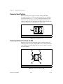
2D Barcode Functions ...................................................................................................19-4
Data Matrix......................................................................................................19-5
Quality Grading.................................................................................19-5
PDF417............................................................................................................19-10
2D Barcode Algorithm Limits.........................................................................19-10
Appendix A
Kernels
Appendix B
Technical Support and Professional Services
Glossary
Index
© National Instruments Corporation
xvii
NI Vision Concepts Manual
About This Manual
The NI Vision Concepts Manual helps people with little or no imaging
experience learn the basic concepts of machine vision and image
processing. This manual also contains in-depth discussions on machine
vision and image processing functions for advanced users.
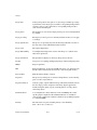
Conventions
The following conventions appear in this manual:
»
The » symbol leads you through nested menu items and dialog box options
to a final action. The sequence File»Page Setup»Options directs you to
pull down the File menu, select the Page Setup item, and select Options
from the last dialog box.
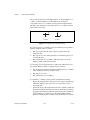
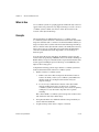
This icon denotes a tip, which alerts you to advisory information.
This icon denotes a note, which alerts you to important information.
bold
Bold text denotes items that you must select or click in the software, such
as menu items and dialog box options. Bold text also denotes parameter
names.
italic
Italic text denotes variables, emphasis, a cross reference, or an introduction
to a key concept. Italic text also denotes text that is a placeholder for a word
or value that you must supply.
monospace
Text in this font denotes text or characters that you should enter from the
keyboard, sections of code, programming examples, and syntax examples.
This font is also used for the proper names of disk drives, paths, directories,
programs, subprograms, subroutines, device names, functions, operations,
variables, filenames, and extensions.
Related Documentation
The following documents contain information that you might find helpful
as you read this manual:
•
© National Instruments Corporation
NI Vision for LabVIEW User Manual—Contains information about
how to build a vision application using NI Vision for LabVIEW.
xix
NI Vision Concepts Manual
About This Manual
NI Vision Concepts Manual
•
NI Vision for LabWindows™/CVI™ User Manual—Contains
information about how to build a vision application using NI Vision
for LabWindows/CVI.
•
NI Vision for Visual Basic User Manual—Contains information about
how to build a vision application using NI Vision for Visual Basic.
•
NI Vision for LabVIEW VI Reference Help—Contains reference
information about NI Vision for LabVIEW palettes and VIs.
•
NI Vision for LabWindows/CVI Function Reference Help—Contains
reference information about NI Vision functions for
LabWindows/CVI.
•
NI Vision for Visual Basic Reference Help—Contains reference
information about NI Vision for Visual Basic.
•
NI Vision Assistant Tutorial—Describes the NI Vision Assistant
software interface and guides you through creating example image
processing and machine vision applications.
•
NI Vision Assistant Help—Contains descriptions of the NI Vision
Assistant features and functions and provides instructions for using
them.
•
NI Vision Builder for Automated Inspection Tutorial—Describes
Vision Builder for Automated Inspection and provides step-by-step
instructions for solving common visual inspection tasks, such as
inspection, gauging, part presence, guidance, and counting.
•
NI Vision Builder for Automated Inspection: Configuration
Help—Contains information about using the Vision Builder for
Automated Inspection Configuration Interface to create a machine
vision application.
xx
ni.com
Part I
Vision Basics
This section describes conceptual information about digital images, image
display, and system calibration.
Part I, Vision Basics, contains the following chapters:
Chapter 1, Digital Images, contains information about the properties of
digital images, image types, file formats, the internal representation of
images in NI Vision, image borders, and image masks.
Chapter 2, Display, contains information about image display, palettes,
regions of interest, and nondestructive overlays.
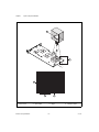
Chapter 3, System Setup and Calibration, describes how to set up an
imaging system and calibrate the imaging setup so that you can convert
pixel coordinates to real-world coordinates.
© National Instruments Corporation
I-1
NI Vision Concepts Manual
1
Digital Images
This chapter contains information about the properties of digital images,
image types, file formats, the internal representation of images in
NI Vision, image borders, and image masks.
Definition of a Digital Image
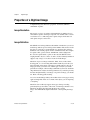
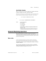
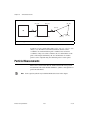
An image is a 2D array of values representing light intensity. For the
purposes of image processing, the term image refers to a digital image.
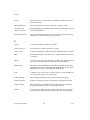
An image is a function of the light intensity
f(x, y)
where f is the brightness of the point (x, y), and x and y represent the spatial
coordinates of a picture element, or pixel.
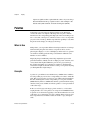
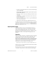
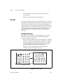
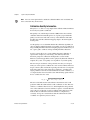
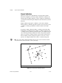
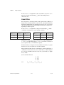
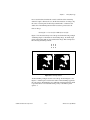
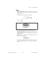
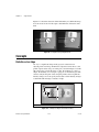
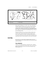
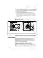
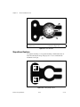
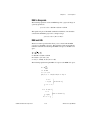
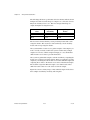
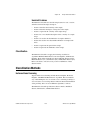
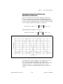
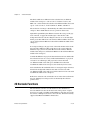
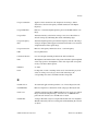
By convention, the spatial reference of the pixel with the coordinates (0, 0)
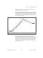
is located at the top, left corner of the image. Notice in Figure 1-1 that the
value of x increases moving from left to right, and the value of y increases
from top to bottom.
(0,0)
X
f ( x, y )
Y
Figure 1-1. Spatial Reference of the (0, 0) Pixel
In digital image processing, an imaging sensor converts an image into a
discrete number of pixels. The imaging sensor assigns to each pixel a
numeric location and a gray level or color value that specifies the brightness
or color of the pixel.
© National Instruments Corporation
1-1
NI Vision Concepts Manual
Chapter 1
Digital Images
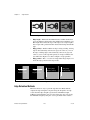
Properties of a Digitized Image
A digitized image has three basic properties: resolution, definition,
and number of planes.
Image Resolution
The spatial resolution of an image is determined by its number of rows
and columns of pixels. An image composed of m columns and n rows has
a resolution of m × n. This image has m pixels along its horizontal axis
and n pixels along its vertical axis.
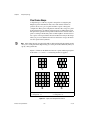
Image Definition
The definition of an image indicates the number of shades that you can see
in the image. The bit depth of an image is the number of bits used to encode
the value of a pixel. For a given bit depth of n, the image has an image
definition of 2n, meaning a pixel can have 2n different values. For example,
if n equals 8 bits, a pixel can have 256 different values ranging from
0 to 255. If n equals 16 bits, a pixel can have 65,536 different values
ranging from 0 to 65,535 or from –32,768 to 32,767. Currently, NI Vision
supports only a range of –32,768 to 32,767 for 16-bit images.
NI Vision can process images with 8-bit, 10-bit, 12-bit, 14-bit, 16-bit,
floating point, or color encoding. The manner in which you encode your
image depends on the nature of the image acquisition device, the type of
image processing you need to use, and the type of analysis you need to
perform. For example, 8-bit encoding is sufficient if you need to obtain the
shape information of objects in an image. However, if you need to precisely
measure the light intensity of an image or region in an image, you should
use 16-bit or floating-point encoding.
Use color encoded images when your machine vision or image processing
application depends on the color content of the objects you are inspecting
or analyzing.
NI Vision does not directly support other types of image encoding,
particularly images encoded as 1-bit, 2-bit, or 4-bit images. In these cases,
NI Vision automatically transforms the image into an 8-bit
image—the minimum bit depth for NI Vision—when opening the image
file.
NI Vision Concepts Manual
1-2
ni.com
Chapter 1
Digital Images
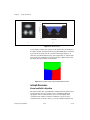
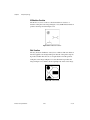
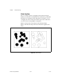
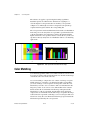
Number of Planes
The number of planes in an image corresponds to the number of arrays
of pixels that compose the image. A grayscale or pseudo-color image
is composed of one plane. A true-color image is composed of
three planes—one each for the red component, blue component, and
green component.
In true-color images, the color component intensities of a pixel are coded
into three different values. A color image is the combination of three arrays
of pixels corresponding to the red, green, and blue components in an RGB
image. HSL images are defined by their hue, saturation, and luminance
values.
Image Types
The NI Vision libraries can manipulate three types of images: grayscale,
color, and complex images. Although NI Vision supports all three image
types, certain operations on specific image types are not possible. For
example, you cannot apply the logic operator AND to a complex image.
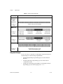
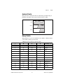
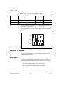
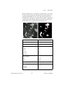
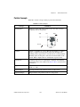
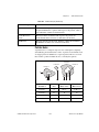
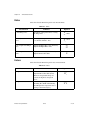
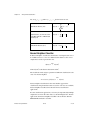
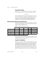
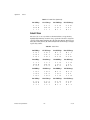
Table 1-1 shows how many bytes per pixel grayscale, color, and complex
images use. For an identical spatial resolution, a color image occupies
four times the memory space of an 8-bit grayscale image, and a complex
image occupies eight times the memory of an 8-bit grayscale image.
Table 1-1. Bytes per Pixel
Image Type
Number of Bytes per Pixel Data
8-bit
(Unsigned)
Integer
Grayscale
(1 byte or
8-bit)
8-bit for the grayscale intensity
16-bit
(Signed)
Integer
Grayscale
(2 bytes or
16-bit)
© National Instruments Corporation
16-bit for the grayscale intensity
1-3
NI Vision Concepts Manual
Chapter 1
Digital Images
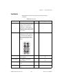
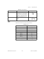
Table 1-1. Bytes per Pixel (Continued)
Image Type
Number of Bytes per Pixel Data
32-bit
FloatingPoint
Grayscale
(4 bytes or
32-bit)
32-bit for the grayscale intensity
RGB Color
(4 bytes or
32-bit)
8-bit for the
alpha value
(not used)
8-bit for the
red intensity
8-bit for the
green intensity
8-bit for the
blue intensity
8-bit not used
8-bit for the hue
8-bit for the
saturation
8-bit for the
luminance
HSL Color
(4 bytes or
32-bit)
Complex
(8 bytes or
64-bit)
32-bit floating for the real part
32-bit for the imaginary part
Grayscale Images
A grayscale image is composed of a single plane of pixels. Each pixel is
encoded using one of the following single numbers:
NI Vision Concepts Manual
•
An 8-bit unsigned integer representing grayscale values between
0 and 255
•
A 16-bit signed integer representing grayscale values between
–32,768 and +32,767
•
A single-precision floating point number, encoded using four bytes,
representing grayscale values ranging from –∞ to ∞
1-4
ni.com
Chapter 1
Digital Images
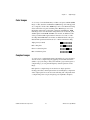
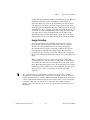
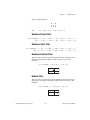
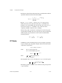
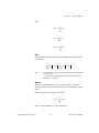
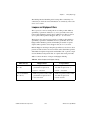
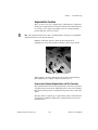
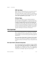
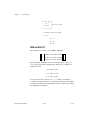
Color Images
A color image is encoded in memory as either a red, green, and blue (RGB)
image or a hue, saturation, and luminance (HSL) image. Color image pixels
are a composite of four values. RGB images store color information using
8 bits each for the red, green, and blue planes. HSL images store color
information using 8 bits each for hue, saturation, and luminance. RGB
U64 images store color information using 16 bits each for the red, green,
and blue planes. In the RGB and HSL color models, an additional 8-bit
value goes unused. This representation is known as 4 × 8-bit or 32-bit
encoding. In the RGB U64 color model, an additional 16-bit value goes
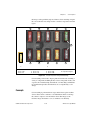
unused. This representation is known as 4 × 16-bit or 64-bit encoding.
Alpha plane (not used)
Red or hue plane
Green or saturation plane
Blue or luminance plane
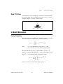
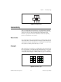
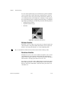
Complex Images
A complex image contains the frequency information of a grayscale image.
You can create a complex image by applying a Fast Fourier transform
(FFT) to a grayscale image. After you transform a grayscale image into a
complex image, you can perform frequency domain operations on the
image.
Each pixel in a complex image is encoded as two single-precision
floating-point values, which represent the real and imaginary components
of the complex pixel. You can extract the following four components from
a complex image: the real part, imaginary part, magnitude, and phase.
© National Instruments Corporation
1-5
NI Vision Concepts Manual
Chapter 1
Digital Images
Image Files
An image file is composed of a header followed by pixel values. Depending
on the file format, the header contains image information about the
horizontal and vertical resolution, pixel definition, and the original palette.
Image files may also store information about calibration, pattern matching
templates, and overlays. The following are common image file formats:
•
Bitmap (BMP)
•
Tagged image file format (TIFF)
•
Portable network graphics (PNG)—Offers the capability of storing
image information about spatial calibration, pattern matching
templates, and overlays
•
Joint Photographic Experts Group format (JPEG)
•
National Instruments internal image file format (AIPD)—Used for
saving floating-point, complex, and HSL images
Standard formats for 8-bit grayscale and RGB color images are BMP,
TIFF, PNG, JPEG, and AIPD. Standard formats for 16-bit grayscale, 64-bit
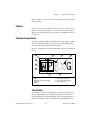
RGB, and complex images are PNG and AIPD.
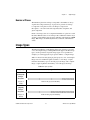
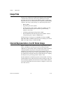
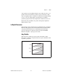
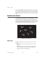
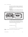
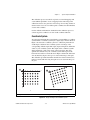
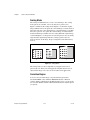
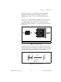
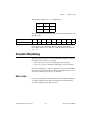
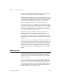
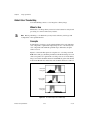
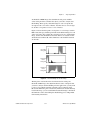
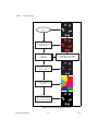
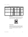
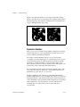
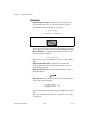
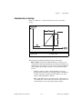
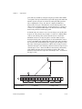
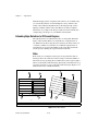
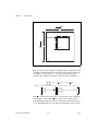
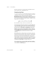
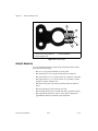
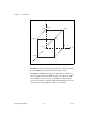
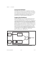
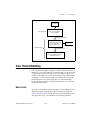
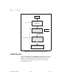
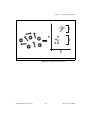
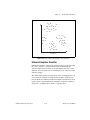
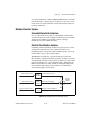
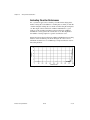
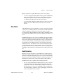
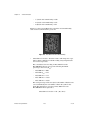
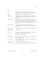
Internal Representation of an NI Vision Image
Figure 1-2 illustrates how an NI Vision image is represented in system
memory. In addition to the image pixels, the stored image includes
additional rows and columns of pixels called the image border and the left
and right alignments. Specific processing functions involving pixel
neighborhood operations use image borders. The alignment regions ensure
that the first pixel of the image is 32-byte aligned in memory. The size of
the alignment blocks depend on the image width and border size. Aligning
the image increases processing speed by as much as 30%.
The line width is the total number of pixels in a horizontal line of an image,
which includes the sum of the horizontal resolution, the image borders, and
the left and right alignments. The horizontal resolution and line width may
be the same length if the horizontal resolution is a multiple of 32 bytes and
the border size is 0.
NI Vision Concepts Manual
1-6
ni.com
Chapter 1
Digital Images
7
4
2
5
2
6
2
1
3
2
1
2
Image
Image Border
3
4
Vertical Resolution
Left Alignment
5
6
Horizontal Resolution
Right Alignment
7
Line Width
Figure 1-2. Internal Image Representation
© National Instruments Corporation
1-7
NI Vision Concepts Manual
Chapter 1
Digital Images
Image Borders
Many image processing functions process a pixel by using the values of its
neighbors. A neighbor is a pixel whose value affects the value of a nearby
pixel when an image is processed. Pixels along the edge of an image do not
have neighbors on all four sides. If you need to use a function that processes
pixels based on the value of their neighboring pixels, specify an image
border that surrounds the image to account for these outlying pixels.
You define the image border by specifying a border size and the values of
the border pixels.
The size of the border should accommodate the largest pixel neighborhood
required by the function you are using. The size of the neighborhood is
specified by the size of a 2D array. For example, if a function uses the
eight adjoining neighbors of a pixel for processing, the size of the
neighborhood is 3 × 3, indicating an array with three columns and
three rows. Set the border size to be greater than or equal to half the number
of rows or columns of the 2D array rounded down to the nearest integer
value. For example, if a function uses a 3 × 3 neighborhood, the image
should have a border size of at least 1; if a function uses a 5 × 5
neighborhood, the image should have a border size of at least 2. In NI
Vision, an image is created with a default border size of 3, which can
support any function using up to a 7 × 7 neighborhood without any
modification.
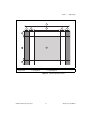
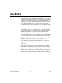
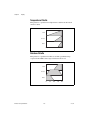
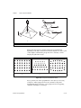
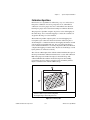
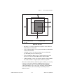
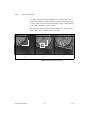
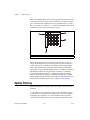
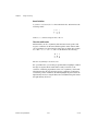
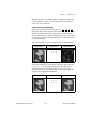
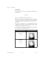
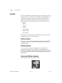
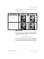
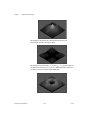
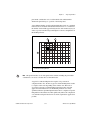
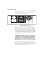
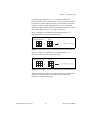
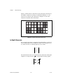
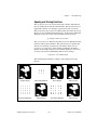
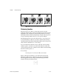
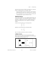
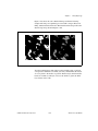
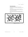
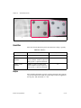
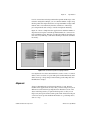
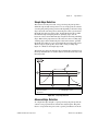
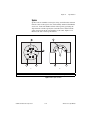
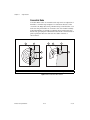
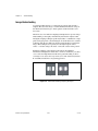
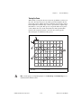
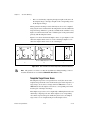
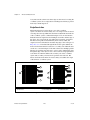
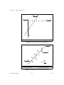
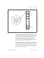
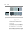
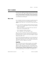
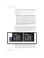
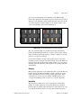
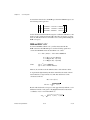
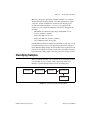
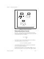
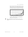
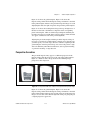
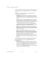
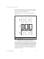
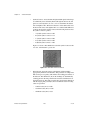
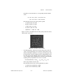
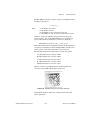
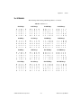
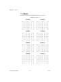
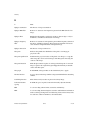
NI Vision provides three ways to specify the pixel values of the image
border. Figure 1-3 illustrates these options. Figure 1-3a shows the pixel
values of an image. By default, all image border pixels have a value of 0, as
shown in Figure 1-3b. You can copy the values of the pixels along the edge
of the image into the border pixels, as shown in Figure 1-3c, or you can
mirror the pixel values along the edge of the image into the border pixels,
as shown in Figure 1-3d.
NI Vision Concepts Manual
1-8
ni.com
Chapter 1
Digital Images
20 20 20 20 20 20 20 20 20 20 20 20 20 20
0
0 20
0 20
0 20
0 20
0 20
0 20
0 20
0 20
0 20
0 20
0 0
0
20 20 20 20 20 20 20 20 20 20 20 20 20 20
0
0 20
0 20
0 20
0 20
0 20
0 20
0 20
0 20
0 20
0 20
0 0
0
20 20 10 9 15 11 12 20 16 12 11 8 20 20
0
0 10 9 15 11 12 20 16 12 11 8
0
0
20 20 11 13 11 12 9 16 17 11 13 14 20 20
0
0 11 13 11 12 9 16 17 11 13 14 0
0
20 20 12 8 12 14 12 13 12 14 11 13 20 20
0
0 12 8 12 14 12 13 12 14 11 13 0
0
20 20 10 9 13 31 30 32 33 12 13 11 20 20
0
0 10 9 13 31 30 32 33 12 13 11 0
0
20 20 15 11 10 30 42 45 31 15 12 10 20 20
0
0 15 11 10 30 42 45 31 15 12 10 0
0
20 20 13 12 14 29 40 41 33 13 12 13 20 20
0
0 13 12 14 29 40 41 33 13 12 13 0
0
20 20 14 15 12 33 34 36 32 12 14 11 20 20
0
0 14 15 12 33 34 36 32 12 14 11 0
0
20 20 10 12 13 14 12 16 12 15 10 9 20 20
0
0 10 12 13 14 12 16 12 15 10 9
0
0
20 20 10 8 11 13 15 17 13 14 12 10 20 20
0
0 10 8 11 13 15 17 13 14 12 10 0
0
20 20 9 10 12 11 8 15 14 12 11 7 20 20
0
0
0
9 10 12 11 8 15 14 12 11 7
0
20 20 20 20 20 20 20 20 20 20 20 20 20 20
0
0
0
0
0
0
0
0
0
0
0
0
0
0
20 20 20 20 20 20 20 20 20 20 20 20 20 20
0
0
0
0
0
0
0
0
0
0
0
0
0
0
b.
a.
10 10 10 9 15 11 12 20 16 22 11 8
8
8
13 11 11 13 11 12 9 16 17 11 13 14 14 13
10 10 10 9 15 11 12 20 16 22 11 8
8
8
9 10 10 9 15 11 12 20 16 12 11 8
8 11
10 10 10 9 15 11 12 20 16 12 11 8
8
8
9 10 10 9 15 11 12 20 16 12 11 8
8 11
13 11 11 13 11 12 9 16 17 11 13 14 14 13
11 11 11 13 11 12 9 16 17 11 13 14 14 14
12 12 12 8 12 14 12 13 12 14 11 13 13 13
8 12 12 8 12 14 12 13 12 14 11 13 13 11
10 10 10 9 13 31 30 32 33 12 13 11 11 11
9 10 10 9 13 31 30 32 33 12 13 11 11 13
15 15 15 11 10 30 42 45 31 15 12 10 10 10
11 15 15 11 10 30 42 45 31 15 12 10 10 12
13 13 13 12 14 29 40 41 33 13 12 13 13 13
12 13 13 12 14 29 40 41 33 13 12 13 13 12
14 14 14 15 12 33 34 36 32 12 14 11 11 11
15 14 14 15 12 33 34 36 32 12 14 11 11 14
10 10 10 12 13 14 12 16 12 15 10 9
12 10 10 12 13 14 12 16 12 15 10 9
9
9
9 10
10 10 10 8 11 13 15 17 13 14 12 10 10 10
8 10 10 8 11 13 15 17 13 14 12 10 10 12
9
9
9 10 12 11 8 15 14 12 11 7
7
7
10 9
9 10 12 11 8 15 14 12 11 7
7 11
9
9
9 10 12 11 8 15 14 12 11 7
7
7
10 9
9 10 12 11 8 15 14 12 11 7
7 11
9
9
9 10 12 11 8 15 14 12 11 7
7
7
8 10 10 8 11 13 15 17 13 14 12 10 10 12
d.
c.
Figure 1-3. Setting the Pixel Values of an Image Border
The method you use to fill the border pixels depends on the processing
function you require for your application. Review how the function works
before choosing a border-filling method because your choice can
drastically affect the processing results. For example, if you are using a
function that detects edges in an image based on the difference between a
pixel and its neighbors, do not set the border pixel values to zero. As shown
in Figure 1-3b, an image border containing zero values introduces
significant differences between the pixel values in the border and the image
pixels along the border, which causes the function to detect erroneous edges
along the border of the image. If you are using an edge detection function,
copy or mirror the pixel values along the border into the border region to
obtain more accurate results.
© National Instruments Corporation
1-9
NI Vision Concepts Manual
Chapter 1
Digital Images
In NI Vision, most image processing functions that use neighbors
automatically set pixel values in the image border using neighborhoods.
The grayscale filtering operations low pass, Nth order, and edge detection
use the mirroring method to set pixels in the image border. The binary
morphology, grayscale morphology, and segmentation functions copy the
pixel values along the border into the border region. The correlate, circles,
reject border, remove particles, skeleton, and label functions set the pixel
values in the border to zero.
Note The border of an image is taken into account only for processing. The border is never
displayed or stored in a file.
Image Masks
An image mask isolates parts of an image for processing. If a function has
an image mask parameter, the function process or analysis depends on both
the source image and the image mask.
An image mask is an 8-bit binary image that is the same size as or smaller
than the inspection image. Pixels in the image mask determine whether
corresponding pixels in the inspection image are processed. If a pixel in the
image mask has a nonzero value, the corresponding pixel in the inspection
image is processed. If a pixel in the image mask has a value of 0, the
corresponding pixel in the inspection image is not processed.
When to Use
Use image masks when you want to focus your processing or inspection on
particular regions in the image.
Concepts
Pixels in the source image are processed if corresponding pixels in the
image mask have values other than zero. Figure 1-4 shows how a mask
affects the output of the function that inverts the pixel values in an image.
Figure 1-4a shows the inspection image. Figure 1-4b shows the image
mask. Pixels in the mask with zero values are represented in black, and
pixels with nonzero values are represented in white. Figure 1-4c shows the
inverse of the inspection image using the image mask. Figure 1-4d shows
the inverse of the inspection image without the image mask.
NI Vision Concepts Manual
1-10
ni.com
Chapter 1
a.
b.
c.
Digital Images
d.
Figure 1-4. The Effect of an Image Mask
You can limit the area in which your function applies an image mask to
the bounding rectangle of the region you want to process. This technique
saves memory by limiting the image mask to only the part of the image
containing significant information. To keep track of the location of this
region of interest (ROI) in regard to the original image, NI Vision sets an
offset. An offset defines the coordinate position in the original image where
you want to place the origin of the image mask.
Figure 1-5 illustrates the different methods of applying image masks.
Figure 1-5a shows the ROI in which you want to apply an image mask.
Figure 1-5b shows an image mask with the same size as the inspection
image. In this case, the offset is set to [0, 0]. A mask image also can be the
size of the bounding rectangle of the ROI, as shown in Figure 1-5c, where
the offset specifies the location of the mask image in the reference image.
You can define this offset to apply the mask image to different regions in
the inspection image.
1
a.
1
1
1
2
2
b.
Region of Interest
2
c.
Image Mask
Figure 1-5. Using an Offset to Limit an Image Mask
Figure 1-6 illustrates the use of a mask with two different offsets.
Figure 1-6a shows the inspection image, and Figure 1-6b shows the image
mask. Figure 1-6c and Figure 1-6d show the results of a function using the
image mask given the offsets of [0, 0] and [3, 1], respectively.
© National Instruments Corporation
1-11
NI Vision Concepts Manual
Chapter 1
Digital Images
a.
b.
c.
d.
Border pixels
Pixels not affected by the mask
Pixels affected by the mask
Figure 1-6. Effect of Applying a Mask with Different Offsets
For more information about ROIs, refer to the Regions of Interest section
of Chapter 2, Display.
NI Vision Concepts Manual
1-12
ni.com
2
Display
This chapter contains information about image display, palettes, regions of
interest, and nondestructive overlays.
Image Display
Displaying images is an important component of a vision application
because it gives you the ability to visualize your data. Image processing
and image visualization are distinct and separate elements. Image
processing refers to the creation, acquisition, and analysis of images.
Image visualization refers to how image data is presented and how you
can interact with the visualized images. A typical imaging application
uses many images in memory that the application never displays.
When to Use
Use display functions to visualize your image data, retrieve generated
events and the associated data from an image display environment, select
ROIs from an image interactively, and annotate the image with additional
information.
Concepts
Depending on your application development environment, you can display
images in the following image display environments: an external window
(LabVIEW and LabWindows/CVI), the LabVIEW Image Display control
(LabVIEW 7.0 or later), and the CWIMAQViewer ActiveX control
(Visual Basic). Display functions display images, set attributes of the
image display environment, assign color palettes to image display
environments, close image display environments, and set up and use an
image browser in image display environments. Some ROI functions—a
subset of the display functions—interactively define ROIs in image display
environments. These ROI functions configure and display different
drawing tools, detect draw events, retrieve information about the region
drawn on the image display environment, and move and rotate ROIs.
Nondestructive overlays display important information on top of an image
without changing the values of the image pixels.
© National Instruments Corporation
2-1
NI Vision Concepts Manual
Chapter 2
Display
In-Depth Discussion
This section describes the display modes available in NI Vision and the
16-bit grayscale display mapping methods.
Display Modes
One of the key components of displaying images is the display mode that
the video adaptor operates. The display mode indicates how many bits
specify the color of a pixel on the display screen. Generally, the display
mode available from a video adaptor ranges from 8 bits to 32 bits per pixel,
depending the amount of video memory available on the video adaptor and
the screen resolution you choose.
If you have an 8-bit display mode, a pixel can be one of 256 different colors.
If you have a 16-bit display mode, a pixel can be one of 65,536 colors.
In 24-bit or 32-bit display mode, the color of a pixel on the screen is
encoded using 3 or 4 bytes, respectively. In these modes, information is
stored using 8 bits each for the red, green, and blue components of the pixel.
These modes offer the possibility to display about 16.7 million colors.
Understanding your display mode is important to understanding how
NI Vision displays the different image types on a screen. Image processing
functions often use grayscale images. Because display screen pixels are
made of red, green, and blue components, the pixels of a grayscale image
cannot be rendered directly.
In 24-bit or 32-bit display mode, the display adaptor uses 8 bits to encode
a grayscale value, offering 256 gray shades. This color resolution is
sufficient to display 8-bit grayscale images. However, higher bit depth
images, such as 16-bit grayscale images, are not accurately represented in
24-bit or 32-bit display mode. To display a 16-bit grayscale image, either
ignore the least significant bits or use a mapping function to convert
16 bits to 8 bits.
Mapping Methods for 16-Bit Image Display
The following techniques describe how NI Vision converts 16-bit images
to 8-bit images and displays them using mapping functions. Mapping
functions evenly distribute the dynamic range of the 16-bit image to an
8-bit image.
•
NI Vision Concepts Manual
Full Dynamic—The minimum intensity value of the 16-bit image is
mapped to 0, and the maximum intensity value is mapped to 255.
All other values in the image are mapped between 0 and 255 using the
equation shown below. This mapping method is general purpose
2-2
ni.com
Chapter 2
Display
because it insures the display of the complete dynamic range of the
image. Because the minimum and maximum pixel values in an image
are used to determine the full dynamic range of that image, the
presence of noisy or defective pixels (for non-Class A sensors) with
minimum or maximum values can affect the appearance of the
displayed image. NI Vision uses the following technique by default:
x–y
z = ----------- × 255
v–y
where
z is the 8-bit pixel value
x is the 16-bit value
y is the minimum intensity value
v is the maximum intensity value
•
90% Dynamic—The intensity corresponding to 5% of the cumulative
histogram is mapped to 0, the intensity corresponding to 95% of the
cumulated histogram is mapped to 255. Values in the 0 to 5% range are
mapped to 0, while values in the 95 to 100% range are mapped to 255.
This mapping method is more robust than the full dynamic method and
is not sensitive to small aberrations in the image. This method requires
the computation of the cumulative histogram or an estimate of the
histogram. Refer to Chapter 4, Image Analysis, for more information
on histograms.
•
Given Percent Range—This method is similar to the 90% Dynamic
method, except that the minimum and maximum percentages of the
cumulative histogram that the software maps to 8-bit are user defined.
•
Given Range—This technique is similar to the Full Dynamic method,
except that the minimum and maximum values to be mapped to
0 and 255 are user defined. You can use this method to enhance the
contrast of some regions of the image by finding the minimum and
maximum values of those regions and computing the histogram of
those regions. A histogram of this region shows the minimum and
maximum intensities of the pixels. Those values are used to stretch the
dynamic range of the entire image.
•
Downshifts—This technique is based on shifts of the pixel values. This
method applies a given number of right shifts to the 16-bit pixel value
and displays the least significant bit. This technique truncates some of
the lowest bits, which are not displayed. This method is very fast, but
it reduces the real dynamic of the sensor to 8-bit sensor capabilities.
It requires knowledge of the bit-depth of the imaging sensor that has
been used. For example, an image acquired with a 12-bit camera
should be visualized using four right shifts in order to display the
© National Instruments Corporation
2-3
NI Vision Concepts Manual
Chapter 2
Display
eight most significant bits acquired with the camera. If you are using a
National Instruments image acquisition device, this technique is the
default used by Measurement & Automation Explorer (MAX).
Palettes
At the time a grayscale image is displayed on the screen, NI Vision
converts the value of each pixel of the image into red, green, and blue
intensities for the corresponding pixel displayed on the screen. This process
uses a color table, called a palette, which associates a color to each possible
grayscale value of an image. NI Vision provides the capability to customize
the palette used to display an 8-bit grayscale image.
When to Use
With palettes, you can produce different visual representations of an image
without altering the pixel data. Palettes can generate effects, such as
photonegative displays or color-coded displays. In the latter case, palettes
are useful for detailing particular image constituents in which the total
number of colors is limited.
Displaying images in different palettes helps emphasize regions with
particular intensities, identify smooth or abrupt gray-level variations, and
convey details that might be difficult to perceive in a grayscale image.
For example, the human eye is much more sensitive to small intensity
variations in a bright area than in a dark area. Using a color palette may help
you distinguish these slight changes.
Concepts
A palette is a pre-defined or user-defined array of RGB values. It defines
for each possible gray-level value a corresponding color value to render the
pixel. The gray-level value of a pixel acts as an address that is indexed into
the table, returning three values corresponding to a red, green, and blue
(RGB) intensity. This set of RGB values defines a palette in which varying
amounts of red, green, and blue are mixed to produce a color representation
of the value range.
In the case of 8-bit grayscale images, pixels can take 28, or 256, values
ranging from 0 to 255. Color palettes are composed of 256 RGB elements.
A specific color is the result of applying a value between 0 and 255 for each
of the three color components: red, green, and blue. If the red, green, and
blue components have an identical value, the result is a gray level pixel
value.
NI Vision Concepts Manual
2-4
ni.com
Chapter 2
Display
A gray palette associates different shades of gray with each value so as to
produce a linear and continuous gradation of gray, from black to white.
You can set up the palette to assign the color black to the value 0 and white
to 255, or vice versa. Other palettes can reflect linear or nonlinear
gradations going from red to blue, light brown to dark brown, and so on.
NI Vision has five predefined color palettes. Each palette emphasizes
different shades of gray.
In-Depth Discussion
The following sections introduce the five predefined palettes available in
NI Vision. The graphs in each section represent the color tables used by
each palette. The horizontal axes of the graphs represent the input
gray-level range [0, 255], and the vertical axes represent the RGB
intensities assigned to a given gray-level value.
Gray Palette
This palette has a gradual gray-level variation from black to white.
Each value is assigned to an equal amount of red, green, and blue in order
to produce a gray-level.
Red
Green
Blue
0
© National Instruments Corporation
2-5
255
NI Vision Concepts Manual
Chapter 2
Display
Temperature Palette
This palette has a gradation from light brown to dark brown. 0 is black
and 255 is white.
Red
Green
Blue
0
128
255
Rainbow Palette
This palette has a gradation from blue to red with a prominent range
of greens in the middle value range. 0 is blue and 255 is red.
Red
Green
Blue
0
NI Vision Concepts Manual
2-6
64
128
192
255
ni.com
Chapter 2
Display
Gradient Palette
This palette has a gradation from red to white with a prominent range of
light blue in the upper value range. 0 is black and 255 is white.
Red
Green
Blue
0
128
192
255
Binary Palette
This palette has 17 cycles of 15 different colors. Table 2-1 illustrates these
colors, where g is the gray-level value.
Table 2-1. Gray-Level Values in the Binary Palette
g=
R
G
B
Resulting Color
1
255
0
0
Red
2
0
255
0
Green
3
0
0
255
Blue
4
255
255
0
Yellow
5
255
0
255
Purple
6
0
255
255
Aqua
7
255
127
0
Orange
8
255
0
127
Magenta
9
127
255
0
10
127
0
255
Violet
11
0
127
255
Sky blue
12
0
255
127
Sea green
© National Instruments Corporation
2-7
Bright green
NI Vision Concepts Manual
Chapter 2
Display
Table 2-1. Gray-Level Values in the Binary Palette (Continued)
g=
R
G
B
Resulting Color
13
255
127
127
Rose
14
127
255
127
Spring green
15
127
127
255
Periwinkle
The values 0 and 255 are special cases. A value of 0 results in black, and a
value of 255 results in white.
This periodic palette is appropriate for the display of binary and labeled
images.
Red
Green
Blue
0
16
Regions of Interest
A region of interest (ROI) is an area of an image in which you want to
perform your image analysis.
When to Use
Use ROIs to focus your processing and analysis on part of an image. You
can define an ROI using standard contours, such as an oval or rectangle,
or freehand contours. You also can perform any of the following options:
NI Vision Concepts Manual
•
Construct an ROI in an image display environment
•
Associate an ROI with an image display environment
•
Extract an ROI associated with an image display environment
•
Erase the current ROI from an image display environment
2-8
ni.com
Chapter 2
•
Transform an ROI into an image mask
•
Transform an image mask into an ROI
Display
Concepts
An ROI describes a region or multiple regions of an image in which you
want to focus your processing and analysis. These regions are defined by
specific contours. NI Vision supports the following contour types.
Table 2-2. Types of Contours an ROI May Contain
Icon
Contour Name
Point
Line
Rectangle
Oval
Polygon
Freehand Region
Annulus
Broken Line
Freehand Line
Rotated Rectangle
© National Instruments Corporation
2-9
NI Vision Concepts Manual
Chapter 2
Display
You can define an ROI interactively, programmatically, or with an image
mask. Define an ROI interactively by using the tools from the tools palette
to draw an ROI on a displayed image. For more information about defining
ROIs programmatically or with an image mask, refer to your NI Vision user
manual.
Nondestructive Overlay
A nondestructive overlay enables you to annotate the display of an image
with useful information without actually modifying the image. You can
overlay text, lines, points, complex geometric shapes, and bitmaps on top
of your image without changing the underlying pixel values in your image;
only the display of the image is affected. Figure 2-1 shows how you can use
the overlay to depict the orientation of each particle in the image.
Angle = 76˚
Angle = 47˚
Angle = 3˚
Angle = 65˚
Angle = 124˚
Angle = 90˚
Angle = 150˚
Figure 2-1. Nondestructive Overlay
When to Use
You can use nondestructive overlays for many purposes, such as the
following:
NI Vision Concepts Manual
•
Highlighting the location in an image where objects have been
detected
•
Adding quantitative or qualitative information to the displayed
image—like the match score from a pattern matching function
•
Displaying ruler grids or alignment marks
2-10
ni.com
Chapter 2
Display
Concepts
Overlays do not affect the results of any analysis or processing
functions—they affect only the display. The overlay is associated with
an image, so there are no special overlay data types. You need only to add
the overlay to your image. NI Vision clears the overlay anytime you change
the size or orientation of the image because the overlay ceases to have
meaning. You can save overlays with images using the PNG file format.
© National Instruments Corporation
2-11
NI Vision Concepts Manual
System Setup and Calibration
3
This chapter describes how to set up an imaging system and calibrate
the imaging setup so that you can convert pixel coordinates to real-world
coordinates. Converting pixel coordinates to real-world coordinates is
useful when you need to make accurate measurements from inspection
images using real-world units.
Setting Up Your Imaging System
Before you acquire, analyze, and process images, you must set up your
imaging system. Five factors comprise a imaging system: field of view,
working distance, resolution, depth of field, and sensor size. Figure 3-1
illustrates these concepts.
© National Instruments Corporation
3-1
NI Vision Concepts Manual
Chapter 3
System Setup and Calibration
4
3
1
5
2
6
8
1
2
Resolution
Field of View
3
4
Working Distance
Sensor Size
7
5
6
Depth of Field
Image
7
8
Pixel
Pixel Resolution
Figure 3-1. Fundamental Parameters of an Imaging System
NI Vision Concepts Manual
3-2
ni.com
Chapter 3
System Setup and Calibration
•
Resolution—The smallest feature size on your object that the imaging
system can distinguish
•
Pixel resolution—The minimum number of pixels needed to represent
the object under inspection
•
Field of view—The area of the object under inspection that the camera
can acquire
•
Working distance—The distance from the front of the camera lens to
the object under inspection
•
Sensor size—The size of a sensor’s active area, typically defined by the
sensor’s horizontal dimension
•
Depth of field—The maximum object depth that remains in focus
For additional information about the fundamental parameters of an imaging
system, refer to the Application Notes sections of the Edmund Industrial
Optics Optics and Optical Instruments Catalog, or visit Edmund Industrial
Optics at www.edmundoptics.com.
Acquiring Quality Images
The manner in which you set up your system depends on the type of
analysis and processing you need to do. Your imaging system should
produce images with high enough quality so that you can extract the
information you need from the images. Five factors contribute to overall
image quality: resolution, contrast, depth of field, perspective, and
distortion.
Resolution
There are two kinds of resolution to consider when setting up your imaging
system: pixel resolution and resolution. Pixel resolution refers to the
minimum number of pixels you need to represent the object under
inspection. You can determine the pixel resolution you need by the smallest
feature you need to inspect. Try to have at least two pixels represent the
smallest feature. You can use the following equation to determine the
minimum pixel resolution required by your imaging system:
(length of object’s longest axis / size of object’s smallest feature) × 2
If the object does not occupy the entire field of view, the image size will be
greater than the pixel resolution.
Resolution indicates the amount of object detail that the imaging system
can reproduce. Images with low resolution lack detail and often appear
© National Instruments Corporation
3-3
NI Vision Concepts Manual
Chapter 3
System Setup and Calibration
blurry. Three factors contribute to the resolution of your imaging system:
field of view, the camera sensor size, and number of pixels in the sensor.
When you know these three factors, you can determine the focal length of
your camera lens.
Field of View
The field of view is the area of the object under inspection that the camera
can acquire. Figure 3-2 describes the relationship between pixel resolution
and the field of view.
wfov
wfov
h
hfov
h
hfov
w
w
a.
b.
Figure 3-2. Relationship between Pixel Resolution and Field of View
Figure 3-2a shows an object that occupies the field of view. Figure 3-2b
shows an object that occupies less space than the field of view. If w is the
size of the smallest feature in the x direction and h is the size of the smallest
feature in the y direction, the minimum x pixel resolution is
w fov
---------- × 2
w
and the minimum y pixel resolution is
h fov
--------- × 2.
h
Choose the larger pixel resolution of the two for your imaging application.
Note In Figure 3-2b, the image size is larger than the pixel resolution.
NI Vision Concepts Manual
3-4
ni.com
Chapter 3
System Setup and Calibration
Sensor Size and Number of Pixels in the Sensor
The camera sensor size is important in determining your field of view,
which is a key element in determining your minimum resolution
requirement. The sensor’s diagonal length specifies the size of the sensor’s
active area. The number of pixels in your sensor should be greater than or
equal to the pixel resolution. Choose a camera with a sensor that satisfies
your minimum resolution requirement.
Lens Focal Length
When you determine the field of view and appropriate sensor size, you can
decide which type of camera lens meets your imaging needs. A lens is
defined primarily by its focal length. The relationship between the lens,
field of view, and sensor size is as follows:
focal length = (sensor size × working distance) / field of view
If you cannot change the working distance, you are limited in choosing a
focal length for your lens. If you have a fixed working distance and your
focal length is short, your images may appear distorted. However, if you
have the flexibility to change your working distance, modify the distance
so that you can select a lens with the appropriate focal length and minimize
distortion.
Contrast
Resolution and contrast are closely related factors contributing to image
quality. Contrast defines the differences in intensity values between the
object under inspection and the background. Your imaging system should
have enough contrast to distinguish objects from the background. Proper
lighting techniques can enhance the contrast of your system.
Depth of Field
The depth of field of a lens is its ability to keep objects of varying heights
in focus. If you need to inspect objects with various heights, chose a lens
that can maintain the image quality you need as the objects move closer to
and further from the lens.
Perspective
Perspective errors often occur when the camera axis is not perpendicular to
the object you are inspecting. Figure 3-3a shows an ideal camera position.
Figure 3-3b shows a camera imaging an object from an angle.
© National Instruments Corporation
3-5
NI Vision Concepts Manual
Chapter 3
System Setup and Calibration
1
2
3
a.
1
Lens Distortion
b.
2
Perspective Error
3
Known Orientation Offset
Figure 3-3. Camera Angle Relative to the Object under Inspection
Perspective errors appear as changes in the object’s magnification
depending on the object’s distance from the lens. Figure 3-4a shows a grid
of dots. Figure 3-4b illustrates perspective errors caused by a camera
imaging the grid from an angle.
a.
b.
c.
Figure 3-4. Perspective and Distortion Errors
Try to position your camera perpendicular to the object you are trying
to inspect to reduce perspective errors. If you need to take precise
measurements from your image, correct perspective error by applying
calibration techniques to your image.
NI Vision Concepts Manual
3-6
ni.com
Chapter 3
System Setup and Calibration
Distortion
Nonlinear distortion is a geometric aberration caused by optical errors in
the camera lens. A typical camera lens introduces radial distortion. This
causes points that are away from the lens’s optical center to appear further
away from the center than they really are. Figure 3-4c illustrates the effect
of distortion on a grid of dots. When distortion occurs, information in the
image is misplaced relative to the center of the field of view, but the
information is not necessarily lost. Therefore, you can undistort your image
through spatial calibration.
Spatial Calibration
Spatial calibration is the process of computing pixel to real-world unit
transformations while accounting for many errors inherent to the imaging
setup. Calibrating your imaging setup is important when you need to make
accurate measurements in real-world units.
An image contains information in the form of pixels. Spatial calibration
allows you to translate a measurement from pixel units into another unit,
such as inches or centimeters. This conversion is easy if you know a
conversion ratio between pixels and real-world units. For example, if
one pixel equals one inch, a length measurement of 10 pixels equals
10 inches.
This conversion may not be straightforward because perspective projection
and lens distortion affect the measurement in pixels. Calibration accounts
for possible errors by constructing mappings that you can use to convert
between pixel and real world units. You also can use the calibration
information to correct perspective or nonlinear distortion errors for image
display and shape measurements.
When to Use
Calibrate your imaging system when you need to make accurate and
reliable measurements. Use the NI Vision calibration tools to do the
following:
•
Calibrate your imaging setup automatically by imaging a standard
pattern, such as a calibration template, or by providing reference points
•
Convert measurements—such as lengths, areas, widths—from
real-world units to pixel units and back
•
Apply a learned calibration mapping to correct an image acquired
through a calibrated setup
© National Instruments Corporation
3-7
NI Vision Concepts Manual
Chapter 3
System Setup and Calibration
•
Assign an arbitrary coordinate system to measure positions in
real-world units
•
Make real-world measurements on binary images
Concepts
To calibrate an imaging setup, the calibration software uses a set of known
mappings between points in the image and their corresponding locations in
the real world. The calibration software uses these known mappings to
compute the pixel to real-world mapping for the entire image. The resulting
calibration information is valid only for the imaging setup that you used to
create the mapping. Any change in the imaging setup that violates the
mapping information compromises the accuracy of the calibration
information.
Calibration Process
The calibration software requires a list of known pixel to real-world
mappings to compute calibration information for the entire image.
You can specify the list in two ways.
•
Image a grid of dots similar to the one shown in Figure 3-5a. Input the
dx and dy spacing between the dots in real-world units. The calibration
software uses the image of the grid, shown in Figure 3-5b, and the
spacing between the dots in the grid to generate the list of pixel to
real-world mappings required for the calibration process.
•
Input a list of real world points and the corresponding pixel
coordinates directly to the calibration software.
dx
dy
a.
b.
Figure 3-5. Calibration Setup
NI Vision Concepts Manual
3-8
ni.com
Chapter 3
System Setup and Calibration
The calibration process uses the list of pixel to real-world mappings and
a user-defined algorithm to create a mapping for the entire image. The
calibration software also generates an error map. An error map returns an
estimate of the worst case error when a pixel coordinate is transformed into
a real-world coordinate.
Use the calibration information obtained from the calibration process to
convert any pixel coordinate to its real-world coordinate and back.
Coordinate System
To express measurements in real-world units, you must define a coordinate
system. Define a coordinate system by its origin, angle, and axis direction.
Figure 3-6a shows the coordinate system of a calibration grid in the real
world. Figure 3-6b shows the coordinate system of an image of the
corresponding calibration grid. The origin, expressed in pixels, defines the
center of your coordinate system. The origins of the coordinate systems
depicted in Figure 3-6 lie at the center of the circled dots. The angle
specifies the orientation of your coordinate system with respect to the
horizontal axis in the real world. Notice in Figure 3-6b that the horizontal
axis automatically aligns to the top row of dots in the image of the grid.
The calibration procedure determines the direction of the horizontal axis
in the real world, which is along the topmost row of dots in the image of
the grid.
x
1
2
x
y
y
b.
a.
1
Origin in the Real World Grid
2
Origin in the Grid Image
Figure 3-6. Origin and Angle of a Coordinate System
© National Instruments Corporation
3-9
NI Vision Concepts Manual
Chapter 3
System Setup and Calibration
The second axis direction can be either indirect, as shown in Figure 3-7a,
or direct, as shown in Figure 3-7b. The indirect axis orientation
corresponds to the way a coordinate system is present in digital images.
The direct axis orientation corresponds to the way a coordinate system is
present in the real world.
X
Y
Y
a. Indirect
X
b. Direct
Figure 3-7. Axis Direction of a Coordinate System
If you do not specify a coordinate system, the calibration process defines a
default coordinate system, as follows:
1.
The origin is placed at the center of the left, topmost dot in the
calibration grid.
2.
The angle is set to zero. This aligns the x-axis with the topmost row
of dots in the grid.
3.
The axis direction is set to indirect. This aligns the y-axis to the
leftmost column of the dots in the grid.
If you specify a list of points instead of a grid for the calibration process,
the software defines a default coordinate system, as follows:
1.
The origin is placed at the point in the list with the lowest x-coordinate
value and then the lowest y-coordinate value.
2.
The angle is set to zero.
3.
The axis direction is set to indirect.
If you define a coordinate system yourself, remember the following:
NI Vision Concepts Manual
•
Express the origin in pixels. Always choose an origin location that lies
within the calibration grid so that you can convert the location to
real-world units.
•
Specify the angle as the angle between the new coordinate system and
the horizontal direction in the real world. If your imaging system has
perspective errors but no lens distortion, this angle can be visualized as
shown in Figure 3-11. However, if your images exhibit nonlinear
distortion, visualizing the coordinate system in the image is not trivial.
3-10
ni.com
Chapter 3
System Setup and Calibration
Calibration Algorithms
NI Vision has two algorithms for calibration: perspective and nonlinear.
Perspective calibration corrects for perspective errors, and nonlinear
calibration corrects for perspective errors and nonlinear lens distortion.
Learning for perspective is faster than learning for nonlinear distortion.
The perspective algorithm computes one pixel to real-world mapping for
the entire image. You can use this mapping to convert the coordinates of
any pixel in the image to real-world units.
The nonlinear algorithm computes pixel to real-world mappings in a
rectangular region centered around each dot in the calibration grid, as
shown in Figure 3-8. NI Vision estimates the mapping information around
each dot based on its neighboring dots. You can convert pixel units to
real-world units within the area covered by the grid dots. Because NI Vision
computes the mappings around each dot, only the area in the image covered
by the grid dots is calibrated accurately.
The calibration ROI output of the calibration function defines the region of
the image in which the calibration information is accurate. The calibration
ROI in the perspective method encompasses the entire image. The
calibration ROI in the nonlinear method encompasses the bounding
rectangle that encloses all the rectangular regions around the grid dots.
Figure 3-8 illustrates the calibration ROI concept.
2
3
1
1
2
3
Calibration ROI Using the Perspective Algorithm
Calibration ROI Using the Nonlinear Algorithm
Rectangular Region Surrounding Each Dot
Figure 3-8. Calibrating ROIs
© National Instruments Corporation
3-11
NI Vision Concepts Manual
Chapter 3
System Setup and Calibration
Note You can convert pixels that lie outside the calibration ROI to real-world units, but
these conversions may be inaccurate.
Calibration Quality Information
The quality score and error map outputs of the calibration function indicate
how well your system is calibrated.
The quality score, which ranges from 0 to 1,000, reflects how well the
calibration function learned the grid or set of points you provided. The
quality score does not reflect the accuracy of the calibration, but rather
describes how well the calibration mapping adapts to the learned grid or
feature points.
Use the quality score to determine whether the calibration algorithm you
chose is adequate. NI Vision returns a low quality score if you calibrate an
image with high nonlinear distortion using the perspective method or if you
use a sparse grid to calibrate an image with high nonlinear distortion.
You also can use this score to gauge whether the setup is behaving as
expected. For example, if you are using a lens with very little lens
distortion, perspective calibration should produce accurate results.
However, system setup problems, such as a physically distorted calibration
template, may cause a low quality score regardless of your lens quality.
The error map is an estimate of the positional error that you can expect
when you convert a pixel coordinate into a real-world coordinate. The error
map is a 2D array that contains the expected positional error for each pixel
in the image. The error value of the pixel coordinate (i, j) indicates the
largest possible location error for the estimated real-world coordinate (x, y)
as compared to the true real-world location. The following equation shows
how to calculate the error value.
e ( i, j ) =
2
( x – x true ) + ( y – y true )
2
The error value indicates the radical distance from the true real world
position in which the estimated real world coordinates can live. The error
value has a confidence interval of 95%, which implies that the positional
error of the estimated real-world coordinate is equal to or smaller than the
error value 95% of the time. A pixel coordinate with a small error value
indicates that its estimated real-world coordinate is computed very
accurately. A large error value indicates that the estimated real-world
coordinate for a pixel may not be accurate.
NI Vision Concepts Manual
3-12
ni.com
Chapter 3
System Setup and Calibration
Use the error map to determine whether your imaging setup and calibration
information satisfy the accuracy requirements of your inspection
application. If the error values are greater than the positional errors that
your application can tolerate, you need to improve your imaging setup.
An imaging system with high lens distortion usually results in an error map
with high values. If you are using a lens with considerable distortion, you
can use the error map to determine the position of the pixels that satisfy
your application’s accuracy requirements. Because the effect of lens
distortion increases toward the image borders, pixels close to the center
of the image have lower error values than the pixels at the image borders.
Image Correction
Image correction involves transforming a distorted image acquired
in a calibrated setup into an image where perspective errors and lens
distortion are corrected. NI Vision corrects an image by applying
the transformation from pixel to real-world coordinates for each pixel
in the input image. Then NI Vision applies simple shift and scaling
transformations to position the real-world coordinates into a new image.
NI Vision uses interpolation during the scaling process to generate the new
image.
When you learn for correction, you have the option of constructing a
correction table. The correction table is a lookup table, stored in memory,
that contains the real-world location information of all the pixels in the
image. The lookup table greatly increases the speed of image correction but
requires more memory and increases your learning time. Use this option
when you want to correct several images at a time in your vision
application.
Correcting images is a time-intensive operation. You may be able to get the
measurements you need without image correction. For example, you can use NI Vision
particle analysis functions to compute calibrated measurements directly from an image that
contains calibration information but has not been corrected. Also, you can convert pixel
coordinates returned by edge detection tools into real-world coordinates. Refer to
Chapter 5, Performing Machine Vision Tasks, of your NI Vision user manual for more
information.
Tip
© National Instruments Corporation
3-13
NI Vision Concepts Manual
Chapter 3
System Setup and Calibration
Scaling Mode
The scaling mode defines how to scale a corrected image. Two scaling
mode options are available: scale to fit and scale to preserve area.
Figure 3-9 illustrates the scaling modes. Figure 3-9a shows the original
image. With the scale to fit option, the corrected image is scaled to fit in an
image the same size as the original image, as shown in Figure 3-9b. With
the scale to preserve area option, the corrected image is scaled such that
features in the image retain the same area as they did in the original image,
as shown in Figure 3-9c. Images that are scaled to preserve area are usually
larger than the original image. Because scaling to preserve the area
increases the size of the image, the processing time for the function may
increase.
b.
a.
c.
Figure 3-9. Scaling Modes
The scaling mode you choose depends on your application. Scale to
preserve the area when your vision application requires the true area of
objects in the image. Use scale to fit for all other vision applications.
Correction Region
You can correct an entire image or regions in the image based on
user-defined ROIs or the calibration ROI defined by the calibration
software. Figure 3-10 illustrates the different image areas you can specify
for correction. NI Vision learns calibration information for only the regions
you specify.
NI Vision Concepts Manual
3-14
ni.com
Chapter 3
System Setup and Calibration
2
3
4
1
5
1
2
3
Full Image
User or Calibration ROI
User ROI
4
5
User and Calibration ROI
Calibration ROI
Figure 3-10. ROI Modes
•
Full Image—Corrects the entire image regardless of the calibration
ROI and the user-defined ROI.
•
User or Calibration ROI—Corrects pixels in both the user-defined ROI
and the calibration ROI.
•
User ROI—Corrects only the pixels inside the user-defined ROI
specified during the learn calibration phase.
•
User and Calibration ROI—Corrects only the pixels that lie in the
intersection of the user-defined ROI and the calibration ROI.
•
Calibration ROI—Corrects only the pixels inside the calibration ROI.
The calibration ROI is computed by the calibration algorithm.
The valid coordinate indicates whether the pixel coordinate you are trying
to map to a real-world coordinate lies within the image region you
corrected. For example, if you corrected only the pixels within the
calibration ROI but you try to map a pixel outside the calibration ROI to
real-world coordinates, the Corrected Image Learn ROI parameter
indicates an error.
© National Instruments Corporation
3-15
NI Vision Concepts Manual
Chapter 3
System Setup and Calibration
Simple Calibration
When your camera axis is perpendicular to the image plane and lens
distortion is negligible, you can use simple calibration to calibrate your
imaging setup. In simple calibration, a pixel coordinate is transformed to
a real-world coordinate through scaling in the x (horizontal) and y (vertical)
directions.
Simple calibration maps pixel coordinates to real-world coordinates
directly without a calibration grid. The software rotates and scales a pixel
coordinate according to predefined coordinate reference and scaling
factors.
To perform a simple calibration, define a coordinate system and scaling
mode. Figure 3-11 illustrates how to define a coordinate system. To set a
coordinate reference, define the angle between the x-axis and the horizontal
axis of the image in degrees. Express the center as the position, in pixels,
where you want the coordinate reference origin. Set the axis direction to
direct or indirect. Set the scaling mode option to scale to fit or scale to
preserve area. Simple calibration also offers a correction table option.
Note If you use simple calibration with the angle set to 0, you do not need to learn for
correction because you do not need to correct your image.
x
1
y'
x
x'
2
y
y
1
Default Origin
2
New Origin
Figure 3-11. Defining a New Coordinate System
NI Vision Concepts Manual
3-16
ni.com
Chapter 3
System Setup and Calibration
Redefining a Coordinate System
You can use simple calibration to change the coordinate system assigned to
a calibrated image. When you define a new coordinate system, remember
the following:
•
Express the origin in pixels. Always choose an origin location that lies
within the calibration grid so that you can convert the location to
real-world units.
•
Specify the angle as the angle between the new coordinate system and
the horizontal direction in the real world.
In some vision applications, you may need to image several regions of
an object to inspect it completely. You can image these different regions
by moving the object until the desired region lies under the camera or by
moving the camera so that it lies above the desired region. In either case,
each image maps to different regions in the real world. You can specify a
new position for the origin and orientation of the coordinate system so that
the origin lies on a point on the object under inspection.
Figure 3-12 shows an inspection application whose objective is to
determine the location of the hole in the board with respect to the corner of
the board. The board is on a stage that can translate in the x and y directions
and can rotate about its center. The corner of the board is located at the
center of the stage.
In the initial setup, shown in Figure 3-12a, you define a coordinate system
that aligns with the corner of the board using simple calibration. Specify the
origin of the coordinate system as the location in pixels of the corner of the
board, set the angle of the axis to 180°, and set the axis direction to indirect.
Use pattern matching to find the location in pixels of the hole, which is
indicated by the crosshair mark in Figure 3-12a. Convert the location of the
hole in pixels to a real world location. This conversion returns the real
world location of the hole with respect to the defined coordinate system.
During the inspection process, the stage may translate and rotate by a
known amount. This causes the board to occupy a new location in the
camera’s field of view, which makes the board appear translated and rotated
in subsequent images, as shown in Figure 3-12b. Because the board has
moved, the original coordinate system no longer aligns with the corner of
the board. Therefore, measurements made using this coordinate system will
be inaccurate.
Use the information about how much the stage has moved to determine
the new location of the corner of the board in the image and update the
© National Instruments Corporation
3-17
NI Vision Concepts Manual
Chapter 3
System Setup and Calibration
coordinate system using simple calibration to reflect this change. The
origin of the updated coordinate reference system becomes the new pixel
location of the corner of the board, and the angle of the coordinate system
is the angle by which the stage has rotated.
The updated coordinate system is shown in Figure 3-12c. Measurements
made with the new coordinate system are accurate.
Y
Y
Y
X
X
X
a.
b.
c.
Figure 3-12. Moving Coordinate System
NI Vision Concepts Manual
3-18
ni.com
Part II
Image Processing and Analysis
This section describes conceptual information about image analysis and
processing, operators, and frequency domain analysis.
Part II, Image Processing and Analysis, contains the following chapters:
Chapter 4, Image Analysis, contains information about histograms, line
profiles, and intensity measurements.
Chapter 5, Image Processing, contains information about lookup tables,
kernels, spatial filtering, and grayscale morphology.
Chapter 6, Operators, contains information about arithmetic and logic
operators that mask, combine, and compare images.
Chapter 7, Frequency Domain Analysis, contains information about
frequency domain analysis, the Fast Fourier transform, and analyzing and
processing images in the frequency domain.
© National Instruments Corporation
II-1
NI Vision Concepts Manual
4
Image Analysis
This chapter contains information about histograms, line profiles,
and intensity measurements.
Image analysis combines techniques that compute statistics and
measurements based on the gray-level intensities of the image pixels.
You can use the image analysis functions to understand the content of the
image and to decide which type of inspection tools to use to solve your
application. Image analysis functions also provide measurements that you
can use to perform basic inspection tasks such as presence or absence
verification.
Histogram
A histogram counts and graphs the total number of pixels at each grayscale
level. From the graph, you can tell whether the image contains distinct
regions of a certain gray-level value.
A histogram provides a general description of the appearance of an image
and helps identify various components such as the background, objects,
and noise.
When to Use
The histogram is a fundamental image analysis tool that describes the
distribution of the pixel intensities in an image. Use the histogram to
determine if the overall intensity in the image is high enough for your
inspection task. You can use the histogram to determine whether an image
contains distinct regions of certain grayscale values. You also can use a
histogram to adjust the image acquisition conditions.
You can detect two important criteria by looking at the histogram.
•
© National Instruments Corporation
Saturation—Too little light in the imaging environment leads to
underexposure of the imaging sensor, while too much light causes
overexposure, or saturation, of the imaging sensor. Images acquired
under underexposed or saturated conditions will not contain all the
information that you want to inspect from the scene being observed.
It is important to detect these imaging conditions and correct for them
4-1
NI Vision Concepts Manual
Chapter 4
Image Analysis
during setup of your imaging system. You can detect whether a sensor
is underexposed or saturated by looking at the histogram. An
underexposed image contains a large number of pixels with low
gray-level values. This appears as a peak at the lower end of the
histogram. An overexposed or saturated image contains a large number
of pixels with very high gray-level values. This condition is
represented by a peak at the upper end of the histogram, as shown in
Figure 4-1.
•
Lack of contrast—A widely-used type of imaging application involves
inspecting and counting parts of interest in a scene. A strategy to
separate the objects from the background relies on a difference in the
intensities of both, for example, a bright part and a darker background.
In this case, the analysis of the histogram of the image reveals two or
more well-separated intensity populations, as shown in Figure 4-2.
Tune your imaging setup until the histogram of your acquired images
has the contrast required by your application.
Concepts
The histogram is the function H defined on the grayscale range
[0, …, k, …, 255] such that the number of pixels equal to the gray-level
value k is
H(k) = nk
where
k is the gray-level value,
nk is the number of pixels in an image with a gray-level value
equal to k, and
Σ nk from k = 0 to 255 is the total number of pixels in an
image.
The histogram plot in Figure 4-1 reveals which gray levels occur frequently
and which occur rarely.
nk
0
k
255
Grayscale Range
Figure 4-1. Histogram Plot
NI Vision Concepts Manual
4-2
ni.com
Chapter 4
Image Analysis
Two types of histograms can be calculated: the linear and cumulative
histograms.
In both cases, the horizontal axis represents the gray-level value that ranges
from 0 to 255. For a gray-level value k, the vertical axis of the linear
histogram indicates the number of pixels nk set to the value k, and the
vertical axis of the cumulative histogram indicates the percentage of pixels
set to a value less than or equal to k.
Linear Histogram
The density function is
HLinear(k) = nk
where
HLinear(k) is the number of pixels equal to k.
The probability function is
PLinear(k) = nk /n
where
PLinear(k) is the probability that a pixel is equal to k.
nk
k
Figure 4-2. Sample of a Linear Histogram
Cumulative Histogram
The distribution function is
k
HCumul(k)=
∑n
i
i=0
where
© National Instruments Corporation
HCumul(k) is the number of pixels that are less than or equal
to k.
4-3
NI Vision Concepts Manual
Chapter 4
Image Analysis
The probability function is
k
PCumul(k) =
ni
∑ ---ni=0
where
PCumul(k) is the probability that a pixel is less than or equal
to k.
Hcumul(k)
k
Figure 4-3. Sample of a Cumulative Histogram
Interpretation
The gray-level intervals featuring a concentrated set of pixels reveal the
presence of significant components in the image and their respective
intensity ranges.
In Figure 4-2, the linear histogram reveals that the image is composed of
three major elements. The cumulative histogram of the same image in
Figure 4-3 shows that the two left-most peaks compose approximately 80%
of the image, while the remaining 20% corresponds to the third peak.
Histogram Scale
The vertical axis of a histogram plot can be shown in a linear or logarithmic
scale. A logarithmic scale lets you visualize gray-level values used by small
numbers of pixels. These values might appear unused when the histogram
is displayed in a linear scale.
In a logarithmic scale, the vertical axis of the histogram gives the logarithm
of the number of pixels per gray-level value. The use of minor gray-level
values becomes more prominent at the expense of the dominant gray-level
values. The logarithmic scale emphasizes small histogram values that are
not typically noticeable in a linear scale. Figure 4-4 illustrates the
difference between the display of the histogram of the same image in a
linear and logarithmic scale. In this particular image, three pixels are
equal to 0.
NI Vision Concepts Manual
4-4
ni.com
Chapter 4
Image Analysis
nk
k
a. Linear Vertical Scale
nk
b. Logarithmic Vertical Scale
Figure 4-4. Histogram of the Same Image Using Linear and Logarithmic Vertical Scales
Histogram of Color Images
The histogram of a color image is expressed as a series of three tables, each
corresponding to the histograms of the three primary components in the
color model in Table 4-1.
Table 4-1. Color Models and Primary Components
Color Model
Components
RGB
Red, Green, Blue
HSL
Hue, Saturation, Luminance
Line Profile
A line profile plots the variations of intensity along a line. It returns the
grayscale values of the pixels along a line and graphs it.
When to Use
The line profile utility is helpful for examining boundaries between
components, quantifying the magnitude of intensity variations, and
detecting the presence of repetitive patterns.
© National Instruments Corporation
4-5
NI Vision Concepts Manual
Chapter 4
Image Analysis
Concepts
Figure 4-5 illustrates a typical line profile.
Intensity Max
(Brighter)
Intensity Min
(Darker) Starting Point
Ending Point
Figure 4-5. Line Profile
The peaks and valleys represent increases and decreases of the light
intensity along the line selected in the image. Their width and magnitude
are proportional to the size and intensity of their related regions.
For example, a bright object with uniform intensity appears in the plot as
a plateau. The higher the contrast between an object and its surrounding
background, the steeper the slopes of the plateau. Noisy pixels, on the other
hand, produce a series of narrow peaks.
Intensity Measurements
Intensity measurements measure the grayscale image statistics in an image
or regions in an image.
When to Use
You can use intensity measurements to measure the average intensity value
in a region of the image to determine, for example, the presence or absence
of a part or a defect in a part.
NI Vision Concepts Manual
4-6
ni.com
Chapter 4
Image Analysis
Concepts
NI Vision contains the following densitometry parameters:
•
Minimum Gray Value—Minimum intensity value in gray-level units
•
Maximum Gray Value—Maximum intensity value in gray-level units
•
Mean Gray Value—Mean intensity value in the particle expressed in
gray-level units
•
Standard Deviation—Standard deviation of the intensity values
© National Instruments Corporation
4-7
NI Vision Concepts Manual
5
Image Processing
This chapter contains information about lookup tables, convolution
kernels, spatial filters, and grayscale morphology.
Lookup Tables
The lookup table (LUT) transformations are basic image-processing
functions that highlight details in areas containing significant information,
at the expense of other areas. These functions include histogram
equalization, gamma corrections, logarithmic corrections, and exponential
corrections.
When to Use
Use LUT transformations to improve the contrast and brightness of an
image by modifying the dynamic intensity of regions with poor contrast.
Concepts
A LUT transformation converts input gray-level values from the source
image into other gray-level values in the transformed image.
A LUT transformation applies the transform T(x) over a specified input
range [rangeMin, rangeMax] in the following manner:
T(x) = dynamicMin if x ≤ rangeMin
f(x) if rangeMin < x ≤ rangeMax
dynamicMax if x > rangeMax
where
© National Instruments Corporation
x represents the input gray-level value
dynamicMin = 0 (8-bit images) or the smallest initial pixel
value (16-bit and floating point images)
dynamicMax = 255 (8-bit images) or the largest initial pixel
value (16-bit and floating point images)
dynamicRange = dynamicMax – dynamicMin
f(x) represents the new value.
5-1
NI Vision Concepts Manual
Chapter 5
Image Processing
The function scales f(x) so that f(rangeMin) = dynamicMin and
f(rangeMax) = dynamicMax. f(x) behaves on [rangeMin, rangeMax]
according to the method you select.
In the case of an 8-bit resolution, a LUT is a table of 256 elements. The
index element of the array represents an input gray-level value. The value
of each element indicates the output value.
The transfer function associated with a LUT has an intended effect on the
brightness and contrast of the image.
Example
The following example uses the following source image. In the linear
histogram of the source image, the gray-level intervals [0, 49] and
[191, 254] do not contain significant information.
0
49
190 255
Using the following LUT transformation, any pixel with a value less than
49 is set to 0, and any pixel with a value greater than 191 is set to 255.
The interval [50, 190] expands to [1, 254], increasing the intensity dynamic
of the regions with a concentration of pixels in the gray-level range
[50, 190].
If x ∈[0, 49 ], F(x) = 0
If x ∈[191, 254 ], F(x) = 255
F(x)
else F(x) = 1.81 × x – 89.5
0
NI Vision Concepts Manual
5-2
x
ni.com
Chapter 5
Image Processing
The LUT transformation produces the following image. The linear
histogram of the new image contains only the two peaks of the
interval [50, 190].
Predefined Lookup Tables
Seven predefined LUTs are available in NI Vision: Linear, Logarithmic,
Power 1/Y, Square Root, Exponential, Power Y, and Square. Table 5-1
shows the transfer function for each LUT and describes its effect on an
image displayed in a palette that associates dark colors to low-intensity
values and bright colors to high-intensity values, such as the Gray palette.
Table 5-1. LUT Transfer Functions
LUT
Transfer Function
Shading Correction
Linear
Increases the intensity dynamic by evenly
distributing a given gray-level interval [min, max]
over the full gray scale [0, 255]. Min and max
default values are 0 and 255 for an 8-bit image.
Logarithmic Power
1/Y Square Root
Increases the brightness and contrast in dark
regions. Decreases the contrast in bright regions.
Exponential Power
Y Square
Decreases the brightness and contrast in dark
regions. Increases the contrast in bright regions.
Logarithmic and Inverse Gamma Correction
The logarithmic and inverse gamma corrections expand low gray-level
ranges while compressing high gray-level ranges. When using the Gray
palette, these transformations increase the overall brightness of an image
© National Instruments Corporation
5-3
NI Vision Concepts Manual
Chapter 5
Image Processing
and increase the contrast in dark areas at the expense of the contrast in
bright areas.
The following graphs show how the transformations behave. The horizontal
axis represents the input gray-level range, and the vertical axis represents
the output gray-level range. Each input gray-level value is plotted
vertically, and its point of intersection with the look-up curve is plotted
horizontally to give an output value.
250
200
Log
150
Y=4
100
Y=3
Y=2
50
0
The Logarithmic, Square Root, and Power 1/Y functions expand intervals
containing low gray-level values while compressing intervals containing
high gray-level values.
The higher the gamma coefficient Y, the stronger the intensity correction.
The Logarithmic correction has a stronger effect than the Power 1/Y
function.
Logarithmic and Inverse Gamma Correction Examples
The following series of illustrations presents the linear and cumulative
histograms of an image after various LUT transformations. The more the
histogram is compressed on the right, the brighter the image.
Note Graphics on the left represent the original image, graphics on the top right represent
the linear histogram, and graphics on the bottom right represent the cumulative histogram.
NI Vision Concepts Manual
5-4
ni.com
Chapter 5
Image Processing
The following graphic shows the original image and histograms.
A Power 1/Y transformation (where Y = 1.5) produces the following image
and histograms.
A Square Root or Power 1/Y transformation (where Y = 2) produces the
following image and histograms.
© National Instruments Corporation
5-5
NI Vision Concepts Manual
Chapter 5
Image Processing
A Logarithm transformation produces the following image and histograms.
Exponential and Gamma Correction
The exponential and gamma corrections expand high gray-level ranges
while compressing low gray-level ranges. When using the Gray palette,
these transformations decrease the overall brightness of an image and
increase the contrast in bright areas at the expense of the contrast in
dark areas.
The following graphs show how the transformations behave. The horizontal
axis represents the input gray-level range, and the vertical axis represents
the output gray-level range. Each input gray-level value is plotted
vertically, and its point of intersection with the look-up curve is plotted
horizontally to give an output value.
250
200
Exp
150
Y= 2
100
Y= 3
Y= 4
50
0
The Exponential, Square, and Power Y functions expand intervals
containing high gray-level values while compressing intervals containing
low gray-level values.
The higher the gamma coefficient Y, the stronger the intensity correction.
The Exponential correction has a stronger effect than the Power Y function.
NI Vision Concepts Manual
5-6
ni.com
Chapter 5
Image Processing
Exponential and Gamma Correction Examples
The following series of illustrations presents the linear and cumulative
histograms of an image after various LUT transformations. The more the
histogram is compressed, the darker the image.
Note Graphics on the left represent the original image, graphics on the top right represent
the linear histogram, and graphics on the bottom right represent the cumulative histogram.
The following graphic shows the original image and histograms.
A Power Y transformation (where Y = 1.5) produces the following image
and histograms.
© National Instruments Corporation
5-7
NI Vision Concepts Manual
Chapter 5
Image Processing
A Square or Power Y transformation (where Y = 2) produces the following
image and histograms.
An Exponential transformation produces the following image and
histograms.
Equalize
The Equalize function is a lookup table operation that does not work on a
predefined LUT. Instead, the LUT is computed based on the content of the
image where the function is applied.
The Equalize function alters the gray-level values of pixels so that they
become evenly distributed in the defined grayscale range, which is 0 to
255 for an 8-bit image. The function associates an equal amount of pixels
per constant gray-level interval and takes full advantage of the available
shades of gray. Use this transformation to increase the contrast in images
that do not use all gray levels.
The equalization can be limited to a gray-level interval, also called the
equalization range. In this case, the function evenly distributes the pixels
belonging to the equalization range over the full interval, which is 0 to
255 for an 8-bit image. The other pixels are set to 0. The image produced
reveals details in the regions that have an intensity in the equalization range;
other areas are cleared.
NI Vision Concepts Manual
5-8
ni.com
Chapter 5
Image Processing
Equalization Example 1
This example shows how an equalization of the interval [0, 255] can spread
the information contained in the three original peaks over larger intervals.
The transformed image reveals more details about each component in the
original image. The following graphics show the original image and
histograms.
Note In Examples 1 and 2, graphics on the left represent the original image, graphics on
the top right represent the linear histogram, and graphics on the bottom right represent the
cumulative histogram.
An equalization from [0, 255] to [0, 255] produces the following image and
histograms.
Note The cumulative histogram of an image after a histogram equalization always has a
linear profile, as seen in the preceding example.
© National Instruments Corporation
5-9
NI Vision Concepts Manual
Chapter 5
Image Processing
Equalization Example 2
This example shows how an equalization of the interval [166, 200] can
spread the information contained in the original third peak (ranging from
166 to 200) to the interval [0, 255]. The transformed image reveals details
about the component with the original intensity range [166, 200] while all
other components are set to black. An equalization from [166, 200] to
[0, 255] produces the following image and histograms.
Convolution Kernels
A convolution kernel defines a 2D filter that you can apply to a grayscale
image. A convolution kernel is a 2D structure whose coefficients define the
characteristics of the convolution filter that it represents. In a typical
filtering operation, the coefficients of the convolution kernel determine the
filtered value of each pixel in the image. NI Vision provides a set of
convolution kernels that you can use to perform different types of filtering
operations on an image. You also can define your own convolution kernels,
thus creating custom filters.
When to Use
Use a convolution kernel whenever you want to filter a grayscale image.
Filtering a grayscale image enhances the quality of the image to meet the
requirements of your application. Use filters to smooth an image, remove
noise from an image, enhance the edge information in an image, and so on.
Concepts
A convolution kernel defines how a filter alters the pixel values in a
grayscale image. The convolution kernel is a 2D structure whose
coefficients define how the filtered value at each pixel is computed. The
filtered value of a pixel is a weighted combination of its original value and
the values of its neighboring pixels. The convolution kernel coefficients
NI Vision Concepts Manual
5-10
ni.com
Chapter 5
Image Processing
define the contribution of each neighboring pixel to the pixel being
updated. The convolution kernel size determines the number of
neighboring pixels whose values are considered during the filtering
process.
In the case of a 3 × 3 kernel, illustrated in Figure 5-1a, the value of the
central pixel (shown in black) is derived from the values of its eight
surrounding neighbors (shown in gray). A 5 × 5 kernel, shown in
Figure 5-1b, specifies 24 neighbors, a 7 × 7 kernel specifies 48 neighbors,
and so forth.
1
2
2
1
a.
1
b.
Kernel
2
Image
Figure 5-1. Examples of Kernels
A filtering operation on an image involves moving the kernel from the
leftmost and topmost pixel in the image to the rightmost and bottommost
point in the image. At each pixel in the image, the new value is computed
using the values that lie under the kernel, as shown in Figure 5-2.
Kernel
Filtering
Function
Neighbors
Central Pixel
Figure 5-2. Mechanics of Filtering
© National Instruments Corporation
5-11
NI Vision Concepts Manual
Chapter 5
Image Processing
When computing the filtered values of the pixels that lie along the border
of the image (the first row, last row, first column, or last column of pixels),
part of the kernel falls outside the image. For example, Figure 5-3 shows
that one row and one column of a 3 × 3 kernel fall outside the image when
computing the value of the topmost leftmost pixel.
1
3
2
1
1
Border
2
Image
3
Kernel
Figure 5-3. Filtering Border Pixels
NI Vision automatically allocates a border region when you create an
image. The default border region is three pixels deep and contains pixel
values of 0. You also can define a custom border region and specify the
pixel values within the region. The size of the border region should be
greater than or equal to half the number of rows or columns in your kernel.
The filtering results from along the border of an image are unreliable
because the neighbors necessary to compute these values are missing,
therefore decreasing the efficiency of the filter, which works on a much
smaller number of pixels than specified for the rest of the image. For more
information about border regions, refer to Chapter 1, Digital Images.
Spatial Filtering
Filters are divided into two types: linear (also called convolution) and
nonlinear.
A convolution is an algorithm that consists of recalculating the value of
a pixel based on its own pixel value and the pixel values of its neighbors
weighted by the coefficients of a convolution kernel. The sum of this
calculation is divided by the sum of the elements in the kernel to obtain
NI Vision Concepts Manual
5-12
ni.com
Chapter 5
Image Processing
a new pixel value. The size of the convolution kernel does not have a
theoretical limit and can be either square or rectangular (3 × 3, 5 × 5, 5 × 7,
9 × 3, 127 × 127, and so on). Convolutions are divided into four families:
gradient, Laplacian, smoothing, and Gaussian. This grouping is determined
by the convolution kernel contents or the weight assigned to each pixel,
which depends on the geographical position of that pixel in relation to the
central kernel pixel.
NI Vision features a set of standard convolution kernels for each family and
for the usual sizes (3 × 3, 5 × 5, and 7 × 7). You also can create your own
kernels and choose what to put into them. The size of the user-defined
kernel is virtually unlimited. With this capability, you can create filters with
specific characteristics.
When to Use
Spatial filters serve a variety of purposes, such as detecting edges along a
specific direction, contouring patterns, reducing noise, and detail outlining
or smoothing. Filters smooth, sharpen, transform, and remove noise from
an image so that you can extract the information you need.
Nonlinear filters either extract the contours (edge detection) or remove the
isolated pixels. NI Vision has six different methods you can use for contour
extraction (Differentiation, Gradient, Prewitt, Roberts, Sigma, or Sobel).
The Canny Edge Detection filter is a specialized edge detection method
that locates edges accurately, even under low signal-to-noise conditions in
an image.
To harmonize pixel values, choose between two filters, each of which uses
a different method: NthOrder and LowPass. These functions require that
either a kernel size and order number or percentage is specified on input.
Spatial filters alter pixel values with respect to variations in light intensity
in their neighborhood. The neighborhood of a pixel is defined by the size
of a matrix, or mask, centered on the pixel itself. These filters can be
sensitive to the presence or absence of light-intensity variations.
© National Instruments Corporation
5-13
NI Vision Concepts Manual
Chapter 5
Image Processing
Spatial filters fall into two categories:
•
Highpass filters emphasize significant variations of the light intensity
usually found at the boundary of objects. Highpass frequency filters
help isolate abruptly varying patterns that correspond to sharp edges,
details, and noise.
•
Lowpass filters attenuate variations of the light intensity. Lowpass
frequency filters help emphasize gradually varying patterns such as
objects and the background. They have the tendency to smooth images
by eliminating details and blurring edges.
Concepts
Spatial Filter Types Summary
Table 5-2 describes the different types of spatial filters.
Table 5-2. Spatial Filter Types
Filter Type
Filters
Linear
Highpass
Gradient, Laplacian
Lowpass
Smoothing, Gaussian
Nonlinear
Highpass
Gradient, Roberts, Sobel, Prewitt, Differentiation,
Sigma
Lowpass
Median, Nth Order, Lowpass
Linear Filters
A linear filter replaces each pixel by a weighted sum of its neighbors.
The matrix defining the neighborhood of the pixel also specifies the weight
assigned to each neighbor. This matrix is called the convolution kernel.
If the filter kernel contains both negative and positive coefficients, the
transfer function is equivalent to a weighted differentiation and produces a
sharpening or highpass filter. Typical highpass filters include gradient and
Laplacian filters.
If all coefficients in the kernel are positive, the transfer function is
equivalent to a weighted summation and produces a smoothing or lowpass
filter. Typical lowpass filters include smoothing and Gaussian filters.
NI Vision Concepts Manual
5-14
ni.com
Chapter 5
Image Processing
Gradient Filter
A gradient filter highlights the variations of light intensity along a specific
direction, which has the effect of outlining edges and revealing texture.
Given the following source image,
a gradient filter extracts horizontal edges to produce the following image.
A gradient filter highlights diagonal edges to produce the following image.
© National Instruments Corporation
5-15
NI Vision Concepts Manual
Chapter 5
Image Processing
Kernel Definition
A gradient convolution filter is a first-order derivative. Its kernel uses the
following model:
a –b c
b x –d
c d –a
where a, b, c, and d are integers and x = 0 or 1.
Filter Axis and Direction
This kernel has an axis of symmetry that runs between the positive and
negative coefficients of the kernel and through the central element. This
axis of symmetry gives the orientation of the edges to outline. For example,
if a = 0, b = –1, c = –1, d = –1, and x = 0, the kernel is the following:
0 1 1
–1 0 1
–1 –1 0
The axis of symmetry is located at 135°.
For a given direction, you can design a gradient filter to highlight or darken
the edges along that direction. The filter actually is sensitive to the
variations of intensity perpendicular to the axis of symmetry of its kernel.
Given the direction D going from the negative coefficients of the kernel
towards the positive coefficients, the filter highlights the pixels where the
light intensity increases along the direction D, and darkens the pixels where
the light intensity decreases.
NI Vision Concepts Manual
5-16
ni.com
Chapter 5
Image Processing
The following two kernels emphasize edges oriented at 135°.
Prewitt #10
Prewitt #2
0 –1 –1
1 0 –1
1 1 0
0 1
–1 0
–1 –1
Prewitt #10 highlights pixels where the light
intensity increases along the direction going
from northeast to southwest. It darkens pixels
where the light intensity decreases along that
same direction. This processing outlines the
northeast front edges of bright regions such as
the ones in the illustration.
1
1
0
Prewitt #2 highlights pixels where the light
intensity increases along the direction going
from southwest to northeast. It darkens pixels
where the light intensity decreases along that
same direction. This processing outlines the
southwest front edges of bright regions such as
the ones in the illustration.
Note Applying Prewitt #10 to an image returns the same results as applying Prewitt #2 to
its photometric negative because reversing the lookup table of an image converts bright
regions into dark regions and vice versa.
Edge Extraction and Edge Highlighting
The gradient filter has two effects, depending on whether the central
coefficient x is equal to 1 or 0.
•
© National Instruments Corporation
If the central coefficient is null (x = 0), the gradient filter highlights
the pixels where variations of light intensity occur along a direction
specified by the configuration of the coefficients a, b, c, and d.
The transformed image contains black-white borders at the original
edges, and the shades of the overall patterns are darkened.
5-17
NI Vision Concepts Manual
Chapter 5
Image Processing
Source Image
Prewitt #14
Filtered Image
–1 –1 0
–1 0 1
0 1 1
•
If the central coefficient is equal to 1 (x = 1), the gradient filter detects
the same variations as mentioned above, but superimposes them over
the source image. The transformed image looks like the source image
with edges highlighted. Use this type of kernel for grain extraction and
perception of texture.
Source Image
Prewitt #15
Filtered Image
–1 –1 0
–1 1 1
0 1 1
Notice that Prewitt #15 can be decomposed as follows:
–1 –1 0
–1 1 1
0 1 1
=
–1 –1 0
–1 0 1
0 1 1
+
0
0
0
0
1
0
0
0
0
Note The convolution filter using the second kernel on the right side of the equation
reproduces the source image. All neighboring pixels are multiplied by 0 and the central
pixel remains equal to itself: (P(i, j) = 1 × P(i, j)).
This equation indicates that Prewitt #15 adds the edges extracted by the
Kernel C to the source image.
Prewitt #15 = Prewitt #14 + Source Image
NI Vision Concepts Manual
5-18
ni.com
Chapter 5
Image Processing
Edge Thickness
The larger the kernel, the thicker the edges. The following image illustrates
gradient west–east 3 × 3.
The following image illustrates gradient west–east 5 × 5.
Finally, the following image illustrates gradient west–east 7 × 7.
Laplacian Filters
A Laplacian filter highlights the variation of the light intensity surrounding
a pixel. The filter extracts the contour of objects and outlines details.
Unlike the gradient filter, it is omnidirectional.
© National Instruments Corporation
5-19
NI Vision Concepts Manual
Chapter 5
Image Processing
Given the following source image,
a Laplacian filter extracts contours to produce the following image.
A Laplacian filter highlights contours to produce the following image.
Kernel Definition
The Laplacian convolution filter is a second–order derivative, and its
kernel uses the following model:
a d c
b x b
c d a
where a, b, c, and d are integers.
NI Vision Concepts Manual
5-20
ni.com
Chapter 5
Image Processing
The Laplacian filter has two different effects, depending on whether the
central coefficient x is equal to or greater than the sum of the absolute
values of the outer coefficients.
Contour Extraction and Highlighting
If the central coefficient is equal to this sum x = 2 ( a + b + c + d ) ,
the Laplacian filter extracts the pixels where significant variations of light
intensity are found. The presence of sharp edges, boundaries between
objects, modification in the texture of a background, noise, or other effects
can cause these variations. The transformed image contains white contours
on a black background.
Notice the following source image, Laplacian kernel, and filtered image.
Source Image
Laplacian #3
Filtered Image
–1 –1 –1
–1 8 –1
–1 –1 –1
If the central coefficient is greater than the sum of the outer coefficients
(x > 2(a + b + c + d)), the Laplacian filter detects the same variations
as mentioned above, but superimposes them over the source image.
The transformed image looks like the source image, with all significant
variations of the light intensity highlighted.
Source Image
Laplacian #4
Filtered Image
–1 –1 –1
–1 9 –1
–1 –1 –1
© National Instruments Corporation
5-21
NI Vision Concepts Manual
Chapter 5
Image Processing
Notice that the Laplacian #4 kernel can be decomposed as follows:
–1 –1 –1
–1 9 –1
–1 1 –1
=
–1 –1 –1
–1 8 –1
–1 –1 –1
+
0
0
0
0
1
0
0
0
0
Note The convolution filter, using the second kernel on the right side of the equation,
reproduces the source image. All neighboring pixels are multiplied by 0, and the central
pixel remains equal to itself: (P(i, j) = 1 × P(i, j)).
This equation indicates that the Laplacian #2 kernel adds the contours
extracted by the Laplacian #1 kernel to the source image.
Laplacian #4 = Laplacian #3 + Source Image
For example, if the central coefficient of Laplacian #4 kernel is 10, the
Laplacian filter adds the contours extracted by Laplacian #3 kernel to
the source image times 2, and so forth. A greater central coefficient
corresponds to less-prominent contours and details highlighted by the filter.
Contour Thickness
Larger kernels correspond to thicker contours. The following image is a
Laplacian 3 × 3.
The following image is a Laplacian 5 × 5.
NI Vision Concepts Manual
5-22
ni.com
Chapter 5
Image Processing
The following image is a Laplacian 7 × 7.
Smoothing Filter
A smoothing filter attenuates the variations of light intensity in the
neighborhood of a pixel. It smooths the overall shape of objects, blurs
edges, and removes details.
Given the following source image,
a smoothing filter produces the following image.
© National Instruments Corporation
5-23
NI Vision Concepts Manual
Chapter 5
Image Processing
Kernel Definition
A smoothing convolution filter is an averaging filter whose kernel uses the
following model:
a d c
b x b
c d a
where a, b, c, and d are positive integers, and x = 0 or 1.
Because all the coefficients in a smoothing kernel are positive, each central
pixel becomes a weighted average of its neighbors. The stronger the weight
of a neighboring pixel, the more influence it has on the new value of the
central pixel.
For a given set of coefficients (a, b, c, d), a smoothing kernel with a central
coefficient equal to 0 (x = 0) has a stronger blurring effect than a smoothing
kernel with a central coefficient equal to 1 (x = 1).
Notice the following smoothing kernels and filtered images. A larger kernel
size corresponds to a stronger smoothing effect.
Kernel
Filtered Image
Kernel A
Filtered Image
0
1
0
1
0
1
0
1
0
Kernel B
2
2
2
NI Vision Concepts Manual
2
1
2
Filtered Image
2
2
2
5-24
ni.com
Chapter 5
1
1
1
1
1
Kernel
Filtered Image
Kernel C
Filtered Image
1
1
1
1
1
1
1
1
1
1
1
1
1
1
1
1
1
1
1
1
Kernel D
1
1
1
1
1
1
1
1
1
1
1
1
1
1
Image Processing
1
1
1
1
1
1
1
1
1
1
1
1
1
1
1
1
1
1
1
1
1
Filtered Image
1
1
1
1
1
1
1
1
1
1
1
1
1
1
Gaussian Filters
A Gaussian filter attenuates the variations of light intensity in the
neighborhood of a pixel. It smooths the overall shape of objects and
attenuates details. It is similar to a smoothing filter, but its blurring effect
is more subdued.
Given the following source image,
a Gaussian filter produces the following image.
© National Instruments Corporation
5-25
NI Vision Concepts Manual
Chapter 5
Image Processing
Kernel Definition
A Gaussian convolution filter is an averaging filter, and its kernel uses the
model
a d c
b x b
c d a
where a, b, c, and d are integers, and x > 1.
The coefficients of a Gaussian convolution kernel of a given size are the
best possible approximation using integer numbers of a Gaussian curve.
For example,
3×3
1
2
1
2
4
2
5×5
1
2
1
1 2 4 2
2 4 8 4
4 8 16 8
2 4 8 4
1 2 4 2
1
2
4
2
1
Because all the coefficients in a Gaussian kernel are positive, each pixel
becomes a weighted average of its neighbors. The stronger the weight of a
neighboring pixel, the more influence it has on the new value of the central
pixel.
Unlike a smoothing kernel, the central coefficient of a Gaussian filter is
greater than 1. Therefore the original value of a pixel is multiplied by a
weight greater than the weight of any of its neighbors. As a result, a greater
central coefficient corresponds to a more subtle smoothing effect. A larger
kernel size corresponds to a stronger smoothing effect.
NI Vision Concepts Manual
5-26
ni.com
Chapter 5
Image Processing
Nonlinear Filters
A nonlinear filter replaces each pixel value with a nonlinear function of
its surrounding pixels. Like the linear filters, the nonlinear filters operate
on a neighborhood.
Nonlinear Prewitt Filter
The nonlinear Prewitt filter is a highpass filter that extracts the outer
contours of objects. It highlights significant variations of the light intensity
along the vertical and horizontal axes.
Each pixel is assigned the maximum value of its horizontal and vertical
gradient obtained with the following Prewitt convolution kernels:
Prewitt #0
–1
–1
–1
0
0
0
1
1
1
Prewitt #12
–1 –1 –1
0 0 0
1 1 1
Nonlinear Sobel Filter
The nonlinear Sobel filter is a highpass filter that extracts the outer
contours of objects. It highlights significant variations of the light intensity
along the vertical and horizontal axes.
Each pixel is assigned the maximum value of its horizontal and vertical
gradient obtained with the following Sobel convolution kernels:
Sobel #16
Sobel #28
–1
–2
–1
–1 –2 –1
0 0 0
1 2 1
0
0
0
1
2
1
As opposed to the Prewitt filter, the Sobel filter assigns a higher weight to
the horizontal and vertical neighbors of the central pixel.
© National Instruments Corporation
5-27
NI Vision Concepts Manual
Chapter 5
Image Processing
Nonlinear Prewitt and Nonlinear Sobel Example
This example uses the following source image.
A nonlinear Prewitt filter produces the following image.
A nonlinear Sobel filter produces the following image.
Both filters outline the contours of the objects. Because of the different
convolution kernels they combine, the nonlinear Prewitt has the tendency
to outline curved contours while the nonlinear Sobel extracts square
contours. This difference is noticeable when observing the outlines of
isolated pixels.
Nonlinear Gradient Filter
The nonlinear gradient filter outlines contours where an intensity variation
occurs along the vertical axis.
Roberts Filter
The Roberts filter outlines the contours that highlight pixels where an
intensity variation occurs along the diagonal axes.
NI Vision Concepts Manual
5-28
ni.com
Chapter 5
Image Processing
Differentiation Filter
The differentiation filter produces continuous contours by highlighting
each pixel where an intensity variation occurs between itself and its three
upper-left neighbors.
Sigma Filter
The Sigma filter is a highpass filter. It outlines contours and details by
setting pixels to the mean value found in their neighborhood, if their
deviation from this value is not significant. The example on the left shows
an image before filtering. The example on the right shows the image after
filtering.
Lowpass Filter
The lowpass filter reduces details and blurs edges by setting pixels to the
mean value found in their neighborhood, if their deviation from this value
is large. The example on the left shows an image before filtering.
The example on the right shows the image after filtering.
Median Filter
The median filter is a lowpass filter. It assigns to each pixel the median
value of its neighborhood, effectively removing isolated pixels and
reducing detail. However, the median filter does not blur the contour
of objects.
© National Instruments Corporation
5-29
NI Vision Concepts Manual
Chapter 5
Image Processing
You can implement the median filter by performing an Nth order filter and
setting the order to (f 2 – 1) / 2 for a given filter size of f × f.
Nth Order Filter
The Nth order filter is an extension of the median filter. It assigns to each
pixel the Nth value of its neighborhood when they are sorted in increasing
order. The value N specifies the order of the filter, which you can use to
moderate the effect of the filter on the overall light intensity of the image.
A lower order corresponds to a darker transformed image; a higher order
corresponds to a brighter transformed image.
To see the effect of the Nth order filter, notice the example of an image with
bright objects and a dark background. When viewing this image with the
Gray palette, the objects have higher gray-level values than the background.
For a Given Filter Size f × f
•
•
Example of a Filter Size 3 × 3
If N < (f 2 – 1) / 2, the Nth order filter has the Order 0
tendency to erode bright regions (or dilate
(smooths image,
dark regions).
erodes bright
If N = 0, each pixel is replaced by its local
objects)
minimum.
NI Vision Concepts Manual
5-30
ni.com
Chapter 5
For a Given Filter Size f × f
Example of a Filter Size 3 × 3
•
If N = (f 2 – 1) / 2, each pixel is replaced by Order 4
its local median value. Dark pixels isolated in
(equivalent to a
objects are removed, as well as bright pixels
median filter)
isolated in the background. The overall area
of the background and object regions does
not change.
•
If N > (f 2 – 1) / 2, the Nth order filter has the Order 8
tendency to dilate bright regions and erode
(smooths image,
dark regions.
dilates bright
If N = f 2 – 1, each pixel is replaced by its
objects)
local maximum.
•
Image Processing
In-Depth Discussion
If P(i, j) represents the intensity of the pixel P with the coordinates (i, j),
the pixels surrounding P(i, j) can be indexed as follows (in the case of a
3 × 3 matrix):
P(i – 1, j – 1)
P(i, j – 1)
P(i + 1, j – 1)
P(i – 1, j)
P(i, j)
P(i + 1, j)
P(i – 1, j + 1)
P(i, j + 1)
P(i + 1, j + 1)
A linear filter assigns to P(i, j) a value that is a linear combination of its
surrounding values. For example,
P(i, j) = P(i, j – 1) + P(i – 1, j) + 2P(i, j) + P(i + 1, j) + P(i, j + 1)
A nonlinear filter assigns to P(i, j) a value that is not a linear combination of
the surrounding values. For example,
P(i, j) = max(P(i – 1, j – 1), P(i + 1, j – 1), P(i – 1, j + 1), P(i + 1, j + 1))
© National Instruments Corporation
5-31
NI Vision Concepts Manual
Chapter 5
Image Processing
In the case of a 5 × 5 neighborhood, the i and j indexes vary from –2 to 2.
The series of pixels that includes P(i, j) and its surrounding pixels is
annotated as P(n, m).
Linear Filters
For each pixel P(i, j) in an image where i and j represent the coordinates of
the pixel, the convolution kernel is centered on P(i, j). Each pixel masked by
the kernel is multiplied by the coefficient placed on top of it. P(i, j) becomes
either the sum of these products divided by the sum of the coefficient or 1,
depending on which is greater.
In the case of a 3 × 3 neighborhood, the pixels surrounding P(i, j) and the
coefficients of the kernel, K, can be indexed as follows:
P(i – 1, j – 1)
P(i, j – 1)
P(i + 1, j – 1)
K(i – 1, j – 1)
K(i, j – 1)
K(i + 1, j – 1)
P(i – 1, j)
P(i, j)
P(i + 1, j)
K(i – 1, j)
K(i, j)
K(i + 1, j)
P(i – 1, j + 1)
P(i, j + 1)
P(i + 1, j + 1)
K(i – 1, j + 1)
K(i, j + 1)
K(i + 1, j + 1)
The pixel P(i, j) is given the value (1 / N)Σ K(a, b)P(a, b), with a ranging from
(i – 1) to (i + 1), and b ranging from ( j – 1) to ( j + 1). N is the normalization
factor, equal to Σ K(a, b) or 1, whichever is greater.
If the new value P(i, j) is negative, it is set to 0. If the new value P(i, j) is greater
than 255, it is set to 255 (in the case of 8-bit resolution).
The greater the absolute value of a coefficient K(a, b), the more the pixel P(a, b)
contributes to the new value of P(i, j). If a coefficient K(a, b) is 0, the neighbor
P(a, b) does not contribute to the new value of P(i, j) (notice that P(a, b) might
be P(i, j) itself).
If the convolution kernel is
0
–2
0
then
NI Vision Concepts Manual
0 0
1 2
0 0
P(i, j) = (–2P(i – 1, j) + P(i, j) + 2P(i + 1, j))
5-32
ni.com
Chapter 5
Image Processing
If the convolution kernel is
0
1
0
then
1 0
0 1
1 0
P(i, j) = (P(i, j – 1) + P(i – 1, j) + P(i + 1, j) + P(i, j + 1))
Nonlinear Prewitt Filter
P(i, j) = max[|P(i + 1, j – 1) – P(i – 1, j – 1) + P(i + 1, j) – P(i – 1, j) + P(i + 1, j + 1) – P(i – 1, j + 1)|,
|P(i – 1, j + 1) – P(i – 1, j – 1) + P(i, j + 1) – P(i, j – 1) + P(i + 1, j + 1) – P(i + 1, j – 1)|]
Nonlinear Sobel Filter
P(i, j) = max[|P(i + 1, j – 1) – P(i – 1, j – 1) + 2P(i + 1, j) – 2P(i – 1, j) + P(i + 1, j + 1) – P(i – 1, j + 1)|,
|P(i – 1, j + 1) – P(i – 1, j – 1) + 2P(i, j + 1) – 2P(i, j – 1) + P(i + 1, j + 1) – P(i + 1, j – 1)|]
Nonlinear Gradient Filter
The new value of a pixel becomes the maximum absolute value between its
deviation from the upper neighbor and the deviation of its two left
neighbors.
P(i, j) = max[|P(i, j – 1) – P(i, j)|, |P(i – 1, j – 1) – P(i – 1, j)|]
Pi-1, j-1
Pi-1, j
Pi, j-1
Pi, j
Roberts Filter
The new value of a pixel becomes the maximum absolute value between
the deviation of its upper-left neighbor and the deviation of its two other
neighbors.
P(i, j) = max[|P(i – 1, j – 1) – P(i, j)|, |P(i, j – 1) – P(i – 1, j)|]
Pi-1, j-1
Pi-1, j
© National Instruments Corporation
5-33
Pi, j-1
Pi, j
NI Vision Concepts Manual
Chapter 5
Image Processing
Differentiation Filter
The new value of a pixel becomes the absolute value of its maximum
deviation from its upper-left neighbors.
P(i, j) = max[|P(i – 1, j) – P(i, j)|, |P(i – 1, j – 1) – P(i, j)|, |P(i, j – 1) – P(i, j)|]
Pi-1, j-1
Pi-1, j
Pi, j-1
Pi, j
Sigma Filter
If
P(i, j) – M > S
Then
P(i, j) = P(i, j)
Else
P(i, j) = M
Given M, the mean value of P(i, j) and its neighbors, and S, their standard
deviation, each pixel P(i, j) is set to the mean value M if it falls inside the
range [M – S, M + S].
Lowpass Filter
If
P(i, j) – M < S
Then
P(i, j) = P(i, j)
Else
P(i, j) = M
Given M, the mean value of P(i, j) and its neighbors, and S, their standard
deviation, each pixel P(i, j) is set to the mean value M if it falls outside the
range [M – S, M + S].
Median Filter
P(i, j) = median value of the series [P(n, m)]
Nth Order Filter
P(i, j) = Nth value in the series [P(n, m)]
where
NI Vision Concepts Manual
the P(n, m) are sorted in increasing order.
5-34
ni.com
Chapter 5
Image Processing
The following example uses a 3 × 3 neighborhood.
13
10
9
12
4
8
5
5
6
The following table shows the new output value of the central pixel for each
Nth order value.
Nth Order
0
1
2
3
4
5
6
7
8
New Pixel Value
4
5
5
6
8
9
10
12
13
Notice that for a given filter size f, the Nth order can rank from 0 to f 2 – 1.
For example, in the case of a filter size 3, the Nth order ranges from 0 to
8 (32 – 1).
Grayscale Morphology
Morphological transformations extract and alter the structure of particles
in an image. They fall into two categories:
•
Binary Morphology functions, which apply to binary images
•
Grayscale morphology functions, which apply to gray-level images
In grayscale morphology, a pixel is compared to those pixels surrounding
it in order to keep the pixels whose values are the smallest (in the case of
an erosion) or the largest (in the case of a dilation).
When to Use
Use grayscale morphology functions to filter or smooth the pixel intensities
of an image. Applications include noise filtering, uneven background
correction, and gray-level feature extraction.
© National Instruments Corporation
5-35
NI Vision Concepts Manual
Chapter 5
Image Processing
Concepts
The gray-level morphology functions apply to gray-level images. You can
use these functions to alter the shape of regions by expanding bright areas
at the expense of dark areas and vice versa. These functions smooth
gradually varying patterns and increase the contrast in boundary areas.
This section describes the following gray-level morphology functions:
•
Erosion
•
Dilation
•
Opening
•
Closing
•
Proper-opening
•
Proper-closing
•
Auto-median
These functions are derived from the combination of gray-level erosions
and dilations that use a structuring element.
Erosion Function
A gray-level erosion reduces the brightness of pixels that are surrounded
by neighbors with a lower intensity. The neighborhood is defined by a
structuring element.
Dilation Function
A gray-level dilation increases the brightness of each pixel that is
surrounded by neighbors with a higher intensity. The neighborhood is
defined by a structuring element. The gray-level dilation has the opposite
effect of the gray-level erosion because dilating bright regions also erodes
dark regions.
Erosion and Dilation Examples
This example uses the following source image.
NI Vision Concepts Manual
5-36
ni.com
Chapter 5
Image Processing
Table 5-3 provides example structuring elements and the corresponding
eroded and dilated images.
Table 5-3. Erosion and Dilation Examples
Structuring Element
1
1
1
1 1
1 1
1 1
0
1
0
1 0
1 1
1 0
Erosion
Dilation
Opening Function
The gray-level opening function consists of a gray-level erosion followed
by a gray-level dilation. It removes bright spots isolated in dark regions and
smooths boundaries. The effects of the function are moderated by the
configuration of the structuring element.
opening(I) = dilation(erosion (I))
This operation does not significantly alter the area and shape of particles
because erosion and dilation are morphological opposites. Bright borders
reduced by the erosion are restored by the dilation. However, small bright
particles that vanish during the erosion do not reappear after the dilation.
© National Instruments Corporation
5-37
NI Vision Concepts Manual
Chapter 5
Image Processing
Closing Function
The gray-level closing function consists of a gray-level dilation followed
by a gray-level erosion. It removes dark spots isolated in bright regions and
smooths boundaries. The effects of the function are moderated by the
configuration of the structuring element.
closing(I) = erosion(dilation (I))
This operation does not significantly alter the area and shape of particles
because dilation and erosion are morphological opposites. Bright borders
expanded by the dilation are reduced by the erosion. However, small dark
particles that vanish during the dilation do not reappear after the erosion.
Opening and Closing Examples
This example uses the following source image.
The opening function produces the following image.
NI Vision Concepts Manual
5-38
ni.com
Chapter 5
Image Processing
A closing function produces the following image.
Note Consecutive applications of an opening or closing function always give the same
results.
Proper-Opening Function
The gray-level proper-opening function is a finite and dual combination of
openings and closings. It removes bright pixels isolated in dark regions and
smooths the boundaries of bright regions. The effects of the function are
moderated by the configuration of the structuring element.
Proper-Closing Function
The proper-closing function is a finite and dual combination of closings
and openings. It removes dark pixels isolated in bright regions and smooths
the boundaries of dark regions. The effects of the function are moderated
by the configuration of the structuring element.
Auto-Median Function
The auto-median function uses dual combinations of openings and
closings. It generates simpler particles that have fewer details.
In-Depth Discussion
Erosion Concept and Mathematics
Each pixel in an image becomes equal to the minimum value of its
neighbors.
For a given pixel P0, the structuring element is centered on P0. The pixels
masked by a coefficient of the structuring element equal to 1 are then
referred as Pi.
P0 = min(Pi)
© National Instruments Corporation
5-39
NI Vision Concepts Manual
Chapter 5
Image Processing
Note A gray-level erosion using a structuring element f × f with all its coefficients set
to 1 is equivalent to an Nth order filter with a filter size f × f and the value N equal to 0.
Refer to the Nonlinear Filters section for more information.
Dilation Concept and Mathematics
Each pixel in an image becomes equal to the maximum value of its
neighbors.
For a given pixel P0, the structuring element is centered on P0. The pixels
masked by a coefficient of the structuring element equal to 1 are then
referred as Pi.
P0 = max(Pi)
Note A gray-level dilation using a structuring element f × f with all its coefficients set
to 1 is equivalent to an Nth order filter with a filter size f × f and the value N equal
to f 2 – 1. Refer to the Nonlinear Filters section for more information.
Proper-Opening Concept and Mathematics
If I is the source image, the proper-opening function extracts the minimum
value of each pixel between the source image I and its transformed image
obtained after an opening, followed by a closing, and followed by another
opening.
proper-opening(I) = min(I, OCO (I))
or
proper-opening(I) = min(I, DEEDDE(I))
where
NI Vision Concepts Manual
I is the source image,
E is an erosion,
D is a dilation,
O is an opening,
C is a closing,
F(I) is the image obtained after applying the function F to the
image I, and
GF(I) is the image obtained after applying the function F to
the image I followed by the function G to the image I.
5-40
ni.com
Chapter 5
Image Processing
Proper-Closing Concept and Mathematics
If I is the source image, the proper-closing function extracts the maximum
value of each pixel between the source image I and its transformed image
obtained after a closing, followed by an opening, and followed by another
closing.
proper-closing(I) = max(I, COC(I))
or
proper-closing(I) = max(I, EDDEED(I))
where
I is the source image,
E is an erosion,
D is a dilation,
O is an opening,
C is a closing,
F(I) is the image obtained after applying the function F to the
image I, and
GF(I) is the image obtained after applying the function F to
the image I followed by the function G to the image I.
Auto-Median Concept and Mathematics
If I is the source image, the auto-median function extracts the minimum
value of each pixel between the two images obtained by applying a
proper-opening and a proper-closing of the source image I.
auto-median(I) = min(OCO(I), COC(I))
or
auto-median(I) = min(DEEDDE(I), EDDEED(I))
where
© National Instruments Corporation
I is the source image,
E is an erosion,
D is a dilation,
O is an opening,
C is a closing,
F(I) is the image obtained after applying the function F to the
image I, and
GF(I) is the image obtained after applying the function F to
the image I followed by the function G to the image I.
5-41
NI Vision Concepts Manual
6
Operators
This chapter contains information about arithmetic and logic operators,
which mask, combine, and compare images.
Introduction
Operators perform basic arithmetic and logical operations on images.
Use operators to add, subtract, multiply, and divide an image with other
images or constants. You also can perform logical operations, such as
AND/NAND, OR/NOR, and XOR/XNOR, and make pixel comparisons
between an image and other images or a constant.
When to Use
Common applications of these operators include time-delayed
comparisons, identification of the union or intersection between images,
correction of image backgrounds to eliminate light drifts, and comparisons
between several images and a model. You also can use operators to
threshold or mask images and to alter contrast and brightness.
Concepts
An arithmetic or logical operation between images is a pixel-by-pixel
transformation. It produces an image in which each pixel derives its value
from the values of pixels with the same coordinates in other images.
If A is an image with a resolution XY, B is an image with a resolution XY,
and Op is the operator, then the image N resulting from the combination of
A and B through the operator Op is such that each pixel P of the resulting
image N is assigned the value
pn = (pa)(Op)(pb)
where
© National Instruments Corporation
pa is the value of pixel P in image a, and
pb is the value of pixel P in image b.
6-1
NI Vision Concepts Manual
Chapter 6
Operators
Pa
(Op)
Pn
Pb
Arithmetic Operators
The equations in Table 6-1 describe the usage of arithmetic operators with
8-bit resolution images a and b.
Table 6-1. Arithmetic Operators
Operator
Equation
Multiply
pn = min(pa × pb, 255)
Divide
pn = max(pa /pb, 0)
Add
pn = min(pa + pb, 255)
Subtract
pn = max(pa – pb, 0)
Modulo
pn = pamodpb
Absolute Difference
pn = pa – pb
If the resulting pixel value pn is negative, it is set to 0. If it is greater than
255, it is set to 255.
Logic and Comparison Operators
Logic operators are bitwise operators. They manipulate gray-level values
coded on one byte at the bit level. The equations in Table 6-2 describe the
usage of logical operators. The truth tables for logic operators are presented
in the Truth Tables section.
NI Vision Concepts Manual
6-2
ni.com
Chapter 6
Operators
Table 6-2. Logical and Comparison Operators
Operator
Equation
Logical Operators
AND
pn = pa AND pb
NAND
pn = pa NAND pb
OR
pn = pa OR pb
NOR
pn = pa NOR pb
XOR
pn = pa XOR pb
Logic Difference
pn = pa AND (NOT pb)
Comparison Operators
Mask
if pb = 0,
then pn = 0,
else pn = pa
Mean
pn = mean[pa, pb]
Max
pn = max[pa, pb]
Min
pn = min[pa, pb]
In the case of images with 8-bit resolution, logic operators are mainly
designed to do the following:
•
Combine gray-level images with binary mask images, which are
composed of pixels equal to 0 or 255.
•
Combine or compare images with binary or labeled contents.
Table 6-3 illustrates how logic operators can be used to extract or remove
information in an image.
Table 6-3. Using Logical Operators with Binary Image Masks
For a given pa
© National Instruments Corporation
If pb = 255, then
If pb = 0, then
AND
pa AND 255 = pa
pa AND 0 = 0
NAND
pa NAND 255 = NOT pa
pa NAND 0 = 255
OR
pa OR 255 = 255
pa OR 0 = pa
NOR
pa NOR 255 = 0
pa NOR 0 = NOT pa
6-3
NI Vision Concepts Manual
Chapter 6
Operators
Table 6-3. Using Logical Operators with Binary Image Masks (Continued)
For a given pa
If pb = 255, then
If pb = 0, then
XOR
pa XOR 255 = NOT pa
pa XOR 0 = pa
Logic Difference
pa – NOT 255 = pa
pa – NOT 0 = 0
Truth Tables
The following truth tables describe the rules used by the logic operators.
The top row and left column give the values of input bits. The cells in the
table give the output value for a given set of two input bits.
AND
NAND
b
b
a=0
0
0
a=1
0
1
b
b
a=0
1
1
a=1
1
0
OR
NI Vision Concepts Manual
NOR
b
b
a=0
0
1
a=1
1
1
6-4
b
b
a=0
1
0
a=1
0
0
ni.com
Chapter 6
XOR
Operators
XNOR
b
b
b=0
a=0
0
1
a=0
1
0
a=1
1
0
a=1
0
1
NOT
NOT a
a=0
1
a=1
0
Example 1
The following figure shows the source grayscale image used in this
example.
Regions of interest have been isolated in a binary format, retouched with
morphological manipulations, and finally multiplied by 255 to obtain the
following image mask.
© National Instruments Corporation
6-5
NI Vision Concepts Manual
Chapter 6
Operators
The source image AND mask image operation restores the original
intensity of the object regions in the mask.
The source image OR mask image operation restores the original intensity
of the background region in the mask.
Example 2
This example demonstrates the use of the OR operation to produce an
image containing the union of two binary images. The following image
represents the first image, with a background value of 0 and objects with a
gray-level value of 128.
NI Vision Concepts Manual
6-6
ni.com
Chapter 6
Operators
The following figure shows the second image, featuring a background
value of 0 and objects with gray-level values of 255.
Image #1 OR Image #2 produces a union, as shown in the following image.
© National Instruments Corporation
6-7
NI Vision Concepts Manual
7
Frequency Domain Analysis
This chapter contains information about converting images into the
frequency domain using the Fast Fourier transform, and information about
analyzing and processing images in the frequency domain.
Introduction
Frequency filters alter pixel values with respect to the periodicity and
spatial distribution of the variations in light intensity in the image. Unlike
spatial filters, frequency filters do not apply directly to a spatial image,
but to its frequency representation. The frequency representation of an
image is obtained through the Fast Fourier Transform (FFT) function,
which reveals information about the periodicity and dispersion of the
patterns found in the source image.
You can filter the spatial frequencies seen in an FFT image. The
inverse FFT function then restores a spatial representation of the filtered
FFT image.
f(x, y)
FFT
F(u, v)
Filter
H(u, v)
Inverse FFT
g(x, y)
Frequency processing is another technique for extracting information from
an image. Instead of using the location and direction of light-intensity
variations, you can use frequency processing to manipulate the frequency
of the occurrence of these variations in the spatial domain. This new
component is called the spatial frequency, which is the frequency with
which the light intensity in an image varies as a function of spatial
coordinates.
Spatial frequencies of an image are computed with the FFT. The FFT is
calculated in two steps—a 1D Fast Fourier transform of the rows, followed
by a 1D Fast Fourier transform of the columns of the previous results.
The complex numbers that compose the FFT plane are encoded in a 64-bit
floating-point image called a complex image. The complex image is
© National Instruments Corporation
7-1
NI Vision Concepts Manual
Chapter 7
Frequency Domain Analysis
formed by a 32-bit floating point number representing the real part and a
32-bit floating point number representing the imaginary part.
In an image, details and sharp edges are associated with moderate to high
spatial frequencies because they introduce significant gray-level variations
over short distances. Gradually varying patterns are associated with low
spatial frequencies. By filtering spatial frequencies, you can remove,
attenuate, or highlight the spatial components to which they relate.
Use a lowpass frequency filter to attenuate or remove, or truncate, high
frequencies present in the image. This filter suppresses information related
to rapid variations of light intensities in the spatial image. An inverse FFT,
used after a lowpass frequency filter, produces an image in which noise,
details, texture, and sharp edges are smoothed.
A highpass frequency filter attenuates or removes, or truncates, low
frequencies present in the complex image. This filter suppresses
information related to slow variations of light intensities in the spatial
image. In this case, an inverse FFT used after a highpass frequency filter
produces an image in which overall patterns are sharpened and details are
emphasized.
A mask frequency filter removes frequencies contained in a mask specified
by the user. Using a mask to alter the Fourier transform of an image offers
more possibilities than applying a lowpass or highpass filter. The image
mask is composed by the user and can describe very specific frequencies
and directions in the image. You can apply this technique, for example,
to filter dominant frequencies as well as their harmonics in the frequency
domain.
When to Use
Because details and sharp edges introduce significant gray-level variations
over short distances, they are associated with moderate to high spatial
frequencies in an image. Gradually varying patterns are associated with
low spatial frequencies.
An image can have extraneous noise introduced during the digitization
process, such as periodic stripes. In the frequency domain, the periodic
pattern is reduced to a limited set of high spatial frequencies. Truncating
these particular frequencies and converting the filtered FFT image back to
the spatial domain produces a new image in which the grid pattern has
disappeared, while the overall features remain.
NI Vision Concepts Manual
7-2
ni.com
Chapter 7
Frequency Domain Analysis
Concepts
The FFT of an image is a 2D array of complex numbers, also represented
as a complex image. It represents the frequencies of occurrence of
light-intensity variations in the spatial domain. The low frequencies
correspond to smooth and gradual intensity variations found in the overall
patterns of the source image. The high frequencies correspond to abrupt
and short intensity variations found at the edges of objects, around noisy
pixels, and around details.
FFT Representation
There are two possible representations of the Fast Fourier transform of an
image: the standard representation and the optical representation.
Standard Representation
In the standard representation, high frequencies are grouped at the center of
the image while low frequencies are located at the edges. The constant
term, or null frequency, is in the upper-left corner of the image. The
frequency range is
[ 0, N ] × [ 0, M ]
where M is the horizontal resolution of the image, and N is the vertical
resolution of the image.
Low
High
A
B
High
Frequencies
High
C
Low
© National Instruments Corporation
Low
Frequencies
Low
Low
Frequencies
High
7-3
High
D
Low
NI Vision Concepts Manual
Chapter 7
Frequency Domain Analysis
Note NI Vision uses the standard representation to represent complex images in memory.
Use this representation when building an image mask.
Figure 7-1a shows an image. Figure 7-1b shows the FFT of the same image
using standard representation.
a. Original Image
b. FFT in Standard Representation
Figure 7-1. FFT of an Image in Standard Representation
Optical Representation
In the optical representation, low frequencies are grouped at the center of
the image while high frequencies are located at the edges. The constant
term, or null frequency, is at the center of the image. The frequency range
is as follows:
N
M M
– ----, N
---- × – -----, ----2 2
2 2
NI Vision Concepts Manual
7-4
ni.com
Chapter 7
Frequency Domain Analysis
.
High
High
Low
D
High
Frequencies
C
Low
Frequencies
Low
B
High
High
Frequencies
Low
Low
A
High
Figure 7-2a shows the same original image as shown in Figure 7-1a.
Figure 7-2b shows the FFT of the image in optical representation.
a. Original Image
b. FFT in Optical Representation
Figure 7-2. FFT of an Image in Optical Representation
Note NI Vision uses optical representation when displaying a complex image.
You can switch from standard representation to optical representation by
permuting the A, B, C, and D quarters.
© National Instruments Corporation
7-5
NI Vision Concepts Manual
Chapter 7
Frequency Domain Analysis
Intensities in the FFT image are proportional to the amplitude of the
displayed component.
Lowpass FFT Filters
A lowpass frequency filter attenuates, or removes, high frequencies
present in the FFT plane. This filter suppresses information related to
rapid variations of light intensities in the spatial image. In this case, an
inverse FFT produces an image in which noise, details, texture, and sharp
edges are smoothed.
H(u, v)
v
u
A lowpass frequency filter attenuates, or removes, spatial frequencies
located outside a frequency range centered on the fundamental (or null)
frequency.
Lowpass Attenuation
Lowpass attenuation applies a linear attenuation to the full frequency
range, increasing from the null frequency f0 to the maximum frequency fmax.
This is done by multiplying each frequency by a coefficient C, which is a
function of its deviation from the fundamental and maximum frequencies.
f max – f
C ( f ) = -----------------f max – f 0
where
C( f0) = 1
C( fmax) = 0
1
0
NI Vision Concepts Manual
7-6
C(f)
f0
f max
ni.com
Chapter 7
Frequency Domain Analysis
Lowpass Truncation
Lowpass truncation removes a frequency f if it is higher than the cutoff or
truncation frequency, fc. This is done by multiplying each frequency f by a
coefficient C equal to 0 or 1, depending on whether the frequency f is
greater than the truncation frequency fc.
If
f > fc
then
C( f) = 0
else
C( f) = 1
1
0
C(f)
f0
fc
f max
The following series of graphics illustrates the behavior of both types of
lowpass filters. They represent the 3D-view profile of the magnitude of
the FFT.
This example uses the following original FFT.
After lowpass attenuation, the magnitude of the central peak is the same,
and variations at the edges almost have disappeared.
© National Instruments Corporation
7-7
NI Vision Concepts Manual
Chapter 7
Frequency Domain Analysis
After lowpass truncation with fc = f0 + 20%( fmax – f0), spatial frequencies
outside the truncation range [ f0, fc] are removed. The part of the central
peak that remains is identical to the one in the original FFT plane.
Highpass FFT Filters
A highpass FFT filter attenuates, or removes, low frequencies present in
the FFT plane. It has the effect of suppressing information related to
slow variations of light intensities in the spatial image. In this case, the
Inverse FFT command produces an image in which overall patterns are
attenuated and details are emphasized.
H(u, v)
v
NI Vision Concepts Manual
7-8
u
ni.com
Chapter 7
Frequency Domain Analysis
Highpass Attenuation
Highpass attenuation applies a linear attenuation to the full frequency
range, increasing from the maximum frequency fmax to the null frequency f0.
This is done by multiplying each frequency by a coefficient C, which is a
function of its deviation from the fundamental and maximum frequencies.
f – f0
C ( f ) = -----------------f max – f 0
where
C( f0) = 0
C( fmax) = 1
1
0
C(f)
f0
f max
Highpass Truncation
Highpass truncation removes a frequency f if it is lower than the cutoff or
truncation frequency, fc. This is done by multiplying each frequency f by a
coefficient C equal to 1 or 0, depending on whether the frequency f is
greater than the truncation frequency fc.
If
f < fc
then
C( f) = 0
else
C( f) = 1
C(f)
1
0
f0
fc
f max
The following series of graphics illustrates the behavior of both types of
highpass filters. They represent the 3D-view profile of the magnitude of the
FFT. This example uses the following original FFT image.
© National Instruments Corporation
7-9
NI Vision Concepts Manual
Chapter 7
Frequency Domain Analysis
After highpass attenuation, the central peak has been removed,
and variations present at the edges remain.
After highpass truncation with fc = f0 + 20%( fmax – f0), spatial frequencies
inside the truncation range [ f0, fc] are set to 0. The remaining frequencies
are identical to the ones in the original FFT plane.
NI Vision Concepts Manual
7-10
ni.com
Chapter 7
Frequency Domain Analysis
Mask FFT Filters
A mask FFT filter removes frequencies contained in a mask specified by
the user. Depending on the mask definition, this filter can act as a lowpass,
bandpass, highpass, or any type of selective filter.
H(u, v)
v
u
In-Depth Discussion
Fourier Transform
The spatial frequencies of an image are calculated by a function called the
Fourier Transform. It is defined in the continuous domain as
∞ ∞
F ( u, v ) =
∫ ∫ f ( x, y )e
– j2π ( xu + yv )
dx dy
–∞ –∞
where
f(x, y) is the light intensity of the point (x, y), and
(u, v) are the horizontal and vertical spatial frequencies.
The Fourier Transform assigns a complex number to each set (u, v).
Inversely, a Fast Fourier Transform F(u, v) can be transformed into a spatial
image f(x, y) of resolution NM using the following formula:
1
f ( x, y ) = --------NM
N–1 M–1
∑ ∑ F ( u, v )e
j2π ux
------ + vy
-----
N M
u=0 v=0
where N × M is the resolution of the spatial image f(x, y).
© National Instruments Corporation
7-11
NI Vision Concepts Manual
Chapter 7
Frequency Domain Analysis
In the discrete domain, the Fourier Transform is calculated with an efficient
algorithm called the Fast Fourier Transform (FFT).
N–1 M–1
F ( u, v ) =
∑ ∑ f ( x, y )e
ux vy
– j2π ------ + -----
N M
x=0 y=0
– j2πux
Because e
= cos 2πux – j sin 2πux , F(u, v) is composed of an
infinite sum of sine and cosine terms. Each pair (u, v) determines the
frequency of its corresponding sine and cosine pair. For a given set (u, v),
notice that all values f (x, y) contribute to F(u, v). Because of this
complexity, the FFT calculation is time consuming.
Given an image with a resolution N × M and given ∆x and ∆y the spatial
step increments, the FFT of the source image has the same resolution NM
and its frequency step increments ∆u and ∆v, which are defined in the
following equations:
1
∆u = ----------------N × ∆x
1
∆v = -----------------M × ∆y
FFT Display
An FFT image can be visualized using any of its four complex components:
real part, imaginary part, magnitude, and phase. The relation between these
components is expressed by
F(u, v) = R(u, v) + jI(u, v)
where
R(u, v) is the real part and
I(u, v) is the imaginary part, and
F(u, v) = F ( u, v ) × e jϕ 〈 u, v〉
where
F ( u, v ) is the magnitude and
ϕ(u, v) is the phase.
The magnitude of F(u, v) is also called the Fourier spectrum and is equal to
F ( u, v ) =
2
R ( u, v ) + I ( u, v )
2
The Fourier spectrum to the power of two is known as the power spectrum
or spectral density.
NI Vision Concepts Manual
7-12
ni.com
Chapter 7
Frequency Domain Analysis
The phase ϕ(u, v) is also called the phase angle and is equal to
I ( u, v )
ϕ ( u, v ) = atan ----------------R ( u, v )
By default, when you display a complex image, the magnitude plane of the
complex image is displayed using the optical representation. To visualize
the magnitude values properly, the magnitude values are scaled by the
factor m before they are displayed. The factor m is calculated as
128
------------w×h
where
© National Instruments Corporation
w is the width of the image and
h is the height of the image.
7-13
NI Vision Concepts Manual
Part III
Particle Analysis
This section describes conceptual information about particle analysis,
including thresholding, morphology, and particle measurements.
Part III, Particle Analysis, contains the following chapters:
Chapter 8, Image Segmentation, contains information about segmenting
images using global grayscale thresholding, global color thresholding,
local thresholding, and morphological segmentation.
Chapter 9, Binary Morphology, contains information about structuring
elements, connectivity, and primary and advanced morphological
transformations.
Chapter 10, Particle Measurements, contains information about
characterizing digital particles.
Introduction
You can use particle analysis to detect connected regions or groupings of
pixels in an image and then make selected measurements of those regions.
These regions are commonly referred to as particles. A particle is a
contiguous region of nonzero pixels. You can extract particles from a
grayscale image by thresholding the image into background and
foreground states. Zero valued pixels are in the background state, and all
nonzero valued pixels are in the foreground.
Particle analysis consists of a series of processing operations and analysis
functions that produce information about particles in an image. Using
particle analysis, you can detect and analyze any 2D shape in an image.
© National Instruments Corporation
III-1
NI Vision Concepts Manual
Part III
Particle Analysis
When to Use
Use particle analysis when you are interested in finding particles whose
spatial characteristics satisfy certain criteria. In many applications where
computation is time-consuming, you can use particle filtering to eliminate
particles that are of no interest based on their spatial characteristics, and
keep only the relevant particles for further analysis.
You can use particle analysis to find statistical information—such as
the presence of particles, their number and size, and location.
This information allows you to perform many machine vision inspection
tasks—such as detecting flaws on silicon wafers, detecting soldering
defects on electronic boards, or web inspection applications such as finding
structural defects on wood planks or detecting cracks on plastics sheets.
You also can locate objects in motion control applications.
In applications where there is a significant variance in the shape or
orientation of an object, particle analysis is a powerful and flexible way
to search for the object. You can use a combination of the measurements
obtained through particle analysis to define a feature set that uniquely
defines the shape of the object.
Concepts
A typical particle analysis process scans through an entire image, detects
all the particles in the image, and builds a detailed report on each particle.
You can use multiple parameters such as perimeter, angle, area, and center
of mass to identify and classify these particles. Using multiple parameters
can be faster and more effective than pattern matching in many
applications.
Also, by using different sets of parameters, you can uniquely identify a
feature in an image. For example, you could use the area of the template
particle as a criterion for removing all particles that do not match it within
some tolerance. You then can perform a more refined search on the
remaining particles using another list of parameter tolerances.
NI Vision Concepts Manual
III-2
ni.com
Part III
Particle Analysis
The following figure shows a sample list of parameters that you can obtain
in a particle analysis application. The binary image in this example was
obtained by thresholding the source image and removing particles that
touch the border of the image. You can use these parameters to identify and
classify particles. The following table shows the values obtained for the
particle enclosed in a rectangle, shown in the figure below.
Particle Measurement
Values
Area
2456
Number of Holes
1
Bounding Rect
Left
127
Top
8
Right
200
Bottom
86
Center of Mass
X
167.51
Y
37.61
Orientation
82.36º
Dimensions
© National Instruments Corporation
Width
73
Height
78
III-3
NI Vision Concepts Manual
Part III
Particle Analysis
To use particle analysis, first create a binary image using a thresholding
process. You then can improve the binary image using morphological
transformations and make measurements on the particles in the image.
NI Vision Concepts Manual
III-4
ni.com
Image Segmentation
8
This chapter contains information about segmenting images using global
grayscale thresholding, global color thresholding, local thresholding, and
morphological segmentation. Image segmentation is the process of
separating objects from the background and each other so that each object
can be identified and characterized. Refer to Chapter 10, Particle
Measurements, for information about characterizing objects after
segmentation.
Thresholding
Thresholding segments an image into a particle region—which contains the
objects under inspection—and a background region based on the pixel
intensities within the image. The resulting image is a binary image.
When to Use
Use thresholding to extract areas that correspond to significant structures in
an image and to focus analysis on these areas.
Thresholding an image is often the first step in a variety of machine vision
applications that perform image analysis on binary images, such as particle
analysis, golden template comparison, and binary particle classification.
Global Grayscale Thresholding
Global grayscale thresholding includes manual thresholding and automatic
thresholding techniques.
When to Use
Global thresholding works best when the inspection images exhibit
uniform lighting both within each image and across multiple images.
Concepts
Particles are characterized by an intensity range. They are composed
of pixels with gray-level values belonging to a given threshold interval
© National Instruments Corporation
8-1
NI Vision Concepts Manual
Chapter 8
Image Segmentation
(overall luminosity or gray shade). All other pixels are considered to be
part of the background.
Thresholding sets all pixels that belong to a range of pixel values, called the
threshold interval, to 1 or a user-defined value, and it sets all other pixels
in the image to 0. Pixels inside the threshold interval are considered part of
a particle. Pixels outside the threshold interval are considered part of the
background.
Figure 8-1 shows the histogram of an image. All pixels in the image whose
values range from 166 to 255 are considered particle pixels.
Image Histogram
Threshold
Interval
0
166
255
Figure 8-1. Image Histogram and Threshold Interval
Manual Threshold
The threshold interval in a manual threshold has two user-defined
parameters: lower threshold and upper threshold. All pixels that have
gray-level vablues equal to or greater than the lower threshold and equal to
or smaller than the upper threshold are selected as pixels belonging to
particles in the image.
Manual Thresholding Example
This example uses the following source image.
NI Vision Concepts Manual
8-2
ni.com
Chapter 8
Image Segmentation
Highlighting the pixels that belong to the threshold interval [166, 255]
(the brightest areas) produces the following image.
Automatic Threshold
NI Vision has five automatic thresholding techniques.
•
Clustering
•
Entropy
•
InterVariance
•
Metric
•
Moments
In contrast to manual thresholding, these techniques do not require that you
set the lower and upper threshold values. These techniques are well suited
for conditions in which the light intensity varies from image to image.
Clustering is the only multi-class thresholding method available. Clustering
operates on multiple classes so you can create tertiary or higher-level
images.
The other four methods—entropy, metric, moments, and interclass
variance—are reserved for strictly binary thresholding techniques.
The choice of which algorithm to apply depends on the type of image
to threshold.
Depending on your source image, it is sometimes useful to invert the
original grayscale image before applying an automatic threshold function,
such as entropy and moments. This is especially true for cases in which the
background is brighter than the foreground.
© National Instruments Corporation
8-3
NI Vision Concepts Manual
Chapter 8
Image Segmentation
Clustering
Clustering is the most frequently used automatic thresholding method.
Use the clustering method when you need to threshold the image into more
than two classes.
Clustering sorts the histogram of the image within a discrete number of
classes corresponding to the number of phases perceived in an image. The
gray values are determined, and a barycenter is determined for each class.
This process repeats until it obtains a value that represents the center of
mass for each phase or class.
Example of Clustering
This example uses a clustering technique in two and three phases on an
image. Notice that the results from this function are generally independent
of the lighting conditions as well as the histogram values from the image.
This example uses the following original image.
NI Vision Concepts Manual
8-4
ni.com
Chapter 8
Image Segmentation
Clustering in two phases produces the following image.
Clustering in three phases produces the following image.
Entropy
Based on a classical image analysis technique, entropy is best for detecting
particles that are present in minuscule proportions on the image. For
example, this function would be suitable for fault detection.
Interclass Variance
Interclass variance is based on discriminant analysis. An optimal threshold
is determined by maximizing the between-class variation with respect to
the threshold.
© National Instruments Corporation
8-5
NI Vision Concepts Manual
Chapter 8
Image Segmentation
Metric
For each threshold, a value determined by the surfaces representing the
initial gray scale is calculated. The optimal threshold corresponds
to the smallest value.
Moments
This technique is suited for images that have poor contrast. The moments
method is based on the hypothesis that the observed image is a blurred
version of the theoretically binary original. The blurring that is produced
from the acquisition process, caused by electronic noise or slight
defocalization, is treated as if the statistical moments of average and
variance were the same for both the blurred image and the original image.
This function recalculates a theoretical binary image.
In-Depth Discussion
All automatic thresholding methods use the histogram of an image to
determine the threshold. Figure 8-2 explains the notations used to describe
the parameters of the histogram. These notations are used throughout this
section to show how each automatic thresholding method calculates the
threshold value for an image.
Class 0
Class 1
Histogram Value
h(i)
k
Gray Level Value
i
Figure 8-2. Parameters of a Histogram
NI Vision Concepts Manual
•
i represents the gray level value
•
k represents the gray level value chosen as the threshold
8-6
ni.com
Chapter 8
Image Segmentation
•
h(i) represents the number of pixels in the image at each gray level
value
•
N represents the total number of gray levels in the image (256 for an
8-bit image)
•
n represents the total number of pixels in the image
Use the automatic thresholding techniques to determine the threshold pixel
value k such that all gray-level values less than or equal to k belong to
one class 0 and the other gray level values belong to another class 1, as
shown in Figure 8-2.
Clustering
The threshold value is the pixel value k for which the following condition
is true:
µ1 + µ2
----------------- = k
2
where µ1 is the mean of all pixel values that lie between 0 and k, and µ2 is
the mean of all the pixel values that lie between k + 1 and 255.
Entropy
In this method, the threshold value is obtained by applying information
theory to the histogram data. In information theory, the entropy of the
histogram signifies the amount of information associated with the
histogram. Let
h(i) p ( i ) = ----------------N–1
∑ h(i)
i=0
represent the probability of occurrence of the gray level i. The entropy of a
histogram of an image with gray levels in the range [0, N – 1] is given by
H = –
N–1
∑ p ( i )log2 p ( i )
i=0
© National Instruments Corporation
8-7
NI Vision Concepts Manual
Chapter 8
Image Segmentation
If k is the value of the threshold, then the two entropies
Hb = –
k
∑ P (i) log2 P (i),
b
b
i=0
Hw = –
N–1
∑ P (i) log2 P (i)
w
w
i = k+1
represent the measures of the entropy (information) associated with the
black and white pixels in the image after thresholding. Pb(i) is the
probability of the background, and Pb(w) is the probability of the object.
The optimal threshold value is gray-level value that maximizes the entropy
in the thresholded image given by
Hb + Hw
Simplified, the threshold value is the pixel value k at which the following
expression is maximized:
k
N–1
N–1
1
log2 ( h ( i ) + 1 )h ( i ) – ------------------------h(i)
log2 ( h ( i ) + 1 )h ( i )+ log2 h(i)
N–1
i=0
i = k+1
i = 0 i = k + 1
h
(
i
)
h(i)
1 – ---------------k
∑
k
∑
∑
∑
∑
∑
i = k+1
i=0
InterVariance
The threshold value is the pixel value k at which the following expression
is maximized:
2
σB ( k )
NI Vision Concepts Manual
8-8
2
[µT ω ( k ) – µ( k ) ]
= -----------------------------------------ω (k)[1 – ω (k)]
ni.com
Chapter 8
Image Segmentation
where
k
∑ ip ( i )
µ(k) =
i=0
µT =
N–1
∑ ip ( i )
i=0
k
ω (k) =
∑ p(i)
i=0
Metric
The threshold value is the pixel value k at which the following expression
is minimized:
i=k
∑
i = N–1
h(i) ( i – µ 1 ) +
i=0
where
∑ h(i) ( i – µ )
2
i = k+1
µ1 is the mean of all pixel values in the image that lie between
0, and k, and
µ2 is the mean of all the pixel values in the image that lie
between k + 1 and 255.
Moments
In this method the threshold value is computed in such a way that the
moments of the image to be thresholded are preserved in the binary output
image.
The kth moment m of an image is calculated as
1
m k = --n
i=N–1
k
∑ i h(i),
i=0
where n is the total number of pixels in the image.
© National Instruments Corporation
8-9
NI Vision Concepts Manual
Chapter 8
Image Segmentation
Global Color Thresholding
Color thresholding converts a color image into a binary image.
When to Use
Threshold a color image when you need to isolate features for analysis and
processing or to remove unnecessary features.
Note Before performing a color threshold, you may need to enhance your image with
lookup tables or the equalize function.
Concepts
To threshold a color image, specify a threshold interval for each of the three
color components. A pixel in the output image is set to 1 if and only if its
color components fall within the specified ranges. Otherwise, the pixel
value is set to 0.
Figure 8-3 shows the histograms of each plane of a color image stored in
RGB format. The gray shaded region indicates the threshold range for each
of the color planes. For a pixel in the color image to be set to 1 in the binary
image, its red value should lie between 130 and 200, its green value should
lie between 100 and 150, and its blue value should lie between 55 and 115.
Red Plane
Histogram
0
130
200
255
Green Plane
Histogram
0
100
150
255
Blue Plane
Histogram
0
55
115
255
Figure 8-3. Threshold Ranges for an RGB Image
NI Vision Concepts Manual
8-10
ni.com
Chapter 8
Image Segmentation
To threshold an RGB image, first determine the red, green, and blue
values of the pixels that constitute the objects you want to analyze after
thresholding. Then, specify a threshold range for each color plane that
encompasses the color values of interest. You must choose correct ranges
for all three color planes to isolate a color of interest.
Figure 8-4 shows the histograms of each plane of a color image stored in
HSL format. The gray shaded region indicates the threshold range for each
of the color planes. For a pixel in the color image to be set to 1 in the binary
image, its hue value should lie between 165 and 215, its saturation value
should lie between 0 and 30, and its luminance value should lie between
25 and 210.
Hue Plane
Histogram
0
165
215 255
Saturation
Plane
Histogram
0
30
0
25
255
Luminance
Plane
Histogram
210
255
Figure 8-4. Threshold Ranges for an HSL Image
The hue plane contains the main color information in an image. To
threshold an HSL image, first determine the hue values of the pixels that
you want to analyze after thresholding. In some applications, you may need
to select colors with the same hue value but various saturation values.
Because the luminance plane contains only information about the intensity
levels in the image, you can set the luminance threshold range to include all
the luminance values, thus making the thresholding process independent
from intensity information.
© National Instruments Corporation
8-11
NI Vision Concepts Manual
Chapter 8
Image Segmentation
Local Thresholding
Local thresholding, also known as locally adaptive thresholding, is like
global grayscale thresholding in that both create a binary image by
segmenting a grayscale image into a particle region and a background
region. Unlike global grayscale thresholding, which categorizes a pixel as
part of a particle or the background based on a single threshold value
derived from the intensity statistics of the entire image, local thresholding
categorizes a pixel based on the intensity statistics of its neighboring pixels.
When to Use
Use local thresholding to isolate objects of interest from the background in
images that exhibit nonuniform lighting changes. Nonuniform lighting
changes, such as those resulting from a strong illumination gradient or
shadows, often make global thresholding ineffective.
Figure 8-5 show the effect of global thresholding and local thresholding on
an image with nonuniform lighting changes. Figure 8-5a show the original
inspection image of LCD digits. Figure 8-5b shows how a global threshold
segments the inspection image. Notice that many of the nondigit pixels in
the bottom, right corner are erroneously selected as particles. Figure 8-5c
shows how a local threshold segments the inspection image. Only pixels
belonging to LCD digits are selected as particles.
a.
b.
c.
Figure 8-5. Global Thresholding Compared to Local Thresholding
Concepts
The local threshoding algorithm calculates local pixel intensity
statistics—such as range, variance, surface fitting parameters, or their
logical combinations—for each pixel in an inspection image. The result of
this calculation is the local threshold value for the pixel under
consideration. The algorithm compares the original intensity value of the
NI Vision Concepts Manual
8-12
ni.com
Chapter 8
Image Segmentation
pixel under consideration to its local threshold value and determines
whether the pixel belongs to a particle or the background.
A user-defined window specifies which neighboring pixels are considered
in the statistical calculation. The default window size is 32 × 32. However,
the window size should be approximately the size of the smallest object you
want to separate from the background. Figure 8-6 shows a simplified local
thresholding window.
2
3
1
1
2
Image
Local Thresholding Window
3
Pixel under Consideration
Figure 8-6. Window Used to calculate Local Threshold Values
Note The pixel intensities of all of the pixels in the window, including the pixel under
consideration, are used to calculate the local threshold value.
A typical local thresholding function requires a large amount of
computation time. Also, the time a typical local thresholding function takes
to complete often varies depending on the window size. This lack of
determinism prevents local thresholding from being used in real-time
applications. The NI Vision local thresholding function uses a fully
optimized, efficient algorithm implementation whose computation speed is
independent of the window size. This significantly reduces the computation
cost and makes using the function in a real-time segmentation applications
possible.
© National Instruments Corporation
8-13
NI Vision Concepts Manual
Chapter 8
Image Segmentation
The following sections describe the algorithms available in the NI Vision
local thresholding function.
Note You must specify whether you are looking for dark objects on a light background or
light objects on a dark background regardless of which algorithm you use.
Niblack Algorithm
This algorithm has been experimentally shown to be the best among eleven
locally adaptive thresholding algorithms, based on a goal-directed
evaluation from OCR and map image segmentation applications. The
algorithm is effective for many image thresholding applications, such as
display inspection and OCR.
The Niblack algorithm is sensitive to the window size and produces noisy
segmentation results in areas of the image with a large, uniform
background. To solve this problem, the NI Vision local thresholding
function computes a deviation factor that the algorithm uses to correctly
categorize pixels.
Background Correction Algorithm
This algorithm combines the local and global threshoding concepts for
image segmentation. Figure 8-7 illustrates the background correction
algorithm.
Inspection Image
Looking
for Bright
Objects?
Yes
No
Subtract Pixel Value from
Average Intensity of Window
Subtract Average Intensity
of Window from Pixel Value
Background-corrected Image
Perform Global Threshold
Binary Image
Figure 8-7. Background Correction Algorithm
NI Vision Concepts Manual
8-14
ni.com
Chapter 8
Image Segmentation
The background-corrected image is thresholded using the interclass
variance automatic thresholding method described in the Automatic
Threshold section of this chapter.
In-Depth Discussion
In the Niblack algorithm, the local threshold value T(i, j) at pixel (i, j) is
calculated as
T(i, j) = m(i, j) + k.σ(i, j)
where m(i, j) is the local sample mean, k is the deviation factor, and σ(i, j)
is the variance.
Each image pixel I(i, j) is categorized as a particle or background pixel
based on the following:
if I(i, j) > T(i, j), I(i, j) = particle
else I(i, j) = background
Tip
Setting k to 0 to increases the computation speed of the Niblack algorithm.
In the background correction algorithm, the background-corrected image
B(i, j) is calculated as
B(i, j) = I(i, j) – m(i, j)
where m(i, j) is the local mean at pixel (i, j).
Thresholding Considerations
A critical and frequent problem in segmenting an image into particle and
background regions occurs when the boundaries are not sharply
demarcated. In such a case, the determination of a correct threshold interval
becomes subjective. Therefore, you may want to enhance your images
before thresholding to outline where the correct borders lie. You can use
lookup tables, filters, FFTs, or equalize functions to enhance your images.
Observing the intensity profile of a line crossing a boundary area is also
helpful in selecting a correct threshold value. Finally, keep in mind that
morphological transformations can help you retouch the shape of binary
particles and, therefore, correct unsatisfactory selections that occurred
during thresholding.
© National Instruments Corporation
8-15
NI Vision Concepts Manual
Chapter 8
Image Segmentation
Morphological Segmentation
In some image analysis and machine vision applications—such as
industrial defect inspection or biomedical imaging—segmentation based
on thresholding or edge detection is not sufficient because the image
quality is insufficient or the objects under inspection touch or overlap.
In such applications, morphological segmentation is an effective method of
image segmentation. Morphological segmentation partitions an image
based on the topographic surface of the image. The image is separated into
non-overlapping regions with each region containing a unique particle.
When to Use
Thresholding can segment objects from the background only if the objects
are well separated from each other and have intensity values that differ
significantly from the background. Binary morphology operators, such as
close or open, often return inaccurate results when segmenting overlapping
particles.
Use morphological segmentation to segment touching or overlapping
objects from each other and from the background. Also, use morphological
segmentation when the objects have intensity values similar to the
background.
Note The morphological segmentation process described in the following section works
best when the objects under inspection are convex.
Concepts
Morphological segmentation is a multiple-step process involving several
NI Vision functions. The following list describes each morphological
segmentation step and where to find more information about each step.
NI Vision Concepts Manual
1.
Use a global or local threshold to create a binary image. Refer to the
Global Grayscale Thresholding, Global Color Thresholding, or Local
Thresholding sections of this chapter for more information about
thresholding.
2.
If necessary, use binary morphology operations to improve the quality
of the image by filling holes in particles or remove extraneous noise
from the image. Refer to Chapter 9, Binary Morphology, for more
information about binary morphology.
3.
Use the Danielsson function to transform the binary image into a
grayscale distance map in which each particle pixel is assigned a
gray-level value equal to its shortest Euclidean distance from the
8-16
ni.com
Chapter 8
Image Segmentation
particle border. Refer to Danielsson Function section of Chapter 9,
Binary Morphology, for more information about the Danielsson
function.
4.
Perform a watershed transform on the distance map to find the
watershed separation lines. Refer to the Watershed Transform section
of this chapter for more information about watershed transforms.
5.
Superimpose the watershed lines on the original image using an image
mask. Refer to the Image Masks section of Chapter 1, Digital Images,
for more information about image masks.
Figure 8-8 summarizes the morphological segmentation process and shows
an example of each step.
© National Instruments Corporation
8-17
NI Vision Concepts Manual
Chapter 8
Image Segmentation
Inspection
Image
Use Global or Local
Thresholding to Create
Binary Image
Use Binary Morphology
to Improve
Image Quality
Binary Morphology Unnecessary
Because Binary Image Quality
Meets Application Needs
Use the Danielsson
Function to Create a
Distance Map
Perform a Watershed
Transform
Superimpose Watershed
Lines on Original Image
Using an Image Mask
Figure 8-8. Morphological Segmentation Process
NI Vision Concepts Manual
8-18
ni.com
Chapter 8
Image Segmentation
Watershed Transform
In geography, a watershed is an area of land from which all rain that falls
on the land flows into a specific body of water. In imaging, the watershed
transform algorithm considers the objects under inspection to be the bodies
of water. Figure 8-9 illustrates this concept.
a.
b.
c.
Figure 8-9. 3D View of a Distance Map
Figure 8-9a shows an inspection image after it has been thresholded.
Figure 8-9b shows the distance map of objects in the image using the
gradient palette. Figure 8-9c shows the topographic surface of the distance
map. Each object from the inspection image forms a deep, conical lake
called a catchment basin. The pixels to which the distance map function
assigned the highest value represent the deepest parts of each catchment
basin. The image background represents the land surrounding the
catchment basins.
To understand how a watershed transform works, imagine that the
catchment basins are dry. If rain were to fall evenly across the image, the
basins would fill up at the same rate. Eventually, the water in the basins
represented by the circle and square would merge, forming one lake. To
prevent the two lakes from becoming one, the watershed transform
algorithm builds a dam, or watershed line, where the waters would begin to
mix.
Figure 8-10a shows the same distance map as Figure 8-9b with a line
through the bottom two objects. Figure 8-10b shows the intensities of the
pixels along the line in Figure 8-10a. Notice the watershed line preventing
the waters from the two catchment basins from mixing.
© National Instruments Corporation
8-19
NI Vision Concepts Manual
Chapter 8
Image Segmentation
270
Watershed Line
260
Pixel Value
250
240
230
220
Catchment
Basin
210
Catchment
Basin
200
0
20
Start Point
40
60
80
100
120
140
160
187
End Point
Pixel Position
a.
b.
Figure 8-10. Watershed Line
As the rainfall continues, the rising water in all three lakes would begin to
flood the land. The watershed transform algorithm builds dams on the land
to prevent the flood waters from each lake from merging. Figure 8-11
shows the watershed transform image after segmentation is complete. The
water from each catchment basin is represented by a different pixel value.
The black lines represent the watershed lines.
Figure 8-11. Inspection Image Segmented with Watershed Lines
In-Depth Discussion
Vincent and Soille’s Algorithm
The Vincent and Soille’s algorithm fills catchment basins from the bottom
up. Imagine that a hole is located in each local minimum. When the
topographic surface is immersed in water, water starts filling all the
catchment basins, minima of which are under the water level. If two
catchment basins are about to merge as a result of further immersion, the
NI Vision Concepts Manual
8-20
ni.com
Chapter 8
Image Segmentation
algorithm builds a vertical dam up to the highest surface altitude. The dam
represents the watershed line. The core algorithm of the NI Vision
watershed transform function is based on Vincent and Soille’s algorithm.
The concept behind the NI Vision implementation of Vincent and Soille’s
algorithm is to sort the pixels in decreasing order of their grayscale values,
followed by a flooding step consisting of a fast breadth-first scanning of all
pixels in the order of their grayscale values.
© National Instruments Corporation
8-21
NI Vision Concepts Manual
9
Binary Morphology
This chapter contains information about element structuring, connectivity,
and primary and advanced binary morphology operations.
Introduction
Binary morphological operations extract and alter the structure of particles
in a binary image. You can use these operations during your inspection
application to improve the information in a binary image before making
particle measurements, such as the area, perimeter, and orientation.
A binary image is an image containing particle regions with pixel values
of 1 and a background region with pixel values of 0. Binary images are the
result of the thresholding process. Because thresholding is a subjective
process, the resulting binary image may contain unwanted information,
such as noise particles, particles touching the border of images, particles
touching each other, and particles with uneven borders. By affecting the
shape of particles, morphological functions can remove this unwanted
information, thus improving the information in the binary image.
Structuring Elements
Morphological operators that change the shape of particles process a pixel
based on its number of neighbors and the values of those neighbors. A
neighbor is a pixel whose value affects the values of nearby pixels during
certain image processing functions. Morphological transformations use a
2D binary mask called a structuring element to define the size and effect of
the neighborhood on each pixel, controlling the effect of the binary
morphological functions on the shape and the boundary of a particle.
When to Use
Use a structuring element when you perform any primary binary
morphology operation or the advanced binary morphology operation
Separation. You can modify the size and the values of a structuring element
to alter the shape of particles in a specific way. However, study the basic
morphology operations before defining your own structuring element.
© National Instruments Corporation
9-1
NI Vision Concepts Manual
Chapter 9
Binary Morphology
Concepts
The size and contents of a structuring element specify which pixels a
morphological operation takes into account when determining the new
value of the pixel being processed. A structuring element must have an
odd-sized axis to accommodate a center pixel, which is the pixel being
processed. The contents of the structuring element are always binary,
composed of 1 and 0 values. The most common structuring element is
a 3 × 3 matrix containing values of 1. This matrix, shown below, is the
default structuring element for most binary and grayscale morphological
transformations.
1
1
1
1 1
1 1
1 1
Three factors influence how a structuring element defines which pixels to
process during a morphological transformation: the size of the structuring
element, the values of the structuring element sectors, and the shape of the
pixel frame.
Structuring Element Size
The size of a structuring element determines the size of the neighborhood
surrounding the pixel being processed. The coordinates of the pixel being
processed are determined as a function of the structuring element. In
Figure 9-1, the coordinates of the pixels being processed are (1, 1), (2, 2),
and (3, 3), respectively. The origin (0, 0) is always the top, left corner pixel.
3×3
5×5
7×7
Figure 9-1. Structuring Element Sizes
Using structuring elements requires an image border. A 3 × 3 structuring
element requires a minimum border size of 1. In the same way, structuring
elements of 5 × 5 and 7 × 7 require a minimum border size of 2 and 3,
NI Vision Concepts Manual
9-2
ni.com
Chapter 9
Binary Morphology
respectively. Bigger structuring elements require corresponding increases
in the image border size. For more information about image borders, refer
to the Image Borders section of Chapter 1, Digital Images.
Note NI Vision images have a default border size of 3. This border size enables you to use
structuring elements as large as 7 × 7 without any modification. If you plan to use
structuring elements larger than 7 × 7, specify a correspondingly larger border when
creating your image.
The size of the structuring element determines the speed of the
morphological transformation. The smaller the structuring element,
the faster the transformation.
Structuring Element Values
The binary values of a structuring element determine which neighborhood
pixels to consider during a transformation in the following manner:
•
If the value of a structuring element sector is 1, the value of the
corresponding source image pixel affects the central pixel’s value
during a transformation.
•
If the value of a structuring element sector is 0, the morphological
function disregards the value of the corresponding source image pixel.
Figure 9-2 illustrates the effect of structuring element values during a
morphological function. A morphological transformation using a
structuring element alters a pixel P0 so that it becomes a function of its
neighboring pixel values.
Structuring Element
0
1
0
1
0
1
0
1
0
Source Image
Neighbors used
to calculate the
new P0 value
Transform Image
New P0 value
Figure 9-2. Effect of Structuring Element Values on a Morphological Function
© National Instruments Corporation
9-3
NI Vision Concepts Manual
Chapter 9
Binary Morphology
Pixel Frame Shape
A digital image is a 2D array of pixels arranged in a rectangular grid.
Morphological transformations that extract and alter the structure of
particles allow you to process pixels in either a square or hexagonal
configuration. These pixel configurations introduce the concept of a pixel
frame. Pixel frames can either be aligned (square) or shifted (hexagonal).
The pixel frame parameter is important for functions that alter the value of
pixels according to the intensity values of their neighbors. Your decision to
use a square or hexagonal frame affects how NI Vision analyzes the image
when you process it with functions that use this frame concept. NI Vision
uses the square frame by default.
Note Pixels in the image do not physically shift in a horizontal pixel frame. Functions that
allow you to set the pixel frame shape merely process the pixel values differently when you
specify a hexagonal frame.
Figure 9-3 illustrates the difference between a square and hexagonal pixel
frame when a 3 × 3 and a 5 × 5 structuring element are applied.
1
2
1
2
3
4
Square 3 × 3
Hexagonal 3 × 3
3
4
Square 5 × 5
Hexagonal 5 × 5
Figure 9-3. Square and Hexagonal Pixel Frames
NI Vision Concepts Manual
9-4
ni.com
Chapter 9
Binary Morphology
If a morphological function uses a 3 × 3 structuring element and a
hexagonal frame mode, the transformation does not consider the elements
[2, 0] and [2, 2] when calculating the effect of the neighbors on the pixel
being processed. If a morphological function uses a 5 × 5 structuring
element and a hexagonal frame mode, the transformation does not consider
the elements [0, 0], [4, 0], [4, 1], [4, 3], [0, 4], and [4, 4].
Figure 9-4 illustrates a morphological transformation using a 3 × 3
structuring element and a rectangular frame mode.
Structuring Element
Image
0 1 0
1 1 1
0 1 0
p1 p2 p3
p4 p0 p5
p6 p7 p8
p '0 = T(p0, p2, p4, p5, p 7)
Figure 9-4. Transformation Using a 3 × 3 Structuring Element and Rectangular Frame
Figure 9-5 illustrates a morphological transformation using a 3 × 3
structuring element and a hexagonal frame mode.
Structuring Element
Image
0 1 0
1 1 1
0 1 0
p1 p2
p3 p0 p4
p5 p6
p '0 = T(p0, p2, p3, p4, p6)
Figure 9-5. Transformation Using a 3 × 3 Structuring Element and Hexagonal Frame
Table 9-1 illustrates the effect of the pixel frame shape on a neighborhood
given three structuring element sizes. The gray boxes indicate the
neighbors of each black center pixel.
© National Instruments Corporation
9-5
NI Vision Concepts Manual
Chapter 9
Binary Morphology
Table 9-1. Pixel Neighborhoods Based on Pixel Frame Shapes
Structuring Element Size
Square Pixel Frame
Hexagonal Pixel Frame
3×3
5×5
7×7
Square Frame
In a square frame, pixels line up normally. Figure 9-6 shows a pixel in a
square frame surrounded by its eight neighbors. If d is the distance from the
vertical and horizontal neighbors to the central pixel, then the diagonal
neighbors are located at a distance of 2d from the central pixel.
2d
d
d
2d
2d
d
d
2d
Figure 9-6. Square Frame
Hexagonal Frame
In a hexagonal frame, the even lines of an image shift half a pixel to the
right. Therefore, the hexagonal frame places the pixels in a configuration
similar to a true circle. Figure 9-7 shows a pixel in a hexagonal frame
surrounded by its six neighbors. Each neighbor is an equal distance d from
the central pixel, which results in highly precise morphological
measurements.
NI Vision Concepts Manual
9-6
ni.com
Chapter 9
d
Binary Morphology
d
d
d
d
d
Figure 9-7. Hexagonal Frame
Connectivity
After you identify the pixels belonging to a specified intensity threshold,
NI Vision groups them into particles. This grouping process introduces the
concept of connectivity. You can set the pixel connectivity in some
functions to specify how NI Vision determines whether two adjoining
pixels are included in the same particle.
When to Use
Use connectivity-4 when you want NI Vision to consider pixels to be part
of the same particle only when the pixels touch along an adjacent edge. Use
connectivity-8 when you want NI Vision to consider pixels to be part of the
same particle even if the pixels touch only at a corner.
Concepts
With connectivity-4, two pixels are considered part of the same particle if
they are horizontally or vertically adjacent. With connectivity-8, two pixels
are considered part of the same particle if they are horizontally, vertically,
or diagonally adjacent. Figure 9-8 illustrates the two types of connectivity.
Connectivity-4
Connectivity-8
Figure 9-8. Connectivity Types
© National Instruments Corporation
9-7
NI Vision Concepts Manual
Chapter 9
Binary Morphology
Figure 9-9 illustrates how connectivity-4 and connectivity-8 affect the way
the number of particles in an image are determined. In Figure 9-9a, the
image has two particles with connectivity-4. In Figure 9-9b, the same
image has one particle with connectivity-8.
a.
b.
Figure 9-9. Example of Connectivity Processing
In-Depth Discussion
In a rectangular pixel frame, each pixel P0 has eight neighbors, as shown in
the following graphic. From a mathematical point of view, the pixels P1, P3,
P5, and P7 are closer to P0 than the pixels P2, P4, P6, and P8.
P8 P1 P2
P7 P0 P3
P6 P5 P4
If D is the distance from P0 to P1, then the distances between P0 and its eight
neighbors can range from D to 2D, as shown in the following graphic.
NI Vision Concepts Manual
9-8
2D D
D 0
2D
D
2D D
2D
ni.com
Chapter 9
Binary Morphology
Connectivity-4
A pixel belongs to a particle if it is located a distance of D from another
pixel in the particle. In other words, two pixels are considered to be part of
the same particle if they are horizontally or vertically adjacent. They are
considered as part of two different particles if they are diagonally adjacent.
In Figure 9-10, the particle count equals 4.
Figure 9-10. Connectivity-4
Connectivity-8
A pixel belongs to a particle if it is located a distance of D or 2D from
another pixel in the particle. In other words, two pixels are considered to be
part of the same particle if they are horizontally, vertically, or diagonally
adjacent. In Figure 9-11, the particle count equals 1.
Figure 9-11. Connectivity-8
Primary Morphology Operations
Primary morphological operations work on binary images to process
each pixel based on its neighborhood. Each pixel is set either to 1 or 0,
depending on its neighborhood information and the operation used.
These operations always change the overall size and shape of particles in
the image.
© National Instruments Corporation
9-9
NI Vision Concepts Manual
Chapter 9
Binary Morphology
When to Use
Use the primary morphological operations for expanding or reducing
particles, smoothing the borders of objects, finding the external and internal
boundaries of particles, and locating particular configurations of pixels.
You can also use these transformations to prepare particles for quantitative
analysis, to observe the geometry of regions, and to extract the simplest
forms for modeling and identification purposes.
Concepts
The primary morphology functions apply to binary images in which
particles have been set to 1 and the background is equal to 0. They
include three fundamental binary processing functions—erosion, dilation,
and hit-miss. The other transformations are combinations of these
three functions.
This section describes the following primary morphology transformations:
•
Erosion
•
Dilation
•
Opening
•
Closing
•
Inner gradient
•
Outer gradient
•
Hit-miss
•
Thinning
•
Thickening
•
Proper-opening
•
Proper-closing
•
Auto-median
Note In the following descriptions, the term pixel denotes a pixel equal to 1, and the term
particle denotes a group of pixels equal to 1.
Erosion and Dilation Functions
An erosion eliminates pixels isolated in the background and erodes the
contour of particles according to the template defined by the structuring
element.
NI Vision Concepts Manual
9-10
ni.com
Chapter 9
Binary Morphology
For a given pixel P0, the structuring element is centered on P0. The pixels
masked by a coefficient of the structuring element equal to 1 are then
referred as Pi.
•
If the value of one pixel Pi is equal to 0, then P0 is set to 0, else P0 is
set to 1.
•
If AND(Pi) = 1, then P0 = 1, else P0 = 0.
A dilation eliminates tiny holes isolated in particles and expands the
particle contours according to the template defined by the structuring
element. This function has the opposite effect of an erosion because the
dilation is equivalent to eroding the background.
For any given pixel P0, the structuring element is centered on P0. The pixels
masked by a coefficient of the structuring element equal to 1 then are
referred to as Pi.
•
If the value of one pixel Pi is equal to 1, then P0 is set to 1, else P0 is
set to 0.
•
If OR(Pi) = 1, then P0 = 1, else P0 = 0.
Figure 9-12 illustrates the effects of erosion and dilation. Figure 9-12a is
the binary source image. Figure 9-12b represents the source image after
erosion, and Figure 9-12c shows the source image after dilation.
b
a
c
Figure 9-12. Erosion and Dilation Functions
Figure 9-13 is the source image for the examples in Tables 9-2 and 9-3,
in which gray cells indicate pixels equal to 1.
© National Instruments Corporation
9-11
NI Vision Concepts Manual
Chapter 9
Binary Morphology
Figure 9-13. Source Image before Erosion and Dilation
Tables 9-2 and 9-3 show how the structuring element can control the effects
of erosion or dilation, respectively. The larger the structuring element, the
more templates can be edited and the more selective the effect.
Table 9-2. How the Structure Element Affects Erosion
Structuring Element
After Erosion
Description
A pixel is cleared if it is equal to 1 and if its three
upper-left neighbors do not equal 1. The erosion
truncates the upper-left particle borders.
A pixel is cleared if it is equal to 1 and if its lower
and right neighbors do not equal 1. The erosion
truncates the bottom and right particle borders but
retains the corners.
Table 9-3. How the Structure Element Affects Dilation
Structuring Element
After Dilation
Description
A pixel is set to 1 if it is equal to 1 or if one of
its three upper-left neighbors equals 1. The
dilation expands the lower-right particle
borders.
A pixel is set to 1 if it is equal to 1 or if it its
lower or right neighbor equals 1. The dilation
expands the upper and left particle borders.
NI Vision Concepts Manual
9-12
ni.com
Chapter 9
Binary Morphology
Opening and Closing Functions
The opening function is an erosion followed by a dilation. This function
removes small particles and smooths boundaries. This operation does not
significantly alter the area and shape of particles because erosion and
dilation are dual transformations, in which borders removed by the erosion
function are restored during dilation. However, small particles eliminated
during the erosion are not restored by the dilation. If I is an image,
opening(I) = dilation(erosion(I))
The closing function is a dilation followed by an erosion. This function fills
tiny holes and smooths boundaries. This operation does not significantly
alter the area and shape of particles because dilation and erosion are
morphological complements, where borders expanded by the dilation
function are then reduced by the erosion function. However, erosion does
not restore any tiny holes filled during dilation. If I is an image,
closing(I) = erosion(dilation(I))
The following figures illustrate examples of the opening and closing
function.
1 1 1
1 1 1
1 1 1
Original Image
1
1
1
1
1
1
1
1
1
1
1
1
1
1
1
1
1
1
1
1
Structuring Element
After Opening
1
1
1
1
1
Structuring Element
0
0
1
0
0
After Opening
0
1
1
1
0
1
1
1
1
1
0
1
1
1
0
After Closing
0
0
1
0
0
Structuring Element
After Closing
Figure 9-14. Opening and Closing Functions
© National Instruments Corporation
9-13
NI Vision Concepts Manual
Chapter 9
Binary Morphology
Inner Gradient Function
The internal edge subtracts the eroded image from its source image.
The remaining pixels correspond to the pixels eliminated by the erosion
process. If I is an image,
internal edge(I) = I – erosion(I) = XOR(I, erosion(I))
Outer Gradient Function
The external edge subtracts the source image from the dilated image of the
source image. The remaining pixels correspond to the pixels added by the
dilation process. If I is an image,
external edge(I) = dilation(I) – I = XOR(I, dilation(I))
Figure 9-15a shows the binary source image. Figure 9-15b shows the
image produced from an extraction using a 5 × 5 structuring element.
The superimposition of the internal edge is shown in white, and the external
edge is shown in gray. The thickness of the extended contours depends on
the size of the structuring element.
a.
b.
Figure 9-15. External Edges
Hit-Miss Function
The hit-miss function locates particular configurations of pixels. This
function extracts each pixel located in a neighborhood exactly matching
the template defined by the structuring element. Depending on the
configuration of the structuring element, the hit-miss function can locate
single isolated pixels, cross-shape or longitudinal patterns, right angles
along the edges of particles, and other user-specified shapes. The larger the
size of the structuring element, the more specific the researched template
can be. Refer to Table 9-4 for strategies on using the hit-miss function.
NI Vision Concepts Manual
9-14
ni.com
Chapter 9
Binary Morphology
In a structuring element with a central coefficient equal to 0, a hit-miss
function changes all pixels set to 1 in the source image to the value 0.
For a given pixel P0, the structuring element is centered on P0. The pixels
masked by the structuring element are then referred to as Pi.
•
If the value of each pixel Pi is equal to the coefficient of the structuring
element placed on top of it, then the pixel P0 is set to 1, else the pixel
P0 is set to 0.
•
In other words, if the pixels Pi define the exact same template as the
structuring element, then P0 = 1, else P0 = 0.
Figures 9-16b, 9-16c, 9-16d, and 9-16e show the result of three hit-miss
functions applied to the same source image, represented in Figure 9-16a.
Each hit-miss function uses a different structuring element, which is
specified above each transformed image. Gray cells indicate pixels
equal to 1.
a.
b.
c.
d.
e.
Figure 9-16. Hit-Miss Function
A second example of the hit-miss function shows how, when given the
binary image shown in Figure 9-17, the function can locate various patterns
specified in the structuring element. The results are displayed in Table 9-4.
Figure 9-17. Binary Image before Application of Hit-Miss Function
© National Instruments Corporation
9-15
NI Vision Concepts Manual
Chapter 9
Binary Morphology
Table 9-4. Using the Hit-Miss Function
Strategy
Structuring Element
Resulting Image
Use the hit-miss function to locate
pixels isolated in a background.
The structuring element on the right
extracts all pixels equal to 1 that are
surrounded by at least two layers of
pixels that are equal to 0.
0
0
0
0
0
0
0
0
0
0
0
0
1
0
0
0
0
0
0
0
1
1
1
1
0
1
1
1
1
1
1
1
1
1
1
0
0
0
0
0
0
0
0
Use the hit-miss function to locate
single pixel holes in particles.
The structuring element on the right
extracts all pixels equal to 0 that are
surrounded by at least one layer of
pixels that are equal to 1.
Use the hit-miss function to locate
pixels along a vertical left edge.
The structuring element on the right
extracts pixels surrounded by at least
one layer of pixels equal to 1 to the
left and pixels that are equal to 0 to
the right.
Thinning Function
The thinning function eliminates pixels that are located in a neighborhood
matching a template specified by the structuring element. Depending on the
configuration of the structuring element, you can also use thinning to
remove single pixels isolated in the background and right angles along the
edges of particles. A larger structuring element allows for a more specific
template.
The thinning function extracts the intersection between a source image
and its transformed image after a hit-miss function. In binary terms, the
operation subtracts its hit-miss transformation from a source image.
NI Vision Concepts Manual
9-16
ni.com
Chapter 9
Binary Morphology
Do not use this function when the central coefficient of the structuring
element is equal to 0. In such cases, the hit-miss function can change only
the value of certain pixels in the background from 0 to 1. However, the
subtraction of the thinning function then resets these pixels back to 0.
If I is an image,
thinning(I) = I – hit-miss(I) = XOR (I, hit-miss(I))
Figure 9-18a shows the binary source image used in the following example
of thinning. Figure 9-18b illustrates the resulting image, in which single
pixels in the background are removed from the image. This example uses
the following structuring element:
0
0
0
a.
0 0
1 0
0 0
b.
Figure 9-18. Thinning Function
Another thinning example uses the source image shown in Figure 9-19a.
Figures 9-19b through 9-19d show the results of three thinnings applied to
the source image. Each thinning uses a different structuring element, which
is specified above each transformed image. Gray cells indicate pixels
equal to 1.
© National Instruments Corporation
9-17
NI Vision Concepts Manual
Chapter 9
Binary Morphology
a.
c.
b.
d.
Figure 9-19. Thinning Function with Structuring Elements
Thickening Function
The thickening function adds to an image those pixels located in a
neighborhood that matches a template specified by the structuring element.
Depending on the configuration of the structuring element, you can use
thickening to fill holes and smooth right angles along the edges of particles.
A larger structuring element allows for a more specific template.
The thickening function extracts the union between a source image and
its transformed image, which was created by a hit-miss function using a
structuring element specified for thickening. In binary terms, the operation
adds a hit-miss transformation to a source image.
Do not use this function when the central coefficient of the structuring
element is equal to 1. In such cases, the hit-miss function can turn only
certain particle pixels from 1 to 0. However, the addition of the thickening
function resets these pixels to 1.
If I is an image,
thickening(I) = I + hit-miss(I) = OR (I, hit-miss(I))
Figure 9-20a represents the binary source file used in the following
thickening example. Figure 9-20b shows the result of the thickening
function applied to the source image, which filled single pixel holes
using the following structuring element:
1
1
1
NI Vision Concepts Manual
9-18
1 1
0 1
1 1
ni.com
Chapter 9
Binary Morphology
b.
a.
Figure 9-20. Thickening Function
Figure 9-21a represents the source image for another thickening example.
Figures 9-21b through 9-21d show the results of three thickenings as
applied to the source image. Each thickening uses a different structuring
element, which is specified on top of each transformed image. Gray cells
indicate pixels equal to 1.
b.
a.
c.
d.
Figure 9-21. Thickening Function with Different Structuring Elements
Proper-Opening Function
The proper-opening function is a finite and dual combination of openings
and closings. It removes small particles and smooths the contour of
particles according to the template defined by the structuring element.
If I is the source image, the proper-opening function extracts the
intersection between the source image I and its transformed image obtained
after an opening, followed by a closing, and then followed by another
opening.
© National Instruments Corporation
9-19
NI Vision Concepts Manual
Chapter 9
Binary Morphology
proper-opening(I) = AND(I, OCO(I))
or
proper-opening(I) = AND(I, DEEDDE(I))
where
I is the source image,
E is an erosion,
D is a dilation,
O is an opening,
C is a closing,
F(I) is the image obtained after applying the function F to the
image I, and
GF(I) is the image obtained after applying the function F to
the image I followed by the function G to the image I.
Proper-Closing Function
The proper-closing function is a finite and dual combination of closings
and openings. It fills tiny holes and smooths the inner contour of particles
according to the template defined by the structuring element.
If I is the source image, the proper-closing function extracts the union of
the source image I and its transformed image obtained after a closing,
followed by an opening, and then followed by another closing.
proper-closing(I ) = OR(I, COC(I))
or
proper-closing(I) = OR(I, EDDEED(I))
where
NI Vision Concepts Manual
I is the source image,
E is an erosion,
D is a dilation,
O is an opening,
C is a closing,
F(I) is the image obtained after applying the function F to the
image I, and
GF(I) is the image obtained after applying the function F to
the image I followed by the function G to the image I.
9-20
ni.com
Chapter 9
Binary Morphology
Auto-Median Function
The auto-median function is a dual combination of openings and closings.
It generates simpler particles that contain fewer details.
If I is the source image, the auto-median function extracts the intersection
between the proper-opening and proper-closing of the source image I.
auto-median(I) = AND(OCO(I), COC(I))
or
auto-median(I) = AND(DEEDDE(I), EDDEED(I))
where
I is the source image,
E is an erosion,
D is a dilation,
O is an opening,
C is a closing,
F(I) is the image obtained after applying the function F to
the image I, and
GF(I) is the image obtained after applying the function F
to the image I followed by the function G to the image I.
Advanced Morphology Operations
The advanced morphology operations are built upon the primary
morphological operators and work on particles as opposed to pixels. Each
of the operations have been developed to perform specific operations on the
particles in a binary image.
When to Use
Use the advanced morphological operations to fill holes in particles,
remove particles that touch the border of the image, remove unwanted
small and large particles, separate touching particles, find the convex hull
of particles, and more.
You can use these transformations to prepare particles for quantitative
analysis, observe the geometry of regions, extract the simplest forms for
modeling and identification purposes, and so forth.
© National Instruments Corporation
9-21
NI Vision Concepts Manual
Chapter 9
Binary Morphology
Concepts
The advanced morphology functions are conditional combinations of
fundamental transformations, such as binary erosion and dilation. The
functions apply to binary images in which a threshold of 1 has been applied
to particles and where the background is equal to 0. This section describes
the following advanced binary morphology functions:
•
Border
•
Hole filling
•
Labeling
•
Lowpass filters
•
Highpass filters
•
Separation
•
Skeleton
•
Segmentation
•
Distance
•
Danielsson
•
Circle
•
Convex Hull
Note In this section of the manual, the term pixel denotes a pixel equal to 1, and the term
particle denotes a group of pixels equal to 1.
Border Function
The border function removes particles that touch the border of the image.
These particles may have been truncated during the digitization of the
image, and their elimination them helps to avoid erroneous particle
measurements and statistics.
Hole Filling Function
The hole filling function fills the holes within particles.
Labeling Function
The labeling function assigns a different gray-level value to each particle.
The image produced is not a binary image, but a labeled image using a
number of gray-level values equal to the number of particles in the image
plus the gray level 0 used in the background area.
NI Vision Concepts Manual
9-22
ni.com
Chapter 9
Binary Morphology
The labeling function identifies particles using either connectivity-4 or
connectivity-8 criteria. For more information on connectivity, refer to the
Connectivity section.
Lowpass and Highpass Filters
The lowpass filter removes small particles according to their widths as
specified by a parameter called filter size. For a given filter size N, the
lowpass filter eliminates particles whose widths are less than or equal to
(N – 1) pixels. These particles disappear after (N – 1) / 2 erosions.
The highpass filter removes large particles according to their widths as
specified by a parameter called filter size. For a given filter size N, the
highpass filter eliminates particles with widths greater than or equal to
N pixels. These particles do not disappear after (N / 2 + 1) erosions.
Both the highpass and lowpass morphological filters use erosions to select
particles for removal. Since erosions or filters cannot discriminate particles
with widths of 2k pixels from particles with widths of 2k – 1 pixels, a single
erosion eliminates both particles that are 2 pixels wide and 1 pixel wide.
Table 9-5 shows the effect of lowpass and highpass filtering.
Table 9-5. Effect of Lowpass and Highpass Filtering
Filter Size (N)
N is an even number
(N = 2k)
N is an odd number
(N = 2k + 1)
Highpass Filter
Lowpass Filter
• Removes particles with a width
greater than or equal to 2k
• Removes particles with a width
less than or equal to 2k – 2
• Uses k – 1 erosions
• Uses k – 1 erosions
• Removes particles with a width
greater than or equal to 2k + 1
• Removes particles with a width
less than or equal to 2k
• Uses k erosions
• Uses k erosions
© National Instruments Corporation
9-23
NI Vision Concepts Manual
Chapter 9
Binary Morphology
Figure 9-22a represents the binary source image used in this example.
Figure 9-22b shows how, for a given filter size, a highpass filter produces
the following image. Gray particles and white particles are filtered out by a
lowpass and highpass filter, respectively.
a.
b.
Figure 9-22. Lowpass and Highpass Filter Functions
Separation Function
The separation function breaks narrow isthmuses and separates touching
particles with respect to a user-specified filter size. This operation uses
erosions, labeling, and conditional dilations.
For example, after thresholding an image, two gray-level particles
overlapping one another might appear as a single binary particle. You can
observe narrowing where the original particles have intersected. If the
narrowing has a width of M pixels, a separation using a filter size of
(M + 1) breaks it and restores the two original particles. This applies to all
particles that contain a narrowing shorter than N pixels.
For a given filter size N, the separation function segments particles with
a narrowing shorter than or equal to (N – 1) pixels. These particles are
divided into two parts after (N – 1) / 2 erosions.
The above definition is true when N is an odd number, but should be
modified slightly when N is an even number, due to the use of erosions in
determining whether a narrowing should be broken or kept. The function
cannot discriminate a narrowing with a width of 2k pixels from a narrowing
with a width of (2k – 1) pixels, therefore, one erosion breaks both a
narrowing that is two pixels wide as well as a narrowing that is
one pixel wide.
NI Vision Concepts Manual
9-24
ni.com
Chapter 9
Binary Morphology
The precision of the separation is limited to the elimination of constrictions
that have a width smaller than an even number of pixels:
•
If N is an even number (2k), the separation breaks a narrowing with a
width smaller than or equal to (2k – 2) pixels. It uses (k – 1) erosions.
•
If N is an odd number (2k + 1), the separation breaks a narrowing with
a width smaller than or equal to 2k. It uses k erosions.
Skeleton Functions
A skeleton function applies a succession of thinnings until the width of each
particle becomes equal to one pixel. The skeleton functions are both timeand memory-consuming. They are based on conditional applications of
thinnings and openings that use various configurations of structuring
elements.
L-Skeleton uses the following type of structuring element:
0
0
0
?
1
?
1
1
1
M-Skeleton uses the following type of structuring element:
?
0
?
?
1
?
1
1
17
Skiz is an L-Skeleton performed on an inverse of the image.
L-Skeleton Function
The L-skeleton function indicates the L-shaped structuring element
skeleton function. Using the source image in Figure 9-23a, the L-skeleton
function produces the image in Figure 9-23b.
a.
b.
Figure 9-23. L-Skeleton Function
© National Instruments Corporation
9-25
NI Vision Concepts Manual
Chapter 9
Binary Morphology
M-Skeleton Function
The M-skeleton function extracts a skeleton with more dendrites or
branches. Using the source image in Figure 9-23a, the M-skeleton function
produces the image shown in Figure 9-24.
Figure 9-24. M-Skeleton Function
Skiz Function
The skiz (skeleton of influence zones) function behaves like an L-skeleton
function applied to the background regions instead of the particle regions.
It produces median lines that are at an equal distance from the particles.
Using the source image in Figure 9-23a, the skiz function produces the
image in Figure 9-25, which is shown superimposed on the source image.
Figure 9-25. Skiz Function
NI Vision Concepts Manual
9-26
ni.com
Chapter 9
Binary Morphology
Segmentation Function
The segmentation function is applied only to labeled images. It partitions
an image into segments that are centered around a particle such that they do
not overlap or leave empty zones. Empty zones are caused by dilating
particles until they touch one another.
Note The segmentation function is time-consuming. Reduce the image to its minimum
significant size before selecting this function.
In Figure 9-26, binary particles, which are shown in black, are
superimposed on top of the segments, which are shown in gray shades.
Figure 9-26. Segmentation Function
When applied to an image with binary particles, the transformed image
turns red because it is entirely composed of pixels set to 1.
Comparisons Between Segmentation and Skiz Functions
The segmentation function extracts segments that contain only one particle.
A segment represents the area in which this particle can be moved without
intercepting another particle, assuming that all particles move at the same
speed.
The edges of these segments give a representation of the external skeletons
of the particles. Unlike the skiz function, segmentation does not involve
median distances.
© National Instruments Corporation
9-27
NI Vision Concepts Manual
Chapter 9
Binary Morphology
You can obtain segments using successive dilations of particles until they
touch each other and cover the entire image. The final image contains as
many segments as there were particles in the original image. However, if
you consider the inside of closed skiz lines as segments, you may produce
more segments than particles originally present in the image. Consider the
upper-right region in Figure 9-27. This image shows the following features:
•
Original particles in black
•
Segments in shades of gray
•
Skiz lines
Figure 9-27. Segmentation with Skiz Lines
Distance Function
The distance function assigns a gray-level value to each pixel equal to the
shortest distance to the particle border. This distance may be equal to the
distance to the outer particle border or to a hole within the particle.
Tip
Use the Danielsson function instead of the distance function when possible.
Danielsson Function
The Danielsson function also creates a distance map but is a more accurate
algorithm than the classical distance function. Because the destination
image is 8-bit, its pixels cannot have a value greater than 255. Any pixels
with a distance to the edge greater than 255 are set to 255.
For example, a circle with a radius of 300 yields 255 concentric rings whose
pixel values range from 1 to 255 from the perimeter of the circle inward.
The rest of the circle is filled with a solid circle whose pixel value is 255
and radius is 45.
NI Vision Concepts Manual
9-28
ni.com
Chapter 9
Binary Morphology
Figure 9-28a shows the source threshold image used in the following
example. The image is sequentially processed with a lowpass filter, hole
filling, and the Danielsson function. The Danielsson function produces the
distance map image shown in Figure 9-28b.
a.
b.
Figure 9-28. Danielsson Function
View the resulting image with a binary palette. In this palette, each level
corresponds to a different color. Thus, you easily can determine the relation
of a set of pixels to the border of a particle. The first layer, which forms the
border, is red. The second layer, closest to the border, is green, the third
layer is blue, and so forth.
© National Instruments Corporation
9-29
NI Vision Concepts Manual
Chapter 9
Binary Morphology
Circle Function
The circle function separates overlapping circular particles using the
Danielsson coefficient to reconstitute the form of an particle, provided that
the particles are essentially circular. The particles are treated as a set of
overlapping discs that are then separated into separate discs. This allows
you to trace circles corresponding to each particle.
Figure 9-29a shows the source image for the following example.
Figure 9-29b shows the image after the circle function is applied to the
image.
a.
b.
Figure 9-29. Circle Function
NI Vision Concepts Manual
9-30
ni.com
Chapter 9
Binary Morphology
Convex Hull Function
The convex hull function is useful for closing particles so that
measurements can be made on the particle, even when the particle contour
is discontinuous.
The convex hull function calculates a convex envelope around each
particle, effectively closing the particle. The image to which you apply a
convex hull function must be binary.
Figure 9-30a shows the original labeled image used in this example.
Figure 9-30b shows the results after the convex hull function is applied to
the image.
a.
b.
Figure 9-30. Convex Hull Function
© National Instruments Corporation
9-31
NI Vision Concepts Manual
Particle Measurements
10
This chapter contains information about characterizing particles in a binary
image.
Introduction
A particle is a group of contiguous nonzero pixels in an image. Particles can
be characterized by measurements related to their attributes, such as
particle location, area, and shape.
When to Use
Use particle measurements when you want to make shape measurements
on particles in a binary image.
Pixel Measurements versus Real-World Measurements
In addition to making conventional pixel measurements, NI Vision particle
analysis functions can use calibration information attached to an image to
make measurements in calibrated real-world units. In applications that do
not require the display of corrected images, you can use the calibration
information attached to the image to make real-world measurements
directly without using time-consuming image correction.
In pixel measurements, a pixel is considered to have an area of one square
unit, located entirely at the center of the pixel. In calibrated measurements,
a pixel is a polygon with corners defined as plus or minus one half a unit
from the center of the pixel. Figure 10-1 illustrates this concept.
© National Instruments Corporation
10-1
NI Vision Concepts Manual
Chapter 10
Particle Measurements
(2.5, 7.5)
(3.5, 7.5)
(52, 23)
(42, 27)
1
2
(51, 30)
(3, 8)
1
Point to Polygon
(2.5, 8.5)
(3.5, 8.5)
2
(46, 31)
Pixel Coordinates to Real-World Coordinates
Figure 10-1. Pixel Coordinates to Real-World Coordinates
A pixel at (3, 8) is a square with corners at (2.5, 7.5), (3.5, 7.5), (3.5, 8.5),
and (2.5, 8.5). To make real-world measurements, the four corner
coordinates are transformed from pixel coordinates into real-world
coordinates. Using real-world coordinates, the area and moments of the
pixel can be integrated. Similarly, the area and moments of an entire
particle can be computed using the calibrated particle contour points.
Particle Measurements
This section contains tables that list and describe the NI Vision particle
measurements. The tables include definitions, symbols, and equations for
particle measurements.
Note Some equation symbols may be defined inside tables later in the chapter.
NI Vision Concepts Manual
10-2
ni.com
Chapter 10
Particle Measurements
Particle Concepts
Table 10-1 contains concepts relating to particle measurements.
Table 10-1. Particle Concepts
Concept
Bounding Rect
Definition
Smallest rectangle with sides parallel to the x-axis and y-axis that
completely encloses the particle.
(0,0)
Left
Right
Height
Top
Bottom
Width
Perimeter
Length of a boundary of a region. Because the boundary of a binary
image is comprised of discrete pixels, NI Vision subsamples the
boundary points to approximate a smoother, more accurate perimeter.
Boundary points are the pixel corners that form the boundary of the
particle. Refer to Figure 10-1 for an illustration of pixel corners.
Particle hole
Contiguous region of zero-valued pixels completely surrounded by
pixels with nonzero values. Refer to the Particle Holes section for more
information.
Angle
Degrees of rotation measured counter-clockwise from the x-axis, such
that 0 ≤ θ < 180.
Equivalent Rect
Rectangle with the same perimeter and area as the particle.
Equivalent Ellipse
Ellipse with the same perimeter and area as the particle.
© National Instruments Corporation
10-3
NI Vision Concepts Manual
Chapter 10
Particle Measurements
Table 10-1. Particle Concepts (Continued)
Concept
Max Feret Diameter
Definition
Line segment connecting the two perimeter points that are the furthest
apart.
1
5
2
4
3
1
2
3
4
5
Max Feret Diameter Start—Highest, leftmost of the two points defining
the Max Feret Diameter
Max Feret Diameter End—Lowest, rightmost of the two points defining
the Max Feret Diameter
Max Feret Diameter Orientation
Particle Perimeter
Max Feret Diameter
Convex Hull
Smallest convex polygon containing all points in the particle. The
following figure illustrates two particles, shown in gray, and their
respective convex hulls, the areas enclosed by black lines.
Max Horiz. Segment
Length
Longest row of contiguous pixels in the particle. This measurement is
always given as a pixel measurement.
Sum
Moments of various orders relative to the x-axis and y-axis.
NI Vision Concepts Manual
10-4
ni.com
Chapter 10
Particle Measurements
Table 10-1. Particle Concepts (Continued)
Concept
Definition
Moment of Inertia
Moments about the particle center of mass. Provides a representation of
the pixel distribution in a particle with respect to the particle center of
mass. Moments of inertia are shift invariant.
Norm. Moment of
Inertia
Moment of Inertia normalized with regard to the particle area.
Normalized moments of inertia are shift and scale invariant.
Hu Moment
Moments derived from the Norm. Moment of Inertia measurements.
Hu Moments are shift, scale, and rotation invariant.
Particle Holes
A particle hole is a contiguous region of zero-valued pixels completely
surrounded by pixels with nonzero values. A particle located inside a hole
of a bigger particle is identified as a separate particle. The area of a hole
that contains a particle includes the area covered by that particle.
Particle 3
Particle 2
Particle 4
Particle 1
A
B C
© National Instruments Corporation
D
E
F
G
Particle #
Area
Holes’ Area
Particle &
Holes’ Area
Particle 1
A
B+C
A+B+C
Particle 2
D
0
D
Particle 3
E
F+G
E+F+G
Particle 4
G
0
G
10-5
NI Vision Concepts Manual
Chapter 10
Particle Measurements
Holes’ measurements are valuable when analyzing particles similar to the
one in Figure 10-2a. For example, if you threshold a cell with a dark
nucleus (Figure 10-2a) so that the nucleus appears as a hole in the cell
(Figure 10-2b), you can make the following cell measurements:
•
Holes’ Area—Returns the size of the nucleus.
•
Particle & Holes’ Area—Returns the size of the entire cell.
•
Holes’ Area/Particle & Holes’ Area—Returns the percentage of the
cell that the nucleus occupies.
a.
b.
Figure 10-2. Holes’ Measurements
NI Vision Concepts Manual
10-6
ni.com
Chapter 10
Particle Measurements
Coordinates
Table 10-2 lists the NI Vision particle measurements relating to
coordinates.
Table 10-2. Coordinates
Measurement
Definition
Symbol
Equation
Center of Mass
Point representing the average
position of the total particle mass,
assuming every point in the
particle has a constant density.
The center of mass can be located
outside the particle if the particle
is not convex.
—
—
First Pixel
Highest, leftmost particle pixel.
The first pixel is always given as
a pixel measurement.The black
squares in the following figure
represent the first pixel of each
particle.
—
—
Center of Mass x
X-coordinate of the particle
Center of Mass.
x
Σ
-----x
A
Center of Mass y
Y-coordinate of the particle
Center of Mass.
y
Σy
----A
First Pixel x
X-coordinate of the first particle
pixel.
—
—
First Pixel y
Y-coordinate of the first particle
pixel.
—
—
© National Instruments Corporation
10-7
NI Vision Concepts Manual
Chapter 10
Particle Measurements
Table 10-2. Coordinates (Continued)
Measurement
Definition
Symbol
Equation
Bounding Rect
Left
X-coordinate of the leftmost
particle point.
BL
—
Bounding Rect
Top
Y-coordinate of highest particle
point.
BT
—
Bounding Rect
Right
X-coordinate of the rightmost
particle point.
BR
—
Bounding Rect
Bottom
Y-coordinate of the lowest
particle point.
BB
—
Max Feret
Diameter Start x
X-coordinate of the Max Feret
Diameter Start.
Fx1
—
Max Feret
Diameter Start y
Y-coordinate of the Max Feret
Diameter Start.
Fy1
—
Max Feret
Diameter End x
X-coordinate of the Max Feret
Diameter End.
Fx2
—
Max Feret
Diameter End y
Y-coordinate of the Max Feret
Diameter End.
Fy2
—
Max Horiz.
Segment Length
Left
X-coordinate of the leftmost pixel
in the Max Horiz. Segment. Max
Horiz. Segment Length Left is
always given as a pixel
measurement.
—
—
Max Horiz.
Segment Length
Right
X-coordinate of the rightmost
pixel in the Max Horiz. Segment.
Max Horiz. Segment Length
Right is always given as a pixel
measurement.
—
—
Max Horiz.
Segment Length
Row
Y-coordinate for all of the pixels
in the Max Horiz. Segment. Max
Horiz. Segment Length Row is
always given as a pixel
measurement.
—
—
NI Vision Concepts Manual
10-8
ni.com
Chapter 10
Particle Measurements
Lengths
Table 10-3 lists the NI Vision particle relating to length.
Table 10-3. Lengths
Measurement
Definition
Symbol
Equation
Bounding Rect
Width
Distance between Bounding Rect
Left and Bounding Rect Right.
W
BR – BL
Bounding Rect
Height
Distance between Bounding Rect
Top and Bounding Rect Bottom.
H
BB – BT
Bounding Rect
Diagonal
Distance between opposite
corners of the Bounding Rect.
—
W +H
Perimeter
Length of the outer boundary
of the particle. Because the
boundary is comprised of discrete
pixels, NI Vision subsamples the
boundary points to approximate a
smoother, more accurate
perimeter.
P
—
Convex Hull
Perimeter
Perimeter of the Convex Hull.
PCH
—
Holes’ Perimeter
Sum of the perimeters of each
hole in the particle.
—
—
Max Feret
Diameter
Distance between the Max Feret
Diameter Start and the Max Feret
Diameter End.
F
( F y2 – F y1 ) + ( F x2 – F x1 )
Equivalent
Ellipse Major
Axis
Length of the major axis of the
Equivalent Ellipse.
E2a
P
2A
2A
P
-------- + ------- + -------- – ------2
2
π
π
2π
2π
Equivalent
Ellipse Minor
Axis
Length of the minor axis of the
Equivalent Ellipse.
E2b
P – -----2AP + 2A
-------------- – -------2
2
π
π
2π
2π
Equivalent
Ellipse Minor
Axis (Feret)
Length of the minor axis of the
ellipse with the same area as the
particle, and Major Axis equal in
length to the Max Feret Diameter.
EF2b
© National Instruments Corporation
10-9
2
2
2
2
2
2
2
2
4A CH
-----------π⋅F
NI Vision Concepts Manual
Chapter 10
Particle Measurements
Table 10-3. Lengths (Continued)
Measurement
Definition
Symbol
Equation
Equivalent Rect
Long Side
Longest side of the Equivalent
Rect.
Ra
1
--- ( P + P 2 – 16A )
4
Equivalent Rect
Short Side
Shortest side of the Equivalent
Rect.
Rb
1
--- ( P – P 2 – 16A )
4
Equivalent Rect
Diagonal
Distance between opposite
corners of the Equivalent Rect.
Rd
Equivalent Rect
Short Side
(Feret)
Shortest side of the rectangle with
the same area as the particle, and
longest side equal in length to the
Max Feret Diameter.
RFb
A CH
---------F
Average Horiz.
Segment Length
Average length of a horizontal
segment in the particle. Sum of
the horizontal segments that do
not superimpose any other
horizontal segment. Average
Horiz. Segment Length is always
given as a pixel measurement.
—
A
-----SH
Average Vert.
Segment Length
Average length of a vertical
segment in the particle. Sum of
the vertical segments that do not
superimpose any other vertical
segment. Average Vert. Segment
Length is always given as a pixel
measurement.
—
A
----SV
Hydraulic
Radius
Particle area divided by the
particle perimeter.
—
A
--P
Waddel Disk
Diameter
Diameter of a disk with the same
area as the particle.
—
A
2 --π
NI Vision Concepts Manual
10-10
2
2
Ra + Rb
ni.com
Chapter 10
Particle Measurements
Ellipses
•
Equivalent Ellipse Major Axis—Total length of the major axis of the
ellipse that has the same area and same perimeter as a particle. This
length is equal to 2a.
This definition gives the following set of equations:
Area = πab
2
2
Perimeter ≈ π 2 ( a + b )
where
a = 1/2 E2a
b = 1/2 E2b
E2b
E2a
For a given area and perimeter, only one solution (a, b) exists.
•
Equivalent Ellipse Minor Axis—Total length of the minor axis of the
ellipse that has the same area and same perimeter as a particle. This
length is equal to 2b.
•
Ellipse Ratio—Ratio of the major axis of the equivalent ellipse to its
minor axis, which is defined as
ellipse major axis
a
------------------------------------------ = --ellipse minor axis
b
The more elongated the equivalent ellipse, the higher the ellipse ratio.
The closer the equivalent ellipse is to a circle, the closer the ellipse
ratio is to 1.
© National Instruments Corporation
10-11
NI Vision Concepts Manual
Chapter 10
Particle Measurements
Rectangles
•
Equivalent Rect Long Side—Length of the long side (Ra) of the
rectangle that has the same area and same perimeter as a particle
This definition gives the following set of equations:
A = Area = R a R b
P = Perimeter = 2 ( R a + R b )
Ra
Rb
Rd
This set of equations can be expressed so that the sum Ra + Rb and the
product RaRb become functions of the parameters Particle Area and
Particle Perimeter. Ra and Rb then become the two solutions of the
following polynomial equation:
2x2 – Px + 2A = 0
Notice that for a given area and perimeter, only one solution (Ra, Rb)
exists.
•
Equivalent Rect Short Side—Length of the short side of the
rectangle that has the same area and same perimeter as a particle.
This length is equal to Rb.
•
Equivalent Rect Diagonal—Distance between opposite corners of
the Equivalent Rect.
2
2
Ra + Rb
•
Rectangle Ratio—Ratio of the long side of the equivalent rectangle to
its short side, which is defined as
R
rectangle long side
---------------------------------------------- = -----a
Rb
rectangle short side
The more elongated the equivalent rectangle, the higher the rectangle
ratio.
The closer the equivalent rectangle is to a square, the closer to 1 the
rectangle ratio.
NI Vision Concepts Manual
10-12
ni.com
Chapter 10
Particle Measurements
Hydraulic radius
A disk with radius R has a hydraulic radius equal to
2
disk area - = --------πR - = R
----------------------------------disk perimeter
2πR
2
Areas
Table 10-4 lists the NI Vision particle area measurements.
Table 10-4. Areas
Measurement
Definition
Symbol
Equation
Area
Area of the particle.
A
—
Holes’ Area
Sum of the areas of each
hole in the particle.
AH
—
Particle & Holes’
Area
Area of a particle that
completely covers the
image.
AT
A + AH
Convex Hull Area
Area of the particle
Convex Hull.
ACH
—
Image Area
Area of the image.
AI
—
Image Area
Figure 10-3a shows an image of a calibration grid. The image exhibits
nonlinear distortion. Figure 10-3b shows an image of coins taken with the
same camera setup used in Figure 10-3a. The dashed line around
Figure 10-3b defines the image area in pixels. Figure 10-3c illustrates the
image of coins after image correction. The dashed line around Figure 10-3c
defines the image area in calibrated units.
© National Instruments Corporation
10-13
NI Vision Concepts Manual
Chapter 10
Particle Measurements
a.
b.
c.
Figure 10-3. Image Area in Pixels and Calibrated Units
Quantities
Table 10-5 lists the NI Vision particle measurements relating to quantity.
Table 10-5. Quantities
Measurement
Definition
Symbol
Number of Holes
Number of holes in the particle.
—
Number of Horiz.
Segments
Number of horizontal segments in the
particle. Number of Horiz. Segments is
always given as a pixel measurement.
SH
Number of Vert.
Segments
Number of vertical segments in the
particle. Number of Vert. Segments is
always given as a pixel measurement.
SV
Angles
Table 10-6 lists the NI Vision particle angle measurements. The equations
are given in radians. The results are given in degrees that are mapped into
the range 0 to 180, such that 0 ≤ θ < 180.
NI Vision Concepts Manual
10-14
ni.com
Chapter 10
Particle Measurements
Table 10-6. Angles
Measurement
Definition
Equation
Orientation
The angle of the line that passes
through the particle Center of Mass
about which the particle has the lowest
moment of inertia.
2Σ xy
1
--- atan ------------------- Σ yy – Σ xx
2
Max Feret Diameter
Orientation
The angle of the Max Feret Diameter.
F y1 – F y2
atan -------------------- F x2 – F x1
The Orientation angle is measured counterclockwise from the horizontal
axis, as shown in Figure 10-4. The value can range from 0° to 180°. Angles
outside this range are mapped into the range. For example, a 190° angle is
considered to be a 10° angle.
1
2
3
1
2
Line with Lowest Moment of Inertia
Orientation in Degrees
3
Horizontal Axis
Figure 10-4. Orientation
Note Refer to the Max Feret Diameter entry in Table 10-1 for an illustration of Max Feret
Diameter Orientation.
© National Instruments Corporation
10-15
NI Vision Concepts Manual
Chapter 10
Particle Measurements
Ratios
Table 10-7 lists the NI Vision particle ratio measurements.
Table 10-7. Ratios
Measurement
Definition
Equation
% Area/Image Area
Percentage of the particle Area covering
the Image Area.
A---⋅ 100%
AI
% Area/(Particle & Holes’
Area)
Percentage of the particle Area in relation
to its Particle & Holes’ Area.
A
------ ⋅ 100%
AT
Ratio of Equivalent Ellipse
Axes
Equivalent Ellipse Major Axis divided by
Equivalent Ellipse Minor Axis.
E 2a
-------E 2b
Ratio of Equivalent Rect
Sides
Equivalent Rect Long Side divided by
Equivalent Rect Short Side.
R
-----a
Rb
Factors
Table 10-8 lists the NI Vision particle factor measurements.
Table 10-8. Factors
Measurement
Definition
Elongation Factor
Max Feret Diameter divided by
Equivalent Rect Short Side (Feret).
The more elongated the shape of a
particle, the higher its elongation
factor.
Compactness Factor
Area divided by the product of
Bounding Rect Width and Bounding
Rect Height. The compactness factor
belongs to the interval [0, 1].
NI Vision Concepts Manual
10-16
Equation
F
---------RF b
A
------------W⋅H
ni.com
Chapter 10
Particle Measurements
Table 10-8. Factors (Continued)
Measurement
Definition
Heywood Circularity Factor
Perimeter divided by the
circumference of a circle with the
same area. The closer the shape of a
particle is to a disk, the closer the
Heywood circularity factor is to 1.
Type Factor
Factor relating area to moment of
inertia.
Equation
P
-------------2 πA
2
A
---------------------------4π I xx ⋅ I yy
Sums
Table 10-9 lists the NI Vision particle sum measurements.
Table 10-9. Sums
© National Instruments Corporation
Measurement
Symbol
Sum x
Σx
Sum y
Σy
Sum xx
Σxx
Sum xy
Σxy
Sum yy
Σyy
Sum xxx
Σxxx
Sum xxy
Σxxy
Sum xyy
Σxyy
Sum yyy
Σyyy
10-17
NI Vision Concepts Manual
Chapter 10
Particle Measurements
Moments
Table 10-10 lists the NI Vision particle moment measurements.
Table 10-10. Moments
Measurement
Symbol
Equation
Moment of Inertia xx
Ixx
Σ
Σ xx – -----x
A
Moment of Inertia xy
Ixy
Σx ⋅ Σy
Σ xy – -------------A
Moment of Inertia yy
Iyy
Σ
Σ yy – -----y
A
Moment of Inertia xxx
Ixxx
Σ xxx – 3xΣ xx + 2x Σ x
Moment of Inertia xxy
Ixxy
Moment of Inertia xyy
Ixyy
Moment of Inertia yyy
Iyyy
Σ yyy – 3yΣ yy + 2y Σ y
Norm. Moment of
Inertia xx
Nxx
I xx
-----2
A
Norm. Moment of
Inertia xy
Nxy
I xy
-----2
A
Norm. Moment of
Inertia yy
Nyy
I yy
-----2
A
Norm. Moment of
Inertia xxx
Nxxx
I xxx
---------5⁄2
A
NI Vision Concepts Manual
2
2
2
2
Σ xxy – 2xΣ xy – yΣ xx + 2x Σ y
2
Σ xyy – 2yΣ xy – xΣ yy + 2y Σ x
2
10-18
ni.com
Chapter 10
Particle Measurements
Table 10-10. Moments (Continued)
Measurement
Symbol
Equation
Norm. Moment of
Inertia xxy
Nxxy
I xxy
---------5⁄2
A
Norm. Moment of
Inertia xyy
Nxyy
I xyy
---------5⁄2
A
Norm. Moment of
Inertia yyy
Nyyy
I yyy
---------5⁄2
A
Hu Moment 1
H1
N xx + N yy
Hu Moment 2
H2
( N xx – N yy ) + 4N xy
Hu Moment 3
H3
( N xxx – 3N xyy ) + ( 3N xxy – N yyy )
Hu Moment 4
H4
( N xxx + N xyy ) + ( N xxy + N yyy )
Hu Moment 5
H5
2
2
2
2
2
2
( N xxx – 3N xyy ) ( N xxx + N xyy ) [ ( N xxx + N xyy )
2
2
– 3 ( N xxy + N yyy ) ] + ( 3N xxy – N yyy ) ( N xxy + N yyy )
2
2
[ 3 ( N xxx + N xyy ) – ( N xxy + N yyy ) ]
Hu Moment 6
H6
2
2
( N xx – N yy ) [ ( N xxx + N xyy ) – ( N xxy + N yyy ) ]
+ 4N xy ( N xxx + N xyy ) ( N xxy + N yyy )
Hu Moment 7
H7
( 3N xxy – N yyy ) ( N xxx + N xyy ) [ ( N yyy + N xyy )
2
2
– 3 ( N xxy + N yyy ) ] + ( 3N xyy – N yyy ) ( N xxy + N yyy )
2
2
[ 3 ( N xxx + N xyy ) – ( N xxy + N yyy ) ]
© National Instruments Corporation
10-19
NI Vision Concepts Manual
Part IV
Machine Vision
This section describes conceptual information about high-level operations
commonly used in machine vision applications such as edge detection,
pattern matching, dimensional measurements, color inspection, binary
particle classification, optical character recognition, and instrument
reading.
Part IV, Machine Vision, contains the following chapters:
Chapter 11, Edge Detection, contains information about edge detection
techniques and tools that locate edges, such as the rake, concentric rake,
spoke, and caliper.
Chapter 12, Pattern Matching, contains information about pattern
matching.
Chapter 13, Geometric Matching, contains information about geometric
matching and when to use it instead of pattern matching.
Chapter 14, Dimensional Measurements, contains information about
analytic tools, clamps, line fitting, and coordinate systems.
Chapter 15, Color Inspection, contains information about color spaces, the
color spectrum, color matching, color location, and color pattern matching.
Chapter 16, Binary Particle Classification, contains information about
training and classifying objects in an image.
Chapter 17, Golden Template Comparison, contains information about
inspection based on golden template comparison.
Chapter 18, Optical Character Recognition, contains information about
training and reading text and/or characters in an image.
© National Instruments Corporation
IV-1
NI Vision Concepts Manual
Part IV
Machine Vision
Chapter 19, Instrument Readers, contains information about reading
meters, LCDs, and barcodes.
NI Vision Concepts Manual
IV-2
ni.com
11
Edge Detection
This chapter describes edge detection techniques and tools that locate
edges, such as the rake, concentric rake, spoke, and caliper.
Introduction
Edge detection finds edges along a line of pixels in the image.
Use the edge detection tools to identify and locate discontinuities in the
pixel intensities of an image. The discontinuities are typically associated
with abrupt changes in pixel intensity values that characterize the
boundaries of objects in a scene.
To detect edges in an image, specify a search region in which to
locate images. You can specify the search region interactively or
programmatically. When specified interactively, you can use one of the line
ROI tools to select the search path you want to analyze. You also can
programmatically fix the search regions based either on constant values or
the result of a previous processing step. For example, you may want to
locate edges along a specific portion of a part that has been previously
located using particle analysis or pattern matching algorithms. The edge
detection software analyzes the pixels along this region to detect edges. You
can configure the edge detection tool to find all edges, find the first edge,
or find the first and last edges in the region.
When to Use
Edge detection is an effective tool for many machine vision applications.
It provides your application with information about the location of object
boundaries and the presence of discontinuities.
Use edge detection in the following three application areas: gauging,
detection, and alignment.
© National Instruments Corporation
11-1
NI Vision Concepts Manual
Chapter 11
Edge Detection
Gauging
Gauging applications make to make critical dimensional
measurements—such as length, distance, diameter, angle, and quantity—
to determine if the product under inspection is manufactured correctly.
Depending on whether the gauged parameters fall inside or outside of the
user-defined tolerance limits, the component or part is either classified or
rejected.
Gauging is often used both inline and offline in production. During inline
processes, each component is inspected as it is manufactured. Visual inline
gauging inspection is a widely used inspection technique in applications
such as mechanical assembly verification, electronic packaging inspection,
container inspection, glass vial inspection, and electronic connector
inspection.
Similarly, gauging applications often measure the quality of products
offline. First, a sample of products is extracted from the production line.
Next, measured distances between features on the object are studied to
determine if the sample falls within a tolerance range. You can measure the
distances separating the different edges located in an image, as well as
positions measured using particle analysis or pattern matching techniques.
Edges can also be combined in order to derive best fit lines, projections,
intersections, and angles. Use edge locations to compute estimations of
shape measurements such as circles, ellipses, polygons, and so on.
Figure 11-1 shows a gauging application using edge detection to measure
the length of the gap in a spark plug.
Figure 11-1. Gauging Application Using Edge Detection
Detection
Part present/not present applications are typical in electronic connector
assembly and mechanical assembly applications. The objective of the
application is to determine if a part is present or not present using line
profiles and edge detection. An edge along the line profile is defined by the
NI Vision Concepts Manual
11-2
ni.com
Chapter 11
Edge Detection
level of contrast between background and foreground and the slope of the
transition. Using this technique, you can count the number of edges along
the line profile and compare the result to an expected number of edges. This
method offers a less numerically intensive alternative to other image
processing methods such as image correlation and pattern matching.
Figure 11-2 shows a simple detection application in which the number of
edges detected along the search line profile determines if a connector has
been assembled properly. Detection of eight edges indicates that there are
four wires. Any other edge count means that the part has been assembled
incorrectly.
Figure 11-2. Connector Inspection Using Edge Detection
Use edge detection to detect structural defects, such as cracks, or cosmetic
defects, such as scratches, on a part. If the part is of uniform intensity, these
defects show up as sharp changes in the intensity profile. Edge detection
identifies these changes.
Alignment
Alignment determines the position and orientation of a part. In many
machine vision applications, the object that you want to inspect may be at
different locations in the image. Edge detection finds the location of the
object in the image before you perform the inspection, so that you can
inspect only the regions of interest. The position and orientation of the part
can also be used to provide feedback information to a positioning device,
such as a stage.
© National Instruments Corporation
11-3
NI Vision Concepts Manual
Chapter 11
Edge Detection
Figure 11-3 shows the detection of the left boundary of a disk in the image.
You can use the location of the edges to determine the orientation of the
disk.
Figure 11-3. Alignment Using Edge Detection
Concepts
Definition of an Edge
An edge is a significant change in the grayscale values between
adjacent pixels in an image. In NI Vision, edge detection works on a 1D
profile of pixel values along a search region, as shown in Figure 11-4. The
1D search region can take the form of a line, the perimeter of a circle or
ellipse, the boundary of a rectangle or polygon, or a freehand region. The
software analyzes the pixel values along the profile to detect significant
intensity changes. You can specify characteristics of the intensity changes
to determine which changes constitute an edge.
1
2
1
Search Lines
2
Edges
Figure 11-4. Examples of Edges Located on a Bracket
NI Vision Concepts Manual
11-4
ni.com
Chapter 11
Edge Detection
Characteristics of an Edge
Figure 11-5 illustrates a common model that is used to characterize
an edge.
2
3
1
4
1
2
Grayscale Profile
Edge Length
3
4
Edge Strength
Edge Location
Figure 11-5. Edge Model
The following list includes the main parameters of this model.
•
© National Instruments Corporation
Edge strength—Defines the minimum difference in the grayscale
values between the background and the edge. The edge strength is also
called the edge contrast. Figure 11-6 shows an image that has different
edge strengths. The strength of an edge can vary for the following
reasons:
–
Lighting conditions—If the overall light in the scene is low,
the edges in image will have low strengths. Figure 11-6 illustrates
a change in the edge strength along the boundary of an object
relative to different lighting conditions.
–
Objects with different grayscale characteristics—The presence of
a very bright object causes other objects in the image with lower
overall intensities to have edges with smaller strengths.
11-5
NI Vision Concepts Manual
Chapter 11
Edge Detection
a.
b.
c.
Figure 11-6. Examples of Edges with Different Strengths
Rising Edge
Positive Polarity
•
Edge length—Defines the maximum distance in which the desired
grayscale difference between the edge and the background must occur.
The length characterizes the slope of the edge. Use a longer length to
detect edges with a gradual transition between the background and the
edge.
•
Edge polarity—Defines whether an edge is rising or falling. A rising
edge is characterized by an increase in grayscale values as you cross
the edge. A falling edge is characterized by a decrease in grayscale
values as you cross the edge. The polarity of an edge is linked to the
search direction. Figure 11-7 shows examples of edge polarities.
•
Edge position—The x, y location of an edge in the image. Figure 11-5
shows the edge position for the edge model.
Falling Edge
Negative Polarity
Falling Edge
Negative Polarity
Rising Edge
Positive Polarity
Figure 11-7. Edge Polarity
Edge Detection Methods
NI Vision offers two ways to perform edge detection. Both methods
compute the edge strength at each pixel along the 1D profile. An edge
occurs when the edge strength is greater than a minimum strength.
Additional checks find the correct location of the edge. You can specify
the minimum strength by using the contrast parameter in the software.
NI Vision Concepts Manual
11-6
ni.com
Chapter 11
Edge Detection
Simple Edge Detection
The software uses the pixel value at any point along the pixel profile to
define the edge strength at that point. To locate an edge point, the software
scans the pixel profile pixel by pixel from the beginning to the end. A rising
edge is detected at the first point at which the pixel value is greater than a
threshold value plus a hysteresis value. Set this threshold value to define
the minimum edge strength required for qualifying edges. Use the
hysteresis value to declare different edge strengths for the rising and falling
edges. When a rising edge is detected, the software looks for a falling edge.
A falling edge is detected when the pixel value falls below the specified
threshold value. This process is repeated until the end of the pixel profile.
The first edge along the profile can be either a rising or falling edge.
Figure 11-8 illustrates the simple edge model.
The simple edge detection method works well when there is little noise in
the image and when there is a distinct demarcation between the object and
the background.
1
3
2
4
1
2
3
Grayscale Profile
Threshold Value
Hysteresis
5
4
5
Rising Edge Location
Falling Edge Location
Figure 11-8. Simple Edge Detection
Advanced Edge Detection
To compute the edge strength at a given point along the pixel profile, the
software averages pixels before and after the analyzed point. The pixels
that are averaged after the point can be a specific pixel distance from the
© National Instruments Corporation
11-7
NI Vision Concepts Manual
Chapter 11
Edge Detection
point, which you define by setting the steepness parameter. This number
corresponds to the expected transition region in the edge profile. Define the
number of pixels averaged on each side by setting the width parameter.
After computing the average, the software computes the difference
between these averages to determine the contrast. Filtering reduces the
effects of noise along the profile. If you expect the image to contain a lot
of noise, use a large filter width. Figure 11-9 illustrates the relationship
between the parameters and the edge profile.
To find the edge, the software scans across the 1D grayscale profile pixel
by pixel. At each point, the edge strength, or contrast, is computed. If the
contrast at the current point is greater than the user-set value for the
minimum contrast for an edge, the point is stored for further analysis.
Starting from this point, successive points are analyzed until the contrast
reaches a maximum value and then falls below that value. The point where
the contrast reaches the maximum value is tagged as the start edge location.
The value of the steepness parameter is added to the start edge location to
obtain the end edge location. The first point between the start edge location
and end edge location—where the difference between the point intensity
value and the start edge value is greater than or equal to 90% of the
difference between the start edge value and end edge value—is returned as
the edge location.
6
5
2
1
4
3
1
2
Pixels
Grayscale Values
3
4
Width
Steepness
3
5
6
Contrast
Edge Location
Figure 11-9. Advanced Edge Detection
NI Vision Concepts Manual
11-8
ni.com
Chapter 11
Edge Detection
Subpixel Accuracy
When the resolution of the image is high enough, most measurement
applications make accurate measurements using pixel accuracy only.
However, it is sometimes difficult to obtain the minimum image resolution
needed by a machine vision application because of the limits on the size of
the sensors available or the price. In these cases, you need to find edge
positions with subpixel accuracy.
Subpixel analysis is a software method that estimates the pixel values that
a higher resolution imaging system would have provided. To compute the
location of an edge with subpixel precision, the edge detection software
first fits a higher-order interpolating function, such as a quadratic or cubic
function, to the pixel intensity data.
The interpolating function provides the edge detection algorithm with pixel
intensity values between the original pixel values. The software then uses
the intensity information to find the location of the edge with subpixel
accuracy.
Figure 11-10 illustrates how a cubic spline function fits to a set of pixel
values. Using this fit, values at locations in between pixels are estimated.
The edge detection algorithms use these values to estimate the location of
an edge with subpixel accuracy.
3
2
4
1
1
2
Known Pixel Value
Interpolating Function
3
4
Interpolated Value
Subpixel Location
Figure 11-10. Obtaining Subpixel Information Using Interpolation
© National Instruments Corporation
11-9
NI Vision Concepts Manual
Chapter 11
Edge Detection
With the imaging system components and software tools available today,
you can reliably estimate one-fourth subpixel accuracy. However, the
results of the estimation depend heavily on the imaging setup, such as
lighting conditions and the camera lens. Before resorting to subpixel
information, try to improve the image resolution. For more information
on improving your images, see your NI Vision user manual.
Extending Edge Detection to 2D Search Regions
The edge detection tool in NI Vision works on a 1D profile. The Rake,
Spoke, and Concentric Rake tools extend the use of edge detection to
two dimensions. In these edge detection variations, the 2D search area is
covered by a number of search lines over which the edge detection is
performed. You can control the number of the search lines used in the
search region by defining the separation between the lines.
Rake
Rake works on a rectangular search region, along search lines that are
drawn parallel to the orientation of the rectangle. Control the number of
lines in the area by specifying the search direction as left to right or right to
left for a horizontally oriented rectangle. Specify the search direction as top
to bottom or bottom to top for a vertically oriented rectangle. Figure 11-11
illustrates the basics of the Rake function.
3
3
1
2
1
2
4
4
a.
1
Search Area
b.
2
Search Line
3
Search Direction
4
Edge Points
Figure 11-11. Rake Function
NI Vision Concepts Manual
11-10
ni.com
Chapter 11
Edge Detection
Spoke
Spoke works on an annular search region, along search lines that are drawn
from the center of the region to the outer boundary and that fall within the
search area. Control the number of lines in the region by specifying the
angle between each line. Specify the search direction as either from the
center outward or from the outer boundary to the center. Figure 11-12
illustrates the basics of the Spoke function.
3
3
4
4
1
2
a.
1
Search Area
2
2
1
b.
Search Line
3
Search Direction
4
Edge Points
Figure 11-12. Spoke Function
© National Instruments Corporation
11-11
NI Vision Concepts Manual
Chapter 11
Edge Detection
Concentric Rake
Concentric Rake works on an annular search region. It is an adaptation of
the Rake to an annular region. Figure 11-13 illustrates the basics of the
concentric rake. Edge detection is performed along search lines that occur
in the search region and that are concentric to the outer circular boundary.
Control the number of concentric search lines that are used for the edge
detection by specifying the radial distance between the concentric lines in
pixels. Specify the direction of the search as either clockwise or
anti-clockwise.
4
1
3
4
1
2
2
3
1
Search Area
2
Search Line
3
Search Direction
4
Edge Points
Figure 11-13. Concentric Rake Function
NI Vision Concepts Manual
11-12
ni.com
12
Pattern Matching
This chapter contains information about pattern matching.
Introduction
Pattern matching quickly locates regions of a grayscale image that match
a known reference pattern, also referred to as a model or template.
Note A template is an idealized representation of a feature in the image. Refer to the
Pattern Matching Techniques section for the definition of an image feature.
When using pattern matching, you create a template that represents the
object for which you are searching. Your machine vision application then
searches for instances of the template in each acquired image, calculating a
score for each match. This score relates how closely the template resembles
the located matches.
Pattern matching finds template matches regardless of lighting variation,
blur, noise, and geometric transformations such as shifting, rotation, or
scaling of the template.
When to Use
Pattern matching algorithms are some of the most important functions in
machine vision because of their use in varying applications. You can use
pattern matching in the following three general applications:
•
Alignment—Determines the position and orientation of a known
object by locating fiducials. Use the fiducials as points of reference on
the object.
•
Gauging—Measures lengths, diameters, angles, and other critical
dimensions. If the measurements fall outside set tolerance levels, the
component is rejected. Use pattern matching to locate the object you
want to gauge.
•
Inspection—Detects simple flaws, such as missing parts or unreadable
print.
© National Instruments Corporation
12-1
NI Vision Concepts Manual
Chapter 12
Pattern Matching
Pattern matching provides your application with the number of instances
and the locations of template matches within an inspection image. For
example, you can search an image containing a printed circuit board (PCB)
for one or more fiducials. The machine vision application uses the fiducials
to align the board for chip placement from a chip mounting device.
Figure 12-1a shows part of a PCB. Figure 12-1b shows a common fiducial
used in PCB inspections or chip pick-and-place applications.
a.
b.
Figure 12-1. Example of a Common Fiducial
Gauging applications first locate and then measure, or gauge, the
dimensions of an object in an image. If the measurement falls within a
tolerance range, the object passes inspection. If it falls outside the tolerance
range, the object is rejected.
Searching for and finding image features is the key processing task that
determines the success of many gauging applications, such as inspecting
the leads on a quad pack or inspecting an antilock-brake sensor. In real-time
applications, search speed is critical.
What to Expect from a Pattern Matching Tool
Because pattern matching is the first step in many machine vision
applications, it must work reliably under various conditions. In automated
machine vision applications, the visual appearance of materials or
NI Vision Concepts Manual
12-2
ni.com
Chapter 12
Pattern Matching
components under inspection can change because of varying factors such
as part orientation, scale changes, and lighting changes. The pattern
matching tool must maintain its ability to locate the reference patterns
despite these changes. The following sections describe common situations
in which the pattern matching tool needs to return accurate results.
Pattern Orientation and Multiple Instances
A pattern matching algorithm needs to locate the reference pattern in an
image even if the pattern in the image is rotated or scaled. When a pattern
is rotated or scaled in the image, the pattern matching tool can detect the
following items in the image:
•
The pattern in the image
•
The position of the pattern in the image
•
The orientation of the pattern
•
Multiple instances of the pattern in the image, if applicable
Figure 12-2a shows a template image. Figure 12-2b shows a template
match shifted in the image. Figure 12-2c shows a template match rotated
in the image. Figure 12-2d shows a template match scaled in the image.
Figures 12-2b to 12-2d also illustrate multiple instances of the template.
a.
b.
c.
d.
Figure 12-2. Pattern Orientation and Multiple Instances
Ambient Lighting Conditions
A pattern matching algorithm needs the ability to find the reference pattern
in an image under conditions of uniform lighting changes in the lighting
across the image. Figure 12-3 illustrates the typical conditions under which
pattern matching works correctly. Figure 12-3a shows the original template
© National Instruments Corporation
12-3
NI Vision Concepts Manual
Chapter 12
Pattern Matching
image. Figure 12-3b shows a template match under bright light.
Figure 12-3c shows a template match under poor lighting.
a.
b.
c.
Figure 12-3. Examples of Lighting Conditions
Blur and Noise Conditions
A pattern matching algorithm needs the ability to find patterns that have
undergone some transformation because of blurring or noise. Blurring
usually occurs because of incorrect focus or depth of field changes. Refer
to Chapter 3, System Setup and Calibration, for more information about
depth of field.
Figure 12-4 illustrates typical blurring and noise conditions under which
pattern matching works correctly. Figure 12-4a shows the original template
image. Figure 12-4b shows the changes on the image caused by blurring.
Figure 12-4c shows the changes on the image caused by noise.
a.
b.
c.
Figure 12-4. Examples of Blur and Noise
Pattern Matching Techniques
Pattern matching techniques include normalized cross-correlation,
pyramidal matching, scale- and rotation-invariant matching, and image
understanding.
Normalized Cross-Correlation
Normalized cross-correlation is the most common method for finding a
template in an image. Because the underlying mechanism for correlation is
based on a series of multiplication operations, the correlation process is
time consuming. Technologies such as MMX allow for parallel
NI Vision Concepts Manual
12-4
ni.com
Chapter 12
Pattern Matching
multiplications and reduce overall computation time. To increase the speed
of the matching process, reduce the size of the image and restrict the region
of the image in which the matching occurs. Pyramidal matching and image
understanding are two ways to increase the speed of the matching process.
Scale- and Rotation-Invariant Matching
Normalized cross-correlation is a good technique for finding patterns
in an image when the patterns in the image are not scaled or rotated.
Typically, cross-correlation can detect patterns of the same size up to
a rotation of 5° to 10°. Extending correlation to detect patterns that are
invariant to scale changes and rotation is difficult.
For scale-invariant matching, you must repeat the process of scaling
or resizing the template and then perform the correlation operation.
This adds a significant amount of computation to your matching process.
Normalizing for rotation is even more difficult. If a clue regarding rotation
can be extracted from the image, you can simply rotate the template and
perform the correlation. However, if the nature of rotation is unknown,
looking for the best match requires exhaustive rotations of the template.
You also can carry out correlation in the frequency domain using the
Fast Fourier Transform (FFT). If the image and the template are the same
size, this approach is more efficient than performing correlation in the
spatial domain. In the frequency domain, correlation is obtained by
multiplying the FFT of the image by the complex conjugate of the FFT of
the template. Normalized cross-correlation is considerably more difficult to
implement in the frequency domain.
Pyramidal Matching
You can improve the computation time of pattern matching by reducing the
size of the image and the template. In pyramidal matching, both the image
and the template are sampled to smaller spatial resolutions. For instance, by
sampling every other pixel, the image and the template can be reduced
to one-fourth of their original sizes. Matching is performed first on the
reduced images. Because the images are smaller, matching is faster.
When matching is complete, only areas with high match scores need to
be considered as matching areas in the original image.
© National Instruments Corporation
12-5
NI Vision Concepts Manual
Chapter 12
Pattern Matching
Image Understanding
A pattern matching feature is a salient pattern of pixels that describe a
template. Because most images contain redundant information, using all
the information in the image to match patterns is time-insensitive and
inaccurate.
NI Vision uses a non-uniform sampling technique that incorporates image
understanding to thoroughly and efficiently describe the template. This
intelligent sampling technique specifically includes a combination of edge
pixels and region pixels as shown in Figure 12-5b. NI Vision uses a similar
technique when the user indicates that the pattern might be rotated in the
image. This technique uses specially chosen template pixels whose
values—or relative changes in values—reflect the rotation of the pattern.
Intelligent sampling of the template both reduces the redundant
information and emphasizes the feature to allow for an efficient, yet robust,
cross-correlation implementation. NI Vision pattern matching is able to
accurately locate objects that vary in size (±5%) and orientation (between
0° and 360°) and that have a degraded appearance.
a.
b.
Figure 12-5. Good Pattern Matching Sampling Techniques
NI Vision Concepts Manual
12-6
ni.com
Chapter 12
Pattern Matching
In-Depth Discussion
This section provides additional information you may need for building
successful searching applications.
Normalized Cross-Correlation
The following is the basic concept of correlation: Consider a subimage
w(x, y) of size K × L within an image f(x, y) of size M × N, where K ≤ M
and L ≤ N. The correlation between w(x, y) and f(x, y) at a point (i, j) is
given by
L–1 K–1
C (i,j) =
∑ ∑ w (x,y)f (x + i, y + j)
x=0 y=0
where
i = 0,1,…M – 1,
j = 0,1… N – 1, and the summation is taken over the region in
the image where w and f overlap.
Figure 12-6 illustrates the correlation procedure. Assume that the origin of
the image f is at the top left corner. Correlation is the process of moving the
template or subimage w around the image area and computing the value C
in that area. This involves multiplying each pixel in the template by the
image pixel that it overlaps and then summing the results over all the pixels
of the template. The maximum value of C indicates the position where
w best matches f. Correlation values are not accurate at the borders of the
image.
© National Instruments Corporation
12-7
NI Vision Concepts Manual
Chapter 12
Pattern Matching
x
M
j
(0, 0)
K
i
(i, j)
L
N
w(x, y)
y
f(x, y)
Figure 12-6. Correlation Procedure
Basic correlation is very sensitive to amplitude changes in the image, such
as intensity, and in the template. For example, if the intensity of the image
f is doubled, so are the values of c. You can overcome sensitivity by
computing the normalized correlation coefficient, which is defined as
L–1 K–1
∑ ∑ ( w (x, y) – w ) ( f (x + i, y + j) – f (i,j) )
x=0 y=0
R (i,j) = ---------------------------------------------------------------------------------------------------------------------------------------------L–1K–1
∑ ∑ ( w (x, y) – w )
x=0 y=0
2
1
--2 L–1K–1
∑ ∑ ( f (x + i, y + j) – f (i, j) )
2
1
--2
x= 0y=0
where w (calculated only once) is the average intensity value of the pixels
in the template w. The variable f is the average value of f in the region
coincident with the current location of w. The value of R lies in the range
–1 to 1 and is independent of scale changes in the intensity values of f and w.
NI Vision Concepts Manual
12-8
ni.com
Geometric Matching
13
This chapter contains information about geometric matching.
Introduction
Geometric matching locates regions in a grayscale image that match a
model, or template, of a reference pattern. Geometric matching is
specialized to locate templates that are characterized by distinct geometric
or shape information.
When using geometric matching, you create a template that represents the
object for which you are searching. Your machine vision application then
searches for instances of the template in each inspection image and
calculates a score for each match. The score relates how closely the
template resembles the located matches.
Geometric matching finds template matches regardless of lighting
variation, blur, noise, occlusion, and geometric transformations such as
shifting, rotation, or scaling of the template.
When to Use
Geometric matching helps you quickly locate objects with good geometric
information in an inspection image. Figure 13-1 shows examples of objects
with good geometric or shape information.
Figure 13-1. Examples of Objects on which Geometric Matching is Designed to Work
© National Instruments Corporation
13-1
NI Vision Concepts Manual
Chapter 13
Geometric Matching
You can use geometric matching in the following application areas:
•
Gauging—Measures lengths, diameters, angles, and other critical
dimensions. If the measurements fall outside set tolerance levels, the
object is rejected. Use geometric matching to locate the object, or areas
of the object, you want to gauge. Use information about the size of the
object to preclude geometric matching from locating objects whose
sizes are too big or small.
•
Inspection—Detects simple flaws, such as scratches on objects,
missing objects, or unreadable print on objects. Use the occlusion
score returned by geometric matching to determine if an area of the
object under inspection is missing. Use the curve matching scores
returned by geometric matching to compare the boundary (or edges) of
a reference object to the object under inspection.
•
Alignment—Determines the position and orientation of a known
object by locating points of reference on the object or characteristic
features of the object.
•
Sorting—Sorts objects based on shape and/or size. Geometric
matching returns the location, orientation, and size of each object. You
can use the location of the object to pick up the object and place it into
the correct bin. Use geometric matching to locate different types of
objects, even when objects may partially occlude each other.
The objects that geometric matching locates in the inspection image may
be rotated, scaled, and occluded in the image. Geometric matching provides
your application with the number of object matches and their locations
within the inspection image. Geometric matching also provides
information about the percentage change in size (scale) of each match
and the amount by which each object in the match is occluded.
For example, you can search an image containing multiple automotive parts
for a particular type of part in a sorting application. Figure 13-2a shows an
image of the part that you need to locate. Figure 13-2b shows an inspection
image containing multiple parts and the located part that corresponds to the
template. Figure 13-3 shows the use of geometric matching in an alignment
application.
NI Vision Concepts Manual
13-2
ni.com
Chapter 13
Geometric Matching
b.
a.
Figure 13-2. Example of a Part Sorting Application that Uses Geometric Matching
© National Instruments Corporation
13-3
NI Vision Concepts Manual
Chapter 13
Geometric Matching
b.
a.
Figure 13-3. Example of an Alignment Application that Uses Geometric Matching
When Not to Use Geometric Matching
The geometric matching algorithm is designed to find objects that have
distinct geometric information. The fundamental characteristics of some
objects may make other searching algorithms more optimal than geometric
matching. For example, the template image in some applications may be
defined primarily by the texture of an object, or the template image may
contain numerous edges and no distinct geometric information. In these
applications, the template image does not have a good set of features for the
geometric matching algorithm to model the template. Instead, the pattern
matching algorithm described in Chapter 12, Pattern Matching, would be
a better choice.
In some applications, the template image may contain sufficient geometric
information, but the inspection image may contain too many edges. The
presence of numerous edges in an inspection image can slow the
performance of the geometric matching algorithm because the algorithm
tries to extract features using all the edge information in the inspection
image. In such cases, if you do not expect template matches to be scaled or
occluded, use pattern matching to solve the application.
NI Vision Concepts Manual
13-4
ni.com
Chapter 13
Geometric Matching
What to Expect from a Geometric Matching Tool
Because geometric matching is an important tool for machine vision
applications, it must work reliably under various, sometimes harsh,
conditions. In automated machine vision applications—especially those
incorporated into manufacturing processes—the visual appearance of
materials or components under inspection can change because of factors
such as varying part orientation, scale, and lighting. The geometric
matching tool must maintain its ability to locate the template patterns
despite these changes. The following sections describe common situations
in which the geometric matching tool needs to return accurate results.
Part Quantity, Orientation, and Size
The geometric matching algorithm can detect the following items in an
inspection image:
•
One or more template matches
•
Position of the template match
•
Orientation of the template match
•
Change in size of the template match compared to the template image
You can use the geometric matching algorithm to locate template matches
that are rotated or scaled by certain amounts. Figure 13-4a shows a
template image. Figure 13-4b shows the template match rotated and scaled
in the image.
a.
b.
Figure 13-4. Examples of a Rotated and Scaled Template Match
© National Instruments Corporation
13-5
NI Vision Concepts Manual
Chapter 13
Geometric Matching
Non-Linear or Non-Uniform Lighting Conditions
The geometric matching algorithm can find a template match in an
inspection image under conditions of non-linear and non-uniform lighting
changes across the image. These lighting changes include light drifts,
glares, and shadows. Figure 13-5a shows a template image. Figure 13-5b
shows the typical conditions under which geometric matching correctly
finds template matches.
b.
a.
Figure 13-5. Examples of Lighting Conditions
Contrast Reversal
The geometric matching algorithm can find a template match in an
inspection image even if the contrast of the match is reversed from the
original template image. Figure 13-6 illustrates a typical contrast reversal.
Figure 13-6a shows the original template image. Figure 13-6b shows an
inspection image with the contrast reversed. The geometric matching
algorithm can locate the part in Figure 13-6b with the same accuracy as the
part in Figure 13-6a.
NI Vision Concepts Manual
13-6
ni.com
Chapter 13
Geometric Matching
b.
a.
Figure 13-6. Example of Contrast Reversal
Partial Occlusion
The geometric matching algorithm can find a template match in an
inspection image even when the match is partially occluded because of
overlapping parts or the part under inspection not fully being within the
boundary of the image. In addition to locating occluded matches, the
algorithm returns the percentage of occlusion for each match.
In many machine vision applications, the part under inspection may be
partially occluded by other parts that touch or overlap it. Also, the part may
seem partially occluded because of degradations in the manufacturing
process. Figure 13-7 illustrates different scenarios of occlusion under
which geometric matching can find a template match. Figure 13-5a
represents the template image for this example.
Figure 13-7. Examples of Matching Under Occlusion
© National Instruments Corporation
13-7
NI Vision Concepts Manual
Chapter 13
Geometric Matching
Different Image Backgrounds
The geometric matching algorithm can find a template match even if the
inspection image has a background that is different from the background in
the template image. Figure 13-8 shows examples of geometric matching
locating a template match in inspection images with different backgrounds.
Figure 13-5a represents the template image for this example.
Figure 13-8. Example of Matching with Different Backgrounds
Geometric Matching Technique
Searching and matching algorithms, such as pattern matching or geometric
matching, find regions in the inspection image that contain information
similar to the information in the template. This information, after being
synthesized, becomes the set of features that describes the image. Pattern
matching and geometric matching algorithms use these sets of features to
find matches in inspection images.
Pattern matching algorithms, such as the one described in Chapter 12,
Pattern Matching, use the pixel intensity information present in the
template image as the primary feature for matching. The geometric
matching algorithm uses geometric information present in the template
image as the primary features for matching. Geometric features can range
from low-level features, such as edges or curves, to higher-level features,
such as the geometric shapes made by the curves in the image.
Figure 13-9 shows the information from the template image in
Figure 13-5a that the geometric matching algorithm may use as matching
features. Figure 13-9a shows the curves that correspond to edges in the
template image. These curves form the basic geometric features.
Figure 13-9b shows higher-level shape features that the algorithm also
uses for matching.
NI Vision Concepts Manual
13-8
ni.com
Chapter 13
Geometric Matching
3
1
5
5
4
4
5
2
5
3
1
1
2
Curves
Circular Features
3
4
Rectangular Features
Linear Features
5
Corners
Figure 13-9. Geometric Information Used for Matching
The geometric matching process consists of two stages: learning and
matching. During the learning stage, the geometric matching algorithm
extracts geometric features from the template image. The algorithm
organizes and stores these features and the spatial relationships between
these features in a manner that facilitates faster searching in the inspection
image. In NI Vision, the information learned during this stage is stored as
part of the template image.
During the matching stage, the geometric matching algorithm extracts
geometric features from the inspection image that correspond to the
features in the template image. Then, the algorithm finds matches by
locating regions in the inspection image where features align themselves in
spatial patterns similar to the spatial patterns of the features in the template.
Learning
The learning stage consists of the following three main steps: curve
extraction, feature extraction, and representation of the spatial relationships
between the features.
Curve Extraction
A curve is a set of edge points that are connected to form a continuous
contour. Curves typically represent the boundary of the part in the image.
Figure 13-9a shows the six curves extracted from the template image
shown in Figure 13-5a.
© National Instruments Corporation
13-9
NI Vision Concepts Manual
Chapter 13
Geometric Matching
The curve extraction process consists of three steps: finding curve seed
points, tracing the curve, and refining the curves.
Finding Curve Seed Points
A seed point is a point on a curve from which tracing begins. To qualify as
a seed point, a pixel cannot be part of an already existing curve. Also, the
pixel must have an edge contrast greater than the user-defined
Edge Threshold. The edge contrast at a pixel is computed as a function of
the intensity value at that pixel and the intensities of its neighboring pixels.
If P(i, j) represents the intensity of the pixel P with the coordinates (i, j), the
edge contrast at (i, j) is defined as
2
( P ( i – 1, j ) – P ( i + 1, j ) ) + ( P ( i, j – 1 ) – P ( i, j + 1 ) )
2
For an 8-bit image, the edge contrast may vary from 0 to 360.
To increase the speed of the curve extraction process, the algorithm visits
only a limited number of pixels in the image to determine if the pixel is a
valid seed point. The number of pixels to visit is based on the values that
the user provides for the Row Step and Column Step parameters. The
higher these values are, the faster the algorithm searches for seed points.
However, to make sure that the algorithm finds a seed point on all of the
curves, Row Step must be smaller than the smallest curve in the y direction,
and Column Step must be smaller than the smallest curve in the
x direction.
The algorithm starts by scanning the image rows from the top left corner.
Starting at the first pixel, the edge contrast of the pixel is computed. If the
edge contrast is greater than the given threshold, the curve is traced from
this point. If the contrast is lower than the threshold, or if this pixel is
already a member of an existing curve previously computed, the algorithm
analyzes the next pixel in the row to determine if it qualifies as a seed point.
This process is repeated until the end of the current row is reached. The
algorithm then skips Row Step rows and repeats the process.
After scanning all of the rows, the algorithm scans the image columns to
locate seed points. The algorithm starts at the top left corner and analyzes
each column that is Column Step apart.
NI Vision Concepts Manual
13-10
ni.com
Chapter 13
Geometric Matching
Tracing the Curve
When it finds a seed point, the curve extraction algorithm traces the rest of
the curve. Tracing is the process by which a pixel that neighbors the last
pixel on the curve is added to the curve if it has the strongest edge contrast
in the neighborhood and the edge contrast is greater than acceptable edge
threshold for a curve point. This process is repeated until no more pixels
can be added to the curve in the current direction. The algorithm then
returns to the seed point and tries to trace the curve in the opposite
direction. Figure 13-10 illustrates this process.
3
2
1
5
4
1
2
Scan Lines
Row Step
3
4
Column Step
Curve Seeds
5
Curves
Figure 13-10. Curve Extraction
Note For the purpose of simplifying Figure 13-10, Row Step and Column Step are not
smaller than the smallest feature.
© National Instruments Corporation
13-11
NI Vision Concepts Manual
Chapter 13
Geometric Matching
Refining the Curve
During the final stage of curve extraction, the algorithm performs the
following tasks to refine the extracted curves:
•
Combines curves into one large curve if their end points are close
together
•
Closes a curve if the end points of the curve are within a user-defined
distance of each other
•
Removes curves that fall below a certain size threshold defined by
the user
Feature Extraction
Feature extraction is the process of extracting high-level geometric features
from the curves obtained from curve extraction. These features can be
lines, rectangles, corners, or circles.
First, the algorithm approximates each curve using polygons. Then, the
algorithm uses the line segments forming these polygons to create linear
and corner features. These linear features are used to compose higher-level
rectangular features. The curves or segments of curves that cannot be
approximated well with polygons or lines are used to create circular
features. Typical features that the algorithm extracts are shown in
Figure 13-9.
After the algorithm extracts high-level geometric features from the
template image, the features are ordered based on the following criteria:
•
Type—Lines, rectangles, corners, or circles
•
Strength—How accurately the features portray a given geometric
structure
•
Saliency—How well the features describe the template
After the features have been ordered, the best are chosen to describe the
template.
NI Vision Concepts Manual
13-12
ni.com
Chapter 13
Geometric Matching
Representation of Spatial Relationships
Given two features, the algorithm learns the spatial relationship between
the features, which consists of the vector from the first feature to the second
feature. These spatial relationships describe how the features are arranged
spatially in the template in relationship to one another. The algorithm uses
these relationships to create a model of features that describes the template.
The algorithm uses this template model during the matching stage to create
match candidates and to verify that matches are properly found.
Matching
The matching stage consists of five main steps. The first two steps
performed on the inspection image are curve extraction and feature
extraction, which are similar to the curve extraction and feature extraction
that occur during the learning stage. The final three steps are feature
correspondence matching, template model matching, and match
refinement.
Feature Correspondence Matching
Feature correspondence matching is the process of matching a given
template feature to a similar type of feature in the inspection image, called
a target feature. The algorithm uses feature correspondence matching to do
the following:
•
Create an initial set of potential matches in the inspection image.
•
Update potential matches with additional information or refined
parameters, such as position, angle, and scale.
Template Model Matching
Template model matching is the process of superimposing the template
model from the learning step onto a potential match in the inspection image
to confirm that the potential match exists or to improve the match. After
superimposing the template model onto a potential match, the presence of
additional target features found in accordance with the template model and
its spatial relationships to existing features confirms the existence of the
potential match and yields additional information that the algorithm uses to
update and improve the accuracy of the match.
© National Instruments Corporation
13-13
NI Vision Concepts Manual
Chapter 13
Geometric Matching
Match Refinement
Match refinement is the final step in the matching stage. Match refinement
carefully refines known matches for increased positional, scalar, and
angular accuracy. Match refinement uses curves extracted from both the
template image and inspection image to ensure that the matches are
accurately and precisely found.
Geometric Matching Using Calibrated Images
During matching, the geometric matching algorithm uses calibration
information attached to the inspection image to return the position, angle,
and bounding rectangle of a match in both pixel and real-world units.
In addition, if the image is calibrated for perspective or nonlinear distortion
errors, geometric matching uses the attached calibration information
directly to find matches in the inspection image without using
time-consuming image correction.
Simple Calibration or Previously Corrected Images
If an inspection image contains simple calibration information, or if the
inspection image has been corrected prior to being used by geometric
matching, the matching stage performs the same way that it does with
uncalibrated images. However, each match result is returned in both pixel
and real-world units. The pixel-unit results are identical to the results that
would have been returned from matching the same, uncalibrated image.
Geometric matching converts the pixel units to real-world units using the
simple calibration information attached to the inspection image.
Perspective or Nonlinear Distortion Calibration
If an inspection image contains calibration information for perspective or
nonlinear distortions, the first step in the matching process is different than
it would be with uncalibrated images. In the first step, curves extracted
from the inspection image are corrected for distortion errors using
calibration information. The remaining four steps in the matching process
are performed on the corrected curves. Each match result is returned in
pixel and real-world units.
Match results in pixel units are returned to be consistent with the inspection
image. As a result, the bounding rectangle of a match in pixel units may not
be rectangular, as shown in Figure 13-11. Figure 13-11a shows the
template image of a metallic part. Figure 13-11b shows an image of a
calibration grid. The image exhibits nonlinear distortion. Figure 13-11c
NI Vision Concepts Manual
13-14
ni.com
Chapter 13
Geometric Matching
shows an image of metallic parts taken with the same camera setup used in
Figure 13-11b. The gray lines depict the bounding rectangle of each match
found by geometric matching.
a.
b.
c.
Figure 13-11. Geometric Matching Using Calibration Information
In-Depth Discussion
This section provides additional information you may need for building
successful geometric matching applications.
Geometric Matching Report
The geometric matching algorithm returns a report about the matches found
in the inspection image. This report contains the location, angle, scale,
occlusion percentage, and accuracy scores of the matches. The following
sections explain the accuracy scores in greater detail.
Score
The general score ranks the match results on a scale of 0 to 1000, where
0 indicates no match and 1000 indicates a perfect match. The general score
takes the following factors into consideration:
•
The number of geometric features in the template image that matched
the target
•
The individual scores obtained from matching template features to
their corresponding features in the inspection image
© National Instruments Corporation
13-15
NI Vision Concepts Manual
Chapter 13
Geometric Matching
•
The score obtained by comparing the edge strengths of the curves in
the template image to the edge strengths of the corresponding curves
in the inspection image
When geometric matching is used to find objects, the score is computed
using only the curves and features in the template that were matched in the
inspection image. Therefore, a partially occluded match could have a very
high score if the features in the non-occluded regions of the part matched
perfectly with the template features.
Figure 13-12a shows the learned template curves of a part. Figure 13-12b
shows the template match curves of a non-occluded part. Figure 13-12c
shows the template match curves of an occluded part.
a.
Score = 1000; Occlusion % = 0
Score = 1000; Occlusion % = 65
b.
c.
Figure 13-12. Score and Occlusion Percent Reported by Geometric Matching
Note The general score is the score that the algorithm uses during matching to remove
matches that fall below a user-defined Minimum Match Score value.
Template Target Curve Score
The template target curve score specifies how closely the curves in the
template image match the curves in the match region of the inspection, or
target, image. Score values can range from 0 to 1000, where a score of
1000 indicates that all template curves have a corresponding curve in the
match region of the inspection image.
The template target curve score is computed by combining the match scores
obtained by comparing each curve in the template to its corresponding
curve in the target match region. Unlike the general score, the template
target curve score is computed using all of the template curves.
NI Vision Concepts Manual
13-16
ni.com
Chapter 13
Geometric Matching
A low score implies one or both of the following:
•
Some curves, or parts of curves, that are present in the template were
not found in the inspection image, perhaps because of occlusion.
•
The curves found in the inspection image were deformed and did not
perfectly match the template curves.
You can use the template target curve score in inspection tasks to determine
if the located part has flaws caused by anomalies such as process variations
or printing errors. These flaws appear as deformed or missing curves in the
inspection image. Figure 13-13 shows template target curve scores
obtained for different scenarios.
Target Template Curve Score
The target template curve score specifies how closely the curves in the
match region of the inspection, or target, image match the curves in the
template. Score values can range from 0 to 1000, where a score of
1000 indicates that all curves in the match region of the inspection image
have a corresponding curve in the template image.
The target template curve score is computed by combining the match scores
obtained by comparing each curve in the match region to the curves in the
template image.
A low score implies one or both of the following:
•
Some curves, or parts of curves, that are present in the match region of
the inspection image were not found in the template image.
•
The curves found in the inspection image were deformed and did not
perfectly match the template curves.
You can use the target template curve score in inspection tasks to determine
if there were additional curves in the inspection image because of flaws,
such as scratches, or because of spurious objects in the match region that
were not present in the template image. Figure 13-13 shows target template
curve scores obtained for different scenarios.
© National Instruments Corporation
13-17
NI Vision Concepts Manual
Chapter 13
Geometric Matching
a.
Template-Target Score = 700
Target-Template Score = 1000
Template-Target Score = 1000
Target-Template Score = 800
b.
c.
Figure 13-13. Curve Match Scores Returned by Geometric Matching
Correlation Score
The correlation score is obtained by computing the correlation value
between the pixel intensities of the template image to the pixel intensities
of the target match. The correlation score is similar to the score returned by
the pattern matching algorithm described in Chapter 12, Pattern Matching.
The correlation score ranges from 0 to 1000. A score of 1000 indicates a
perfect match. The value of the correlation score is always positive. The
algorithm returns the same correlation score for a match whose contrast is
similar to that of the template and for a match whose contrast is a reversed
version of the template.
Note The Contrast Reversed or inverse outputs of geometric matching indicate whether
the contrast in the match region is the inverse of the contrast in the template.
You can specify regions in the template image that you do not want to use
when computing the correlation score. Use the NI Vision Template Editor
to specify regions in the template that you want to exclude from the
computation of the correlation score.
NI Vision Concepts Manual
13-18
ni.com
Dimensional Measurements
14
This chapter contains information about coordinate systems, analytic tools,
and clamps.
Introduction
You can use dimensional measurements or gauging tools in NI Vision to
obtain quantifiable, critical distance measurements—such as distances,
angles, areas, line fits, circular fits, and quantities. These measurements can
help you to determine if a product was manufactured correctly.
Components such as connectors, switches, and relays are small and
manufactured in high quantity. Human inspection of these components is
tedious, time consuming, and inconsistent. NI Vision can quickly and
consistently measure certain features on these components and generate a
report of the results. If the gauged distance or count does not fall within
user-specified tolerance limits, the component or part fails to meet
production specifications and should be rejected.
When to Use
Use gauging for applications in which inspection decisions are made
on critical dimensional information obtained from image of the part.
Gauging is often used in both inline and offline production. During
inline processes, each component is inspected as it is manufactured. Inline
gauging inspection is often used in mechanical assembly verification,
electronic packaging inspection, container inspection, glass vile
inspection, and electronic connector inspection.
You also can use gauging to measure the quality of products off-line.
First, a sample of products is extracted from the production line. Then,
using measured distances between features on the object, NI Vision
determines if the sample falls within a tolerance range. Gauging techniques
also allow you to measure the distance between particles and edges in
binary images and easily quantify image measurements.
© National Instruments Corporation
14-1
NI Vision Concepts Manual
Chapter 14
Dimensional Measurements
Concepts
The gauging process consists of the following four steps:
1.
Locate the component or part in the image.
2.
Locate features in different areas of the part.
3.
Make measurements using these features.
4.
Compare the measurements to specifications to determine if the part
passes inspection.
Locating the Part in the Image
A typical gauging application extracts measurements from ROIs rather
than from an entire image. To use this technique, the necessary parts of the
object must always appear inside the ROIs you define.
Usually, the object under inspection appears shifted or rotated within
the images you want to process. When this occurs, the ROIs need to shift
and rotate in the same way as the object. In order for the ROIs to move in
relation to the object, you must locate the object in every image. Locating
the object in the image involves determining the x, y position and the
orientation of the object in the image using the reference coordinate system
functions. You can build a coordinate reference using edge detection or
pattern matching.
Locating Features
To gauge an object, you need to find landmarks or object features on which
you can base your measurements. In most applications, you can make
measurements based on points detected in the image or geometric fits to the
detected points. Object features that are useful for measurements fall into
two categories:
•
Edge points along the boundary of an object located by the edge
detection method
•
Shapes or patterns within the object located by pattern matching
Making Measurements
You can make different types of measurements from the features found
in the image. Typical measurements include the distance between points;
the angle between two lines represented by three or four points; the best
linear, circular, or elliptical fits; and the areas of geometric shapes—such
NI Vision Concepts Manual
14-2
ni.com
Chapter 14
Dimensional Measurements
as circles, ellipses, and polygons—that fit detected points. For more
information about the types of measurements you can make, refer to your
NI Vision user manual.
Qualifying Measurements
The last step of a gauging application involves determining the quality
of the part based on the measurements obtained from the image. You can
determine the quality of the part using either relative comparisons or
absolute comparisons.
In many applications, the measurements obtained from the inspection
image can be compared to the same measurements obtained from a
standard specification or a reference image. Because all the measurements
are made on images of the part, you can compare them directly.
In other applications, the dimensional measurements obtained from the
image must be compared with values that are specified in real units. In this
case, convert the measurements from the image into real-world units using
the calibration tools described in Chapter 3, System Setup and Calibration.
Coordinate System
In a typical machine vision application, measurements are extracted from
an ROI rather than from the entire image. The object under inspection must
always appear in the defined ROI in order to extract measurements from
that ROI.
When the location and orientation of the object under inspection is always
the same in the inspection images, you can make measurements directly
without locating the object in every inspection image.
In most cases, the object under inspection is not positioned in the camera
field of view consistently enough to use fixed search areas. If the object is
shifted or rotated within an image, the search areas should shift and rotate
with the object. The search areas are defined relative to a coordinate
system. A coordinate system is defined by a reference point (origin) and
a reference angle in the image or by the lines that make up its two axes.
© National Instruments Corporation
14-3
NI Vision Concepts Manual
Chapter 14
Dimensional Measurements
When to Use
Use coordinate systems in a gauging application when the object does not
appear in the same position in every inspection image. You also can use a
coordinate system to define search areas on the object relative to the
location of the object in the image.
Concepts
All measurements are defined with respect to a coordinate system.
A coordinate system is based on a characteristic feature of the object under
inspection, which is used as a reference for the measurements. When you
inspect an object, first locate the reference feature in the inspection image.
Choose a feature on the object that the software can reliably detect in every
image. Do not choose a feature that may be affected by manufacturing
errors that would make the feature impossible to locate in images of
defective parts.
You can restrict the region of the image in which the software searches
for the feature by specifying an ROI that encloses the feature. Defining an
ROI in which you expect to find the feature can prevent mismatches if the
feature appears in multiple regions of the image. A small ROI may also
improve the locating speed.
Complete the following general steps to define a coordinate system and
make measurements based on the new coordinate system.
1.
Define a reference coordinate system.
a.
Define a search area that encompasses the reference feature or
features on which you base your coordinate system. Make sure
that the search area encompasses the features in all your
inspection images.
b.
Locate an easy-to-find reference feature of the object under
inspection. That feature serves as the base for a reference
coordinate system in a reference image. You can use two primary
techniques to locate the feature: edge detection or pattern
matching.
The software builds a coordinate system to keep track of the location
and orientation of the object in the image.
NI Vision Concepts Manual
2.
Set up measurement areas within the reference image in which you
want to make measurements.
3.
Acquire an image of the object to inspect or measure.
14-4
ni.com
Chapter 14
Dimensional Measurements
4.
Update the coordinate system. During this step, NI Vision locates the
features in the search area and builds a new coordinate system based
on the new location of the features.
5.
Make measurements within the updated measurement area.
NI Vision computes the difference between the reference coordinate
system and the new coordinate system. Based on this difference, the
software moves the new measurement areas with respect to the new
coordinate system.
Figure 14-1a illustrates a reference image with a defined reference
coordinate system. Figure 14-1b illustrates an inspection image with an
updated coordinate system.
1
1
2
4
2
3
4
3
1
2
a.
b.
Search Area for the Coordinate System
Object Edges
3
4
Origin of the Coordinate System
Measurement Area
Figure 14-1. Coordinate Systems of a Reference Image and Inspection Image
In-Depth Discussion
You can use four different strategies to build a coordinate system.
Two strategies are based on detecting the reference edges of the object
under inspection. The other two strategies involve locating a specific
pattern using a pattern matching algorithm.
Edge-Based Coordinate System Functions
These functions determine the axis of the coordinate system by locating
edges of the part under inspection. Use an edge-based method if you can
identify two straight, distinct, non-parallel edges on the object you want to
© National Instruments Corporation
14-5
NI Vision Concepts Manual
Chapter 14
Dimensional Measurements
locate. Because the software uses these edges as references for creating the
coordinate system, choose edges that are unambiguous and always present
in the object under inspection.
Single Search Area
This method involves locating the two axes of the coordinate
system—the main axis and secondary axis—in a single search area based
on an edge detection algorithm. First, the function determines the main axis
of the coordinate system, as illustrated in Figure 14-2a. A rake function
finds the intersection pixels between multiple search lines and the edge of
the object. You can specify the search direction along these search lines.
The intersection points are determined by their contrast, width, and
steepness. For more information about detecting edges, refer to Chapter 11,
Edge Detection. A line fitted through the intersection points defines the
main axis. The function then searches for a secondary axis within the same
search area, as shown in Figure 14-2b. The software uses multiple parallel
lines that are parallel to the main axis to scan for edges, and then fits a line
through the edge of the object closest to the search area and perpendicular
to the main axis. This line defines the secondary axis of the coordinate
system. The secondary axis must not be parallel to the main axis. The
intersection between the main axis and secondary axis defines the origin
of the reference coordinate system.
1
1
2
3
3
5
2
4
a.
1
2
b.
Search Area for the Coordinate System
Search Lines
3
4
Main Axis
Secondary Axis
5
Origin of the Reference
Coordinate System
Figure 14-2. Locating a Coordinate System with One Search Area
NI Vision Concepts Manual
14-6
ni.com
Chapter 14
Dimensional Measurements
Two Search Areas
This method uses the same operating mode as the single search area
method. However, the two edges used to define the coordinate system axes
are located in two distinct search areas.
The function first determines the position of the main axis of the coordinate
system. It locates the intersection points between a set of parallel search
lines in the primary search area and a distinct straight edge of the object.
The intersection points are determined based on their contrast, width, and
steepness. For more information about detecting edges, refer to Chapter 11,
Edge Detection. A line fitted through the intersection points defines the
primary axis. The process is repeated perpendicularly in the secondary
search area to locate the secondary axis. The intersection between the
primary axis and secondary axis is the origin of the coordinate system.
Figure 14-3a illustrates a reference image with a defined reference
coordinate system. Figure 14-3b illustrates an inspection image with an
updated coordinate system.
4
2
4
2
3
3
1
1
b.
a.
1
2
Primary Search Area
Secondary Search Area
3
4
Origin of the Coordinate System
Measurement Area
Figure 14-3. Locating a Coordinate System with Two Search Areas
© National Instruments Corporation
14-7
NI Vision Concepts Manual
Chapter 14
Dimensional Measurements
Pattern Matching-Based Coordinate System
Functions
Using pattern matching techniques to locate a reference feature is a good
alternative to edge detection when you cannot find straight, distinct edges
in the image. The reference feature, or template, is the basis for the
coordinate system.
The software searches for a template image in a rectangular search area of
the reference image. The location and orientation of the located template is
used to create the reference position of a coordinate system or to update the
current location and orientation of an existing coordinate system.
The same constraints on feature stability and robustness that apply to
the edge-detection techniques also apply to pattern matching. Pattern
matching uses one of two strategies: shift-invariant pattern matching
and rotation-invariant pattern matching. Shift-invariant pattern matching
locates a template in an ROI or in the entire image with a maximum
tolerance in rotation of ±5°. The rotation-invariant strategy locates a
template in the image even when the template varies in orientation between
0° and 360°. For recommendations about the type of patterns to use for a
template, refer to Chapter 12, Pattern Matching.
NI Vision Concepts Manual
14-8
ni.com
Chapter 14
Dimensional Measurements
Figure 14-4 illustrates how to locate a coordinate system using a
shift-invariant pattern matching strategy. Figure 14-4a shows a reference
image with a defined reference coordinate system. Figure 14-4b shows an
inspection image with an updated coordinate system.
3
3
2
2
1
1
a.
1
b.
Located Feature
2
Coordinate System
3
Measurement Area
Figure 14-4. Locating a Coordinate System with Shift-Invariant Pattern Matching
© National Instruments Corporation
14-9
NI Vision Concepts Manual
Chapter 14
Dimensional Measurements
Figure 14-5 illustrates how to locate a coordinate system using a
rotation-invariant pattern matching strategy. Figure 14-5a shows a
reference image with a defined reference coordinate system. Figure 14-5b
shows an inspection image with an updated coordinate system.
4
2
3
1
1
4
3
2
a.
1
2
b.
Located Feature
Coordinate System
3
4
Origin of the Coordinate System
Measurement Areas
Figure 14-5. Locating a Coordinate System with Rotation-Invariant Pattern Matching
Finding Features or Measurement Points
Before making measurements, you must locate features that you can use to
make the measurements. There are many ways to find these features on an
image. The most common features used to make measurements are points
along the boundary of the part you want to gauge.
Edge-Based Features
Use the edge detection techniques described in Chapter 11, Edge
Detection, to find edge points along a single search contour or along
multiple search contours defined inside a 2D search area.
NI Vision Concepts Manual
14-10
ni.com
Chapter 14
Dimensional Measurements
Line and Circular Features
Use the line detection functions in NI Vision to find vertically or
horizontally oriented lines. These functions use the rake and concentric
rake functions to find a set of points along the edge of an object and then fit
a line through the edge.
Refer to Chapter 11, Edge Detection, for more information on the rake and
concentric rake functions. The line fitting method is described later in this
chapter. Figure 14-6 illustrates how a rake finds a straight edge.
4
3
1
2
1
2
Search Region
Search Lines
3
4
Detected Edge Points
Line Fit to Edge Points
Figure 14-6. Finding a Straight Feature
Use the circle detection function to locate circular edges. This function uses
a spoke to find points on a circular edge, and then fits a circle on the
detected points. Figure 14-7 illustrates how a spoke finds circular edges.
© National Instruments Corporation
14-11
NI Vision Concepts Manual
Chapter 14
Dimensional Measurements
1
4
3
2
1
2
Annular Search Region
Search Lines
3
4
Detected Edge Points
Circle Fit to Edge Points
Figure 14-7. Circle Detection
Shape-Based Features
Use pattern matching or color pattern matching to find features that are
better described by the shape and grayscale or color content than the
boundaries of the part.
Figure 14-8. Finding Shape Features
NI Vision Concepts Manual
14-12
ni.com
Chapter 14
Dimensional Measurements
Making Measurements on the Image
After you have located points in the image, you can make distance or
geometrical measurements based on those points.
Distance Measurements
Make distance measurements using one of the following methods:
•
Measure the distance between points found by one of the feature
detection methods.
•
Measure the distance between two edges of an object using the clamp
functions available in NI Vision. Clamp functions measure the
separation between two edges in a rectangular region using the rake
function. First, the clamp functions detect points along the two edges
using the rake function. They then compute the distance between the
detected points and return the largest or smallest distance. Use the
clamp functions to perform the following functions:
–
Find the smallest or largest horizontal separation between
two vertically oriented edges.
–
Find the smallest or largest vertical separation between
two horizontally oriented edges.
Figure 14-9 illustrates how a clamp function finds the minimum distance
between edges of an object.
© National Instruments Corporation
14-13
NI Vision Concepts Manual
Chapter 14
Dimensional Measurements
1
3
5
4
2
1
2
3
Rectangular Search Region
Search Lines for Edge Detection
Detected Edge Points
4
5
Line Fit to Edge Points
Measured Distance
Figure 14-9. Clamp Function
Analytic Geometry
You can make the following geometrical measurements from the feature
points detected in the image.
NI Vision Concepts Manual
•
The area of a polygon specified by its vertex points
•
The line that fits to a set of points and the equation of that line
•
The circle that fits to a set of points and its area, perimeter, and radius
•
The ellipse that fits to a set of points and its area, perimeter, and the
lengths of its major and minor axis
•
The intersection point of two lines specified by their start and end
points
•
The line bisecting the angle formed by two lines
•
The line midway between a point and a line that is parallel to the line
•
The perpendicular line from a point to a line, which computes the
perpendicular distance between the point and the line
14-14
ni.com
Chapter 14
Dimensional Measurements
Line Fitting
The line fitting function in NI Vision uses a robust algorithm to find a line
that best fits a set of points. The line fitting function works specifically with
the feature points obtained during gauging applications.
In a typical gauging application, a rake or a concentric rake function finds
a set of points that lie along a straight edge of the object. In an ideal case,
all the detected points would make a straight line. However, points usually
do not appear in a straight line for one of the following reasons:
•
The edge of the object does not occupy the entire search region used
by the rake.
•
The edge of the object is not a continuous straight line.
•
Noise in the image causes points along the edge to shift from their true
positions.
Figure 14-10 illustrates an example of a set of points located by the rake
function. As shown in the figure, a typical line fitting algorithm that uses
all of the points to fit a line returns inaccurate results. The line fitting
function in NI Vision compensates for outlying points in the dataset and
returns a more accurate result.
NI Vision uses the following process to fit a line. NI Vision assumes that a
point is part of a line if the point lies within a user-defined distance—or
pixel radius—from the fitted line. Then the line fitting algorithm fits a line
to a subset of points that fall along an almost straight line. NI Vision
determines the quality of the line fit by measuring its mean square distance
(MSD), which is the average of the squared distances between each point
and the estimated line. Figure 14-11 illustrates how the MSD is calculated.
Next, the line fitting function removes the subset of points from the original
set. NI Vision repeats these steps until all points have been fit. Then, the
line fitting algorithm finds the line with the lowest MSD, which
corresponds to the line with the best quality. The function then improves the
quality of the line by successively removing the furthest points from the
line until a user-defined minimum score is obtained or a user-specified
maximum number of iterations is exceeded.
The result of the line fitting function is a line that is fit to the strongest
subset of the points after ignoring the outlying points, as shown in
Figure 14-12.
© National Instruments Corporation
14-15
NI Vision Concepts Manual
Chapter 14
Dimensional Measurements
2
3
1
1
Edge Points
2
Standard Line Fit
3
NI Vision Fit Line
Figure 14-10. Data Set and Fitted Line Using Two Methods
d
N
-1
2
1
N–1
d
d
1
0
d
2
3
MSD =
1
Perpendicular Distance from an
Edge Point to the Line
2
3
Σd
k=0
2
k
N
Line Fit
Points Used to Fit the Line
Figure 14-11. Calculation of the Mean Square Distance (MSD)
NI Vision Concepts Manual
14-16
ni.com
Chapter 14
Dimensional Measurements
The pixel radius, minimum score, and maximum iteration parameters
control the behavior of the line fit function.
The pixel radius defines the maximum distance allowed, in pixels, between
a valid point and the estimated line. The algorithm estimates a line where
at least half the points in the set are within the pixel radius. If a set of points
does not have such a line, the function attempts to return the line that has
the most number of valid points.
2
1
1
Strongest Line Returned by the Line Fit Function
2
Alternate Line Discarded by the Line Fit Function
Figure 14-12. Strongest Line Fit
Increasing the pixel radius increases the distance allowed between a
point and the estimated line. Typically, you can use the imaging system
resolution and the amount of noise in your system to gauge this parameter.
If the resolution of the imaging system is very high, use a small pixel radius
to minimize the use of outlying points in the line fit. Use a higher pixel
radius if your image is noisy.
© National Instruments Corporation
14-17
NI Vision Concepts Manual
Chapter 14
Dimensional Measurements
The minimum score allows you to improve the quality of the estimated line.
The line fitting function removes the point furthest from the fit line, and
then refits a line to the remaining points and computes the MSD of the line.
Next, the function computes a line fit score (LFS) for the new fit using the
following equation
1 – MSD
- × 1000
LFS = -------------------- PR 2
where PR is the pixel radius.
NI Vision repeats the entire process until the score is greater than or equal
to the minimum score or until the number of iterations exceeds the
user-defined maximum number of iterations.
Use a high minimum score to obtain the most accurate line fit. For example,
combining a large pixel radius and a high minimum score produces an
accurate fit within a very noisy data set. A small pixel radius and a small
minimum score produces a robust fit in a standard data set.
The maximum number of iterations defines a limit in the search for a line
that satisfies the minimum score. If you reach the maximum number of
iterations before the algorithm finds a line matching the desired minimum
score, the algorithm stops and returns the current line. If you do not need to
improve the quality of the line in order to obtain the desired results, set the
maximum iterations value to 0 in the line fit function.
NI Vision Concepts Manual
14-18
ni.com
15
Color Inspection
This chapter contains information about color spaces, the color spectrum,
color matching, color location, and color pattern matching.
Color Spaces
Color spaces allow you to represent a color. A color space is a subspace
within a 3D coordinate system where each color is represented by a point.
You can use color spaces to facilitate the description of colors between
persons, machines, or software programs.
Various industries and applications use a number of different color spaces.
Humans perceive color according to parameters such as brightness, hue,
and intensity, while computers perceive color as a combination of red,
green, and blue. The printing industry uses cyan, magenta, and yellow
to specify color. The following is a list of common color spaces.
•
RGB—Based on red, green, and blue. Used by computers to display
images.
•
HSL—Based on hue, saturation, and luminance. Used in image
processing applications.
•
CIE—Based on brightness, hue, and colorfulness. Defined by the
Commission Internationale de l’Eclairage (International Commission
on Illumination) as the different sensations of color that the human
brain perceives.
•
CMY—Based on cyan, magenta, and yellow. Used by the printing
industry.
•
YIQ—Separates the luminance information (Y) from the color
information (I and Q). Used for TV broadcasting.
When to Use
You must define a color space every time you process color images. With
NI Vision, you specify the color space associated with an image when you
create the image. NI Vision supports the RGB and HSL color spaces.
© National Instruments Corporation
15-1
NI Vision Concepts Manual
Chapter 15
Color Inspection
If you expect the lighting conditions to vary considerably during your color
machine vision application, use the HSL color space. The HSL color space
provides more accurate color information than the RGB space when
running color processing functions, such as color matching, color location,
and color pattern matching. NI Vision’s advanced algorithms for
color processing—which perform under various lighting and noise
conditions—process images in the HSL color space.
If you do not expect the lighting conditions to vary considerably during
your application, and you can easily define the colors you are looking for
using red, green, and blue, use the RGB space. Also, use the RGB space if
you want only to display color images, but not process them, in your
application. The RGB space reproduces an image as you would expect to
see it. NI Vision always displays color images in the RGB space. If you
create an image in the HSL space, NI Vision automatically converts the
image to the RGB space before displaying it.
Concepts
Because color is the brain’s reaction to a specific visual stimulus, color is
best described by the different sensations of color that the human brain
perceives. The color-sensitive cells in the eye’s retina sample color using
three bands that correspond to red, green, and blue light. The signals from
these cells travel to the brain where they combine to produce different
sensations of colors. The Commission Internationale de l’Eclairage has
defined the following sensations:
•
Brightness—The sensation of an area exhibiting more or less light
•
Hue—The sensation of an area appearing similar to a combination of
red, green, and blue
•
Colorfulness—The sensation of an area appearing to exhibit more or
less of its hue
•
Lightness—The sensation of an area’s brightness relative to a
reference white in the scene
•
Chroma—The colorfulness of an area with respect to a reference white
in the scene
•
Saturation—The colorfulness of an area relative to its brightness
The trichromatic theory describes how three separate lights—red, green,
and blue—can be combined to match any visible color. This theory is based
on the three color sensors that the eye uses. Printing and photography use
NI Vision Concepts Manual
15-2
ni.com
Chapter 15
Color Inspection
the trichromatic theory as the basis for combining three different colored
dyes to reproduce colors in a scene. Similarly, computer color spaces use
three parameters to define a color.
Most color spaces are geared toward displaying images with hardware,
such as color monitors and printers, or toward applications that manipulate
color information, such as computer graphics and image processing. Color
CRT monitors, the majority of color-video cameras, and most computer
graphics systems use the RGB color space. The HSL space, combined with
RGB and YIQ, is frequently used in applications that manipulate color,
such as image processing. The color picture publishing industry uses the
CMY color space, also known as CMYK. The YIQ space is the standard
for color TV broadcast.
RGB Color Space
The RGB color space is the most commonly used color space. The human
eye receives color information in separate red, green, and blue components
through cones—the color receptors present in the human eye. These three
colors are known as additive primary colors. In an additive color system,
the human brain processes the three primary light sources and combines
them to compose a single color “image.” The three primary color
components can combine to reproduce most possible colors.
You can visualize the RGB space as a 3D cube with red, green, and blue at
the corners of each axis, as shown in Figure 15-1. Black is at the cube
origin, while white is at the opposite corner of the cube. Each side of the
cube has a value between 0 and 1. Along each axis of the RGB cube, the
colors range from no contribution of that component to a fully saturated
color. Any point, or color, within the cube is specified by three numbers: an
R, G, B triple. The diagonal line of the cube from black (0, 0, 0) to white
(1, 1, 1) represents all the grayscale values or where all of the red, green,
and blue components are equal. Different computer hardware and software
combinations use different color ranges. Common combinations are 0–255
and 0–65,535 for each component. To map color values within these ranges
to values in the RGB cube, divide the color values by the maximum value
that the range can take.
© National Instruments Corporation
15-3
NI Vision Concepts Manual
Chapter 15
Color Inspection
B
Blue
(0, 0, 1)
Magenta
Cyan
G
ra
ys
ca
le
White
(0, 1, 1)
Black
Green
G
(1, 0, 0)
Red
Yellow
R
Figure 15-1. RGB Cube
The RGB color space lies within the perceptual space of humans. In other
words, the RGB cube represents fewer colors than we can see.
The RGB space simplifies the design of computer monitors, but it is not
ideal for all applications. In the RGB color space, the red, green, and blue
color components are all necessary to describe a color. Therefore, RGB
is not as intuitive as other color spaces. The HSL color space describes
color using only the hue component, which makes HSL the best choice for
many image processing applications, such as color matching.
NI Vision Concepts Manual
15-4
ni.com
Chapter 15
Color Inspection
HSL Color Space
The HSL color space was developed to put color in terms that are easy for
humans to quantify. Hue, saturation, and brightness are characteristics that
distinguish one color from another in the HSL space. Hue corresponds to
the dominant wavelength of the color. The hue component is a color, such
as orange, green, or violet. You can visualize the range of hues as a
rainbow. Saturation refers to the amount of white added to the hue and
represents the relative purity of a color. A color without any white is fully
saturated. The degree of saturation is inversely proportional to the amount
of white light added. Colors such as pink, composed of red and white, and
lavender composed of purple and white, are less saturated than red and
purple. Brightness embodies the chromatic notion of luminance, or the
amplitude or power of light. Chromaticity is the combination of hue
and saturation. The relationship between chromaticity and brightness
characterizes a color. Systems that manipulate hue use the HSL color
space.
The coordinate system for the HSL color space is cylindrical. Colors are
defined inside a hexcone, as shown in Figure 15-4. The hue value runs from
0 to 360º. The saturation ranges from 0 to 1, where 1 represents the purest
color without any white. Luminance also ranges from 0 to 1, where 0 is
black and 1 is white.
Overall, two principal factors—the de-coupling of the intensity component
from the color information and the close relationship between chromaticity
and human perception of color—make the HSL space ideal for developing
machine vision applications.
CIE XYZ Color Space
The CIE color space system classifies colors according to the human vision
system. This system specifies colors in CIE coordinates and is a standard
for comparing one color in the CIE coordinates with another.
Visible light is electromagnetic energy that occupies approximately the
400 nm to 700 nm wavelength part of the spectrum. Humans perceive these
wavelengths as the colors violet through indigo, blue, green, yellow,
orange, and red. Figure 15-2 shows the amounts of red, green, and blue
light needed by an average observer to match a color of constant luminance
for all values of dominant wavelengths in the visible spectrum. The
dominant wavelength is the wavelength of the color humans see when
viewing the light. The negative values between 438.1 nm and 546.1 nm
indicate that all visible colors cannot be specified by adding together the
three positive primaries R, G, and B in the RGB color space.
© National Instruments Corporation
15-5
NI Vision Concepts Manual
Chapter 15
Color Inspection
0.4
rλ
Tristimulus Values
bλ
gλ
0.2
700.0 nm
rλ
546.1 nm
438.1 nm
0
–0.2
400
500
600
700
λ
Wavelength, 1 (nm)
Figure 15-2. Visible Light
NI Vision Concepts Manual
15-6
ni.com
Chapter 15
Color Inspection
In 1931, the CIE developed a system of three primary colors (XYZ) in
which all visible colors can be represented using a weighted sum of only
positive values of X, Y, and Z. Figure 15-3 shows the functions used to
define the weights of the X, Y, and Z components.
Figure 15-3. CIE Color-Matching Function
CIE L*a*b* Color Space
CIE 1976 L*a*b*, one of the CIE-based color spaces, is a way to linearize
the perceptibility of color differences. The nonlinear relations for L*, a*,
and b* mimic the logarithmic response of the eye.
© National Instruments Corporation
15-7
NI Vision Concepts Manual
Chapter 15
Color Inspection
CMY Color Space
CMY is another set of familiar primary colors: cyan, magenta, and yellow.
CMY is a subtractive color space in which these primary colors are
subtracted from white light to produce the desired color. The CMY color
space is the basis of most color printing and photography processes. CMY
is the complement of the RGB color space because cyan, magenta, and
yellow are the complements of red, green, and blue.
YIQ Color Space
The YIQ space is the primary color space adopted by the National
Television System Committee (NTSC) for color TV broadcasting. It is a
linear transformation of the RGB cube for transmission efficiency and for
maintaining compatibility with monochrome television standards. The
Y component of the YIQ system provides all the video information that a
monochrome television set requires. The main advantage of the YIQ space
for image processing is that the luminance information (Y) is de-coupled
from the color information (I and Q). Because luminance is proportional to
the amount of light perceived by the eye, modifications to the grayscale
appearance of the image do not affect the color information.
Color Spectrum
The color spectrum represents the 3D color information associated with an
image or a region of an image in a concise 1D form that can be used by
many of the NI Vision color processing functions. Use the color spectrum
for color matching, color location, and color pattern matching applications
with NI Vision.
The color spectrum is a 1D representation of the 3D color information in an
image. The spectrum represents all the color information associated with
that image or a region of the image in the HSL space. The information is
packaged in a form that can be used by the color processing functions in NI
Vision.
Color Space Used to Generate the Spectrum
The color spectrum represents the color distribution of an image in the HSL
space, as shown in Figure 15-4. If the input image is in RGB format, the
image is first converted to HSL format and the color spectrum is computed
from the HSL space. Using HSL images directly—those acquired with an
NI PCI/PXI-1411 image acquisition device with an onboard RGB to HSL
conversion for color matching—improves the operation speed.
NI Vision Concepts Manual
15-8
ni.com
Chapter 15
Color Inspection
Hu
Luminance
White
e
60˚
Green
120˚
180˚
Blue
240˚
Sat
ura
tion
Red
0˚
300˚
Black
Figure 15-4. HSL Color Space
Colors represented in the HSL model space are easy for humans to quantify.
The luminance—or intensity—component in the HSL space is separated
from the color information. This feature leads to a more robust color
representation independent of light intensity variation. However, the
chromaticity—or hue and saturation—plane cannot be used to represent the
black and white colors that often comprise the background colors in many
machine vision applications. Refer to the In-Depth Discussion section for
more information about color spaces.
© National Instruments Corporation
15-9
NI Vision Concepts Manual
Chapter 15
Color Inspection
Generating the Color Spectrum
Each element in the color spectrum array corresponds to a bin of colors
in the HSL space. The last two elements of the array represent black and
white colors, respectively. Figure 15-5 illustrates how the HSL color space
is divided into bins. The hue space is divided into a number of equal
sectors, and each sector is further divided into two parts: one part
representing high saturation values and another part representing low
saturation values. Each of these parts corresponds to a color bin—an
element in the color spectrum array.
1
3
2
a.
1
Sector
b.
2
Saturation Threshold
c.
3
Color Bins
Figure 15-5. The HSL Space Divided into Bins and Sectors
The color sensitivity parameter determines the number of sectors the
hue space is divided into. Figure 15-5a shows the hue color space when
luminance is equal to 128. Figure 15-5b shows the hue space divided
into a number of sectors, depending on the desired color sensitivity.
Figure 15-5c shows each sector divided further into a high saturation
bin and a low saturation bin. The saturation threshold determines the
radius of the inner circle that separates each sector into bins.
Figure 15-6 illustrates the correspondence between the color spectrum
elements and the bins in the color space. The first element in the color
spectrum array represents the high saturation part in the first sector; the
second element represents the low saturation part; the third element
represents the high saturation part of the second sector and so on. If
there are n bins in the color space, the color spectrum array contains
n + 2 elements. The last two components in the color spectrum represent
the black and white color, respectively.
NI Vision Concepts Manual
15-10
ni.com
Chapter 15
Color Inspection
Element #1
Element #2
Element #3
#4
#3
#1
#(n-1)
#2
#n
a.
Black
Element #(n+1)
White
Element #(n+2)
b.
Figure 15-6. Hue Color Space and the Color Spectrum Array Relationship
A color spectrum with a larger number of bins, or elements, represents the
color information in an image with more detail, such as a higher color
resolution, than a spectrum with fewer bins. In NI Vision, you can choose
between three color sensitivity settings—low, medium, and high. Low
divides the hue color space into seven sectors, giving a total of
2 × 7 + 2 = 16 bins. Medium divides the hue color space into 14 sectors,
giving a total of 2 × 14 + 2 = 30 bins. High divides the hue color space
into 28 sectors, giving a total of 2 × 28 + 2 = 58 bins.
The value of each element in the color spectrum indicates the percentage
of image pixels in each color bin. When the number of bins is set according
to the color sensitivity parameter, the machine vision software scans the
image, counts the number of pixels that fall into each bin, and stores the
ratio of the count and total number of pixels in the image in the appropriate
element within the color spectrum array.
© National Instruments Corporation
15-11
NI Vision Concepts Manual
Chapter 15
Color Inspection
The software also applies a special adaptive learning algorithm to
determine if pixels are either black or white before assigning it to a
color bin. Figure 15-7b represents the low sensitivity color spectrum
of Figure 15-7a. The height of each bar corresponds to the percentage
of pixels in the image that fall into the corresponding bin.
The color spectrum contains useful information about the color distribution
in the image. You can analyze the color spectrum to get information such
as the most dominant color in the image, which is the element with the
highest value in the color spectrum. You also can use the array of the color
spectrum to directly analyze the color distribution and for color matching
applications.
a.
b.
Figure 15-7. Color Spectrum Associated with an Image
Color Matching
Color matching quantifies which colors and how much of each color exist
in a region of an image and uses this information to check if another image
contains the same colors in the same ratio.
Use color matching to compare the color content of an image or regions
within an image to a reference color information. With color matching,
you create an image or select regions in an image that contain the color
information you want to use as a reference. The color information in the
image may consist of one or more colors. The machine vision software
then learns the 3D color information in the image and represents this
information as a 1D color spectrum. Your machine vision application
compares the color information in the entire image or regions in the image
to the learned color spectrum, calculating a score for each region. The score
relates how closely the color information in the image region matches the
information represented by the color spectrum.
NI Vision Concepts Manual
15-12
ni.com
Chapter 15
Color Inspection
When to Use
Color matching can be used for applications such as color identification,
color inspection, color object location and other applications that require
the comparison of color information to make decisions.
Color Identification
Color identification identifies an object by comparing the color information
in the image of the object to a database of reference colors that correspond
to pre-defined object types. The object is assigned a label corresponding to
the object type with closest reference color in the database. Use color
matching to first learn the color information of all the pre-defined object
types. The color spectrums associated with each of the pre-defined object
types become the reference colors. Your machine vision application then
uses color matching to compare the color information in the image of the
object to the reference color spectrums. The object receives the label of the
color spectrum with the highest match score.
Figure 15-8 shows an example of a tile identification application.
Figure 15-8a shows the image of a tile that needs to be identified.
Figure 15-8b shows the scores obtained using color matching with a set of
the reference tiles.
© National Instruments Corporation
15-13
NI Vision Concepts Manual
Chapter 15
Color Inspection
1
2
3
4
5
6
a.
1
2
Score = 592
Score = 6
b.
3
4
Score = 31
Score = 338
5
6
Score = 1000
Score = 405
Figure 15-8. Color Matching
Use color matching to verify the presence of correct components in
automotive assemblies. An example of a color identification task is to
ensure that the color of the fabric in the interior of a car adheres to
specifications.
Color Inspection
Color inspection detects simple flaws such as missing or misplaced color
components, defects on the surfaces of color objects, or printing errors on
color labels. You can use color matching for these applications if known
regions of interest predefine the object or areas to be inspected in the image.
You can define these regions, or they can be the output of some other
machine vision tool, such as pattern matching.
The layout of the fuses in junction boxes in automotive assemblies is easily
defined by regions of interest. Color matching determines if all of the fuses
are present and in the correct locations. Figure 15-9 shows an example of a
fuse box inspection application in which the exact location of the fuses in
NI Vision Concepts Manual
15-14
ni.com
Chapter 15
Color Inspection
the image can be specified by regions of interest. Color matching compares
the color of the fuse in each region to the color that is expected to be in that
region.
1
2
3
4
5
11
6
7
8
a.
1
2
3
Score = 51
Score = 382
Score = 23
9
10
b.
4
5
6
Score = 649
Score = 29
Score = 70
7
8
9
Score = 1000
Score = 667
Score = 990
10 Score = 8
11 Inspection Regions
Figure 15-9. Fuse Box Inspection Using Color Matching
Color matching can be used to inspect printed circuit boards containing a
variety of components including diodes, resistors, integrated circuits, and
capacitors. In a manufacturing environment, color matching can find flaws
in a manufactured product when the flaws are accompanied by a color
change.
Concepts
Color matching is performed in two steps. In the first step, the machine
vision software learns a reference color distribution. In the second step,
the software compares color information from other images to the
reference image and returns a score as an indicator of similarity.
© National Instruments Corporation
15-15
NI Vision Concepts Manual
Chapter 15
Color Inspection
Learning Color Distribution
The machine vision software learns a color distribution by generating a
color spectrum. You provide the software with an image or regions in the
image containing the color information that you want to use as a reference
in your application. The machine vision software then generates a color
spectrum based on the information you provide. The color spectrum
becomes the basis of comparison during the matching phase.
Comparing Color Distributions
During the matching phase, the color spectrum obtained from the target
image or region in the target image is compared to the reference color
spectrum taken during the learning step. A match score is computed based
on the similarity between these two color spectrums using the Manhattan
distance between two vectors. A fuzzy membership weighting function is
applied to both the color spectrums before computing the distance between
them. The weighting function compensates for some errors that may occur
during the binning process in the color space. The fuzzy color comparison
approach provides a robust and accurate quantitative match score. The
match score, ranging from 0 to 1000, defines the similarity between the
color spectrums. A score of zero represents no similarity between the color
spectrums, whereas a score of 1000 represents a perfect match.
Figure 15-10 illustrates the comparison process.
Template
Color
Spectrum
Fuzzy Weighting
Function
Absolute
Difference
Image or
Inspection
Area
Color
Spectrum
Match Score
(0–1000)
Fuzzy Weighting
Function
Figure 15-10. Comparing Two Spectrums for Similarity
NI Vision Concepts Manual
15-16
ni.com
Chapter 15
Color Inspection
Color Location
Use color location to quickly locate known color regions in an image. With
color location, you create a model or template that represents the colors that
you are searching. Your machine vision application then searches for the
model in each acquired image, and calculates a score for each match. The
score indicates how closely the color information in the model matches the
color information in the found regions.
When to Use
Color can simplify a monochrome visual inspection problem by improving
contrast or separating the object from the background. Color location
algorithms provide a quick way to locate regions in an image with specific
colors.
Use color location when your application has the following characteristics:
•
Requires the location and the number of regions in an image with their
specific color information
•
Relies on the cumulative color information in the region, instead of
how the colors are arranged in the region
•
Does not require the orientation of the region
•
Does not require the location with subpixel accuracy
The color location tools in NI Vision measure the similarity between an
idealized representation of a feature, called a model, and a feature that may
be present in an image. A feature for color location is defined as a region in
an image with specific colors.
Color location is useful in many applications. Color location provides your
application with information about the number of instances and locations
of the template within an image. Use color location in the following general
applications—inspection, identification, and sorting.
Inspection
Inspection detects flaws such as missing components, incorrect printing,
and incorrect fibers on textiles. A common pharmaceutical inspection
application is inspecting a blister pack for the correct pills. Blister pack
inspection involves checking that all the pills are of the correct type, which
is easily performed by checking that all the pills have the same color
information. Because your task is to determine if there are a fixed number
of the correct pills in the pack, color location is a very effective tool.
© National Instruments Corporation
15-17
NI Vision Concepts Manual
Chapter 15
Color Inspection
Figure 15-11a shows the template image of the part of the pill that contains
the color information that you want to locate. Figure 15-11b shows the pills
located in a good blister pack. Figure 15-11c shows the pills located when
a blister pack contains the wrong type of pills or missing pills. Because the
exact locations of the pills is not necessary for the inspection, the number
of matches returned by color location indicates whether a blister pack
passes inspection.
a.
b.
c.
Figure 15-11. Blister Pack Inspection Using Color Matching
Identification
Identification assigns a label to an object based on its features. In many
applications, the color-coded identification marks are placed on the objects.
In these applications, color matching locates the color code and identifies
the object. In a spring identification application, different types of
springs are identified by a collection of color marks painted on the coil.
If you know the different types of color patches that are used to mark the
springs, color location can find which color marks appear in the image.
You then can use this information to identify the type of spring.
Sorting
Sorting separates objects based on attributes such as color, size, and shape.
In many applications, especially in the pharmaceutical and plastic
industries, objects are sorted according to color, such as pills and plastic
pellets. Figure 15-12 shows an example of how to sort different colored
candies. Using color templates of the different candies in the image,
color location quickly locates the positions of the different candies.
NI Vision Concepts Manual
15-18
ni.com
Chapter 15
a.
b.
c.
d.
Color Inspection
Figure 15-12. Sorting Candy by Color Information
What to Expect from a Color Location Tool
In automated machine vision applications, the visual appearance of
inspected materials or components changes because of factors such as
orientation of the part, scale changes, and lighting changes. The color
location tool maintains its ability to locate the reference patterns despite
these changes. The color location tool provides accurate results during the
following common situations: pattern orientation and multiple instances,
ambient lighting conditions, and blur and noise conditions.
© National Instruments Corporation
15-19
NI Vision Concepts Manual
Chapter 15
Color Inspection
Pattern Orientation and Multiple Instances
A color location tool locates the reference pattern in an image even if the
pattern in the image is rotated or scaled. When a pattern is rotated or
slightly scaled in the image, the color location tool can detect the following:
•
The pattern in the image
•
The position of the pattern in the image
•
Multiple instances of the pattern in the image, if applicable
Because color location only works on the color information of a region and
does not use any kind of shape information from the template, it does not
find the angle of the rotation of the match. It only locates the position of a
region in the image whose size matches a template containing similar color
information.
Refer to Figure 15-11 for an example of pattern orientation and multiple
instances. Figure 15-11a shows a template image. Figures 15-11b
and 15-11c show multiple shifted and rotated occurrences of the template.
Ambient Lighting Conditions
The color location tool finds the reference pattern in an image under
conditions of uniform changes in the lighting across the image. Color
location also finds patterns under conditions of non-uniform light changes,
such as shadows.
Figure 15-13 shows typical conditions under which the color location tool
works correctly. Figure 15-13a shows the original template image.
Figure 15-13b shows the same pattern under bright light. Figure 15-13c
shows the pattern under poor lighting.
NI Vision Concepts Manual
15-20
ni.com
Chapter 15
a.
b.
Color Inspection
c.
Figure 15-13. Examples of Lighting Conditions
Blur and Noise Conditions
Color location finds patterns that have undergone some transformation
because of blurring or noise. Blurring usually occurs because of incorrect
focus or depth of field changes.
Concepts
Color location is built upon the color matching functions to quickly locate
regions with specific color information in an image. Refer to the Color
Matching section for more information.
The color location functions extend the capabilities of color matching to
applications in which the location of the objects in the image is unknown.
Color location uses the color information in a template image to look for
occurrences of the template in the search image. The basic operation moves
the template across the image pixel by pixel and comparing the color
information at the current location in the image to the color information in
the template using the color matching algorithm.
The color location process consists of two main steps—learning template
information and searching for the template in an image. Figure 15-14
illustrates the general flow of the color location process. During the
learning phase, the software extracts the color spectrum from the template
image. This color spectrum is used to compare the color information of the
template with the color information in the image.
© National Instruments Corporation
15-21
NI Vision Concepts Manual
Chapter 15
Color Inspection
During the search step, a region the size of the template is moved across the
image pixel by pixel from the top of the image to the bottom. At each pixel,
the function computes the color spectrum of the region under consideration.
This color spectrum is then compared with the template’s color spectrum to
compute a match score.
The search step is divided into two phases. First, the software performs a
coarse-to-fine search phase that identifies all possible locations, even those
with very low match scores. The objective of this phase is to quickly find
possible locations in the image that may be potential matches to the
template information. Because stepping through the image pixel by pixel
and computing match scores is time consuming, the following techniques
are used to speed up the search process.
•
Subsampling—When stepping through the image, the color
information is taken from only a few sample points in the image to use
for comparison with the template. This reduces the amount of data
used to compute the color spectrum in the image, which speeds up the
search process.
•
Step size—Instead of moving the template across the image pixel by
pixel, the search process skips a few pixels between the each color
comparison, thus speeding up the search process. The step size
indicates the number of pixels to skip. For color location, the initial
step size can be as large as half the size of the template.
The initial search phase generates a list of possible match locations in the
image. In the second step, that list is searched for the location of the best
match using a hill-climbing algorithm.
NI Vision Concepts Manual
15-22
ni.com
Chapter 15
Color Inspection
Template
Learning Phase
Learn color information
in the template.
Template Descriptor
Uses a coarse to fine
search strategy to find
a list of possible
matches with scores.
Matching Phase
Image
Initial Match List
Refine each match location
using a hill climbing process
and update scores.
Figure 15-14. Overview of the Color Location Process
Color Pattern Matching
Use color pattern matching to quickly locate known reference patterns, or
fiducials, in a color image. With color pattern matching, you create a model
or template that represents the object you are searching for. Then your
machine vision application searches for the model in each acquired image,
calculating a score for each match. The score indicates how closely the
model matches the color pattern found. Use color pattern matching to
locate reference patterns that are fully described by the color and spatial
information in the pattern.
When to Use
Grayscale, or monochrome, pattern matching is a well-established tool for
alignment, gauging, and inspection applications. Refer to Chapter 12,
Pattern Matching, for more information about pattern matching. In all of
these application areas, color simplifies a monochrome problem by
© National Instruments Corporation
15-23
NI Vision Concepts Manual
Chapter 15
Color Inspection
improving contrast or separation of the object from the background. Color
pattern matching algorithms provide a quick way to locate objects when
color is present.
Use color pattern matching when the object under inspection has the
following qualities:
•
The object contains color information that is very different from the
background, and you want to find the location of the object in the
image very precisely. For these applications, color pattern matching
provides a more accurate solution than color location—because color
location does not use shape information during the search phase,
finding the locations of the matches with pixel accuracy is difficult.
•
The object has grayscale properties that are difficult to characterize or
that are very similar to other objects in the search image. In such cases,
grayscale pattern matching may not give accurate results. If the object
has some color information that differentiates it from the other objects
in the scene, color provides the machine vision software with the
additional information to locate the object.
Figure 15-15 illustrates the advantage of using color pattern matching over
color location to locate the resistors in an image. Although color location
finds the resistors in the image, the matches are not very accurate because
they are limited to color information. Color pattern matching uses color
matching first to locate the objects, and then pattern matching to refine the
locations, providing more accurate results.
a.
b.
c.
Figure 15-15. Comparison between Color Location and Color Pattern Matching
Figure 15-16 shows the advantage of using color information when
locating color-coded fuses on a fuse box. Figure 15-16a shows a grayscale
image of the fuse box. In the image of the fuse box in Figure 15-16a, the
NI Vision Concepts Manual
15-24
ni.com
Chapter 15
Color Inspection
grayscale pattern matching tool has difficulty clearly differentiating
between fuse 20 and fuse 25 and will return close match scores because of
similar grayscale intensities and the translucent nature of the fuses. In the
color image, Figure 15-16b, the addition of color helps to improve the
accuracy and reliability of the pattern matching tool.
a.
b.
Figure 15-16. Benefit of Adding Color to Fuse Box Inspection
The color pattern matching tools in NI Vision measure the similarity
between an idealized representation of a feature, called a model, and the
feature that may be present in an image. A feature is defined as a specific
pattern of color pixels in an image.
Color pattern matching is the key to many applications. Color pattern
matching provides your application with information about the number of
instances and location of the template within an image. Use color pattern
matching in the following three general applications: gauging, inspection,
and alignment.
Gauging
Many gauging applications locate and then measure or gauge the distance
between objects. Searching and finding a feature is the key processing
task that determines the success of many gauging applications. If the
components you want to gauge are uniquely identified by their color,
color pattern matching provides a fast way to locate the components.
Inspection
Inspection detects simple flaws, such as missing parts or unreadable
printing. A common application is inspecting the labels on consumer
product bottles for printing defects. Because most of the labels are in color,
color pattern matching is used to locate the labels in the image before a
© National Instruments Corporation
15-25
NI Vision Concepts Manual
Chapter 15
Color Inspection
detailed inspection of the label is performed. The score returned by the
color pattern matching tool can also be used to decide whether a label is
acceptable.
Alignment
Alignment determines the position and orientation of a known object by
locating fiducials. Use the fiducials as points of reference on the object.
Grayscale pattern matching is sufficient for most applications, but some
alignment applications require color pattern matching for more reliable
results.
What to Expect from a Color Pattern Matching Tool
In automated machine vision applications, the visual appearance of
materials or components under inspection can change due to factors such
as orientation of the part, scale changes, and lighting changes. The color
pattern matching tool maintains its ability to locate the reference patterns
and gives accurate results despite these changes.
Pattern Orientation and Multiple Instances
A color pattern matching tool locates the reference pattern in an image even
when the pattern in the image is rotated and slightly scaled. When a pattern
is rotated or scaled in the image, the color pattern matching tool detects the
following features of an image:
NI Vision Concepts Manual
•
The pattern in the image
•
The position of the pattern in the image
•
The orientation of the pattern
•
Multiple instances of the pattern in the image, if applicable
15-26
ni.com
Chapter 15
Color Inspection
Figure 15-17a shows a template image, or pattern. Figures 15-17b
and 15-17c illustrate multiple occurrences of the template. Figure 15-17b
shows the template shifted in the image. Figure 15-17c shows the template
rotated in the image.
a.
b.
c.
Figure 15-17. Pattern Orientation
Ambient Lighting Conditions
The color pattern matching tool finds the reference pattern in an image
under conditions of uniform changes in the lighting across the image.
Because color analysis is more robust when dealing with variations in
lighting than grayscale processing, color pattern matching performs better
under conditions of non-uniform light changes, such as in the presence of
shadows, than grayscale pattern matching.
Figure 15-18a shows the original template image. Figure 15-18b shows the
same pattern under bright light. Figure 15-18c shows the pattern under poor
lighting.
a.
b.
c.
Figure 15-18. Examples of Lighting Conditions
© National Instruments Corporation
15-27
NI Vision Concepts Manual
Chapter 15
Color Inspection
Blur and Noise Conditions
Color pattern matching finds patterns that have undergone some
transformation because of blurring or noise. Blurring usually occurs
because of incorrect focus or depth of field changes.
Concepts
Color pattern matching is a unique approach that combines color and
spatial information to quickly find color patterns in an image. It uses the
technologies behind color matching and grayscale pattern matching in a
synergistic way to locate color patterns in color images.
Color Matching and Color Location
Color matching compares the color content of an image or regions in an
image to existing color information. The color information in the image
may consist of one or more colors. To use color matching, define regions
in an image that contain the color information you want to use as a
reference. The machine vision functions then learn the 3D color
information in the image and represents it as a 1D color spectrum. Your
machine vision application compares the color information in the entire
image or regions in the image to the learned color spectrum, calculating a
score for each region. This score relates how closely the color information
in the image region matches the information represented by the color
spectrum. To use color matching, you need to know the location of the
objects in the image before performing the match.
Color location functions extend the capabilities of color matching to
applications where you do not know the location of the objects in the image.
Color location uses the color information from a template image to look for
occurrences of the template in the search image. The basic operation moves
the template across the image pixel by pixel and compares the color
information at the current location in the image to the color information
in the template, using the color matching algorithm. Because searching an
entire image for color matches is time consuming, the color location
software uses some techniques to speed up the location process. A
coarse-to-fine search strategy finds the rough locations of the matches in
the image. A more refined search, using a hill climbing algorithm, is then
performed around each match to get the accurate location of the match.
Color location is an efficient way to look for occurrences of regions in an
image with specific color attributes.
Refer to the Color Matching and Color Location sections for more
information.
NI Vision Concepts Manual
15-28
ni.com
Chapter 15
Color Inspection
Grayscale Pattern Matching
NI Vision grayscale pattern matching methods incorporate image
understanding techniques to interpret the template information and use that
information to find the template in the image. Image understanding refers
to image processing techniques that generate information about the features
of a template image. These methods include the following:
•
Geometric modeling of images
•
Efficient non-uniform sampling of images
•
Extraction of rotation-independent template information
NI Vision uses a combination of the edge information in the image and an
intelligent image sampling technique to match patterns. The image edge
content provides information about the structure of the image in a compact
form. The intelligent sampling technique extracts points from the template
that represent the overall content of the image. The edge information and
the smart sampling method reduce the inherently redundant information in
an image and improve the speed and accuracy of the pattern matching tool.
In cases where the pattern can be rotated in the image, a similar technique
is used, but with specially chosen template pixels whose values, or relative
change in values, reflect the rotation of the pattern. The result is fast and
accurate grayscale pattern matching.
NI Vision pattern matching accurately locates objects in conditions where
they vary in size (±5%) and orientation (between 0° and 360°) and when
their appearance is degraded.
Refer to Chapter 12, Pattern Matching, for more information on grayscale
pattern matching.
Combining Color Location and Grayscale
Pattern Matching
Color pattern matching uses a combination of color location and grayscale
pattern matching to search for the template. When you use color pattern
matching to search for a template, the software uses the color information
in the template to look for occurrences of the template in the image. The
software then applies grayscale pattern matching in a region around each of
these occurrences to find the exact position of the template in the image.
Figure 15-19 illustrates the general flow of the color pattern matching
algorithm. The size of the searchable region is determined by the software,
based on the inputs you provide, such as search strategy and color
sensitivity.
© National Instruments Corporation
15-29
NI Vision Concepts Manual
Chapter 15
Color Inspection
Template
Learn color information
and information for
grayscale pattern
matching.
Learning Phase
Template Descriptor
Use the first part of the
color location algorithm
to find instances of the
template in the image.
Image
Match locations
based on color
Search a region around
each color match using
grayscale pattern matching
to obtain final locations.
Matching Phase
Score each match according to
color and grayscale information.
Figure 15-19. Overview of the Color Pattern Matching Process
In-Depth Discussion
There are standard ways to convert RGB to grayscale and to convert one
color space to another. The transformation from RGB to grayscale is linear.
However, some transformations from one color space to another are
nonlinear because some color spaces represent colors that cannot be
represented in other spaces.
NI Vision Concepts Manual
15-30
ni.com
Chapter 15
Color Inspection
RGB to Grayscale
The following equations convert an RGB image into a grayscale image on
a pixel-by-pixel basis.
grayscale value = 0.299R + 0.587G + 0.114B
This equation is part of the NTSC standard for luminance. An alternative
conversion from RGB to grayscale is a simple average:
grayscale value = (R + G + B) / 3
RGB and HSL
There is no matrix operation that allows you to convert from the RGB
color space to the HSL color space. The following equations describe the
nonlinear transformation that maps the RGB color space to the HSL color
space.
V2 = 3 (G – B)
V1 = 2R – G – B
L = 0.299R + 0.587G + 0.114B
H = 256tan–1 (V2 / V1) / (2π)
S = 255(1 – 3min(R, G, B) / (R + G + B))
The following equations map the HSL color space to the RGB color space.
2π
h = H --------256
s = S ⁄ 255
s' = ( 1 – s ) ⁄ 3
f ( h ) = ( 1 – s ⋅ cos ( h ) ⁄ cos ( π ⁄ 3 – h ) ) ⁄ 3
r = f ( h ) [ 0 < h ≤ 2π ⁄ 3 ]
g = 1– r–b
b = s'
h' = h – 2π ⁄ 3
r = s'
[ 2π ⁄ 3 < h ≤ 4π ⁄ 3 ]
g = f ( h' )
b = 1 – r – g
© National Instruments Corporation
15-31
NI Vision Concepts Manual
Chapter 15
Color Inspection
h' = h – 4π ⁄ 3
g = s'
[ 4π ⁄ 3 < h ≤ 2π ]
b = f ( h' )
r = 1 – g – b
l = 0.299r + 0.587g + 0.114b
l' = L ⁄ l
R = rl'
G = gl'
B = bl'
RGB and CIE XYZ
The following 3 × 3 matrix converts RGB to CIE XYZ.
X
0.412453 0.357580 0.180423 R
Y = 0.212671 0.715160 0.072169 G
Z
0.019334 0.119193 0.950227 B
By projecting the tristimulus values on to the unit plane X + Y + Z = 1,
color can be expressed in a 2D plane. The chromaticity coordinates are
defined as follows:
x = X / (X + Y + Z)
y = Y / (X + Y + Z)
z = Z / (X + Y + Z)
You can obtain z from x and y by z = 1 – x + y. Hence, chromaticity
coordinates are usually given as (x, y) only. The chromaticity values depend
on the hue or dominant wavelength and the saturation. Chromaticity values
are independent of luminance.
NI Vision Concepts Manual
15-32
ni.com
Chapter 15
Color Inspection
The diagram from (x, y) is referred to as the CIE 1931 chromaticity
diagram, or the CIE (x, y) chromaticity diagram, as illustrated in the
bell curve of Figure 15-20.
Figure 15-20. CIE Chromaticity Diagram
The three color components R, G, and B define a triangle inside the
CIE diagram of Figure 15-20. Any color within the triangle can be formed
by mixing R, G, and B. The triangle is called a gamut. Because the gamut
is only a subset of the CIE color space, combinations of R, G, and B cannot
generate all visible colors.
© National Instruments Corporation
15-33
NI Vision Concepts Manual
Chapter 15
Color Inspection
To transform values back to the RGB space from the CIE XYZ space, use
the following matrix operation:
R
3.240479 – 1.537150 – 0.498535 X
=
– 0.969256 1.875992 0.041556 Y
G
B
0.055648 – 0.204043 1.057311 Z
Notice that the transform matrix has negative coefficients. Therefore, some
XYZ color may transform into R, G, B values that are negative or greater
than one. This means that not all visible colors can be produced using the
RGB color space.
RGB and CIE L*a*b*
To transform RGB to CIE L*a*b*, you first must transform the
RGB values into the CIE XYZ space. Use the following equations to
convert the CIE XYZ values into the CIE L*a*b* values.
L* = 116 × (Y/Yn)1/3 – 16 for Y/Yn > 0.008856
L* = 903.3 × Y / Yn otherwise
a* = 500(f(X / Xn) – f(Y / Yn))
b* = 200(f(Y / Yn) – f(Z / Zn))
where
f(t) = t1/3 for t > 0.008856
f(t) = 7.787t + 16/116 otherwise
Here Xn, Yn, and Zn are the tri-stimulus values of the reference white.
L* represent the light intensity. NI Vision normalizes the result of the L*
transformation to range from 0 to 255. The hue and chroma can be
calculated as follows:
Hue = tan–1(b*/a*)
2
(a* ) + (b* )
Chroma =
2
Based on the fact that the color space is now approximately uniform, a color
difference formula can be given as the Euclidean distance between the
coordinates of two colors in the CIE L*a*b*.
* =
∆E ab
NI Vision Concepts Manual
15-34
2
2
( ∆L* ) + ( ∆a* ) + ( ∆b* )
2
ni.com
Chapter 15
Color Inspection
To transform CIE L*a*b* values to RGB, first convert the CIE L*a*b*
values to CIE XYZ using the following equations:
X = Xn(P + a* / 500)3
Y = YnP3
Z = Zn(P – b* / 200)3
where
P = (L* + 16) / 116
Then, use the conversion matrix given in the RGB and CIE XYZ section to
convert CIE XYZ to RGB.
RGB and CMY
The following matrix operation converts the RGB color space to the CMY
color space.
C
1
R
M = 1 – G
Y
1
B
Normalize all color values to lie between 0 and 1 before using this
conversion equation. To obtain RGB values from a set of CMY values,
subtract the individual CMY values from 1.
RGB and YIQ
The following matrix operation converts the RGB color space to the YIQ
color space.
Y
0.299 0.587 0.114 R
I = 0.596 – 0.275 – 0.321 G
Q
0.212 – 0.523 0.311 B
The following matrix operation converts the YIQ color space to the RGB
color space.
1.0 0.956 0.621 Y
R
G = 1.0 – 0.272 – 0.647 I
1.0 – 1.105 1.702 Q
B
© National Instruments Corporation
15-35
NI Vision Concepts Manual
Binary Particle Classification
16
This chapter contains information about binary particle classification.
Introduction
Binary particle classification identifies an unknown binary sample
by comparing a set of its significant features to a set of features that
conceptually represent classes of known samples. Classification involves
two phases: training and classifying.
•
Training is a phase during which you teach the machine vision
software the types of samples you want to classify during the
classifying phase. You can train any number of samples to create a set
of classes, which you later compare to unknown samples during the
classifying phase. You store the classes in a classifier file. Training
might be a one-time process, or it might be an incremental process you
repeat to add new samples to existing classes or to create several
classes, thus broadening the scope of samples you want to classify.
•
Classifying is a phase during which your custom machine vision
application classifies an unknown sample in an inspection image
into one of the classes you trained. The classifying phase classifies a
sample according to how similar the sample features are to the same
features of the trained samples.
When to Use
The need to classify is common in many machine vision applications.
Typical applications involving particle classification include the following:
•
Sorting—Sorts samples of varied shapes. For example, a particle
classifier can sort different mechanical parts on a conveyor belt into
different bins. Example outputs of a sorting or identification
application could be user-defined labels of certain classes.
•
Inspection—Inspects samples by assigning each sample an
identification score and then rejecting samples that do not closely
match members of the training set. Example outputs of a sample
inspection application could be Pass or Fail.
© National Instruments Corporation
16-1
NI Vision Concepts Manual
Chapter 16
Binary Particle Classification
Ideal Images for Classification
Images of samples acquired in a backlit environment are ideal for particle
classification. Figures 16-1 and 16-2 show examples images of backlit
samples.
Figure 16-1. Sample Images of Mechanical Parts
Figure 16-2. Sample Images of Animal Cracker Shapes
Figures 16-3 and 16-4 show samples that are not ideal for particle
classification because they contain several unconnected parts or are
grayscale and have an internal pattern.
NI Vision Concepts Manual
16-2
ni.com
Chapter 16
Binary Particle Classification
Figure 16-3. Binary Shapes Composed of Several Unconnected Parts
Figure 16-4. Grayscale Shapes with Internal Patterns
General Classification Procedure
Consider an example application whose purpose is to sort nuts and bolts.
The classes in this example are Nut and Bolt.
Before you can train a classification application, you must determine a set
of features, known as a feature vector, on which to base the comparison of
the unknown sample to the classes of known samples. Features in the
feature vector must uniquely describe the classes of known samples. An
appropriate feature vector for the example application would be {Heywood
Circularity, Elongation Factor}.
© National Instruments Corporation
16-3
NI Vision Concepts Manual
Chapter 16
Binary Particle Classification
The following table shows good feature values for the nuts and bolts shown
in Figure 16-5. The closer the shape of a sample is to a circle, the closer its
Heywood circularity factor is to 1. The more elongated the shape of a
sample, the higher its elongation factor.
Class
Average Heywood
Circularity
Average Elongation
Factor
Nut
1.109
1.505
Bolt
1.914
3.380
The class Nut is characterized by a strong circularity feature and a weak
elongation feature. The class Bolt is characterized by a weak circularity
feature and a strong elongation feature.
After you determine a feature vector, gather examples of the samples you
want to classify. A robust classification system contains many example
samples for each class. All the samples belonging to a class should have
similar feature vector values to prevent mismatches.
After you have gathered the samples, train the classifier by computing the
feature vector values for all of the samples. Then you can begin to classify
samples by calculating the same feature vector for the unknown sample and
comparing those values to the feature vector values of the known samples.
The classifier assigns the unknown sample a class name based on how
similar its feature values are to the values of a known sample.
Figure 16-5a shows a binary image of nuts and bolts. Figure 16-5b shows
these samples classified by circularity and elongation.
NI Vision Concepts Manual
16-4
ni.com
Chapter 16
Binary Particle Classification
3
2
4
1
b.
a.
1
Circularity
2
Elongation
3
Bolts
4
Nuts
Figure 16-5. Classification of Nuts and Bolts
© National Instruments Corporation
16-5
NI Vision Concepts Manual
Chapter 16
Binary Particle Classification
Training the Particle Classifier
Figure 16-6 illustrates the process of training and testing a classifier.
Collect Training and
Testing Images
Set Classifier
Parameters
Add or Remove
Training Samples
Train
Classifier
Test
Classifier
Pass
Testing?
No
Yes
Save
Classifier
Figure 16-6. Classification Training and Testing
NI Vision Concepts Manual
16-6
ni.com
Chapter 16
Binary Particle Classification
Based on your specific application, predefine and label a set of training
samples that represent the properties of the entire population of samples
you want to classify. Configure the classifier by selecting the proper
classification method and distance metric for your application. For
example, you can configure the NI Particle Classifier to distinguish the
following:
•
Small differences between sample shapes independent of scale,
rotation, and mirror symmetry
•
Shapes that differ only by scale
•
Shapes that differ only by mirror symmetry
•
Any combination of the above points
If testing indicates that the classifier is not performing as expected, you can
restart the training process by collecting better representative samples or
trying different training settings. In some machine vision applications, new
parts need to be added to an existing classification system. This can be done
by incrementally adding samples of the new parts to the existing classifier.
Classifying Samples
After you train the classifier, you can classify images of samples into their
corresponding classes for sorting or defect inspection. Figure 16-7
illustrates a general functional diagram of the classifying phase.
Image
Acquisition
Feature
Extraction
Preprocessing
Classification
Decision
Figure 16-7. General Steps of the Classifying Phase
© National Instruments Corporation
16-7
NI Vision Concepts Manual
Chapter 16
Binary Particle Classification
Preprocessing
Preprocessing operations prepare images for better feature extraction.
Preprocessing includes noise filtering; thresholding; rejecting particles that
touch the image border; and removing small, insignificant particles.
For best results, acquire the inspection images under the same lighting
conditions in which you acquired the training images. Also, apply the same
preprocessing options to the inspection images that you used to preprocess
the training images.
Feature Extraction
Feature extraction computes the feature vector in the feature space from an
input image. Feature extraction reduces the input image data by measuring
certain features or properties that distinguish images of different classes.
Which features to use depends on the goal of the classification system. The
features could be raw pixel values or some abstract representation of the
image data. For identification applications, select features that most
efficiently preserve class separability—feature values for one class should
be significantly different from the values for another class. For inspection
applications, select features that distinguish the acceptable from the
defective.
The NI Particle Classifier classifies samples using different types of shape
descriptors. A shape descriptor is a feature vector based on particle
analysis measurements. Each type of shape descriptor contains one or more
shape measurements made from a sample.
The default NI Particle Classifier shape descriptor is based on shape
characteristics that are invariant to scale changes, rotation, and mirror
symmetry. Another type of shape descriptor is based on the size of the
sample and is used along with the default shape descriptor to distinguish
samples with the same shape but different scale, such as different sized
coins. The NI Particle Classifier also uses a reflection-dependent shape
descriptor to distinguish samples that are the same shape but exhibit mirror
symmetry, such as a lowercase letter p and a lowercase letter q. The
NI Particle Classifier uses these different types of shape descriptors in
a multi-classifier system to achieve scale-dependent classification,
reflection-dependent classification, or scale and reflection-dependent
classification.
NI Vision Concepts Manual
16-8
ni.com
Chapter 16
Binary Particle Classification
Invariant Features
The NI Particle Classifier uses the following features for scale-, rotation-,
and reflection-invariant shape descriptors:
•
Feature 1 describes the circularity of the sample.
•
Feature 2 describes the degree of elongation of the sample.
•
Feature 3 represents the convexity of the sample shape.
•
Feature 4 is a more detailed description of the convexity of a sample
shape.
•
Feature 5 is used for the discrimination of samples with holes.
•
Feature 6 is used for more detailed discrimination of samples with
holes.
•
Feature 7 represents the spread of the sample.
•
Feature 8 represents the slenderness of the sample.
Classification
The NI Particle Classifier can apply the following classification
algorithms: Minimum Mean Distance, Nearest Neighbor, and K-Nearest
Neighbor. Each of these methods may employ different distance metrics:
Maximum distance (L∞), Sum distance (L1), and Euclidean distance (L2).
Refer to the Instance-Based Learning section for definitions of these
distance metrics.
Classification Methods
Instance-Based Learning
Typical instance-based learning includes Nearest Neighbor, K-Nearest
Neighbor, and Minimum Mean Distance algorithms. The most intuitive
way of determining the class of a feature vector is to find its proximity to a
class or features of a class using a distance function. Based on the definition
of the proximity, there are several different algorithms, as follows.
The NI Particle Classifier provides three distance metrics: Euclidean
distance, Sum distance, and Maximum distance.
© National Instruments Corporation
16-9
NI Vision Concepts Manual
Chapter 16
Binary Particle Classification
Let X = [x1, x2, ... xn] and Y = [y1, y2, ... yn] be the feature vectors.
n
d (X,Y) =
Euclidean distance (L2)
∑ (x – y )
i
2
i
i=1
n
∑ x –y
Sum distance, also known as the
City-Block metric or Manhattan
metric (L1)
d (X,Y) =
Maximum distance (L∞)
d (X,Y) = max x i – y i
i
i
i
i=1
Nearest Neighbor Classifier
In Nearest Neighbor classification, the distance of an input feature vector
X of unknown class to a class Cj is defined as the distance to the closest
sample that is used to represent the class.
d(X,Cj) = min d(X,Xi j)
i
where d(X,Xi j) is the distance between X and Xi j.
The classification rule assigns a pattern X of unknown classification to the
class of its nearest neighbor.
min
X ∈ Class Cj, if d(X,Cj) = i d(X,Ci)
Nearest neighbor classification is the most intuitive approach for
classification. If representative feature vectors for each class are available,
Nearest Neighbor classification works well in most classification
applications.
In some classification applications, a class may be represented by multiple
samples that are not in the same cluster, as shown in Figure 16-8. In such
applications, the Nearest Neighbor classifier is more effective than the
Minimum Mean Distance classifier.
NI Vision Concepts Manual
16-10
ni.com
Chapter 16
Binary Particle Classification
x x
x
x
x x x xx x
x
x x x x x x
x
x x
o oo
oo o
o
o o o
oo o o o
o o
o o
x
oo o
x xx x
o
o
o
x x x
x
x
x
x x xx
o = Class 1
x = Class 2
Figure 16-8. Class Samples Not Located in the Same Cluster
K-Nearest Neighbor Classifier
In K-Nearest Neighbor classification, an input feature vector X is classified
into class Cj based on a voting mechanism. The classifier finds the
K nearest samples from all of the classes. The input feature vector of the
unknown class is assigned to the class with the majority of the votes in the
K nearest samples.
The outlier feature patterns caused by noise in real-world applications can
cause erroneous classifications when Nearest Neighbor classification is
used. As Figure 16-9 illustrates, K-Nearest Neighbor classification is more
robust to noise compared with Nearest Neighbor classification. With X as
an input, K = 1 outputs Label 1, and K = 3 outputs Label 2.
© National Instruments Corporation
16-11
NI Vision Concepts Manual
Chapter 16
Binary Particle Classification
Label2
Label1
X
Label3
Figure 16-9. How K-Nearest Classifier Works
Minimum Mean Distance Classifier
j
j
j
Let {X 1, X 2,… , X nj } be nj feature vectors that represent class Cj. Each
feature vector has the label of class j that you have selected to represent the
class. The center of the class j is defined as
1
M j = ---nj
nj
∑X
j
i .
i=1
The classification phase classifies an input feature vector X of unknown
class based on its distance to each class center.
X ∈ Class Cj, if d(X,Mj) = min d(X,Mi)
i
where d(X,Mj) is defined as the distance function based on the distance
metric selected during the training phase.
In applications that have little to no feature pattern variability or a lot of
noise, the feature patterns of each class tend to cluster tightly around the
NI Vision Concepts Manual
16-12
ni.com
Chapter 16
Binary Particle Classification
class center. Under these conditions, Minimum Mean Distance classifiers
perform effectively—only the input vector distances to the centers of the
classes need to be calculated instead of all the representative samples in
real-time classification.
Multiple Classifier System
Cascaded Classification System
In a cascaded classification system, cascaded multiple classifiers make
classification decisions based on multiple classification stages. Classifier 1
outputs several candidates for Classifier 2 in the second stage.
Classification is based on different features.
Parallel Classification Systems
Combining results from multiple classifiers may generate more accurate
classification results than any of the constituent classifiers alone.
Combining results is often based on fixed combination rules, such as the
product and/or average of the classifier outputs.
The NI Particle Classifier uses a parallel classification system with
three classifiers, as illustrated in Figure 16-10. Two classifiers are used for
scale-dependent classification. One of these classifiers uses scale-invariant
features, and the other uses a scale-dependant feature. Additionally, the
NI Particle Classifier uses a third classifier to distinguish samples with
mirror symmetry. The outputs of the classifiers are combined using
user-specified weights to get the result.
Shape Feature Vector
Shape
Classifier
Shape Classifier output
W1
Scale Feature Vector
Reflection Feature Vector
Scale
Classifier
Scale Classifier Output
Reflection
Classifier
Reflection Classifier Output
Particle
Classifier
Output
W2
W3
Figure 16-10. Weighted Parallel Classification System
© National Instruments Corporation
16-13
NI Vision Concepts Manual
Chapter 16
Binary Particle Classification
Custom Classification
You can define a custom feature extraction process for specific machine
vision applications using NI Vision.
When to Use
Typical applications include sorting and inspection applications for which
you can define a feature descriptor to represent the different classes in a
specific application. Examples of such feature descriptors include statistics
about the grayscale pixel distribution in an image, measurements from a
Vision gauging tool, or color spectra from Vision color learning
algorithms.
Concepts
With custom classification, you create a classifier by training it with
prelabeled training feature vectors. NI Vision custom classification uses the
same classification algorithms as the NI Particle Classifier, including the
Minimum Mean Distance, Nearest Neighbor, and K-Nearest Neighbor
classifications.
In-Depth Discussion
This section provides additional information you may need for making a
successful classification application.
Training Feature Data Evaluation
A good training data set should have both small intraclass variation and
large interclass variation. The NI Particle Classifier outputs an intraclass
deviation array to represent the deviation in each class, and a class distance
table to represent the deviation between the classes.
NI Vision Concepts Manual
16-14
ni.com
Chapter 16
Binary Particle Classification
Intraclass Deviation Array
[Qj, Nj], j=1,2, ... L, where Nj is the number of samples in class j and L is
the number of classes. The number of samples Nj represents the statistical
significance of Qj that is defined as follows:
Let {X1j, X2j, ... XNjj} be Nj n-dimensional feature vectors that represent
class Cj with Xij = [xi1 j, xi2 t j, ... xinj]T. Each feature vector has the label of
class j that you have selected to represent the class. Let
Mj = [m1 j, m2 j, ... mnj]T be the mean vector of the class j. Then
1
M = ----Nj
j
Nj
∑X
i
j
i=1
where each element of the mean vector
Mk
j
1
= ----Nj
Nj
∑x
j
ik
i=1
The standard deviation of feature element k of class j is defined as
j
σk
1
= ----Nj
Nj
∑ (x
j
ik
j 2
– mk )
i=1
The quality of feature data in class j is defined as
j
Q j = max σ k
k
A small Qj indicates that the training data in class j is tightly clustered about
the class center. A large Qj indicates that the training data is spread out from
the class center, which may increase chances for misclassification.
© National Instruments Corporation
16-15
NI Vision Concepts Manual
Chapter 16
Binary Particle Classification
Class Distance Table
Let Mj = [m1j, m2j, ... mnj]T be the mean vector of the class j as defined
before. The distance between two classes i and j is defined as follows.
dij = D(Mi, Mj)
where D is the distance metric selected from the training option. You can
use the class distance table to examine statistical information, such as the
two closest class distances and the two most widely separated classes.
Additionally, you can use the class distance table with the intraclass
deviation array to evaluate the quality of different training data sets.
Determining the Quality of a Trained Classifier
The NI Particle Classifier outputs a classification distribution table that you
can use to determine the quality of a trained classifier. Table 16-1 shows an
example classification distribution table.
Table 16-1. Example Classification Distribution Table
C1
C2
C3
Total
Accuracy
Samples of Class C1
10
0
0
10
10 / 10 = 100%
Samples of Class C2
0
8
2
10
8 / 10 = 80%
Samples of Class C3
4
0
6
10
6 / 10 = 60%
Total
14
8
8
30
24 / 30 = 80%
Predictive Value
10 / 14 = 71%
8 / 8 = 100%
6 / 8 = 75%
In this example, assume that the classifier was given 30 samples to classify:
10 samples known to be in class C1, 10 samples known to be in class C2,
and 10 samples known to be in class C3.
Classifier Predictability
The classification predictive value indicates the probability that a sample
classified into a given class belongs to that class. Use the columns of the
table to determine the predictive value, per class, of the classifier. Each
column represents a class into which the classifier classifies samples.
The values in the columns indicate how many samples of each class have
been classified into the class represented by the column. For example,
10 samples known to be in class C1 were correctly classified into class C1.
However, 4 samples known to be in class C3 were also classified into C1.
NI Vision Concepts Manual
16-16
ni.com
Chapter 16
Binary Particle Classification
Note The number of samples classified correctly into a class is located at the intersection
of row Samples of Class x and column Cx.
Looking down a column, notice the number of samples that were classified
correctly into the class. Count the total number of samples classified into
the class. The predictive value of the class is the ratio of
Number of Samples Classified Correctly
-----------------------------------------------------------------------------------------------------------------------Total Number of Samples Classified into the Class
For example, the predictive value of class C1 is 71%.
10 -------------= .71 = 71%
10 + 4
Classifier Accuracy
The classification accuracy indicates the probability that a sample is
classified into the class to which it belongs. Use the rows of the table to
determine the accuracy, per class, of the trained classifier. The accuracy
indicates the probability that the classifier classifies a sample into the
correct class. Each row shows how the classifier classified all of the
samples known to be in a certain class. In the example classification
distribution table, 8 of the samples known to be in class C2 were correctly
classified into class C2, but 2 of the samples known to be in class C2 were
erroneously classified into class C3.
Looking across a row, the accuracy of a class is the ratio of
Number of Samples Classified Correctly
--------------------------------------------------------------------------------------------------------------Number of Samples Known To Be in the Class
For example, the accuracy of class C1 is 100%.
10
------ = 1 = 100%
10
© National Instruments Corporation
16-17
NI Vision Concepts Manual
Chapter 16
Binary Particle Classification
Identification and Classification Score
The NI Particle Classifier outputs both identification confidence and
classification confidence for the evaluation of classification results. The
classification confidence outputs a meaningful score for both sorting and
inspection applications. Use the identification confidence only when you
cannot reach a decision about the class of a sample by using the
classification confidence score alone.
Classification Confidence
The classification confidence indicates the degree to which the assigned
class represents the input better than the other classes represent the input.
It is defined as follows:
Classification Confidence = (1– d1 / d2) × 1000
where d1 is the distance to the closest class, and d2 is the distance to the
second closest class. The distance is dependent on the classification
algorithm used. Because 0 ≤ d1 ≤ 1 and 0 ≤ d2 ≤ 1, the classification
confidence is a score between 0 and 1000.
Identification Confidence
The identification confidence indicates the similarity between the input and
the assigned class. It is defined as follows:
Identification Confidence = (1 – d) × 1000
where d is the normalized distance between the input vector and the
assigned class. Distance d is dependent on the classification algorithm
used.
Distance Between Input Sample and its Assigned Class
d = -----------------------------------------------------------------------------------------------------------------------------------Normalization Factor
The normalization factor is defined as the maximum interclass distance.
NI Vision Concepts Manual
16-18
ni.com
Chapter 16
Binary Particle Classification
Calculating Example Classification and
Identification Confidences
Assume a normalized scalar feature with a distribution in [0,1] from
two classes of patterns, as shown in Figure 16-11. The centers of the
two classes are 0.33 and 0.67, respectively. If the Minimum Mean Distance
is used for classification with input feature x = 0.6, the classification output
is class 2, and the classification confidence is calculated as
0.60 – 0.67
Classification confidence = 1 – ----------------------------- × 1000 = 740,
0.60 – 0.33
and the identification confidence is calculated as
0.60 – 0.67 × 1000 = 794.
Identification confidence = 1 – ----------------------------
0.67 – 0.33
Figure 16-11. Two Classes with Gaussian Distribution
For a feature value x = 0.5, the sample can be classified into class 1 or
class 2 with the classification confidence value equal to 0. For
0.4 < x < 0.5, the sample is classified into class 1 with low classification
confidence, while 0.5 < x < 0.6 is classified into class 2 with low
classification confidence in a Minimum Mean Distance classification
system.
© National Instruments Corporation
16-19
NI Vision Concepts Manual
Chapter 16
Binary Particle Classification
Evaluating Classifier Performance
For a systematic approach to evaluating a classifier in the design phase,
define a testing data set in addition to a training data set. After you train the
classifier using the training data set, run the classifier using the testing data
set. The output of the classification confidence distribution is a good
indicator of the classifier performance. The classification confidence
distribution is a histogram of the classification score. The amplitude is
the number of testing samples in a specific classification score.
Figure 16-12 shows the classification confidence distribution from a testing
database of the mechanical parts shown in Figure 16-1. You can set a
minimum classification score of 800 and get a high classification rate for
this testing database.
Figure 16-12. Classification Confidence from a Mechanical Parts Database
NI Vision Concepts Manual
16-20
ni.com
Chapter 16
Binary Particle Classification
Figure 16-13 shows the classification confidence distribution from a testing
database of the animal crackers shown in Figure 16-2. If you use the same
minimum classification score for cracker image classification that you used
for mechanical parts classification, you get a high rate of false negatives
because a large portion of the cracker classification scores are less than 800.
Figure 16-13. Classification Confidence from a Cracker Database
A classification confidence distribution from a representative testing
database is a good indicator for selecting a good score threshold for a
specific inspection or sorting application.
Note A score threshold that can be used to reject classification results is application
dependent. Experiment with your classifier to determine an effective threshold for your
application.
© National Instruments Corporation
16-21
NI Vision Concepts Manual
Golden Template Comparison
17
This chapter contains information about inspection based on golden
template comparison.
Introduction
Golden template comparison compares the pixel intensities of an image
under inspection to a golden template. A golden template is an image
containing an ideal representation of an object under inspection. A pixel in
an inspection image is returned as a defect if it does not match the
corresponding pixel in the golden template within a specified tolerance.
When to Use
Inspection based on golden template comparison is a common vision
application. Use golden template comparison when you want to inspect for
defects, and other methods of defect detection are not feasible. To use
golden template comparison, you must be able to acquire an image that
represents the ideal inspection image for your application.
Example applications in which golden template comparison would be
effective include validating a printed label or a logo stamped on a part.
Concepts
Conceptually, inspection based on golden template comparison is simple:
Subtract an image of an ideal part and another image of a part under
inspection. Any visible defects on the inspected part show up as differences
in intensity in the resulting defect image. Figure 17-1 illustrates this
concept.
© National Instruments Corporation
17-1
NI Vision Concepts Manual
Chapter 17
Golden Template Comparison
a.
b.
c.
Figure 17-1. Golden Template Comparison Defects Overlaid on Image
Figure 17-1a shows the golden template in a label inspection application.
Figure 17-1b shows the inspection image. Figure 17-1c show the resulting
defect image. Defect areas in which the inspection image was brighter than
the template are overlaid in green. Defect areas in which the inspection
image was darker than the template are overlaid in red.
Using simple subtraction to detect flaws does not take into account several
factors about the application that may affect the comparison result. The
following sections discuss these factors and explain how NI Vision
compensates for them during golden template comparison.
Alignment
In most applications, the location of the part in the golden template and the
location of the part in the inspection image differ. Figure 17-2 illustrates
this concept and shows how differing part locations affect inspection.
a.
b.
c.
Figure 17-2. Misalignment of the Template and Inspection Image
NI Vision Concepts Manual
17-2
ni.com
Chapter 17
Golden Template Comparison
Figure 17-2a shows the golden template. Figure 17-2b shows the
inspection image. The label in the inspection image is identical to the label
in the golden template. However, the part in the inspection image is located
slightly higher and to the right compared to the part in the golden template.
Figure 17-2c shows the resulting defect image. The top and right areas of
the label are detected as dark defects compared to their corresponding
pixels in the template, which are white background pixels. Similarly, the
left and bottom appear as bright defects. The text and logo inside the label
also appear as defects because of the part misalignment.
Aligning the part in the template with the part in the inspection image is
necessary for an effective golden template comparison. To align the parts,
you must specify a location, angle, and scale at which to superimpose the
golden template on the inspection image. You can use the position, angle,
and scale defined by other NI Vision functions, such as pattern matching,
or geometric matching, or edge detection.
Perspective Correction
The part under inspection may appear at a different perspective in the
inspection image than the perspective of the part in the golden template.
Figure 17-3 illustrates this concept and shows how differing image
perspectives affect inspection.
a.
b.
c.
Figure 17-3. Perspective Differences between the Template and Inspection Image
Figure 17-3a shows the golden template. Figure 17-3b shows the
inspection image. The label in the inspection image is identical to the label
in the golden template. However, the left side of the part in the inspection
image is closer to the camera than the right side of the part, giving the part
a warped perspective appearance.
© National Instruments Corporation
17-3
NI Vision Concepts Manual
Chapter 17
Golden Template Comparison
Figure 17-3c shows the resulting defect image. Although the angles and
scales of the labels are the same, the template is still misaligned because of
the perspective difference.
Golden template comparison corrects for perspective differences by
correlating the template and inspection image at several points. Not only
does this correlation compute a more accurate alignment, but it can also
correct for errors of up to two pixels in the input alignment.
Histogram Matching
The inspection images may be acquired under different lighting conditions
than the golden template. As a result the intensities between a pixel in the
golden template and its corresponding pixel in an inspection image may
vary significantly. Figure 17-4 illustrates this concept and shows how
differing pixel intensities affect inspection.
a.
b.
c.
Figure 17-4. Lighting Differences between the Template and Inspection Image
Figure 17-4a shows the golden template. Figure 17-4b shows the
inspection image. The label in the inspection image is identical to the label
in the golden template. However, the inspection image was acquired under
dimmer lighting. Although the images are aligned and corrected for
perspective differences, the defect image, shown in Figure 17-4c, displays
a single, large, dark defect because of the shift in lighting intensity.
Golden template comparison normalizes the pixel intensities in the
inspection image using histogram matching. Figure 17-5a shows the
histogram of the golden template, which peaks in intensity near 110 and
then stays low until it saturates at 255. Figure 17-5b shows the histogram
of the inspection image, which peaks in intensity near 50 and peaks again
near 200.
NI Vision Concepts Manual
17-4
ni.com
Chapter 17
Golden Template Comparison
Number of Pixels
Number of Pixels
Using a histogram matching algorithm, golden template comparison
computes a lookup table to apply to the inspection image. After the lookup
table is applied, the histogram of the resulting defect image, shown in
Figure 17-5c, exhibits the same general characteristics as the template
histogram. Notice the peak near 110 and the saturation at 255.
0
50
100
150
200
255
0
50
100
a.
150
200
255
Number of Pixels
b.
0
50
100
150
200
255
c.
Figure 17-5. Histogram Matching in Golden Template Comparison
Ignoring Edges
Even after alignment, perspective correction, and histogram matching, the
defect image may return small defects even when the part under inspection
seems identical to the golden template. These small defects are usually
confined to edges, or sharp transitions in pixel intensities.
Figure 17-6a shows the golden template. Figure 17-6b shows the
inspection image. The label in the inspection image is almost identical to
the label in the golden template. Figure 17-6c shows insignificant defects
resulting from of a small, residual misalignment or quantization errors
from the image acquisition. Although these minor variations do not affect
the quality of the inspected product, a similarly sized scratch or smudge not
on an edge would be a significant defect.
© National Instruments Corporation
17-5
NI Vision Concepts Manual
Chapter 17
Golden Template Comparison
a.
b.
c.
Figure 17-6. Small Edge Differences between the Template and Inspection Image
To distinguish minor edge defects from significant defects, you can define
edge areas for golden template comparison to ignore using the NI Vision
Template Editor. Differences in areas you want to ignore are not returned
as defects. You can preview different edge thicknesses in the training
interface, and optionally change edge thickness during runtime.
Using Defect Information for Inspection
Golden template comparison isolates areas in the inspection image that
differ from the golden template. To use the defect information in a machine
vision application, you need to analyze and process the information using
other NI Vision functions. Examples of functions you can use to analyze
and process the defect information include particle filters, binary
morphology, particle analysis, and binary particle classification.
NI Vision Concepts Manual
17-6
ni.com
Optical Character Recognition
18
This chapter contains information about optical character recognition
(OCR).
Introduction
OCR provides machine vision functions you can use in an application to
perform OCR. OCR is the process by which the machine vision software
reads text and/or characters in an image. OCR consists of the following
two parts:
•
An application for training characters
•
Tools such as the NI Vision Builder for Automated Inspection software
or libraries of LabVIEW VIs, LabWindows/CVI functions, and
Microsoft Visual Basic properties and methods. Use these tools to
create a machine vision application that analyzes an image and
compares objects in that image to the characters you trained to
determine if they match. The machine vision application returns the
matching characters that it read.
Training characters is the process by which you teach the machine vision
software the types of characters and/or patterns you want to read in the
image during the reading procedure. You can use OCR to train any number
of characters, creating a character set. The set of characters is later
compared with objects during the reading and verifying procedures. You
store the character set in a character set file. Training might be a one-time
process, or it might be a process you repeat several times, creating several
character sets to broaden the scope of characters you want to detect in an
image.
Reading characters is the process by which the machine vision application
you create analyzes an image to determine if the objects match the
characters you trained. The machine vision application reads characters
in an image using the character set that you created when you trained
characters.
© National Instruments Corporation
18-1
NI Vision Concepts Manual
Chapter 18
Optical Character Recognition
Verifying characters is a process by which the machine vision application
you create inspects an image to verify the quality of the characters it read.
The application verifies characters in an image using the reference
characters of the character set you created during the training process.
When to Use
Typically, machine vision OCR is used in automated inspection
applications to identify or classify components. For example, you can use
OCR to detect and analyze the serial number on an automobile engine that
is moving along a production line. Using OCR in this instance helps you
identify the part quickly, which in turn helps you quickly select the
appropriate inspection process for the part.
You can use OCR in a wide variety of other machine vision applications,
such as the following:
•
Inspecting pill bottle labels and lot codes in pharmaceutical
applications
•
Verifying wafers and IC package codes in semiconductor applications
•
Controlling the quality of stamped machine parts
•
Sorting and tracking mail packages and parcels
•
Reading alphanumeric characters on automotive parts
Training Characters
Training involves teaching OCR the characters and/or patterns you want to
detect during the reading procedure.
All the characters that have been trained with the same character value form
a character class. You can designate the trained character that best
represents the character value as the reference character for the character
class.
Figure 18-1 illustrates the steps involved in the training procedure.
NI Vision Concepts Manual
18-2
ni.com
Chapter 18
Optical Character Recognition
Acquire
Image
Specify ROI
OCR Separates
Each Character from
Image Background
OCR Extracts
Feature Information
for Each Character
Assign a Character
Value to Each
Segmented Character
Assign a Reference
Character to Each
Character Class
Save Character Set to
Character Set File
Figure 18-1. Steps of an OCR Training Procedure
Note The diagram item enclosed in dashed lines is an optional step.
The process of locating characters in an image is often referred to as
character segmentation. Before you can train characters, you must set up
OCR to determine the criteria that segment the characters you want to train.
When you finish segmenting the characters, use OCR to train the
characters, storing information that enables OCR to recognize the same
characters in other images. You train the OCR software by providing a
character value for each of the segmented characters, creating a unique
representation of each segmented character. You then save the character set
to a character set file to use later in an OCR reading procedure.
© National Instruments Corporation
18-3
NI Vision Concepts Manual
Chapter 18
Optical Character Recognition
Refer to the NI OCR Training Interface Help that ships with the NI OCR
Training Interface for information about setting up and training characters
using OCR.
Reading Characters
When you perform the reading procedure, the machine vision application
you create with OCR functions segments each object in the image and
compares it to characters in the character set you created during the training
procedure. OCR extracts unique features from each segmented object in the
image and compares each object to each character stored in the character
set. OCR returns the character value of the character in the character set that
best matches the object and returns a nonzero classification score. If no
character in the character set matches the object, OCR returns the
substitution character as the character value and returns a classification
score of zero. After reading, you can perform an optional verifying
procedure to verify the quality of printed characters.
Refer to Chapter 5, Performing Machine Vision Tasks, of the NI Vision
user manual for your ADE to get information about using OCR to read and
analyze images for trained characters.
Figure 18-2 illustrates the steps involved in the reading procedure.
NI Vision Concepts Manual
18-4
ni.com
Chapter 18
Optical Character Recognition
Open OCR
Session
Load Character
Set File
Acquire
Image
Specify ROI
OCR Separates
Each Character From
Image Background
OCR Extracts
Feature Information
For Each Character
OCR Compares
Characters To
Character Set
OCR Returns
Recognized
Characters
OCR Verifies
Recognized
Characters
Figure 18-2. Steps of an OCR Reading Procedure
Note The diagram item enclosed in dashed lines is an optional step.
© National Instruments Corporation
18-5
NI Vision Concepts Manual
Chapter 18
Optical Character Recognition
OCR Session
An OCR session applies to both the training and reading procedures. An
OCR session prepares the software to identify a set of characters during
either the training procedure or the reading procedure. A session consists
of the properties you set and the character set that you train or read from a
file. OCR uses session information to compare objects with trained
characters to determine if they match. If you want to process an image
containing characters that you stored in multiple character sets, use
multiple OCR sessions simultaneously to read all the characters
simultaneously.
You also can merge several character sets in one session. If you choose to
merge multiple character sets, train each of the character sets with the same
segmentation parameters.
Concepts and Terminology
The following sections describe OCR concepts and terminology.
Region of Interest (ROI)
The ROI applies to both the training and reading procedures. During
training, the ROI is the region that contains the objects you want to train.
During reading, the ROI is the region that contains the objects you want to
read by comparing the objects to the character set. You can use the ROI to
effectively increase the accuracy and efficiency of OCR. During training,
you can use the ROI to carefully specify the region in the image that
contains the objects you want to train while excluding artifacts. During
reading, you can use the ROI to enclose only the objects you want to read,
which reduces processing time by limiting the area OCR must analyze.
Note An ROI must contain only one line of text to train or read.
Particles, Elements, Objects, and Characters
Particles, elements, objects, and characters apply to both the training and
reading procedures. Particles are groups of connected pixels. Elements are
particles that are part of an object. For example, the dots in a dot-matrix
object are elements. A group of one or more elements forms an object based
on the element spacing criteria. A character is a trained object.
NI Vision Concepts Manual
18-6
ni.com
Chapter 18
Optical Character Recognition
Refer to the Element Spacing section of this chapter for information about
element spacing.
Patterns
Patterns are characters for which the character value is a string of more
than one character. For example, a logo is a pattern because it requires a
string of more than one character to describe it. Non-ASCII characters are
also patterns.
Character Segmentation
Character segmentation applies to both the training and reading procedures.
Character segmentation refers to the process of locating and separating
each character in the image from the background.
Figure 18-3 illustrates the concepts included in the character segmentation
process.
1
9
8
7
2
3
4
5
1
2
3
4
5
Acquired Image
ROI
Character Bounding Rectangle
Character
Artifact
6
6
7
8
9
Element
Vertical Element Spacing
Horizontal Element Spacing
Character Spacing
Figure 18-3. Concepts Involved in Character Segmentation
Thresholding
Thresholding is one of the most important concepts in the segmentation
process. Thresholding is separating image pixels into foreground and
background pixels based on their intensity values. Foreground pixels are
those whose intensity values are within the lower and upper threshold
© National Instruments Corporation
18-7
NI Vision Concepts Manual
Chapter 18
Optical Character Recognition
values of the threshold range. Background pixels are pixels whose intensity
values lie outside the lower and upper threshold values of the threshold
range.
OCR includes one manual method and three automatic methods of
calculating the thresholding range:
•
Fixed Range is a method by which you manually set the threshold
value. This method processes grayscale images quickly, but requires
that lighting remain uniform across the ROI and constant from image
to image.
The following three automatic thresholding methods are affected by
the pixel intensity of the objects in the ROI. If the objects are dark on
a light background, the automatic methods calculate the high threshold
value and set the low threshold value to the lower value of the
threshold limits. If the objects are light on a dark background, the
automatic methods calculate the low threshold value and set the high
threshold value to the upper value of the threshold limits.
•
Uniform is a method by which OCR calculates a single threshold
value and uses that value to extract pixels from items across the entire
ROI. This method is fast and is the best option when lighting remains
uniform across the ROI.
•
Linear is a method that divides the ROI into blocks, calculates
different threshold values for the blocks on the left and right side of an
ROI, and linearly interpolates values for the blocks in between. This
method is useful when one side of the ROI is brighter than the other
and the light intensity changes uniformly across the ROI.
•
Non linear is a method that divides the ROI into blocks, calculates a
threshold value for each block, and uses the resulting value to extract
pixel data.
OCR includes a method by which you can improve performance during
automatic thresholding, which includes the Uniform, Linear, and
Non linear methods:
•
NI Vision Concepts Manual
Optimize for Speed allows you to determine if accuracy or speed
takes precedence in the threshold calculation algorithm. If speed takes
precedence, enable Optimize for Speed to perform the thresholding
calculation more quickly, but less accurately. If accuracy takes
precedence, disable Optimize for Speed to perform the thresholding
calculation more slowly, but more accurately.
18-8
ni.com
Chapter 18
Optical Character Recognition
If you enable Optimize for Speed, you also can enable Bi modal
calculation to configure OCR to calculate both the lower and upper
threshold levels for images that are dominated by two pixel intensity
levels.
Threshold Limits
Threshold limits are bounds on the value of the threshold calculated by the
automatic threshold calculation algorithms. For example, if the threshold
limits are 10 and 240, OCR uses only intensities between 10 and 240 as the
threshold value. Use the threshold limits to prevent the OCR automatic
threshold algorithms from returning too low or too high values for the
threshold in a noisy image or an image that contains a low population of
dark or light pixels. The default range is 0 to 255.
Character Spacing
Character spacing is the horizontal distance, in pixels, between the right
edge of one character bounding rectangle and the left edge of the next
character bounding rectangle.
If an image consists of segmented or dot-matrix characters and the spacing
between two characters is less than the spacing between the elements of a
character, you must use individual ROIs around each character. Refer to
Figure 18-3 for more information about character spacing.
Element Spacing
Element spacing consists of horizontal element spacing and vertical
element spacing. Horizontal element spacing is the space between two
horizontally adjacent elements. Set this value to 1 or 2 for stroke characters
and 4 or 5 for dot-matrix or segmented characters. Dot-matrix or segmented
characters are characters comprised of a series of small elements. Stroke
characters are continuous characters in which breaks are due only to
imperfections in the image. If you set the horizontal element spacing too
low, you might accidentally eliminate elements of an object. If you set the
horizontal element spacing too high, you might include extraneous
elements in the object, resulting in a trained object that does not represent
a matchable character.
Vertical element spacing is the space between two vertically adjacent
elements. Use the default value, 0, to consider all elements within the
vertical direction of the ROI to be part of an object. If you set vertical
element spacing too high, you might include artifacts as part of an object.
© National Instruments Corporation
18-9
NI Vision Concepts Manual
Chapter 18
Optical Character Recognition
If you set vertical element spacing too low, you might eliminate elements
that are part of a valid object. Refer to Figure 18-3 for more information
about horizontal and vertical element spacing.
Figure 18-4 demonstrates how character spacing and element spacing
affect OCR.
1
2
3
1
2
Correct Image
Incorrect Element Spacing
3
Incorrect Character Spacing
Figure 18-4. Concepts Involved in Character Segmentation
Item 2 represents an image for which the horizontal element spacing was
set incorrectly. The letters O and R are divided vertically because horizontal
element spacing was set too low and the OCR segmentation process did not
detect that the elements represent a single character. The letter C is trained
correctly because the horizontal element spacing value falls within the
range that applies to this character. Item 3 represents an image for which
the character spacing value was set too high, and thus OCR segments all
three letters into one character.
NI Vision Concepts Manual
18-10
ni.com
Chapter 18
Optical Character Recognition
Character Bounding Rectangle
The character bounding rectangle is the smallest rectangle that completely
encloses a character. Refer to Figure 18-3 for more information about
character bounding rectangles.
AutoSplit
AutoSplit applies to both the training and reading procedures. Use
AutoSplit when an image contains characters that are slanted. AutoSplit,
which works in conjunction with the maximum character bounding
rectangle width, uses an algorithm to analyze the right side of a character
bounding rectangle and determine the rightmost vertical line in the object
that contains the fewest number of pixels. AutoSplit moves the rightmost
edge of the character bounding rectangle to that location. The default value
is False.
Character Size
Character size is the total number of pixels in a character. Generally,
character size should be between 25 and 40 pixels. If characters are too
small, training becomes difficult because of the limited data. The additional
data included with large characters is not helpful in the OCR process, and
the large characters can cause the reading process to become very slow.
Tip
You can adjust the character size to filter small particles.
Substitution Character
Substitution character applies to the reading procedure only. OCR uses the
substitution character for unrecognized characters. The substitution
character is a question mark (?) by default.
Acceptance Level
Acceptance level applies to the reading procedure. Acceptance level is a
value that indicates how closely a read character must match a trained
character to be recognized. Refer to the Classification Score section of this
chapter for more information about how the acceptance level affects
character recognition. The valid range for this value is 0 to 1000. The
default value is 700. Experiment with different values to determine which
value works best for your application.
© National Instruments Corporation
18-11
NI Vision Concepts Manual
Chapter 18
Optical Character Recognition
Read Strategy
Read strategy applies only to the reading procedure. Read strategy refers
to the criteria OCR uses to determine if a character matches a trained
character in the character set. The possible modes are Aggressive and
Conservative. In Aggressive mode, the reading procedure uses fewer
criteria than Conservative mode to determine if an object matches a
trained character. Aggressive mode works well for most applications.
In Conservative mode, the reading procedure uses extensive criteria to
determine if an object matches a trained character.
Note Conservative mode might result in OCR not recognizing characters. Test your
application with Conservative mode before deciding to use it.
Read Resolution
Read resolution applies to the reading procedure. When you save a
character set, OCR saves a variety of information about each character in
the character set. Read resolution is the level of character detail OCR uses
to determine if an object matches a trained character. By default, OCR uses
a low read resolution, using few details to determine if there is a match
between an object and a trained character. The low read resolution enables
OCR to perform the reading procedure more quickly. You can configure
OCR to use a medium or high read resolution, and therefore use more
details to determine if an object matches a trained character. Using a high
read resolution reduces the speed at which OCR processes.
The low resolution works well with most applications, but some
applications might require the higher level of detail available in medium or
high resolutions.
Note Using medium or high resolution might result in OCR not recognizing characters. If
you choose to use medium or high resolution, test your application thoroughly.
Valid Characters
Valid characters applies only to the reading procedure. Valid characters
refers to the practice of limiting the characters that the reading procedure
uses when analyzing an image. For example, if you know that the first
character in an ROI should be a number, you can limit the reading
procedure to comparing the first character in the ROI only to numbers in
the character set. Limiting the characters that the reading procedure uses
when analyzing an image increases the speed and accuracy of OCR.
NI Vision Concepts Manual
18-12
ni.com
Chapter 18
Optical Character Recognition
Aspect Ratio Independence
Aspect ratio independence applies only to the reading procedure. Aspect
ratio independence is the ability to read characters at a different size and
height/width ratio than the training size and height/width ratio. To maintain
performance in the OCR process, National Instruments recommends you
limit the difference to ±50%. Avoid creating character sets whose
characters differ only in height and width. Consider separating the
characters into different character sets, using valid characters to restrict
trained characters, and enforcing the aspect ratio.
OCR Scores
The following sections describe the scores returned by the reading
procedure.
Classification Score
The classification score indicates the degree to which the assigned
character class represents the input object better than other character
classes in the character set. It is defined as follows:
Classification Score = (1– d1 / d2) × 1000
where d1 is the distance of the object to the best match in the closest class,
and d2 is the distance of the object to the best match in the second closest
class. Distance is defined as a measure of the differences between the object
and a trained character. The smaller the distance, the closer the object is to
the trained character. Because d1 ≤ d2, the classification score is between
0 and 1000. A trained character is considered a match only if the distance
between the object and the trained character is smaller than a value
controlled by the acceptance level. The larger the acceptance level, the
smaller the distance between the object and the trained character has to be
for OCR to match the object.
Verification Score
If an input object belongs to a character class for which a reference
character has been designated, OCR compares the object to the reference
character and outputs a score the indicates how closely the input object
matches the reference character. The score ranges from 0 to 1000, where
0 represents no similarity and 1000 represents a perfect match. You can use
this score to verify the quality of printed characters.
© National Instruments Corporation
18-13
NI Vision Concepts Manual
Chapter 18
Optical Character Recognition
Removing Small Particles
Removing small particles applies to both the training and reading
procedures. The process of removing small particles involves applying a
user-specified number of 3 × 3 erosions to the thresholded image. OCR
fully restores any objects that remain after applying the erosions. For
example, in Figure 18-5, if any portion of the letters X and G remains after
removing small particles, OCR fully restores the X and G.
1
1
Particle
Figure 18-5. Unwanted Particles
Removing Particles That Touch the ROI
Removing particles that touch the ROI applies to both the training and
reading procedures. You can configure OCR to remove small particles that
touch an ROI you specified. Refer to Figure 18-6 for examples of particles
that touch the ROI.
1
1
2
3
1
Particle to Remove
2
Artifact to Remove
3
ROI
Figure 18-6. Particles that Touch the ROI
NI Vision Concepts Manual
18-14
ni.com
19
Instrument Readers
This chapter contains information about instrument readers that read
meters, liquid crystal displays (LCDs), and barcodes.
Introduction
Instrument readers are functions you can use to accelerate the development
of applications that require reading meters, seven segment displays, and
barcodes.
When to Use
Use instrument readers when you need to obtain information from images
of simple meters, LCD displays, and barcodes.
Meter Functions
Meter functions simplify and accelerate the development of applications
that require reading values from meters or gauges. These functions provide
high-level vision processes to extract the position of a meter or gauge
needle.
You can use this information to build different applications such as the
calibration of a gauge. Use the functions to compute the base of the needle
and its extremities from an area of interest indicating the initial and the
full-scale position of the needle. You then can use these VIs to read the
position of the needle using parameters computed earlier.
The recognition process consists of the following two phases:
•
A learning phase during which the user must specify the extremities of
the needle
•
An analysis phase during which the current position of the needle is
determined
The meter functions are designed to work with meters or gauges that have
either a dark needle on a light background or a light needle on a dark
background.
© National Instruments Corporation
19-1
NI Vision Concepts Manual
Chapter 19
Instrument Readers
Meter Algorithm Limits
This section explains the limit conditions of the algorithm used for the
meter functions. The algorithm is fairly insensitive to light variations.
The position of the base of the needle is very important in the detection
process. Carefully draw the lines that indicate the initial and the full-scale
position of the needle. The coordinates of the base and of the points of the
arc curved by the tip of the needle are computed during the setup phase.
These coordinates are used to read the meter during inspection.
LCD Functions
LCD functions simplify and accelerate the development of applications
that require reading values from seven-segment displays.
Use these functions to extract seven-segment digit information from an
image.
The reading process consists of two phases.
•
A learning phase during which the user specifies an area of interest in
the image to locate the seven-segment display
•
A reading phase during which the area specified by the user is analyzed
to read the seven-segment digit
The NI Vision LCD functions provide the high-level vision processes
required for recognizing and reading seven-segment digit indicators. The
LCD functions are designed for seven-segment displays that use either
LCDs or LEDs composed of electroluminescent indicators or
light-emitting diodes, respectively.
The LCD functions can perform the following tasks:
•
Detect the area around each seven-segment digit from a rectangular
area that contains multiple digits
•
Read the value of a single digit
•
Read the value, sign, and decimal separator of the displayed number
LCD Algorithm Limits
The following factors can cause a bad detection.
NI Vision Concepts Manual
•
Very high horizontal or vertical light drift
•
Very low contrast between the background and the segments
19-2
ni.com
Chapter 19
•
Very high level of noise
•
Very low resolution of the image
Instrument Readers
Each of these factors is quantified to indicate when the algorithm might not
give accurate results.
Light drift is quantified by the difference between the average pixel values
at the top left and the bottom right of the background of the LCD screen.
Detection results might be inaccurate when light drift is greater than 90 in
8-bit images.
Contrast is measured as the difference between the average pixel values
in a rectangular region in the background and a rectangular region in a
segment. This difference must be greater than 30 in 8-bit images, which
have 256 gray levels, to obtain accurate results.
Noise is defined as the standard deviation of the pixel values contained in a
rectangular region in the background. This value must be less than 15 for
8-bit images, which have 256 gray levels, to obtain accurate results.
Each digit must be larger than 18 × 12 pixels to obtain accurate results.
Barcode Functions
NI Vision currently supports the following barcodes: Code 25, Code 39,
Code 93, Code 128, EAN 8, EAN 13, Codabar, MSI, and UPC A.
The process used to recognize barcodes consists of two phases.
•
A learning phase in which the user specifies an area of interest in the
image which helps to localize the region occupied by the barcode
•
The recognition phase during which the region specified by the user is
analyzed to decode the barcode
Barcode Algorithm Limits
The following factors can cause errors in the decoding process.
•
Very low resolution of the image
•
Very high horizontal or vertical light drift
•
Contrast along the bars of the image
•
High level of noise
© National Instruments Corporation
19-3
NI Vision Concepts Manual
Chapter 19
Instrument Readers
The limit conditions are different for barcodes that have two different
widths of bars and spaces—such as Code 39, Codabar, Code 25, and
MSI code—and for 1D barcodes that have four different widths of bars and
spaces—such as Code 93, Code 128, EAN 13, EAN 8, and UPC A.
The resolution of an image is determined by the width of the smallest bar
and space. These widths must be at least 3 pixels for all barcodes.
Light drift is quantified by the difference between the average of the gray
level of the left, or upper, line and the right, or bottom, line of the
background of the barcode. Decoding inaccuracies can occur if the light
drift is greater than 120 for barcodes with two different widths of bars and
spaces and greater than 100 for barcodes with four different widths of bars
and spaces.
In overexposed images, the gray levels of the wide and narrow bars in the
barcode tend to differ. Decoding results may not be accurate when the
difference in gray levels is less than 80 for barcodes with two different
widths of bars and spaces, and less than 100 for barcodes with four different
widths of bars and spaces.
Consider the difference in gray levels between the narrow bars and the wide
bars. The narrow bars are scarcely visible. If this difference of gray level
exceeds 115 on 8-bit images (256 gray levels) for barcodes with
two different widths of bars and spaces and 100 for barcodes with
four different widths of bars and spaces, the results may be inaccurate.
Noise is defined as the standard deviation of a rectangular region of interest
drawn in the background. It must be less than 57 for barcodes with
two different widths of bars and spaces and less than 27 for barcodes with
four different widths of bars and spaces.
Reflections on the barcode can introduce errors in the value read from the
barcode. Similarly, bars and spaces that are masked by the reflection
produce errors.
2D Barcode Functions
The term 2D barcode refers to both matrix barcodes and multi-row
barcodes. Matrix barcodes encode data based on the position of square,
hexagonal, or round cells within a matrix. Multi-row barcodes are barcodes
that consist of multiple stacked rows of barcode data. NI Vision currently
supports Data Matrix and PDF417 2D barcodes.
NI Vision Concepts Manual
19-4
ni.com
Chapter 19
Instrument Readers
The process used to recognize 2D barcodes consists of two phases:
•
A coarse locating phase during which the user specifies an ROI in the
image, which helps localize the region occupied by the 2D barcode.
This phase is optional, but it can increase the performance of the
second phase by reducing the size of the search region.
•
A locating and decoding phase during which the software searches the
ROI for one or more 2D barcodes and decodes each located 2D
barcode.
Data Matrix
A Data Matrix barcode is a matrix built on a square or rectangular grid with
a finder pattern around the perimeter of the matrix. Each cell of the matrix
contains a single data cell. The cells can be either square or circular.
Locating and decoding Data Matrix barcodes requires a minimum cell size
of 2.5 pixels. Each symbol character value is encoded in a unit called a code
word.
Data Matrix barcodes use one of two error checking and correction (ECC)
schemes. Data Matrix barcodes that use the ECC schemes 000 to 140 are
based on the original specification. These barcodes use a convolution error
correction scheme and use a less efficient data packing mechanism that
often requires only encoding characters from a particular portion of the
ASCII character set. Data Matrix barcodes that use the ECC 200 scheme
use a Reed-Solomon error correction algorithm and a more efficient data
packing mechanism. The ECC 200 scheme also allows for the generation
of multiple connected matrices, which enables the encoding of larger data
sets.
Quality Grading
NI Vision can assess the quality of a Data Matrix barcode based on how
well the barcode meets certain parameters. For each parameter, NI Vision
returns one of the following letter grades: A, B, C, D, or F. An A indicates
that the barcode meets the highest standard for a particular parameter. An
F indicates that the barcode is of the lowest quality for that parameter.
Data Matrix barcodes are graded on the following parameters:
•
© National Instruments Corporation
Decode—Tests whether the Data Matrix features are correct enough to
be readable when the barcode is optimally imaged. The barcode is
assigned an A or F, based on whether the decoding is successful or not.
The decode process also locates and defines the area covered by the
barcode in the image, adaptively creates a grid mapping of the data cell
centers, and performs error correction.
19-5
NI Vision Concepts Manual
Chapter 19
Instrument Readers
•
Symbol Contrast—Tests whether the light and dark pixels in the image
are sufficiently and consistently distinct throughout the barcode. All
pixels are sorted by their reflectance values to determine the darkest
10% and lightest 10%. The mean reflectance of the darkest 10% and
the mean reflectance of the lightest 10% are calculated. The difference
of the two means is the symbol contrast. The following list shows how
the symbol contrast is graded.
–
A (4.0) if symbol contrast ≥ 70%
–
B (3.0) if symbol contrast ≥ 55%
–
C (2.0) if symbol contrast ≥ 40%
–
D (1.0) if symbol contrast ≥ 20%
–
F (0.0) if symbol contrast < 20%
Figure 19-1 shows a Data Matrix barcode with a symbol contrast value
of 8.87%, which returns a grade of F.
Figure 19-1. Data Matrix with Poor Contrast
•
NI Vision Concepts Manual
Print Growth—Tests the extent to which dark or light markings
appropriately fill their cell boundaries. This parameter is an important
indication of process quality, which affects the reading performance of
the function. The dimensions (D) of the markings are determined by
counting pixels in the image. Horizontal and vertical dimensions are
checked separately. The print growth grade is based on the dimension
with the largest print growth (D'). For each dimension, the following
values are specified:
–
nominal value (Dnom) = 0.50
–
maximum value (Dmax) = 0.65
–
minimum value (Dmin) = 0.35
19-6
ni.com
Chapter 19
Instrument Readers
Normalize each measured D to its corresponding nominal and limit
values:
D' = (D – Dnom) / (Dmax – Dnom) if D > Dnom
= (D – Dnom) / (Dnom – Dmin) otherwise.
The following list shows how print growth is graded.
–
A (4.0) if –0.50 ≤ D' ≤ 0.50
–
B (3.0) if –0.70 ≤ D' ≤ 0.70
–
C (2.0) if –0.85 ≤ D' ≤ 0.85
–
D (1.0) if –1.00 ≤ D' ≤ 1.00
–
F (0.0) if D’ < –1.00 or D’ > 1.00
Figure 19-2 shows a Data Matrix barcode with a print growth value of 0.79,
which returns a grade of C.
Figure 19-2. Data Matrix with Print Growth
•
Axial Nonuniformity—Measures and grades the spacing of the cell
centers. Axial nonuniformity tests for uneven scaling of the barcode,
which would inhibit readability at some atypical viewing angles. The
spacings between adjacent sampling points are independently sorted
for each polygonal axis. Then the average spacing (Xavg) along each
axis is computed. Axial nonuniformity is a measure of how much the
sampling point spacing differs from one axis to another.
Axial Nonuniformity = abs(Xavg – Yavg) / ((Xavg + Yavg) / 2)
where abs() yields the absolute value.
The following list shows how axial nonuniformity is graded.
© National Instruments Corporation
–
A (4.0) if axial nonuniformity ≤ 0.06
–
B (3.0) if axial nonuniformity ≤ 0.08
19-7
NI Vision Concepts Manual
Chapter 19
Instrument Readers
–
C (2.0) if axial nonuniformity ≤ 0.10
–
D (1.0) if axial nonuniformity ≤ 0.12
–
F (0.0) if axial nonuniformity > 0.12
Figure 19-3 shows a Data Matrix barcode with an axial nonuniformity
value of 0.2714, which returns a grade of F.
Figure 19-3. Data Matrix with Axial Nonuniformity
•
Unused Error Correction—Tests the extent to which regional or spot
damage in the symbol has eroded the reading safety margin that the
error correction provides.
The convolutional error encoding for Data Matrix barcodes
ECC 000–ECC 140 can correct for the following maximum
percentages of bit errors (Emax):
–
ECC 000: Emax = 0.0%
–
ECC 050: Emax = 2.8%
–
ECC 080: Emax = 5.5%
–
ECC 100: Emax = 12.6%
–
ECC 140: Emax = 25.0%
The actual percentage of bit errors (Eact) is the number of bits that were
corrected divided by the total number of bits in the symbol’s data
fields. The unused error correction for Data Matrix barcodes
ECC 000–ECC 140 is expressed as
Unused Error Correction = 1.0 – (Eact / Emax)
NI Vision Concepts Manual
19-8
ni.com
Chapter 19
Instrument Readers
For ECC 200 barcodes, the correction capacity of the Reed-Solomon
decoding is expressed as
e + 2t ≤ d – p
where
e is the number of erasures
t is the number of errors
d is the number of error correction code words
p is the number of code words reserved for error detection.
Values for d and p are defined by the specification for the given
symbol. Values e and t are determined during a successful decode
process. The amount of unused error correction is computed as
Unused Error Correction = 1.0 – (e + 2t) / (d –p).
In barcodes with more than one Reed-Solomon block, the unused error
correction is calculated for each block independently, and the lowest
value is used to calculate the unused error correction grade.
The following list shows how unused error correction is graded.
–
A (4.0) if unused error correction ≥ 0.62
–
B (3.0) if unused error correction ≥ 0.50
–
C (2.0) if unused error correction ≥ 0.37
–
D (1.0) if unused error correction ≥ 0.25
–
F (0.0) if unused error correction < 0.25
Figure 19-4 shows a Data Matrix barcode with an unused error
correction value of 0.00, which returns a grade of F.
Figure 19-4. Data Matrix with Little Unused Error Correction
•
© National Instruments Corporation
Overall Grade Symbol—The lowest of the grades from the other
symbol parameters.
19-9
NI Vision Concepts Manual
Chapter 19
Instrument Readers
PDF417
A PDF417 barcode is a multi-row barcode in which each data element is
encoded in a code word. Each row consists of a start pattern, a left row
indicator code word, one to 30 data code words, a right row indicator code
word, and a stop pattern. Each code word consists of 17 cells and encodes
four bars and four spaces. Each bar and each space has a maximum width
of six cells.
Locating and decoding PDF417 barcodes requires a minimum cell size of
1.5 pixels and a minimum row height of 4.5 pixels.
Locating and decoding PDF417 barcodes also requires a quiet zone of at
least one cell width around the perimeter of the barcode. However, a larger
quiet zone increases the likelihood of successful location.
2D Barcode Algorithm Limits
The following factors can cause errors in the search and decoding phase:
NI Vision Concepts Manual
•
Very low resolution of the image.
•
Very high horizontal or vertical light drift.
•
Contrast along the bars of the image.
•
High level of noise or blurring.
•
Inconsistent printing or stamping techniques—such as misaligned
barcode elements—inconsistent element size, or elements with
inconsistent borders.
•
In PDF417 barcodes, a quiet zone that is too small or contains too
much noise.
19-10
ni.com
A
Kernels
A kernel is a structure that represents a pixel and its relationship to its
neighbors. This appendix lists a number of predefined kernels supported by
NI Vision.
Gradient Kernels
The following tables list the predefined gradient kernels.
3 × 3 Kernels
The following tables list the predefined gradient 3 × 3 kernels.
Prewitt Filters
The Prewitt filters have the following kernels. The notations West (W),
South (S), East (E), and North (N) indicate which edges of bright regions
they outline.
Table A-1. Prewitt Filters
#0 W/Edge
–1 0 1
–1 0 1
–1 0 1
–1
–1
–1
0
1
0
1
1
1
#2 SW/Edge
#3 SW/Image
0 1 1
–1 0 1
–1 –1 0
0 1
–1 1
–1 –1
1
1
0
#4 S/Edge
#5 S/Image
#6 SE/Edge
#7 SE/Image
1 1 1
0 0 0
–1 –1 –1
1 1 1
0 1 0
–1 –1 –1
1 1 0
1 0 –1
0 –1 –1
1 1 0
1 1 –1
0 –1 –1
#8 E/Edge
#9 E/Image
#10 NE/Edge
#11 NE/Image
0 –1 –1
1 0 –1
1 1 0
0 –1 –1
1 1 –1
1 1 0
1
1
1
© National Instruments Corporation
#1 W/Image
0 –1
0 –1
0 –1
1
1
1
A-1
0 –1
1 –1
0 –1
NI Vision Concepts Manual
Appendix A
Kernels
Table A-1. Prewitt Filters (Continued)
#12 N/Edge
#13 N/Image
#14 NW/Edge
–1 –1 –1
0 0 0
1 1 1
–1 –1 –1
0 1 0
1 1 1
–1 –1 0
–1 0 1
0 1 1
#15 NW/Image
–1 –1
–1 1
0 1
0
1
1
Sobel Filters
The Sobel filters are very similar to the Prewitt filters, except that they
highlight light intensity variations along a particular axis that is assigned a
stronger weight. The Sobel filters have the following kernels. The notations
West (W), South (S), East (E), and North (N) indicate which edges of bright
regions they outline.
Table A-2. Sobel Filters
#16 W/Edge
–1 0 1
–2 0 2
–1 0 1
–1
–2
–1
0
1
0
1
2
1
#18 SW/Edge
#19 SW/Image
0 1 2
–1 0 1
–2 –1 0
0 1 2
–1 1 1
–2 –1 0
#20 S/Edge
#21 S/Image
#22 SE/Edge
#23 SE/Image
1 2 1
0 0 0
–1 –2 –1
1 2 1
0 1 0
–1 –2 –1
2 1 0
1 0 –1
0 –1 –2
2 1 0
1 1 –1
0 –1 –2
#24 E/Edge
#25 E/Image
#26 NE/Edge
#27 NE/Image
0 –1 –2
1 0 –1
2 1 0
0 –1 –2
1 1 –1
2 1 0
1
2
1
NI Vision Concepts Manual
#17 W/Image
0 –1
0 –2
0 –1
1
2
1
0 –1
1 –2
0 –1
#28 N/Edge
#29 N/Image
#30 NW/Edge
#31 NW/Image
–1 –2 –1
0 0 0
1 2 1
–1 –2 –1
0 1 0
1 2 1
–2 –1 0
–1 0 1
0 1 2
–2 –1 0
–1 1 1
0 1 2
A-2
ni.com
Appendix A
Kernels
5 × 5 Kernels
The following table lists the predefined gradient 5 × 5 kernels.
Table A-3. Gradient 5 × 5
#0 W/Edge
0
–1
–1
–1
0
–1
–2
–2
–2
–1
0
0
0
0
0
1
2
2
2
1
#1 W/Image
0
1
1
1
0
0
–1
–1
–1
0
–1
–2
–2
–2
–1
0
0
1
0
0
1
2
2
2
1
#2 SW/Edge
0
1
1
1
0
#4 S/Edge
#5 S/Image
0 1 1 1 0
1 2 2 2 1
0 0 0 0 0
1 –2 –2 –2 –1
0 –1 –1 –1 0
0 1 1 1 0
1 2 2 2 1
0 0 1 0 0
–1 –2 –2 –2 –1
0 –1 –1 –1 0
#8 E/Edge
#9 E/Image
0
1
1
1
0
1
2
2
2
1
0
0
0
0
0
–1 0
–2 –1
–2 –1
–2 –1
–1 0
0
1
1
1
0
1
2
2
2
1
0
0
1
0
0
#13 N/Image
0 –1 –1 –1 0
–1 –2 –2 –2 –1
0 0 0 0 0
1 2 2 2 1
0 1 1 1 0
0 –1 –1 –1 0
–1 –2 –2 –2 –1
0 0 1 0 0
1 2 2 2 1
0 1 1 1 0
1
2
2
0
0
1
1
1
0
0
0 0 1
0 0 2
–1 –2 1
–1 –2 –2
–1 –1 –1
#6 SE/Edge
1
1
1
0
0
0
0
1
1
1
1 1 0 0
2 2 0 0
2 0 –2 –1
0 –2 –2 –1
0 –1 –1 –1
#14 NW/Edge
A-3
0
0
2
2
1
1
1
1
0
0
1
1
1
0
0
1 1 0 0
2 2 0 0
2 1 –2 –1
0 –2 –2 –1
0 –1 –1 –1
#11 NE/Image
0 –1 –1 –1
0 –2 –2 –1
2 0 –2 –1
2 2 0 0
1 1 0 0
–1 –1 –1
–1 –2 –2
–1 –2 0
0 0 2
0 0 1
1
2
2
0
0
#7 SE/Image
#10 NE/Edge
–1 0
–2 –1
–2 –1
–2 –1
–1 0
#12 N/Edge
© National Instruments Corporation
0 0 1
0 0 2
–1 –2 0
–1 –2 –2
–1 –1 –1
#3 SW/Image
0
0
1
1
1
0 –1 –1 –1
0 –2 –2 –1
2 1 –2 –1
2 2 0 0
1 1 0 0
#15 NW/Image
0
0
1
1
1
–1 –1 –1
–1 –2 –2
–1 –2 1
0 0 2
0 0 1
0
0
2
2
1
0
0
1
1
1
NI Vision Concepts Manual
Appendix A
Kernels
7 × 7 Kernels
The following table lists the predefined gradient 7 × 7 kernels.
Table A-4. Gradient 7 × 7
#0 W/Edge
0
–1
–1
–1
–1
–1
0
–1
–2
–2
–2
–2
–2
–1
–1
–2
–3
–3
–3
–2
–1
0
0
0
0
0
0
0
1
2
3
3
3
2
1
#1 W/Image
1
2
2
2
2
2
1
0
1
1
1
1
1
0
0
–1
–1
–1
–1
–1
0
–1
–2
–2
–2
–2
–2
–1
#2 S/Edge
1
2
3
3
3
2
1
0
0
0
0
0
0
0
–1
–2
–3
–3
–3
–2
–1
–1
–2
–2
–2
–2
–2
–1
0
–1
–1
–1
–1
–1
0
0 –1 –1 –1 –1 –1 0
–1 –2 –2 –2 –2 –2 –1
–1 –2 –3 –3 –3 –2 –1
0 0 0 0 0 0 0
1 2 3 3 3 2 1
1 2 2 2 2 2 1
0 1 1 1 1 1 0
A-4
1
2
2
2
2
2
1
0
1
1
1
1
1
0
#5 E/Image
#6 N/Edge
NI Vision Concepts Manual
1
2
3
3
3
2
1
0 1 1 1 1 1 0
1 2 2 2 2 2 1
1 2 3 3 3 2 1
0 0 0 1 0 0 0
–1 –2 –3 –3 –3 –2 –1
–1 –2 –2 –2 –2 –2 –1
0 –1 –1 –1 –1 –1 0
#4 E/Edge
1
2
2
2
2
2
1
0
0
0
1
0
0
0
#3 S/Image
0 1 1 1 1 1 0
1 2 2 2 2 2 1
1 2 3 3 3 2 1
0 0 0 0 0 0 0
–1 –2 –3 –3 –3 –2 –1
–1 –2 –2 –2 –2 –2 –1
0 –1 –1 –1 –1 –1 0
0
1
1
1
1
1
0
–1
–2
–3
–3
–3
–2
–1
0
1
1
1
1
1
0
1
2
2
2
2
2
1
1
2
3
3
3
2
1
0
0
0
1
0
0
0
–1
–2
–3
–3
–3
–2
–1
–1
–2
–2
–2
–2
–2
–1
0
–1
–1
–1
–1
–1
0
#7 N/Image
0 –1 –1 –1 –1 –1 0
–1 –2 –2 –2 –2 –2 –1
–1 –2 –3 –3 –3 –2 –1
0 0 0 1 0 0 0
1 2 3 3 3 2 1
1 2 2 2 2 2 1
0 1 1 1 1 1 0
ni.com
Appendix A
Kernels
Laplacian Kernels
The following tables list the predefined Laplacian kernels.
Table A-5. Laplacian 3 × 3
#0 Contour 4
#1 +Image×1
#2 +Image×2
0 –1 0
–1 4 –1
0 –1 0
0 –1 0
–1 5 –1
0 –1 0
0 –1 0
–1 6 –1
0 –1 0
#3 Contour 8
#4 +Image×1
#5 +Image×2
–1 –1 –1
–1 8 –1
–1 –1 –1
–1 –1 –1
–1 9 –1
–1 –1 –1
–1 –1 –1
–1 10 –1
–1 –1 –1
#6 Contour 12
#7 +Image×1
–1 –2 –1
–2 12 –2
–1 –2 –1
–1 –2 –1
–2 13 –2
–1 –2 –1
Table A-6. Laplacian 5 × 5
#0 Contour 24
–1
–1
–1
–1
–1
–1
–1
–1
–1
–1
–1
–1
24
–1
–1
–1
–1
–1
–1
–1
#1 +Image×1
–1
–1
–1
–1
–1
–1
–1
–1
–1
–1
–1
–1
–1
–1
–1
–1
–1
25
–1
–1
–1
–1
–1
–1
–1
–1
–1
–1
–1
–1
Table A-7. Laplacian 7 × 7
#0 Contour 48
–1
–1
–1
–1
–1
–1
–1
© National Instruments Corporation
–1
–1
–1
–1
–1
–1
–1
–1
–1
–1
–1
–1
–1
–1
–1
–1
–1
48
–1
–1
–1
–1
–1
–1
–1
–1
–1
–1
–1
–1
–1
–1
–1
–1
–1
A-5
#1 +Image×1
–1
–1
–1
–1
–1
–1
–1
–1
–1
–1
–1
–1
–1
–1
–1
–1
–1
–1
–1
–1
–1
–1
–1
–1
–1
–1
–1
–1
–1
–1
–1
49
–1
–1
–1
–1
–1
–1
–1
–1
–1
–1
–1
–1
–1
–1
–1
–1
–1
–1
–1
–1
–1
–1
–1
–1
NI Vision Concepts Manual
Appendix A
Kernels
Smoothing Kernels
The following tables list the predefined smoothing kernels.
Table A-8. Smoothing 3 × 3
0
1
0
1
0
1
0
1
0
0
1
0
1
1
1
0
1
0
0
2
0
2
1
2
0
2
0
0
4
0
4 0
1 4
4 0
1
1
1
1
0
1
1
1
1
1
1
1
1
1
1
1
1
1
2
2
2
2
1
2
2
2
2
4 4 4
4 1 4
4 4 4
Table A-9. Smoothing 5 × 5
1
1
1
1
1
1
1
1
1
1
1
1
0
1
1
1
1
1
1
1
1
1
1
1
1
1
1
1
1
1
1
1
1
1
1
1
1
1
1
1
1
1
1
1
1
1
1
1
1
1
1
1
1
1
1
1
1
1
1
1
1
1
1
1
1
1
1
1
1
1
1
1
1
1
1
1
1
1
Table A-10. Smoothing 7 × 7
1
1
1
1
1
1
1
NI Vision Concepts Manual
1
1
1
1
1
1
1
1
1
1
1
1
1
1
1
1
1
0
1
1
1
1
1
1
1
1
1
1
A-6
1
1
1
1
1
1
1
1
1
1
1
1
1
1
1
1
1
1
1
1
1
1
1
1
1
1
1
1
1
1
1
1
1
1
1
ni.com
Appendix A
Kernels
Gaussian Kernels
The following tables list the predefined Gaussian kernels.
Table A-11. Gaussian 3 × 3
0 1 0
1 2 1
0 1 0
0
1
0
1 0
4 1
1 0
1
1
1
1 1
2 1
1 1
1 1 1
1 4 1
1 1 1
1
2
1
2 1
4 2
2 1
1 4 1
4 16 4
1 4 1
Table A-12. Gaussian 5 × 5
1
2
4
2
1
2 4 2 1
4 8 4 2
8 16 8 4
4 8 4 2
2 4 2 1
Table A-13. Gaussian 7 × 7
1
1
2
2
2
1
1
© National Instruments Corporation
A-7
1
2
2
4
2
2
1
2 2
2 4
4 8
8 16
4 8
2 4
2 2
2
2
4
8
4
2
2
1
2
2
4
2
2
1
1
1
2
2
2
1
1
NI Vision Concepts Manual
Technical Support and
Professional Services
B
Visit the following sections of the National Instruments Web site at
ni.com for technical support and professional services:
•
Support—Online technical support resources at ni.com/support
include the following:
–
Self-Help Resources—For answers and solutions, visit the
award-winning National Instruments Web site for software drivers
and updates, a searchable KnowledgeBase, product manuals,
step-by-step troubleshooting wizards, thousands of example
programs, tutorials, application notes, instrument drivers, and
so on.
–
Free Technical Support—All registered users receive free Basic
Service, which includes access to hundreds of Application
Engineers worldwide in the NI Developer Exchange at
ni.com/exchange. National Instruments Application Engineers
make sure every question receives an answer.
For information about other technical support options in your
area, visit ni.com/services or contact your local office at
ni.com/contact.
•
Training and Certification—Visit ni.com/training for
self-paced training, eLearning virtual classrooms, interactive CDs,
and Certification program information. You also can register for
instructor-led, hands-on courses at locations around the world.
•
System Integration—If you have time constraints, limited in-house
technical resources, or other project challenges, National Instruments
Alliance Partner members can help. To learn more, call your local
NI office or visit ni.com/alliance.
If you searched ni.com and could not find the answers you need, contact
your local office or NI corporate headquarters. Phone numbers for our
worldwide offices are listed at the front of this manual. You also can visit
the Worldwide Offices section of ni.com/niglobal to access the branch
office Web sites, which provide up-to-date contact information, support
phone numbers, email addresses, and current events.
© National Instruments Corporation
B-1
NI Vision Concepts Manual
Glossary
Numbers
1D
One-dimensional.
2D
Two-dimensional.
3D
Three-dimensional.
3D view
Displays the light intensity of an image in a 3D coordinate system, where
the spatial coordinates of the image form two dimensions and the light
intensity forms the third dimension.
A
acceptance level
In OCR, a value that indicates how closely an object must match a trained
character to be recognized. A high acceptance level value indicates that the
object and trained character must be closely matched for the object to be
recognized.
AIPD
The National Instruments internal image file format used for saving
complex images and calibration information associated with an image.
AIPD images have the file extension APD.
alignment
The process by which a machine vision application determines the location,
orientation, and scale of a part being inspected.
alpha channel
A channel used to code extra information, such as gamma correction, about
a color image. The alpha channel is stored as the first byte in the four-byte
representation of an RGB pixel.
area
A rectangular portion of an acquisition window or frame that is controlled
and defined by software.
area threshold
(1) A rectangular portion of an acquisition window or frame that is
controlled and defined by software; (2) The size of an object in pixels or
user-defined units.
arithmetic operators
The image operations multiply, divide, add, subtract, and remainder.
© National Instruments Corporation
G-1
NI Vision Concepts Manual
Glossary
array
An ordered, indexed set of data elements of the same type.
artifact
In OCR, an extraneous pixel in the ROI during training.
aspect ratio
In OCR, the height/width ratio of a character.
auto-median function
A function that uses dual combinations of opening and closing operations
to smooth the boundaries of objects.
Auto-Split
In OCR, works in conjunction with the maximum character bounding
rectangle width, and uses an algorithm to analyze the right side of a
character bounding rectangle. AutoSplit then determines the rightmost
vertical line in the object that contains the fewest number of pixels and
moves the rightmost edge of the character bounding rectangle to that
location.
B
b
Bit. One binary digit, either 0 or 1.
B
Byte. Eight related bits of data, an 8-bit binary number. Also denotes the
amount of memory required to store one byte of data.
barycenter
The grayscale value representing the centroid of the range of an image’s
grayscale values in the image histogram.
binary image
An image in which the objects usually have a pixel intensity of 1 (or 255)
and the background has a pixel intensity of 0.
binary morphology
Functions that perform morphological operations on a binary image.
binary threshold
The separation of an image into objects of interest (assigned pixel values
of 1) and background (assigned pixel values of 0) based on the intensities
of the image pixels.
bit depth
The number of bits (n) used to encode the value of a pixel. For a given n,
a pixel can take 2n different values. For example, if n equals eight bits,
a pixel can take 256 different values ranging from 0 to 255. If n equals
16 bits, a pixel can take 65,536 different values ranging from 0 to 65,535
or –32,768 to 32,767.
black reference level
The level that represents the darkest value an image can have. See also
white reference level.
NI Vision Concepts Manual
G-2
ni.com
Glossary
blurring
Reduces the amount of detail in an image. Blurring can occur when the
camera lens is out of focus or when an object moves rapidly in the field of
view. You can blur an image intentionally by applying a lowpass frequency
filter.
BMP
Bitmap. An image file format commonly used for 8-bit and color images.
BMP images have the file extension BMP.
border function
Removes objects (or particles) in a binary image that touch the image
border.
brightness
(1) A constant added to the red, green, and blue components of a color pixel
during the color decoding process; (2) The perception by which white
objects are distinguished from gray and light objects from dark objects.
buffer
Temporary storage in memory for acquired data.
C
caliper
A measurement function that finds edge pairs along a specified path in the
image. This function performs an edge extraction and then finds edge pairs
based on specified criteria such as the distance between the leading and
trailing edges, edge contrasts, and so forth.
cell
A single module that encodes one bit of data in a 2D barcode.
center of mass
The point on an object where all the mass of the object could be
concentrated without changing the first moment of the object about
any axis.
character
A recognized group of foreground elements.
character bounding
rectangle
In OCR, the smallest rectangle that completely encloses a character.
character class
In OCR, a group of characters that have been trained with the same
character value.
character recognition
The ability of a machine to read human-readable text.
character segmentation
In OCR, the application of several parameters, such as thresholding,
character size, and element spacing, that isolates a character in an ROI.
character set
In OCR, a set of trained characters and/or patterns.
© National Instruments Corporation
G-3
NI Vision Concepts Manual
Glossary
character set file
In OCR, a file that contains a character set.
character size
In OCR, the number of pixels that make up a character.
character spacing
In OCR, the horizontal distance between the right edge of one character
bounding rectangle and the left edge of the next character bounding
rectangle.
character value
In OCR, a string that describes a character. For example, you might assign
the character value “A” to a group of elements that resembles the letter A.
chroma
The color information in a video signal.
chromaticity
The combination of hue and saturation. The relationship between
chromaticity and brightness characterizes a color.
chrominance
See chroma.
circle function
Detects circular objects in a binary image.
class
A category representing a collection of similar samples.
classification
An operation that assigns samples to classes based on predefined features.
classification accuracy
The probability that a sample is classified into the class to which it belongs.
classification confidence The degree of certainty that a sample or character is assigned to one class
instead of other classes. See also class and sample.
classification predictive
value
The probability that a sample classified into a given class belongs to that
class.
classification score
See classification confidence.
classifier
A function or VI that assigns a sample to a class.
closing
A dilation followed by an erosion. A closing fills small holes in objects and
smooths the boundaries of objects.
clustering
A technique in which an image is sorted within a discrete number of classes
corresponding to the number of phases perceived in the image. The gray
values and a barycenter are determined for each class. This process is
repeated until a value is obtained that represents the center of mass for each
phase or class.
NI Vision Concepts Manual
G-4
ni.com
Glossary
CLUT
Color lookup table. A table for converting the value of a pixel in an image
into a red, green, and blue (RGB) intensity.
code word
Character value of the printed bar/space pattern in a barcode or 2D
symbology.
color image
An image containing color information, usually encoded in the RGB form.
color space
The mathematical representation for a color. For example, color can be
described in terms of red, green, and blue; hue, saturation, and luminance;
or hue, saturation, and intensity.
complex image
Stores information obtained from the FFT of an image. The complex
numbers that compose the FFT plane are encoded in 64-bit floating-point
values: 32 bits for the real part and 32 bits for the imaginary part.
connectivity
Defines which of the surrounding pixels of a given pixel constitute its
neighborhood.
connectivity-4
Only pixels adjacent in the horizontal and vertical directions are considered
neighbors.
connectivity-8
All adjacent pixels are considered neighbors.
contrast
A constant multiplication factor applied to the luma and chroma
components of a color pixel in the color decoding process.
convex hull
The smallest convex polygon that can encapsulate a particle.
convex hull function
Computes the convex hull of objects in a binary image.
convolution
See linear filter.
convolution kernel
2D matrices, or templates, used to represent the filter in the filtering
process. The contents of these kernels are a discrete 2D representation of
the impulse response of the filter that they represent.
cross correlation
The most common way to perform pattern matching.
curve extraction
The process of finding curves, or connected edge points, in a grayscale
image. Curves usually represent the boundaries of objects in the image.
© National Instruments Corporation
G-5
NI Vision Concepts Manual
Glossary
D
Danielsson function
Similar to the distance functions, but with more accurate results.
dB
Decibel. A unit for expressing a logarithmic measure of the ratio of
two signal levels: dB = 20log10 V1/V2, for signals in volts.
default setting
A default parameter value recorded in the driver. In many cases, the default
input of a control is a certain value (often 0).
defect image
An image that shows all the defects found during golden template
comparison.
definition
The number of values a pixel can take on, equivalent to the number of
colors or shades that you can see in the image.
dendrite
The branches of the skeleton of an object.
densitometry
The determination of optical or photographic density.
density function
For each gray level in a linear histogram, the function gives the number of
pixels in the image that have the same gray level.
determinism
A characteristic of a system that describes how consistently it can respond
to external events or perform operations within a given time limit.
differentiation filter
Extracts the contours (edge detection) in gray level.
digital image
An image f (x, y) that has been converted into a discrete number of pixels.
Both spatial coordinates and brightness are specified.
dilation
Increases the size of an object along its boundary and removes tiny holes in
the object.
distance calibration
Determines the physical dimensions of a pixel by defining the physical
dimensions of a line in the image.
distance function
Assigns to each pixel in an object a gray-level value equal to its shortest
Euclidean distance from the border of the object.
distance metric
A metric that computes the distance between features in a classification
application.
distribution function
For each gray level in a linear histogram, the function gives the number of
pixels in the image that are less than or equal to that gray level.
NI Vision Concepts Manual
G-6
ni.com
Glossary
dot-matrix character
In OCR, a character comprised of a series of small elements. See also
segmented character.
driver
Software that controls a specific hardware device, such as an image
acquisition device or DAQ device.
dynamic range
The ratio of the largest signal level a circuit can handle to the smallest
signal level it can handle (usually taken to be the noise level), normally
expressed in decibels.
E
ECC
Error Checking and Correcting—Type of algorithm used for error
correction with Data Matrix codes.
edge
Defined by a sharp transition in the pixel intensities in an image or along an
array of pixels.
edge contrast
The difference between the average pixel intensity before the edge and the
average pixel intensity after the edge.
edge detection
Any of several techniques that identify the edges of objects in an image.
edge hysteresis
The difference in threshold level between a rising and a falling edge.
edge steepness
The number of pixels that corresponds to the slope or transition area of
an edge.
element
In OCR, a connected group of foreground pixels. Adjacent elements form
a character. See also object.
element spacing
In OCR, the amount of space, in pixels, between elements. See also
horizontal element spacing and vertical element spacing.
energy center
The center of mass of a grayscale image. See also center of mass.
entropy
A measure of the randomness in an image. An image with high entropy
contains more pixel value variation than an image with low entropy.
equalize function
See histogram equalization.
erasure
A missing or undecodable code word at a known position in a 2D barcode.
© National Instruments Corporation
G-7
NI Vision Concepts Manual
Glossary
erosion
Reduces the size of an object along its boundary and eliminates isolated
points in the image.
Euclidean distance
The shortest distance between two points in a Cartesian system.
exponential and
gamma corrections
Expand the high gray-level information in an image while suppressing low
gray-level information.
exponential function
Decreases brightness and increases contrast in bright regions of an image,
and decreases contrast in dark regions of an image.
F
feature
A measurement from or attribute of a sample.
feature extraction
An operation that computes features of a sample.
feature vector
A 1D array in which each element represents a different feature of a sample.
FFT
Fast Fourier Transform. A method used to compute the Fourier transform
of an image.
fiducial
A reference pattern on a part that helps a machine vision application find
the part location and orientation in an image. An alignment mark.
finder pattern
The perimeter of a Data Matrix barcode. The left and bottom sides of the
the finder pattern form a solid L shape. The right and bottom sides of the
finder pattern are made of alternating light and dark cells.
form
A window or area on the screen on which you place controls and indicators
to create the user interface for your program.
Fourier spectrum
The magnitude information of the Fourier transform of an image.
Fourier transform
Transforms an image from the spatial domain to the frequency domain.
frequency filters
The counterparts of spatial filters in the frequency domain. For images,
frequency information is in the form of spatial frequency.
function
A set of software instructions executed by a single line of code that may
have input and/or output parameters and returns a value when executed.
NI Vision Concepts Manual
G-8
ni.com
Glossary
G
gamma
The nonlinear change in the difference between the video signal’s
brightness level and the voltage level needed to produce that brightness.
gauging
Measurement of an object or distances between objects.
Gaussian filter
A filter similar to the smoothing filter, but using a Gaussian kernel in the
filter operation. The blurring in a Gaussian filter is more gentle than a
smoothing filter.
geometric features
Information extracted from a grayscale template that are used to locate the
template in the target image. Geometric features in an image range from
low-level features such as edges or curves detected in the image to
higher-level features such as the geometric shapes made by the curves in the
image.
geometric matching
A technique used to locate quickly a grayscale template that is
characterized by distinct geometric or shape information within a grayscale
image.
golden template
An image containing an ideal representation of an object under inspection.
gradient convolution
filter
See gradient filter.
gradient filter
An edge detection algorithm that extracts the contours in gray-level values.
Gradient filters include the Prewitt and Sobel filters.
gray level
The brightness of a pixel in an image.
gray-level dilation
Increases the brightness of pixels in an image that are surrounded by other
pixels with a higher intensity.
gray-level erosion
Reduces the brightness of pixels in an image that are surrounded by other
pixels with a lower intensity.
grayscale image
An image with monochrome information.
grayscale morphology
Functions that perform morphological operations on a gray-level image.
© National Instruments Corporation
G-9
NI Vision Concepts Manual
Glossary
H
h
Hour.
highpass attenuation
The inverse of lowpass attenuation.
highpass FFT filter
Removes or attenuates low frequencies present in the FFT domain of an
image.
highpass filter
Emphasizes the intensity variations in an image, detects edges or object
boundaries, and enhances fine details in an image.
highpass frequency
filter
Removes or attenuates low frequencies present in the frequency domain of
the image. A highpass frequency filter suppresses information related to
slow variations of light intensities in the spatial image.
highpass truncation
The inverse of lowpass truncation.
histogram
Indicates the quantitative distribution of the pixels of an image per
gray-level value.
histogram equalization
Transforms the gray-level values of the pixels of an image to occupy the
entire range (0 to 255 in an 8-bit image) of the histogram, increasing the
contrast of the image.
histogram inversion
Finds the photometric negative of an image. The histogram of a reversed
image is equal to the original histogram flipped horizontally around the
center of the histogram.
histograph
In LabVIEW, a histogram that can be wired directly into a graph.
hit-miss function
Locates objects in the image similar to the pattern defined in the structuring
element.
hole filling function
Fills all holes in objects that are present in a binary image.
horizontal element
spacing
In OCR, the space, in pixels, between horizontally adjacent elements.
HSI
A color encoding scheme in hue, saturation, and intensity.
HSL
A color encoding scheme using hue, saturation, and luminance information
where each image in the pixel is encoded using 32 bits: 8 bits for hue, 8 bits
for saturation, 8 bits for luminance, and 8 unused bits.
NI Vision Concepts Manual
G-10
ni.com
Glossary
HSV
A color encoding scheme in hue, saturation, and value.
hue
Represents the dominant color of a pixel. The hue function is a continuous
function that covers all the possible colors generated using the R, G, and
B primaries. See also RGB.
I
I/O
Input/output. The transfer of data to/from a computer system involving
communications channels, operator interface devices, and/or data
acquisition and control interfaces.
identification
confidence
The degree of similarity between a sample and members of the class to
which the sample is assigned. See also class and sample.
image
A 2D light intensity function f (x, y) where x and y denote spatial
coordinates and the value f at any point (x, y) is proportional to the
brightness at that point.
image border
A user-defined region of pixels surrounding an image. Functions that
process pixels based on the value of the pixel neighbors require image
borders.
Image Browser
An image that contains thumbnails of images to analyze or process in a
vision application.
image buffer
A memory location used to store images.
image definition
See pixel depth.
image display
environment
A window or control that displays an image.
image enhancement
The process of improving the quality of an image that you acquire from a
sensor in terms of signal-to-noise ratio, image contrast, edge definition, and
so on.
image file
A file containing pixel data and additional information about the image.
image format
Defines how an image is stored in a file. Usually composed of a header
followed by the pixel data.
© National Instruments Corporation
G-11
NI Vision Concepts Manual
Glossary
image mask
A binary image that isolates parts of a source image for further processing.
A pixel in the source image is processed if its corresponding mask pixel has
a nonzero value. A source pixel whose corresponding mask pixel has a
value of 0 is left unchanged.
image palette
The gradation of colors used to display an image on screen, usually defined
by a CLUT.
image processing
Encompasses various processes and analysis functions that you can apply
to an image.
image segmentation
The process of separating objects from the background and each other so
that each object can be identified and characterized.
image source
The original input image.
image understanding
A technique that interprets the content of the image at a symbolic level
rather than a pixel level.
image visualization
The presentation (display) of an image (image data) to the user.
imaging
Any process of acquiring and displaying images and analyzing image data.
IMAQ
Image Acquisition.
INL
Integral nonlinearity. A measure in LSB of the worst-case deviation from
the ideal A/D or D/A transfer characteristic of the analog I/O circuitry.
inner gradient
Finds the inner boundary of objects.
inspection
The process by which parts are tested for simple defects, such as missing
parts or cracks on part surfaces.
inspection function
Analyzes groups of pixels within an image and returns information about
the size, shape, position, and pixel connectivity. Typical applications
include testing the quality of parts, analyzing defects, locating objects,
and sorting objects.
instrument driver
A set of high-level software functions, such as NI-IMAQ, that control
specific plug-in computer boards. Instrument drivers are available in
several forms, ranging from a function callable in a programming language
to a VI in LabVIEW.
intensity
The sum of the red, green, and blue primary colors divided by
three—(Red + Green + Blue) / 3.
NI Vision Concepts Manual
G-12
ni.com
Glossary
intensity calibration
Assigning user-defined quantities, such as optical densities or
concentrations, to the gray-level values in an image.
intensity profile
The gray-level distribution of the pixels along an ROI in an image.
intensity range
Defines the range of gray-level values in an object of an image.
intensity threshold
Characterizes an object based on the range of gray-level values in the
object. If the intensity range of the object falls within the user-specified
range, it is considered an object. Otherwise it is considered part of the
background.
interpolation
The technique used to find values in between known values when
resampling an image or an array of pixels.
invariant feature
A feature vector that is invariant to changes in the scale, rotation, and mirror
symmetry of samples.
IRE
A relative unit of measure (named for the Institute of Radio Engineers).
0 IRE corresponds to the blanking level of a video signal, 100 IRE to the
white level. Notice that for CCIR/PAL video, the black level is equal to the
blanking level or 0 IRE, while for RS-170/NTSC video, the black level is
at 7.5 IRE.
J
JPEG
Joint Photographic Experts Group. An image file format for storing 8-bit
and color images with lossy compression. JPEG images have the file
extension JPG.
JPEG 2000
An Image file format for storing 8-bit, 16-bit, or color images with either
lossy or lossless compression. JPEG2000 images have the file extension
JP2.
K
kernel
A structure that represents a pixel and its relationship to its neighbors.
The relationship is specified by the weighted coefficients of each neighbor.
© National Instruments Corporation
G-13
NI Vision Concepts Manual
Glossary
L
labeling
A morphology operation that identifies each object in a binary image and
assigns a unique pixel value to all the pixels in an object. This process is
useful for identifying the number of objects in the image and giving each
object a unique pixel intensity.
LabVIEW
Laboratory Virtual Instrument Engineering Workbench. A program
development environment application based on the programming language
G used commonly for test and measurement applications.
Laplacian filter
Extracts the contours of objects in the image by highlighting the variation
of light intensity surrounding a pixel.
line gauge
Measures the distance between selected edges with high-precision subpixel
accuracy along a line in an image. For example, this function can be used
to measure distances between points and edges. This function also can step
and repeat its measurements across the image.
line profile
Represents the gray-level distribution along a line of pixels in an image.
linear filter
A special algorithm that calculates the value of a pixel based on its own
pixel value as well as the pixel values of its neighbors. The sum of this
calculation is divided by the sum of the elements in the matrix to obtain
a new pixel value.
local threshold
A method of image segmentation that categorizes a pixel as part of a
particle or the background based on the intensity statistics of the particle’s
neighboring pixels.
logarithmic and inverse
gamma corrections
Expand low gray-level information in an image while compressing
information from the high gray-level ranges.
logarithmic function
Increases the brightness and contrast in dark regions of an image and
decreases the contrast in bright regions of the image.
logic operators
The image operations AND, NAND, OR, XOR, NOR, XNOR, difference,
mask, mean, max, and min.
lossless compression
Compression in which the decompressed image is identical to the original
image.
lossy compression
Compression in which the decompressed image is visually similar but not
identical to the original image.
NI Vision Concepts Manual
G-14
ni.com
Glossary
lowpass attenuation
Applies a linear attenuation to the frequencies in an image, with no
attenuation at the lowest frequency and full attenuation at the highest
frequency.
lowpass FFT filter
Removes or attenuates high frequencies present in the FFT domain of an
image.
lowpass filter
Attenuates intensity variations in an image. You can use these filters to
smooth an image by eliminating fine details and blurring edges.
lowpass frequency
filter
Attenuates high frequencies present in the frequency domain of the image.
A lowpass frequency filter suppresses information related to fast variations
of light intensities in the spatial image.
lowpass truncation
Removes all frequency information above a certain frequency.
LSB
Least significant bit.
L-skeleton function
Uses an L-shaped structuring element in the skeleton function.
luma
The brightness information in the video picture. The luma signal amplitude
varies in proportion to the brightness of the video signal and corresponds
exactly to the monochrome picture.
luminance
See luma.
LUT
Lookup table. A table containing values used to transform the gray-level
values of an image. For each gray-level value in the image, the
corresponding new value is obtained from the lookup table.
M
machine vision
An automated application that performs a set of visual inspection tasks.
mask FFT filter
Removes frequencies contained in a mask (range) specified by the user.
match score
A number ranging from 0 to 1,000 that indicates how closely an acquired
image matches the template image. A match score of 1,000 indicates a
perfect match. A match score of 0 indicates no match.
median filter
A lowpass filter that assigns to each pixel the median value of its neighbors.
This filter effectively removes isolated pixels without blurring the contours
of objects.
© National Instruments Corporation
G-15
NI Vision Concepts Manual
Glossary
memory buffer
See buffer.
method
In Visual Basic, a set of software instructions executed by a single line of
code that may have input and/or output parameters and returns a value
when executed.
MMX
Multimedia Extensions. Intel chip-based technology that allows parallel
operations on integers, which results in accelerated processing of 8-bit
images.
morphological
transformations
Extract and alter the structure of objects in an image. You can use these
transformations for expanding (dilating) or reducing (eroding) objects,
filling holes, closing inclusions, or smoothing borders. They are used
primarily to delineate objects and prepare them for quantitative inspection
analysis.
MSB
Most significant bit.
M-skeleton function
Uses an M-shaped structuring element in the skeleton function.
multiple template
matching
The technique used to simultaneously locate multiple grayscale templates
within a grayscale image.
N
neighbor
A pixel whose value affects the value of a nearby pixel when an image is
processed. The neighbors of a pixel are usually defined by a kernel or a
structuring element.
neighborhood
operations
Operations on a point in an image that take into consideration the values of
the pixels neighboring that point.
NI-IMAQ
The driver software for National Instruments image acquisition devices.
nonlinear filter
Replaces each pixel value with a nonlinear function of its surrounding
pixels.
nonlinear gradient filter
A highpass edge-extraction filter that favors vertical edges.
nonlinear Prewitt filter
A highpass, edge-extraction filter based on 2D gradient information.
nonlinear Sobel filter
A highpass, edge-extraction filter based on 2D gradient information. The
filter has a smoothing effect that reduces noise enhancements caused by
gradient operators.
NI Vision Concepts Manual
G-16
ni.com
Glossary
Nth order filter
Filters an image using a nonlinear filter. This filter orders (or classifies) the
pixel values surrounding the pixel being processed. The pixel being
processed is set to the Nth pixel value, where N is the order of the filter.
number of planes
(in an image)
The number of arrays of pixels that compose the image. A gray-level or
pseudo-color image is composed of one plane. An RGB image is composed
of three planes: one for the red component, one for the blue component, and
one for the green component.
O
object
In OCR, a group of elements that satisfy element spacing requirements.
An object is an unrecognized character. See also particle.
occlusion invariant
matching
A geometric matching technique in which the reference pattern can be
partially obscured in the target image.
OCR
Optical character recognition. The process of analyzing an image to detect
and recognize characters/text in the image.
OCR Session
The character set and parameter settings that define an instance of OCR.
OCV
Optical character verification. A machine vision application that inspects
the quality of printed characters.
offset
The coordinate position in an image where you want to place the origin of
another image. Setting an offset is useful when performing mask
operations.
opening
An erosion followed by a dilation. An opening removes small objects and
smooths boundaries of objects in the image.
operators
Allow masking, combination, and comparison of images. You can use
arithmetic and logic operators in NI Vision.
optical representation
Contains the low-frequency information at the center and the
high-frequency information at the corners of an FFT-transformed image.
outer gradient
Finds the outer boundary of objects.
© National Instruments Corporation
G-17
NI Vision Concepts Manual
Glossary
P
palette
The gradation of colors used to display an image on screen, usually defined
by a CLUT.
particle
A connected region or grouping of pixels in an image in which all pixels
have the same intensity level.
particle analysis
A series of processing operations and analysis functions that produce
information about the particles in an image.
particle classifier
Classifies particles. See also classifier and particle.
pattern
In OCR, a character for which the character value requires more than
one byte.
pattern matching
The technique used to quickly locate quickly a grayscale template within a
grayscale image.
picture aspect ratio
The ratio of the active pixel region to the active line region. For standard
video signals like RS-170 or CCIR, the full-size picture aspect ratio
normally is 4/3 (1.33).
picture element
An element of a digital image. Also called pixel.
pixel
Picture element. The smallest division that makes up the video scan line.
For display on a computer monitor, a pixel’s optimum dimension is square
(aspect ratio of 1:1, or the width equal to the height).
pixel aspect ratio
The ratio between the physical horizontal and vertical sizes of the region
covered by the pixel. An acquired pixel should optimally be square, thus the
optimal value is 1.0, but typically it falls between 0.95 and 1.05, depending
on camera quality.
pixel calibration
Directly calibrates the physical dimensions of a pixel in an image.
pixel depth
The number of bits used to represent the gray level of a pixel.
PNG
Portable Network Graphic. An image file format for storing 8-bit, 16-bit,
and color images with lossless compression. PNG images have the file
extension PNG.
power 1/Y function
Similar to a logarithmic function but with a weaker effect.
power Y function
See exponential function.
NI Vision Concepts Manual
G-18
ni.com
Glossary
Prewitt filter
An edge detection algorithm that extracts the contours in gray-level values
using a 3 × 3 filter kernel.
probability function
Defines the probability that a pixel in an image has a certain gray-level
value.
proper-closing
A finite combination of successive closing and opening operations that you
can use to fill small holes and smooth the boundaries of objects.
proper-opening
A finite combination of successive opening and closing operations that you
can use to remove small particles and smooth the boundaries of objects.
property
Attribute that controls the appearance or behavior of an object. The
property can be a specific value or another object with its own properties
and methods. See also method.
pyramidal matching
A technique used to increase the speed of a pattern matching algorithm by
matching subsampled versions of the image and the reference pattern.
Q
quantitative analysis
Obtaining various measurements of objects in an image.
quiet zone
An area containing no data that is required to surround a 2D barcode. This
area is measured in cell widths.
R
read resolution
The level of character detail OCR uses to determine if an object matches a
trained character.
read strategy
The method by which you determine how stringently OCR analyzes objects
to determine if they match trained characters.
reading
In OCR, the process of segmenting each object in an image and comparing
it to trained characters to determine if there is a match. See also training and
verifying.
real time
A property of an event or system in which data is processed as it is acquired
instead of being accumulated and processed at a later time.
© National Instruments Corporation
G-19
NI Vision Concepts Manual
Glossary
reference character
In OCR, the character in a character class that is designated as the best
representative of the character value for which all the characters in the class
were trained.
reflectance value
A value used to determine the symbol contrast of a Data Matrix barcode in
an image. The reflectance value of a pixel equals the pixel intensity divided
by the maximum possible value for the given image type. (For example,
255 is the maximum possible pixel value for an 8-bit image.)
region of interest
Region of interest. (1) An area of the image that is graphically selected
from a window displaying the image. This area can be used to focus further
processing. (2) A hardware-programmable rectangular portion of the
acquisition window. See also ROI.
relative accuracy
A measure in LSB of the accuracy of an ADC; it includes all nonlinearity
and quantization errors but does not include offset and gain errors of the
circuitry feeding the ADC.
resolution
The number of rows and columns of pixels. An image composed of m rows
and n columns has a resolution of m × n.
reverse function
Inverts the pixel values in an image, producing a photometric negative of
the image.
RGB
A color encoding scheme using red, green, and blue (RGB) color
information where each pixel in the color image is encoded using 32 bits:
8 bits for red, 8 bits for green, 8 bits for blue, and 8 bits for the alpha value
(unused).
RGB U64
A color encoding scheme using red, green, and blue (RGB) color
information where each pixel in the color image is encoded using
64 bits:16 bits for red, 16 bits for green, 16 bits for blue, and 16 bits for
the alpha value (unused).
Roberts filter
An edge detection algorithm that extracts the contours in gray level,
favoring diagonal edges.
ROI
See region of interest.
ROI tools
A collection of tools that enable you to select a region of interest from an
image. These tools let you select points, lines, annuli, polygons, rectangles,
rotated rectangles, ovals, and freehand open and closed contours.
rotational shift
The amount by which one image is rotated with respect to a reference
image. This rotation is computed with respect to the center of the image.
NI Vision Concepts Manual
G-20
ni.com
Glossary
rotation-invariant
matching
A pattern matching technique in which the reference pattern can be located
at any orientation in the test image as well as rotated at any degree.
S
s
Seconds.
sample
An object in an image that you want to classify.
saturation
The amount of white added to a pure color. Saturation relates to the richness
of a color. A saturation of zero corresponds to a pure color with no white
added. Pink is a red with low saturation.
scale-invariant
matching
A pattern matching technique in which the reference pattern can be any size
in the test image.
segmentation function
Fully partitions a labeled binary image into non-overlapping segments,
with each segment containing a unique particle.
segmented character
A character that OCR isolates according to specific parameters, such as
thresholding, character size, and so on.
separation function
Separates particles that touch each other by narrow isthmuses.
shape descriptor
A feature vector that describes the shape of a sample. See also feature
vector and particle analysis.
shape detection
Detects rectangles, lines, ellipses, and circles within images.
shape matching
Finds objects in an image whose shape matches the shape of the object
specified by a shape template. The matching process is invariant to rotation
and can be set to be invariant to the scale of the objects.
shift-invariant
matching
A pattern matching technique in which the reference pattern can be located
anywhere in the test image but cannot be rotated or scaled.
Sigma filter
A highpass filter that outlines edges.
skeleton function
Applies a succession of thinning operations to an object until its width
becomes one pixel.
skiz function
Obtains lines in an image that separate each object from the others and are
equidistant from the objects that they separate.
© National Instruments Corporation
G-21
NI Vision Concepts Manual
Glossary
smoothing filter
Blurs an image by attenuating variations of light intensity in the
neighborhood of a pixel.
Sobel filter
An edge detection algorithm that extracts the contours in gray-level values
using a 3 × 3 filter kernel.
spatial calibration
Assigns physical dimensions to the area of a pixel in an image.
spatial filters
Alter the intensity of a pixel relative to variations in intensities of its
neighboring pixels. You can use these filters for edge detection, image
enhancement, noise reduction, smoothing, and so forth.
spatial resolution
The number of pixels in an image in terms of the number of rows and
columns in the image.
square function
See exponential function.
square root function
See logarithmic function.
standard representation
Contains the low-frequency information at the corners and high-frequency
information at the center of an FFT-transformed image.
stroke character
In OCR, a character that consists of continuous elements in which breaks
are caused only by imperfections in the image.
structuring element
A binary mask used in most morphological operations. A structuring
element is used to determine which neighboring pixels contribute in the
operation.
subpixel analysis
Finds the location of the edge coordinates in terms of fractions of a pixel.
substitution character
In OCR, a character that represents unrecognized characters. Typically,
the substitution character is a question mark (?).
substitution error
An erroneously decoded code word at an unknown position in a
2D barcode. See also code word.
T
template
NI Vision Concepts Manual
A color, shape, or pattern that you are trying to match in an image using the
color matching or pattern matching functions. A template can be a region
selected from an image or it can be an entire image.
G-22
ni.com
Glossary
thickening
Alters the shape of objects by adding parts to the object that match the
pattern specified in the structuring element.
thinning
Alters the shape of objects by eliminating parts of the object that match the
pattern specified in the structuring element.
threshold
A method of image segmentation that separates particles from the
background by assigning all pixels with intensities within a specified range
to the particle and the rest of the pixels to the background. In the resulting
binary image, particles are represented with a pixel intensity of 255 and the
background is set to 0.
threshold interval
Two parameters: the lower threshold gray-level value and the upper
threshold gray-level value.
TIFF
Tagged Image File Format. An image format commonly used for encoding
8-bit, 16-bit, and color images. TIFF images have the file extension TIF.
tools palette
A collection of tools that enable you to select regions of interest, zoom in
and out, and change the image palette.
training
In OCR, the process of teaching the software the characters and/or patterns
you want to detect during the reading procedure. See also reading and
verifying.
truth table
A table associated with a logic operator that describes the rules used for that
operation.
V
V
Volts.
value
The grayscale intensity of a color pixel computed as the average of the
maximum and minimum red, green, and blue values of that pixel.
verifying
In OCR, the process of comparing an input character to a reference
character and returning a score that indicates how closely the input
character matches the reference character. See also reading and training.
vertical element
spacing
In OCR, the space, in pixels, between vertically adjacent elements.
© National Instruments Corporation
G-23
NI Vision Concepts Manual
Glossary
VI
Virtual Instrument. (1) A combination of hardware and/or software
elements, typically used with a PC, that has the functionality of a classic
stand-alone instrument; (2) A LabVIEW software module (VI), which
consists of a front panel user interface and a block diagram program.
W
watershed transform
A method of image segmentation that partitions an image based on the
topographic surface of the image. The image is separated into
non-overlapping segments with each segment containing a unique particle.
white reference level
The level that defines what is white for a particular video system. See also
black reference level.
Z
zones
NI Vision Concepts Manual
Areas in a displayed image that respond to user clicks. You can use these
zones to control events which can then be interpreted within LabVIEW.
G-24
ni.com
Index
Numerics
clustering
examples, 8-4
in-depth discussion, 8-7
overview, 8-4
entropy
in-depth discussion, 8-7
overview, 8-5
interclass variance
in-depth discussion, 8-8
overview, 8-5
metric
in-depth discussion, 8-9
overview, 8-6
moments
in-depth discussion, 8-9
overview, 8-6
overview, 8-3
techniques, 8-6
auto-median function
binary morphology, 9-21
grayscale morphology
concept and mathematics, 5-41
overview, 5-39
AutoSplit, OCR, 18-11
Average Horiz. Segment Length, digital
particles, 10-10
Average Vert. Segment Length, digital particles,
10-10
axis of symmetry, gradient filter, 5-16
16-bit image display, mapping methods for, 2-2
A
Absolute Difference operator (table), 6-2
acceptance level, OCR, 18-11
Add operator (table), 6-2
advanced binary morphology functions. See
binary morphology
AIPD (National Instruments internal image file
format), 1-6
alignment application
color pattern matching, 15-26
edge detection, 11-3
geometric matching, 13-2
pattern matching, 12-1
ambient lighting conditions
color location tool, 15-20
color pattern matching, 15-27
geometric matching, 13-6
pattern matching, 12-3
analysis of images. See image analysis
AND operator (table), 6-3
angle measurements, digital particles, 10-14
area measurements, digital particles
area of particle, 10-13
convex hull area, 10-13
holes’ area, 10-13
image area, 10-13
Particle & Holes’ Area, 10-13
arithmetic operators, 6-2
aspect ratio independence, OCR, 18-13
attenuation
highpass FFT filters, 7-8
lowpass FFT filters, 7-6
automatic thresholding
© National Instruments Corporation
B
barcode cell, 19-4
barcode functions
2D barcode algorithm limits, 19-10
barcode algorithm limits, 19-3
purpose and use, 19-3
I-1
NI Vision Concepts Manual
Index
quiet zone, 19-10
binary morphology
advanced binary functions
basic concepts, 9-22
border, 9-22
circle, 9-30
convex hull, 9-31
Danielsson, 9-28
distance, 9-28
hole filling, 9-22
labeling, 9-22
lowpass and highpass filters, 9-23
segmentation, 9-27
separation, 9-24
skeleton, 9-25
when to use, 9-21
connectivity
basic concepts and examples, 9-7
Connectivity-4, 9-9
Connectivity-8, 9-9
in-depth discussion, 9-8
when to use, 9-7
overview, 9-1
pixel frame shape
examples (figures), 9-4
hexagonal frame, 9-6
overview, 9-4
square frame, 9-6
primary morphology functions
auto-median, 9-21
erosion and dilation, 9-10
hit-miss, 9-14
inner gradient, 9-14
opening and closing, 9-13
outer gradient, 9-14
proper closing, 9-20
proper opening, 9-19
thickening, 9-18
thinning, 9-16
when to use, 9-10
NI Vision Concepts Manual
structuring elements
basic concepts, 9-2
pixel frame shape, 9-4
size, 9-2
values, 9-3
when to use, 9-1
Binary palette
gray-level values (table), 2-7
periodic palette (figure), 2-8
binary particle classification
classification confidence score, 16-18,
16-19, 16-21
classifier accuracy, 16-17
classifier predictability, 16-16
classifying
classification, 16-9
feature extraction, 16-8
preprocessing, 16-8
custom classification, 16-14
distance metric, 16-7, 16-9, 16-12, 16-16
distance metrics
Euclidean, 16-9, 16-10
Maximum, 16-9, 16-10
Sum, 16-9, 16-10
evaluating classifier performance, 16-20
evaluating training feature data, 16-14
example application, 16-3
feature vector, 16-3, 16-4, 16-8, 16-14,
16-15
ideal images, 16-2
identification confidence score, 16-18,
16-19
in-depth discussion, 16-14
invariant features, 16-9
K-Nearest Neighbor, 16-9, 16-11, 16-14
methods, 16-9
instance-based learning, 16-9
multiple classifier system, 16-13
Minimum Mean Distance, 16-9, 16-10,
16-12, 16-19
Nearest Neighbor, 16-9, 16-14
I-2
ni.com
Index
overview, 16-1
quality of trained classifier, 16-16
shape descriptor, 16-8, 16-9
training, 16-6
when to use, 16-1
bit depth (image definition), 1-2
bitmap (BMP) file format, 1-6
blur and noise conditions
color location tool, 15-21
color pattern matching, 15-28
pattern matching, 12-4
BMP (bitmap) file format, 1-6
border function, binary morphology, 9-22
borders. See image borders
Bounding Rect, digital particles, III-3, 10-3,
10-8, 10-9, 10-16
brightness, definition, 15-5
class distance table, binary particle
classification, 16-16
classification confidence score, 16-18, 16-19,
16-20, 16-21
classification methods, 16-9
classification. See binary particle
classification
classifier accuracy, 16-17
classifier predictability, 16-16
closing function
binary morphology
basic concepts, 9-13
examples, 9-13
grayscale morphology
description, 5-38
examples, 5-38
clustering technique, in automatic
thresholding
examples, 8-4
in-depth discussion, 8-7
overview, 8-4
CMY color space
description, 15-8
transforming RGB to CMY, 15-35
code word, barcodes, 19-5, 19-10
color distribution
comparing, 15-16
learning, 15-16
color identification
example, 15-14
purpose and use, 15-13, 15-18
sorting objects, 15-18
color images
encoding, 1-5
histogram of color image, 4-5
color inspection, 15-14
color location
basic concepts, 15-21
identification of objects, 15-18
inspection, 15-17
overview, 15-17
C
calibration. See spatial calibration
center of mass, III-2, III-3, 8-4, 10-5,
10-7, 10-15
character bounding rectangle, OCR, 18-11
character reading. See OCR
character segmentation, OCR, 18-3, 18-7
character spacing, OCR, 18-9, 18-10
character, OCR, 18-6, 18-7, 18-9,
18-10, 18-11
chromaticity, definition, 15-5
CIE L*a*b* color space
overview, 15-7
transforming RBG to CIE L*a*b*, 15-34
CIE XYZ color space
overview, 15-5
transforming RGB to CIE XYZ, 15-32
circle detection functions, in dimensional
measurements, 14-11
circle function, binary morphology, 9-30
City-Block distance metric. See
Sum distance metric
© National Instruments Corporation
I-3
NI Vision Concepts Manual
Index
sorting objects, 15-18
what to expect
ambient lighting conditions, 15-20
blur and noise conditions, 15-21
pattern orientation and multiple
instances, 15-20
when to use, 15-17
color matching
basic concepts, 15-15
comparing color distributions, 15-16
learning color distribution, 15-16
overview, 15-12
when to use
color identification, 15-13
color inspection, 15-14
color pattern matching
basic concepts
color matching and color
location, 15-28
combining color location and
grayscale pattern matching, 15-29
grayscale pattern matching, 15-29
what to expect
ambient lighting conditions, 15-27
blur and noise conditions, 15-28
pattern orientation and multiple
instances, 15-26
when to use
alignment, 15-26
gauging, 15-25
inspection, 15-25
color spaces
CIE L*a*b* color space, 15-7
CMY color space, 15-8
color sensations, 15-2
common types of color spaces, 15-1
definition, 15-1
generating color spectrum, 15-8
HSL color space, 15-5
RGB color space, 15-3
NI Vision Concepts Manual
transformations
RGB and CIE L*a*b*, 15-34
RGB and CIE XYZ, 15-32
RGB and CMY, 15-35
RGB and HSL, 15-31
RGB and YIQ, 15-35
RGB to grayscale, 15-31
when to use, 15-1
YIQ color space, 15-8
color spectrum
generating, 15-10
HSL color space, 15-8
overview, 15-8
color thresholding
ranges
HSL image (figure), 8-11
RGB image (figure), 8-10
when to use, 8-10
comparison operators. See logic and
comparison operators
complex images
definition, 1-5
Concentric Rake function, 11-12
connectivity
basic concepts and examples, 9-7
Connectivity-4, 9-9
Connectivity-8, 9-9
in-depth discussion, 9-8
when to use, 9-7
contours
extracting and highlighting, 5-21
thickness, 5-22
contrast
histogram for determining lack of
contrast, 4-2
setting, 3-5
conventions used in the manual, xix
convex hull function, binary
morphology, 9-31
convex hull, digital particles, 10-4
I-4
ni.com
Index
convolution
definition, 5-12
types of (families), 5-13
convolution kernels
See also linear filters
basic concepts, 5-10
examples of kernels (figure), 5-11
filtering border pixels (figure), 5-12
mechanics of filtering (figure), 5-11
size of, 5-13
when to use, 5-10
coordinate system
dimensional measurements, 14-3
edge-based functions, 14-5
pattern matching-based
functions, 14-8
steps for defining, 14-4
when to use, 14-4
spatial calibration
axis direction (figure), 3-10
origin and angle (figure), 3-9
redefining, 3-17
coordinates, digital particles, 10-7
correction region, in calibration, 3-14
cross correlation, in pattern matching
correlation procedure (figure), 12-8
in-depth discussion, 12-7
cumulative histogram, 4-3
custom classification
concepts, 16-14
overview, 16-14
differentiation filter
definition, 5-29
mathematical concepts, 5-34
digital image processing, definition, 1-1
digital images
color spaces
CIE L*a*b* color space, 15-7
CMY color space, 15-8
color sensations, 15-2
common types of color spaces, 15-1
definition, 15-1
HSL color space, 15-5
RGB color space, 15-3
transformations
RGB and CIE L*a*b*, 15-34
RGB and CIE XYZ, 15-32
RGB and CMY, 15-35
RGB and HSL, 15-31
RGB and YIQ, 15-35
RGB to grayscale, 15-31
when to use, 15-1
YIQ color space, 15-8
definitions, 1-1
image borders, 1-8
image file formats, 1-6
image masks, 1-10
image types
complex images, 1-5
grayscale images, 1-4
internal representation of IMAQ Vision
image, 1-6
properties
image definition, 1-2
image resolution, 1-2
number of planes, 1-3
overview, 1-2
digital particles
analysis concepts, III-2
angles, 10-14
areas, 10-13
coordinates, 10-7
D
Danielsson function, 9-28
densitometry, 4-7
depth of field
definition, 3-3
setting, 3-5
detection application. See edge detection
diagnostic tools (NI resources), B-1
© National Instruments Corporation
I-5
NI Vision Concepts Manual
Index
factors, 10-16
lengths, 10-9
measurement concepts, 10-3
moments, 10-18
pixel versus real-world
measurements, 10-1
quantities, 10-14
ratios, 10-16
sums, 10-17
when to measure, 10-1
dilation function
binary morphology
basic concepts, 9-11
examples, 9-11
structure element effects (table), 9-12
grayscale morphology
concept and mathematics, 5-40
examples, 5-36
purpose and use, 5-36
dimensional measurements
coordinate system
edge-based functions, 14-5
pattern matching-based
functions, 14-8
steps for defining, 14-4
when to use, 14-4
finding features or measurement points
edge-based features, 14-10
line and circular features, 14-11
overview, 14-2
shape-based features, 14-12
finding part of image in region of
interest, 14-2
making measurements
analytic geometry, 14-14
distance measurements, 14-13
line fitting, 14-15
overview, 14-2
overview, 14-1
qualifying measurements, 14-3
when to use, 14-1
NI Vision Concepts Manual
direction, gradient filter, 5-16
display
image display
basic concepts, 2-1
display modes, 2-2
mapping methods for 16-bit image
display, 2-2
when to use, 2-1
nondestructive overlay, 2-10
palettes
basic concepts, 2-4
Binary palette, 2-7
Gradient palette, 2-7
Gray palette, 2-5
Rainbow palette, 2-6
Temperature palette, 2-6
when to use, 2-4
regions of interest
defining, 2-9
types of contours (table), 2-9
when to use, 2-8
distance function, binary morphology, 9-28
distance measurements, 14-13
distance metrics
binary particle classification, 16-7, 16-9,
16-12, 16-16
Euclidean, 16-9, 16-10
Maximum, 16-9, 16-10
Sum, 16-9, 16-10
Euclidean, 16-9
Maximum, 16-9
Sum, 16-9
distortion
description, 3-7
perspective and distortion errors (figure),
3-6
Divide operator (table), 6-2
documentation
conventions used in the manual, xix
NI resources, B-1
related documentation, xix
I-6
ni.com
Index
drivers (NI resources), B-1
entropy technique, in automatic thresholding
in-depth discussion, 8-7
overview, 8-5
Equalize function
basic concepts, 5-8
examples, 5-9
Equivalent Rect Short Side (Feret), digital
particles, 10-10
equivalent rectangle measurements, digital
particles, 10-12
erosion function
binary morphology
basic concepts, 9-10
examples, 9-11
structure element effects (table), 9-12
grayscale morphology
concept and mathematics, 5-39
examples, 5-36
purpose and use, 5-36
error map output of calibration function, 3-12
Euclidean distance metric, 16-9, 16-10
examples (NI resources), B-1
exponential and gamma correction
basic concepts, 5-6
examples, 5-7
summary (table), 5-3
external edge function, binary
morphology, 9-14
E
edge detection, 11-1
characteristics of edge
common model (figure), 11-5
edge length parameter, 11-6
edge polarity parameter, 11-6
edge position parameter, 11-6
edge strength parameter, 11-5
definition of edge, 11-4
methods for edge detection
advanced, 11-7
simple, 11-7
subpixel accuracy, 11-9
overview, 11-1
two-dimensional search regions
Concentric Rake function, 11-12
Rake, 11-10
Spoke, 11-11
when to use
alignment, 11-3
detection, 11-2
dimensional measurements, 14-10
gauging, 11-2
edge outlining with gradient filters
edge extraction and highlighting, 5-17
edge thickness, 5-19
edge-based coordinate system functions
single search area, 14-6
two search areas, 14-7
element, OCR, 18-9
spacing, 18-6
ellipse measurements, digital particles
ellipse ratio measurement, 10-11
equivalent ellipse axes, 10-11
equivalent ellipse axes
measurement, 10-11
elongation factor measurement, 10-16
© National Instruments Corporation
F
factors, digital particles, 10-16
Fast Fourier Transform (FFT)
See also frequency filters
definition, 7-1
FFT display, 7-12
FFT representation
optical representation, 7-4
standard representation, 7-3
Fourier Transform concepts, 7-11
I-7
NI Vision Concepts Manual
Index
feature extraction, binary particle
classification, 16-8, 16-14
feature vector, 16-3, 16-4, 16-8, 16-15
fiducials
definition, 12-1
example of common fiducial (figure),
12-2
field of view
definition, 3-3
relationship between pixel resolution and
field of view (figure), 3-4
filters. See convolution kernels; frequency
filters; spatial filters
Fourier Transform, 7-11
See also Fast Fourier Transform (FFT)
frame. See pixel frame shape
frequency filters
definition, 7-1
Fast Fourier Transform concepts
FFT display, 7-12
FFT representation, 7-3
Fourier Transform, 7-11
overview, 7-3
FFT representation
optical representation, 7-4
standard representation, 7-3
highpass FFT filters
attenuation, 7-9
examples, 7-9
overview, 7-2
truncation, 7-9
lowpass FFT filters
attenuation, 7-6
examples, 7-7
overview, 7-2
truncation, 7-7
mask FFT filters
overview, 7-2
purpose and use, 7-11
overview, 7-1
when to use, 7-2
NI Vision Concepts Manual
frequency processing, 7-1
G
gauging application
See also dimensional measurements
color pattern matching, 15-25
edge detection, 11-2
geometric matching, 13-2
pattern matching, 12-1
Gaussian filters
example, 5-25
kernel definition, 5-26
predefined kernels, A-7
geometric matching
curve extraction, 13-9
finding seed points, 13-10
refining curves, 13-12
tracing the curve, 13-11
feature extraction, 13-12
features used to match, 13-8
learning, 13-9
matching, 13-13
feature correspondence
matching, 13-13
refinement, 13-14
template model matching, 13-13
overview, 13-1
report, 13-15
scores
correlation score, 13-18
general score, 13-15
target template curve score, 13-17
template target curve score, 13-16
spatial relationships,
representation, 13-13
what to expect
ambient lighting conditions, 13-6
contrast reversal, 13-6
different image backgrounds, 13-8
partial pattern occlusion, 13-7
I-8
ni.com
Index
pattern orientation, quantity, and
size, 13-5
when to use, 13-1
geometric measurements, 14-14
global threshold, 8-16
gradient filters
linear
definition, 5-15
edge extraction and edge
highlighting, 5-17
edge thickness, 5-19
example, 5-15
filter axis and direction, 5-16
kernel definition, 5-16
nonlinear
definition, 5-28
mathematical concepts, 5-33
predefined kernels
Prewitt filters, A-1
Sobel filters, A-2
Gradient palette, 2-7
Gray palette, 2-5
gray-level values
in Binary palette (table), 2-7
of pixels, 1-1
grayscale images
pixel encoding, 1-4
transforming RGB to grayscale, 15-31
grayscale morphology functions
auto-median
concepts and mathematics, 5-41
overview, 5-39
basic concepts, 5-36
closing
opening and closing examples, 5-38
overview, 5-38
concepts and mathematics, 5-39
dilation
concepts and mathematics, 5-40
erosion and dilation examples, 5-36
overview, 5-36
© National Instruments Corporation
erosion
concepts and mathematics, 5-39
erosion and dilation examples, 5-36
overview, 5-36
opening
opening and closing examples, 5-38
overview, 5-37
proper-closing
concepts and mathematics, 5-41
overview, 5-39
proper-opening
concepts and mathematics, 5-40
overview, 5-39
when to use, 5-35
grayscale pattern matching
combining color location and grayscale
pattern matching, 15-29
methods, 15-29
H
help
technical support, B-1
hexagonal pixel frame, 9-6
highpass filters
binary morphology
basic concepts, 9-23
effects (table), 9-23
example, 9-24
classes (table), 5-14
definition, 5-14
highpass frequency (FFT) filters
attenuation, 7-9
examples, 7-9
overview, 7-2
truncation, 7-9
histogram
basic concepts, 4-2
color image histogram, 4-5
cumulative histogram, 4-3
definition, 4-1
I-9
NI Vision Concepts Manual
Index
interpretation, 4-4
linear histogram, 4-3
scale of histogram, 4-4
when to use, 4-1
hit-miss function, binary morphology
basic concepts, 9-14
examples, 9-15
strategies for using (table), 9-16
hole filling function, binary morphology, 9-22
hole measurement, digital particles
holes’ area, 10-5
holes’ perimeter, 10-9
HSL color space
basic concepts, 15-5
generating color spectrum, 15-8
mapping RGB to HSL color space, 15-31
Hu moments, 10-5
hue, definition, 15-5
hydraulic radius parameter, 10-13
image definition (bit depth), 1-2
image display
basic concepts, 2-1
display modes, 2-2
mapping methods for 16-bit image
display, 2-2
when to use, 2-1
image files and formats, 1-6
image masks
applying with different offsets
(figure), 1-12
definition, 1-10
effect of mask (figure), 1-11
offset for limiting image mask, 1-11
using image masks, 1-11
when to use, 1-10
image processing
convolution kernels, 5-10
definition, 2-1
grayscale morphology functions
auto-median, 5-39
basic concepts, 5-36
closing, 5-38
concepts and mathematics, 5-39
dilation, 5-36
erosion, 5-36
opening, 5-37
proper-closing, 5-39
proper-opening, 5-39
when to use, 5-35
lookup table transformations, 5-1
lookup tables
basic concepts, 5-1
Equalize, 5-8
exponential and gamma
correction, 5-6
logarithmic and inverse gamma
correction, 5-3
predefined, 5-3
when to use, 5-1
I
identification confidence score, binary particle
classification, 16-18
image analysis
histogram
basic concepts, 4-2
color image histogram, 4-5
cumulative histogram, 4-3
interpretation, 4-4
linear histogram, 4-3
scale of histogram, 4-4
when to use, 4-1
intensity measurements, 4-6
line profile, 4-5
image area, digital particles, 10-13
image borders
definition, 1-8
size of border, 1-8
specifying pixel values, 1-8
image correction, in calibration, 3-13
NI Vision Concepts Manual
I-10
ni.com
Index
spatial filters
classification summary (table), 5-14
in-depth discussion, 5-31
linear filters, 5-14
nonlinear filters, 5-27
when to use, 5-13
image segmentation
global threshold, 8-16
local threshold, 8-16
image types
color images, 1-5
complex images, 1-5
grayscale images, 1-4
image visualization, definition, 2-1
images
See also digital images
color, 1-5
definition, 1-1
internal representation of IMAQ Vision
image, 1-6
number of planes, 1-3
pixel depth, 1-2
inner gradient function, binary
morphology, 9-14
inspection application
binary particle classification, 16-1
color inspection, 15-14
color location, 15-17
color pattern matching, 15-25
geometric matching, 13-2
pattern matching, 12-1
instrument drivers (NI resources), B-1
instrument readers
2D barcode functions, 19-4
barcode functions, 19-3
LCD functions, 19-2
meter functions, 19-1
when to use, 19-1
intensity measurements
when to use, 4-6
intensity threshold, 8-2
© National Instruments Corporation
interclass variance technique, in automatic
thresholding, 8-8
internal edge function, binary
morphology, 9-14
internal representation of IMAQ Vision
image, 1-6
interpretation of histogram, 4-4
intraclass deviation array, binary particle
classification, 16-15
invariant features, binary particle
classification, 16-9
inverse gamma correction. See logarithmic
and inverse gamma correction
J
JPEG (Joint Photographic Experts Group)
format, 1-6
K
kernel definition
Gaussian filters, 5-26
gradient filters, 5-16
Laplacian filters, 5-20
smoothing filters, 5-24
K-Nearest Neighbor algorithm, binary particle
classification, 16-9, 16-11, 16-14
KnowledgeBase, B-1
L
labeling function, binary morphology, 9-22
Laplacian filters
contour extraction and highlighting, 5-21
contour thickness, 5-22
example, 5-20
kernel definition, 5-20
predefined kernels, A-5
LCD functions
algorithm limits, 19-2
purpose and use, 19-2
I-11
NI Vision Concepts Manual
Index
length measurements, digital particles, 10-9
lens focal length, setting, 3-5
lighting conditions, in pattern matching, 12-3
line detection functions, in dimensional
measurements, 14-11
line fitting function, in dimensional
measurements
calculation of mean square distance
(figure), 14-16
data set and fitted line (figure), 14-16
strongest line fit (figure), 14-17
line profile, 4-5
line profile, when to use, 4-5
linear filters
classes (table), 5-14
Gaussian filters
example, 5-25
kernel definition, 5-26
predefined kernels, A-7
gradient filters
edge extraction and edge
highlighting, 5-17
edge thickness, 5-19
example, 5-15
filter axis and direction, 5-16
kernel definition, 5-16
in-depth discussion, 5-31
Laplacian filters
contour extraction and
highlighting, 5-21
contour thickness, 5-22
example, 5-20
kernel definition, 5-20
predefined kernels, A-5
overview, 5-14
smoothing filters
example, 5-23
kernel definition, 5-24
predefined kernels, A-6
linear histogram, 4-3
local threshold, 8-16
NI Vision Concepts Manual
logarithmic and inverse gamma correction
basic concepts, 5-3
examples, 5-4
summary (table), 5-3
logic and comparison operators
examples, 6-5
list of operators (table), 6-3
purpose and use, 6-2
truth tables, 6-4
using with binary image masks
(table), 6-3
Logic Difference operator (table), 6-3
lookup table transformations
basic concepts, 5-1
examples, 5-2
when to use, 5-1
lookup tables
Equalize, 5-8
exponential and gamma correction, 5-6
logarithmic and inverse gamma
correction, 5-3
predefined lookup tables, 5-3
lowpass filters
binary morphology
basic concepts, 9-23
effects (table), 9-23
example, 9-24
classes (table), 5-14
definition, 5-14
nonlinear
basic concepts, 5-29
mathematical concepts, 5-34
lowpass frequency (FFT) filters
attenuation, 7-6
examples, 7-7
overview, 7-2
truncation, 7-7
L-skeleton function, 9-25
LUTs. See lookup tables
I-12
ni.com
Index
M
multiple classifier system
cascaded, 16-13
parallel, 16-13
multiple instances of patterns. See pattern
orientation and multiple instances
Multiply operator (table), 6-2
Manhattan distance metric. See Sum
distance metric
manual. See documentation
mapping methods for 16-bit image
display, 2-2
mask FFT filters
overview, 7-2
purpose and use, 7-11
Mask operator (table), 6-3
masks. See image masks; structuring elements
Max Feret Diameter, digital particles, 10-4
max horizontal segment length, digital
particles, 10-8
Max operator (table), 6-3
Maximum distance metric, binary particle
classification, 16-9, 16-10
Mean operator (table), 6-3
median filter
basic concepts, 5-29
mathematical concepts, 5-34
meter functions
algorithm limits, 19-2
purpose and use, 19-1
metric technique, in automatic thresholding
in-depth discussion, 8-9
overview, 8-6
Min operator (table), 6-3
Minimum Mean Distance algorithm, binary
particle classification, 16-9, 16-10,
16-12, 16-19
Modulo operator (table), 6-2
moments technique, in automatic thresholding
in-depth discussion, 8-9
overview, 8-6
moments, digital particles, 10-18
morphology functions. See binary
morphology; grayscale morphology
functions
M-skeleton function, 9-26
© National Instruments Corporation
N
NAND operator (table), 6-3
National Instruments internal image file
format (AIPD), 1-6
National Instruments support and
services, B-1
Nearest Neighbor algorithm, binary particle
classification, 16-9, 16-14
neighbors (pixels), definition, 1-8
NI support and services, B-1
noise. See blur and noise conditions
nondestructive overlay
basic concepts, 2-10
when to use, 2-10
nonlinear algorithm for calibration, 3-11
nonlinear filters
classes (table), 5-14
differentiation filter
mathematical concepts, 5-34
overview, 5-29
gradient filter
mathematical concepts, 5-33
overview, 5-28
in-depth discussion, 5-33
lowpass filter
mathematical concepts, 5-34
overview, 5-29
median filter
mathematical concepts, 5-34
overview, 5-29
Nth order filter
effects (table), 5-30
mathematical concepts, 5-34
I-13
NI Vision Concepts Manual
Index
OCR
acceptance level, 18-11
aspect ratio independence, 18-13
AutoSplit, 18-11
character, 18-6, 18-7, 18-9, 18-10, 18-11
character bounding rectangle, 18-11
character segmentation, 18-3, 18-7
character size, 18-11
character spacing, 18-9, 18-10
concepts and terminology, 18-6
element, 18-6, 18-9
element spacing, 18-6, 18-9, 18-10
object, 18-1, 18-4, 18-6, 18-8, 18-9, 18-11
OCR session, 18-6
overview, 18-1
particle, 18-6, 18-11, 18-14
patterns, 18-7
read resolution, 18-12
read strategy, 18-12
reading characters, 18-4
region of interest, 18-6
removing particles, 18-14
substitution character, 18-11
threshold limits, 18-8, 18-9
training characters, 18-2
valid characters, 18-12, 18-13
when to use, 18-2
opening function
binary morphology
basic concepts, 9-13
examples, 9-13
grayscale morphology
description, 5-37
examples, 5-38
operators
arithmetic, 6-2
basic concepts, 6-1
logic and comparison, 6-2
when to use, 6-1
optical character recognition. See OCR
overview, 5-30
Prewitt filter
description, 5-27
example, 5-28
mathematical concepts, 5-33
predefined kernels, A-1
Roberts filter
mathematical concepts, 5-33
overview, 5-28
Sigma filter
mathematical concepts, 5-34
overview, 5-29
Sobel filter
description, 5-27
example, 5-28
mathematical concepts, 5-33
predefined kernels, A-2
nonlinear gradient filter
definition, 5-28
NOR operator (table), 6-3
normalized cross correlation, in
pattern matching
overview, 12-4
normalized moments of inertia, digital
particles, 10-5
Nth order filter
basic concepts, 5-30
examples (table), 5-30
mathematical concepts, 5-34
number of holes, 10-14
number of horizontal segments, digital
particles, 10-14
number of planes, 1-3
number of vertical segments, digital
particles, 10-14
O
object, OCR, 18-1, 18-4, 18-6, 18-8,
18-9, 18-11
NI Vision Concepts Manual
I-14
ni.com
Index
optical representation, FFT display, 7-4
OR operator (table), 6-3
orientations, digital particles
Max Feret Diameter orientation, 10-15
particle orientation, 10-15
outer gradient function, binary
morphology, 9-14
overlay. See nondestructive overlay
features used to match, 12-6, 13-8
grayscale pattern matching
combining color location and
grayscale pattern matching, 15-29
methods, 15-29
normalized cross correlation
overview, 12-4
overview, 12-1
pyramidal matching, 12-5
scale-invariant matching, 12-5
what to expect
ambient lighting conditions, 12-3
blur and noise conditions, 12-4
pattern orientation and multiple
instances, 12-3
when to use, 12-1, 13-4
pattern orientation and multiple instances
color location tool, 15-20
color pattern matching, 15-26
geometric matching, 13-5
pattern matching, 12-3
patterns, OCR, 18-7
percent measurements, digital particles, 10-16
perimeter measurements, digital
particles, 10-9
periodic palette (figure), 2-8
perspective
camera angle relative to object
(figure), 3-6
perspective and distortion errors
(figure), 3-6
perspective algorithm for calibration, 3-11
picture element, 1-1
pixel depth, 1-2
pixel frame shape
examples (figures), 9-4
hexagonal frame, 9-6
overview, 9-4
square frame, 9-6
pixel resolution
definition, 3-3
P
palettes
basic concepts, 2-4
Binary palette, 2-7
definition, 2-4
Gradient palette, 2-7
Gray palette, 2-5
Rainbow palette, 2-6
Temperature palette, 2-6
when to use, 2-4
Particle & Holes’ Area, digital particles, 10-13
particle analysis
basic concepts, III-2
parameters, III-3
when to use, III-2
particle classification. See binary particle
classification
particle hole
definition, 10-3
holes’ area, 10-5
holes’ perimeter, 10-9
particle measurements. See digital particles
particle, OCR, 18-6, 18-11, 18-14
particles, definition, III-1
pattern matching
See also color pattern matching; edge
detection; geometric matching
coordinate system for dimensional
measurements, 14-8
cross correlation
in-depth discussion, 12-7
© National Instruments Corporation
I-15
NI Vision Concepts Manual
Index
Q
determining, 3-3
relationship with field of view, 3-4
pixels
gray-level values, 1-1
neighbors, 1-8
number of pixels
in sensor, 3-5
spatial coordinates, 1-1
values for image border, 1-8
planes, number in image, 1-3
PNG (portable network graphics)
file format, 1-6
predefined kernels
Gaussian kernels, A-7
gradient kernels
Prewitt filters, A-1
Sobel filters, A-2
Laplacian kernels, A-5
smoothing kernels, A-6
predefined lookup tables, 5-3
preprocessing, binary particle
classification, 16-8
Prewitt filter
basic concepts, 5-27
examples, 5-28
mathematical concepts, 5-33
predefined kernels, A-1
primary binary morphology functions. See
binary morphology
programming examples (NI resources), B-1
proper-closing function
binary morphology, 9-20
grayscale morphology
concept and mathematics, 5-41
overview, 5-39
proper-opening function
binary morphology, 9-19
grayscale morphology
concept and mathematics, 5-40
overview, 5-39
pyramidal matching, 12-5
NI Vision Concepts Manual
quality information for spatial
calibration, 3-12
quality score output of calibration
function, 3-12
quantities, digital particles, 10-14
quiet zone, barcode functions, 19-10
R
Rainbow palette, 2-6
Rake function, 11-10
ratio measurements, digital particles, 10-16
ratio of equivalent ellipse axis
measurement, 10-16
read resolution, OCR, 18-12
read strategy, OCR, 18-12
rectangle measurements, digital particles
Equivalent Rect Diagonal, 10-10
Equivalent Rect Long Side, 10-10
Equivalent Rect Short Side, 10-10
equivalent rectangle, 10-12
Rectangle Ratio, 10-12
rectangle ratio measurement, digital
particles, 10-12
regions of interest
calibration correction region, 3-14
calibration ROI, 3-11
defining, 2-10
functions, 2-1
OCR, 18-6
types of contours (table), 2-9
when to use, 2-8
related documentation, xix
removing particles, OCR, 18-14
resolution
definition, 3-3
determining pixel resolution, 3-3
field of view, 3-4
sensor size and number of pixels in
sensor, 3-5
I-16
ni.com
Index
RGB color space
basic concepts, 15-3
RGB cube (figure), 15-4
transforming color spaces
RGB and CIE L*a*b*, 15-34
RGB and CIE XYZ, 15-32
RGB and CMY, 15-35
RGB and HSL, 15-31
RGB and YIQ, 15-35
RGB to grayscale, 15-31
Roberts filter
definition, 5-28
mathematical concepts, 5-33
ROI. See regions of interest
rotation-invariant matching
binary particle classification, 16-7, 16-8
color location, 15-17, 15-20
color pattern matching, 15-26
geometric matching, 13-5
pattern matching, 12-3, 12-6, 15-29
number of pixels in sensor, 3-5
separation function, binary morphology, 9-24
shape descriptor, binary particle classification,
16-8, 16-9
shape equivalence, digital particles
ellipse ratio, 10-11
equivalent ellipse axes, 10-11
equivalent rectangle, 10-12
rectangle ratio, 10-12
shape features, digital particles
hydraulic radius, 10-13
shape matching, dimensional
measurement, 14-12
Sigma filter
basic concepts, 5-29
mathematical concepts, 5-34
skeleton functions
comparison between segmentation and
skiz functions, 9-27
L-skeleton, 9-25
M-skeleton, 9-26
skiz, 9-26
skiz function
basic concepts, 9-26
compared with segmentation
function, 9-27
smoothing filters
example, 5-23
kernel definition, 5-24
predefined kernels, A-6
Sobel filter
basic concepts, 5-27
example, 5-28
mathematical concepts, 5-33
predefined kernels, A-2
software (NI resources), B-1
sorting application
binary particle classification, 16-1
geometric matching, 13-2
OCR, 18-2
S
saturation
definition, 15-5
detecting with histogram, 4-1
scale of histograms, 4-4
scale-invariant matching
binary particle classification, 16-7,
16-8, 16-13
color location, 15-19
color pattern matching, 15-26
geometric matching, 13-5
pattern matching, 12-5, 15-29
scaling mode, in calibration, 3-14
segmentation function
basic concepts, 9-27
compared with skiz function, 9-27
sensation of colors, 15-2
sensor size
definition, 3-3
© National Instruments Corporation
I-17
NI Vision Concepts Manual
Index
spatial calibration
algorithms, 3-11
coordinate system, 3-9
correction region, 3-14
definition, 3-7
image correction, 3-13
overview, 3-7
process of calibration, 3-8
quality information, 3-12
redefining coordinate systems, 3-17
scaling mode, 3-14
simple calibration, 3-16
when to use, 3-7
spatial filters
categories, 5-14
classification summary (table), 5-14
definition, 5-13
linear filters
Gaussian filters, 5-25
gradient filter, 5-15
in-depth discussion, 5-32
Laplacian filters, 5-19
smoothing filter, 5-23
nonlinear filters
differentiation filter, 5-29
gradient filter, 5-28
in-depth discussion, 5-33
lowpass filter, 5-29
median filter, 5-29
Nth order filter, 5-30
Prewitt filter, 5-27
Roberts filter, 5-28
Sigma filter, 5-29
Sobel filter, 5-27
when to use, 5-13
spatial frequencies, 7-1
spatial resolution of images, 1-2
Spoke function, 11-11
square pixel frame, 9-6
standard representation, FFT display, 7-3
NI Vision Concepts Manual
structuring elements
basic concepts, 9-2
dilation function effects (table), 9-12
erosion function effects (table), 9-12
pixel frame shape, 9-4
size, 9-2
values, 9-3
when to use, 9-1
substitution character, OCR, 18-11
Subtract operator (table), 6-2
Sum distance metric, 16-9, 16-10
sum measurements, digital particles, 10-17
support
technical, B-1
system setup
See also spatial calibration
acquiring quality images, 3-3
basic concepts, 3-1
contrast, 3-5
depth of field, 3-5
distortion, 3-7
fundamental parameters (figure), 3-2
perspective, 3-5
resolution, 3-3
T
tagged image file format (TIFF), 1-6
technical support, B-1
Temperature palette, 2-6
thickening function, binary morphology
basic concepts, 9-18
example, 9-18
thinning function, binary morphology
basic concepts, 9-16
example, 9-17
threshold limits, OCR, 18-8, 18-9
thresholding
automatic
clustering, 8-4, 8-7
entropy, 8-5, 8-7
I-18
ni.com
Index
V
in-depth discussion, 8-6
interclass variance, 8-5, 8-8
metric, 8-6, 8-9
moments, 8-6, 8-9
color, 8-10
example, 8-2
in OCR, 18-7
intensity threshold, 8-2
when to use, 8-1
TIFF (tagged image file format), 1-6
training
OCR, 18-2
particle classifier, 16-6
training and certification (NI resources), B-1
transforming color spaces. See color spaces
trichromatic theory of color, 15-2
troubleshooting (NI resources), B-1
truncation
highpass FFT filters, 7-9
lowpass FFT filters, 7-7
truth tables, 6-4
two-dimensional edge detection. See
edge detection
type factor, digital particles, 10-17
© National Instruments Corporation
valid characters, OCR, 18-12, 18-13
W
Web resources, B-1
working distance, definition, 3-3
X
XOR operator (table), 6-3
Y
YIQ color space
description, 15-8
transforming RGB to YIQ, 15-35
I-19
NI Vision Concepts Manual