1
© 2014, Serge Beucher
MATHEMATICAL
MORPHOLOGY
EXERCISES
With
MAMBA
(Release 1)
Serge BEUCHER
Copyright © 2014 Serge Beucher, All Rights Reserved.
© 2014, Serge Beucher
TABLE OF CONTENTS
Introduction
3
Basic notions
Notations
Definitions
Some relations
Other definitions
Exercises
4
4
4
6
6
7
Erosions & dilations
Erosions, dilations, reminder
Exercises
9
9
10
Measures
Reminder
Measures and morphological transformations
Exercises
13
13
13
13
Openings, closings
Openings, closings, definitions
Exercises
16
16
16
Morphological filters
Reminder
Contrasts, reminder
Exercises
20
20
20
21
Geodesy
Reminder, binary case
Greytone case
Exercises
23
23
23
24
Residues 1
Gradients
Top-hat
Exercises
28
28
29
29
Residues II, Thinnings and thickenings
Introduction
Binary thinnings, reminder
Homotopy
Greytone thinnings
31
31
31
31
32
1
© 2014, Serge Beucher
Exercises
32
Segmentation
Zone of influence
Watershed transformation
Exercises
36
36
36
37
2
© 2014, Serge Beucher
INTRODUCTION
This document is the first draft of a Mathematical Morphology (abbreviated MM)
exercises book using the MAMBA Image library. It is the adaptation to this library of a
former handbook I have written fifteen years ago which came with the Micromorph software.
Some exercises have been removed, some new ones have been added, these latter ones being
taken from the examples described in the MAMBA user manual.
Compared to the Micromorph release, the philosophy of these new exercises is somewhat
different as the reader is not encouraged to design the various morphological operators
contained in the library. This task would certainly be too boring and not really very useful to
understand how these operators work and what is their purpose. Therefore, we simply give
some hints and suggestions regarding the choice, among all the available operators, of those
which could be relevant to solve the proposed problems.
Another important difference lies in the fact that, for the time being, no solution to the
exercises is provided. This solution handbook will hopefully be released in the near future.
The reader is invited to get and to read the various documentation coming with the MAMBA
library.in order to benefit from these exercises.
No doubt that many flaws and errors still appear in this document. My apologies for this.
I would like also to thank Nicolas Beucher for his major involvement in the design of the
MAMBA software, the writing of the documentation, the examples, the MAMBA web page,
etc.
Fontainebleau, February 2, 2014
3
© 2014, Serge Beucher
Chapter 1
BASIC NOTIONS
In this chapter are reviewed the various notations used throughout this book, together
with some elementary definitions and operators. To know how to use MAMBA software,
have a look to the following manuals:
- The MAMBA Image Library User manual
- The MAMBA Image Library Python Reference
- The MAMBA Image Library Python Quick Reference.
All these manuals are available at the MAMBA web site (http://www.mamba-image.org).
1.1. Notations
Sets represent binary images, functions (from ‘ 2 into ‘) represent greytone images.
1.1.1. Sets
Sets are generally denoted with capital letters, X, Y, Z. Xi is the i-th connected component of
the set X.
1.1.2. Structuring elements
The capital letters B, H, L, M, T, etc... are used for the structuring elements. T1 , T2 are the
two components of a two-phase structuring element T = (T1 ,T23).
1.1.3. Functions
Functions are generally denoted with small letters, f, g, h, etc. .
1.1.4. Set and function transforms
The greek capital letters Ψ, Φ etc., denote transforms. Φ(X) (Φ(f) respectively) is the result
of the transformation Φ applied to the set X (to the function f respectively).
1.1.5. Sub-graph
The sub-graph or umbra of a function f from ‘ 2 into ‘ is denoted by U(f) and represents the
set of the points (x,y) of ‘ 2 x‘ such that y ≤ f(x).
1.2. Definitions
1.2.1. Raster
Πgenerally denotes the integer set (i.e. positive, negative numbers or zeros), Π2 the set of
ordered pairs of two integers. Π2 is called a raster, and its elements are the pixels.
4
© 2014, Serge Beucher
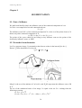
1.2.2. Grid, neighborhood graph
A graph is defined by a set of points which are called the vertices of the graph, and a set of
pairs of points taken among the vertices and called the edges of the graph.
A 2-D grid is a graph:
- whose vertices belong to Π2
- which is invariant under translation in Π2
- and where the segments joining every edge extremity cannot cross each other.
Apart from a few exceptions, the exercises deal with the hexagonal grid (this corresponds to
the default setup in MAMBA)..
1.2.3. Complementation
1.2.3.1. Binary images
c
X is the complementary set of X. Any point x which is not included in X belongs to Xc.
1.2.3.2. Greytone images
Image complementation is defined by:
fc = MAX - f
where f is the original image and MAX is the maximum grey level that can be used according
to the MAMBA image depth (256 for 8-bit images, 2 32 for 32-bit images).
1.2.4. Union, intersection
1.2.4.1. Binary images
X∪Y represents the union of the two sets X and Y, that is the set of all the points that belongs
to X or to Y. X∩Y represents the intersection of the two sets X and Y, that is the set of all the
points that both belong to X and Y.
5
© 2014, Serge Beucher
1.2.4.2. Greytone images, Sup, inf
Sup(f,g), also denoted f∨g, designates the sup of two functions f and g: for every point x,
(f∨g)(x) is the higher of the two values f(x) and g(x). Inf(f,g), also denoted f∧g, designates the
inf of two functions f and g: for every point x, (f∧g)(x) is the smaller of the two values f(x)
and g(x).
1.3. Some relations
1.3.1. De Morgan's formulae
These formulae express the duality of union and intersection:
(X ∪ Y)c = Xc ∩ Yc and (X ∩ Y)c = Xc ∪ Yc
Similarly:
(f ∨ g)c = fc ∧ gc and (f ∧ g)c = f c ∨ gc
1.3.2. Difference, symmetrical difference
X\Y denotes the set difference of X and Y. It is the set of those points belonging to X and not
to Y.
X\Y = X ∩ Yc
X*Y denotes the symmetrical set difference. It is the set of the points that belong to one and
only one of the two sets X and Y.
X*Y = (X ∩ Yc ) ∪ (Y ∩ Xc ) = (X ∪ Y)\(X ∩ Y)
1.3.3 Commutativity, associativity, distributivity
Union, symmetrical difference and intersection are commutative and associative operations.
The same properties apply to sup and inf.
commutativity:
X4Y=Y4X
f-g=g-f
(X 4 Y ) 4 Z = X 4 (Y 4 Z ) = X 4 Y 4 Z
associativity :
(f - g ) - h = f - (g - h )
Union and intersection are mutually distributive:
(X 4 Y ) 3 Z = (X 3 Z ) 4 (Y 3 Z )
(X 3 Y ) 4 Z = (X 4 Z ) 3 (Y 4 Z )
and so are sup and inf:
(f - g ) . h = (f . h ) - (g . h )
(f . g ) - h = (f - h ) . (g - h )
1.4. Other definitions
You will find below a quick reminder of some definitions which will be useful all along the
exercises.
1.4.1. Increasing transformations
A transformation ☞ is said to be increasing if it satisfies:
X _ Y e ☞(X ) _ ☞(Y )
f [ g e ☞(f ) _ ☞(g )
1.4.2. Extensivity
☞ is extensive if:
X _ ☞(X ) or f [ ☞(f )
6
© 2014, Serge Beucher
1.4.3. Idempotence
☞ is idempotent if:
☞[☞(X )] = ☞(X ) or ☞[☞(f )] = ☞(f )
1.4.4. Duality by complementation
✂ and ☞are both dual transformations if:
c c
c
✂(X ) = [☞(X c )] or ✂(f ) = [☞(f ) ]
EXERCISES
Exercise n° 1
This exercise aims at getting familiar with the MAMBA library. Perform the following
operations:
- Load images into memory (use the various ways available in MAMBA to do this).
- Display images, change the display palettes, use the superposer, etc.
- Save images.
- Get image information (size, depth, etc.).
- Use the interactive thresholder tool.
To achieve this, use the following MAMBA operators: load, showDisplay, hideDisplay,
save, setPalette, Superpose. Use also the imageMb constructor and its corresponding
methods: getSize, getDepth.
For this exercise and for the following, you can use the images which are provided in the
Images_Mamba directory. Five sub-directories are available: bin contains binary images,
grey contains greyscale images (8-bit), color (self explanatory), 32bit contains 32-bit images
and 3D contains few 3D images. Once copied on your disk, you are adviced to define the
Python working directory as such:
import os
os.chdir(“c:/Images_Mamba”)
to avoid long and boring path entries while manipulating these images.
Exercise n° 2
Prove that the function operators inf and sup can be expressed as set operations on
sub-graphs. (Prove in particular that the intersection of the sub-graphs f and g is the sub-graph
of the inf of f and of g).
Verify this with MAMBA (take two grey scale images and use the threshold and logic
operators).
Exercise n° 3
1) Prove and verify the De Morgan's formulae.
2) A transformation ☞ is defined as follows:
☞(X ) = X 4 Y , Y fixed set
- Is this transformation increasing, extensive, idempotent?
- Does there exist a dual transformation, and if so, indicate it.
3) Practice the corresponding MAMBA operators (logic, diff).
7
© 2014, Serge Beucher
Exercise n° 4
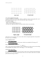
On the hexagonal grid each point has six neighbors. Translations are easily defined on this
grid.
Each translation is composed of elementary ones, e.g.:
t = t1 ) t1 ) t2 ) t2 ) t2
The set of translations equipped with the composition law constitutes the group of
displacements.
Practice the different shift operators available in MAMBA (shift, shiftVector). Do these
operators satisfy this group structure? Verify and explain your answer. (This phenomenon is
the first occurrence of the edge effects resulting from the fact that we work on a finite field of
analysis).
As a reminder, edge effects are due to the fact that, by default, MAMBA assumes that pixels
liable to fall outside the field are lost. When re-entering these pixels (by means of a
translation in another direction), they are given an arbitrary value. This behavior will have
important consequences for the definition of geodesic transforms, but also for classical
euclidean transforms. This will clearly appear in the following exercises.
8
© 2014, Serge Beucher
Chapter 2
EROSIONS & DILATIONS
2.1. Erosions, dilations, reminder
2.1.1. Binary case
The dilation of a set X by a set B of center O called a structuring element is a set Y thus
defined:
Y = X / B = x : Bx 3 X = π
→
where B x = x + Ob, b c B .
(X / B ) can also be written:
X / B = 4 X →
bcB
Ob
B is the transposed set of B (i. e. the symmetrical set of B with respect to O). The dilated set
Y is then the union of the translates of X.
Similarly, the eroded set is defined by:
Z = X 0 B = x : Bx _ X
which is also written:
X 0 B = 3 X →
bcB
Ob
These two transformations have the following properties:
(X 4 Y ) / B = (X / B ) 4 (Y / B )
(X 3 Y ) 0 B = (X 0 B ) 3 (Y 0 B )
(X / B 1 ) / B 2 = X / (B 1 / B 2 )
(X 0 B 1 ) 0 B 2 = X 0 (B 1 / B 2 )
which hold, whichever are the centers of B, B1 et B2 .
(1)
2.1.2. Greytone case
The sub-graph U(f) of a function f can be eroded and dilated by a three-dimensional
structuring element B and it can be shown, under certain conditions, that the dilation (resp.
the erosion) of a sub-graph is still the sub-graph of a function, called the dilation (resp. the
erosion) of f by B and denoted f / B (resp. f 0 B ).
If the structuring elements are planar, the dilation of a function f can be written:
→
(f / B )(x ) = sup f x + Ob
bcB
or else:
f / B = sup f →
bcB
Ob
→
where f → is the translated function of f of vector Ob.
Ob
Similarly, the erosion is defined by:
→
(f 0 B )(x ) = inf f x + Ob
bcB
or else:
→
f 0 B = inf f
bcB Ob
The relations (1) are immediately transposable to functions.
9
© 2014, Serge Beucher
(f - g ) / B = (f / B ) - (g / B )
(f . g ) 0 B = (f 0 B ) . (g 0 B )
(f / B 1 ) / B 2 = f / (B 1 / B 2 )
(f 0 B 1 ) 0 B 2 = f 0 (B 1 / B 2 )
(1')
EXERCISES
Exercise n° 1
1) Prove relations (1) and (1').
2) Prove or invalidate the following statements:
- Erosion and dilation are increasing,
- extensive, anti-extensive,
- idempotent,
- dual.
Exercise n° 2
1) Use the MAMBA operators (linearErode, linearDilate, doublePointErode,
doublePointDilate) to perform the following transformations:
- erosion and dilation by a segment of size n (consisting of n+1 consecutive points) in both
binary and greytone cases.
X 0 Ln, X / Ln, f 0 Ln, f / Ln
- erosion and dilation by a pair of points at a distance n:
X 0 Kn, X / Kn, f 0 Kn, f / Kn
(the origin of the two structuring elements is arbitrarily chosen at one extremity)
2) Prove that:
X 0 Ln _ X 0 Kn
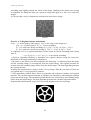
cat
objects
salt
shape
circuit
10
© 2014, Serge Beucher
Exercise n° 3
1) Prove that an elementary hexagon may be generated by three successive dilations of a point
by three judiciously chosen segments. Then, deduce an algorithm that allows to obtain the
erosion and the dilation by an hexagon. Program these transformations (both for the
hexagonal and square grids), and verify your algorithms on binary and greytone images.
2) Verify the duality of these transformations. Is the result satisfactory?
In the hexagonal case, the erosion and the dilation are not correct when the transformations
are made using only three directions. Therefore, it is necessary, in order to obtain unbiased
transformations at the edges, to perform the hexagonal erosion and dilation by means of
translations in the six main directions of the grid.
Exercise n° 4
1) Perform erosions and dilations on binary and greyscale images (use the erode and dilate
operators).
2) Which structuring element is used?
3) Modify the structuring element. Use a square one.
4) Can you explain the behavior of these operators at the edge of the images? Change the
edge parameter and see what happens.
You will see, in this exercise, that binary or greytone erosions produce a dark border when
you change the edge parameter to EMPTY. In this mode, the outside of the image is
considered as being empty. The objects under study are entirely included in the field of
analysis. However, this mode is penalizing, especially for greytone images because it deeply
reduces the image field when the size of the transformation increases. Therefore, when setting
the edge to FILLED, the structuring element B when crossing the boundary of the image
field D does not take into account its points which are outside D. This is equivalent to
perform the transformation with the structuring element B 3 D .
Exercise n° 5
1) Program the erosion by an elementary triangle, pointing upwards (take the point for
origin).
2) Program also the erosion by a 2x2 square.
3) What happens when the transformation is iterated? (Perform (X 0 B ) 0 B ). Represent the
structuring element B' such that:
(X 0 B ) 0 B = X 0 B ∏
A simple way to know how it looks is to dilate a point by B, twice. Indeed:
-
. / B / B = B / B =B / B
(X 0 B ) 0 B = X 0 (B / B ) e B ∏ = B / B
4) Program the dilation by a triangle pointing downwards.
5) Perform the dilations by the following structuring elements:
11
© 2014, Serge Beucher
If H is the elementary hexagon, find the structuring element which is equivalent to:
B1 / H / B2
In this exercise, the class structuringElement will be useful to define some of the proposed
structuring elements. Note also that some of them already exist in MAMBA: TRIANGLE,
SQUARE2x2, TRIPOD, etc.
Exercise n° 6
1) Use the dilations and erosions by dodecagons and octogons (dodecagonalErode,
dodecagonalDilate, octogonalErode, octogonalDilate). Can you explain how these
operations are performed (see previous exercise)?
2) Use large structuring elements (size > 100) and compare the speed of the previous
operators with the speed of the largeDodecagonalDilate and largeOctogonalDilate
transforms. Which kind of difficulty must be overcome when programming these large
structuring elements?
Exercise n° 7: Distance function
Let d be a distance defined on the points of the euclidean grid (length of the shortest path
drawn on the grid between two points). At any point x of X, the value of the distance function
is dist(x ) = d(x, X c ) = minc d(x, y ) .
ycX
Prove that if d is the distance defined on the hexagonal grid as the length of the shortest path
drawn on the grid between two points, the distance function can be obtained by means of the
successive erosions of X by a hexagon.
To do this,use the computeDistance operator and compare successive thresholds of the
obtained distance function with the corresponding erosions of increasing sizes.
12
© 2014, Serge Beucher
Chapter 3
MEASURES
3.1. Reminder
Any morphological transformation is to lead eventually to a measure on the
transformed set. The main function of a transformation (or sequence of transformations) is to
detect the objects to be measured: the openings revealing size distributions are an example.
Measures that satisfy good compatibility properties with translations and homothetics are not
so numerous. Namely:
- area
- diameter variations
- perimeter
- connectivity number
3.2. Measures and morphological transformations
Any measurement consists of two steps: transformation + counting of the points of the
transformed image. Measuring an area is very simple as the transformation is identity, it then
amounts to counting the points of the set. Besides, this measure is obtained when applying the
computeVolume MAMBA operator on any binary image.
In digitized images, the intercept numbers correspond to diameter variations:
1
1
I 1 = N(0 1) ; I 2 = N
; I3 = N
0
0
The transformation associated with this measure then consists in extracting the intercepts.
Measuring the connectivity number is a little more complex, since it requires double
transformations and counting:
0
0
0
✚=N
−N
1
1
1
Remind that in the plane, the connectivity number is considered as the number of connected
components minus the number of holes.
Programming measures is not enough, you have to learn how to interpret the results. Some of
the following exercises are intended to familiarize you with this important step of
morphological treatments.
EXERCISES
Exercise n° 1
The area of a binary image can be obtained with the computeVolume operator which also
provides the volume of a greytone image (8-bit and 32-bit).
1) Program the measurement of the intercept numbers (diameters) in the various directions of
the hexagonal grid.
13
© 2014, Serge Beucher
2) Program the measurement of the connectivity number. Test your algorithms on the holes
and cells images.
3) Program the measurement of the perimeter. Indicate several ways of obtaining this measure
and compare their respective accuracy.
holes
cells
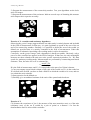
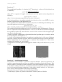
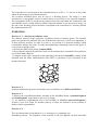
Exercise n° 2: transitive and stationary hypotheses
Observing the grains1 image suggests that the set under study is entirely known and included
in the field of measurement. In that case, it is quite legitimate to speak of the area of the set
and of its connectivity number. Similarly, it is possible to define the area of the eroded (or
dilated) set provided that it is entirely contained in the field of measurement. Under this
assumption of exhaustive knowledge, the working mode is said to be transitive.
Conversely, on the grains2 image, such a hypothesis is hardly acceptable. Obviously, only a
part of a more extended set appears in the field of analysis. In that case, the only meaningful
measures are those related to the unit area: ratio, specific connectivity number, etc. . We then
speak of a stationary working mode. Measurements are performed by constructing non biased
estimates. Thus, the ratio of a set X is estimated by:
mes(X 3 D )
t=
mes(D )
D is the field of measurement, and X 3 D corresponds to the part of set X that is known.
1) Can you compute a non biased estimate of the ratio of the eroded set X? (As the eroded set
X is biased in the field D, you have to find a field D' in which the eroded set is exact, and use
it to obtain the ratio estimate).
2) Same question for the dilated set.
3) Similarly, give an unbiased estimate of the ratio of the opened and closed sets.
grains1
grains2
Exercise n° 3
C(l) denotes the covariance of size l, the measure of the area (transitive case) or of the ratio
(stationary case) of the set X eroded by a pair of points at a distance l. In fact the
transformation itself is often called covariance.
14
© 2014, Serge Beucher
In the stationary case, the covariance is an estimate of the probability for a pair of points to be
included into the set X assumed to extend to the whole space.
1) Program the covariance. To do so, refer to the suggestions made below. (Especially, as
concerns the plotting of the curve).
2) Interpret the main features of the curve C(l), more particularly C(0), C(∞), tangent at the
origin, and overall outlook of the curve.
3) Application to particle1, particle2 and eutectic images.
eutectic
particle1
15
particle2
© 2014, Serge Beucher
Chapter 4
OPENINGS, CLOSINGS
4.1. Openings, closings, definitions
4.1.1. Binary case
Erosion and dilation lead to the definition of two new transformations, the opening γ and the
closing ϕ:
✏(X ) = (X 0 B ) / B
✩(X ) = (X / B ) 0 B
4.1.2. Greytone case
The opening and the closing are defined similarly:
✏(f ) = (f 0 B ) / B
✩(f ) = (f / B ) 0 B
4.1.3. Properties, size distribution
The opening is an increasing and anti-extensive operation. The closing is increasing and
extensive. The two transformations are idempotent.
If λB denotes the homothetic set of a convex set B, the opening is a size distribution. In
particular:
if ✘ > ✙, [(X ) ✘B ] ✙B = (X ) ✙B ✘B = (X ) ✘B
[(f ) ✘B ] ✙B = (f ) ✙B
= (f ) ✘B
✘B
The opening and the closing are used for size distribution analysis on the one hand, and for
filtering on the other hand. These two kinds of use are illustrated in the exercises.
EXERCISES
Exercise n° 1
1) In order to program the following transformations, use the ones (erosions, dilations)
already generated in the dictionary:
- opening and closing by a hexagon of size n,
- opening and closing by a segment of size n and
- opening and closing by a pair of points at a distance n.
2) Compare your results with the MAMBA operators (open, close).
3) Verify the properties stated above. Prove in particular the duality of opening and closing.
Verify also that the opening by a pair of points is not a size distribution (openings of small
size suppress more points than openings of greater size).
Exercise n° 2
The purpose of this exercise is to get you used to the behavior of opening and closing. So,
feel free to use the transformations introduced in the previous exercise and apply them to
16
© 2014, Serge Beucher
the provided images (grains1, grains2, particle1, particle2, balls, metal1, metal2, salt,
knitting, muscle). To help you in your quest, here are some guidelines.
balls
metal1
metal2
1) Verify the behavior of the opening as a size distribution, by applying transformations of
increasing size to the images grains2, balls, salt, knitting, muscle.
2) The notion of size distribution (or granulometry) is not related to the notion of particle.
Closings allow to perform (by duality) the size distribution of pores, and thus to reveal the
spatial distribution of the connected components of a set (images particle2, salt, knitting,
muscle).
3) Both opening and closing "sieve" the connected components of a set according to their
size, but also according to their shape. You can observe this by performing hexagonal
openings of increasing size on the image balls. Besides, opening "hexagonalizes" the
remaining connected components.
Note this selective effect on a greytone image by performing openings by segments of
increasing size (images circuit and burner).
muscle
burner
noise
electrop
Exercise n° 3
Opening and closing are good transformations for filtering noise in images. The noise image
represents a set blurred by a scatter plot and the electrop image represents a blurred greytone
image.
17
© 2014, Serge Beucher
1) Open the image with an elementary hexagon. Do the same with closing.
2) Perform the two operations successively. Does the order matter?
3) Can you enhance the filtering? (use triangular or 2x2 square openings and closings).
Exercise n° 4 : Generalization of the notion of opening
The notion of opening can be defined in a more general way. An algebraic opening is any
transformation that is:
- increasing
- idempotent
- anti-extensive
The notion of closing is defined by duality: increasing, idempotent and extensive.
1) Give some examples of openings and closings.
2) Is the operation consisting in extracting particles with at least one hole an opening? (binary
case)
3) To obtain new openings or closings, consider a family (γi) of openings or (ϕι.) of closings.
Prove that:
✏ = sup ✏ i resp. ✏ = 4 ✏ i is an opening.
i
i
i
i
✩ = inf ✩ i resp. ✩ = 3 ✩ i is a closing.
SupOpen is the MAMBA operator which performs the supremum of openings by segments
in the three directions of the grid and infClose is the corresponding closing.
4) Observe on the CIRCUIT and TOOLS images that the new openings and closings have a
different selective effect compared with those described up to now. We shall see further
(chapter 6) how to construct other openings acting still differently.
5) How to compute the area opening of a binary set?
Exercise n° 5
F(λ) denotes the ratio of the opening of size λ of a set X.
1) Verify that:
F(0 ) − F(✘ )
G(✘ ) =
F(0 )
is always comprised between 0 and 1. Compute it according to the area of the opened set and
to the area of the eroded field of measurement D' (D ∏ = D 0 2✘H).
2) Program this measurement. Application to the size distribution of the metal1 and metal2
images.
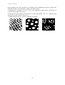
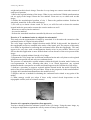
Exercise n° 6: analysis of the distribution of boron fiber
This study illustrates the judicious use of measures for solving a problem of quality control.
boron1
boron2
18
© 2014, Serge Beucher
The boron1 and boron2 images represent boron fibers in a composite material. These fibers
reinforce the mechanical resistance of the material. The resistance increases in proportion of
the regularity of the fibers layout. Therefore, during industrial production, they are as far as
possible placed according to a regular hexagonal network. However, irregularities occur.
The problem consists in quantifying these irregularities by means of an appropriate measurement. The image provided is already thresholded.
1) Simplify the images in filling up the fibers (this is not easy at all!). The fibers that cut the
field border are also to be filled.
2) Perform hexagonal closings of increasing size and observe the result. Propose an elementary measure to quantify the connections between the fibers?
3) Compute the theoretical value of the specific connectivity number according to the size of
the closing, in the case of a regular distribution. Derive a quantifier of the irregularity of the
structure.
19
© 2014, Serge Beucher
Chapter 5
MORPHOLOGICAL FILTERS
5.1. Reminder
Before we can extract any object from a greytone image, it is often necessary to
enhance the image. The enhancement of an image is mainly obtained by a filtering operation.
A morphological filter is a transformation φ which has the two following properties:
(i) φ is increasing
(ii) φ is idempotent.
5.1.1. Sequential alternate filter
The white (resp. black) alternate sequential filter (ASF) consists, as the name indicates, in
alternating morphological openings and closings (resp. closings and openings) of increasing
size. Let γn be a size distribution and ϕn an anti-size distribution, the white alternate sequential
filter of size n of a function f is defined by:
★ n (f ) = ✩ n ✏ n ✩ n−1 ✏ n−1 ...✩ 2 ✏ 2 ✩ 1 ✏ 1 (f )
Similarly, the black alternating sequential filter of size n of f is defined by:
✫ n (f ) = ✏ n ✩ n ✏ n−1 ✩ n−1 ...✏ 2 ✩ 2 ✏ 1 ✩ 1 (f )
5.1.2. Morphological center
4.1.2.1. Definition
Let (Ψi ) be a family of increasing transformations. Put:
✔ = .☞ i et ✓ = -☞ i
The center c of the family (Ψi ) is:
c = (I - ✔ ) . ✓
(I represents the identity function).
The center is not a filter (it is not idempotent), but it is convergent when iterated and its limit
is a filter.
4.1.2.2. Examples
1. for (Ψi ) = (γϕ, ϕγ) :
c(f ) = [f - (✏✩(f ) . ✩✏(f ))] . (✏✩(f ) - ✩✏(f ))
2. for (Ψi ) = (γϕγ, ϕγϕ) :
c(f ) = [f - (✏✩✏(f ) . ✩✏✩(f ))] . (✏✩✏(f ) - ✩✏✩(f ))
This center is also called an automedian filter (its limit being a filter).
5.2. Contrasts, Reminder
Let η be an anti-extensive transformation and ξ an extensive transformation of a function f. A
three-state contrast of primitives η and ξ is any transformation κ such that, for any f:
(i) κ(f)(x) only depends on ξ(f)(x), η(f)(x) and f(x) and on possible constants.
(ii) κ(f)(x) can only take one of these three values (the choice depending on a decision
rule).
Besides, if κ(f)(x) cannot take the value f(x), the contrast is said to be a two-state contrast.
20
© 2014, Serge Beucher
EXERCISES
Exercise n° 1
1) Without knowing it, you have already performed a sequential alternate filter (chapter 4,
exercise n° 3) on the noise image by means of hexagonal and triangular openings and
closings.
Continue this exercise:
- by increasing the number of iterations (size of the filter).
- by using different sizes of openings and closings (for example : a size of closing twice that
of the opening).
2) Program the sequential alternating filters for greytone images by using the various
openings and closings described up to now (hexagonal, dodecagonal, triangular, by sup of
linear openings).
Test them on the retina3, burner and electrop images.
retina3
Exercise n° 2
Let κ be the contrast of primitives ξ and η and its decision rule the following:
if ξ(f)(x) - f(x) ≤ f(x) - η(f)(x)
then κ(f)(x) = ξ(f)(x) if not ξ(f)(x) = η(f)(x)
1) How many states is the contrast κ?
2) Program κ:
a) for η = erosion of size N and ξ = dilation of size N.
b) for η = morphological opening of size N and ξ = morphological closing of size N.
c) for η = opening of size N and ξ = closing of size 5*N.
Apply these transformations to the chromosomes image.
3) Verify that the contrast defined in 2-a is not idempotent and that the one defined in 2-b is
idempotent.
chromosomes
21
© 2014, Serge Beucher
Exercise n° 3
Let κ' be a transformation defined by:
κ'(f) = 3f - γ(f) -ϕ(f)
(γ is an opening, ϕ is a closing).
1) Is κ' a contrast in the sense given above?
2) Program κ' and apply it to the chromosomes image.
Exercise n° 4
1) Program the automedian filter (which is not a filter according to the definition given
above) and apply it to the retina3 and burner images.
2) How many iterations are required for less than 10 % pixels to be modified? Try with
different sizes.
22
© 2014, Serge Beucher
Chapter 6
GEODESY
6.1. Reminder, binary case
Given a set X, the geodesic distance between two points x and y of X is defined as the length
of the shortest path L(x,y) included in X and joining these two points. We can now define
balls of size λ in this metric system, and then the erosion and dilation of a set Y included in X
by a geodesic ball B .
When one works on digitized sets, it can be shown that the elementary geodesic dilation is
defined by:
D X (Y ) = (Y / H ) 3 X
Similarly, the elementary geodesic erosion is defined by:
E X (Y ) = X 3 [(Y 4 X c ) 0 H ]
H being an elementary digital ball (hexagon or square).
6.2. Greytone case
In the greytone case, the geodesic space under consideration may be either a set X or a
function g (the latter case is the immediate generalization of the binary notion applied to
sub-graphs). On digitized sets, the following definitions apply:
The geodesic dilation of f into the set X by an elementary hexagon centered in O is defined at
any point x by:
→
sup
D X (f )(x ) =
f x + Ob = sup f(x ); x c H x 3 X
bcH
→
x + Ob c X
Likewise the erosion:
→
E X (f )(x ) =
inf
f x + Ob = inf f(x ); x c H x 3 X
bcH
→
x + Ob c X
The geodesic dilation of f conditionally to the function g by an elementary hexagon centered
in O is defined by:
D g (f ) = inf(f / H, g )
Likewise the erosion:
E g (f ) = sup(f 0 H, g )
NB : Note that the duality is different from the one defined in the binary case. Here we simply
replace f by m-f (where m=255 for 8 bits images).
23
© 2014, Serge Beucher
EXERCISES
Exercise n° 1 : Geodesic reconstructions
The build, dualBuild, hierarBuild, hierarDualBuild operators, which implement
reconstructions of a function f with a function g as marker are already efficiently installed
(with different algorithms) in MAMBA.
1) Let X be a set composed of several connected components {Xi ). A set Y included in X
marks one or several connected components of X. Reconstruct the connected components of
X marked by Y (these connected components consist of points x of X which are at a finite
geodesic distance d(x,Y) from Y).
2) Test this reconstruction on the tools image by using as a marker an image entirely set to 0
except in a point (selected preferably at the location of an object) where the value is set to
255.
3) Do the same operation on the retina1 image, by placing the point on the blood lattice.
tools
retina1
retina2
Exercise n° 2: Opening by erosion - reconstruction
Prove that the reconstruction by geodesic dilation of the erosion of f (resp. X) of size n by the
structuring element B conditionally to f (resp. X) is an opening (the center of the structuring
element B must be a point of B).
Program these operations, as well as the dual closings and compare them on the retina1,
retina2 and cat images with the openings previously described.
Exercise n° 3: Individual analysis of particles
1) Design an algorithm allowing the individual analysis of particles, in other words capable of
extracting every connected component from an image in order to measure it.
2) Application to the measurement of the area of grains on the particle1 image.
3) Verify that the transformation ☞(X ) defined in this way:
n
X = 4 X i , Xi connected component of X
i=1
☞ ✘ (X ) = 4X j such that mes(X j ) > ✘
is a size distribution.
Exercise n° 4: Holes filling, objects cutting edges
1) Apply the geodesic reconstruction algorithm to suppressing the particles cutting the field
border. What can be in particular the marking set Y? Application to the grains2 image.
2) How can you fill the holes in the particles? Design an algorithm and test it on the holes and
gruyere images.
3) On a greytone image, a hole may correspond to what is called a basin if the image is
considered as a relief. We can then imagine to fill up these holes, as would rain water, the
24
© 2014, Serge Beucher
exceeding water spilling outside the limits of the image. Similarly to the binary case, design
an algorithm for filling the holes on a greytone image and apply it to the circuit and tools
images.
4) Can you find a way to eliminate the inclusions in the alumine image?
alumine
Exercise n° 5 :Regional maxima and minima
Let p0 ,...,pn be the points of the image I. V(pi ) is the value of the image in pi .
p0 p1 ...pn is called a path if, ∀i, pi+1 et pi are neighbors.
p0 ...pn is said to be strictly ascending if, ∀i, V(pi+1 ) ≥ V(pi ) et V(p0 ) < V(pn ).
p0 ...pn is said to be strictly descending if, V(pi+1 ) ≤ V(pi ) et V(p0 ) > V(pn )
A connected set X is a regional maximum if there exists no strictly ascending path coming
from X:
≤x c X, ≤(p i ) ic…1...N c I N , xp 0 ...p N is not strictly ascending.
1) Find an algorithm allowing to determine the regional maxima using the successive
thresholds of the image and binary reconstruction.
2) In practice, one does not use this method but the following: 1 is subtracted from the image
and the resulting image is reconstructed from the initial image. The regional maxima are
located where the resulting image differs from the initial image. The dual algorithm generates
the regional minima.
Program this transformation. Apply it to the electrop image. What do you observe? How can
you explain this? Can you propose a solution?
3) The algorithmic method above allows to generalize the notions of minima and regional
maxima. The extended regional maxima at a height h are obtained by subtracting the constant
h from the initial image. The extended regional maxima are located where the resulting image
differs from the initial image. The dual algorithm generates the extended regional minima.
Program this transformation. Apply it for increasing heights to the electrop image.
wheel
25
© 2014, Serge Beucher
Exercise n° 6
This exercise shows how a very simple transformation (opening here) combined with geodesic reconstructions can solve a problem of detection and counting of the teeth of a notched
wheel when it is associated to a preliminary selection of the zone where these teeth should be.
Use image wheel to extract and count its teeth.
Exercise n° 7: size distribution of a greytone image
When a size distribution transformation is applied to a binary image, the computed size distribution curve (see chapter 4, exercise 5) may be considered as a texture index characterizing
the size of the particles (case of the opening by a disk), the size of the pores separating the
particles (closing by a disk) or else the main directions of the image (use of linear structuring
elements).
A particularity of the morphological notion of size distribution is that it can be applied to non
individualizable structures. The value which is then taken into account is, for example, the
subtracted or added area for each operation of increasing size. The size distribution is then
said to be "in measure" and is opposed to the size distribution in number which only applies
to isolated particles.
The greytone size distribution is also an "in measure" size distribution but here, the measure
more often bears on volumes than on areas. The size distribution curve will also be considered as a texture index but this time it characterizes a relief: shape, size, height of the volume
structures contained in the sub-graph of the image.
We will try to use a greytone size distribution in order to characterize the presence of nodules
(small white domes) on lung radiographs.
Let us recall the properties to be satisfied by a size distribution transformation.
Let X be the initial set (the sub-graph of an image in our case). Let T be the sieving transformation applied to this set. We denote T(X) the part of X which has been retained by the sieve
of size 1. If T fulfills the three following rules, it may be considered as a transformation with
good size distribution qualities:
1. The operation must be anti-extensive, in other words the part retained by the sieve must be
a sub-set of X.
2. The operation must be increasing.
3. The operation must satisfy the following size criterion:
Tl1(Tl2(X)) = Tl2(Tl1(X)) = Tsup(l1,l2)(X) ∀ l1, l2 > 0
We know that the opening satisfies the three properties.
lung1
lung2
The images to be studied are lung1 and lung2. lung1 represents a sound lung, lung2 a lung
with a nodular texture. The nodules are small white "clouds" distributed on the whole image.
1) Which kind of greytone transformation satisfying size distribution rules would allow to
reveal the difference in texture between the two lung images?
26
© 2014, Serge Beucher
- Program a size distribution function from this transformation.
- Does it effectively differentiate the two images?
- What do we learn from the position of the maximum of the size distribution curve?
- and from the range of this maximum?
2) What can be the use of a greytone opening by reconstruction? Program the size distribution based on openings by reconstruction and try to explain the differences between the two
types of size distribution curves.
3) Indicate the third type of opening that can be used as a basic size distribution function to
analyze these images? Why is the range of this curve much lower than the preceding?
4) Is it possible to apply a size distribution in number to a greytone image?
27
© 2014, Serge Beucher
Chapter 7
RESIDUES I
The following exercises introduce morphological transformations which belong to the
class of residual operators. Among them, the gradient and top-hat operators are rather simple
(they use simple primitives). Other operators use families of primitives. In this chapter,
residues using erosions and openings will be addressed. The next chapter will be devoted to
residues based on the Hit-or-Miss Transform (HMT).
7.1. Gradients
7.1.1. Classical gradient
The gradient of a function f defined on ‘ 2 is defined as the vector:
Øf
Øx
∫f = Øf
Øy
In the digital case, the first-order differences may be used to express the partial derivatives:
(∫ x f )(x, y ) l f(x, y ) − f(x − 1, y )
(∫ y f )(x, y ) l f(x, y ) − f(x, y − 1 )
1
Digital convolutions of f are recognized by the kernels [-1 1] and
.
−1
We could also use the following differences as the expression of the partial derivatives:
(∫ 2x f )(x, y ) l f(x + 1, y ) − f(x − 1, y )
(∫ 2y f )(x, y ) l f(x, y + 1 ) − f(x, y − 1 )
They have the advantage of being centered in (x,y). These derivatives are performed with the
1
digital convolutions of f by the kernels [-1 0 1] and 0 .
−1
In practice, other differences are also used, which may be expressed in terms of digital
convolutions too. An abundant literature illustrates this subject. For example, the Sobel
operator is given for the following convolutions:
−1 0 1
1 2 1
1
1
−2
0
2
0
0 0
and
4
4
−1 0 1
−1 0 −1
7.1.2. Morphological gradient
The morphological gradient of a function f defined on ‘ 2 or on a sub-set is given by:
(f / ✘B ) − (f 0 ✘B )
g(f ) = lim
✘d0
2✘
where λB denotes a ball of radius λ.
On a hexagonal grid, we get:
(f / H ) − (f 0 H )
g(f ) =
2
28
© 2014, Serge Beucher
where H is a hexagon of size 1. This gradient is equal to the gradient module of a function f
continuously derivable.
7.2. Top-hat
The top-hat is a transformation that only applies to greytone images. The top-hat WTH of a
function f is defined by:
WTH(f) = f - γ(f) (white Tophat)
Likewise, the conjugated top-hat BTH of a function f is defined by:
BTH(f) = ϕ(f) - f (black Tophat)
EXERCISES
Exercise n° 1
1) On the road image, apply the morphological gradient of size λ of a function f:
g(f ) = (f / ✘B ) − (f 0 ✘B )
where λB denotes a ball of size λ (take here B = H).
2) Program the top-hat WTH(f) associated with the opening by a hexagon of size n and the
conjugated top-hat BTH(f).
3) Apply these transformations to the circuit, electrop, grains3, retina1 and retina2 images.
4) Note that these operations do not permit the discrimination of the aneurysm vessels (small
white spots) on the images retina1 and retina2 images. Find a top-hat allowing such
discrimination.
road
grains3
Exercise n° 2: Ultimate erosion of a (binary) set
Let X be a set. The ultimate erosion of X is defined by:
U(X ) = 4
x c X 0 nH; d X0nH (x, X 0 (n + 1 )H ) = +∞
n
U(X) is then the set of the connected components resulting from the successive erosions of X
that cannot be reconstructed after the erosion of the immediately larger size.
1) Design the algorithm and program the ultimate erosion of a set X.
2) Apply it to the cells image. Compute the number of cells in the aggregate.
3) Try to determine the limits of this transformation as a tool for separating particles.
Exercise n° 3: Skeleton by maximal balls (binary case)
Let X be a set. A ball of radius λ included in X is said to be a maximal ball if and only if no
ball of a radius strictly larger and containing the ball of radius λ can be found in X.
Bλ maximal: Bλ ⊂ X; there exists no Bµ , µ > λ, Bλ ⊂ Bµ ⊂ X
29
© 2014, Serge Beucher
The locus of the centers of the maximal balls of X, S(X) is called the skeleton of X. When X
is defined on the hexagonal grid, the notion of maximal ball is replaced by that of maximal
hexagon. The purpose of this exercise is to define an algorithm which performs the skeleton
S(X) of X.
1) Let X 0 nH , be the erosion of size n of X. Prove that if x is a point of X 0 nH which does
not belong to the open set (X 0 nH ) H , this point is the center of a maximal hexagon of size n.
2) Derive the algorithm performing the skeleton S(X) of X.
3) To any point x of S(X), can be associated the radius r(x) of the maximal hexagon centered
in x. The function r(x) of support S(X) is called a quench function. Verify that the pair
(S(X),r(x)) suffices to reconstruct the set X:
X = 4 H(x, r(x ))
xcS(X )
4) Compare the skeleton of the set X with its ultimate erosion.
5) What are the drawbacks of this transformation in the digital case?
Exercise n° 4: Distance function and maxima
This exercise considers again the notion of distance function introduced in chapter 2 and the
corresponding procedure computeDistance.
1) Prove that the local maxima of the distance function are the points of the skeleton by
maximal balls. Illustrate it on the coffee image.
2) Prove that the regional maxima of the distance function are the ultimate eroded sets.
Observe it on the coffee image. What can be the interest of the extended regional maxima of
the distance function? Test it on the coffee image.
coffee
30
© 2014, Serge Beucher
Chapter 8
RESIDUES II
THINNINGS AND THICKENINGS
8.1. Introduction
The transformations developed in the following exercises are more sophisticated.
According to our previous comparison, they are the true "machine-tools" of MM. They are at
the meeting point of geodesy and homotopy. We have already handled geodesic
transformations, therefore we shall only recall the notion of homotopy, and especially that of
homotopic transformation.
8.2. Binary thinnings, reminder
Let T = (T1 ,T2 ) be a two-phase structuring element. The hit-or-miss transformation of a set X
by T is equal to:
X & T = (X 0 T 1 ) 3 (X c 0 T 2 )
The thickening of X by T is equal to:
X \ T = X ∪ (X * T)
and the thinning is defined by:
X 0 T = X\(X * T)
Thinning and thickening are both dual transformations:
(Xc \T)c = [Xc ∪ (Xc * T)]c = X ∩ (Xc * T)c = X \ (X * T') = X 0 T'
where T' = (T2 ,T1 ).
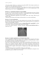
8.3. Homotopy
Two paths of a set X are homotopic if it is possible to superpose one another by a sequence of
continuous deformations. "Continuous" means without cut and that all intermediary paths are
included in X.
Homotopic paths on the hexagonal grid
31
© 2014, Serge Beucher
By extension, a transformation Ψ which preserves homotopy is said to be homotopic.
Intuitively, a homotopic transformation Y = Ψ(X) transforms the set X in a set Y that can be
superposed on X by a continuous deformation.
When the set X is digitized according to a (square or hexagonal) grid, matching paths is easy
since any path can be defined as the concatenation of elementary edges. A homotopic
transformation does not break any paths.
8.4. Greytone thinnings
Let m(x) = sup f(y )and M(x) = inf f(y ) .
ycT 2 x
ycT 1 x
The thickening of f by T = (T1 ,T2 ) is defined by :
(f \ T) (x) = M(x), iff m(x) ≤ f(x) < M(x)
(f \ T) (x) = f(x), if not.
The thinning of f by T = (T1 ,T2 ) is defined by:
(f ° T) (x) = m(x), iff m(x) < f(x) ≤ M(x)
(f ° T) (x) = f(x), if not.
EXERCISES
Exercise n° 1
On the hexagonal grid, the most interesting structuring elements, T = (T1,T2) are those defined
on the elementary hexagon:
T1 ⊂ H, T2 ⊂ H
We can even write: T 1 3 T 2 = π . Indeed, T1 and T2 must have no common point if we want
X*T to be different from an empty set.
1) Program the binary and greytone thickening and thinning by any structuring element
defined on the elementary hexagon. The hit-or-miss transformation imhitormiss is already
available.
2) Apply the algorithms to binary images. In particular, perform the following operations:
- delete the white and black isolated points in the noise image.
- contour a set in only one transformation.
Exercise n° 2: Geodesic thickenings and thinnings
Let X be a set included in Z. The geodesic thickening of X by a structuring element T
included in the elementary hexagon can be defined by:
(X \ T) = (X \ T) ∩ Z
1) Test this transformation (geodesicThick, fullGeodesicThick)..
2) Since thinning is the dual operation of thickening, geodesic thinning is defined by:
(X ° T) = Z/[(Z\X) \T']
Simplify and program this transformation (geodesicThin, fullGeodesicThin).
Exercise n° 3
1) Find all possible configurations (up to a rotation) for the neighboring of a point in the
hexagonal grid (they are 14).
32
© 2014, Serge Beucher
2) Prove that the relation of homotopy for two paths C1 and C2 with same origin and same
extremity included in a set X is a relation of equivalence.
3) From this, deduce which of these configurations generate a homotopic thinning.
Exercise n° 4
1) Program the connected skeleton by using the structuring elements L, M and D (thinL,
thinM, thinD). Compare the results.
2) Indicate the transformations allowing to extract the characteristic points of a skeleton:
- extremities
- n-uple points
- single points
L
M
D
3) The direction of rotation and the starting orientation of the structuring elements used for
the different skeletons are totally arbitrary. Consequently, more or less important variations
occur in the resulting skeleton. These variations may even generate artifacts.
Generate one of the two following images:
Apply to this image a skeleton of type L by thickening, and judge the result. Is it possible to
improve the algorithm?
Exercise n° 5
The exercise 3 has allowed you to define homotopic thinnings on an elementary hexagon.
1) Among the selected configurations, Study their effect on the length of the homotopic paths,
after thinning. Indicate in particular why the following configuration is special.
*
*
0
*
*
0
0
2) Deduce from this an algorithm for detecting the geodesic center of simply connected sets.
Program this algorithm.
Exercise n° 6
Program, by means of geodesic transformations, the geodesic skeleton by thickening. Verify
in particular that only the M structuring element allows to obtain a correct transformation.
33
© 2014, Serge Beucher
Exercice n° 7
The morphological gradient of a function f of ‘ 2 that takes its values on ‘ in the direction α
is defined by:
(f / ✘L ✍ ) − (f 0 ✘L ✍ )
g ✍ (f ) = lim
✘d0
2✘
where ✘L ✍ is a segment of length λ in the direction α. In the digital version, the gradient is
defined by:
g ✍ (f ) = (f / L ✍ ) − (f 0 L ✍ )
α
where L is the elementary segment in the direction α of the grid.
→
In the horizontal plane, the gradient azimuth is the direction of the vector grad(f ). It can be
defined in the directions of the digitization grid.
A new gradient can be defined in the direction α by means of thickenings and thinnings. The
directional gradient in the direction α is defined by:
g ✍ (f ) = (f ? T ✍ ) − (f ; T ✍ )
where T1 and T2 form the two-phase structuring element Tα = (T1 ,T2 )α .
The maximal directional gradient may occur in several directions simultaneously. Then, we
have to compute the most probable direction. To do so, we take into account that computing
these gradients implies that three directions at most can be extracted in the hexagonal grid
resp. four in the square grid.
1) Find all possible configurations of maximal directional gradients (up to a rotation, and in
the hexagonal grid). Their number is 5.
2) In case of non adjacent directions, the gradient is considered to be 0. In case of adjacent
directions, a unique direction is selected, which is the mean direction of all present directions.
Which configurations do we obtain (up to a rotation)? Their number is 3. What is the
resulting effect and how can it be avoided?
3) Program the directional gradient and apply the azimuth to the petrole and seismic_section
images.
petrole
seismic_section
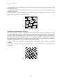
Exercise n° 7: classification of particles
This problem is not related to a particular study but underlies numerous applications. It
consists in separating particles or objects according to the number of holes they contain. This
kind of problem is particularly found in industrial vision (discrimination of objects according
to the number of their perforations), in automated character recognition (character classification), in bio-medical imagery (separation of cells with or without nucleus), etc. This separation is in fact a direct application of the notion of homotopy.
By means of the gruyere image, solve the following problems:
1) In the image, separate the particles without hole from the particles with holes.
34
© 2014, Serge Beucher
2) Among the particles with holes, separate those with one and only one hole from those with
more than one hole.
3) Among the particles with more than one hole, extract those with two holes only from those
with three and more.
4) Is it possible to design algorithms that separate objects according to the number of their
holes? Is this separation a size distribution?
gruyere
Exercise n°8: dislocations in eutectics
The eutectic image represents a lamellar eutectic material. This structure is characterized by a
two-phase lamination, with here and there undesirable defects characterized by discontinuous
lamellae. These discontinuities due to dislocations in the crystalline assembly of the material
jeopardize its mechanical properties. The loss in resistance depends, among other things, on
the length of these dislocations. You then have to find a sequence of operations for materializing these dislocations so as to be able to measure their length.
1) Try to detect the extremities of the lamellae (extremities of the skeleton or another
solution).
2) Try next to connect judiciously these extremities, so as to obtain an arc materializing each
dislocation.
eutectic
35
© 2014, Serge Beucher
Chapter 9
SEGMENTATION
9.1. Zone of influence
We shall recall briefly what is the influence zone of the connected component of a set.
Let X be a set composed of several connected sub-sets:
X = 4 Xi
i
The influence zone Z(Xi ) of the connected component Xi, is the set of the points closer to Xi
than to any other connected component of X.
x c Z(X i ) g d(x, X i ) < d(x, X j ), ≤j ! i
The points of the space which do not belong to any influence zone are the points of the
skeleton by influence zones, or SKIZ.
9.2. Watershed transformation
Let f be a greytone image. f is assumed to take discrete values in the interval [hmin,hmax].
Denote Th(f) the threshold of f at level h:
T h (f ) = p, f(p ) [ h
Watershed by flooding
Minh(f) is the set of the minima of f at level h, and IZA(B) represents the influence zone of B
in A.
The set of the catchment basins of an image f is equal to the set X h min resulting from the
following recursion:
(i) X h min = T h min (f )
(ii) ≤h c [h min , h max − 1 ], X h+1 = Min h+1 4 IZ T h+1 (f ) (X h )
36
© 2014, Serge Beucher
The watershed of f corresponds to the complementary set of X h max , i.e. the set of the points
which do not belong to any catchment basin.
The recursion described above may be seen as a flooding process. The image f is then
considered as a topographic surface in which holes are pierced in every regional minimum.
The topographic surface is progressively plunged into water and dams are constructed each
time that the waters coming from two distinct regional minima are on the point to merge. At
the end of the flooding process the dams correspond to the watershed of f, and they delimit
the catchment basins of f.
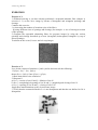
EXERCISES
Exercise n° 1 : Skeleton by influence zones
The (binary) alumine image represents a polished section of alumine grains. The metallic
grains are joined in the material. Since the joint thickness does not exceed a few angstroms, it
is then perfectly invisible. In order to reveal it, we proceed to a chemical etching, which
considerably enlarges the joints. To study the neighboring relationships between the grains, it
is necessary to thin the joints.
1) Perform the SKIZ of the grains (computeSKIZ)..
2) Prove that the skeleton by influence zones can be obtained by a watershed with a judicious
use of the distance function.
3) Compare on the coffee image the result obtained by this method (fastSKIZ) with the result
obtained with the direct transformation (The SKIZ is equivalent to the watershed of the
distance function).
alumine
Exercise n° 2
Program similarly the geodesic skeleton by zones of influence (use fullGeodesicThick)..
Exercise n° 3
1) Practice the watershed transforms available in the MAMBA library (watershedSegment
and basinSegment). Apply them to the electrop image.
2) An interactive segmentation tool is also available in MAMBA (interactiveSegment).
Practice it (on tools image for instance) and try to show the influence of the position of
markers on the segmentation.
Exercise n° 4
The two-dimensional electrophoresis is a technique for separating and
identifying proteins. The migration of the proteins on the gel depends on their molecular
37
© 2014, Serge Beucher
weight and on their electric charge. From the electrop image we want to extract the contour of
each spot of proteins.
1) Detect the regional minima of the image. What is your conclusion? Which transformations
can we apply to the image? Detect the new minima. From now on, we shall work on this
image.
2) Define the morphological gradient of size 1. Detect the gradient minima. Perform the
watershed transform. Is the result satisfactory?
3) We will try to obtain a better result. To do so, we will first seek to detect the markers
located inside the spots and to contour the exterior markers as well.
- What can we take as interior markers?
- As exterior markers?
- Perform the watershed transform controlled by this new set of markers.
Exercise n° 5: catchment basins in a digital elevation model
This study uses the segmentation of images by watershed. It is devoted to the extraction of the
catchment basins of a digital elevation model.
The relief image represents a digital elevation model (DEM). In this model, the altitudes of
the topographic surface are sampled at the nodes of the square grid. The purpose of this study
is to define an algorithm for extracting the catchment basins from the topography. This may
appear to be easy since such a transformation already exists in your toolbox. However you
will see that this application is more difficult than it seems because of the noise present in the
image.
1) Extract the regional minima from the relief image.
2) Segment the relief image into its different catchment basins and verify that to each regional
minimum corresponds one and only one catchment basin.
The presence of undesirable regional minima within the digital elevation model induces an
over-segmentation. In fact, assuming that there is no closed depression, any regional
minimum should correspond to an outlet and should appear on the field border of the image.
3) Indicate a procedure to suppress regional minima located inside the model. Display the
mask of the pixels modified by this procedure. What are the properties of this transformation?
4) Apply the watershed transformation to the modified relief.
5) Propose and test a method for obtaining the catchment basin related to any point of the
model.
6) What strategy would you adopt if there really existed closed depressions on the
topographic surface (such as volcanic craters)?
relief
Exercise n°6: separation of particles (first approach)
You have already defined the ultimate erosion of the cells image. Using the same image, try
to design an algorithm to segment the cells by means of binary operations only.
38
© 2014, Serge Beucher
1) Use the geodesic skeleton, or even better, the geodesic SKIZ of the ultimate eroded sets in
the initial set. Is the segmentation satisfactory?
2) How can you improve this segmentation? (by taking into account the order of the ultimate
eroded sets). Use again the watershed transform and use it on the complementary of the
distance function f(x) = d(x,Xc (computeDistance).
Exercise n° 7: separation of particles (second example)
The previous case-study showed how to program watershed segmentation by means of binary
operations only. It also presented an ideal case of segmentation which works immediately.
This is not always the case as will prove the next example.
1) Apply the segmentation algorithm seen previously on the coffee image. What can you
observe? Why?
2) Show how the filtering of the distance function allows to overcome this difficulty.
Exercise n° 8: road segmentation
The purpose of this exercise is to extract the roadway in the route image. This corresponds to
the first step of the road segmentation procedure used to initiate the process on a sequence of
images (see the MAMBA examples).
1) Use the hierarchical segmentation operators (enhancedWaterfalls, segmentByP) to define
a road marker. Generate an outside marker from the first marker.
2) Use the marker-controlled watershed transform (markerControlledWatershed) to
segment the road.
route
Exercise n° 9: pellets segmentation in a 3D polyurethane foam
This 3D segmentation example shows that a process which has been designed for 2D images
can be applied directly to 3D images thanks to the availability in mamba3D module of operators which are the simple transposition of 2D operators.
The initial 3D foam image represents a foam made of polyurethane pellets. However, these
pellets are so compressed that the separation walls between them have disappeared. Only
corners at the junction of adjacent pellets are still visible. Nevertheless, it is possible to
rebuild the separation walls with a procedure which is, in 3D, similar, indeed identical, to the
approach used to segment coffee grains in exampleA2.py (coffee grains separation and
counting).
1) Use the display operators in mamba3D to display yhe initial image.
2) Transpose in 3D the segmentation process defined for the coffee grains by using the corresponding 3D operators available in the 3D module.
39
© 2014, Serge Beucher
foam
Exercise 10: stamped grid on steel
A regular grid has been printed on a steel sheet before its stamping. This example shows how
the crossing points of this grid after stamping can be extracted. The new position of each
point indicates its displacement during stamping and therefore the degree of stress exerted
locally on the steel sheet.
1) Design a filtering procedure applied on the steel_sheet image to extract sufficiently good
markers of the grid cells (we suggest to use levellings filters. Don’t try to attain perfection,
multiple markers in a single cell are allowed).
2) Use the watershed operator to extract the grid.
3) Extact the crossing points of the grid.
steel_sheet
Exercise n° 11: analysis of a burner
The burner image represents a detail of a gas heating appliance. The infrared emitter consists
of:
- a ceramic plaque with cylindric holes opening onto the surface by cavities forming truncated
cones with a hexagonal base.
- a raster formed of longitudinal and transversal metallic wires.
From a morphological point of view, the interesting structures are the following:
- The raster which appears on the image under the form of linear horizontal and vertical
structures in light grey tone.
- The hexagonal structures a little darker.
- The black spots situated inside the hexagons. Both spots and hexagons may be partially
hidden by the raster.
- The background of the image present higher grey levels (white tone).
The purpose of this study is to extract a mask of the raster and to be able to place correctly
(with respect to the grid) the center of the spots.
1) What kind of grid is it interesting to use?
40
© 2014, Serge Beucher
2) Use morphological filters in order to reduce the granular aspect of the image without
modifying the structures of interest. Do you note a significant difference between the filters
based on closing-opening and those based on opening-closing?
3) Segment the raster by using only greytone transformations. Do we obtain an equivalent
result with binary operations? How can we solve this problem on a hexagonal grid?
4) Try to isolate the black spots by a morphological top-hat. Is the result satisfactory? How
can you explain that the spots close to the raster seem to be more contrasted than the others
when a top-hat of size 7 is used? How can you explain that a top-hat of size 14 produces the
opposite?
5) Find a transformation that detects the "valleys" on a depth criterion without taking the size
criterion into account?
6) Detect the centers of the black spots. Is there a way of detecting the spots whose centers are
hidden by the raster?
41