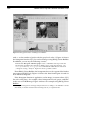
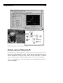
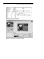
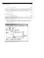
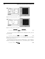
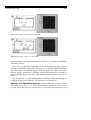
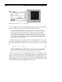
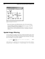
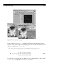
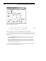
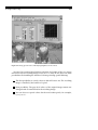
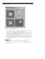
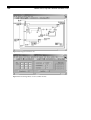
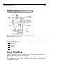
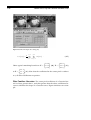
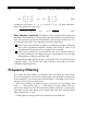
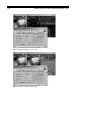
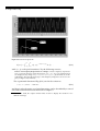
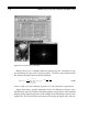
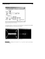
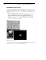
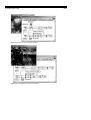
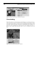
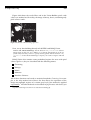
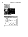
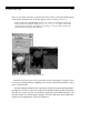
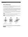
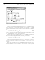
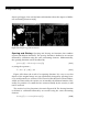
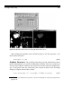
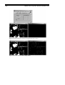
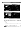
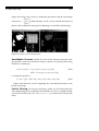
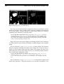
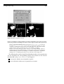
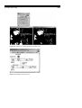
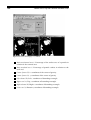
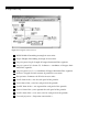
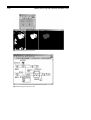
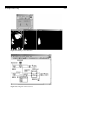
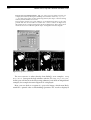
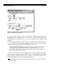
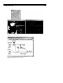
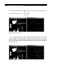
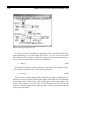
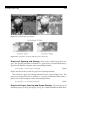
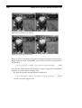
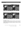
1
Our images have now found their way from the generation device over transport or storage media to the image processing and analysis software, in our case, IMAQ Vision. As defined in Chapter 1, the output of an image processing operation is still another image; this chapter, therefore, focuses on methods like image manipulation using look-up tables, filtering, morphology, and segmentation. Here and in Chapter 5, I tried to provide exercises and examples without any additional hardware and software. When that is not possible, I specify exactly the type of hardware equipment and where to get additional software. Moreover, I keep as close as possible to the IMAQ Vision User Manual [4], which means that I use the same symbols and equations but also give more information and examples. Gray-Scale Operations The easiest way, of course, to alter a digital image is to apply changes to its (usually 8-bit, from 0 to 255) gray-level values. Before we do this, it might be interesting to learn how the gray-level values of an image are distributed. Histogram and Histograph IMAQ Vision provides two simple tools for this distribution; they do almost the same thing: The histogram gives the numeric (quantitative) information about the distribution of the number of pixels per gray-level value. The histograph displays the histogram information in a waveform graph. According to [4], the histogram function H(k) is simply defined as H(k) = nk ; (4.1) 152 IMAGE Processing with LabVIEW and IMAQ Vision Figure 4.1. Histogram Function in IMAQ Vision Builder with nk as the number of pixels with the gray-level value k. Figure 4.1 shows the histogram function H(k) for our bear image using IMAQ Vision Builder. In addition, you can try the following exercise. Exercise 4.1: Histogram and Histograph. Create a LabVIEW VI that provides the functionality described above directly in IMAQ Vision, using the functions IMAQ Histogram and IMAQ Histograph. You can find them under Motion and Vision / Image Processing / Analysis.1 Figure 4.2 shows a possible solution. From IMAQ Vision Builder, the histogram data can be exported for further processing into MS Excel; Figure 4.3 shows the data from Figure 4.1 and 4.2 in an MS Excel diagram. If the histogram function is applied to a color image, it returns values H(k) for each color plane; for example, three histograms for red, green, and blue in the case of an RGB image. Figure 4.4 shows an example using IMAQ Vision Builder. 1 Actually, the histogram is an image analysis function according to our definition. On the other hand, we need its results for the following sections, so I explain it here. 4. Image Processing 153 Figure 4.2. Histogram and Histograph of an Image Using Look-up Tables (LuT) You know how to adjust brightness and contrast values of your TV set or TV video PC card; the intention is to get a “better” image, what obviously means a better distribution of the gray-level values. This is achieved by a function f (g) (g are the gray-level values), which assigns a new value to each pixel. If we consider Eq. (1.1), then our function f (g) will modify the gray-level values according to 154 IMAGE Processing with LabVIEW and IMAQ Vision Figure 4.3. Histogram Exported in MS Excel Figure 4.4. Color Histogram Function in IMAQ Vision Builder 155 4. Image Processing sout (x, y) = f (sin (x, y)) (4.2) , with sin as the original values and sout as the resulting values. Because the possible results are limited to 256 values, the function f (g) usually is realized by a table consisting of 256 values, a look-up table (LuT). Therefore, if LuT (g) = f (g) (4.3) , Eq. (4.2) will change to sout (x, y) = LuT (sin (x, y)) . (4.4) Special LuTs: Math Functions. The easiest way to generate a LuT is to use mathematic functions, such as logarithmic, exponential, and power. We try this in the following exercise. Exercise 4.2: Look-up Tables. In this and the following exercise we compare the fixed IMAQ Vision functions to the impact of manually generated LuTs. First of all, create the VI shown in Figure 4.5. Figure 4.5. Exercise 4.2: Creating User LuTs 156 IMAGE Processing with LabVIEW and IMAQ Vision Use the function IMAQ UserLookup to generate the second image, which is used for the comparison of the result to the built-in IMAQ function; here, the function IMAQ MathLookup. An XY graph displays the entire LuT by a simple line. Figure 4.6. Processing Look-up Tables (LuTs) Figure 4.6 shows the front panel of Exercise 4.2. Case 0 of the VI leaves the gray-level values of the original image unchanged, which means that the location 0 of the LuT gets the value 0, 1 gets 1, and so on until the location 255, which gets 255. The XY graph shows a line from bottom left to top right. Another built-in LuT is a logarithmic one; if the function f (g) were f (g) = log(g), then it would be sufficient to add the logarithm base 10 function of LabVIEW to case 1 and watch the results. 157 4. Image Processing Oops—that did not work. Naturally, the logarithm (base 10) of 255 is about 2.4, so we have to scale the entire range of resulting values to the 8-bit grayscale set. The resulting function is sout (x, y) = log (sin (x, y)) · 255 = log (sin (x, y)) · 105.96 log(255) (4.5) and is shown in Figure 4.7. Figure 4.7. Creating a Logarithmic Look-up Table The next function is exponential. If we generate it the way we did above, we see a far too steep function because the values rise too fast. A correction factor c, according to sout (x, y) = exp (sin (x, y) /c) · 255 exp(255/c) (4.6) , leads to more reasonable results. c ≈ 48 is the value used in the built-in IMAQ function (see the realization of this equation in Figure 4.8). The square function is easy: If we multiply the value location by itself and scale it like we did above, we get sout (x, y) = (sin (x, y))2 · 255 1 = (sin (x, y))2 · 2552 255 . (4.7) Figure 4.9 shows the corresponding results. Square root is quite similar. Figure 4.10 shows the results, and here is the function: 158 IMAGE Processing with LabVIEW and IMAQ Vision Figure 4.8. Creating an Exponential Look-up Table Figure 4.9. Creating a Square Look-up Table sout (x, y) = 255 ≈ (sin (x, y)) · 16 . (sin (x, y)) · √ 255 (4.8) The next two cases need an additional factor called power value p: We create the function sout (x, y) = (sin (x, y))p · 255 1 = (sin (x, y))p · p 255 255p−1 . (4.9) IMAQ Vision calls this function power x; its realization can be seen in Figure 4.11 for a power value of p = 3. The last function used in this exercise is called power 1/x and is simply realized by calculating the reciprocal value of p; use it like the power x function: 1 sout (x, y) = (sin (x, y)) p · 255 1 255 p . (4.10) 4. Image Processing 159 Figure 4.10. Creating a Square Root Look-up Table Figure 4.11. Creating a Power x Look-up Table Figure 4.12 shows the implementation of the power 1/x function in LabVIEW and IMAQ Vision. It is easy to see that these functions can be divided into two groups: Functions like logarithmic, square root, and power 1/x compress regions with high gray-level values and expand regions with low gray-level values. The exponential, square, and power x functions operate conversely; they expand regions with high gray-level values and compress regions with low gray-level values. The power value p is often called gamma coefficient; it indicates the degree of impact of the power function. We return to it in Exercise 4.5. Special LuTs: Equalize and Inverse. IMAQ Vision also contains a function called IMAQ Equalize, which distributes the gray-level values evenly over the entire gray-scale set (usually 0 to 255 for 8 bits). If an image does not 160 IMAGE Processing with LabVIEW and IMAQ Vision Figure 4.12. Creating a Power 1/x Look-up Table use all available gray levels (most images do not), the contrast (the difference from one gray level to another) of the image can be increased. Exercise 4.3: Equalizing Images. Create a VI that equalizes our bear image. In this case, it is not so easy to create a user defined LuT, so we concentrate on the histograms. Both of them can be seen in Figure 4.13; Figure 4.14 shows the diagram. The histogram of the equalized image in Figure 4.13 is quite interesting. It is obviously not a solid line like the histogram of the original image. This is because the equalize function distributes an equal amount of pixels over a constant gray-level interval. If not all gray-level values are used in the original image, the histogram of the resulting image contains values without pixels. The next function is very simple: inverse. High gray-level values are replaced by low gray-level values, and vice versa: 0 becomes 255, 1 becomes 254, and so forth until 255, which becomes 0. This procedure can be described by sout (x, y) = 255 − sin (x, y) . (4.11) Exercise 4.4: Manual Creation of LuTs. In this exercise we create the LuT manually by simply subtracting the actual value from 255, as in Eq. (4.11). The resulting images and the LuT are shown in Figure 4.15; the diagram is shown in Figure 4.16. Now you know why you should plot the LuTs in an XY graph. In most cases, you can predict the results by simply looking at the plotted LuT. For example, if the LuT graph rises from bottom left to top right, then the resulting image will be not inverted; if it looks like a logarithmic function, the overall brightness of the resulting image will be increased because the log function compresses regions of high gray-level values. 4. Image Processing 161 Figure 4.13. Image and Histogram Resulting from Equalizing Special LuTs: BCG Values. Another method is shown in Exercise 4.5. Instead of creating the LuT by using mathematical functions, we can use the function IMAQ BCGLookup, which changes the following parameters: Brightness: the median value of the gray-level values. If the LuT is drawn as a line as in the previous exercises, changing the brightness value shifts the line to the top (lighter) or to the bottom (darker). Contrast: the difference from one gray-level value to another. Varying the contrast value changes the slope of the line in the XY graph. Gamma: the gamma coefficient is equal to the power factor p we used in the previous exercises. If the gamma value is equal to 1, the graph always remains a straight line. 162 IMAGE Processing with LabVIEW and IMAQ Vision Figure 4.14. Diagram of Exercise 4.3 Exercise 4.5 compares the IMAQ function with a self-constructed one: Exercise 4.5: BCG Look-up Table. The IMAQ function IMAQ BCGLookup modifies the image by changing the values of brightness, contrast, and gamma. Create a VI that does the same with a manually generated LuT. Figure 4.17 shows a possible solution; Figure 4.18 shows the diagram. I did only the brightness and the contrast adjustment; the realization of the gamma coefficient is left for you. Spatial Image Filtering As the word filtering suggests, most of the methods described in this section are used to improve the quality of the image. In general, these methods calculate new pixel values by using the original pixel value and those of its neighbors. For example, we can use the equation sout (x, y) = m−1 1 m−1 sin (x + k − u, y + k − v) · f (u, v) 2 m u=0 v=0 , (4.12) which looks very complicated. Let’s start from the left: Eq. (4.12) calculates new pixel values sout by using an m × m array. Usually, m is 3, 5, or 7; in most 163 4. Image Processing Figure 4.15. Inverting the Bear Image of our exercises we use m = 3, which means that the original pixel value sin and the values of the eight surrounding pixels are used to calculate the new value. k is defined as k = (m − 1)/2. The values of these nine pixels are modified with a filter kernel f (0, 0) f (0, 1) f (0, 2) F = (f (u, v)) = f (1, 0) f (1, 1) f (1, 2) f (2, 0) f (2, 1) f (2, 2) . (4.13) As you can see in Eq. (4.12), the indices u and v depend upon x and y with k = (m − 1)/2. Using indices x and y, we can write 164 IMAGE Processing with LabVIEW and IMAQ Vision Figure 4.16. Diagram of Exercise 4.4 f (x − 1, y − 1) f (x, y − 1) f (x + 1, y − 1) F = f (x − 1, y) f (x, y) f (x + 1, y) f (x − 1, y + 1) f (x, y + 1) f (x + 1, y + 1) , (4.14) which specifies the pixel itself and its eight surrounding neighbors. The filter kernel moves from the top-left to the bottom-right corner of the image, as shown in Figure 4.19. To visualize what happens during the process, do Exercise 4.6: Exercise 4.6: Filter Kernel Movement. Visualize the movement of a 3 × 3 filter kernel over a simulated image and display the results of Eq. (4.12). Figures 4.19 and 4.20 show a possible solution. In this exercise I simulated the image with a 10 × 10 array of color boxes. Their values have to be divided by 64k to get values of the 8-bit gray-scale set. The pixel and its eight neighbors are extracted and multiplied by the filter kernel, and the resulting values are added to the new pixel value. The process described by Eq. (4.12) is also called convolution; that is why the filter kernel may be called convolution kernel. 4. Image Processing 165 Figure 4.17. Using Special LuTs for Modifying Brightness and Contrast You may have noticed that I did not calculate the border of the new image in Exercise 4.6; the resulting image is only an 8×8 array. In fact, there are some possibilities for handling the border of an image during spatial filtering: The first possibility is exactly what we did in Exercise 4.6: The resulting image is smaller by the border of 1 pixel. Next possibility: The gray-level values of the original image remain unchanged and are transferred in the resulting image. You can also use special values for the new border pixels; for example, 0, 127, or 255. 166 IMAGE Processing with LabVIEW and IMAQ Vision Figure 4.18. Diagram of Exercise 4.5 Finally, you can use pixels from the opposite border for the calculation of the new values. Kernel Families LabVIEW provides a number of predefined filter kernels; it makes no sense to list all of them in this book. You can find them in IMAQ Vision Help: In a LabVIEW VI window, select Help / IMAQ Vision. . . and type “kernels” in the Index tab. Nevertheless, we discuss a number of important kernels using the predefined IMAQ groups. To do this, we have to build a LabVIEW VI that makes it possible to test the predefined IMAQ Vision kernels as well as the manually defined kernels. Exercise 4.7: IMAQ Vision Filter Kernels. In this exercise VI, you will be able to visualize the built-in IMAQ Vision filters, and this allows you to define your own 3 × 3 kernels. Figure 4.21 shows the front panel: The Menu Ring Control (bottom-left 167 4. Image Processing Figure 4.19. Moving the Filter Kernel corner) makes it possible to switch between Predefined and Manual Kernel. I used Property Nodes here to make the unused controls disappear. Next, let’s look at the diagram (Figure 4.22). The processing function we use here is IMAQ Convolute; the predefined kernels are generated with IMAQ GetKernel. So far, so good; but if we use manual kernels, we have to calculate a value called Divider, which is nothing more than 1/m2 in Eq. (4.12). Obviously, 1/m2 is not the correct expression for the divider if we want to keep the overall pixel brightness of the image. Therefore, we must calculate the sum of all kernel elements for the divider value; with one exception2 of course, 0. In this case we set the divider to 1.3 2 3 000 This happens quite often, for example consider a kernel F = −1 1 0 . 000 Note that if you wire a value through a case structure in LabVIEW, you have to click once within the frame. 168 IMAGE Processing with LabVIEW and IMAQ Vision Figure 4.20. Diagram of Exercise 4.6 Figure 4.21. Visualizing Effects of Various Filter Kernels 4. Image Processing 169 Figure 4.22. Diagram of Exercise 4.7 The four filter families which you can specify in Exercise 4.7 (as well as in the Vision Builder) are: Smoothing Gaussian Gradient Laplacian Image Smoothing All smoothing filters build a weighted average of the surrounding pixels, and some of them also use the center pixel itself. Filter Families: Smoothing. A typical smoothing kernel is shown in Figure 4.23. Here, the new value is calculated as the average of all nine pixels using the same weight: 170 IMAGE Processing with LabVIEW and IMAQ Vision Figure 4.23. Filter Example: Smoothing (#5) 1 x+1 sin (u, v) 9 u=x−1 v=y−1 y+1 sout (x, y) = (4.15) . 010 020 Other typical smoothing kernels are F = 1 0 1 (#0), F = 2 1 2 (#2), 010 020 222 or F = 2 1 2 (#6). Note that the coefficient for the center pixel is either 0 222 or 1; all other coefficients are positive. Filter Families: Gaussian. The center pixel coefficient of a Gaussian kernel is always greater than 1, and thus greater than the other coefficients because it simulates the shape of a Gaussian curve. Figure 4.24 shows an example. 171 4. Image Processing Figure 4.24. Filter Example: Gaussian (#4) 010 More examples for Gaussian kernels are F = 1 2 1 (#0), 010 010 111 F = 1 4 1 (#1), or F = 1 4 1 (#3). 010 111 Both smoothing and Gaussian kernels correspond to the electrical synonym “low-pass filter” because sharp edges, which are removed by these filters, can be described by high frequencies. Edge Detection and Enhancement An important area of study is the detection of edges in an image. An edge is an area of an image in which a significant change of pixel brightness occurs. Filter Families: Gradient. A gradient filter extracts a significant brightness change in a specific direction and is thus able to extract edges rectangular to this direction. Figure 4.25 shows the effect of a vertical gradient filter, which extracts dark-bright changes from left to right. 172 IMAGE Processing with LabVIEW and IMAQ Vision Figure 4.25. Filter Example: Gradient (#0) Note that the center coefficient of this kernel is 0; if we make it equal to 1 (as in Figure 4.26), the edge information is added to the original value. The original image remains and the edges in the specified direction are highlighted. Figure 4.27 shows the similar effect in a horizontal direction (dark-bright changes from bottom to top). Gradient kernels like those in Figure 4.25 and Figure 4.27 are also known as Prewitt filtersor Prewittkernels. Another group of gradient kernels, for −1 0 1 example, F = −2 0 2 , are called Sobel filters or Sobel kernels. A Sobel −1 0 1 kernel gives the specified filter direction a stronger weight. In general, the mathematic value gradient specifies the amount of change of a value in a certain direction. The simplest filter kernels, used in two orthogonal directions, are 4. Image Processing Figure 4.26. Filter Example: Gradient (#1) Figure 4.27. Filter Example: Gradient (#4) 173 174 IMAGE Processing with LabVIEW and IMAQ Vision 0 0 0 Fx = 0 −1 0 0 1 0 and 0 0 0 Fy = 0 −1 1 0 0 0 (4.16) , resulting in two images, Ix = (sx (x, y)) and Iy = (sy (x, y)). Value and direction of the gradient are therefore sx (x, y)2 + sy (x, y)2 and tan ϕ = sx (x, y) sy (x, y) . (4.17) Filter Families: Laplacian. All kernels of the Laplacian filter group are omnidirectional; that means they provide edge information in each direction. Like the Laplacian operator in mathematics, the Laplacian kernels are of a second-order derivative type and show two interesting effects: If the sum of all coefficients is equal to 0, the filter kernel shows all image areas with a significant brightness change; that means it works as an omnidirectional edge detector (see Figures 4.28 and 4.30). If the center coefficient is greater than the sum of the absolute values of all other coefficients, the original image is superimposed over the edge information (see Figures 4.29 and 4.31). Both gradient and Laplacian kernels correspond to the electrical synonym “high-pass filter.” The reason is the same as before; sharp edges can be described by high frequencies. Frequency Filtering If we follow this idea further, we should be able to describe the entire image by a set of frequencies. In electrical engineering, every periodic waveform can be described by a set of sine and cosine functions, according to the Fourier transform and as shown in Figure 4.32. Here, the resulting waveform consists of two pure sine waveforms, one with f1 = 3 Hz and one with f2 = 8 Hz, which is clearly visible in the frequency spectrum, but not in the waveform window at the top. A rectangular waveform, on the other hand, shows sharp edges and thus contains much higher frequencies as well. Coming back to images, the Fourier transform is described by 4. Image Processing Figure 4.28. Filter Example: Laplace (#0) Figure 4.29. Filter Example: Laplace (#1) 175 176 IMAGE Processing with LabVIEW and IMAQ Vision Figure 4.30. Filter Example: Laplace (#6) Figure 4.31. Filter Example: Laplace (#7) 177 4. Image Processing Figure 4.32. Waveform Spectrum ∞ ∞ S(u, v) = −∞ −∞ s(x, y) e−i 2π(xu+yv) dx dy , (4.18) with s(x, y) as the pixel intensities. Try the following exercise. Exercise 4.8: Frequency Representation of Images. Create a frequency representation of our bear image by using the function IMAQ FFT. You can switch between two display modes, using IMAQ ComplexFlipFrequency (both functions are described later). Note that the image type of the frequency image has to be set to Complex (see Figures 4.33 and 4.34). The exponential function of Eq. (4.18) can also be written as e−i 2πα = cos 2πα − i sin 2πα , (4.19) and that is why the entire set of pixel intensities can be described by a sum of sine and cosine functions but the result is complex.4 4 On the other hand, the complex format makes it easier to display the results in a twodimensional image. 178 IMAGE Processing with LabVIEW and IMAQ Vision Figure 4.33. FFT Spectrum of an Image IMAQ Vision uses a slightly different function for the calculation of the spectral image, the fast Fourier transform (FFT). The FFT is more efficient than the Fourier transform and can be described by S(u, v) = m−1 vy ux 1 n−1 s(x, y) e−i 2π( n + m ) nm x=0 y=0 , (4.20) where n and m are the numbers of pixels in x and y direction, respectively. Figure 4.35 shows another important issue: the difference between standard display of the fast Fourier transform and the optical display. The standard display groups high frequencies in the middle of the FFT image, whereas low frequencies are located in the four corners (left image in Figure 4.35). The op- 4. Image Processing 179 Figure 4.34. FFT Spectrum of an Image tical display behaves conversely: Low frequencies are grouped in the middle and high frequencies are located in the corners.5 Figure 4.35. FFT Spectrum (Standard and Optical Display) 5 Note a mistake in IMAQ Vision’s help file: IMAQ FFT generates output in optical display, not in standard. 180 IMAGE Processing with LabVIEW and IMAQ Vision FFT Filtering: Truncate If we have the entire frequency information of an image, we can easily remove or attenuate certain frequency ranges. The simplest way to do this is to use the filtering function IMAQ ComplexTruncate. You can modify Exercise 4.8 to do this. Exercise 4.9: Truncation Filtering. Add the function IMAQ ComplexTruncate to Exercise 4.8 and also add the necessary controls (see Figures 4.36 and 4.37). The control called Truncation Frequencies specifies the frequency percentage below which (high pass) or above which (low pass) the frequency amplitudes are set to 0. In addition, use IMAQ InverseFFT to recalculate the image, using only the remaining frequencies. Figure 4.36 shows the result of a low-pass truncation filter; Figure 4.38, the result of a high-pass truncation filter. Figure 4.36. FFT Low-Pass Filter The inverse fast Fourier transform (FFT) used in Exercise 4.9 and in the function IMAQ InverseFFT is calculated as follows: 181 4. Image Processing Figure 4.37. Diagram of Exercise 4.9 Figure 4.38. FFT High-Pass Filter s(x, y) = n−1 m−1 u=0 v=0 ux vy S(u, v) ei 2π( n + m ) . (4.21) 182 IMAGE Processing with LabVIEW and IMAQ Vision FFT Filtering: Attenuate An attenuation filter applies a linear attenuation to the full frequency range. In a low-pass attenuation filter, each frequency f from f0 to fmax is multiplied by a coefficient C, which is a function of f according to C(f ) = fmax − f fmax − f0 . (4.22) It is easy to modify Exercise 4.9 to a VI that performs attenuation filtering. Exercise 4.10: Attenuation Filtering. Replace the IMAQ Vision function IMAQ ComplexTruncate with IMAQ ComplexAttenuate and watch the results (see Figure 4.39). Note that the high-pass setting obviously returns a black image; is that true? The formula for the coefficient C in a high-pass attenuation filter is C(f ) = f − f0 fmax − f0 , (4.23) which means that only high frequencies are multiplied by a significantly high coefficient C(f ). Therefore, the high-pass result of Exercise 4.10 (Figure 4.40) contains a number of frequencies that are not yet visible. You may insert the LuT function IMAQ Equalize to make them visible (do not forget to cast the image to 8 bits). Morphology Functions If you search IMAQ Vision Builder’s menus for morphology functions, you will find two different types (Figure 4.41): Basic and Advanced Morphology in the Binary menu; Gray Morphology in the Grayscale menu. Basically, morphology operations change the structure of particles in an image. Therefore, we have to define the meaning of “particle”; this is easy for a binary image: Particles are regions in which the pixel value is 1. The rest of the image (pixel value 0) is called background.6 That is why we first learn about binary morphology functions; gray-level morphology is discussed later in this section. 6 Remember that a binary image consists only of two different pixel values: 0 and 1. 4. Image Processing Figure 4.39. FFT Low-Pass Attenuation Filter Figure 4.40. FFT High-Pass Attenuation Result 183 184 IMAGE Processing with LabVIEW and IMAQ Vision Figure 4.41. Morphology Functions in IMAQ Vision Builder Thresholding First of all, we have to convert the gray-scaled images we used in previous exercises into binary images. The function that performs this operation is called thresholding. Figure 4.42 shows this process, using IMAQ Vision Builder: two gray-level values, adjusted by the black and the white triangle, specify a region of values within which the pixel value is set to 1; all other levels are set to 0. Figure 4.42. Thresholding with IMAQ Vision Builder 4. Image Processing 185 Figure 4.43 shows the result. Here and in the Vision Builder, pixels with value 1 are marked red. In reality, the image is binary, that is, containing only pixel values 0 and 1. Figure 4.43. Result of Thresholding Operation Next, we try thresholding directly in LabVIEW and IMAQ Vision. Exercise 4.11: Thresholded Image. Use the function IMAQ Threshold to obtain a binary image. In this case, use a While loop so that the threshold level can be adjusted easily. Note that you have to specify a binary palette with the function IMAQ GetPalette for the thresholded image. Compare your results to Figures 4.44 and 4.45. IMAQ Vision also contains some predefined regions for areas with pixel values equal to 1; they are classified with the following names: Clustering Entropy Metric Moments Interclass Variance All of these functions are based on statistical methods. Clustering, for example, is the only method out of these five that allows the separation of the image into multiple regions of a certain gray level if the method is applied sequentially.7 All other methods are described in [4]; Exercise 4.12 shows you 7 Sequential clustering is also known as multiclass thresholding [4]. 186 IMAGE Processing with LabVIEW and IMAQ Vision Figure 4.44. Thresholding with IMAQ Vision Figure 4.45. Diagram of Exercise 4.11 4. Image Processing 187 how to use them and how to obtain the lower value of the threshold region (when these methods are used, the upper value is always set to 255): Exercise 4.12: Auto Thresholding. Replace the control for adjusting the threshold level in Exercise 4.11 by the function IMAQ AutoBThreshold, which returns the respective threshold value, depending on the image, of course, and the selected statistical method. See Figures 4.46 and 4.47. Figure 4.46. Predefined Thresholding Functions Reference [4] also gives the good advice that sometimes it makes sense to invert your image before applying one of those threshold methods, to get more useful results. An interesting method for the separation of objects from the background is possible if you have a reference image of the background only. By calculating the difference image of these two and then applying a threshold function, you will get results of a much higher quality. You can read more about difference images in the application section of Chapter 5. 188 IMAGE Processing with LabVIEW and IMAQ Vision Figure 4.47. Diagram of Exercise 4.12 IMAQ Vision also contains a function—IMAQ MultiThreshold—that allows you to define multiple threshold regions to an image. By the way, you can also apply threshold regions to special planes of color images, for example, the hue plane. You can also find an interesting application that uses this method in Chapter 5. What about direct thresholding of color images? If you use the function IMAQ ColorThreshold, you can directly apply threshold values to color images; either to the red, green, and blue plane (RGB color model) or to the hue, saturation, and luminance plane (HSL color model). A final remark: Because we usually display our images on a computer screen, our binary images cannot have only pixel values of 0 and 1; in the 8-bit gray-scale set of our monitor, we would see no difference between them. Therefore, all image processing and analysis software, including IMAQ Vision, displays them with gray-level values of 0 and 255, respectively. 4. Image Processing 189 Binary Morphology As explained above, morphology functions change the structure of objects (often called particles) of a (usually binary) image. Therefore, we have to define what the term structure (or shape) means. We always talk about images, which use pixels as their smallest element with certain properties. Objects or particles are coherent groups of pixels with the same properties (especially pixel value or pixel value range). The shape or structure of an object can be changed if pixels are added to or removed from the border (the area where pixel values change) of the object. To calculate new pixel values, structuring elements are used: the group of pixels surrounding the pixel to be calculated. Figure 4.48 shows some examples of the elements defined below: The shape of the structuring element is either rectangular (square; left and center examples) or hexagonal (example on the right). The connectivity defines whether four or all eight surrounding pixels are used to calculate the new center pixel value.8 Figure 4.48. Examples of Structuring Elements The symbols at the top of Figure 4.48 are used by IMAQ Vision Builder to indicate or to set the shape and the connectivity of the structuring element. A 8 In the case of a 3 × 3 structuring element. 190 IMAGE Processing with LabVIEW and IMAQ Vision 1 in a pixel means that this pixel value is used for the calculation of the new center pixel value, according to s0 = f (s2 , s4 , s5 , s7 ) (4.24) for connectivity = 4 and s0 = f (s1 , s2 , s3 , s4 , s5 , s6 , s7 , s8 ) (4.25) for connectivity = 8. It is also possible to define other (bigger) structuring elements than the 3 × 3 examples of Figure 4.48. In IMAQ Vision Builder, 5 × 5 and 7 × 7 are also possible. Note that the procedure is quite similar to the filtering methods we discussed in a previous section. In IMAQ Vision Builder, you can change the shape of the structuring element by simply clicking on the small black squares in the control (see Figure 4.49). Figure 4.49. Configuring the Structuring Element in IMAQ Vision Builder In our following examples and exercises we use a thresholded binary image, resulting from our gray-scaled bear image, by applying the entropy threshold function (or you can use manual threshold; set upper level to 255 and lower level to 136). The resulting image (Figure 4.50) contains a sufficient number of particles in the background, so the following functions have a clearly visible effect. Erosion and Dilation. These two functions are fundamental for almost all morphology operations. Erosion is a function that basically removes (sets the value to 0) pixels from the border of particles or objects. If particles are very small, they may be removed totally. 4. Image Processing 191 The algorithm is quite easy if we consider the structuring element, centered on the pixel (value) s0 : If the value of at least one pixel of the structuring element is equal to 0 (which means that the structuring element is located at the border of an object), s0 is set to 0, else s0 is set to 1 (Remember that we only consider pixels masked with 1 in the structuring element) [4]. We can test all relevant morphology functions in Exercise 4.13. Exercise 4.13: Morphology Functions. Create a VI that displays the results of the most common binary morphology functions, using the IMAQ Vision function IMAQ Morphology. Make the structuring element adjustable with a 3 × 3 array control. Compare your results to Figure 4.50, which also shows the result of an erosion, and Figure 4.51. Figure 4.50. Morphology Functions: Erosion Note that some small particles in the background have disappeared; also note that the big particles are smaller than in the original image. Try different structuring elements by changing some of the array elements and watch the results. 192 IMAGE Processing with LabVIEW and IMAQ Vision Figure 4.51. Diagram of Exercise 4.13 A special notation for morphology operations can be found in [13], which shows the structure of concatenated functions very clearly. If I is an image and M is the structuring element (mask), the erosion (operator ⊕) is defined as erosion(I) = I M = ∩a∈M I−a , (4.26) where Ia indicates a basic shift operation in direction of the element a of M. I−a would indicate the reverse shift operation [13]. A dilation adds pixels (sets their values to 1) to the border of particles or objects. According to [13], the dilation (operator ) is defined as dilation(I) = I ⊕ M = ∪a∈M Ia . (4.27) Again, the structuring element is centered on the pixel (value) s0 : If the value of at least one pixel of the structuring element is equal to 1, s0 is set to 1, else s0 is set to 0 [13]. Figure 4.52 shows the result of a simple dilation. Note that some “holes” in objects (the bear’s eyes for example) are closed or nearly closed; very small 4. Image Processing 193 objects get bigger. You can find more information about the impact of different structuring elements in [4]. Figure 4.52. Morphology: Dilation Result Opening and Closing. Opening and closing are functions that combine erosion and dilation functions. The opening function is defined as an erosion followed by a dilation using the same structuring element. Mathematically, the opening function can be described by opening(I) = dilation(erosion(I)) (4.28) or, using the operator ◦, I ◦ M = (I M) ⊕ M . (4.29) Figure 4.53 shows the result of an opening function. It is easy to see that objects of the original image are not significantly changed by opening; however, small particles are removed. The reason for this behavior is that borders, which are removed by the erosion, are restored by the dilation function. Naturally, if a particle is so small that it is removed totally by the erosion, it will not be restored. The result of a closing function is shown in Figure 4.54. The closing function is defined as a dilation followed by an erosion using the same structuring element: closing(I) = erosion(dilation(I)) (4.30) 194 IMAGE Processing with LabVIEW and IMAQ Vision Figure 4.53. Morphology: Opening Result Figure 4.54. Morphology: Closing Result or, using the operator •, I • M = (I ⊕ M) M . (4.31) Again, objects of the original image are not significantly changed. Complementarily to the opening function, small holes in particles can be closed. Both opening and closing functions use the duality of erosion and dilation operations. The proof for this duality can be found in [13]. Proper Opening and Proper Closing. IMAQ Vision provides two additional functions called proper opening and proper closing. Proper opening is defined as a combination of two opening functions and one closing function combined with the original image: 195 4. Image Processing proper opening(I) = I AND opening(closing(opening(I))) (4.32) I ◦prop M = I ∩ (((I ◦ M) • M) ◦ M) (4.33) or . As Figure 4.55 shows, the proper opening function leads to a smoothing of the borders of particles. Similarly to the opening function, small particles can be removed. Figure 4.55. Morphology: Proper Opening Result Proper closing is the combination of two closing functions combined with one opening function and the original image: proper closing(I) = I OR closing(opening(closing(I))) (4.34) I •prop M = I ∪ (((I • M) ◦ M) • M) (4.35) or . Proper closing smooths the contour of holes if they are big enough so that they will not be closed. Figure 4.56 shows that there is only a little difference between the original image and the proper closing result. 196 IMAGE Processing with LabVIEW and IMAQ Vision Figure 4.56. Morphology: Proper Closing Result Hit-Miss Function. This function is the first simple approach to pattern matching techniques. In an image, each pixel that has exactly the neighborhood defined in the structuring element (mask) is kept; all others are removed. In other words: If the value of each surrounding pixel is identical to the value of the structuring element, the center pixel s0 is set to 1; else s0 is set to 0. The hit-miss function typically produces totally different results, depending on the structuring element. For example, Figure 4.57 shows the result of 111 the hit-miss function with the structuring element M = 1 1 1 . All pixels 111 in the inner area of objects match M; therefore, this function is quite similar to an erosion function. 000 Figure 4.58 shows the result when the structuring element M = 0 1 0 000 is used. This mask extracts pixels that have no other pixels in their 8-connectivity neighborhood. It is easy to imagine that the hit-miss function can be used for a number of matching operations, depending on the shape of the structuring element. For 010 example, a more complex mask, like M = 1 1 1 , will return no pixels at 010 all, because none match this mask. 4. Image Processing 197 Figure 4.57. Hit-Miss Result with Structuring Element That Is All 1s More mathematic details can be found in [13]; we use the operator for the hit-miss function:9 hitmiss(I) = I M . (4.36) Gradient Functions. The gradient functions provide information about pixels eliminated by an erosion or added by a dilation. The inner gradient (or internal edge) function subtracts the result of an erosion from the original image, so the pixels that are removed by the erosion remain in the resulting image (see Figure 4.59 for the results): inner gradient(I) = I − erosion(I) = I XOR erosion(I) . 9 (4.37) Davies [13] uses a different one; I prefer because it reminds me of the pixel separation in Figure 4.58. 198 IMAGE Processing with LabVIEW and IMAQ Vision Figure 4.58. Hit-Miss Result with Structuring Element That Is All 0s Figure 4.59. Inner Gradient (Internal Edge) Result 199 4. Image Processing The outer gradient (or external edge) function subtracts the original image from a dilation result. Figure 4.60 shows that only the pixels that are added by the dilation remain in the resulting image: outer gradient(I) = dilation(I) − I = I XOR dilation(I) . (4.38) Figure 4.60. Outer Gradient (External Edge) Result Finally, the gradient function adds the results of the inner and outer gradient functions (see Figure 4.61 for the result): gradient(I) = inner gradient(I) + outer gradient(I) (4.39) = inner gradient(I) OR outer gradient(I) . Thinning and Thickening. These two functions use the result of the hitmiss function. The thinning function subtracts the hit-miss result of an image from the image itself: thinning(I) = I − hitmiss(I) = I XOR (I M) , (4.40) which means that certain pixels that match the mask M are eliminated. Similarly to the hit-miss function itself, the result depends strongly on the struc- 200 IMAGE Processing with LabVIEW and IMAQ Vision Figure 4.61. Morphology: Gradient Result Figure 4.62. Morphology: Thinning Result 10 Figure 4.62 shows the result for the structuring element turingelement. 111 M = 1 1 1 . 110 The thickening function adds the hit-miss result of an image to the image itself (pixels matching the mask M are added to the original image): thickening(I) = I + hitmiss(I) = I OR (I M) . 10 (4.41) According to [4], the thinning function does not provide appropriate results if s0 = 0. On the other hand, the thickening function does not work if s0 = 1. 201 4. Image Processing Figure 4.63 shows theresult of a thickening operation with the structuring 000 element M = 0 0 0 . Both functions can be used to smooth the border of 001 objects and to eliminate single pixels (thinning) or small holes (thickening). Figure 4.63. Morphology: Thickening Result Auto-Median Function. Finally, the auto-median function generates simpler particles with fewer details by using a sequence of opening and closing functions, according to (4.42) automedian(I) = opening(closing(opening(I))) AND closing(opening(closing(I))) or, using the operator ⊗, I ⊗ M = (((I ◦ M) • M) ◦ M) ∩ (((I • M) ◦ M) • M) . (4.43) Figure 4.64 shows the result of applying the auto-median function to our binary bear image. Particle Filtering. For the next functions, which can be found under the Adv. Morphology menu in IMAQ Vision Builder, we have to slightly modify our Exercise 4.13 because the IMAQ Morphology function does not provide them. 202 IMAGE Processing with LabVIEW and IMAQ Vision Figure 4.64. Morphology: Auto-Median Result The remove particle function detects all particles that are resistant to a certain number of erosions. These particles can be removed (similarly to the function of a low-pass filter), or these particles are kept and all others are removed (similarly to the function of a high-pass filter). Exercise 4.14: Removing Particles. Replace the function IMAQ Morphology in Exercise 4.13 with IMAQ RemoveParticle. Provide controls for setting the shape of the structuring element (square or hexagonal), the connectivity (4 or 8), and the specification of low-pass or high-pass functionality. See Figure 4.65, which also shows the result of a low-pass filtering, and Figure 4.66. Figure 4.67 shows the result of high-pass filtering with the same settings. It is evident that the sum of both result images would lead again to the original image. The next function, IMAQ RejectBorder, is quite simple: The function removes particles touching the border of the image. The reason for this is simple as well: Particles that touch the border of an image may have been truncated by the choice of the image size. In case of further particle analysis, they would lead to unreliable results. Exercise 4.15: Rejecting Border Particles. Replace the function IMAQ Morphology in Exercise 4.13 or IMAQ RemoveParticle in Exercise 4.14 by IMAQ RejectBorder. The only necessary control is for connectivity (4 or 8). See Figures 4.68 and 4.69. The next function—IMAQ ParticleFilter—is much more complex and much more powerful. Using this function, you can filter all particles of an 4. Image Processing 203 Figure 4.65. Remove Particle: Low Pass image according to a large number of criteria. Similarly to the previous functions, the particles matching the criteria can be kept or removed, respectively. Exercise 4.16: Particle Filtering. Replace the function IMAQ Morphology in Exercise 4.13 with IMAQ ParticleFilter. The control for the selection criteria is an array of clusters, containing the criteria names, lower and upper level of the criteria values, and the selection, if the specified interval is to be included or excluded. Because of the array data type of this control, you can define multiple criteria or multiple regions for the particle filtering operation. Figure 4.70 shows an example in which the filtering criterion is the starting x coordinate of the particles. All particles starting at an x coordinate greater than 150 are removed. See also Figure 4.71. The following list is taken from [5] and briefly describes each criterion that can be selected by the corresponding control. The criteria are also used in functions like IMAQ ComplexMeasure in Chapter 5. Area (pixels): Surface area of particle in pixels. Area (calibrated): Surface area of particle in user units. 204 IMAGE Processing with LabVIEW and IMAQ Vision Figure 4.66. Diagram of Exercise 4.14 Figure 4.67. Remove Particle: High Pass Number of holes Holes area: Surface area of holes in user units. Total area: Total surface area (holes and particles) in user units. Scanned area: Surface area of the entire image in user units. 4. Image Processing Figure 4.68. Particles Touching the Border Are Removed Figure 4.69. Diagram of Exercise 4.15 205 206 IMAGE Processing with LabVIEW and IMAQ Vision Figure 4.70. Particle Filtering by x Coordinate Ratio area/scanned area %: Percentage of the surface area of a particle in relation to the scanned area. Ratio area/total area %: Percentage of particle surface in relation to the total area. Center of mass (X): x coordinate of the center of gravity. Center of mass (Y): y coordinate of the center of gravity. Left column (X): Left x coordinate of bounding rectangle. Upper row (Y): Top y coordinate of bounding rectangle. Right column (X): Right x coordinate of bounding rectangle. Lower row (Y): Bottom y coordinate of bounding rectangle. 4. Image Processing 207 Figure 4.71. Diagram of Exercise 4.16 Width: Width of bounding rectangle in user units. Height: Height of bounding rectangle in user units. Longest segment length: Length of longest horizontal line segment. Longest segment left column (X): Leftmost x coordinate of longest horizontal line segment. Longest segment row (Y): y coordinate of longest horizontal line segment. Perimeter: Length of outer contour of particle in user units. Hole perimeter: Perimeter of all holes in user units. SumX: Sum of the x axis for each pixel of the particle. SumY: Sum of the y axis for each pixel of the particle. SumXX: Sum of the x axis squared for each pixel of the particle. SumYY: Sum of the y axis squared for each pixel of the particle. SumXY: Sum of the x axis and y axis for each pixel of the particle. Corrected projection x: Projection corrected in x. 208 IMAGE Processing with LabVIEW and IMAQ Vision Corrected projection y: Projection corrected in y. Moment of inertia Ixx : Inertia matrix coefficient in xx. Moment of inertia Iyy : Inertia matrix coefficient in yy. Moment of inertia Ixy : Inertia matrix coefficient in xy. Mean chord X: Mean length of horizontal segments. Mean chord Y: Mean length of vertical segments. Max intercept: Length of longest segment. Mean intercept perpendicular: Mean length of the chords in an object perpendicular to its max intercept. Particle orientation: Direction of the longest segment. Equivalent ellipse minor axis: Total length of the axis of the ellipse having the same area as the particle and a major axis equal to half the max intercept. Ellipse major axis: Total length of major axis having the same area and perimeter as the particle in user units. Ellipse minor axis: Total length of minor axis having the same area and perimeter as the particle in user units. Ratio of equivalent ellipse axis: Fraction of major axis to minor axis. Rectangle big side: Length of the large side of a rectangle having the same area and perimeter as the particle in user units. Rectangle small side: Length of the small side of a rectangle having the same area and perimeter as the particle in user units. Ratio of equivalent rectangle sides: Ratio of rectangle big side to rectangle small side. Elongation factor: Max intercept/mean perpendicular intercept. Compactness factor: Particle area/(height × width). Heywood circularity factor: Particle perimeter/perimeter of circle having the same area as the particle. Type factor: A complex factor relating the surface area to the moment of inertia. 4. Image Processing 209 Hydraulic radius: Particle area/particle perimeter. Waddel disk diameter: Diameter of the disk having the same area as the particle in user units. Diagonal: Diagonal of an equivalent rectangle in user units. Fill Holes and Convex. These two functions can be used for correcting the shape of objects, which should be circular but which show some enclosures or holes in the original (binary) image. These holes may result from a threshold operation with a critical setting of the threshold value, for example. Exercise 4.17: Filling Holes. Modify Exercise 4.16 by adding IMAQ FillHole after IMAQ ParticleFilter. We use particle filtering here, so only one particle with holes remains. If you use the criterion Area (pixels), set the lower value to 0 and the upper value to 1500, and exclude this interval, then only the bear’s head with the eyes as holes remains. You can use a case structure to decide whether the holes should be filled or not. Figure 4.72 shows all three steps together: the original image, the filtered image with only one particle remaining, and the result image with all holes filled. See Figure 4.73 for the diagram. Exercise 4.18: Creating Convex Particles. Modify Exercise 4.17 by replacing IMAQ FillHole with IMAQ Convex. Set the lower value of the filtering parameters to 1300 and the upper value to 1400 and include this interval. This leaves only a single particle near the left image border, showing a curved outline. IMAQ Convex calculates a convex envelope around the particle and fills all pixels within this outline with 1. Again, Figure 4.74 shows all three steps together: the original image, the filtered image with only one particle remaining, and the resulting image with a convex outline. See Figure 4.75 for the diagram. If you change the parameters of the selection criteria in Exercise 4.18 so that more than one particle remains, you will find that our exercise does not work: It connects all existing particles. The reason for this behavior is that usually the particles in a binary image have to be labeled so that the subsequent functions can distinguish between them. We discuss labeling of particles in a future exercise. Separation and Skeleton Functions. A simple function for the separation of particles is IMAQ Separation. It performs a predefined number of erosions and separates objects that would be separated by these erosions. Afterwards, the original size of the particles is restored. 210 IMAGE Processing with LabVIEW and IMAQ Vision Figure 4.72. Filling Holes in Particles Figure 4.73. Diagram of Exercise 4.17 4. Image Processing Figure 4.74. IMAQ Convex Function Figure 4.75. Diagram of Exercise 4.18 211 212 IMAGE Processing with LabVIEW and IMAQ Vision Exercise 4.19: Separating Particles. Take one of the previous simple exercises, for example, Exercise 4.14, and replace its IMAQ Vision function with IMAQ Separation. You will need controls for the structuring element, the shape of the structuring element, and the number of erosions. The separation result is not easily visible in our example image. Have a look at the particle with the curved outline we used in the “convex” exercise. In Figure 4.76, this particle shows a small separation line in the resulting image. This is the location where the erosions would have split the object. See Figure 4.77 for the diagram. Figure 4.76. Separation of Particles The next exercise is taken directly from IMAQ’s own examples: IMAQ MagicWand. Just open the help window with the VI IMAQ MagicWand selected (you can find it in the Processing submenu) and click on MagicWand example; the example shown in Figure 4.78 is displayed. Here, you can click on a region of a gray-scaled image, which most likely would be a particle after a thresholding operation. The result is displayed 4. Image Processing 213 Figure 4.77. Diagram of Exercise 4.19 in a binary image and shows the selected object. Additionally, the object is highlighted in the original (gray-level) image by a yellow border. Figure 4.78 also shows the use of the IMAQ MagicWand function in the respective VI diagram. The last three functions in this section are similar to the analysis VIs we discuss in Chapter 5; they already supply some information about the particle structure of the image. Prepare the following exercise first. Exercise 4.20: Skeleton Images. Again, take one of the previous simple exercises, for example, Exercise 4.14, and replace its IMAQ Vision function by IMAQ Skeleton. You will need only a single control for the skeleton mode; with that control you select the Skeleton L, Skeleton M, or Skiz function. See Figure 4.79, showing a Skeleton L function, and Figure 4.80 for the results. All skeleton functions work according to the same principle: they apply combinations of morphology operations (most of them are thinning functions) until the width of each particle is equal to 1 (called the skeleton line). Other declarations for a skeleton function are these: The skeleton line shall be in (approximately) the center area of the original particle. 214 IMAGE Processing with LabVIEW and IMAQ Vision Figure 4.78. IMAQ MagicWand: Separating Objects from the Background (National Instruments Example) The skeleton line shall represent the structure and the shape of the original particle. This means that the skeleton function of a coherent particle can only lead to a coherent skeleton line. 0d1 The L-skeleton function is based on the structuring element M = 0 1 1 0d1 (see also [5]); the d in this mask means “don’t care”; the element can be either 0 or 1 and produces the result shown in Figure 4.79. Figure 4.81 shows the result of the M-skeleton function. Typically, the Mskeleton leads to skeleton lines with more branches, thus filling the area of 4. Image Processing Figure 4.79. L-Skeleton Function Figure 4.80. Diagram of Exercise 4.20 215 216 IMAGE Processing with LabVIEW and IMAQ Vision the original particles with a higher amount. The M-skeleton function uses dd1 the structuring element M = 0 1 1 [5]. dd1 Figure 4.81. M-Skeleton Function The skiz function (Figure 4.82) is slightly different. Imagine an L-skeleton function applied not to the objects but to the background. You can try this with our Exercise 4.20. Modify it by adding an inverting function and compare the result of the Skiz function to the result of the L-skeleton function of the original image. Figure 4.82. Skiz Function 4. Image Processing 217 Gray-Level Morphology We return to the processing of gray-scaled images in the following exercises. Some morphology functions work not only with binary images, but also with images scaled according to the 8-bit gray-level set. Exercise 4.21: Gray Morphology Functions. Modify Exercise 4.13 by replacing the function IMAQ Morphology with IMAQ GrayMorphology. Add a digital control for Number of iterations and prepare your VI for the use of larger structuring elements, for example, 5 × 5 and 7 × 7. You will need to specify the number of iterations for the erosion and dilation examples; larger structuring elements can be used in opening, closing, proper opening, and proper closing examples. See Figures 4.83 and 4.84 for results. Gray-Level Erosion and Dilation. Figure 4.83 shows a gray-level erosion result after eight iterations (we need this large number of iterations here because significant results are not so easily visible in gray-level morphology). As an alternative, enlarge the size of your structuring element. Figure 4.83. Gray Morphology: Erosion 218 IMAGE Processing with LabVIEW and IMAQ Vision Figure 4.84. Diagram of Exercise 4.21 Of course, we have to modify the algorithm of the erosion function. In binary morphology, we set the center pixel value s0 to 0 if at least one of the other elements (si ) is equal to 0. Here we have gray-level values; therefore, we set s0 to the minimum value of all other coefficients si : s0 = min(si ) . (4.44) The gray-level dilation is shown in Figure 4.85 and is now defined easily: s0 is set to the maximum value of all other coefficients si : s0 = max(si ) . (4.45) This exercise is a good opportunity to visualize the impact of different connectivity structures: square and hexagon. Figure 4.86 shows the same dilation result with square connectivity (left) and hexagon connectivity (right). The shape of the “objects” (it is not easy to talk of objects here because we do not have a binary image) after eight iterations is clearly determined by the connectivity structure. 4. Image Processing 219 Figure 4.85. Gray Morphology: Dilation Figure 4.86. Comparison of Square and Hexagon Connectivity Gray-Level Opening and Closing. Also in the world of gray-level images, the opening function is defined as a (gray-level) erosion followed by a (gray-level) dilation using the same structuring element: opening(I) = dilation(erosion(I)) . (4.46) Figure 4.87 shows the result of a gray-level opening function. The result of a gray-level closing function can be seen in Figure 4.88. The gray-level closing function is defined as a gray-level dilation followed by a gray-level erosion using the same structuring element: closing(I) = erosion(dilation(I)) . (4.47) Gray-Level Proper Opening and Proper Closing. The two gray-level functions proper opening and proper closing are a little bit different from their 220 IMAGE Processing with LabVIEW and IMAQ Vision Figure 4.87. Gray Morphology: Opening Figure 4.88. Gray Morphology: Closing binary versions. According to [4], gray-level proper opening is used to remove bright pixels in a dark surrounding and to smooth surfaces; the function is described by proper opening(I) = min(I, opening(closing(opening(I)))) ; (4.48) note that the AND function of the binary version is replaced by a minimum function. A result is shown in Figure 4.89. The gray-level proper closing function is defined as proper closing(I) = max(I, closing(opening(closing(I)))) a result is shown in Figure 4.90. ; (4.49) 221 4. Image Processing Figure 4.89. Gray Morphology: Proper Opening Figure 4.90. Gray Morphology: Proper Closing Auto-Median Function. Compared to the binary version, the gray-level auto-median function also produces images with fewer details. The definition is different; the gray-level auto-median calculates the minimum value of two temporary images, both resulting from combinations of gray-level opening and closing functions: (4.50) automedian(I) = min(opening(closing(opening(I))), closing(opening(closing(I)))) . 222 IMAGE Processing with LabVIEW and IMAQ Vision See Figure 4.91 for a result of the gray-level auto-median function. Figure 4.91. Gray Morphology: Auto-Median Function