1
X1 Ranging Module Pro™
Version 1.1
User Manual
SensComp, Inc.
www.senscomp.com
Copyright© 2008 SensComp Inc. All Rights Reserved
Proudly made in the USA
FTC
Table of Contents
Chapter 1:
1.1
1.2
1.3
Getting Started …....…..………………………2
Introduction ...…………………………..……...2
Kit Contents ……………………………….…...2
Installing and Uninstalling Software……….......3
1.3.1 System Requirements……………..…....3
1.3.2 Installing Software………………..........3
1.3.3 Uninstalling Software ………..………...6
Chapter 2: PC Scope ………………………..……………..8
2.1 Scope Screen Controls………………..……......8
Chapter 3: Connecting X1 Ranging Module Pro™ PCB
to Computer……………………………….....10
3.1
Getting Connected ...……………………..…10
Copyright Notice
Copyright © 2008, SensComp Inc. All rights reserved. All text, images, graphics, and other
materials in this X1 Ranging Module Pro™ User Manual are subject to the copyrights and
other intellectual property rights of SensComp, Inc., its affiliated companies, and its licensors.
Only SensComp authorized distributors have a limited right to modify these materials to
include such distributor’s pricing and ordering information and make copies of the materials.
SensComp authorized distributors may also use the SensComp logo and graphics in advertising
SensComp products. Otherwise, these materials may not be modified or renamed or made a
part of any other materials, nor may these materials be copied for commercial use or
distribution. Specification Sheets and Application Notes may not be modified by anyone for
any reason. You must retain all copyright and other proprietary notices on all copies of the
materials. You shall comply with all copyright laws worldwide in your use of the materials
and prevent unauthorized copying of the contents. Except as provided in this notice,
SensComp, Inc. does not grant you any express or implied right in or under any patents,
trademarks, copyrights or trade secret information.
SensComp Inc.
36704 Commerce Road
Livonia, Michigan 48150 USA
Chapter 4: X1 Ranging Module Pro Circuit™ Board….11
4.1 Introduction…………………………………...11
4.2 Electrical Connections.………….………….....11
4.2.1 Power and Signals (J1 Connector)…....11
4.2.2 USB Cable (J2 Connector)…………....12
4.2.3 Transducer Connections……………....12
4.3 X1 Ranging Module Pro™ Circuit Board….....14
4.4 General Installation Procedures ……...…….....15
4.5 Calibration Procedures……………..…..…..…16
Chapter 5:
5.1
5.2
5.3
Theory of Operation………………………....18
Introduction………………………………..….18
Electrostatic Transducer…………………..…..19
X1 Ranging Module Pro™………………..…..21
Chapter 6: Reference Materials……………………….....24
6.1 Sonar Signal Timing………………………..…24
6.2 Distance Calculator ………………………..….25
Chapter 7: Specifications………………………………....26
1
Chapter 1: Getting Started
1.1 Introduction
1.3 Installing and Uninstalling Software
1.3.1 System Requirements
This kit offers both a starting point as well as a complete
solution sensor for Ultrasonic Range Detection and
Measurements. The knowledge you gain from using this
kit will enable you to identify various uses for teaching,
hobby, consumer and industrial projects. SensComp’s
X1 Ranging Module Pro™ w/PC Scope and Ultrasonic
Electrostatic Transducer sensor system provide a solution
to simplify your product design and packaging.
Ultimately, the kit helps make design and development a
more fluid process by taking the tedium out of testing and
experimentation. It allows you to focus on your creative
ideas and designs.
1.2 Kit Contents
PC or Laptop
Windows® XP or Vista
USB Port
CD-ROM drive
6 Mega-byte Available Hard Drive Space
1.3.2 Install X1 Ranging Module Pro™ PC Scope Software
1.
2.
3.
Close all open programs.
Insert CD into CD drive. Open ‘My Computer’ and
select CD drive.
Open VB_USB_INSTALL2_5_6.ms1 and follow
install wizard.
1 X1 Ranging Module Pro™ PCB
1 Electrostatic Transducer
1 AC Power Adapter
1 USB Cable
1 Transducer Enclosure w/lid
4 Screws
1 Quick Start Guide
1 User Manual
1 Sensor Scope Software CD
1 Storage Case
FIGURE 1-1
2
3
4.
Start Installation.
6.
FIGURE 1-2
5.
Select location to install program.
FIGURE 1-3
4
Confirm that you want to install this software.
FIGURE 1-4
7.
Software installs.
FIGURE 1-5
5
8.
Close dialog box after program installs.
FIGURE 1-6
3.
Software will uninstall automatically.
FIGURE 1-7
1.3.3 Uninstalling Software
1.
2.
To uninstall the X1 Ranging Module Pro™ Sensor
Scope, insert the software CD and open the
VB_USB_Install2_5_6.msi file and then follow the
uninstall wizard.
Select “Remove X1 Ranging Module Pro™ Sensor
Scope” and click Finish.
6
7
Chapter 2: PC Scope
2.1 Scope Screen Controls
5.
6.
7.
8.
9.
10.
FIGURE 2-1
11.
12.
13.
Horizontal Time – Selects the proper timebase to view
the input signal.
Channels – Selects the channel to display input signal
desired. Note: ECHO acts as the scope trigger to time
all other signals. It can be selected to be displayed or
not.
Curser On/Off – Turns scope cursor on ►|◄off.
Place the computers cursor over the pc scope cursor
symbol and left click and hold while dragging cursor
to the location you wish to measure. The cursor
window displays Time (mS); Analog Output Voltage;
and Distance to Target (Inches).
Pause – Captures an image of the real-time scope
screen.
Print Colors – Selects a white screen window for
printing scope image. Saves ink when printing.
Video Colors – Selects a black screen window for
better color separation for live screen images.
Print – Sends captured scope images to the printer.
Save – Saves captured scope images to disk.
PC Scope Screen – Displays scope images.
X1 Ranging Module Pro™ USB Scope Controls:
1.
2.
3.
4.
Port Connected – This window indicates that the PC
scope port is connect/disconnected to the selected
COM port.
Connect/Disconnect – Connects or disconnects the PC
scope to the selected COM port.
COM Port# – Indicates the COM port which the USB
cable is plugged into.
Sweep Delay: Delays scope sweep to view signals
without having to change the selected horizontal time
base.
8
9
Chapter 3: Connecting X1 Ranging Module Pro™
PCB to Computer
3.1 Getting Connected
1.
2.
3.
4.
5.
6.
7.
8.
9.
Chapter 4: X1 Ranging Module Pro™ Circuit
Board
4.1 Introduction
Connect PCB to computer w/USB cable to an
available port then to the X1 Ranging Module Pro™
board into J2.
Connect the transducer (section 4.2.3) supplied in the
kit to the cable at locations E1 and E2 on the PCB as
shown in figure 4-1.
Connect power cable to J1 noting polarity.
Run SensComp Scope2_5_6 program on PC.
Right click on connect button, then “OK”
Press YES to let computer find port, “NO” to
manually enter port number. Select “YES”
Unplug the USB cable to the SensComp board, then
“OK”
Plug in USB cable from the SensComp Board back in
to the PC “OK”
Left on “Connect” button.
Note: Windows may find new hardware – follow window
hardware/driver install wizard (s) to install emulated RS232 COM port USB drivers. When Windows prompts you
to select a file path to locate drivers, point it to the
SensComp CD in your CD drive.
10. Once drivers are installed, press the connect button
and the X1 Ranging Module Pro™ should start to
communicate to the PC scope and you should see the
REC/Vout/ECHO on your PC screen. Depending
where target is, you may have to adjust horizontal
time to see target trace.
10
The X1 Ranging Module Pro™ w/USB Scope sensor
provides a total system in a compact package, containing
an ultra sensitive electrostatic transducer and the
supporting circuitry to provide a 0 to +5 VDC output with
fully independent zero and span adjustments over the
entire operating range of detection from 0.5’ – 20’ away.
This sensor can be externally triggered or can continually
sense at a 10 Hz rate. This unit also displays the ECHO,
REC and Analog Output on any Windows® XP or VISTA
PC and can also print hard copy images.
4.2 Electrical Connections
4.2.1 Power and Signals (J1 Connector)
Pin 1 – Power Supply (+)
Pin 2 – Ground (-)
Pin 3 – External Trigger
Pin 4 – Trigger Enable
Pin 5 – ECHO
Pin 6 - Analog Output
Pin 7 – N.C.
1.
2.
Power Supply – Requires a +8 to +24 VDC regulated
power source with a 30 mA current capacity.
Ground – Common return for DC power supply,
analog output and clock signals.
11
3.
4.
5.
6.
7.
External Trigger – External clock pulse rising edge
will start the transmit/receive cycle. Accepts TTL
compatible logic level clock signals (0-5 VDC) up to
50 HZ.
Trigger Enable – Pull this input low (GND) to enable
the external trigger clock.
ECHO – Is a pulse width modulated (PWM) output
from 0 to 5 VDC. It is proportional from the start of
the transmit signal to the reception of the echo return
signal.
Analog Output – 0 to 5 VDC output that is
proportional to the distance between the Minimum
(MIN) and Maximum (MAX) range setting. By
reverse setting the MIN and MAX range settings the
slope of this output will be 5 to 0 VDC.
No Connection. (N.C.)
4.2.2 USB Cable (J2 Connector)
1.
2.
Using the supplied USB cable, plug the small end
(Micro B male) into J2 on the X1 Ranging Module
Pro™ board.
Plug the larger connector (USB A male) into an
available USB port on your computer.
4.2.3 Transducer Connections
FIGURE 4-1
1.
2.
E1 - Transducer positive (+) Black Wire
E2 - Transducer ground (-)
12
Note: It may be necessary to connect a 470-1000 ufd
electrolytic capacitor across the power supply (+) to ground (-)
in order to provide enough inrush current (2 Amps for 500 uS)
during the transmit cycle. (This capacitor is not required using
the power supply in kit.)
13
4.3 X1 Ranging Module Pro™ Circuit Board
•
•
•
•
•
•
•
MIN – Sets minimum range of detection window.
Scale Adjust – Adjusts analog output voltage at full
range scale.
Power LED (LED 6) – Indicates power is on.
Target Detect LED (LED 1) – Flashes when setting
MIN/MAX ranges, also lights when a target is
detected between the set MIN/MAX ranges during
operation.
TP1 – Test Point 1 (REC) Amplified return echoes.
TP2 – Test Point 2 (BLNK) transmit/receive blanking
signal.
TP3 – Test Point 3 (ECHO) Is a PWM, pulse width
modulated signal which is proportional to the distance
from the transducer to the detected target.
4.4 General Installation Procedures
FIGURE 4-2
•
•
•
•
•
•
•
•
•
•
J1 - Power and sensor signals connections.
J2 – USB port.
User LEDs (LED 2, 3) – For future use.
USB Comm. LEDs (LED 3, 4) – These LEDs verify
that the X1 Ranging Module Pro™ board is
communicating to the PC.
USB Boot – Not used.
Reset – Reset’s the PIC 18F4550 uProcessor.
XDCR E1 – Transducer (+) connection.
XDCR E2 – Transducer (-) connection.
GAIN – Adjust the receive gain of the sensor.
MAX – Sets maximum range of detection window.
14
1.
2.
3.
4.
Always mount the sensor’s transducer in a suitable
dry location. The X1 Ranging Module Pro™ is
designed to be used indoors or in protected
environments only. Excessive moistures in the circuit
board (and transducer) will result in damage and
improper operation, and will void all warranties.
Mount the X1 Ranging Module Pro™ transducer as
far off the ground as practical, in a location where
environmental interference sources are minimized
(examples are EMI sources, air nozzles, excessive air
turbulence, etc.)
If necessary, adjust the gain to the minimum setting
necessary to ensure reliable target detection (excessive
gain can result in false detections).
As supplied, the X1 Ranging Module Pro™ has been
calibrated and should function without further
calibration.
15
4.5 Calibration Procedures
1.
2.
3.
4.
6.
Apply DC power (see 4.2 Electrical Connections).
Connect a DC voltmeter (DVM) Plus (+) lead to the
Analog Output (pin 6) and the DVM Minus (-) lead to
Common (pin 2).
Place the target at the maximum desired distance for
the full-scale voltage output. Depress and hold the
“MAX” RANGE SET push button, and wait for the
detect LED1 indicator to stop flashing and the
transducer generates a “beep” sound before releasing.
The X1 Ranging Module Pro™ is now calibrated to
your desired target distance for full scale analog
voltage output.
Place the target at the desired minimum distance for
the zero voltage output. Depress and hold the “MIN”
RANGE SET push button, and wait for the detect
LED1 indicator to stop flashing and the transducer to
generate a “beep” sound before releasing. The X1
Ranging Module Pro™ is now calibrated to your
desired target distance for zero analog voltage output.
Gain Control: The X1 Ranging Module Pro™ gain
was pre-set at the factory for optimum performance.
To re-calibrate the “GAIN” potentiometer, place the
target at the maximum desired detection distance.
Rotate the GAIN potentiometer fully counterclockwise (CCW). Now slowly rotate the GAIN
control clockwise (CW) until detection occurs. Rotate
the Gain control CW an additional 1/16 turn.
Note: Always calibrate the GAIN control for
minimum gain required for reliable detection.
Excessive gain may result in false target detection.
Note: The slope of the analog output voltage can be
changed by reversing the MIN and MAX range
settings, i.e. MAX = 0 volts and MIN = +5 volts.
5.
Scale Adjustment: Place a target at the absolute
maximum detect distance desired (20 feet max.) to
assure maximum voltage output at that distance.
Adjust the “SCALE Adjust” potentiometer until a
+5.0 VDC reading is obtained.
16
17
Chapter 5: Theory of Operation
5.1 Introduction
Determining range by using ultrasonic sound waves for echo
ranging is a simple process. A short burst of ultrasonic energy
is generated electronically, amplified and transmitted by a
transducer. The signal travels through the medium (in this case
air), reflects from the target object, and returns to the
transducer. This signal is then received, amplified, and
processed by the system electronics. The time for this round
trip can then be determined, and knowing the correct speed of
sound, the distance to the object calculated.
The simple ultrasonic echo ranging system included in the X1
Ranging Module Pro™ kit is composed of two main parts: the
transducer and the electronics drive module. The transducer is
an electrostatic type transducer used to both transmit the signal
out, and also receive the returning echo. The electronic
ranging module contains all of the circuitry needed to generate
the transmit signal, drive the transducer, receive the echo, and
process the information received by the transducer.
The distance from the transducer to the target can then be
computed with additional circuitry designed by the end user,
knowing the speed of sound in air (or other gas) and the time
interval between the transmit signal and the received echo as
provided by the sonar ranging module. The X1 Ranging
Module Pro™ operates over a distance range of 6 inches to 20
feet (0.15 to 6.10 meters), increasing the receiving amplifier
gain and decreasing the bandwidth with time to compensate for
signal losses over the distance range.
locks onto an echo. Once the threshold level of the integrator
is reached, a signal is generated to indicate a received echo.
The logic level outputs for the transmit signal and received
echo can be used to perform control functions or calculate
distance to the object with a minimum of additional circuitry.
5.2 Electrostatic Transducer
The key to the system is the unique electrostatic transducer
(Figure 5-1). It is composed of a very thin, Kapton-film
diaphragm vacuum coated with gold to form the negative
electrode. The positive electrode is the coined aluminum
backplate which also provides the resonant structure for the
diaphragm. Mechanical bias, as well as electrical contact is
provided by a stainless steel leaf spring. The transducer is 4
centimeters in diameter and weighs only 8 grams.
The system drives the transducer with a 1 millisecond tone
burst at 400 Volts peak-to-peak and 200 volts DC bias,
producing an output sound pressure level at 50 kHz of
approximately 110 dB SPL at 1 meter. The transmitting
response (Figure 5-2) is seen to be quite flat to beyond 100
kHz. This provides the transducer with very fast damping so
that ranging at high gain can be achieved as quickly as possible
after transmit.
Then, to minimize the system’s susceptibility to noise pick-up,
a signal integration scheme is employed before the system
The very wide bandwidth and extremely high output allows the
system to operate over a very wide distance range. The system
is capable of a minimum range of 6 inches.
With a receiving sensitivity (Figure 5-3) of -42 dB re 1
Volt/Pascal, the transducer provides sufficient output for the
system designed to operate to a maximum range of 35 feet.
The transducer is approximately 1.5 inches in diameter,
yielding a 3dB full angle beam width (Figure 5-4) of
approximately 15 degrees at 50 kHz.
18
19
FIGURE 5-4
5.3 X1 Ranging Module Pro™
The X1 Ranging Module Pro™ sonar system electronics are
integrated onto a single module (Figure 5-5) utilizing custom
integrated circuits to perform the analog and digital functions.
These ICs are packaged along with the necessary discrete
components on a single printed circuit board. When activated,
the system generates a series of 49.4 kHz pulses during a
1 millisecond long transmit period. This signal is amplified
with a step-up transformer to 400 Volts peak-to-peak with a
200 Volt DC bias to drive the transducer. The bias voltage is
maintained on the transducer with a storage capacitor during
the time the transducer acts as a microphone to receive the
echo. The receiving amplifier is blanked for 0.9 milliseconds
following the end of the transmit signal to allow sufficient time
for the energy in the transducer diaphragm to decay below the
threshold level.
FIGURE 5-1
FIGURE 5-3
FIGURE 5-2
20
21
The gain of the receiving amplifier increases as a function of
time (Figure 5-6) to compensate for signal losses at further
distances and decreases its bandwidth to reduce noise pick-up.
When a signal is received by the system, a current source is
turned on if the signal is above a preset threshold level. The
current source charges a capacitor until the voltage on the
capacitor reaches 1.2 Volts. The system generates a logic level
output signal at the time of the received echo.
The time interval between the transmit signal start ( Internal
CLK or Ext. Trigger Input) and the received echo (ECHO
Output) can then be measured, multiplying this time by the
speed of sound yields the round trip distance to the object. If
the actual distance is not required, a simpler timing circuit can
be employed to determine when an object comes within some
preset zone of the sensor.
FIGURE 5-6
Note: ONLY the graphs of the first eight gain steps are
included here for clarity. Step 9-11 are identical to step 8
except that each successive step is increased in gain by 4 dB.
These graphs are generated from theoretical information, not
experimental data.
FIGURE 5-5
22
23
Chapter 6: Reference Materials
6.2 Distance Calculator
Ultra Sonic Sensor Distance Calculator
6.1 Sonar Signal Timing
ENGLISH Calculator
***Sonar Signal Timing
D – Distance in Feet per Second (ft/s)
D – Distance in Inches per Second (in/s)
TOF – Time of Flight = Time in Second (s) ECHO signal (Positive Pulse Width)
SP – Speed of Sound in Feet per Second (ft/s) @ 68º F = 1125.9842
SP – Speed of Sound in Feet per Second (ft/s) @ 32º F = 1087.2703
D(fps) = TOF(s) x SP
2
D(ips) = D(ft/s) x 12
METRIC Calculator
D – Distance in Meters per Second (m/s)
D – Distance in Millimeters per Second (mm/s)
T – Time of Flight = Time in Second (s) ECHO signal (Positive Pulse Width)
S – Speed of Sound in Meters per Second (m/s) @ 20º C = 343.2
S – Speed of Sound in Meters per Second (m/s) @ 0º C = 331.4
D(m/s) = T(s) x SP(m/s)
2
FIGURE 6-1
*** Image shown is taken using an actual high speed
oscilloscope for clarity, some high speed transmit signals
not enabled in PC Scope.
Dft = 4.5 mS x 1125.9842
2
Dft = 5.0669/2 = 2.533 Feet
Din = 2.533 x 12 = 30.40 Inches
24
D(mm/s) = D(m/s) x 1000
D(in/s) = D(mm/s)
2
METRIC to ENGLISH / METRIC to METRIC Conversions
Meters to Feet = Meters ÷ .3048
Meters to Millimeters = Meters x 1000
Millimeters to Meters = Millimeters ÷ Meters
Millimeters to Inches = (Millimeters ÷ 25.4) or (Millimeters x 0.03937)
ºC to ºF = (ºC x 1.8) + 32
ENGLISH to Metric / ENGLISH to ENGLISH Conversions
Feet to Meters = Feet x .3048
Feet to Inches = Feet x 12
Inches to Feet = Inches ÷ 12
Inches to Millimeters = (Inches x 25.4) or (Inches ÷ 0.03937)
ºF to ºC = (ºF – 32) ÷ 1.8
25
Chapter 7: Specifications
X1 Ranging Module Pro™
Instrument Grade, Environmental Grade, and Open Face
Specifications
***Specifications subject to change without notice.
Distance Range:
0.15 - 6.10 M (0.5 -20 feet)
Accuracy (over entire range)..........± 0.1%
(0.025-0.3 M range = ± 1.0%)
Beam Pattern.......... (Typically 15° nominal)
Repetition Rate (astable)..........10 Hz
May be externally triggered up to a 50 Hz rate
Output Voltage (Analog)..........0 to 5 VDC
Output Current (maximum)..........5 ma
Output Response Time:
Analog output is filtered to the approximate formula:
VOUT = 0.9 (Vnew value) + 0.1(Vpast avg. value)
FIGURE 7-1
Power Requirements..........8 to 24 VDC (for 5V output)
(Maximum Current = 30 mA)
Operating Temperature..........-40 to +85° C
(-40 to 185° F)
Weight......................................................17 grams (0.6 oz)
Dimensions...............................................2.22” x 1.77”
Housing, Standard Finish
Instrument Grade............Flat Black Cold Rolled Steel
Environmental Grade.....304 Stainless Steel
Open Face……………Parylene Coated 304 Stainless Steel
FIGURE 7-2
26
27