1
Quanser 2DOF Helicopter Tutorial
Automatic Control II – 2DOF Helicopter Tutorial & Lab
Dr Ben Cazzolato
3 September 2006
Please note that a great deal of the material has been reproduced directly from the Quanser1 User’s Manual
for the 2DOF Helicopter, in particular the background material.
Executive Summary
The purpose of the experiment is to design a controller that allows you to command a
desired pitch and yaw angle of a model helicopter. The model was purchased with the
financial assistance of the Sir Ross and Sir Keith Smith Fund2.
You will examine the performance of the system with an operator in the loop. A joystick is
supplied that allows you to command the motors in open loop in order to compare human
operator performance with computer control. The joystick will also be used to provide the
operator with a closed loop controller, which improves operator performance and makes
the system easier to use.
Introduction
The 2D flight simulator experiment shown in Figure 1 consists of a helicopter model
mounted on a fixed base. The helicopter model has two propellers driven by DC motors.
The pitch propeller and the yaw propeller are used to control the pitch and yaw of the
model respectively. Motion about the two degrees of freedom is measured using two
encoders.
Electrical signals and power from the pitch encoder and the two motors are transmitted via
a slipring. This allows for unlimited yaw and eliminates the possibility of wires tangling on
the yaw axis.
1
2
http://www.quanser.com
http://www.smithfund.org.au/smith.html
Page 1 of 14
Quanser 2DOF Helicopter Tutorial
Figure 1: 2DOF Helicopter
Mathematical Modelling
A complete mathematical model including propeller dynamics, forces generated by the
propellers, static and dynamic friction of the bearings, etc, is very difficult to obtain. We will
instead develop a simplified model. If you are interested, a more complete non-linear set
of equations are presented in the appendix.
Consider the two DOF diagram shown in Figure 2. The pitch propeller is driven by a DC
motor, whose speed is controlled via input voltage V p . The speed of rotation results in a
force Fp that acts normal to the body at a distance L from the pitch axis. The rotation of
the propeller however also causes a load torque T p on the motor shaft (resulting from drag
on the pitch fan blades), which is in turn seen at the yaw axis (parallel axis theorem). Thus
rotating the pitch propeller does not only cause motion about the pitch axis but also about
the yaw axis.
Similarly, the yaw motor driven by a voltage V y causes a force Fy to act on the body at a
distance L from the yaw axis as well as a load torque T y , which is experienced about the
pitch axis.
Page 2 of 14
Quanser 2DOF Helicopter Tutorial
Figure 2: Free body diagram of forces and moments
The simplified equations of motion are then given by:
&& ≈ LFp + Ty + Rc Fg
J pp p
J yy y&& ≈ LFy + Tp
( 1)
where:
• J pp and J yy (which are equal) are the moments of inertia of the body about the
•
•
•
pitch and yaw axes respectively,
&& is the angular acceleration of the pitch, p , relative to the horizontal axis. Positive
p
p is when the fan is going up and p = 0 represents a horizontal body,
y&& is the angular acceleration of the yaw. The reference for yaw is not relevant.
Positive is defined CCW looking from above,
Fp and Fy are the pitch and yaw forces (respectively) generated by the propellers
and are functions of the input voltages V p and V y ,
•
•
•
L is the distance from the motors (both pitch and yaw) to the pivot,
R c is the horizontal distance of the centre of mass from the pivot. This is a function
of pitch,
Fg is the force due to gravity acting through the centre of mass.
•
T y and T p are (unwanted coupling) torques at the propeller axes and are non-linear
functions of the input voltages V y and V p respectively.
Page 3 of 14
Quanser 2DOF Helicopter Tutorial
These equations are nonlinear but can be linearized to obtain an equation of the form:
⎡ p& ⎤ ⎡0
⎢ y& ⎥ ⎢0
⎢ ⎥=⎢
&&⎥ ⎢0
⎢p
⎢ &&⎥ ⎢
⎣ y ⎦ ⎣0
0 1
0 0
0 0
0 0
⎡ 0
0⎤ ⎡ p ⎤ ⎢ 0
⎢
1⎥⎥ ⎢⎢ y ⎥⎥ ⎢L K fp
+
0⎥ ⎢ p& ⎥ ⎢ J pp
⎥⎢ ⎥ ⎢
0⎦ ⎣ y& ⎦ ⎢− K tp
⎢⎣ J yy
0 ⎤
⎡0⎤
0 ⎥⎥
K ty ⎥ ⎡Vp ⎤ ⎢ 0 ⎥
−
+⎢ ⎥
J pp ⎥ ⎢Vy ⎥ ⎢Gd ⎥
⎣ ⎦
⎢ ⎥
K fy ⎥⎥
⎣0⎦
L
⎥
J yy ⎦
( 2)
where:
• Gd = R c Fg / J pp is a gravitational constant disturbance,
•
K fp is the force generated in the pitch direction by a unit voltage applied to the pitch
•
motor,
K fp is the force generated in the yaw direction by a unit voltage applied to the yaw
motor, ie Fp = K fpV p ,
•
K fy is the force generated in the pitch direction by a unit voltage applied to the pitch
motor, ie Fy = K fy V y ,
•
K ty is the torque generated in the pitch direction by a unit voltage applied to the
yaw motor, ie T y = −K ty Vy . Ideally this would be zero, and
•
K tp is the torque generated in the yaw direction by a unit voltage applied to the
pitch motor, ie T p = −K tpV p . Ideally this would be zero.
The equations are actually considerably more complex than described above:
a) Many of the moments generated are functions of pitch. We have assumed that the
pitch is small.
b) We have assumed that the lift is a linear function of motor drive voltage. In practice
it is not.
c) The dynamics of the rotating propellers will also affect the yaw and pitch axes but
these effects are considered negligible,
d) The response to a voltage input does not result in immediate response of the
propeller speeds and thus output force: the time constants of these sub-systems
are considered to be much faster than the body dynamics and hence can be
neglected. However, these rotor poles are not a great deal faster than the body
poles,
e) Centrifugal forces during a yaw rotation will affect the pitch axis,
f) Air turbulence around the body will result in unknown disturbances,
g) Friction, both static and dynamic, has been completely ignored, despite the friction
in the yaw being significant.
Despite all the approximations, the model is sufficient to design a working controller. The
most important aspects of the system are the coupling parameters K ty and K tp and their
signs. Note that a positive pitch voltage not only results in a positive pitch but also a
negative yaw. The ideal controller would take advantage of this effect in order to obtain an
efficient response. For example, when turning right a helicopter pilot pitches up and
reduces throttle to the stabilizer (yaw motor) and when turning left, the pilot would pitch
down and increase the throttle to the stabilizer.
Page 4 of 14
Quanser 2DOF Helicopter Tutorial
Control System Design
Given that there is a gravitational disturbance term Gd we clearly need integrators in the
loop. We define two new states α and γ resulting in the following augmented state space
representation:
⎡ p& ⎤ ⎡⎛ 0
⎢ y& ⎥ ⎢⎜ 0
⎢ ⎥ ⎢⎜
&& ⎥ ⎢⎜ 0
⎢p
⎢ && ⎥ = ⎢⎜⎜
⎢ y ⎥ ⎢⎝ 0
⎢α& ⎥ ⎢⎛ 1
⎢ ⎥ ⎢⎜⎜
⎣⎢ γ& ⎦⎥ ⎢⎣⎝ 0
0 1 0⎞
⎟
0 0 1⎟
0 0 0⎟
⎟
0 0 0 ⎟⎠
0 0 0⎞
⎟
1 0 0 ⎟⎠
0 0 ⎤ ⎡ p ⎤ ⎡⎛ 0
⎥
⎢⎜
0 0 ⎥ ⎢ y ⎥ ⎢⎜ 0
⎢ ⎥
0 0 ⎥ ⎢ p& ⎥ ⎢⎜ K pp
⎥ ⎢ ⎥ + ⎢⎜
0 0 ⎥ ⎢ y& ⎥ ⎢⎜⎝ − K yp
0 0 ⎥ ⎢α ⎥ ⎢ 0
⎥⎢ ⎥ ⎢
0 0 ⎥⎦ ⎣⎢ γ ⎦⎥ ⎢⎣ 0
0 ⎞⎤
⎡0
⎟⎥
⎢0
0 ⎟⎥
⎢
− K py ⎟⎥ ⎡Vp ⎤ ⎢0
⎟⎥
−⎢
K yy ⎟⎠⎥ ⎢⎣Vy ⎥⎦ ⎢0
⎥
⎢1
0
⎥
⎢
⎥⎦
0
⎣⎢0
0⎤
⎡0⎤
⎢0⎥
⎥
0⎥
⎢ ⎥
0⎥ ⎡r p ⎤ ⎢Gd ⎥
⎥⎢ ⎥ + ⎢ ⎥
0 ⎥ ⎣r y ⎦ ⎢ 0 ⎥
⎢0⎥
0⎥
⎢ ⎥
⎥
1⎦⎥
⎣⎢ 0 ⎦⎥
( 3)
where
• α = ∫ ( p − r p )dt and γ = ∫ ( y − r y )dt are the integral of the pitch and yaw setpoint
•
•
•
•
error respectively,
rp and ry are the desired pitch and yaw (setpoint) respectively,
K pp = L * K fp / J pp = 5.7718 rad / s 2 / V is the pitch sensitivity and is equal to the
angular acceleration in pitch per unit voltage into the pitch motor, likewise
K yy = L * K fy / J yy = 2.7886 rad / s 2 / V is the yaw sensitivity and is equal to the
angular acceleration in yaw per unit voltage into the yaw motor.
The final two terms in the control matrix are K py = −K ty / J pp = 0.3257 rad / s 2 / V
and K yp = −K tp / J yy = 0.6513 rad / s 2 / V represent the coupling of the axes.
The sub-matrices in the state matrix and control matrix are simply the matrices prior to
state augmentation, in other words Equation (2).
If you are wondering what such a system may look like, please jump ahead to Figure 3,
which is a Simulink block diagram of what we are about the design and build.
Page 5 of 14
Quanser 2DOF Helicopter Tutorial
Questions
Matlab Modelling
Question 1
Enter the non-augmented state and control matrix (as given by Equation 2) in Matlab. Let
the state matrix be A m and the control matrix be B m . Ignore the gravitational disturbance.
What are the poles of the open loop system? Describe what this means in relation to the
physical system.
Question 2
Determine the condition number of the controllability matrix. From this determine if the
system is controllable, noting how controllable it is.
Question 3
From the earlier discussion, the encoders provide us with both pitch and yaw. Determine
the output matrix C m for the original system.
Question 4
Determine the condition number of the observability matrix. From this determine if the
system is observable, noting how observable it is.
Question 5
We can now proceed in designing a full-state feedback controller for the system.
build the augmented state space system (as given by Equation 3) in Matlab.
Using an optimal LQR controller with a state weighting matrix given by
⎡1
⎢0
⎢
⎢0
Q=⎢
⎢0
⎢0
⎢
⎣⎢0
0 0
0
1 0
0
0 0 .1 0
0 0 0. 1
0 0
0
0 0
0
0
0
0
0
5
0
0⎤
0⎥⎥
0⎥
⎥
0⎥
0⎥
⎥
5⎦⎥
( 4)
and an effort penalty matrix given by
0 ⎤
⎡0.05
R=⎢
0.05⎥⎦
⎣ 0
Page 6 of 14
( 5)
First
Quanser 2DOF Helicopter Tutorial
determine the optimal (2x6) controller gains K = [K m , K i ] . Note the (2x4) gain vector, K m ,
for the feedback controller and the (2x2) controller gains, K i , for the integral command
tracking.
Question 6
Determine the poles of the inner feedback system alone. This means determining the
poles of A m − B mK m , where A m is the original state matrix prior to augmentation and B m
is the original control matrix prior to augmentation.
Question 7
Now we will build an estimator. Using pole placement, determine the (4x2) observer gain
matrix L to place the poles of the estimator at 10 times the poles of the feedback system
(determined in Question 6).
Question 8
Now we will build a model of the entire system including plant, state controllers and
estimator, and reference inputs (using the expression in your notes). Determine the
settling time of the closed loop plant to a unit pitch and unit yaw step command (not
simultaneous).
Question 9
Augment the C matrix to allow observation of the control signals. Determine the largest
step command in pitch, given that both motors saturate at ±5V. Also determine the largest
ramp input into yaw (equivalent to a velocity command) that the system can track without
saturation.
Page 7 of 14
Quanser 2DOF Helicopter Tutorial
Simulink Modelling
Now that the controller is designed we can see what happens in a fully developed Simulink
model.
Open the Simulink model called “heli_model_estim_bsc.mdl”. It should look like the model
shown in Figure 3.
Command or
Reference
Input
Motor Input2
Voltage [Vp Vy ]
This model is an observer based state controller
for the Quanser 2DOF Helicopter rig.
Written by B. Cazzolato 1/6/04.
Before this simulation can be run, you must
run the file "d_heli2d_bsc_new.m"
2
Scope1
Pitch SP
2
0
2
2
2
Setpoint
Error
2
Manual Switch
Yaw SP
2
Ki* uvec
2
1
s
2
2
Motor Input
Voltage [Vp Vy ]
0
Plant
Heli VRML Model
Augmented
States
x' = Ax+Bu 4
y = Cx+Du Actual 4
2
2
Motor Input
Voltage [Vp Vy ]
Integrator
State-Space
2
Ki
Cm* uvec
2
Pitch & Y aw
Pitch & Y aw
2
States
Scope
C
Controller
4
Km* uvec
2
pitch and y aw
Km
2
Actual
States
4
4
Manual Switch
Double click to select
Full state control or
Observer based control
Pitch & Y aw
JoyStick Output
Observer
2
Motor Input
Voltage [Vp Vy ]
Bm* u
4
4
1
s
4
x^_dot
B_est
4
4
x^
4
Integrator1
4
Am* u
4
2
Cm* u
y^
2
4
2
x^
ye
A_est
4
L* u
L
x^
2
C_est
2
x^
4
Scope2
Figure 3: Simulink state space model of 2DOF Helicopter with integral command following using an estimator.
The red “constant” boxes are the setpoints for the pitch and yaw. The orange “gain” blocks are the feedback
controller and the integral tracking controller. The plant is modelled in light blue. The observer is yellow. The
magenta blocks are scopes to allow you to view the control signals, states and state estimates. The manual switch
allows one to change from full-state control to a control system using an estimator. This can be done by double
clicking the block.
To run the Simulink model you will need to ensure that the terms you have used match
those in the model.
You can view the response of the system using the VRML (virtual reality model) by double
clicking on the block. The VR model is shown in Figure 4.
Please note that if you have a joystick on you, then you can control the plant using
this. If you do not have a joystick or game controller, you will need to delete the
joystick output block.
Page 8 of 14
Quanser 2DOF Helicopter Tutorial
Figure 4: VR model of 3DOF Hover.
Question 10
First look at the response of a pitch setpoint of 1 radian using full-state feedback. If you
have done everything correctly, the settling times should be in the order of 2 seconds.
Look at system output and the input control voltage. Note the maximum of each.
Now repeat this when using an observer to estimate the states. Note the system output
and control voltages as done before.
Page 9 of 14
Quanser 2DOF Helicopter Tutorial
Experimental Rig – Bonus Questions
Now for the fun stuff. If all looks well in the Simulink model, then you are ready to try the
real thing.
A modified version of the Simulink model in Figure 3 has been compiled to run on a realtime control system called dSpace. This platform allows for rapid prototyping and testing
of real-time controllers. The dSpace DS1104 control board takes the inputs from the
encoder and a block converts the pulses generated by the encoder to angles for the pitch
and yaw. A Power PC and DSP process the control algorithm before outputting analog
voltages to drive the fans via the power amplifiers.
Please note that the helicopter rig is an expensive piece of equipment. Please be careful
and do not abuse it.
The controller running on the platform is a full state controller. The angular velocities are
estimated using an approximate derivative. This is not recommended in practice unless
the model of plant is extremely poor (which in this case it is). The controller also has an
estimator which can be toggled on and off.
Enter your control gains in the Control Desk of the dSpace real-time control computer.
Question 11
With the controller turned off, and running the system in open loop try to control the pitch
and yaw using the joystick. When in open loop the joystick position simply controls fan
speed. Comment on the ease or difficulty of this.
Question 12
Now turn on your feedback controller. Use the joystick to change the angular position
setpoint, or alternatively type a setpoint in directly.
Compare the settling times for the real system against the Simulink model, and comment
as to why they might differ.
Note if there has been an improvement in the ease of control compared to the open loop.
Question 13
Now turn on the estimator and comment on the controller performance; in particular look at
the steady state performance and settling times.
Page 10 of 14
Quanser 2DOF Helicopter Tutorial
Appendix – Full non-linear set of equations
The simplified equations of motion are then given by:
J pp p&& ≈ R p Fp + Gp (Ty , y& ) + Fg Rc cos( p)
J yy y&& ≈ R y Fy + Gy (Tp , p& )
(A 1)
where:
• J pp and J yy (which are equal) are the moments of inertia of the body about the
•
•
•
pitch and yaw axes respectively,
&& is the angular acceleration of the pitch, p , relative to the horizontal axis. Positive
p
p is when the fan is going up and p = 0 represents a horizontal body,
y&& is the angular acceleration of the yaw. The reference for yaw is not relevant.
Positive is defined CCW looking from above,
Fp and Fy are the pitch and yaw forces (respectively) generated by the propellers
and are non-linear functions of the input voltages V p and V y ,
•
R p = L is the distance from the pitch motor to the pivot,
•
R y = L cos( p ) − h sin( p ) is the horizontal distance from the yaw motor to the pivot,
•
•
R c is the horizontal distance of the centre of mass from the pivot,
Fg is the force due to gravity acting through the centre of mass.
•
Gp (Ty ) and Gy (Tp ) are (unwanted coupling) torques at the propeller axes and are
non-linear functions of the input voltages V y and V p respectively, the angular
velocities y& and p& , and also the fan speeds.
The expression above neglects the rotor intertial dynamics. This can also be included and
will add another state for each rotor.
In order to be able to design a controller, it is necessary to linearise the above expression.
First we will assume that the coupling torques are only a function of the input voltages.
Also, we will assume that the angular velocities of the body are small, which means that
gyroscopic coupling is negligible. Finally, by assuming the pitch angle to be small, the
distance at which the yaw motor acts is R y = L and the gravitational disturbance acts
through Rc does not change. In doing so, we obtain the expressions presented earlier.
Page 11 of 14
Quanser 2DOF Helicopter Tutorial
Appendix – Experimental Setup
This appendix contains information about the rig and how it should be setup.
System Parameters
Item
Body
Pitch Fan
Assembly
Yaw Fan
Assembly
Pitch Encoder
Yaw Encoder
Pitch Motor
(Amp gain=5)
Yaw Motor
(Amp gain=3)
Parameter
Rotational Inertia about Pitch Axis, J pp
Value
0.0307
Units
Kgm2
Rotational Inertia about Yaw Axis, J yy
0.0307
Kgm2
Total Length
Distance from pivot to Pitch motor (L)
Distance from pivot to Yaw motor (L)
Base
Frame
Mass
(excluding
props/motors)
Pitch Prop – Graupner 8”-6” 3 Bladed
Diameter (8”)
Pitch (6”)
Motor – Pittman 9234S004 08-14-03
Motor Mass
Torque Constant
Resistance
Inductance
Rotor Moment of Inertia
Viscous Damping
Damping Constant
Guard Mass
Yaw Prop - Graupner 8”-6” 3 Bladed
Diameter (8”)
Pitch (6”)
Motor – Faulhaber 2842S006C
Motor Mass
Torque Constant
Resistance
Inductance
Rotor Moment of Inertia
Viscous Damping
Guard Mass
Pulses/Rev (in Quadrature)
Pulses/Rev
Pulses/Rev (in Quadrature)
Pulses/Rev
Force Constant, K fp
406
203
203
0.146
mm
mm
mm
kg
203
152
mm
mm
0.286
0.0182
0.83
0.63
4.2E-06
2.6E-06
4.5E-04
0.1480
kg
Nm/A
Ohms
mH
Kgm2
N.m.s
N.m.s
kg
203
152
mm
mm
0.133
0.0109
1.6
0.145
0.98E-06
?
0.1280
4096
1024
8192
2048
0.8722
kg
Nm/A
Ohms
mH
Kgm2
N.m.s
kg
Torque Constant, K tp
0.02
Nm/V
Force Constant, K fy
0.42
N/V
Torque Constant, K ty
0.01
Nm/V
Page 12 of 14
N/V
Quanser 2DOF Helicopter Tutorial
Wiring
Wire the system as shown. Note that there are two different amplifiers supplied with the
system.
The larger amplifier UPM2405 is used for the pitch motor and is supplied with an output
cable labelled “Gain = 5". Use this cable from the “To load” to the Pitch motor. The input
voltage V p should be limited to 5 volts and is defined to be the voltage applied BEFORE
the gain of 5.
The smaller amplifier, UPM1503 is used for the yaw motor and is supplied with an output
cable labeled “Gain = 3". Use this cable from the “To load” to the Yaw motor. The input
voltage V y should be limited to 5 volts and is defined to be the voltage applied BEFORE
the gain of 3.
The measurements for yaw and pitch are obtained by wiring the encoders to the MultiQ
board. The resolution for the pitch axis is 1024 counts per revolution (4096 counts per
revolution in quadrature). The resolution of the yaw axis is 2048 counts per revolution
(8192 counts per revolution in quadrature). Starting positions should be:
Pitch: Body horizontal
Yaw: Starting position
Joystick Input
The system is supplied with a joystick with two output voltages proportional to the joystick
handle angles. The joystick can be wired as shown. The two voltages are applied to A/D
channels 2 and 3.
You can use the joystick in two ways: Open Loop or Closed Loop. In open loop, the
joystick voltages Vjp and Vjy are used to apply a voltage directly to the motors. This way,
the operator commands the throttle directly. Use this mode to examine how difficult it is to
control the system in open loop. In this mode the sampled joystick voltages are limited to
positive values and then sent out to the motors.
The other mode (which is supplied) of joystick input is to generate a ramp command to the
two axes. In this mode, the joystick voltages are not limited to positive values. The voltage
is sampled by the program and integrated in software to result in two axis position
commands. The rates of integration (Kjp and Kjy) determine the 'ease' of use of the
system. The outputs of the integrators are limited to +/-45 degrees for pitch and +/- 15000
degrees for yaw. This is the normal mode of operation when you choose controller “1' or
“2".
Caring For The System
This is an expensive piece of equipment. Be careful and do not abuse it.
1. Never apply sudden step voltage changes of larger than 1.5 Volts to the pitch motor
( before the gain of 3). By doing so, you are surging more than 5 amperes into the
motor and you will eventually damage it.
2. Never let the body drop suddenly from mid flight. Always “land” the helicopter.
Page 13 of 14
Quanser 2DOF Helicopter Tutorial
3. Once in a while you will need to clean the contacts of the slipring. Use a contact
cleaning solution with a cotton swab and wipe the contact rings. Do not touch the
wipers. Keep the system in a clean, smoke free area.
4. If the wipers do bend somehow, use a pair of tweezers to bend them back inward to
ensure contact. Never force the wipers. Do not use anything bigger or other than
tweezers!
5. You already have an idea of the feedback gain ranges that will stabilize the system.
If the system is unstable, quickly shut it off and redesign your controller.
Figure 4: Wiring Diagram
Page 14 of 14