1
pro Fit 5.1
User’s Manual
QuantumSoft
Postfach 6613
8023 Zürich
Switzerland
http://www.quansoft.com
End User Licence Agreement
pro Fit © 1991-1998 QuantumSoft
All rights in this product are reserved.
This end-user licence agreement describes the rights and warranty granted to its customers by
QuantumSoft (“the Publisher”). By using the pro Fit Software package you the customer are agreeing to
be bound by the terms of this agreement, which includes the software licence, software limited warranty,
and hardware limited warranty.
1.
Licence: The Publisher grants the customer and the customer accepts a perpetual, non-exclusive, and
non-transferable licence to use the proFit software ('software') so long as the customer complies
with the terms of this Agreement.
2.
Copies: The Publisher grants the customer the right to make copies of the software for back-up
purposes only. The customer agrees to reproduce and incorporate the author's copyright notice on
any copies. It is expressly understood that such copies will not be used for any purpose except to
substitute for the initial copy in the event that it is unusable.
3.
Use: In addition, the licence granted herein includes the right to move the software from one
computer to another provided that 1-user versions of the software are used on only one computer at
a time and that two people will not use the program at the same time on different computers.
4.
S e c u r i t y : The customer agrees to secure and protect the pro Fit software package, the
documentation, and copies thereof from copying (except as permitted above) or from modification
and shall ensure that its employees or consultants do not copy or modify the product.
5.
Ownership: The Publisher represents that it has the right to grant the licences herein granted.
6.
Limited Warranty: Whilst all reasonable efforts have been made to test the software and user
manual prior to first publication, the authors and Publisher welcome corrections being brought to
their attention.
The liability of the Publisher in respect of any defect, error, or omission in the disk, user manual, or
software ('defective material') and in respect of any breach of warranty or condition is limited to the
purchase price paid by the customer. The Publisher shall have no liability whatsoever arising out of any
defect, error, or omission or breach of warranty or condition unless the customer shall have returned the
defective material to the Publisher within 90 days of the date of purchase. In that event the Publisher shall,
as requested by the customer, either replace the defective material without charge or refund the purchase
price paid by the customer in respect of the defective material.
The Publisher (or the authors or copyright-holders) shall have no further or other liability including
without limitation in respect of damage to other property or in respect of any economic or consequential
loss of whatever nature arising out of or in connection with the product or any part thereof or its use or
application.
Should you have any questions concerning this licence or this limited warranty or if you want to contact
QuantumSoft for any reason, please write to:
QuantumSoft
Postfach 6613
8023 Zürich
Switzerland
e-mail: [email protected]
www:
http://www.quansoft.com
Copyright:
pro Fit © QuantumSoft 1991-1998
All rights reserved. No part of this publication or the program pro Fit may
be reproduced, transmitted, transcribed, stored in a retrieval system, or
translated into any language or computer language in any form or by any
means, electronic, mechanical, magnetic, optical, chemical, manual,
biological, or otherwise, without prior written permission of the publisher.
The information in this user's guide is subject to change without notice.
This guide refers to version 5.1 of pro Fit.
Developer:
QuantumSoft, Postfach 6613, CH-8023, Zürich, Switzerland.
http://www.quansoft.com
Trademarks:
Macintosh, LaserWriter, Classic, are registered trademarks of Apple
Computer, Inc. Finder, MultiFinder, System 7, Mac OS 8, PowerBook,
Macintosh Duo, Macintosh Quadra, PowerBook Duo, MacWorkStation,
Quickdraw, Quickdraw GX, Balloon Help, Power Macintosh and
Macintosh Programmers Workshop (MPW) are trademarks of Apple
Computer, Inc. PostScript is a registered trademark of Adobe Systems
Incorporated. Think Pascal and Think C are registered trademarks of
Symantec Corp. Metrowerks is a registered trademark of Metrowerks Inc.
CodeWarrior is a trademark of Metrowerks Inc. MacDraw and ClarisDraw
are registered trademarks of Claris Corporation. pro Fit is a trademark of
QuantumSoft, Zürich
Customer Support:
For information and customer support contact QuantumSoft at the
following address:
QuantumSoft
Postfach 6613
8023 Zürich
Switzerland
Fax.:
e-mail:
web:
+41 (1) 481 69 51
[email protected]
http://www.quansoft.com/
If you need to contact QuantumSoft for support, it would help if you have
the following information to hand:
• your serial number
• the version of the software you are using
• A detailed description of what you were doing when the problem
occurred
• any special information, e.g. the type of printer, if it is a printing
problem
Table of Contents
1
Introduction........................................................................................... 1
How to read this manual........................................................................................................2
Basic concepts.........................................................................................................................3
Changes between versions 5.0 and 5.1.............................................................................4
2
Installation............................................................................................ 1
The installation procedure.....................................................................................................1
pro Fit versions ........................................................................................................................1
3
Getting started ...................................................................................... 3
A first session...........................................................................................................................3
Our data...............................................................................................................................3
Starting pro Fit....................................................................................................................3
Entering the data................................................................................................................3
Plotting the data .................................................................................................................5
A function to fit our data ....................................................................................................7
Intermission: Previewing the data and the function.....................................................9
Fitting................................................................................................................................. 10
Defining your own functions............................................................................................... 12
Writing programs.................................................................................................................. 15
4
Working with data ................................................................................. 1
Data editing..............................................................................................................................1
The data window................................................................................................................1
Selecting data ....................................................................................................................2
Data types.................................................................................................................................2
Entering data............................................................................................................................3
Data transformation ................................................................................................................4
Algebraic transformations ................................................................................................4
User programs....................................................................................................................6
Data reduction....................................................................................................................6
Sorting data ........................................................................................................................6
Transposing data...............................................................................................................7
Statistical analysis of a data set......................................................................................7
Fourier transforms..............................................................................................................8
Defining a data set to work on ........................................................................................... 11
5
Working with functions.......................................................................... 1
Introduction...............................................................................................................................1
Parameters..........................................................................................................................1
Setting one of the parameters of a function to be equal to the value of x...........2
Table of Contents
v
Using functions........................................................................................................................3
Calculating function values..............................................................................................3
Optimization of functions ..................................................................................................4
Finding roots.......................................................................................................................4
Finding minima and maxima ...........................................................................................6
Integration ...........................................................................................................................6
The Spline function.................................................................................................................7
6
The Preview Window ............................................................................ 1
Preview Window Tools...........................................................................................................3
Selecting data points with the arrow tool ......................................................................3
Changing the ranges of the preview..............................................................................3
Dragging the function curve.............................................................................................4
Inspecting and editing coordinates ................................................................................4
Managing coordinate markers ........................................................................................5
Tips and tricks..........................................................................................................................6
Using the preview window during a fit...........................................................................6
Choosing initial values of function parameters............................................................6
7
Drawing and Plotting ............................................................................ 1
The drawing window ..............................................................................................................1
Drawing tools......................................................................................................................1
Coordinates, accuracy and drawing info.......................................................................2
Drawing objects .................................................................................................................3
Drawing.....................................................................................................................................3
General drawing commands ...........................................................................................3
Objects created with the tools palette ............................................................................5
Text objects.....................................................................................................................6
Rectangles and ellipses...............................................................................................7
Lines and polygons.......................................................................................................7
Points...............................................................................................................................9
Editing drawing objects ................................................................................................. 11
Exporting pictures........................................................................................................... 13
Saving a drawing as a PICT or EPS file ................................................................ 13
Exporting pictures over the clipboard..................................................................... 14
Exporting pictures using Publishers ....................................................................... 14
Importing pictures ........................................................................................................... 15
Importing pictures over the clipboard or using Drag&Drop................................ 15
Importing pictures by subscribing............................................................................ 16
Plotting ................................................................................................................................... 16
General plotting............................................................................................................... 17
Plotting a function ........................................................................................................... 18
Plotting a data set ........................................................................................................... 19
Graphs and legends............................................................................................................ 21
Editing legends ............................................................................................................... 21
Editing graphs ................................................................................................................. 22
Axes .............................................................................................................................. 23
Curves and data points ............................................................................................. 29
vi
Table of contents
Frame............................................................................................................................ 32
Grid 32
Graph Styles................................................................................................................ 32
Graph coordinates and zooming ................................................................................. 34
8
Fitting.................................................................................................... 1
Mathematical background.....................................................................................................1
Distribution functions and data weights.........................................................................1
The mean square deviation: Chi-Squared...............................................................4
Zero X-errors ..................................................................................................................4
The “usual case”: Chi-squared and zero x-errors ...................................................4
Error analysis and confidence intervals ........................................................................5
Fitting algorithms................................................................................................................5
The Monte Carlo algorithm..........................................................................................6
The Levenberg-Marquardt algorithm.........................................................................6
Partial derivatives .....................................................................................................7
Estimation of parameter errors...............................................................................7
The Robust minimization algorithm............................................................................8
The Linear Regression algorithms.............................................................................9
The Polynomial fitting algorithm .............................................................................. 10
Goodness of fit................................................................................................................. 10
Literature and suggested reading ............................................................................... 10
The fitting process................................................................................................................ 11
General features ............................................................................................................. 11
Parameter limits.......................................................................................................... 11
Running a fit................................................................................................................. 12
Inspecting the progress of a fit ................................................................................. 14
Error analysis and confidence intervals................................................................. 14
Fitting results ............................................................................................................... 16
Using the various fitting algorithms ............................................................................. 16
Using the Levenberg-Marquardt algorithm ........................................................... 17
Using the Robust minimization algorithm .............................................................. 17
Using the Monte Carlo algorithm............................................................................. 17
Using the Linear Regression algorithm.................................................................. 18
Using the Polynomial fitting algorithm.................................................................... 19
Fitting multiple functions and x-values............................................................................. 19
Functions with multiple x-values.................................................................................. 19
Multiple functions with one x-value ............................................................................. 21
Multiple functions with multiple x-values.................................................................... 22
General hints for fitting ........................................................................................................ 24
Starting parameters........................................................................................................ 24
Redundancy of parameters........................................................................................... 24
The errors of the data set............................................................................................... 24
9
Defining functions and programs.......................................................... 1
Simple examples ....................................................................................................................2
Defining functions..............................................................................................................2
Defining programs.............................................................................................................5
Table of Contents
vii
A shortcut.............................................................................................................................7
On-line help for programming...............................................................................................8
The help menus .................................................................................................................8
Browsing functions and programs..................................................................................8
Finding the definition of a symbol...................................................................................9
Automatic Macro Recording............................................................................................... 10
Syntax of function and program definitions..................................................................... 11
Program definition syntax.............................................................................................. 11
Example............................................................................................................................ 14
Loops ................................................................................................................................ 16
The while-loop ............................................................................................................ 16
The for-loop ................................................................................................................. 16
The repeat-loop .......................................................................................................... 16
Loop control statements: cycle and leave.............................................................. 16
Optional parameter lists................................................................................................. 17
Aborting procedures, functions and programs.......................................................... 18
Predefined constants, functions, procedures, and operators................................. 19
Function definition syntax.............................................................................................. 20
Alternative function syntax........................................................................................ 23
Special procedures in a function definition........................................................... 23
Function Check ...................................................................................................... 23
Procedure Initialize................................................................................................ 24
Procedure Derivatives .......................................................................................... 24
Procedure First....................................................................................................... 25
Procedure Last....................................................................................................... 27
Summary...................................................................................................................... 27
General comments about programming..................................................................... 27
Types ............................................................................................................................ 27
1. Simple numeric types:...................................................................................... 28
2. Complex type: .................................................................................................... 28
3. String and char types:....................................................................................... 28
Arrays............................................................................................................................ 29
The compiler................................................................................................................ 30
Debugging................................................................................................................... 30
Comparison to standard Pascal .............................................................................. 30
External functions and programs................................................................................. 31
Using pro Fit Modules........................................................................................................ 31
Saving functions and programs .................................................................................. 31
Loading functions and programs................................................................................. 31
Removing functions and programs from the menus................................................. 32
Loading modules automatically on startup................................................................ 32
Loading a set of modules together with a new preferences file............................. 32
10
viii
Working with external modules............................................................. 1
Loading an external module.................................................................................................1
Creating an external module ................................................................................................1
Metrowerks Code Warrior Pro for Power Macintosh...............................................3
Metrowerks Code Warrior Pro for 68k .......................................................................3
Table of contents
Think C or Symantec C++ (for 68k)............................................................................4
Think Pascal (for 68k)...................................................................................................4
MPW C/C++ or Pascal for 68k.....................................................................................5
MPW C/C++ for Power Macintosh..............................................................................5
Other compilers..............................................................................................................5
Writing an external module ...................................................................................................6
Routines to be modified....................................................................................................6
Routines to be defined in functions and programs..................................................7
Routines to be modified in external programs only.................................................7
Routines to be modified in external functions only..................................................7
Predefined constants and types................................................................................... 10
Global variables.............................................................................................................. 12
Procedures provided by pro Fit................................................................................... 13
11
Apple Script.......................................................................................... 1
Introduction .........................................................................................................................1
Examples.............................................................................................................................1
Opening and closing a single file...............................................................................1
Batch processing...........................................................................................................2
When to program, when to script ....................................................................................4
Apple Script commands and classes.............................................................................5
Required Suite: Events that every application should support.............................5
pro Fit suite: Special commands for pro Fit ..............................................................6
Classes of the pro Fit suite........................................................................................ 15
12
Printing ................................................................................................. 1
Printing from pro Fit ...............................................................................................................1
Printing with QuickDraw GX.............................................................................................2
Printing with PostScript.....................................................................................................2
Printing at full printer resolution ......................................................................................3
Printing a pro Fit drawing from another application..........................................................3
13
Preferences .......................................................................................... 1
Panel “General”..................................................................................................................1
Panel “Printing” ..................................................................................................................2
Panel “PICT Options” ........................................................................................................2
Panel “Drawing”.................................................................................................................2
Panel “Preview”..................................................................................................................3
Panel “Interface”.................................................................................................................4
Panel “Prefs file”.................................................................................................................4
14
General features................................................................................... 1
Getting help..............................................................................................................................1
Help balloons .....................................................................................................................1
The pro Fit Guide..............................................................................................................1
On-line evaluation of mathematical expressions..............................................................1
File info......................................................................................................................................3
Find and Replace....................................................................................................................4
Shortcuts and other options..................................................................................................5
Table of Contents
ix
Appendix A: Predefined functions, procedures, and arrays ........................ 1
Functional groups ...................................................................................................................1
Operators.............................................................................................................................1
Mathematical functions and constants...........................................................................2
Data processing.................................................................................................................2
Accessing the data window .............................................................................................2
Input and output .................................................................................................................3
Drawing ...............................................................................................................................3
Plotting in a graph..............................................................................................................5
Creating and accessing graphs......................................................................................6
Editing the current graph..................................................................................................6
Setting default parameters...............................................................................................7
Using other functions or programs .................................................................................8
Numerics on functions ......................................................................................................9
Fitting....................................................................................................................................9
Using Windows and Documents.................................................................................. 10
String and character manipulation.............................................................................. 11
Miscellaneous auxiliary routines ................................................................................. 12
Advanced routines for external modules only........................................................... 12
Alphabetical list .................................................................................................................... 13
Appendix B: About numbers ........................................................................ 1
Appendix C: File formats ............................................................................. 3
Data ...........................................................................................................................................3
The default text format.......................................................................................................3
Loading text files................................................................................................................4
Saving text files..................................................................................................................5
The native data format ......................................................................................................6
Drawings...................................................................................................................................6
x
Table of contents
1
Introduction
pro Fit is an interactive tool for the investigation, analysis and representation of functions and data. It is
designed for users in science, research, engineering and education. The key features of pro Fit 5.1 are:
• Customized functions and algorithms: Very powerful and simple Pascal-like syntax for defining
mathematical functions, data transformation algorithms, drawings, and general macros.
• Interactive parameter modeling and curve fitting: Intuitive interface for modeling and fitting data.
Various fitting algorithms. Optional restriction of parameter ranges. Support for y- as well as xerrors. Statistical error analysis for fitted parameters.
• Professional plotting. Accurate and flexible graphical representations of mathematical functions and
numerical data. Multiple coordinate axes. Linear, logarithmic, 1/x, and normal probability scalings.
Reverse scaling. Coloring of areas between curves and any axis. Editing of any part of a plot with
standard drawing tools.
• Drawing editor. Support for standard drawing objects, Bézier curves, two different kinds of
polygon smoothing, texts with sub- and superscripts, data point symbols, and any imported picture.
Dash patterns are applicable to most drawing objects. Arrows are available for smoothed and unsmoothed polygons and simple lines. The drawing editor supports colors, views at different
magnifications, and extended precision positioning of graphical objects. The floating point
coordinates of drawing objects can be edited graphically and numerically.
• Customizable graphical elements. Dash-patterns, line thicknesses, arrows, error bars, and data point
symbols can be customized. New arrows and data point symbols can be designed with a graphical
editor and added to the standard drawing menus.
• Extensive graphical output possibilities. Support for PostScript™, PICT format, high resolution
bitmaps, and QuickDraw GX™. Export of drawings with Copy&Paste, Drag&Drop,
Publish&Subscribe, and EPS files.
• Spreadsheet data management: Spreadsheets for editing and transforming data. Predefined and user
defined algorithms. Single precision as well as double precision data columns and text columns are
supported.
• Scriptability and Recordability. Automatically record all your actions as a Pascal program or Apple
Script for replaying them later.
• Function and data preview: Real-time automatic display of the current function and data. Interactive
graphical editing tools for function parameters and data points..
• Externally compiled code: Import functions, algorithms, and other programs written in your favorite
programming language or in Apple Script.
• On-line evaluation of mathematical expressions: Wherever pro Fit expects numerical input (such as in
spreadsheets or dialog boxes) any mathematical expression can by entered
• Drawing from a program: pro Fit programs can directly draw in pro Fit’s drawing windows to create
drawings with high precision coordinates. These drawings are available for copying and pasting into
other applications and for high resolution printing.
Introduction
1-1
• Macro programming: Write complete macros to perform common tasks such as opening and closing
document windows, fitting, importing and exporting files, etc.
• Extensive on-line help: Balloons and Apple Guide™ provide answers and explanations. A dedicated
on-line help is available for function and program definition.
• Powerful plug-ins: Various external modules further increase pro Fit’s power, e.g. for contour
plotting and 3D plotting of functions and data sets (3D plotting requires a Power Macintosh with
QuickDraw 3D).
• And much more...: Such as Drag&Drop, Publish&Subscribe, Numerics algorithms, customizable
data file import, etc.
What you need to run pro Fit:
pro Fit runs on Mac OS® with System version 7.5 or later. pro Fit requires at least 2 MByte (suggested
4 MByte) of free memory – if virtual memory is off, the Power Macintosh native version requires at
least 3 MByte (suggested 5 MByte).
The QuickDraw GX features are available when running with the QuickDraw GX extension installed.
The QuickDraw 3D modules run only on a PowerPC machine with the QuickDraw 3D extension
installed.
How to read this manual
This manual gives a full description of pro Fit 5.1. If you do not want to read it, you will still be able to
find your way through pro Fit: pro Fit was designed to be used without a manual and most of its features
are self explanatory. Extensive on-line help is provided. However, you will need to read the manual to
efficiently work with some of pro Fit’s most advanced features.
Those of you who are already familiar with pro Fit 5.0 are referred to the last section of this chapter,
"Changes between versions 5.0 and 5.1". Then you may go directly to the chapters giving in-depth
information on the new features.
Those who prefer a beginner's introduction should continue with "Getting started", which gives an
overview on the most common features of pro Fit.
A description of the basic concepts of pro Fit is given in the next section.
1-2
Introduction
Basic concepts
pro Fit works with data, drawings, functions and programs (or, through Apple Events, with other
applications or AppleScripts).
Functions
Programs
y:=a[1]*sin(x)
NewWindow(
for i:=1 to 10
data[i,1]:=i;
AppleScripts
Data
x
y
1.00 0.23
1.10 0.38
1.20 0.13
pro Fit
tell applicatio
open file da
run program
close windo
Plots
Drawings
A
You can enter data into spreadsheet windows. Data can be transformed by built-in transformation
algorithms, (e.g. sort, transpose, filter, Fourier transform, or mathematical operations) or by userdefined ones. Data can be text or numbers.
You can define your own data transforms by writing programs, which can access directly the data in
the spreadsheet window. pro Fit translates these programs into computer code, which can be executed
directly by the central processing unit of your computer. You can automate many operations using
such programs or Apple Events and Apple Script.
Functions can be used for plotting, analysis and fitting. There are a number of built-in functions (such
as log, cos, exp, etc.). You can define your own functions using the same simple, yet powerful
definition language used to define other programs and macros.
Functions and programs can also be defined using an external compiler (external modules).
You can plot your functions and data sets in a drawing window. pro Fit offers most standard features
of a drawing program, and the appearance of all graphical elements is customizable. pro Fit generates
high resolution printer information for direct printing or for exporting data via the clipboard,
Drag&Drop, or Publish&Subscribe.
Introduction
1-3
Changes between versions 5.0 and 5.1
pro Fit 5.1 brings various new features. This is a list of the most important ones:
Recording
Programming
Functions
Fit algortithms
Data Windows
Print Preview
Graphing
User Interface
1-4
Introduction
• pro Fit 5.1 is fully “scriptable” and “recordable”.
pro Fit 5.1 can automatically “record” your actions into a program or an Apple
Script. The program or script can then be run to repeat your actions. To record
a program, use the commands “Start Recording” and “Stop Recording” from
the Customize menu. To record an Apple Script, use a scripting application,
such as Apple's Script Editor.
• The built-in programming syntax has undergone major improvements.
Complex numbers are now fully supported in function and program
definitions. Arrays and strings are also available. All predefined functions
work with complex numbers. Parameters can passed as “var”. Many new
commands have been added for fitting, plotting and other operations, making
every single operation of pro Fit 5.1 accessible by a program. Most of the new
commands use “named” parameters, i.e. a name precedes each parameter – this
lets you omit parameters if you want to use their default values.
• Function parameter sets can be managed in a much more flexible way in pro Fit
5.1. Function parameters can now be stored with the function definition, with
the function code, or with any other file, they will become available
automatically when a function is added to the Func menu.
• New, special purpose fitting algorithms for linear regression and polynomial fit
are available.
• Data windows can now have up to 16 million rows and columns as long as
sufficient memory is available.
• A command “Print Preview” (in the File menu) lets you preview how your
data-tables, functions, and drawings will look in print.
• New features are provided for editing graphs: Axis labels can have a common
prefix and postfix. Axes can be inverted (i.e. an axis can extend from 1 to –1).
• The new user interface style and contextual menus introduced with MacOS 8
are supported.
• Some of the menus have been rearranged for better accessability.
2
Installation
The installation procedure
Installation of pro Fit is very easy. Just double-click the self-unstuffing archive to copy all required files
onto your hard disk.
Before installing pro Fit, read the “read me” file if any such file came with the package.
pro Fit versions
pro Fit 5.1 comes in three versions:
pro Fit 5.1 (ppc): A version of the application running native on PowerPC machines. This is by far
the fastest version but it runs only on PowerPC machines.
pro Fit 5.1 (68k): A version of the application optimized for a Macintosh with a Motorola 680x0
(68k) CPU without floating point unit (FPU). This version runs on all Macintosh models but is not
optimized for the Power Macintosh or for 68k models equipped with a floating point unit.
pro Fit 5.1 (fpu): A version of the application optimized for a Macintosh with 68k CPU and floating
point unit (FPU). This version is faster than the non-FPU version but does not run on Macintosh
models without a floating point unit. Neither will it run on Power Macintosh models.
Installation
2-1
3
Getting started
A first session
This chapter describes a typical pro Fit session. It shows how to enter new data, plot it, and how to fit a
mathematical function to it.
Our data
The world’s human population is growing rapidly. Table 3.1 shows the number of inhabitants of this
planet for the period after 1940
Table 3.1
The world’s population since 1940
year
population in millions
1940
1950
1960
1969
1975
1981
1987
1990
2200
2500
3000
3600
4000
4400
5000
5300
Let us plot and analyze these figures.
Starting pro Fit
First install pro Fit on your computer, as described in the Chapter “Installation”. Then
•
Double-click pro Fit.
pro Fit comes up with the following windows: The results window is used to output results of
various calculations. The parameters window lists the parameters used by the current function and
allows you to edit their values. The preview window shows a “real-time” preview of the current
function and data set.
(Close these windows if you do not want them. When you need them again, choose their name from
the Windows menu.)
Entering the data
First, you must enter the numbers given in Table 3.1 into a data window. To do this, you have to open a
new data window.
1 . Choose “New Data” from the File menu
An empty data window appears.
Getting started
3-3
Data are arranged in horizontal rows and vertical columns. The topmost cell of each column shows the
name of the column (by default ‘Column 1’, ‘Column 2’, etc.). The cells below contain the data of each
column.
2 . Click into the first empty cell of column 1 and enter the first year, 1940.
We fill the first column with the years and the second column with the population. The first year is
1940.
3 . Click into the first cell of column 2 and enter the population in millions,
2200.
4 . Repeat steps 2 and 3 to enter the other years and population figures in the
following rows.
Enter the values given in Table 3.1. Note that you can use the arrow keys, the tab and the return or
enter key to move from one cell to another.
5 . Enter the column titles, ‘year’ and ‘population in millions’.
Click into the titles ‘Column 1’ or ‘Column 2’ and enter the new names. Move the mouse to the
vertical separation line to the right of the second column title, click, and drag the separation line a
little bit to the right, so that you see the complete title. Your window should now look like this:
3-4
Getting started
6 . Save the data by choosing “Save As...” from the File menu.
You are prompted to enter a name for your file.
Plotting the data
Now that we have entered the data, we can display it graphically.
1 . Choose “Plot Data...” from the Draw menu
A dialog box appears:
Getting started
3-5
Here you can enter the ranges of the plot, the columns to be plotted, and more. In this introductory
session we can use the settings as they are.
2 . Click OK.
A drawing window appears, showing a graph of the data.
You can edit a drawing easily. For example, you can change most parts of the graph just by doubleclicking.
3 . Double-click the vertical axis to change its range.
(Double-click the vertical axis itself, not the numbers to the left of it!) A dialog box called “Graph
Settings” appears, presenting the settings of the left y-axis:
3-6
Getting started
You can change a variety of parameters here. Often you will use the edit fields First and Last to set
the range of the axis. Another important field is the ‘Distance’ field that defines the distance
between major tick marks.
4 . Enter 0 for First and 6000 for Last, then click OK.
The vertical axis of the graph now starts at 0 and ends at 6000.
Double-click other parts of the graph or its legend to change other attributes. Try double-clicking the
horizontal axis, the center of the plot, or the dot in the legend. You can also double-click any text in the
drawing to change it. Or you can choose any of the drawing tools to add lines, polygons, text, etc.
A function to fit our data
The growth of a population can often be described by an exponential function of the type
t − x0
p(t) = p(x0 ) × exp
,
t0
(3.1)
where p(t ) is the population at time t, p(xo) the population at an arbitrary start time xo, and to its growth
constant.
Let us try to investigate the validity of this formula for the world’s population. We want to find the set of
parameters for which equation (3.1) fits our data best.
1 . Choose Exp from the Func menu
Getting started
3-7
This brings the parameters window of the Exponential function to the front. It gives a description of
the built-in exponential function and its parameters:
The window is divided into three regions. The top region displays the function parameters, and lets you
edit their value. The bottom right region displays information on the selected parameter, the bottom left
region gives a short description of the function.
The function looks like this:
x − x0
y = A × exp
+ const,
t0
(3.2)
which is essentially identical to equation (3.1). The parameters window also displays the default values
for the parameters A, xo, to and const. Starting from these parameters, pro Fit can find a better set of
parameters for describing our data. But first you must define which parameters you want to fit, i. e.
which parameters you want to vary in order to approximate the data with the Exponential function.
As mentioned above, the starting time xo is arbitrary. Let us set it to 1940.
x 0 ’ in the parameters window and enter 1940.
2 . Click the number beside ‘x
This defines the parameter’s value.
Since xo is arbitrary, we do not want to fit it:
3 . Uncheck “Use for fitting”.
(The check box “Use for fitting” can be found in the lower right area of the window.)
The parameter name changes from bold face to plain text. This indicates that this parameter is
constant and will not be fitted.
(Shortcut: You can also toggle the option “Use for fitting” by simply clicking on a parameter’s
name.)
const’
4 . Click the parameter name ‘c
We don’t want to fit this parameter, either. The parameter name is not bold anymore and the option
“Use for fitting” is unchecked now.
Before fitting, it is a good idea to assign starting values to the parameters that are going to be fitted, in
our case A and to . This increases the speed of the fit and the probability of finding the best set of
parameters.
3-8
Getting started
Reasonable starting values for our problem can be estimated easily:
A is the population in the year 1940, so we can set it to 2200 millions. –to (note the minus, it comes
from the different definitions of Eqs. (3.1) and (3.2)) is the time within which the population increases
by a factor e=2.71.... Looking at the plot of the data in the drawing window, we can easily guess it to
be between 50 and 200 years. Let us set to to –100:
5 . Enter the starting values 2200 for A and –100 for t o
Your parameter window should now look like the one below
Intermission: Previewing the data and the function
Above we have seen how to produce a graphical representation of the data in a drawing window and
how to edit it. You can have a quick look at the graphical appearance of the data (without actively
plotting it) by using the Preview window. This same window also shows you a graphical
representation of the current function.
Select Preview from the Window menu. You should see the following window:
To the left of the window there are some controls that let you determine what the window must show,
and if it must be a floating window or a normal window. To the right are some tools that can be used to
edit and analyze the function and the data.
The window shows the current data set and the current function. If you change any function parameter
the curve will change to reflect the new value (try it!). The window always shows a plot corresponding
to the current set of function parameters and data points.
As you see, our first guess for the function parameters was not altogether bad, but the function doesn’t
grow as fast as the actual data. The parameter set corresponding to the actual data set can be found by
fitting.
Getting started
3-9
Fitting
1 . Choose Fit... from the Calc menu
You can choose the data columns you want to fit:
The data column settings are already ok. This box gives you also the possibility of specifying errors for
the data points. For the moment, we don’t need to do this.
2 . Click OK to start fitting
Fitting is very fast. When it is completed, the fitted parameters are printed in the results window
3-10
Getting started
The fit yields –54.8 years for to and 2113 millions for A.
The Preview window automatically shows the function with the new, fitted parameters:
The function now approximates the data points quite well.
We can plot function (3.2) using the fitted parameters:
3 . Choose Plot Function... from the Draw menu
A dialog box appears, displaying options for plotting the function:
Getting started
3-11
We don’t need to change any of these options.
4 . Click OK to draw the curve
The curve is drawn in the graph. You can now rearrange the items in the drawing window to obtain a
representation of data and theory like this one:
The world's population since 1940
population [Mio]
6000
4000
2000
0
1940
population [Mio]
theory
1960
1980
2000
year
Defining your own functions
In the previous session you have fitted the built-in exponential function to your data. Fine. But what do
you do if your model is described by some mathematical equation that does not appear among the builtin functions in the Func menu?
Define your own function!
pro Fit can work with virtually all functions you can think of. Let us look at an example:
Imagine you want to analyze a function of the form
3-12
Getting started
y = a sin(x) × ln(x) + b
(3.3)
with the parameters a and b. To define this function:
•
Choose New Function from the File menu.
This opens a new, empty function window.
•
Enter the definition of your function in the new window.
Just enter:
a[1]*sin(x)*ln(x) + a[2]
on the first line.
•
Click the "To Menu" button in the function window, or choose “Compile &
Add To Menu” from the Customize menu.
This translates your function into computer code.
pro Fit looks at what you wrote and sees that you used the variable x and the standard function
parameters a[1], a[2]. It therefore assumes that you want to define a new function and interprets your
text accordingly.
The new function is added to the Func menu, and the parameter window shows its default
parameters.
Your simple expression is replaced by a complete, syntactically correct function definition:
function User_Function;
begin
y := a[1]*sin(x)*ln(x) + a[2];
end;
The first line defines the name of the function as it appears in the Func menu (User_Function is the
default proposed by pro Fit. You can change it to something like LogSine). Then, enclosed between
begin and end, there follows the definition of the function. In the third line the function is calculated
(from the variable x and the parameters a[1] and a[2]), and it is assigned (“:=”) to the variable y.
Note:
An alternative way to define the same function is:
Getting started
3-13
function logSine(ampl, offset:real);
begin
y := ampl*sin(x)*ln(x) + offset;
end;
In this definition, the parameters of the function are defined in the function header. The names used in
the header are then used in the function body. This is the syntax used for standard PASCAL functions.
pro Fit uses the parameter names defined in the function header for displaying the parameters in the
parameters window.
After adding the function to pro Fit, you can change its parameters in the parameters window. You can
plot the function, use it for fitting, calculations, etc.
To plot it, you should first set its parameters to reasonable values, e.g. 1 and 0.5: Enter these values in
the Parameter window and choose “Plot Function...” from the Draw menu. In the dialog box that comes
up, select the plotting range (e.g. the x-axis from 0 to 5). If you already have an open drawing window,
you should check the option “Open New Window”, otherwise your curve will be drawn into the existing
graph.
Our sample function is not defined for x<=0. If you were to calculate it for a negative x-value, an error
would occur. How–ever, the function converges to y=a[2] for x=0. You may want to expand the
definition range of the function by defining y(x) = a[2] for all x ≤ 0. This can be done easily with the
following modification.
function logSine;
begin
if x <= 0
then y := a[2]
else y := a[1]*sin(x)*ln(x) + a[2];
end;
(After having modified a definition in the function window, click the "To Menu" button or choose
“Compile & Add to Menu” from the Customize menu to add it to pro Fit in its new form.)
Your function could even become much more complicated than this. You can define functions that
contain more than one statement, as well as variables and procedures. You can use most elements of the
PASCAL programming language for defining functions.
As we already noted above, it is also possible to implement the same function in such a way that it uses
arbitrary names for the parameters instead of the predefined array element a[1], a[2]:
function logSine(amplitude, offset: real);
begin
if x <= 0
then y := offset
else y := amplitude*sin(x)*ln(x)+offset;
end;
The pro Fit package comes with more examples of function definitions. Look them up.
3-14
Getting started
Writing programs
Besides defining functions for fitting and plotting, you can also define any data-generation and
-transformation algorithms using the same syntax.
Let us have a quick look at a small program that fills the first column of a data window with the powers
of two: 2, 4, 8, 16, etc. To define this program, again open a new function window (choose New
Function from the File menu) and enter:
for i := 1 to nrRows do
data[i,1] := 2 ** i;
SetColumnName(1,'Powers');
Then click the To Menu button. This time pro Fit recognizes that you are defining a program, not a
function. It adds the program to the Prog menu and replaces your text with the syntactically correct
version:
program User_Program;
var i:integer;
begin
for i := 1 to nrRows do
data[i,1] := 2 ** i;
SetColumnName(1,'Powers');
end;
Note that this program starts with the keyword program, and not function. The rest of it follows
the same syntax as a function definition, with the exception that no “parameters” are used.
To run the program, open a new data window and choose “User_Program” from the Prog menu. The
first column of the data window will be filled with the desired values.
In this chapter, you have seen some of the most important features of pro Fit. For in-depth information
consult the following chapters of this manual.
Getting started
3-15
4
Working with data
Data editing
The data window
The data window is organized in horizontal rows and vertical columns. It can hold up to 16 millions
columns with up to 16 millions rows if enough memory is available.
info hook
resize field
home field
home field
drag field
To change the size of a data window (i.e. the number of rows and columns), click the resize field in
the top left corner of the window.
To bring the first cell of the first column into view, click the home field (to the right of the resize
field).
To insert or delete empty rows or columns, click one of the drag fields and drag the mouse.
To change the width of a column, click and drag the separation line between column titles.
Dragging down the info hook opens an empty area at the top of the data window. In this area you can
enter general information or comments about your data:
Working with data
4-1
When editing numbers in a data window, the arrow keys (
neighboring data cells.
If you hold down the option key while pressing
within one cell.
or
) move the selection mark to
, the insertion mark moves horizontally
The tab key moves the selection one column to the right. The carriage return or enter key moves the
selection to the cell below.
Selecting data
You can select a single cell by clicking it.
• To select a rectangular region of data cells, drag the mouse from the top left to the bottom right
cell, or click the top left cell and then click the bottom right cell while holding down the shift key.
• To select all cells in a row/column, click the row/column number field. To select several
rows or columns, click and drag over the row or column numbers you wish to select.
• To select all cells in a column starting from a certain row, hold down the option key while
clicking the topmost cell of the desired selection ,or click the column number field and then drag
the mouse down to the first row to be selected.
• To select all cells, choose Select All from the Edit menu.
You can create a discontinuous selection:
• To extend or modify a current selection to a discontinuous selection of rows, click (and drag) into
the rows to be selected or deselected while holding down the command key.
• Note that a discontinuous selection can also be created by selecting data in the Preview window.
See also Chapter 6, “Preview Window”.
Data types
By default, each column of a data window contains numerical data, i.e. real-valued numbers. The
precision and range of these numbers can be:
4-2
Working with data
• 10–300 to 10300 with approximately 12 significant digits (double precision)
• 10–38 to 1038 with approximately 6 significant digits (single precision)
See Appendix B for details on numeric representations.
By default, a new data window opens with either single or double precision columns. The default type
can be selected by choosing the command “Preferences” from the File menu. In the dialog box that
comes up, click the “General” icon. See Chapter 13 for details.
A column can also contain text, up to 255 arbitrary characters in each cell. To switch between text and
number formats, first select the column or columns you want to change and then choose Column
Format from the Calc menu. Alternatively, you can also double-click the column number of a column
you want to change.
After either of these actions, the Column format dialog box appears:
Check Text if you want the selected columns to contain text, check Numbers for numerical data. In the
latter case you can specify their Range (single or double precision) and define the format for displaying
numbers: select the number of digits to be displaced after the decimal point (decimals) from the
Decimals pop-up menu. If you check the scientific option, all numbers will be shown in exponential
representation (i.e. 1.34e+3 for 1340).
You can also enter the column width in pixels in the corresponding edit field. A second way for
changing the width of a column is to click on the boundary line between column titles (the mouse cursor
) and drag it to the desired position.
will change to
Entering data
You can type data in the data window, copy and paste it , or drag it and drop it everywhere you want.
Instead of entering a number directly, you can enter a mathematical expression, e.g. “exp(1)” or
“6+sin(π/4)”, or any predefined function or variable. See Chapter 9, “Defining functions and programs”
for more information about all the predefined keywords and functions you can use in mathematical
expressions.
Working with data
4-3
You can also import data from text files. See the Appendix C, “File Formats” for detailed information.
Data transformation
pro Fit offers various methods for transforming data:
Numerical transformations, data reduction, sorting, transposing, and Fourier transforms. In addition, you can write
programs that edit, manage, or create data in any conceivable
way (for more information on writing such programs see
Chapter 9, “Defining functions and programs”).
All the commands for transforming data are found in the Calc
menu and they work on the data window which is in front of
all other windows.
Algebraic transformations
To make simple numerical transformations on your data,
choose Data Transform from the Calc menu.
The transformations you can carry out with this command are
of the form y = func(x). You can define where the x-value comes from and where y has to be stored. You can also choose
what function you want to use (note that some of these
“functions” do not need an x-value).
The transformation is either by columns or on the current selection: Check Selected Rows only to
only include selected rows in the calculation. Choose Selected cells to work on the current selection.
4-4
Working with data
In calculations on the current selection, each cell (x) in the selection is replaced by its transformed value
(y). In transformations by column, the cells of the x-column are transformed and stored in the cells of
the y-column. You can select the x- and y-columns from the pop-up menus. (In these menus empty
columns are marked with ‘×’, columns already containing data with ‘¥’, and text columns with ‘ ’).
Five different groups of transformations are available:
• Simple arithmetics: All these transformations are of the type y = x op val, where op is one of the
operators +, -, * (multiplication), / (division), ^ (power), div (integer division), mod (modulus).
• Column arithmetics: These transformations are of the type y = x op col. Again, op can be any of
the operators mentioned above.
• Differential / Integral: These transformations return the discrete derivative or integral.
The derivative is calculated as the discrete derivative of a column d that is selected from the menu to
the right of the ‘d/dx’ popup field, in respect to the x-column. The result is stored in the y-column
according to the formula
yi =
di+1 − di
xi+1 − xi .
The integral is calculated as the discrete integral of a column d over the x-column. d is again selected
from the menu to the right of the ‘∫ dx’ popup field. The result is stored in the y-column according
to the formula
1
yj =
2
j−1
∑ (di+1 + di )( xi+1 − xi ) .
i=1
Sometimes you may want to integrate over a single column d, or you may want to differentiate over
a single column d, according to one of the following equations:
j−1
yj =
∑ di
or yi = di+1 − di .
i=1
You can do this by creating a column containing the numbers 1, 2, 3, ... (use the fill(n) command
described under ‘Various functions’ below) and using this column as your x-column.
• Various functions: Here you can select various simple transformation functions, such as sin(x),
exp(x), ln(x), etc. Among them, you can also find the currently selected function of the Func menu,
as well as the special functions fill(0), fill(1) and fill(n), which let you fill a column with the values 0
or 1 or with ascending values 1, 2, 3,... respectively.
• Formula: If you select this sort of transformation you are free to define any transformation
statement you like. Columns are labeled by the character 'c' followed by their column number. You
can use columns, constants, mathematical functions, or calls to user-defined functions in the Func
menu. You can use the symbols i or n for the row number and (if you have chosen “Selection
only”) j or m for the column number.
Examples:
x+sqrt(x)
an expression
tan(c10)
tangent of values in column 10
CovarMatrix(i,j)
the covariance matrix of the last fit
The size of such a transformation statement is limited to 255 characters.
If the result of a calculation is not defined, either because a data field used for the calculation is empty or
because there was an numerical error, the resulting data field is cleared.
Working with data
4-5
User programs
pro Fit lets you define your own data transform programs or macros. These programs can perform data
transformations in the data window, create a graph in the drawing window, etc. They are found at the
end of the Misc menu.
Chapter 9, “Defining functions and programs” explains how to define such programs.
Data reduction
The command “Data Reduction” in the Calc menu offers several possibilities for data reduction, e.g. by
averaging over several data points or by skipping part of the points.
• To keep every nth row and to remove all other rows, select Keep every.
• To remove every nth row and to keep all other rows, select Forget every.
• To replace groups of n consecutive cells in a column by their average, select Average over. This
option decreases the number of rows by a factor of n. (For example, if n=3, the values in the rows
1, 2, and 3 are averaged and the result is stored in row 1. The average of rows 4, 5, and 6 is then
stored in row 2 etc.)
• To replace every data value with the average of itself and its n-1 neighboring values in its column,
select Smooth over. Again, the average of n values is calculated. In contrast to ‘Average over’, the
number of rows is not reduced! (For example, if n=3, the value in row i is replaced by the average
over the values in rows i–1, i, and i+1).
To transform only the selected cells, check Selection only. In this case only the currently selected
cells (highlighted in the data window) are affected.
If the selection is discontinuous (whole rows only), the above algorithms are applied to each continuous
block of the selection, one after the other. The various discontinuous blocks are treated separately and do
not interact with each other.
To keep only the rows that are presently selected, check Keep selected rows. To remove all the
presently selected rows, check Remove selected rows.
Sorting data
To sort data, choose Sort... from the Calc menu:
4-6
Working with data
Use the pop-up menu to select the column to be used as a reference for sorting. You can sort by
ascending or by descending values.
All the rows in the data window will be rearranged according to the new order in the sort column. To
order only the selected part of the data window, check Selection only.
Note that you can only sort by columns that contain numerical data. You cannot sort by columns that
contain text.
Transposing data
The command Transpose in the Calc menu exchanges the rows and columns in the active window. It
automatically resizes the data window to make sure that all the data fits into it.
Statistical analysis of a data set
The command Statistics... in the Calc menu lets you calculate statistical data of a one-dimensional data
set.
Working with data
4-7
The data set that will be analyzed by the statistical algorithms can either be a Single column (use the
popup menu to define it), All columns, or only the Selected Cells. If you specify a single column or
all columns, you can check Selected rows only to only use the data in the selected rows.
The following statistical values are calculated from a set of data x1 .. xN and are printed to the results
window:
• The number of valid values N in the data set.
• The median of the sorted data set (central value for odd N or average of the two central values for
even N)
• The minimum (smallest value) and the maximum (largest value)
N
• The sum of all valid values
S = ∑ xi
i =1
S
1 N
x = = ∑ xi
N N i =1
1 N
2
Var =
xi − x )
(
∑
N − 1 i =1
• The mean
• The variance
σ = Var
• The standard deviation
1 N
• The mean absolute deviation
ADev = ∑ xi − x
N i =1
3
1 N xi − x
• The skewness
Skew = ∑
N i =1 σ
1 N xi − x 4
• The kurtosis
Kurt = ∑
−3
N i =1 σ
The Skewness characterizes the degree of asymmetry of a distribution around its mean. The kurtosis
measures the relative “peakyness” or flatness of a distribution.
Fourier transforms
pro Fit can calculate Fourier transforms of numerical data. A Fourier transform is a transformation of
numerical data from the “time domain” into the “frequency domain”, or vice versa.
If you have a one-dimensional set of real valued data points, hk (k = 0 .. N–1), the discrete Fourier
transform Hn of these points is given by
Hn =
N −1
∑ hk e 2πikn/ N ,
(1)
k =0
where n goes from –N/2 to N/2 (N is assumed to be even).The inverse Fourier transform is the inverse
operation: It allows the calculation of data hk in the time domain from data Hk in the frequency domain
by
1
hk =
N
4-8
Working with data
N −1
∑ Hne −2πikn/ N .
n=0
(2)
Note that hk as well as Hk can be complex values.
A classical interpretation of the Fourier transformation is the following:
A signal h(t) is sampled at a regular time interval ∆t, resulting in a set of data points hk = h(∆t k). The
Fourier transform of this set of data corresponds to the frequency spectrum of the signal. H n
corresponds to the amplitude of the signal at frequency n/(N ∆t) .
Note that the maximum frequency of the frequency domain is fc = 1/(2∆t ), the Nyquist critical
frequency.
The Fourier transform and its inverse can be calculated with two
commands in the submenu Fourier Transform of the Calc menu: FFT
and Inverse FFT. (“FFT” stands for “Fast Fourier Transform”, an
efficient algorithm for the calculation of the Fourier transform.)
These built-in algorithms assume that the data set hk of the time domain is real-valued and not complex.
In this case the frequency domain data set H n is complex but we have H n = H -n* i.e. the values at
positive frequency are the complex conjugate values at negative frequency. It is therefore sufficient to
calculate only the positive frequency spectrum of the Fourier transform.
Note:
The built in Fourier transform works on real valued data in the time domain. To work in
complex data, use the external module “FFT” that comes with pro Fit.
To carry out a Fourier transformation, bring the data window with your data in the time domain to the
front and choose FFT from the Fourier Transform submenu:
Select the column that contains your time domain data and the columns for the real and imaginary parts
of your frequency domain data. If you check the box Calculate frequency, you must enter the time
interval between two points of the time domain (Data interval) and a column (Frequency) for the
frequency values of the frequency domain data.
Working with data
4-9
Instead of calculating the real and imaginary parts in the frequency domain, you can also calculate their
absolute value and complex argument (check Amplitude and phase, instead of Real and
imaginary parts).
To calculate the inverse Fourier transform, select Inverse FFT from the Fourier transform submenu.
The dialog box that appears for this command is very similar to the dialog box we have just seen:
Your input data are the complex values in the frequency domain. You select the columns for the real and
the imaginary parts, or, alternatively (when you select Amplitude and phase instead of Real and
imaginary parts), you select the columns for the absolute value and the complex argument of your
data.
The output column contains the real valued data points of the time domain.
If you want to calculate the time range (in seconds) for your output data, check Calculate time, enter
the frequency interval between consecutive data points of the frequency domain, and select a column for
the time values.
Note that if you have N points in the time domain, you obtain N/2+1 (complex) points in the frequency
domain and vice versa.
The FFT algorithm works only for N = 2m (where m is a positive integer), i.e. for N = 2, 4, 8, 16, ...
If the number of input data points is not a power of two, then the missing values to the next power of
two are assumed to be 0.
For further information on the subject of discrete Fourier transformations see e.g. W.H Press et al.,
Numerical Recipes, Cambridge University Press (Cambridge, 1989).
4-10
Working with data
Defining a data set to work on
Some of pro Fit’s commands access data in the data windows. If you have several data windows open at
the same time, pro Fit uses some rules for selecting the data window it works on:
• The transformation commands in the Calc menu work on the active data window (the window in
front of all other windows). If the active window is not a data window, these commands cannot be
used. (Example: the Data Transformation... command is only enabled when the front most window
is a data window.)
• Some other commands use the front most of all data windows. It does not matter if windows of
other kinds are in front. If the active window is not a data window, these commands look at all the
windows behind the active window and work on the first data window they find. This will be the
data window that is closest to the front. (Example: the Spline function uses the data window that is
closest to the front.)
• The commands for curve fitting and for plotting data display dialog boxes where you can choose the
data window from a pop-up menu. (Examples: Plot Data... and Nonlinear Fit...)
The data window containing the data used in a particular operation is called the current data window in
this manual. The current data window is either the foremost data window or the window you have
selected yourself.
When a data window is used as the current data window by a function or by some commands, four of
its columns can have a special meaning. They are the default x-, y-, ∆ x-, and ∆ y-columns. You
can define these columns using the pop-up menu that appears when you click the column number of a
data window while holding down the command key:
For example, the ‘Spline’ function uses the data in the x- and y-columns of the foremost of all the data
windows (other windows of a different kind, e.g. a drawing window, can be active).
A small ‘x’, ‘y’, ‘∆x’ or ‘∆y’ in the head of a column marks the default columns.
Working with data
4-11
5
Working with functions
Functions supported by pro Fit are of the form y=f(x) and can have one or more parameters. You can
use these functions for fitting, plotting and analysis. This chapter gives an overview of what you can do
with functions.
pro Fit has a set of built-in functions, that you can use “as-is”, and gives you the possibility of defining
your own functions. To do this, you can use the built in programming language (see Chapter 9,
“Defining functions and programs”), or you can write your functions in your own compiler and import
them as modules (see Chapter 10, “Working with external modules”).
A list of the currently available functions can be found in the “Func” menu.
Introduction
A function in pro Fit has the form
y = f(x, a1, a2, .. an)
(1)
where x is its argument and y its value. a1, a2, .. an are the parameters of the function. An example is
the polynomial function, one of pro Fit’s built-in functions:
y = a0 + a1x + a2x2 + ...
You can select the function you want to work with from the list in the Func menu. When you do this, a
short description of the function and its parameters appears in the Parameters Window. As an example,
the polynomial function has the following parameters window:
Parameters
In the Parameters window you can view and set the parameters of the function.
The upper part of the window lists all the parameters of the function. It also contains a popup menu
where you can save parameter sets for later use (see below). The lower left part of the window gives a
short description of the function, the lower right part lists some properties of the currently selected
parameter. What you can do here:
Working with functions
5-1
editing
To change a parameter, click its value field and enter the desired value. Hit the tab key or
the enter key to move to the next parameter.
copy, paste You can copy and paste parameter values between the parameters window and data or
text windows using the Copy, Cut, and Paste commands from the Edit menu. If you
choose Copy with no parameter value selected, all parameters are copied to the
clipboard, separated by tabulators. If you choose Paste with no parameter value
selected, the text on the clipboard is assumed to contain several values separated by
spaces, tabs or carriage returns, which are then used to change all parameter values.
limits
A parameter can have upper and lower limits, which are displayed in the lower right part
of the Parameters window. These limits are used to constrain the parameter during
fitting and function optimization. To change a limit of a parameter, select the parameter
and enter the limit in the corresponding field. To remove a limit, select the parameter and
clear its limit.
fitting mode To change the fitting mode of a parameter, check or uncheck the option “Use for fitting”
in the lower right part of the window. If you check this option, the parameter will be
varied during fitting and optimization, otherwise it will be kept fixed. The fitting mode
of a parameter determines the style of its name in the Parameter window. Parameters
with names displayed in bold face will be varied during a fit. Parameters displayed in
normal type face are kept fixed during a fit. As an alternative to using the “Use for
fitting” checkbox, simply click the name of the parameter to toggle its fitting mode.
Setting one of the parameters of a function to be equal to the value of x
You can enter the expression '=x' when changing the value of a parameter in the parameters window:
The selected parameter is forced to be equal to the current x-value of the function.
If you want to study the dependence of a function upon various parameters, you can define your
function as a function of parameters only, without explicitly using the variable 'x'. You then designate
the parameter treated as the x-value by entering ‘=x’ for its value in the parameters window.
If you explicitly use the variable 'x' inside a function and also define a parameter to be equal to x, both
will have the value of x: A function like y:=a[1]*sin(x) becomes the function y:=x*sin(x) if a[1] is set to
be equal to x in the parameters window.
If you define your own function, you cannot use this feature for parameters that you use in
the procedure first because x is not defined in the procedure first. If you set a
parameter to be equal to x, its value will be undefined in first. (See Chapter 9,
“Defining functions and programs”, for more details.). If you plan to set a parameter equal
to x, never use it in the function first.
5-2
Working with functions
Using functions
The following explains what you can do with functions. It does, however, not describe how to plot or
fit functions – these topics are covered in Chapter 8, “Fitting” and Chapter 7, “Drawing”.
Calculating function values
You can calculate the y-value of the currently selected function for a given x-value by choosing
Calculate Function(x) from the Calc menu (the name of this command changes – it always uses the
name of the currently selected function):
You can calculate the y-value of the
currently selected function for a given
x -value by choosing C a l c u l a t e
Function(x) from the Calc menu
(the name of this command changes –
it always uses the name of the
currently selected function).
If you click O K , the function is
calculated for the given x-value, its yvalue is printed in the results window,
and the dialog box disappears.
If you click Do It, the function’s value is displayed in the dialog box and written to the results window.
The box does not go away and you can calculate other values of the function immediately.
If Use fitted params is checked, the resulting parameters of the last data fit are used for calculating,
otherwise the parameters displayed in the parameters window are used.
Choosing Tabulate Function(x)... allows you to create a table of the function’s values in a data
window. You are prompted for the first and last value of the table and its step width:
If you enter a numerical value for Step, the function is calculated at equidistant x-values. If you enter
‘auto’ in the field ‘Step’, pro Fit chooses the x-values at which the function is calculated by using a
special algorithm that decreases the distance between calculated points wherever the function is strongly
Working with functions
5-3
bent.
To tabulate the function at the values of the x–column of the current data window, enter ‘points’ in the
field ‘Step’.
Instead of ‘auto’ or ‘points’ you can enter a single ‘a’ or ‘p’.
Optimization of functions
The command Optimize from the Calc menu lets you find the maximum or minimum of a function by
varying the function parameters and/or its x-value.
If you check the active parameters, the algorithm will vary all parameters that are presently marked
as active (i.e. which in the parameters window have a bold face name and “use for fitting” checked). The
parameters are only varied within their limits, if such limits are specified.
If you check X, the algorithm will vary the function’s x value. Otherwise the x-value is kept fixed at the
given value.
The settings under precision affect the accuracy and speed of the calculation. If your function is slow,
you should first choose a low precision and, once you are satisfied with the results, choose a higher
precision.
Print full description controls the amount of information to appear in the results window.
Note that the command “Optimize” is designed for multi-dimensional optimization. If you only want to
vary the function’s x-value but not its parameters, you should use the faster command “Extrema”
described below.
Finding roots
The Analyze submenu in the Calc menu allows you to calculate the roots, the extrema and the integral
of a function:
5-4
Working with functions
Roots
The roots of a function f(x) are those values of x for which f(x) takes a given value, such as 0.
To calculate the roots of a function, choose Roots from the Analyze submenu (menu Calc)
Here, you can select the range within which to look for roots. This range is divided into a given number
of sub-intervals.
Example: If you look for the roots f(x) = 0 of a function between x = 0 and x = 1 and specify ten subintervals, pro Fit looks for roots in the intervals [0, 0.1], [0.1, 0.2], etc. In each interval [a, b] it checks
if the sign of f(a) is opposite to the sign of f(b) (or if one of these values is undefined and the other defined). If this is the case, the corresponding interval is searched for a root.
Enter a value Y in the field Look for f(x) = to find the roots of the equation f(x) – Y= 0. Per default,
this value is 0. For example, you can use this feature to find all x-values where a function becomes equal
to 1.0.
Table of roots
By choosing Table of Roots from the Analyze submenu, you can create a table of the roots of your
function for different values of one of the function’s parameters:
Working with functions
5-5
The top part of the box contains the same entries as the Roots dialog box (see above). In the lower part
of the box, you can enter the parameter you want to make the table for, its range and the step width for
tabulating.
Note that if you have more than one root for a given parameter value, only the first root will be found
and entered in the table for every value of the parameter you vary.
Finding minima and maxima
To find the extrema of a function (i.e. the x-values where f(x) becomes largest or smallest), choose
“Extrema” from the Analyze submenu (menu Calc). A dialog box similar to the one for the Roots
command appears. You enter the x-range within which extrema must be found and a number of subintervals. pro Fit tries to find one local extremum (minimum, maximum) within each sub-interval.
To tabulate the extrema of a function (i.e. the x-values where f(x) becomes largest or smallest) for
different values of one of its parameters, you choose “Table of Extrema” from the Analyze submenu.
The dialog box displayed by this command is again the same as for the roots command (see above)
Note: If you want to find the extrema of a function by varying not only its x-value but also its parameters
(multi-dimensional optimization), use choose “Optimize” from the menu Calc. This command is
described above.
Integration
To calculate the numerical integral of a function, choose Integral from the Analyze submenu (menu
Calc). In the dialog box that appears you can enter the limits of the integral as well as the number of
iterations
5-6
Working with functions
The number of iterations affects the accuracy of the results. A larger number of iterations yields a more
accurate result but more time is needed for the calculation.
To tabulate the integrals by varying a parameter of the function or one of the integral's limits, choose
Tabulate Integral from the Analysis submenu.
The Spline function
There is one special function in the list of predefined functions: the Spline function. You can use this
function only when you have a set of data points (xi, yi) in a data window (the xi column and the yi
column are identified by small ‘x’ or ‘y’ labels in column head. Change the default x- and y- columns by
clicking the header of a column while holding down the command key.). The Spline function is defined
as a smooth cubic Spline curve going through all your data points. The Spline function is useful for
interpolation, especially when you do not have a mathematical model for your data. This is a simple data
set together with its Spline function.
y-Value
10.0
Spline
data points
5.0
0.0
-5.0
-1.0
0.0
1.0
x-Value
To use the Spline function for a given data set:
1 . Choose the Spline function from the Func menu.
2 . Bring its parameters window to the front and click the “Select Data” button.
A dialog box appears:
Working with functions
5-7
Use the popup menus to select the data set to be used by the Spline function.
If you do not use the “Select Data” button in the pararameters window, then the Spline
function will use the data in the frontmost data window (Select the appropriate x- and ycolumn by clicking the desired column number while holding down the command key).
If you did use the “Select Data” button, but you close the data with the data set used by
Spline, then the Spline functions reverts back to using the data set in the frontmost data
window.
5-8
Working with functions
6
The Preview Window
There are generally two different approaches that are used by plotting applications for managing graphs
and the data used to generate them:
• The first one consists in maintaining a permanent link between the data you plot and the result of the
operation (the graph). In this approach whenever you edit the data you used for creating the plot, the
plot automatically changes to reflect the new values of the data set. Since the link between data and
plot needs to be maintained, it is in generally not possible to save data and graphs separately, and
they must be saved in the same document. In applications using this approach, the graph is only a
different “view” of the data, but does not lead an independent life.
• In the second approach, graphs and data are independent. Although a graph can be created from
data, and data can be recovered from a graph, the two documents lead separate lifes. After it has
been created, the graph does not know anymore about the origin of the data used to create it, and if
you modify that data, the graph remains untouched.
pro Fit uses the second approach. There are data documents, and there are drawing documents. From the
data you can create graphs. From the graphs you can recover the data used to plot them. Drawing and
Data documents can be stored and maintained separately and don’t affect each other. In Chapter 7,
“Drawing”, you will see how you can use the Draw menu to plot a function and a data set, obtain
graphical representations of your data and functions, and edit the graphs to obtain the precise graph style
you are looking for.
There is an ongoing discussion between the supporters of the first approach outlined above and the
supporters of the second approach used by pro Fit. A link between data and its graphical representation
is in fact also useful. pro Fit’s answer to this dilemma is the Preview Window.
The preview window is a graphical representation of the current function and/or the current data set. It
gives you a graphical “view” of the function and the data set. Any change in the data set or in the
function is reflected in the preview window. You can even use the preview window to graphically edit
the function parameters or the data set.
Use the preview window to have a “quick look” at a function or a data set without actually plotting it.
For instance, you can let the Preview Window be a floating window and keep it in front while you load
many different data files. The preview window will automatically display all data contained in the current
x- and y- columns of the front window.
You can also use the preview window to view functions, graphically edit function parameters, select a
range of data points, compare a function to a data set, etc.
Preview Window
6-1
Choose Preview from the Windows menu to see pro Fit’s Preview Window. This is how the Preview
Window looks like when it has its smallest size and is working as a floating window.
marker
selector tool
drag tool
zoom tool
fitting tool
marker tool
marker's coordinates
On the left side of the Preview Window there are some check boxes that determine how the window
behaves and what it shows. The main part of the window is a rectangular viewport that shows a
graphical representation of the current function and data set. On the right of the window there is a tool
palette with tools for changing the coordinates displayed by the viewport, for graphically editing the
function and the data set, and for determining precise x- and y- coordinates.
Check Floating to make the preview window a “floating window” which always stays in front of all
document windows. Uncheck this option to transform it into a normal window, which you can be
hidden by other windows.
Check or uncheck Show data and Show function to choose what is shown in the window. When
Show data is checked, the window displays the current data set, i.e. the x- and y- columns of the current
data window. You can select the data set to be shown in the preview window by clicking the Data
button or by directly setting x- and y- columns in the data window
The Fitted params check box appears whenever a fit was successful, to give you the option of seeing
a plot of the function using the parameters obtained in the last fit, instead of seeing the function with the
parameters shown in the Parameters window.
Click the Redraw button if you want to let pro Fit redraw the complete function at maximum resolution.
pro Fit automatically decreases the resolution at which it draws the function if it notices that the function
is too slow. You can override this by clicking the Redraw button.
The Undo button appears only when the Preview Window is floating, and it allows you to undo the last
operation. When the Preview Window is not floating, you can undo the last operation as usual, by
choosing Undo from the Edit menu.
At the right end of the title bar there is a zoom box. Click it if you want to work with a larger window.
At the edges of the rectangular viewport that displays the function and the data set are four edit-fields
giving the coordinate range to be displayed. You can edit the values to change the x- or y- range.
Between these edit-items there are check boxes labeled auto and log. Check them to let pro Fit
automatically recalculate the ranges based on the ranges of current function and data set, or to use
logarithmic scaling.
There is a permanent link between the preview window and the data or function it displays. The
preview window always displays an up-to-date representation of the current function and data set.
6-2
Preview Window
Change a coordinate in the data window, or add a data point, and the corresponding point will
automatically appear in the preview window. Change a function parameter and the representation of the
function in the preview window will be updated automatically. Modify a function definition and add it to
the menu once again, and the preview window will automatically display the new function.
If you select data points in the preview window, the corresponding rows are selected in the data
window. If you select some rows in the data window, the corresponding selection is shown in the
preview window. There is even the possibility of clicking and dragging data points in the preview
window. Doing so changes their coordinates in the data window.
Preview Window Tools
To the right of the preview window there is a palette of five different tools. You can use them
to select data points and change their coordinates graphically, to change the ranges of the
preview window viewport, to graphically change the value of the function parameters, and to
set coordinate markers.
Selecting data points with the arrow tool
Use the arrow tool to select data points. Simply click a data point to select it. Click and drag to
select a range of points with a selection rectangle. Hold down the shift key to add points to the
current selection, or to remove points from the current selection. If you hold down the shift key
while dragging a selection rectangle, the selection state of the data points contained in the
rectangle toggles between selected and not-selected. Hold down both shift and option keys to
always add the points inside the selection rectangle to the current selection.
You can set the color of the data points and the color used to mark selected data points using the
Preferences... command in the File menu. If you have a monochrome monitor, pro Fit will use a
dithered pattern to mark the selected points.
Whenever you select a data point in the preview window, the corresponding row is selected in the data
window. If you then choose Data Transform... from the Calc menu, you can perform calculations on the
data in the selected rows only.
Selecting a data point in the preview window always selects the whole corresponding row
in the data window. If you select a range of data points in the preview and then delete
them, you will delete all data in the selected rows and not only in the current x- and ycolumns
Changing the ranges of the preview
You can change the ranges of the preview either by editing them manually, or by using the drag tool or
the zoom tool.
Click in the viewport area with the drag tool and drag the area of the data set or function curve
displayed by the preview. The ranges of the preview will change accordingly. You start
dragging inside the viewport, but you can go on dragging also outside, thus changing the
coordinates by a large amount.
Preview Window
6-3
Click in the viewport area with the zoom tool (the lens) to zoom in and magnify the clicked
area. Hold down the option key while clicking to zoom out.
If you hold down the command key you can click and drag with the zoom tool, thus selecting the
precise area that will be displayed in the viewport after zooming.
Dragging the function curve
Select the fitting tool and click in the viewport. Hold down the mouse button while you move
the mouse. The curve of the function follows the position of the mouse while the selected
function parameter is adjusted accordingly.
When using the fitting tool, you must specify which parameter you want to vary. You can do this either
by clicking it in the parameter window, or by choosing its name from the small popup menu that appears
below the tools palette in the preview window. You can only vary one parameter at a time.
When you select the fitting tool and click into the preview, the selected parameter is varied until the
function curve goes through the point indicated by the mouse. pro Fit does this by numerically solving
the function f(a,x)=y, where a is the selected parameter and (x,y) is the point indicated by the fitting
tool. If it is mathematically not possible for the function to go through that point, no matter what the
value of the selected parameter is, then you will not be able to drag the function curve to that point. The
same applies if pro Fit fails to find numerically the correct value for the parameter.
If you use the fitting tool with a slow function, pro Fit will automatically reduce the resolution with
which the function is drawn, so the function will not appear to be smooth anymore. The resolution will
be increased again once you are finished dragging. Click the Redraw button to achieve the maximum
resolution.
Inspecting and editing coordinates
The last tool in the tools palette can be used to place coordinate markers on a given data
point, or on the function curve. Select the marker tool and click the curve or a data point.
pro Fit creates a new marker at the indicated position
While you move the marker tool around inside the viewport of the drawing window, the corresponding
coordinates are displayed in the bottom left corner of the preview window.
When you create a new marker, it becomes the active marker. The active marker is always flashing on
and off.
You can create any number of markers. The first marker you create is the reference marker.
Subsequently created markers are auxiliary markers and are numbered starting from 1. Their number
appears when they are active (when they are flashing).
To set the color of the reference marker and of the auxiliary markers, choose Preferences... from the File
menu. If the reference marker cannot be distinguished by its color, pro Fit automatically draws it larger.
Marker coordinates are displayed in the bottom left corner of the preview window. If there is more than
one marker, there can be two other coordinates displayed to the right of the marker coordinates. They
correspond to the distance between the reference marker and one of the other markers.
6-4
Preview Window
What the coordinates mean:
x,y are the coordinates of
∆x,∆x are the
distances from
No active markers around
the reference marker
the other marker
(if there is only one)
One active marker
the active marker
the reference marker
If a marker is active, its coordinates are displayed in editable fields. Edit any of these fields to set the
coordinate of the marker.
If the marker is a data marker and the preview window is big, the data window row number that
corresponds to the marked data point is also displayed. It is found above the x-coordinates and is labeled
“i = ”
The behavior when changing the text in the edit fields containing the marked coordinates
varies depending if the marker is on a data point or if it is on a function curve.
• If the marker is on a data point, the coordinates displayed in the edit field correspond to the
coordinates of that data point in the data window. Editing them changes the values in the data
window.
• If the marker is on a function curve, editing the coordinates sets the position of the marker. If you
edit the y-coordinates, pro Fit numerically inverts the function to find the corresponding x-value.
You can use this feature also as a shortcut to calculate the inverse of a function, or its root.
Coordinate markers can be accessed from pro Fit programs using the predefined functions
GetMarkedX, GetMarkedY, and GetMarkedCoords.
Managing coordinate markers
We already saw above how to create markers and look at their coordinates. There are a few other simple
operations that can be applied to markers.
• Click a marker to make it active.
• Click a marker while holding down the option key to transform it into the reference marker
• Hit the delete key (backspace) while a marker is active to delete it.
• Click and drag a marker to move it to a new position.
• Move a function marker to the right or left border of the viewport to delete it.
To move a marker, click and drag it, or use the left and right arrow keys. A data marker jumps to the
next point to its left or its right, a function marker will move along the function curve. pro Fit makes sure
that you don’t move a marker outside the ranges of the viewport. You can override this by holding down
the option key while moving the marker with the arrow keys.
When you have markers on the function and you uncheck the show function checkbox, all of them are
deleted. The same applies to markers on data points when you uncheck the show data checkbox.
Preview Window
6-5
Uncheck and check the show function and/or show data checkboxes if you have many markers around
and want to get rid of all of them in one rapid move.
Data markers store their position as the number of the data point they mark. If you have data markers
around and you delete or add points to the data set, the data markers might move to a new data point. If
no new point corresponding to the old index is found for a given marker, that data marker is destroyed.
If you have function markers and you change the ranges of the display in such a way that their xcoordinates are not visible anymore, those markers are destroyed.
Tips and tricks
Using the preview window during a fit
If Show function is checked during a fit, the function is redrawn from time to time to show how it
changes during the fit. This lets you monitor how well the fit converges. However, drawing the function
takes time. You should close the preview window or uncheck Show Function to obtain the fastest
fitting.
The same thing happens when you use the Error Analysis feature. To perform error analysis, pro Fit
generates random sets of synthetic data points and fits the function to it. If Show Function is checked in
the preview window, you will see how the function curve varies in correspondence to the fitted
parameters.
See Chapter 8, “Fitting”, for more details on the fitting process and the Error Analysis algorithm.
Choosing initial values of function parameters
You can display the data you want to fit together with the fit-function in the preview window. You can
then use the fitting-tool to drag the function in such a way that it follows the data points as closely as
possible. Try using the fitting-tool with the various parameters you want to fit.
This is a kind of “hand fitting” that can be a very useful and fast way to set up a reasonable set of
starting parameters for a fit.
For special applications, you can also mark certain features of your data set using coordinate markers
and write a small program which reads the coordinates of these markers and uses them to calculate the
optimal initial values for the parameters of the current function.
6-6
Preview Window
7
Drawing and Plotting
Drawing and plotting takes place in a drawing window. This window supports most features of
commonly used drawing applications.
We will first describe the drawing window and its general features.
The section “Drawing” discusses standard drawing objects and editing techniques.
The section “Plotting” is devoted to the plotting commands used to produce graphical representations of
your data and functions. It discusses how to manage graphs and how to edit them.
The drawing window
A drawing window always contains one single page. You can select its size and orientation by choosing
Page Setup... from the File menu. Before choosing Page Setup, make sure that you have selected a
printer in the Chooser or, if you are running QuickDraw GX, that you have selected your preferred
desktop printer in the Finder.
A dotted rectangle frames the printable area of the page. Objects that lie outside this rectangle do not
print. See your printer’s manual for more information on printers and paper sizes.
You can view the page in a drawing window using various zoom factors, which you can set using a
popup menu in the drawing window tools palette.
Drawing tools
pro Fit provides various tools for editing drawings. These tools are collected in a “tool
box”, which is either placed in the left margin of a drawing window or in a separate
floating window.
To place the tools in a separate drawing window, choose “Drawing Tools” from the
Windows menu. The floating tools palette appears. To move the tools back to the
drawing window, simply close the floating window.
If you will never want to have drawing tools inside the drawing windows, you can
disable this option: Choose “Preferences” from the Files menu and check “Always use
floating toolbox” in the “Drawing” panel.
The upper part of the tools palette contains tools that are used to select, move or create
simple objects, such as rectangles and text. Then there is a tool that can be used to pick
up a color and apply it to another graphic object and a tool that lets you draw the
individual data points such as those used in graphs. The rest of the tools palette contains
popup menus for setting line styles and fill patterns, and for choosing the zooming factor
of the current view in the drawing window. The drawing window can be viewed at zoom
factors from 25% to 400%. To learn more about these tools, refer to the section
“Drawing” later in this chapter.
Drawing and Plotting
7-1
Coordinates, accuracy and drawing info
pro Fit uses floating point numbers to store the size and position of the various drawing objects. This
provides a positioning precision that is much more accurate than any output device (printer or monitor).
This is important because all drawing objects can also be created by a user-program. If you write a
program that produces graphical output, then you are likely to need a high precision coordinate system.
pro Fit gives you just this. Any drawing that you generate from a program is produced at very high
resolution and it will give optimal results when printed on any output device or when exported to other
applications as a picture or a QuickDraw GX shape. The precise coordinates of any drawing objects can
also be viewed after it has been created using the pro Fit Drawing Info window, which will be described
later in this chapter.
Although all coordinates are precise floating point numbers, apparent accuracy will obviously suffer
when drawing on a low resolution device, such as a normal monitor. In order to represent your drawing
at a certain resolution, determined by the zoom popup menu, pro Fit must round the floating point coordinates describing a drawing object.
When you draw something at a low resolution, pro Fit must figure out reasonable floating point
coordinates. It does this by “extrapolating” from the low resolution appearance in such a way that a high
resolution view would give the same symmetry. For example, at the 100% view you can draw three
overlapping lines with thicknesses of 0.25, 0.5 and 1.0 pts. All three lines have exactly the same
appearance (e.g. they appear 1 pt thick). pro Fit sets up the floating point coordinates of the lines in such
a way that the thinner lines are centered on the 1 pt thick line.
Thanks to this interpretation you get the same result, at 100% view, if you draw a 1 pt line and then
make it 0.25 pt thick, or if you draw a 0.25 thick line directly. On the other hand, if you draw a 0.25 pt
thick line at 400% view, go to 100% view, and draw another 0.25 pt thick line on top of it, the two lines
will not overlap. This is because the first line was positioned with a much larger precision than the first
line. Use the Align submenu in the Draw menu to make sure that such lines really overlap, or look at
their coordinates using the Drawing Info window (see later).
Likewise, if you have two graphs or rectangles, set their size to be exactly equal, and overlap them at
100% view, one of their borders might be off by one pixel if their position is not exactly the same. This
is because roundoff errors must occur when calculating their rounded coordinates at 100% view. If you
set their position to be exactly equal (using the Align command or using the Drawing Info window), the
roundoff errors are exactly the same for the two objects, and they do overlap exactly in the 100% view,
too.
If you are concerned with precise positioning, e.g. when drawing overlapping lines or placing arrows
on the axes of a graph, always go to a larger zoom factor (e.g. 400%) or have a look at the underlying
floating point coordinates. You can do this using pro Fit’s Drawing Info window.
Choose “Coords” from the Windows menu to see this floating window.
7-2
Drawing and Plotting
Whenever a single drawing shape is selected, the Drawing Info window
shows its floating point coordinates, i.e. its size and its position in
coordinates that make sense for the particular shape which is currently
selected.
The first row of the Drawing Info window gives the absolute coordinates on
the paper, the second row gives the dimensions of the selected shape, and
the third row gives the angle of its diagonal and its length. The last row
shows the current coordinates of the mouse. The units used to display the
coordinates can be chosen using the “Preferences...” command.
All the coordinate fields are editable. Simply click a coordinate and enter a
different number to change the size or the position of the selected shape. For
example, you can set the precise length and orientation of a line by entering
the corresponding coordinates in the edit fields in the third row.
The Lens check box lets you open a small viewport with an enlarged version
of the region around the mouse.
Drawing objects
A drawing contains different objects. There are four different classes of objects in a drawing window:
• Objects that are created by choosing Plot Function or Plot Data from the Draw menu, such as a
graph and its associated legend.
• Objects that are created using the tools in the upper part of the tools palette, such as texts, lines
and rectangles.
• Objects that were created in another application and that are imported as pictures to pro Fit by
choosing Paste or Subscribe To in the Edit Menu (or by dropping them in a drawing window).
• Publishers created by Create Publisher in the Edit menu. Everything within a Publisher’s
rectangle is part of the picture that is made available to other applications.
The first class of this list (graphs and legends) is discussed in the section “Plotting”. The other classes
(objects created by using the tools palette, imported pictures, Publishers and Subscribers) are discussed
in the following section.
Drawing
This section describes the general drawing commands and the use of the tools palette.
General drawing commands
General drawing commands apply to all types of drawing objects. These commands are probably
already known to you if you ever used any drawing application.
Here we shortly review them one by one.
Drawing and Plotting
7-3
To select an object in the drawing window:
1 . Choose the arrow tool in the tools palette by clicking the box containing
the arrow symbol.
2 . Click the object you want to select.
A selected object has four small black rectangles (selection handles) at the corners of its
enclosing rectangle.
To select multiple objects, you can either click on the desired objects while holding down the shift key,
or you click into an empty part and drag the mouse to generate a dotted selection rectangle: every object
enclosed by the rectangle will be selected. Click on an object while holding down the shift key to
deselect it.
To move an object:
1 . Click the object and hold down the mouse button.
2 . Drag.
If you hold down the shift key while dragging, movement is constrained to horizontal or vertical
directions. If you hold down the command key while dragging, movement is constrained to diagonal
(45°) directions.
In MacOS 7.5 and later, or if you have the Drag and Drop extension installed, you have a few more
options available:
- If you hold down the option key while dragging, the object is duplicated, i.e. a copy of the
original is created at the destination instead of simply moving the original.
- You can drag one object from one drawing window to another. If you do this, a copy of the object
is created in the destination window.
- You can drag objects to any other application (supporting drag and drop), or to the Finder’s desktop.
In the latter case the Finder will produce a small picture clipping, which you will be able to use later
on, either by dragging it back to a pro Fit window, or by using it in another application.
- You can drag objects into the Trash to delete them.
To change the size (resize) of an object:
1 . Select the object.
2 . Click into one of the four black selection handles at its corners and drag.
While dragging, the new outline of the object is shown.
If you hold down the shift key when resizing, the proportions of the object are maintained, or the
height or width remains constant. If you hold down the option key when resizing, the horizontal and
vertical dimensions of the object become equal. If the object is a group of different objects, hold down
the command key to tell pro Fit to resize all of the objects of the group, regardless of their type
(normally pro Fit would not automatically resize texts or data points).
To rotate an object:
1 . Select the object.
2 . Choose the desired rotation from the Rotate submenu in the Draw menu.
Objects can be rotated by angles multiple of 90˚
7-4
Drawing and Plotting
To flip an object, i.e. to exchange its left and right sides or its top and bottom:
1 . Select the objects to be flipped.
2 . Choose the desired operation from the Flip submenu in the Draw menu.
“Flip Horizontal” exchanges the left and right side of the objects. “Flip Vertical” turns it upside
down.
Note that you can only flip lines and polygons. It is not possible to flip graphs, legends, imported
pictures, or text. (Flip has no effect on rectangles and ovals).
To change the order in which several objects overlap:
1 . Select the appropriate objects.
2 . Choose the desired operation from the Send submenu in the Draw menu.
You can move objects one position forward or backward (commands “Forward” and “Backward”)
or you can bring them to the front or to the back of all other objects in the window (“To Front”, “To
Back”).
To align objects:
1 . Select the objects to be aligned.
2 . Choose the desired operation from the Align submenu.
Using this menu, you can align objects to each other, or distribute them regularly. If the objects are a
group of text objects, then every object retains its alignment when you edit it.
To group objects:
1 . Select all objects to be grouped.
2 . Choose Group from the Draw menu.
Objects that can be double-clicked to change them (e.g. text objects, a graph, or its legend), can also be
double-clicked and changed while they are part of a group. You don’t have to ungroup them. If the
objects are text objects and you aligned them with the Align command before grouping them, their
alignment will be maintained when they are edited.
Choose Ungroup from the Draw menu to ungroup a group.
If you resize a group containing text objects or data point symbols, the proportions and
size of the text and data points remain the same. If you want to resize them proportionally
with the group, hold down the command key while resizing the group
Objects created with the tools palette
The upper part of the tools palette contains the drawing tools needed to create some of the
more simple drawing objects.
The lower part contains pop-up menus to select background patterns, line widths and
dashing, and arrows. Their use is explained in the section “Editing drawing objects”.
Drawing and Plotting
7-5
Text objects
Use the text tool to create text objects:
1. Select the text tool from the tools palette.
2. Click inside the drawing window.
The text dialog box appears:
Here you can enter your text and specify font, font size, text styles and the vertical position of each
character. pro Fit uses the command key equivalents “H”, ”T”, and ”S” for the fonts Helvetica, Times,
and Symbol, respectively.
and
) switch to superscript or
The Superscript and Subscript buttons (keyboard equivalents
subscript characters with smaller font size. The Normal button (keyboard equivalent: command key –
space bar) restores the vertical position and the font size to their previous settings.
To set the vertical position of the selected characters, click and drag the baseline indicator (black
triangle at the right side of the text box). To shift the vertical position, click the white triangles above and
below the baseline indicator. Clicking the white triangle above (below) moves the selected text up
(down) by three points. If you hold down the option key while clicking the triangle, the offset is only
one point.
The size of the selected text can be set by changing the font size in the size field or to use the pop-up
menu to its right. To increase or decrease the size of all selected text proportionally, click one of the
triangles at the right of the size pop-up menu. Doing so increases or decreases the text size by
7-6
Drawing and Plotting
approximately 10 – 20 %. To increase or decrease it by just one point, hold down the option key while
clicking the triangles.
Each text object contains only a single line of text, for multiple lines you must create a text object for
each new line.
Hint: To write a text having several lines in a drawing window, edit the text in a function window or in
the results window. Then copy or drag and drop it into the drawing window – each line is converted to a
text object. If your original text contains tabulators, pro Fit will use them as column delimiters to order
the text in a table. Ungroup the resulting text group if you want to edit the position of the columns.
You can set the justification of a text object (right justified, left justified or centered) by using the align
commands in the Draw menu (left, right, center horizontally). The default justification is centered.
If you have several lines of text objects (use distribute in the align menu to make equidistant lines), you
can set the justification of these texts and then group them. They will preserve their justification when
the group is resized or the texts are changed within the group by double-clicking them.
If your text object is part of a group object, it is not resized when the group is resized. If
you want to resize the text objects within a group, you must hold down the command key
while resizing the group.
Kerning and ligatures: Typesetters often use a special technique called kerning to make text appear more
regular. During kerning, letters with a lot of white space between them (such as a ‘o’ following a ‘T’),
are moved closer to each other. Furthermore, some characters will be transferred into a single character
when following each other (fl will e. g. be turned into fl):
Trifle
Trifle
Text without kerning and ligatures (left) and with (right)
When you have QuickDraw GX installed, you can use kerning when printing and exporting graphics:
for this, you must check “Use QuickDraw GX” in the Drawing/General command of the Preferences
submenu (and enable the export of QuickDraw GX shapes in the PICT Options panel of the Preferences
submenu). For more details see Chapter 12, “Printing”.
Rectangles and ellipses
Rectangles and ellipses are created using the corresponding tools of the palette. Select the
appropriate tool, click the desired position of one corner of the rectangle (or the enclosing
rectangle for an ellipse) and then drag the mouse to the opposite corner.
Lines and polygons
Crating lines and polygons is easy as well. Select the appropriate tool, click the start of the line and drag
to its end. For polygons, click at the positions corresponding to the corner points of the polygon (release
the mouse when moving from one point to the next). Double click when finished.
Drawing and Plotting
7-7
By holding down the mouse button for a while when you select the polygon tool,
you can change the tool to the one for closed polygons
Hold down the shift key to constrain lines (or polygon sections) to horizontal, vertical, or diagonal
directions.
When drawing a polygon, hold down the command key and double-click to create a corner that remains
a corner even when the polygon is smoothed.
Lines and polygons can have arrows. To define at which ends of the line (polygon) arrows must be
drawn and to select the type and size of the arrow(s), use the arrow pop-up menu in the tools palette.
To smooth polygons:
1 . Select the polygon you want to smooth.
2 . Choose the appropriate smoothing method in the Smooth submenu in the
Draw menu.
The two possibilities for smoothing can be seen in the figure below. You can
either select a standard Bézier curve that does not touch the corners of the
polygon, or you can select a smoothed curve that goes through all the corners
of the polygon.
An unsmoothed polygon and its two smoothed versions.
To reshape polygons:
1 . Select the polygon you want to reshape.
2 . Make sure it is in reshape mode.
If the selection marks of a polygon appear at the corners
of its enclosing rectangle, the polygon is not in reshape
mode. If the selection marks appear at its corners it is in
reshape mode:
3 . If the polygon is not in reshape mode, choose Reshape from the Draw
menu, double-click it, or type the Enter key
This puts the polygon into reshape mode.
To move one of the corner points of a polygon, click and drag it. To remove one of the corner points,
click it while holding down the option key. To add a corner point, click a line of the polygon while
holding down the option key. Note that you can only add points to unsmoothed polygons.
7-8
Drawing and Plotting
Points
When plotting data, the data points are represented by special symbols. You can create such plot
symbols manually anywhere in a drawing window. This is useful for creating your own legends or for
exporting single point symbols to other applications (e.g. for figure captions).
Since the point symbols can assume a quite large size, they can also be used as parts of standard
drawings. Data point symbols can be edited using a particular set of tools that let you achieve effects not
easily achieved with other drawing objects (below you will find more details about editing data point
symbols).
To create a point object:
1 . Choose the point tool from the tools palette.
Keep the mouse button down for a little while to select the symbol
that you want to use. A pop-up menu with a choice of data points
appears. Its top part contains a set of standard, predefined point
symbols. The last line contains user-defined symbols, and the
Other... field lets you define new point symbols.
2 . Click the desired position within the drawing.
A new point symbol drawing object is created.
1.
Choose the point tool from the tools palette.
To change the plot symbol of a point object, select it and choose the desired
symbol from the point style pop-up menu in the tools palette (or double-click it to
go directly to the custom points dialog box).
If the selected object is a graph or a legend, the new point style is applied to the
data plots contained in the graph. See the section ‘Graphs and legends’, later in
this chapter, for details.
On the right you see a selection of the data point styles offered by pro Fit. Choose
Other... from the point style menu to create your own data point symbols using
the “Custom Points” dialog box:
Drawing and Plotting
7-9
pro Fit defines a data point symbol as a background shape and a foreground shape. With this dialog box,
you can design both of them. pro Fit offers some predefined simple shapes, and lets you edit any closed
polygon to define a new data point symbol. In the above example, both foreground and background
shapes are defined using a closed polygon. You can use this dialog box simply to change the size of an
existing point symbol, or to design more complicated point symbols.
Draw the foreground and background shapes in the preview area at the right of the dialog box. Use the
popup menu above it to set the magnification of the preview. The center of the preview area defines the
“hot spot” of the data point symbol. When plotting, the “hot spots” of data point symbols are positioned
on the correct mathematical coordinate.
Draw a closed polygon by dragging the polygon handles (the little circles or squares at the edges of the
polygon). To make your work easier, pro Fit lets you define a rotational symmetry and mirror
symmetries. Choosing 5 from the Symmetry popup menu (like in the above example) tells pro Fit to
draw the definition points at 5 positions 360/5 degree apart before connecting them with lines. Use the #
Pts popup menu to set the number of definition points. Checking the H or V check boxes tells pro Fit to
draw the definition points at the 2 positions obtained by mirroring them at a horizontal or vertical axis,
respectively. You can achieve quite astonishing effects by combining these symmetry settings and using
only one or two definition points.
Hold down the shift key while dragging a polygon handle to constrain the dragging along radial
directions. Hold down the command key while dragging a polygon handle to resize and rotate the whole
polygon in one single move.
Choose a Symmetry of “1” and no mirror symmetries to draw a polygon free-hand.
7-10
Drawing and Plotting
Note that if you do this you can draw a polygon that is not centered inside the preview
area. This means that if you use such symbols for plotting, the symbols will not be
centered on the mathematical coordinates of the data points.
Click the Copy to Menu... button to add the point symbol you just defined to the point symbols menu
for later use.
The data point symbols you define are normally used when plotting (see the section “Plotting”, below,
for more details on this). However, you might also want to use them to achieve some special effect in a
drawing. For example, you can use a triangle or a rectangle to define a point, and you can rotate them by
any amount. You can’t do this that easily using the standard drawing tools. You can also define closed
polygons with any special symmetry. The data point symbols you define can then be used as drawing
objects in the drawing window (their size can be quite big). You will be able to resize them as usual by
dragging a selection handle, and you can always modify them by double clicking them.
Editing drawing objects
You can change many attributes of drawing objects, such as color, line thickness or
background pattern. To do this, first select the desired object(s). Then change the
attributes using the Fill, Pen, Dash, and Arrow popup menus.
A fill pattern and a fill color can be specified for all drawing objects, except simple lines.
See Chapter 10, “Printing” for a list of limitations on patterns when printing with
PostScript.
A line color can be specified for all drawing objects except imported pictures.
The two Pen popup menus are used to select a thickness and a line color. The dash
pattern of a line is selected using the Dash popup menu. Choose Other... from this
menu to design your own dash pattern and add it to the Dash menu.
The line thickness and dash pattern can be specified for all objects containing lines. If
the selected object is a graph, the line styles of the axes, ticks, grid, and frame will be
changed. The color also applies to the labels. (More complex options are available for
the graph. See section ‘Graphs and legends’ in this chapter.)
If the selected object is a legend, you can change the appearance of the curves and data
sets displayed in the legend and the corresponding graph. See the section ‘Graphs and
legends’, later in this chapter, for details.
Drawing and Plotting
7-11
Arrows of various size and shape can be added to polygons and lines using the Arrows pop-up menu.
Arrows can be added to all lines and polygons, smoothed as well as unsmoothed.
Choose Other... from the Arrows menu to design your own arrows and add your personal arrow styles
to the Arrow menu.
You can define a different arrow to be used for the start and the end of a line, use half-sided arrows,
define various other types of line caps, etc.
Fill colors and line colors are set using the corresponding popup menus.
To copy the line color from one object to another
1 . Click the color measuring tool (
)in the tool palette.
2 Click the color you want to copy to pick it up.
The shape of the cursor changes and becomes a paint bucket.
3 Click the drawing object to which you want to transfer the color.
7-12
Drawing and Plotting
The line color of the clicked shape takes the color you picked with the color measuring tool.
To picked up a fill color for the target shape, instead of a line color, hold
down the shift key while clicking with the color measuring tool.
pro Fit stores the color that was measured with the color measuring tool inside the
standard color popup menu. This opens up an other, even more flexible
possibility to copy colors.
1 . Click the color you want to copy with the color measuring tool.
2 . Select an object and apply the measured color using the standard Fillor Line-color popup menus.
On black and white monitors pro Fit displays a simpler version of the color menus, with a more limited
choice of color. To see the standard color menu which is displayed on color monitors, hold down the
option key while clicking the popup menu symbol.
Exporting pictures
There are five ways to export pro Fit drawings:
•
•
•
•
•
saving the whole drawing as a PICT file,
using the Copy or Cut commands in the edit menu,
dragging them and dropping them to their destination,
choosing Create Publisher from the Edit menu,
saving the whole drawing as an EPS file.
In the first four cases the drawing is converted to a picture (a data structure in the so called PICT-format)
or a QuickDraw GX shape. A picture can be imported into most other Macintosh applications.
Use the Preferences... command, in the File menu to set various options that determine which kind of
picture is created. The original definition of the QuickDraw PICT format defined only pictures with the
resolution of the original Macintosh screen, i.e. 72 dots per inch. To print a picture on a printer with
higher resolution, additional data must be included in the picture. There are several ways of doing this,
and the choice of method depends on the printer you are using and the application you are working with.
See Chapter 12, “Printing”, for more details on this subject.
Saving a drawing as a PICT or EPS file
To save a drawing as a picture to be exported to other programs choose Save as from the File menu
and click the radio button PICT in the dialog box that appears. The current PICT Options will be used
for creating the picture. PICT Options are discussed in Chapter 12, “Printing”.
To save a drawing as an Encapsulated PostScript File, choose Save As from the File menu and click
the radio button EPS file in the Save As dialog box.
The size of EPS files created in this way is kept as small as possible. This small size is useful when you
want to transmit your pictures over e-mail to a publisher. However, keeping a small size introduces
some limitations on the number of text formatting options you can use. If a certain text-formatting option
is not supported by the PostScript font you plan to use, like “Outline” or “Shadow”, or “Underline”,
then these text formats are ignored when storing your document as an EPS file. Typographical
formatting styles like Bold Face or Italic are nearly always available in all common PostScript fonts.
Drawing and Plotting
7-13
There is another point involved in keeping the size of EPS files small, and it is again connected to fonts.
pro Fit does include information on the fonts used in your document, but does not include the fonts
themselves. So make sure that you use fonts that are available to the application to which the pro Fit EPS
files are imported.
An alternative way to generate an EPS file is to choose Print... from the File menu and select “File” as
destination. If you do this, the created EPS file will be much larger, but it includes the whole definition
of the fonts you use in your drawing.
A pro Fit EPS file contains a PostScript representation of the drawing for printing, and a picture to
display on screen (called the template). The format of the picture template that is included in EPS files
can be selected using the PICT options panel of the Preferences dialog box (File menu). All PICT
options can be used except the “embedded PostScript” option (which will automatically be replaced by
“normal”). It is advisable to use the high resolution bitmaps only if the high resolution information is
really needed. Otherwise use a normal picture or a low resolution bitmap because they require less
memory.
PICT Options are discussed in Chapter 12, “Printing”.
A drawing saved as a PICT or EPS file cannot be opened by pro Fit anymore.
To be able to modify it later, save a copy in the pro Fit format!
Exporting pictures over the clipboard
To copy a part of a drawing in order to export it to another application, select the objects you want to
copy and choose Copy or Cut from the Edit menu. Alternatively, you can drag the selected objects
directly to their destination. The current PICT Options will be used to create the exported picture. PICT
Options are discussed in Chapter 12, “Printing”.
Exporting pictures using Publishers
To make a portion of a drawing available to other applications or other users, you can also use the
command Create Publisher in the Edit menu.
A Publisher creates a picture of a rectangular part of your drawing window, e.g. of a plot of some data.
Creating a publisher will create an Edition Container – a file containing this picture. When you change
something within the Publisher rectangle (e.g. you add some points to your plot), you can tell the
Publisher to send this newer Edition of the picture to its Edition Container. In this way, the Edition
Container always contains the latest version of the picture. By default, the new edition is always sent to
the Edition Container when you save your file.
If you are defining a series of drawings to be included in some publication written by somebody else, it
is useful to Publish the drawing using this feature, and load them into their destination using the
Subscribe mechanism. Another application can import the picture in the Edition Container by selecting
Subscribe to from the Edit menu. In this way you can be certain that the publication always contains
the latest version of your graphs or drawings. Whenever the contents of the Edition Container are
changed, the subscribing application will be informed of the changes and will load the newest version.
To create a Publisher:
7-14
Drawing and Plotting
1 . Select the objects you want to publish.
2 . Choose Create Publisher from the Edit menu.
The following dialog box appears:
Click the button PICT Options to choose the PICT options for the publisher you are about to create.
(By default the current PICT Options are used.). Find more information about PICT Options in Chapter
12, “Printing”.
3 . Select the appropriate name and location for the Edition Container and
click Publish to create it.
In the drawing window a Publisher is enclosed by a gray rectangle. This rectangle can be moved and
reshaped like other drawing objects. The publisher contains everything inside its rectangle.
Double-click the publisher rectangle to see the Publishers Options dialog box (or choose Publisher
Options from the Edit menu). Apart form the standard items, this dialog box also contains a PICT
Options button in the bottom left corner. Use it to change the picture format used by the publisher.
Importing pictures
Every picture in the standard PICT format can be imported into a drawing window. (Note that you
cannot paste QuickDraw GX shapes into pro Fit 5.0.)
There are two ways of importing pictures: over the clipboard (by choosing Paste in the Edit menu) or
via an Edition Container (by choosing Subscribe to in the Edit menu).
Importing pictures over the clipboard or using Drag&Drop
When you create a picture in any application you can transfer it via the clipboard by copying and pasting
it or by directly dragging and dropping it into a pro Fit drawing window.
Note that pro Fit imports pictures ‘as a whole’ and does not take them apart. If you use a drawing
application to create a line and a rectangle and paste these objects together into pro Fit, they are
interpreted as one picture, not as a line and a rectangle.
Drawing and Plotting
7-15
An imported picture can be resized or rotated, but it cannot be edited in any other way. Rotating and
resizing may not work with imported pictures if they contain any non-standard information, such as
PostScript commands.
Importing pictures by subscribing
Another method to import pictures is to subscribe to an Edition Container by choosing Subscribe To...
from the Edit menu.
To open the application that created the Edition container, Click Open Publisher in the Subscriber
Options dialog box (Choose Subscriber Options... form the Edit menu to see this box), or double click
the Subscriber while holding down the option key.
If you have resized a Subscriber (or rotated it), Go to the Subscriber Options dialog box and check
Original size and orientation to go back to the original subscriber.
Plotting
pro Fit generates graphical representations of functions and data sets inside drawing objects called
graphs. The coordinates of the data points are stored in the graph with double precision, and can always
be recovered from it.
A graph can have various components (read more about this later in this section). The most important of
these are its coordinate axes. A graph can have multiple x- and y- coordinate axes, which can have
different ranges and scalings.
A graph always maintains two special coordinate axes, which can never be deleted. This are the main
coordinate axes, and are called X1 and Y1. The other axes are called X2, X3, Y2, Y3, and so on.
The axes can have linear-scaling, logarithmic-scaling, 1/x-scaling, or probability-scaling.
linear
8
The linear scaling type is the standard scaling type. It indicates that there is a linear
relationship between the coordinates of the graph and your paper.
4
logarithmic
0
102
101
100
1/x
1
2
A logarithmic scaling indicates that there is a logarithmic relationship between the
coordinates of the graph and your paper – it expands the lower end of an axis and
compresses its upper end. The min and max values for logarithmic axes must both be
positive.
The 1/x scaling type can be used to plot a function whose y-value is expected to be
proportional to 1/x. If you plot such a function on a “1/x” scaled x-axis, the function is a
straight line. The min and max values for 1/x-axes must both have the same sign.
10
7-16
Drawing and Plotting
probability
0.99
0.90
0.50
0.10
0.01
The probability scaling type can be used for plotting normally distributed data – or, to
be more accurate – their integral. If you have a sample of sand, and you determined the
percentage of grains having a diameter smaller than x, plot this percentage as a function
of x using probability-scaling for the y-axis. If the size of the grains is normally
distributed, your data points will lie on a straight line.
With pro Fit, you can plot on any one of the coordinate axes contained in a graph, you can add new
coordinate axes, and you can change their characteristics.
The next section discusses the general options that are always available when plotting. Then we discuss
the procedures for plotting functions and data sets, and finally we describe how to edit and use existing
graphs.
General plotting options
Whenever you plot a function or a data set, you can choose if you want to plot it into an existing graph,
or if you want to create a new one. You can also choose if you want to plot into an existing drawing
window or to open a new one. And finally you can choose which coordinates axes you want to use for
plotting, their ranges, and their scaling.
To plot a function or a data set, choose Plot Function... or Plot Data... from the Draw menu. The
options outlined above are common to function and data plotting and can be set in both the plot function
dialog box and the plot data dialog box. Therefore, the upper part of both dialog boxes looks the same:
Check Plot into current graph to plot into the current graph. The current graph is usually the one
where the last plotting took place. However, you can define any graph to be the current graph by
double-clicking it and checking Current Graph in the dialog box that appears (Read more about this
dialog box later in this chapter.). As a shortcut, you can hold down the command key and double-click
the graph.
Check Open new window to create a new graph in a new drawing window
If both “Draw into current graph” and “Open new window” are unchecked, a new graph is drawn in the
frontmost drawing window.
The fields labeled X-axis and Y-axis determine which axes will be used, their ranges, and their
scaling.
The two popup menus in the top left corner of the fields “X-axis” and “Y-axis” are used to choose the
axis to be used for plotting, and to determine its range. The second popup menu determines the scaling
type of the axis.
Drawing and Plotting
7-17
Check Auto range to let pro Fit automatically calculate the ranges of the axes, starting from the yvalues returned by your function, or from the range of the selected data. If you plot into an existing
graph, the ranges of the axes you use for the plot will be extended, if necessary.
from, to are the ranges of the axes.
Plotting a function
To plot a function:
1 . Choose the function you want to plot from the Func menu.
2 . Set its parameters in the parameters window.
3 . Choose Plot Function... from the Draw menu.
The Plot Function dialog box appears:
The top part of this dialog box has already been discussed above. Here we go on to explain the rest of its
contents.
The function can be plotted over the whole given range. Alternatively, you can specify start point and
end point manually using the “From .. to” edit items at the bottom left of the dialog box.
1.0
1.0
0.0
0.0
-1.0
-1.0
0
1
2
3
4
5
0
1
2
3
4
5
A graph with its curve from min to max (left) and a graph created using the “From.. To” option.
If Use fitted parameters is checked, the function is plotted using the parameter values calculated in
the last fit. If Use fitted parameters is not checked, the parameter values in the parameters window are
used.
7-18
Drawing and Plotting
If you are using linear x-axis scaling, the entry in the field Step determines the distance (step width)
between consecutive calculated x-values. If you are using any other x-axis scaling, the field has the
name #Steps and determines the number of x-values that will be calculated to plot the function.
The default value for step is “auto”. This invokes a specially designed plotting algorithm that
automatically selects the x-values at which the function is calculated. If the curve representing the
function is strongly bent in a given interval, then the number of points that are required for drawing the
function is large. On the other hand, if the function is a straight line, the number of points needed is
smaller. The following figure illustrates this.
function
caclulated points
Note that the number of calculated points is optimized for the range a function is plotted
in. If you change the axes range of a graph later (e. g. for “zooming” into a detail), the
number of calculated points may not be sufficient anymore for representing the curve
accurately. In this case you should redraw the function to create an optimized plot for the
new range.
Note that plotting with the “auto”-option results in the smallest number of data points stored to represent
a function’s curve. In this way you can create a plot that uses a minimum amount of memory and that is
redrawn at maximum speed. However, to create such a curve, the function has to be calculated at a much
larger number of points. If you are working with a slow function, you may prefer to use a fixed step to
obtain faster plotting, and to go over to auto step only when you want to produce a final graph.
Plotting a data set
To plot data:
1 . Open a data window with the data you want to plot.
2 . Choose Plot Data... from the Draw menu.
The following dialog box appears:
Drawing and Plotting
7-19
The upper part of this dialog box was discussed above.
Special attention must be paid to the Auto range check boxes, because they also influence which parts of
the complete data set are transferred to the graph.
If you do not use Auto range but define your own ranges in min and max, all data points
outside these ranges are ignored – only data points within the ranges of the graph are
plotted and stored together with the graph. If you always want the complete data set to be
stored with the graph, check Auto range and resize your graph after plotting..
Use the Data window pop-up menu to select the data window that contains the data to be plotted.
Use the X-column pop-up menu to select the column that contains the x-values of your data. You can
only select one x-column at a time. Use the Y-columns list to select the columns that contain the yvalues of your data. You can select multiple columns by holding down the shift key while clicking.
To plot only part of the data in the x- and y-columns, check Selected rows only. In this case only the
data in the currently selected rows will be used for plotting. To use this feature, first select the rows you
want to plot in the data window or with the help of the Preview window and then choose Plot Data...
from the Draw menu.
Use the Point style pop-up menu to select a plot symbol. If you are plotting multiple data sets, only
the first set will be drawn with this symbol. The symbols of subsequent sets are chosen according to the
current graph style. See section “Styles”, later in this chapter for further information about graph styles.
Check Connected if you want to draw connecting lines between your data points. The data points will
be connected according to the order in which they appear in the data window – not in ascending order of
x-values. If necessary, use the command Sort in the Calc menu to sort your data before plotting.
7-20
Drawing and Plotting
Graphs and legends
graph
When you plot data or functions, you
create a graph object and a legend
object..
data
y
Graphs and legends are the most
important drawing objects.
y = x0.5
2.0
1.0
0.0
0
1
2
3
4
5
legend
x
Editing legends
A legend contains a description for each curve or data set of its graph. The
description consists of a symbol identifying the plot and a text. You can change
the line and point style of a plot as well as the text by double-clicking the
respective items in the legend.
• Double-click the text of a legend to change a the name of a plot.
1st set
1st fit
2nd set
2nd fit
• Double-click the plot symbol to choose the color, plot symbol and line styles for a plot.
Find more information on this topic later in this chapter.
To change the space allocated for the plot symbols or the distance between lines in the legend, simply
resize the legend by dragging its selection points.
A graph is logically linked to its legend and vice versa. If you change the appearance of a plot, the
change is reflected in both the graph and its legend.
To mantain this relationship, pro Fit does not let you duplicate a legend. However, you
can select a legend and choose Ungroup from the draw menu. This transforms the legend
into a set of simple drawing shapes, which then can be copied.
If you do not need the legend, delete it. You can always create a new legend for a graph by doubleclicking the graph and checking “Draw legend” in the dialog box that appears.
Note that you can change the text style, font, and font size of a legend by selecting it and choosing an
appropriate setting from the Style, Font, and Size submenu in the Misc menu.
You also can change the line styles and color of curves and lines in a legend by choosing the appropriate
setting from the “Pen” and “Dash” pop-up menus in the drawing tools palette:
• To change the line style of the first item in a legend that is drawn using a line (either connected data
points or a function curve), select the legend and choose the line style in the “Pen” and/or “Dash”
pop-up menus.
• To change the line style of all items in a legend, select the legend and choose the line style in the
“Pen” and/or “Dash” pop-up menus while holding down the shift key.
Drawing and Plotting
7-21
• To add a connecting line to the first data point in a legend, select the legend and choose a line style
from the “Pen” or “Dash” menu while holding down the option key.
• To add a connecting line to all data points in a legend, select the legend and choose a line style the
“Pen” or “Dash” menu while holding down the shift key.
By default a legend lists every plot of the related graph. You can, however, hide one or more plots from
a legend by unchecking “Appears in legend” in the dialog box for editing curve styles. This is explained
later in this chapter.
A legend can be ungrouped by selecting the legend and choosing Ungroup from the Draw menu. When
an legend is ungrouped, it is transformed into a set of lines, data points and texts.
Editing graphs
The nearly unlimited possibilities for changing and editing a graph are one of
pro Fit’s key features. A whole set of specialized options lets you create the
graph you need. These options are accessed either by double-clicking the
graph or its legend, or by using the Graph submenu in the Draw menu. (This
submenu is only available if a single graph is selected or if a drawing window
contains only one graph.)
When you double-click a graph or choose “General...” from the Graph submenu, the following dialog
box appears:
7-22
Drawing and Plotting
The icons in the list to the left of this dialog box correspond to the items in the Graph submenu. Click
the icons to access and edit the various parts of a graph. Click the Apply button to see the effects of
your changes.
Check Current graph to make this graph the currently active graph. This is the graph where plotting
takes place per default.
The three Draw check boxes indicate if legend, frame and grid should be drawn or not. If you
uncheck the box named legend, the legend is deleted. If you check it again the legend reappears to the
right of the graph.
The Drawing Sequence popup menu defines the order in which the various parts of a graph (curves,
axes, grid) are drawn. This is especially important if you use color to highlight your curves or if you use
very large data points. A grid in front of a curve can then look quite different from a grid behind a curve.
The Graph width and Graph height edit fields let you enter precise dimensions for the graph. You
can also do this by selecting the graph in the drawing window and editing its size using the Drawing
Info window.
The button Styles lets you save and load the current settings of a graph. A more detailed description of
graph styles is given at the end of this chapter.
In the following sections we discuss the various parts of a graph and how to edit them.
Axes
When you want to edit an axis, double click it. Alternatively, you can choose Axes... from the Graph
submenu in the Menu Draw, or you can reach the axis editing panel using the list of icons in the Graph
Settings dialog box.
The axis editing panel for x-axes looks like this:
Drawing and Plotting
7-23
Use the popup menu in the top left corner to navigate between the various axes, to create a new axis, or
to delete the current axis. (The X1 and the Y1 axes are the main axes and cannot be deleted.).
The edit field in the top right corner gives the position of the selected axes in the main axes coordinate
system. Use this field to change the position of a horizontal (or vertical) axis with respect to the vertical
(horizontal) main axis coordinates. The position is set by default to the minimum and maximum bounds
of a plot when it is first created.
1.0
1.0
0.0
0.0
-1.0
-1.0
0.0
2.0
4.0
6.0
0.0
2.0
4.0
6.0
Two graphs with different vertical positions of the horizontal axis.
If the dialog box does not show the main axis (X1 and Y1 are the main axes) an additional check box is
present. It is called Same as X1 (or Same as Y1).
If Same as X1 is checked, most settings of the selected axis (such as the range, scaling, color, line
thickness, tick positions) are taken from the main X1 axis.
7-24
Drawing and Plotting
If you want to use two different axes for the top and for the bottom of your plot, you have
to uncheck this box before making any changes.
The radio buttons General, Labels, and Lines let you switch between different sub-panels that are
used to edit the general appearance of an axis, the appearance of its labels, and the kind of lines that are
used to draw the axis and its tick marks.
If you check General, you can set the following options:
The Draw check boxes determine which parts of an axis are drawn.
The First, Last fields and the popup menu to their right are used to edit the range of the axis and its
scaling type. See the beginning of this section for a discussion of scaling types. Note that First can be
larger than Last if you want to reverse the axis.
The Ticks field to the right of the Draw check boxes is used to edit the tick marks. Enter the first major
tick, the distance between major ticks, and the number of minor ticks between two consecutive major
ones.
The edit field 1st major gives the coordinate of the first major tick on the axis.
For a linear axis the Distance field defines the distance between the major ticks. For a logarithmic axis
this field changes its name to Decades and defines the number of decades between major ticks. For a
1/x-scaling the edit fields work in the same way as for linear scaling. For probability scaling, you can
edit the list of tick marks directly using the Custom check box.
For a linear axis the # minor field gives the number of minor ticks that are drawn between two major
ones. For a logarithmic axis this field is replaced by a check box called small ticks, which must be
checked to draw the minor ticks. If major ticks are drawn for each decade, the minor ticks are drawn for
each multiple of ten. If there is more than one decade between major ticks, the minor ticks are drawn at
all the powers of ten between the positions of the major ticks.
Drawing and Plotting
7-25
Instead of automatically calculating the positions of
individual ticks, you can set them manually. Check the
custom check box. This changes the contents of the
ticks field.
A list appears that contains all the ticks of the axis. To
add a tick, click a free space in the list (there is always
a free space at the bottom of the list) and enter the
desired coordinate.
To remove a tick, select it in the list and press the delete key. To change the position of a tick, click it
and enter a new value. Check major to create a major tick. Major ticks are written in bold face in the
ticks list. Click the Standard button to automatically re-calculate the tick positions according to the
present axis settings.
To set the label of a tick mark to some general text instead of a number, double-click the label in the
drawing window. The text edit dialog box appears and you can then enter any kind of text you want.
Click Labels in the axis dialog box to edit the format of the labels. The inner part of the dialog box now
looks like this:
Use the Format field to set the format of the numbers. Use Decimal to
suppress exponential representation, Auto exponent to have all labels
in exponential format with varying exponent, Fixed exponent to have
all labels in exponential format with a common exponent. The Digits
field defines the number of digits to be shown after the decimal point.
Use the Font field to specify the text font, size, and style to be used for the labels of the current axis.
The Location popup menu defines where the labels of an axis are
drawn. The edit field to its right defines the distance between the labels
and the axis or the frame of the graph The value in this field is in points
(= 1/72 inch or 0.35 mm). Note that it can also be negative.
Click Lines to change the appearance of the lines used for drawing the axis and its tick marks, and to
set the position where the tick marks are drawn. The inner part of the dialog box now looks like this:
7-26
Drawing and Plotting
Use the Ticks location popup menu to set the position of the tick marks. In the Major ticks and
Minor ticks fields you can set the line style, length and color of major and minor tick marks. The line
style used to draw the axis can be edited using the “Axis line style” popup menus.All the options
outlined above for editing axes let you create many different kinds of graphs. Note that you can create
new axes and change their scaling, tick marks, etc., also if you don’t use them to plot any curve.
For example, you can uncheck the “Same as X1” check box
in the X2 axis panel and edit it to reflect a completely
different scaling, labels style, and range than the X1-axis.
10 0
10 1
10 2
0.0
2.0
4.0
10 3
1.0
0.0
A typical application for this is a graph that displays its xvalues on its horizontal bottom axis and the reciprocal xvalues on its top axis.
-1.0
6.0
A graph with a different coordinate axis
as the “X2” axis..
As an example, imagine that you have a set of data that was measured for different light wavelengths
between 400 and 1000 nm. You would like to plot your data as a function of wavelength, but you would
also like to have a reading for the light energy in eV on the top axis. The energy of the light is inversely
proportional to the wavelength, so you have to use 1/x scaling for the top axis.
To create such a graph:
1 . Create a graph with an x-axis from 400 to 1000.
Simply plot your data between these limits. Choose Plot Data... from the Draw menu. Make sure
that you create a new graph by unchecking ‘Plot into current graph’ in the dialog box that comes up.
2 . Double-click the upper x-axis (“X2”-axis).
The axis dialog box (see above) for the top axis appears.
3 . Uncheck “Same as X1”.
Do this to make sure you only change the top x-axis, leaving the bottom x-axis alone.
4 . Change the axis scaling to “1/x”.
Be sure that the “General” radio button is selected and use the scaling popup menu, found to the right
of the edit fields for the axes ranges.
5 . Enter 1.2398 for First and 3.0996 for Last.
Drawing and Plotting
7-27
A wavelength of 400 nm corresponds to an energy of 3.0996 eV, while a wavelength of 1000 nm
corresponds to an energy of 1.2398 eV.
6 . Edit the tick marks
Do this by changing the values in the Ticks field. Note how the density of ticks tends to increase for
larger values. Go over to custom ticks and edit the ticks list directly if necessary.
The end result could be something like this:
Energy [eV]
Absorption [cm–1]
1.0
3.0
2.5
2.0
1.7
1.5
1.3
0.8
0.6
0.4
0.2
0.0
400
500
600
700
800
900
1000
Wavelength [nm]
Note that the top axis, which has 1/x scaling, has the smallest value to its right and the largest value to its
left.
Click Prefix in the axis dialog box to set pre- and postfix for the labels, to multiply them with a given
factor or to offset them by a given value:
Click Prefix or Postfix to prepend or append a string to each label.
The value in field Factor is multiplied with the value of each label before its string is generated. You
may e.g. enter 100 here to display values between 0 and 1 in percent.
The vaue in the field Offset is added before the string of the label is generated.
7-28
Drawing and Plotting
Curves and data points
You can change the appearance of curves and data points in a graph in many ways. Choose Curves
from the Graph submenu (Draw menu) or click the Curves icon in the Graph Settings box. You can also
double click a plot symbol in the legend.
The Graph Settings dialog box now displays the curves editing panel.
Here you can select and change or delete all curves and data sets of a graph.
To change the drawing order of the plots, select a plot (by clicking it in the list) and click Forward,
To Front, Backward or To Back to move it one position backward or forward or to move it to the
back or front of all plots. The first plot symbol at the top of the list is drawn first, so back means top of
the list, and front means bottom of the list.
Change the drawing order if you have white data points behind a curve
and you do not want the curve to go through the points.
To change the text describing a curve or a data set, click Edit Text....
Instead of doing this you can also double-click the text.
The pop-up menus titled Line style let you edit the line that draws a curve or connects the data points.
The pop-up menu Points lets you select the symbol for data points. Check connected to draw lines
between successive data points The menu Thickness defines the line thickness used to draw the data
point symbols. It can be set to auto, in which case the line thickness will be chosen depending on the
size of the data points.
Drawing and Plotting
7-29
You can also fill the region between a curve and one of the axes with a color of your choice. To do this,
check Fill and select the axis towards which the curve must be filled and the fill color using the two
popup menus to its right.
The Coordinate Axes popup menu defines the coordinate axes used by the selected curve or data set.
With this pop-up menu you can change the reference axis of any given curve.
Doing this for function curves which were drawn with auto step is not recommended. If
the scaling of the original axis and the one of the destination axis differ considerably, the
results can be disappointing. Remember that a function curve is only defined by a set of
points. pro Fit calculated these points in an optimized way when it plotted the function for
the axis scaling and range on which the function was plotted. If you then change scaling or
range, your curve may loose its smoothness. In such a case it is better to redraw the
function curve on the new axis
Check Appears in legend to make the curve or data set appear as an entry in the legend. Uncheck this
check box to hide the corresponding entry in the legend. When an entry is visible in the legend, you will
usually change its style by double-clicking it. When an entry is not visible in the legend, you must
choose Curves... from the Graph submenu to access and change the style of the corresponding curve or
data points.
Click Tabulate to recover the original data points that were used to draw the plot. In this way you can
retrieve data points from a drawing when you have lost the original data set, or you can obtain a list of
the data points that pro Fit calculated to draw a particular function.
Click Delete to delete the curve or data points from the graph. You can use the delete (backspace) key
as a keyboard equivalent for this button.
Click the Error Bars... button to define error bars for the selected data set (this button is dimmed for a
function).
7-30
Drawing and Plotting
Here you can specify if you want to use error bars for your data points and if you do, what they should
be.
You can use symmetric or asymmetric errors. To use asymmetric errors, check Use asymmetric
errors for horizontal and/or vertical direction, otherwise leave this option unchecked. If you check the
option, you can select the errors on the top/bottom (or left/right) of the data points individually.
Using the menus titled Type or Top, Bottom, Right, Left, you can select the type of errors to add:
• Choose Individual if each point should have its own, unique, non-percent error. In this case, you
must have stored the error values in a data window. Choose this window from the Window pop-up
menu. Choose the column that holds your error values from the pop-up menu Column. The
numbers found in the chosen column are assigned to each point in the plot sequentially. If you don’t
check skip empty data fields, an error of zero is used for each empty data cell. Otherwise,
pro Fit only uses data cells that contain a valid number.
Make sure that the column you select contains the correct number of error values and in the right
order (i. e. the same order as the data which was plotted originally). In general, you can add error
bars months after you plotted the original data set, and pro Fit does not know the origin of the data
set anymore. It will simply take the error column you specify and apply the data values sequentially
to all data points. Therefore, the order in your error column must be the same as the order of the
original data points when they were plotted.
• Choose Constant if each data point has the same error. Enter the error value in the edit field that
appears.
• Choose Percent if the errors are a percentage of the x- or y-values of the data points. Enter the error
value (in percent) in the edit field that appears.
• Choose None to remove the errors from you data set.
Drawing and Plotting
7-31
• Choose Unchanged if you don’t want to change the error bars in a given direction.
Frame
A frame is a rectangular box around your graph:
0.40
0.40
0.20
0.20
0.00
-2.0
-1.0
0.0
1.0
2.0
0.00
-2.0
-1.0
0.0
1.0
2.0
An unframed and a framed graph.
To change the appearance of a frame, either double click a graph and click the Frame icon, or choose
Frame from the submenu Graph in the Draw menu
In the dialog box that appears you can edit the Line style of the frame, and determine if tick marks
must be drawn on it. The tick positions of the main coordinate axes (X1 and Y1) are used. If you draw a
frame with ticks, you usually do not wish to draw the axes ticks as well: Uncheck the corresponding
check boxes in the axis dialog box.
Grid
Grid lines are horizontal and vertical lines at the positions of the ticks.
1000
1000
100
100
10
10
1
0
2
4
6
8
10 12
1
0
2
4
6
8
10 12
A graph without and with grid lines.
To add grid lines to your graph, double click a graph and check Draw grid. This will add horizontal
and vertical grid lines. To customize the grid lines click the Grid icon in the same dialog box or choose
Grid from the Graph submenu:
In the Grid editing panel that appears you can define where you want to have horizontal and/or vertical
grid lines, and if you want to see them at minor ticks, major ticks, or both. You can also choose which
axes must be used as a reference to draw the grid lines. The grid lines are drawn at the tick marks of
their reference axis. By default, the ticks of the main axes (X1 and Y1) are used.
Graph Styles
The appearance of a graph is defined by many parameters, such as its size, the ranges of its axes, the
number of minor ticks, the symbols used for plotting, etc. These settings are called the style of a graph.
You can save the style of a graph to use it (or parts of it) later for another graph. Styles are saved in the
preferences file.
7-32
Drawing and Plotting
By using styles, you can create graphs with equal formats, e.g. graphs having the same size, the same
length of the ticks, the same fonts, etc.
To save the style of a graph you can either double-click the graph and click the button Style in the dialog
box that comes up, or you can choose Styles... from the Graph submenu (in the Draw menu) after
having selected your graph:
This box shows a list of the styles that are already saved in the current preferences file. You can delete
one of these styles by selecting it and clicking Delete. To save a new style, enter its name and click
Save. To load a style, select its name in the scrolling list and click Load. The name of the button
changes from Save to Load when you move from the Style name edit field to the Saved styles scrolling
list.
If you click the Default check box when saving a style, or if you define a style with the name
“Normal”, this style becomes pro Fit’s default style. The next time you start up pro Fit, the first graph
you create will use this style.
When you load a style, a dialog box appears, asking you to choose which parts of the style you want to
apply to your graph:
Drawing and Plotting
7-33
The characteristics of a style are:
• Bounds: The ranges of the graph, i.e. the minimum and maximum of all the axes; the positions of
the first ticks; the distance between major ticks; the number of minor ticks.
• Axes and grid styles: The line thickness, dash and color of the axes, the frame and the grid; the
distance of the labels from the axes; the location of the ticks (inside or outside).
• Curve styles: The line style of all plots, i.e. curves and data points.
• Text styles: The font, size, and text style of the labels.
• Label styles: The number format of the labels. The number of digits after the decimal point and the
representation (exponential, auto, decimal) of the labels.
• Tick styles: The number of minor ticks, the axes scaling (logarithmic or linear) and whether the
labels are visible.
• Graph size: The horizontal and vertical size of the graph (length of the coordinate axes).
Graph coordinates and zooming
Normally you can look at coordinates and analyze data sets and function using the Preview window.
However, options similar to the ones available in the preview window, although more limited, can be
used when editing graphs.
Hold down the command and option key simultaneously and click and
drag over a graph object (the graph must not be part of a group). pro Fit
displays the mouse location in the main axes coordinate system.
The coordinates are displayed to the right of the cursor and in the bottom
left corner of the drawing window.
If you now press the shift key, you can select a part of the graph. The
ranges of the graph will be changed to display only this part. This is
useful for zooming in on some part of the plotted data set.
7-34
Drawing and Plotting
8
Fitting
This chapter describes what pro Fit does when you perform a fit.
‘Fitting the parameters of a function to a data set’ roughly means finding those parameters that make the
function’s curve follow the data points as closely as possible.
There are various possible definitions of the term ‘as closely as possible’. The correct definition is often
determined by the origin and characteristics of the data set to be fitted. For example, a data set might be
subject to large errors in the x-coordinate and to smaller errors in the y-coordinates. The probability of
incurring in a given measurement error can decrease in some known way when the magnitude of the
error increases.
There are also various possible methods of looking for the best parameter set.
pro Fit provides a choice of different ways for “measuring the distance” of the data points from the
function, as well as a choice of different methods to reach the best parameter sets.
The first part of this chapter deals with the definition and mathematical description of deviation functions
and fitting algorithms, the second part shows you how to select these options in pro Fit and how to run a
successful fit.
Mathematical background
In order to find the best parameter set describing a given measurement, it is necessary to establish a
quantitative method to “measure the distance” between a data set and the function that should describe it.
This requires the introduction of weights for the data points and of probability distribution functions.
They are described in the next sections.
Distribution functions and data weights
Consider a function f ( a1 ,.., an , x ) ≡ f ( x ) (we won’t write explicitly the function parameters every time)
and a measured data set {( x1 , y1 ),..,( xi , yi ),..,( x N , yN )} .
( x̂i , f ( x̂i ))
( x i , yi )
Let’s assume that the function, with its “true” parameter set, correctly
describes the quantity that was measured. We further assume that,
when the data point ( xi , yi ) was determined, the “true” system (the
one described by the function f(x)) was at the coordinates ( xˆi , f ( xˆi )) .
When the x-coordinate was determined, an inevitable experimental
error occurred, and x i was measured instead of x̂i . When the ycoordinate was determined, another inevitable experimental error
occurred, and the measurement gave yi instead of f ( xˆi ).
In real life the true parameter set is not known. One has to measure it by measuring many data points at
different coordinates and fit f(x) to the complete data set. This is the way we usually find a parameter set
which best describes the measurement. The parameter set obtained in this way is not the true (unknown)
parameter set, but it should be a good approximation for it. (See the section on Error Analysis to find out
how to estimate the errors of the fitted parameters.)
Fitting
8-1
The fitted parameter set corresponds to a function f(x) which maximizes the probability that the
measured data set came from the system described by f(x). To maximize this probability, we have to
minimize the deviations between the measured data points and the function curve. This deviation can be
defined in different ways, depending on the way in which the experimental errors are distributed, but it
is usually a function of the weighted distances
xˆi − xi
σ xi
(1 a)
f( xˆi ) − yi
σ yi
(1 b)
dx i =
dy i =
σ x i and σ y i give the magnitude of the errors expected when measuring the xi and yi, respectively. The
role of these x- and y- errors is to define the correct scaling of the x- and y- deviations between a
measured data point and the function that should describe it. The errors normalize the deviations,
introducing dimension-less numbers dxi and dyi . Data points are weighted differently (given more or
less importance) depending on their errors. A small error will magnify the importance of a given
difference, a large error will make the normalized difference less important.
The distances dxi and dyi give the difference between measured coordinates and “true” coordinates.
Obviously, we don’t know the true coordinates, otherwise there wouldn’t be any need for a fitting
program in the first place. But we can estimate the true coordinates by minimizing some function of the
distances dxi and dyi. This function describes the “difference” between the model function and the set of
data points, and it is chosen in such a way that its minimization corresponds to the situation with the
highest probability of producing the measured data set.
If the x- and y-errors are independent, a fitting algorithm must generally minimize a mean deviation
χR of the type
χ R = ∑ Rx ( d x i ) + Ry ( dy i ) ,
(2)
i
[
]
where the functions Rx,y are deviation functions that tell us in a quantitative way how bad it is that a
certain (normalized) distance d is found for a data point. They are normally related to the error
probability distribution. This is the function that gives the probability that a certain measurement
error occurs. For example, R x,y can be the negative logarithm of the corresponding probability
distribution for the distances dxi and dyi .
Minimization of χR as defined in Eq. (2) adjusts the function f(x) in order to maximize the probability
that the measured data set corresponds to an underlying “reality” described by the adjusted f(x).
This is true as long as the following assumption is fulfilled: the measurement errors for each data point
must be uncorrelated and described by probability distributions centered around the “true” values
( xˆi , f ( xˆi )) .
The above assumption might appear harmless, but it is in fact more stringent than one would causally
expect. For example, in most cases one tends to assume that the probability distribution is Gaussian, but
the actual probability distribution for the measurement errors might be different, with a sizable probability of finding larger errors from time to time, i.e. points that are clearly outside the expected trend
(“outliers”).
To allow for an analysis of such cases, pro Fit provides a set of deviation functions R which correspond
to various error probability distributions.
8-2
Fitting
The most common deviation function provided by pro Fit is the squared deviation
R(d) = d2.
(3)
When using this deviation function, Eq. (2) becomes the mean square deviation between data points
and function. Eq. (2) then corresponds to the negative logarithm of the probability of obtaining the data
set in the presence of normally distributed measurement errors. The deviation function (3)
corresponds to a Gaussian error distribution. In this case the probability density that a certain error
occurs when measuring xi or yi is given by a Gaussian distribution (or normal distribution)
The next deviation function provided by pro Fit is
R( d ) = d ,
(4)
and corresponds to a two-sided exponential error distribution exp( − d ) . It leads to the calculation of a
mean absolute deviation instead of a mean square deviation.
The deviation function
R( d ) = log(1 +
1 2
d ),
2
(5)
corresponds to a Lorentzian error distribution 1 /(1 + d 2 / 2) .
The last deviation functions available in pro Fit are
c[1 − cos( d / c)]
R( d ) =
c
d < cπ
,
d > cπ
(6)
with c=2.1 and
2 3
c
d
1 − 1 −
c
R( d ) = 6
c
6
d <c
,
(7)
d >c
with c = 6. These deviation functions are called Andrew’s sine (the derivative of (6) is sin(z/c)) and
Tuckey’s biweight, respectively. They don’t correspond to a particular probability distribution for
the errors. They are designed to decrease the weighting of data points with very big errors (outliers) in
order to allow a “robust” fitting through the more “reasonable” data points. It should be obvious that this
procedure should only be used if you know your experiment and data set well enough, and we repeat the
usual calls for caution!
Note that using the deviation functions (6) and (7) with another constant c is equivalent to changing all
errors of the data points and the resulting mean deviation value by a constant factor.
Each term in the sum (2) describes a deviation between the measured data point ( xi , yi ) and the “nearest”
point on the function curve ( xˆi , f ( xˆi )) . The coordinate x̂i must be chosen in such a way that each term in
the sum (7) is minimized for each data point.
Fitting
8-3
( x̂i , f ( x̂i ))
( x i , yi )
When the deviation function R is the squared deviation R(d)=d2, then
each term in (2) gives the square of the Euclidean distance between
( xi , yi ) and ( xˆi , f ( xˆi )) . The term is minimized when the line connecting
the data point to the function curve is perpendicular to the function
curve. A fit-algorithm must thus adjust the function until the sum (2) of
the squared perpendicular distances between data points and function
curve reaches a minimum.
We refer to the literature for more detailed discussions of the above deviation functions. A short
description is also found in the classical book by W.H. Press, B.P. Flannery, S.A. Teukolsky, W.T.
Vetterling, Numerical Recipes - the Art of Scientific Computing.
The mean square deviation: Chi-Squared
When squared deviation functions are used, (2) gives the mean square deviation, which is often called
χ2:
χ2 = ∑
i
( xˆi − xi )2 (f ( xˆi ) − yi )2
+
σ x i2
σ y i2
(8)
The mean square deviation (chi-squared) is used when the measurement errors are described by a
Gaussian probability distribution, and in this case the errors σ x i and σ y i correspond to the standard
deviations of the Gaussian distributions.
The denomination “chi-squared” has become so common that it is often used to indicate the result of (2),
and not only to indicate the particular case (8).
For the sake of simplicity, pro Fit follows this somewhat “dirty” convention and uses the
denomination “chi-squared” when referring to the result of (2), even if deviation functions
other than square deviations are used. The same is true for the predefined function
ChiSquared, which can be used in pro Fit programs to retrieve the value of (2) obtained
in the last fit.
Zero X-errors
In most experiments it is possible to determine the x-coordinate much more precisely than the ycoordinate. In such a case the x-errors can be assumed to be very small. The only way to minimize the
mean deviation (2) is then to have x̂i ≡ xi . The mean deviation function becomes much simpler:
f ( xi ) − yi
χ R = ∑ R
,
σ yi
i
(9)
The function is evaluated at the x-coordinates of the measured points. The function value and measured
y-coordinate directly give the normalized distance, when weighted with the measurement error.
The “usual case”: Chi-squared and zero x-errors
In many experiments it is not only possible to make the x-errors so small that they can be considered
zero. It is also common to have (or hope for) Gaussian distributed measurement errors. In this case we
have to minimize a particularly simple expression for chi-squared:
8-4
Fitting
(f ( xi ) − yi )2
χ =∑
,
σ y i2
i
2
(10)
Since this case is easy to handle from an algebraic and numerical point of view, many common fitting
algorithms and applications work under the assumption that the mean deviation is the mean square
deviation given by Eq. (10). A classical fitting algorithm that works on this basis is the LevenbergMarquardt algorithm in its unmodified, original form (see below).
Error analysis and confidence intervals
Although some fitting algorithms (most notably the Levenberg-Marquardt fitting algorithm) do provide
estimates for the error of the parameters, these estimates are often not sufficient or too imprecise.
pro Fit provides a general way for estimating the confidence intervals within which the “true” value of a
fitted parameter can be assumed to lie with a certain probability level.
The influence of variations in the data points on the fitted parameters is analyzed with the help of a
Monte Carlo simulation. For this purpose, synthetic data sets are generated starting from the points
( xˆi , f ( xˆi )) that were obtained in the fit (see above). For each of the original data points a simulated data
point is generated by random variation around ( xˆi , f ( xˆi )) within the specified errors and using the
specified error distributions. This produces a synthetic data set that effectively simulates a measurement.
The simulation of the measurement is based on the function that was determined in the last fit (which is
assumed to correspond to the underlying “reality”) and on the measurement errors that were specified.
A short description of this error analysis technique is found in “W.H. Press, B.P. Flannery, S.A.
Teukolsky, W.T. Vetterling, Numerical Recipes - the Art of Scientific Computing”.
For each of the synthetic data sets, a fit is performed. Once that all synthetic data sets have been fitted,
the confidence intervals are calculated by analyzing the values obtained for each parameter. The
confidence interval thereby corresponds to the range enclosing a given percentage of the values.
When error analysis is complete, the results are printed in the Results window and a list of the fitted
parameters for each synthetic data set appears in a new data window. You can use the set of simulated
parameters for further statistical analysis.
Fitting algorithms
In the previous section we gave a short overview of the most important mathematical tools used to
establish criteria distinguishing a good fit from a bad one. Once these criteria are established, one can
use them to analyze parameter sets, and to find out in which direction the best parameter set can be
found.
The search for the best parameter set is the responsibility of a fitting algorithm, and pro Fit lets you
choose between three different ones: The Monte Carlo, Levenberg-Marquardt, and Robust algorithms.
The algorithms differ by the method they use to orient themselves in parameter space and to find the
location of the best parameter set.
The Monte-Carlo algorithm minimizes (2) with any definition of R by randomly varying the
parameters and (if the x-errors are not zero) the set of x-coordinates x̂ i and looking for the smallest
value of (2). This algorithm is often useful to scan parameter space and find good initial values for a
Levenberg-Marquardt, or Robust fit.
Fitting
8-5
The Levenberg-Marquardt algorithm minimizes the mean square deviations using (8). It finds at the
same time the set of x-coordinates x̂i and the function parameters that minimize the mean square
deviations between the data points ( xi , yi ) and the function values ( xˆi , f ( xˆi )) . When the x-errors are zero,
the Levenberg-Marquardt algorithm minimizes (9).
The Robust fitting algorithm minimizes (2) with any definition of R by continually moving “downhill”
in parameter-space until the bottom of a valley is found.
The Linear Regression and the Polynomial fitting algorithms are specialized for polynoms of 1st
and nth degree. While the Linear Regression allows for x-errors (we use a straight forward algorithm if
there are no x-errors), the Polynomial fitting algorithm is restricted to y-errors only.
The mathematics used by the various algorithms to perform their job is outlined in the next sections.
The Monte Carlo algorithm
This method randomly varies the parameters of a function within given intervals. When x-errors are
defined, the algorithm also varies randomly the set of x-coordinates x̂ i while observing the given errors
and error distributions.
For each random guess, χR is calculated according to Eq. (2) and the parameter sets corresponding to
the smallest values of χR are remembered.
The strength of this method is also its biggest disadvantage. It looks for the best parameter set by
shooting blindly inside the given region of parameter space. Although there is an option of letting this
parameter space region follow the position of the currently best parameter set, this algorithm can only
converge very slowly towards the best parameter set.
Its main use is to “scan” parameter space in order to find good parameter starting values for one of the
deterministic fit algorithms, or to try to “jump out” of a local minimum where a deterministic fitting
algorithm is stuck.
Since the algorithm is normally used for a first estimate of fitted parameters, it is not recommended to
run it with non-zero x-errors – this merely slows down the algorithm without substantially increasing the
accuracy of the estimates.
The Levenberg-Marquardt algorithm
The Levenberg-Marquardt algorithm is derived directly from the mean square deviation expressions (8)
or (10) and cannot be used with deviation functions R other then the square deviation R(d) = d2.
The Levenberg-Marquardt algorithm is in principle the fastest fitting algorithm available in pro Fit. Its
performance, however, depends strongly on the behavior of the function to be fitted as well as on the
selected starting parameters.
The classical version of the Levenberg-Marquardt algorithm does not allow for x-errors and minimizes
the mean square deviation (10). The algorithm can be described in words as follows:
Starting from a given set of parameters, the mean square deviation χ2 is calculated. Then the parameters
are varied slightly to observe their influence on χ2. From this, the direction in which χ2 decreases most
rapidly can be evaluated and a new set of parameters is chosen. This procedure is reiterated with this
new set of parameters . When the minimum is near, the algorithm goes over to a more deterministic
“guessing” at the position of the minimum and solves some equations to find it. The fitting stops when
the value of χ2 does not decrease anymore between successive steps.
8-6
Fitting
The algorithm is described in W.H. Press, B.P. Flannery, S.A. Teukolsky, W.T. Vetterling, Numerical
Recipes - the Art of Scientific Computing, Second Edition, University Press, Cambridge, 1992.
When x-errors are specified, the algorithm is modified in such a way that it minimizes (8). It finds at the
same time the set of x-coordinates x̂i and the function parameters that minimize the mean square
deviations between the data points ( xi , yi ) and the function values ( xˆi , f ( xˆi )) .
The extensions to the Levenberg-Marquardt algorithm that allow the interpretation of x-errors are
described in P.L. Jolivette, “least-squares fits when there are errors in X,” Computer in Physics, Vol. 7,
No. 2, 1993.
Partial derivatives
To fit a function of the type y = f( a1 ,.., an , x ) the Levenberg-Marquardt algorithm needs the partial
derivatives of the function with respect to its parameters. It uses the partial derivatives when it estimates
the influence of the parameter set {ai} on χ2. The partial derivatives fi' are given by
∂f ( a1 ,.., an , x )
fi ' ( x ) ≡
(11)
∂ai
and they are calculated for all x-coordinates x̂ i during every iteration.
When you define your own function for fitting and you find that the fitting process is too
slow, then you should define these derivatives explicitly (in the procedure called
derivatives). If you do not define the derivatives yourself, pro Fit must calculate them
numerically. This makes fitting considerably slower.
More information on how to define functions and their derivatives is given in Chapter 9, “Defining
functions and programs”.
Estimation of parameter errors
The Levenberg-Marquardt algorithm allows the determination of the standard deviations of the
parameters. These are the values that are printed in the results window after a successful fit, under the
heading "standard deviations". The standard deviation defines the region that contains 68.3% of the total
integral of a Gaussian distribution.
The standard deviation σaj of the parameter value aj obtained after a successful fit is found from
σaj = Cjj ,
(12)
where C ii is the diagonal element of the covariance matrix C. The full covariance matrix of the
parameters used in the fit is the inverse of a matrix A: C=A–1.
The matrix A is also called curvature matrix, and it is defined by the errors (standard deviations) of
the data points and by the partial derivatives of the function with respect to the parameters. When xerrors are specified the derivative of the function with respect to x must also be calculated and the
curvature matrix A is given by
Fitting
8-7
Aij = ∑
k
∂ f( xk ) ∂ f( xk )
.
∂a j
2 ∂ f( x k ) ∂ai
+ σxk
∂x
1
2
σ
2
yk
(13)
If the x-errors can be considered to be zero, the curvature matrix A has the simpler form:
Aij = ∑
k
1 ∂ f( xk ) ∂ f( xk )
.
∂a j
σ yk2 ∂ai
(14)
Loosely speaking, this matrix describes the propagation of the errors from the data points to the
parameters. We refer to the specialized literature for more details.
If the x-errors can be regarded as zero, pro Fit lets you specify “unknown” y-errors. In this case, the yi
are assumed to be normally distributed, all with the same standard deviation σ . For fitting, σyi is taken
to be 1 for all i. The “real” σyi2 is then estimated from σ2 = χ2 / ν (where ν is the number of degrees
of freedom, i.e. the number of data points minus the number of parameters) and σai is calculated from
the expressions given above.
It is interesting to consider the case where a parameter reaches one of its limits during a fit. As you
know, pro Fit lets you specify, for each function parameter, an interval of allowed parameter values. If a
parameter is at one of the boundaries of this interval after a fit, its standard deviation cannot be calculated. The parameter is then considered to be constant (i.e. it is not a free parameter anymore). The
standard deviations of the other parameters and χ2 are calculated using the effective number of active
parameters at the end of the fit. The results obtained are the same as those that would have been obtained
by fitting with the parameter fixed at its limit from the start.
The standard deviations of the parameters (and the covariance matrix) that are obtained in a
Levenberg-Marquardt fit have a clear quantitative interpretation only if the errors of the
data are normally distributed. If the data errors are not given, the calculations for
evaluating the standard deviations of the parameters assume that the yi are normally
distributed and that the function is the correct description of reality.
Interpret the results carefully !
An alternative, more general way to estimate the errors of the fitted parameters is described in the section
“Error analysis and confidence intervals”.
The Robust minimization algorithm
This method minimizes χR (2) with any definition of R by continually moving “downhill” in parameterspace. Starting from some initial value, the parameters are varied and the resulting value of χ R is
calculated. From this, the algorithm finds the direction in which χR decreases and moves that way. Then
it samples again the surroundings by varying the parameters. It stops when a minimum is reached.
When the x-errors are not zero, the x̂ i necessary for calculating the “minimal distance” between a data
point and the function curve are calculated for each data point by an explicit minimization of the term
R(d x i ) + R(d y i ) in Eq. (2).
[
]
Minimization is performed with limited precision in order to save processing time. The x̂ i will be
determined to an accuracy which is a fraction of the x-error specified for each point. pro Fit will also
count the number of function calls it is using to determine one x̂ i and will stop after a maximum of 50
8-8
Fitting
function calls (normally much less function calls (<10) are needed to find the minimum). This procedure
introduces a small uncertainty in the determination of χR. However, the statistical significance of such
an uncertainty will be limited, because the precision with which the x̂ i are determined is in any case
much better then the errors of the data points.
A robust fit with x-errors larger than zero will be considerably slower than the same fit
performed with zero x-errors. When for zero x-errors evaluation of (9) requires a number
of function calls equal to the number of data points, evaluation of (8) will require more or
less ten times more function calls when x-errors are defined.
The Linear Regression algorithm
In this case we assume a straight-line model for the measured data with normally distributed errors.
y(x) = a + b x
(15)
A) If there are no x-errors and the y-errors are assumed to be known (σi is the uncertainty of yi) equation
(9) can easily be simplified. At its minimum the derivatives after the two parameters a and b vanish. This
leads to a set of linear equations that are solved analytically:
a=
S Sxy − Sx Sy
Sxx Sy − Sx Sxy
, b=
∆
∆
(16)
using the following definitions:
N
N
N
yi
1
xi
≡
≡
,
,
,
S
S
x
y
∑
∑
2
2
2
i =1 σ i
i =1 σ i
i =1 σ i
S ≡∑
N
N
x i2
x i yi
≡
,
,
S
xy
∑
2
2
i =1 σ i
i =1 σ i
S xx ≡ ∑
(17)
( )
∆ ≡ S Sxx − Sx
2
From these we are also able to calculate the variances of a and b, and the correlation coefficient between
them:
σ 2a = S xx ∆, σ 2b = S ∆,
− Sx
r ab =
Sx Sx
(18)
B) If the measurement shows errors in the xi the minimization of (8) becomes more difficult, i.e. the set
of equations derived for a and b are not linear any more. However, they are solved with numerical
means, i.e. with a standard root finding algorithm.
Together with the fitting parameters and their variances the correlation coefficient r is calculated
(Pearson's r). It takes a value between -1 and 1 depending on how much the x-values and the
corresponding y-values are correlated. r = +1 if there is a complete correlation with a positive slope, r =
-1 if there is a complete correlation with a negative slope, and r = 0 if there is no correlation at all.
Fitting
8-9
The significance of the correlation is the "probability that |r| should be larger than its observed value in
the null hypothesis" (x and y being uncorrelated). It ranges from 0 (= good correlation) to 100% (= bad
correlation).
We refer to the specialized literature for more details.
The Polynomial fitting algorithm
Our model is the general linear combination of arbitrary functions
M
y( x ) = ∑ a k F k ( x )
k =1
(19)
The functions Fk can be wildly nonlinear functions of x. "Linear" refers only to the model's dependence
on its parameters ak.
Once again we assume that the measurment errors σi of the ith data point are known. By defining the
matrix A and the vectors b and a as
Aij =
y
F j ( x i)
, bi = i , ai
σi
σi
(20)
it is possible to describe the minimization equations in matrix form
(AT ⋅A ) ⋅ a = AT ⋅ b
(21)
The variances of the parameters can be found as the square root of the diagonal elements of the inverse
−1
matrix A .
To solve equation (21) we use the method of Singular Value Decomposition (SVD). It is a very robust
algorithm for overdetermined as well as for underdetermined systems, although it is a little slower and
needs more memory resources than solving the normal equations.
For further details see the literature listed below.
Goodness of fit
It is very important to know the quality of a fit; otherwise the minimizing parameters found are in general
not meaningful. The goodness of fit, which is the probability Q that a value of chi-square χ should
occur by chance, is calculated by the incomplete Gamma function
N − M χ2
,
Q = gammq
(22)
2
2
It depends on the degree of freedom, defined as the difference between the number of measured points
N and the number of varied parameters M.
If Q is large, e.g. > 0.1, the fit seems reasonable. If it is small, e.g. < 0.001, there might be something
wrong.
Literature and suggested reading
W.H. Press, B.P. Flannery, S.A. Teukolsky, W.T. Vetterling, Numerical Recipes - the Art of
Scientific Computing, Second Edition, University Press, Cambridge, 1992.
P.L. Jolivette, “least-squares fits when there are errors in X,” Computer in Physics, Vol. 7, No. 2,
1993.
8-10
Fitting
The fitting process
General features
With pro Fit, fitting is a highly interactive process. You can decide which parameters have to be varied,
set their starting values (estimates) and choose a fitting method. You can inspect the fitting process while
it is running, and interrupt it if you don’t like it. You can reiterate the process and change fitting
algorithms..
The fitting process starts from the parameter values given in the parameters window. You can change
these values (click the numbers and edit them). The window also shows which parameters are to be
fitted: Only those whose name is shown in bold face will be fitted (for these parameters the check box
“Use for fitting”, which appears when you select a parameter, is checked).
The following is the parameters window for the function Polynom. All parameters will be fitted except
the parameter named ‘deg’:
To change the fitting mode of a parameter (e.g. from ‘fit’ to ‘not-fit’), click its name. It will switch from
bold to normal or from normal to bold. Alternatively, you can click the check box Use for fitting, in
the “selected parameter” field.
Some parameters can never be fitted. For example, it does not make sense to fit the degree of a
polynomial. The name of such a permanently fixed parameter cannot be made bold by clicking it. The
Use for fitting check box is disabled.
Parameters that can never be fitted are called constant parameters, those that are currently not fitted are
called inactive parameters, and those that are currently fitted are called active parameters.
Parameter limits
The value of a parameter can be limited to any specified interval by entering the boundaries of the
allowed interval in the corresponding edit fields. The edit fields appear in the “active parameter” field
once you select a parameter. A parameter is not allowed to leave the specified interval during fitting,
optimization of the function, or when you enter a new value in the parameters window.
See Chapter 5, “Working with functions and programs”, and Chapter 8, “Defining functions and
programs”, for more information on how to set parameter limits in user-defined functions. If no limits
are specified, the default values are -∞ and ∞ (-Inf..Inf).
Fitting
8-11
During fitting, each parameter is constrained to the interval specified by the parameter limits.
Running a fit
Running a fit consists basically of three simple steps:
1 . Choose the function to fit in the Func menu.
Add your own function to the Func menu if it is not already there.
2 . Define which parameters you want to fit and their starting values.
You can do this in the parameters window as described above. Look at the function and the data set
in the Preview Window to see how good your starting values are. Use the Fitting-tool in the
Preview Window to “push” the function towards the data points.
The importance of good starting values depends on the function to be fitted. Some functions, like the
Gauss function are more difficult to fit. A polynomial can be fitted with almost any starting parameter
set.
3 . Choose Fit from the Calc menu.
The Fitting Setup dialog box appears:
Using this dialog box, you can set a number of fitting options. Once you are satisfied with them, click
OK and fitting will start.
You can switch from one fitting algorithm to the other using the Algorithm popup menu. More details
about particular options for each algorithm are given below.
The Window menu lets you select a data window (by default the foremost data window).
8-12
Fitting
The X column and Y column menus define the data set coordinates x i and y i. If Selected rows
only is checked, only rows intersecting the current selection are used for fitting. Otherwise, all data in
the X- and Y-columns will be used.
The popup menus X-Errors and Y-Errors let you specify the errors of your data. In the X-Errors
menu, choose zero to use zero x-errors (the usual case). In the Y-Errors menu, choose unknown if
you don’t want to specify y-errors – in this case, a value of “1.0” will be used as the error for all data
points (regardless of the order of magnitude of the y-values) and all points will have the same weight in
the calculation of χ R (which is calculated with σ yi ≡ 1). Choose Constant to set the standard
deviation of all points to a given absolute value. Choose Percent if you want to enter the error as a
fraction of the data value in %. If you have the errors stored in a column of your data window, then
select Individual and choose the appropriate column in the pop-up menu that appears.
Make sure that the columns you select contain the correct error values in the correct
positions. For each row in the table, there must be a one to one relationship between the
values in the x-, y-columns and the values in the error columns.
The Distribution popup menu, which appears when you define errors, gives the error-probability
distribution that will be assumed for the fit. This popup menu is dimmed if the Levenberg-Marquardt
algorithm is used, because this algorithm only works with Gaussian error distributions.
The check box Use last choice tells pro Fit to use the data window and error settings of the previous
fit. This feature is rarely used, but it makes fitting easier when you have to fit the same data columns
several times but want to work with other data windows before and after a fit.
The results of the fit are shown in the results window. Check Print active parameters only if you
only want to see the values of the parameters that were fitted. Use this option if your function has many
parameters that you do not fit and you do not want all the values of inactive or constant parameters to
clutter the results window. Check Print full description to get, for each fit, a header that describes
the settings that were used for fitting.
Check Error Analysis if you want to obtain more information on the accuracy of the fitted parameters.
Confidence intervals for each fitted parameter will be determined by a Monte Carlo method that simulates
a large number of fits with a series of synthetic data sets. More about this in the Error Analysis section,
below.
To start fitting, click OK. Fitting can run for fractions of a second or for hours, depending on the
execution speed of the function you selected, the number of parameters to fit, and the number of data
points. The results of the fit appear in the result window. You might want to choose its name from the
windows menu and position it in a comfortable place before running a fit. You can let pro Fit always
bring the results window to the front after a fit by using the Preferences... command.
To speed up fitting when you are using one of your functions, you should define the function’s partial
derivatives with respect to its parameters. The section “The role of the partial derivatives” below gives
more information on this topic.
You can interrupt fitting by holding down the command key (1) and the period-key (.) simultaneously.
Note that pro Fit can run any fit in the background, this means that you can work with another
application while pro Fit is fitting. You may want to place pro Fit’s progress window in a corner of your
screen to watch what is going on.
Fitting
8-13
Inspecting the progress of a fit
During lengthy fits, you can inspect what is going on and see if the fitting algorithm is behaving
correctly. pro Fit displays information on the current fit in its progress window:
This window lists the total number of iterations, the current values of chi squared, and the current values
of the best parameter set.
You can see the progress of the fit graphically if you open the Preview Window and check the Show
Function check box. During a fit, pro Fit will periodically draw the function corresponding to the best
parameter set. This allows you to see how the function approaches the data set during a successful fit.
Because of this previewing feature, you will notice soon enough if the fit is not converging correctly,
and will then be able to interrupt it.
If your function performs many lengthy calculations, redrawing the function periodically
can slow down the fit. Hide the Preview Window, or uncheck “Show Function” if fitting
speed matters.
Error analysis and confidence intervals
Check Error Analysis in the Fit dialog box to get more information on the confidence intervals of the
parameters.
When Error analysis is checked, two more edit fields appear in the Fitting Setup dialog box.
8-14
Fitting
The Error Analysis algorithm simulates a number of data sets equal to the value specified in the
iterations edit field. For each iteration, the corresponding parameter set will be determined by the
fitting algorithm you selected (either the Robust algorithm, or the Levenberg-Marquardt algorithm).
You should always use the Levenberg-Marquardt algorithm when performing error
analysis. Using the Robust algorithm is not recommended because this algorithm is
inherently slower than the Levenberg-Marquardt algorithm. Since error analysis can
need thousands of iterations, the convergence speed of the algorithm is very
important.
All parameter sets generated during error analysis will be collected and displayed in a data window once
Error Analysis is completed. You can then use them for a more complete analysis of the distribution of
each parameter.
Based on the simulated parameter sets, pro Fit estimates confidence intervals. You must specify which
confidence interval you want pro Fit to calculate by entering the corresponding probability in the
confidence intervals field. pro Fit calculates a confidence interval in such a way that the given
percent of the simulated parameter values are contained inside it.
During error analysis, pro Fit shows the status of the calculation in its progress window:
Fitting
8-15
The window shows the status of the calculation and the confidence interval estimations based on the
currently available data. The calculation is a Monte Carlo calculation, so the boundaries of each
confidence interval will converge slowly and randomly towards some stable values.
If you want to see what happens during error analysis and your function draws itself fast enough, open
the Preview Window and make sure “Show function” is checked. pro Fit will redraw the function
periodically during error analysis and you will be able to see how the fitted function changes depending
on the simulated data sets which are generated randomly. However, doing so will waste time for
drawing the function and slow down the error analysis procedure. Hide the Preview Window, or
uncheck “Show function” to make the error analysis procedure as fast as possible.
Fitting results
When fitting is completed, a summary of the results of the fit is displayed in the results window.
Depending on which fitting algorithm you used, the data printed to the results window can vary slightly.
You may often want to transfer the values of the fitted parameters to the parameters window to use them
as starting values for a further fit. Choosing Params ->> from the Calc menu transfers the best set of
parameters to the parameters window.
The results of a fit are made available to custom functions and programs through a set of predefined
functions used for accessing the fitted parameters, the confidence intervals, the value of chi squared,
and, for the Levenberg-Marquardt algorithm, the full covariance matrix. See Appendix A for more
details.
If you want to save the parameter sets obtained in every single fit, store them in a dedicated data
window. You can copy them from the parameters window and paste them into a single row of the data
window, or you can write a small macro (a pro Fit program) that transfers the fitted parameters directly
to their data window. See chapter 9 “Defining functions and programs” to see how to do this. An
example program for transferring parameter values to a data window is found on the pro Fit distribution
disks.
Using the various fitting algorithms
pro Fit provides three different fitting algorithms: The Monte Carlo, Robust, and Levenberg-Marquardt
algorithms. They are described in the preceding section.
8-16
Fitting
The following sections describe how each of these fitting algorithms is used, and what particular options
you can set for each algorithm.
Using the Levenberg-Marquardt algorithm
To start a fit with the Levenberg-Marquardt algorithm, choose Fit from the Calc menu after having
selected the appropriate function from the Func menu. The Fitting Setup dialog box appears with
Levenberg-Marquardt pre-selected in the Algorithm popup menu. :
See the preceding section for a description of this dialog box.
When you define errors, the Distribution popup menu is dimmed and set to a Gaussian distribution.
The Levenberg-Marquardt algorithm can only work if the errors of the data set are normally distributed.
The Levenberg-Marquardt fit stops running when the chi-squared determined from the current parameter
set doesn’t decrease appreciably anymore from one iteration to the next.
When finished, the parameter values and their standard deviations are printed to the results window. If
you need to access the complete covariance matrix, you can define a program that uses the predefined
function CovarMatrix. See Appendix A for more details on how to use this function.
Using the Robust minimization algorithm
To run a Robust fit, choose “Robust” in the algorithm popup menu of the fit dialog box. This dialog box
appears when selecting “Fit” from the Calc menu, and it was described above.
Using the Distribution popup menu, which appears when you define errors, you can select the error
distribution that best describes your experiment. Robust fitting will deserve its name if you select a
distribution that diminishes the importance of outliers (like Andrew’s sine or Tuckey’s biweight).
When finished, the resulting parameter values are printed to the results window. This algorithm does not
determine a “standard deviation” for each parameter, like the Levenberg-Marquardt algorithm does. To
obtain error estimations you have to run a Levenberg-Marquardt fit after the Robust fit converged, or
you have to check the Error Analysis check box and perform a Monte Carlo analysis. See the
corresponding section for more details.
Using the Monte Carlo algorithm
To run a Monte Carlo fit, choose Monte Carlo Fit from the Calc menu or chose Monte Carlo in the
Algorithm popup menu of the Fitting Setup dialog box.
When you do this, two more items appear to the right of the Algorithm popup menu (Please refer to the
beginning of this section for a basic discussion of the Fitting Setup dialog box.)
Clicking Ranges... presents another dialog box where you can define the ranges within which the parameters can be varied:
Fitting
8-17
By default, these ranges are the ten percent deviations of the starting value of the parameter (or –1 and 1
if the starting value is 0).
Checking Auto search tells pro Fit to make a more flexible search for the best set of parameters.
The Auto search check box determines whether the limits within which the parameters are varied will be
kept fixed (auto-search unchecked) or if they will be adapted during the fit (auto-search checked). In the
latter case, the limits will be shifted after every iteration to keep them around the best parameter set.
(Note that the parameters are never allowed to leave the parameter limits defined in the parameters
window.)
The Monte Carlo Fit runs until you interrupt it by pressing 1-‘.’. If you don’t stop the fit yourself, the
Monte Carlo Fit runs for ever.
The three best sets of parameters are displayed in the results window after you interrupt the fit.
The Monte Carlo fit slows down exponentially when the number of parameters to be fitted
is increased.
Using the Linear Regression algorithm
To run a Linear Regression fit, choose “Linear Regression” in the algorithm popup menu of the fit
dialog box. This dialog box appears when selecting “Fit...” from the Calc menu, and it was described
above.
As the name indicates, this algorithm forces you to select the Polynomial function of degree 1, with both
parameters being fitted. It assumes a Gaussian distribution of errors. X-errors and Y-errors are possible.
8-18
Fitting
When finished, the parameter values and their standard deviations are printed to the results window.
Additionally, the correlation coefficient r is calculated, as well as its significance, which is the
probability that |r| should be larger than its observed value in the null hypothesis (x and y being
uncorrelated).
Using the Polynomial fitting algorithm
To run a Polynomial fit, choose “Polynomial” in the algorithm popup menu of the fit dialog box. This
dialog box appears when selecting “Fit...” from the Calc menu, and it was described above.
As the name indicates, this algorithm forces you to select the Polynomial function of any degree. It
assumes a Gaussian distribution of errors. Only Y-errors are possible.
When finished, the parameter values and their standard deviations are printed to the results window.
Fitting multiple functions and x-values
You may sometimes want to fit simultaneously several functions (f1 .. fq) with one or more common
parameters. Or you may want to fit a function that does not depend on a single x-value but on a set (x1,
x2 ... xp) of x-values. Or you might even encounter a combination of these two cases.
In the most general case, you have q functions, each of them depending on one or more x-variables.
Each function has some parameters, some functions can share one or more parameters:
y 1 = f1 (x 1 , x 2 ... x p 1 )
y 2 = f2 (x 1 , x 2 ... x p 2 )
…
yq = fq (x1 , x2 ... xp q)
For each function, you have a set of data points that should be described by it. Now you want to fit all
these functions simultaneously.
There are several methods of tackling this kind of problem with pro Fit. Some of them are described in
the following section.
Functions with multiple x-values
Let us first consider the special case of a single function that depends on more than one x-value:
y = f1 (x 1 , x 2 ... x p ).
Example: The photoconductivity σ of some light detectors as a function of the incident light intensity I
and the operating temperature T obeys a relation of the form
σ = s I e–To/T,
where I is the intensity of the incident light and T is the absolute temperature (in Kelvin). s and To are
parameters.
In our example, we have a number of measurements of the conductivity σ at different temperatures T
and different intensities I. The values are given in the table below.
Fitting
8-19
Temp
[K]
Intensity
[mW/cm2]
conductivity
[10-8 Ω-1cm-1]
200
200
200
200
300
300
300
300
400
400
400
400
0
20
40
60
0
20
40
60
0
20
40
60
0.00
8.45
16.90
25.35
0.00
14.64
29.29
43.93
0.00
19.28
38.56
57.84
Here is a graphical representation of this data set:
σ [10-8 Ω-1cm-1]
60
T = 200
T = 300
T = 400
40
20
0
0
20
40
60
I [mW/cm2]
In order to fit these points with our function, we must define the function and the data set in such a way
that the function can obtain its two x-values from the current data window. We enter the temperature T
(which is our x1 value) into column 2 of a data window, the intensity I (which is our x2 value) into
column 3, and the conductivity (which is our y value) into column 4. We fill column 1 with numbers
from 1 to 12, thus numbering all our measured points.
8-20
Fitting
Conductivity data entered into a data window. Note the auxiliary column 1, providing a unique number for
each data point.
Now we define a function y = F(x) that returns the conductivity as its y-value (see Chapter 9, “Defining
functions and programs”, on how to define your own function) and takes the number of the data point
(in column 1) as x-value. When this function is called with a given value of x, it looks up the values of
temperature and intensity (i.e. the values for y1 and y2 ) from columns 2 and 3 of the current data
window. Then it calculates the conductivity according to our model σ = s I exp(–To/T):
function conductivity;
begin
y := a[1] * data[x,3] * exp(-a[2]/data[x,2]);
end;
Note that data[x,3] is the value of the x-th cell of the third column in the data window that was chosen
for fitting, data [x,3] is the intensity and data[x,2] is the temperature.
Now we can fit this function to our data. We use the first column as its x-value and the conductivity
column as its y-value. Before fitting, don’t forget to set reasonable starting values for the parameters (in
this case most positive numbers will do). The fit returns a[1] = 2.2 and a[2] = 330.
The general idea of this method is to replace a function f(x1, x2... xp) by a single valued function F(x)
which takes an index as its x-value. From this index, F can find the cells in the current data window
where the values x1 .. xp are stored. Once x1 .. xp are known, F can calculate f(x1 ... xp).
Multiple functions with one x-value
Another special case that we can easily lead back to the form y = f(x) is the case of multiple functions
with one x-value. These functions can share one or more common parameters.
y1 = f1 (x) ,
y2 = f2 (x) ,
Fitting
8-21
…
yq = fq (x) .
One method to transform this problem into a ‘fittable’ form is the following:
Let us assume that we have x-values ranging between 0 and 1000. We now define a function f of the
form:
if x = 0..999
f1 ( x )
f2 ( x − 1000) if x = 1000..1999
y=
f3 ( x − 2000) if x = 2000..2999
etc.
Now we can enter the x-values of our points in the first column of our data window and all y-values in
the second column. The first N1 rows (where N1 is the number of data points we have for f1) contain
the values of x in column 1 and the corresponding values of y1 in column two. The next N 2 rows
(where N2 is the number of data points for f2) contain x+1000 in the first column and y2 in the second
column., and so on. In this way we have reduced a set of multiple functions to a single function.
When fitting multiple functions, it is very important to specify the standard deviations of
the y-values of each function. The reason for this lies in the fact that the y-values for each
function may have a different order of magnitude. E.g. f1 might return values in the order
of 1010 while f2 returns values in the order of 1. If you do not specify the error range of
the y-values, the fitting algorithm weights them all equally and a given deviation of a data
point from the function f1 has the same weight as a deviation from f2. For most cases,
however, it would be more reasonable to give a stronger weight to deviations from f2 than
to deviations from f1. This can be achieved by specifying percentage errors in the Fitting
Setup dialog box.
Multiple functions with multiple x-values
This is the general case as described in the equations
y 1 = f1 (x 1 , x 2 ... x p 1 )
y 2 = f2 (x 1 , x 2 ... x p 2 )
…
yq = fq (x1 , x2 ... xp q)
We have a set of q functions. Each function has a certain number of x-values (which do not need to be
the same for all functions). The functions share some parameters that you would like to fit.
The solution to this kind of problem is a combination of the two methods explained above. We define a
single valued function Φ (x) that takes an index as its argument. Φ returns the value of one of the
functions f1 ... fq for given x-values (x1 .. xpq). The x-value of Φ tells
(a) which function of f1 ... fq should be evaluated;
(b) for which x-values it should be evaluated;
The x-values are found in certain columns in the current data window.
Example:
8-22
Fitting
You have two data sets, which are described by two functions. One of these functions has only one xvalue (called t), the other has two x-values (called u and v): f1(t), f2(u, v). The functions have some
parameters in common.
The data set for f1 consists of n1 pairs of values {t1, y1i}, the data set of f2 consists of n2 triplets of
values {ui, vi, y2i}. You also have error estimates for all y-values (∆yji).
In order to fit the parameters of all functions simultaneously, you must first choose a method of
arranging the data sets in a data window. We propose to put the x-values into separate columns. All yvalues must be in one column since you will need them for fitting. As the x-value for fitting you create
an index k which is constructed from the formula:
k = 1000 × i + j
where i is the number of the function and j the index of the data point in the data set of this function.
This works fine as long as we have less than 1000 points in each data set. Note that this scheme of
coding can also be used for more than two functions.
A data list for this problem will be filled up like this:
col. 1
col. 2
col. 3
col. 4
1001
y11
t1
∆y11
1002
y12
t2
∆y12
.
.
.
.
.
.
.
.
.
.
.
.
1000+n1
y1n1
t
n1
∆y1n1
2001
y21
∆y21
.
.
.
.
.
.
.
.
.
2001+n2
y2n2
∆y2n2
col. 5
u1
.
.
.
un2
col. 6
v1
.
.
.
vn2
The function you define for fitting first converts the index (which is its x-value) to the number of the
function it has to call (by testing if it is larger or smaller than 2000), then gets the appropriate t or u and v
values and calls f1 or f2:
function twoFunctions;
var u,v:real;
begin
if x < 2000 then begin
x := data[x-1000,4];
now calculate y := f1(x)
end
else begin
u := data[x-2000,5];
v := data[x-2000,6];
now calculate y := f2(u,v)
end;
end;
For fitting you use column 1 as the x-value, column 2 as the y-value and column 3 as the error value.
Fitting
8-23
If you often have to perform this kind of fitting and for a large number of points, it may be convenient to
write a small program that, starting from separate columns for all data sets, creates a data list as shown
above by merging all y-values and their errors and by creating an appropriate index column.
General hints for fitting
Starting parameters
As already pointed out, the success of a fit often depends critically on the choice of a good set of starting
parameters. Bad starting parameters can cause convergence to a false (i.e. local) minimum of the mean
deviation χR. It is good practice to always try to figure out reasonable values for starting parameters.
Redundancy of parameters
Sometimes a fit converges slowly or is even stopped with the cryptic error message ‘A singularity
occurred’. This can be caused by badly chosen starting values for fitting. However, this error is often
a consequence of poorly defined or redundant parameters. For example, consider the exponential
function
–(x–x )
y = A × exp t 0 + const.
0
This function has four parameters: A, x0, t0 and const. However, the parameters A, t0 and x0 are not
independent, as it is easily seen when writing (5) in factors:
x
–x
y = A × exp t 0 × exp t + const .
0
0
The first two factors (A and exp(x0/t0)) both have the same influence on y. A change of x0 can be
compensated by a change of A . These parameters are redundant. When trying to fit them
simultaneously, the fit fails.
Another problem often encountered during fitting is caused by the ‘poor’ definition of a
parameter. Example: If you are trying to fit the data points (x 1 = 1, y 1 = 2.01), (2,
3.99), (3, 6.00), (4, 8.02), (5, 9.98), (6, 12.00) to a polynomial of second or higher
degree
y = a0 + a1x + a2x2 + a3x3 + ... ,
you will get a very poor estimation of the parameters a2, a3, ... because your data points
are nearly on a straight line and are sufficiently described by the parameters a0 and a1. The
standard deviations of the coefficients a2, a3, ... will be accordingly large.
The errors of the data set
When using errors (standard deviations) for your data, it is useful to keep some points in mind:
8-24
Fitting
• Multiplying all errors of your data points with a common factor does not affect the results of fitting,
but changes the estimate of the standard deviations or the confidence intervals of the fitted
parameters.
• Changing the relative errors of your data points affects the numerical weight of the data points.
Example: If you have a large number of points in one area (e.g. between x = 1 and 2) and just one or
two points far out (e.g. at x = 50), it is necessary to decrease the error for these ‘lonely’ points if
you want to force the function to come close to them.
• When plotting a curve in a graph with a logarithmic y-axis, a deviation of the curve from a small yvalue appears much larger than the same deviation from a larger y-value. If this astonishes you, it is
probably because your measurement errors are proportional to the measured value. When plotting a
fit on a graph with a logarithmic y-axis, the errors of the yi are often given in percent. This results in
smaller deviations from points with small y-values. Here is an example of logarithmically plotted
data with fits using percentage errors and constant errors.
10 6
fit with constant errors
10 3
fit with percent errors
10 0
0
2
4
6
8
A fit with percent errors gives a more satisfying visual agreement between curve and data. Obviously,
for serious data fitting you should always specify the real measurement error you expect for every data
point.
Fitting
8-25
9
Defining functions and programs
pro Fit allows you to define functions and programs:
• A function is added to the menu ‘Func’. It behaves like any of pro Fit’s built-in functions and you
can use it for fitting, plotting, etc., see Chapter 5, “Working with functions”.
• A program is added to the menu ‘Prog’. A program performs a sequence of tasks. Programs can be
used for scripting pro Fit.
Both, functions and programs, can be defined in the same syntax, which is based on the Pascal
programming language. In addition to this, programs can be written in Apple Script.
All commands that can be given to pro Fit using its menus, can also be issued through pro Fit’s program
definition language or through AppleScript. You do not need to know much about the syntax of these
“programming languages” in order to do this. The command that corresponds to any user-action can be
generated automatically by switching on “recording”, either in pro Fit, or in Apple’s Script Editor, or
other equivalent scripting utilities.
Programs can be considered to be “macros” that can be used to automatize tasks. However, a pro Fit
program can do much more than what you would normally expect a macro to do, such as complicated
calculations and data transformations.
Here is a small list of what functions or programs can do:
• Calculate any kind of numerical value, even if it cannot be expressed in a closed mathematical
formula.
• Access the data in a data window, write results into the results window, use dialog boxes and alert
boxes.
• Execute any command from pro Fit’s menus, open and save files, create and close windows.
• Run fitting operations and predefined numerical algorithms and retrieve their results.
• Create graphs and other drawings in a drawing window using a precise, floating point coordinate
system.
Note:
All the above can also be done from an external module – a piece of code generated by your favorite compiler. If you are used to programming your own code for data or function analysis,
you can consider pro Fit as a big library offering routines for numeric analysis, data
input/output and high resolution graphics. Information on how to define external modules is
found in Chapter 10, “Working with External Modules”.
When you are defining your functions and programs within pro Fit, they are translated (‘compiled’) into
native computer code when they are added to pro Fit’s menus. This code can be executed very quickly
by your Macintosh.
Simple programs and functions can be defined very easily and quickly.
Even very complicated programs can be defined without much work by simply recording your activities
using pro Fit’s automatic macro recording feature.
This chapter first gives a short overview on the principles of programming in pro Fit. It then explaines
the automatic macro recording feature, and finally it lists the features of pro Fit’s built-in compiler in
detail. At the end, it explains how to save programs and functions as modules for later use.
Defining functions and programs
9-1
Simple examples
Defining functions
Imagine you want to analyze a function of the form
y = a sin(x) × ln(x) + b
(8.1)
with the parameters a and b. To define it in pro Fit:
1. Choose ‘New Function’ from the File menu.
This opens a new, empty function window.
2 . Enter the formula of your function in the new window.
The formula looks as follows:
a[1]*sin(x)*ln(x) + a[2]
Use a[1], a[2] for the parameters a and b.
3. Click ‘To Menu in the function window or choose ‘Compile & Add To Menu’
from the Customize menu.
pro Fit analyses the contents of the window. Since you have entered a simple mathematical
expression using the value x, pro Fit assumes that you want to define a function. Your formula is
translated into a Pascal-like function definition, it is compiled and added to the menu ‘Func’.
The function window now shows the Pascal definition of your function:
9-2
Defining functions and programs
The new function appears under the name “User_Function” in the menu ‘Func’. It is automatically
selected and the parameters window shows its parameters a[1], a[2].
After adding the function to pro Fit, you can change its parameters in the parameters window. You can
plot the function, use it for fitting, calculate a table of its values, etc. (To view the function in the
preview window, make sure that the option “Show function” is checked.)
The above method is an abbreviated way for entering functions: you simply enter the function’s
expression and pro Fit translates it into a Pascal function definition before compiling it. In many
situations you will, however, want to write or edit the function definition directly. Therefore, let’s have
a closer look at it:
function User_Function;
begin
y := a[1]*sin(x)*ln(x) + a[2];
end;
The first word of our example is function. It tells pro Fit that the definition of a function follows. The
next word (User_Function) gives the name under which the function will appear in the Func menu.
The function’s actual definition is given between the keywords begin and end. The function’s value is
calculated and then assigned (by the := operator) to the variable y. The variable x contains the function’s
x-value and a[1], a[2] etc. are the function’s parameters.
a is a predefined array that represent the function parameters. The parameters can be accessed by their
index, i.e. a[1], a[2] etc. Instead of using a[i] for the parameters, you can also use parameter
names of your own by declaring them (as in standard Pascal) in the header of the function. See the
section “Alternative function syntax” later in this chapter.
Our sample function is not defined for x<=0. If you use it in calculations with negative x-values, a runtime error is generated. However, the function converges to y=a[2] for x=0. You may want to expand
its definition range by defining y(x) = a[2] for all x <= 0. This can be done easily in a new version of
our function:
Defining functions and programs
9-3
function LogSine;
begin
if x <= 0
then y := a[2]
else y := a[1]*sin(x)*ln(x) + a[2];
end;
Note that you can insert additional spaces or lines anywhere between keywords.
The new version of the function (which now has the name ‘LogSine’) shows how you can use the if
statement for conditional execution. It takes the general form
if condition then do this else do that
‘do this’ is executed if the condition is met, ‘do that’ if it is not met.
If you work with your function more often, you might want to make sure that the Parameter window
shows reasonable default values for the parameters and a short description of what the function does.
Here is a final and more complex definition implementing this (note that texts between curly brackets
(‘{’ and ‘}’) are used as comments and are ignored):
function Myfunction;
description
{ text to appear in parameters window }
'x > 0:
y = A sin(x) ln(x) + B',
'x <= 0: y = B';
defaults
{ names and defaults for the parameters }
a[1] := 1,active,'A';
a[2] := 0,inactive,'B';
begin
if x <= 0
then y := a[2]
else y := a[1]*sin(x)*ln(x) + a[2];
end;
When you add this function to pro Fit, its parameters window looks like this:
In the last version of our sample function two additional elements have been added:
9-4
Defining functions and programs
• A keyword description followed by two texts between quotes ('...'), which appear at the
bottom left of the parameters window.
• A keyword defaults, which is followed by additional information for each parameter, and takes
the form: a[i] := value, mode, name, lowLimit, highLimit, where value is the
default value of a parameter, mode its default fitting mode (it can be ‘active’ (i.e. the parameter
will be fitted), ‘inactive’ (will not be fitted) or ‘constant’ (cannot be fitted)) and name (its
name between quotes (' ') used in the parameters window). Using the keyword defaults, you
can also define a range of acceptable values for a parameter given in the optional parameters
lowLimit and highLimit. See the detailed description of the defaults keyword, later in this
chapter.
Once you have successfully defined a function and you have added it to the Func menu, you can save it
as a module. A module is a file that contains the computer code for your function and that can be loaded
by pro Fit at start-up, or at any other time. Go to the last section of this chapter for more information on
modules.
Defining programs
Programs are generally used to create or transform data in a data window or for scripting pro Fit
operations. In the following we give some very simple examples of programs.
In a first step, we will write a program that fills the first column of a data window with the powers of
two: 2, 4, 8, 16, etc.
1. Choose New Function from the File menu.
This opens a new, empty function window.
2 . Enter the definition of your program in the new window.
Enter the following definition:
program PowersOf2;
var i: integer;
begin
NewDataWindow;
for i := 1 to nrRows do
data[i,1] := 2 ^ i;
end;
Note that a program definition starts with the keyword program followed by its name. After that
we first have a variable declaration for the variable i, which is of type integer.
The body of our program between begin and end starts with the call NewDataWindow, which
tells pro Fit to open a new, empty data window. Then follows a so-called for-loop, which takes the
general form
for variable := startValue to endValue do statement;
A for-loop executes its statement for all integer values of its variable between startValue and
endValue. If startValue equals endValue, the for-loop is executed only once. If startValue is larger
than endValue, the for-loop is never executed.
Defining functions and programs
9-5
The end value in our for-loop is nrRows, nrRows is always equal to the number of rows in the
current data window.
The statement in our for-loop is an assignment (:=) to the array element data[i,1] that
corresponds to the ith data cell in the first column of the current data window. The expression 2^i
stands for 2i (you can also use 2**i instead of 2^i)
3 . Click ‘Add’ in the function window
or choose ‘Compile & Add To Menu’ from the Prog menu.
The program is transformed into computer executable code (it is compiled) and its name appears in
the at the end of the menu ‘Prog.
4 . Choose PowersOf2 from the menu ‘Prog’.
The program is executed. It opens a new data window and fills its first column with the desired
values.
Our next example program is somewhat more complex. Imagine you have a data window with some
data in the first column. You want to write a program that fills the second column with the square root of
the values of the first column. You want to take some special cases into account:
• If a cell in the first column is negative, the corresponding cell in the second column should be 0.
• If a cell in the first column is empty, the corresponding cell in the second column should be empty
too.
• If any cell in the first column was empty, the program should give the user a warning when it has
finished.
The program which does this task looks like this:
program MakeRoot;
var i: integer;
doAlert: boolean;
{the row counter}
{true if a cell}
{was empty}
begin
doAlert := false;
for i:=1 to nrRows do
if DataOK(i,1) then
{if cell not empty}
if data[i,1]>=0
then data[i,2] := sqrt(data[i,1])
else begin
data[i,2] := 0;
doAlert := true;
end;
if doAlert then
Alert('Some data was negative');
end;
This program shows some additional features of the definition syntax:
• An additional variable of type boolean has been introduced. A boolean variable can take the
values true or false which can be used in if statements.
9-6
Defining functions and programs
• Before accessing the data in a cell, we test if there is really a number in this cell. This is done with
the function DataOK(r,c), which returns true if the cell in row r and column c contains a valid
number. If the cell is empty or if it contains text, it DataOK returns false.
• The innermost if statement (if data[i,2]>=0) has two statements in its else branch. They
are grouped by the keywords begin and end to make it clear that they both belong to the else
statement.
• At the end of the program an if condition checks whether any data was negative. If there were
negative numbers in the input column, the procedure Alert is called. Alert takes one argument, a
string (i.e. a text between quotes). It displays an alert box that shows this string. Here is the alert
box that appears in case negative numbers are found when the above program is executed:
This alert box has two buttons: ‘Stop’ and ‘OK’. If you click Stop, the execution of your program is
immediately aborted. If you press OK, the execution of your program continues. For our sample
program, it will not make any difference if you press Stop or OK: when the program calls Alert, it is
at its end anyway.
You can now add the sample program MakeRoot to the Prog menu (click Add in the function
window). Then prepare a data window with some data in its first column and run MakeRoot (by
choosing MakeRoot from the Prog menu).
A shortcut
As mentioned at the beginning of this chapter, you can abbreviate the definition of a function by simply
entering its expression (using x and the parameters a[1], a[2], etc.) in a function window. When you
click the button “To Menu” or choose “Compile & Add to Menu” from the ‘Customize’ menu, pro Fit
scans the contents of the text window.Compile & Add to Menu If it encounters a simple expression
using x, it assumes that you want to define a function and adds the corresponding Pascal syntax around
your expression.
You can use the same mechanism for defining programs. For example, you can simply enter the
following lines in an empty text window:
NewDataWindow;
for i := 1 to nrRows do
data[i,1] := 2 ^ i;
When you click the button “To Menu” or choose Add to Menu from the 'Customize’ menu, pro Fit finds
that you have entered the body of a program and that you have used the variable i. It therefore adds the
necessary Pascal syntax and then compiles your program. Your complete program will look like this:
Defining functions and programs
9-7
On-line help for programming
The help menus
When defining functions and programs, you can use a series of predefined names, functions and
procedures. To help you use them, pro Fit provides a popup menu “Help” in the header of all function
windows.
The “Help” popup menu lists all predefined routines, names, and syntax elements that you can use. The
items are organized hierarchically. It is easy to find an item by moving the mouse over all the different
headings.
In addition to this, the function window provides a popup menu called “Const” that provides a list of
some of the most important nature constants in science and engineering.
When you move the mouse over an entry in the menus “Help” and “Const”, a help balloon is shown
giving a short description. When you choose an entry and release the mouse, its definition is pasted into
the function window.
You can enable/disable balloon help for these two menus by choosing the entry “Show Balloons” from
the popup menu “Help”. Note that when choosing ‘Show Balloons’ from the Help popup menu,
balloons are only enabled for the two popup menus – not for any of the other menus or dialog boxes of
pro Fit. To switch on balloons for other parts of pro Fit, choose Show Balloons from the Apple Help
menu (the question mark that appears in the menu bar).
Browsing functions and programs
Navigating a lengthy function or program definition can be difficult. To get a quick overview of your
definition, click the popup menu “Browse” at the bottom left of the function window.
9-8
Defining functions and programs
The menu shows a list of all functions, procedures and programs defined in the file. Choosing an entry
from this list takes you there.
Finding the definition of a symbol
If you want to find the definition of a symbol, variable our command that appears in a function window,
double-click it while holding down the option key. For example, if a function window looks as follows:
and you want to know how “SelectWindow” is defined, double-clicking it while holding down the
option key brings up its definition in an Apple Guide panel:
Defining functions and programs
9-9
Automatic Macro Recording
pro Fit 5.1 can “record” most operations that you perform and generate a Pascal program or an Apple
Script therefrom. (Open Apple’s script editor to record your activity as an apple script. See chapter 11,
Apple Script, for more information.)
If you do not know how to program a certain action with pro Fit’s definition lagnuage, switch on
recording, perform the action you want to program, and look at the recorded commands.
Each text window has record, play and stop buttons:
The record button is the one with the circle in its center, the stop button is the one with the square, the
play button is the one with the triangle.
To record your actions, click the record button. pro Fit will automatically generate a Pascal script for
nearly everything you do. When you have finished recording, click the stop button. Then you can replay
what you did by clicking the play button.
Alternatively, you can use the commands “Start Recording”, “Stop Recording” and “Run” (or “Run
Selection”) from the Customize menu.
If you only want to run a part of a script, first select it and then click the play button (or choose “Run
Selection”) from the Customize menu. If you don’t select a part of the script before clicking the play
button, then the whole script is run. If there are function or program definitions in the midst of the
script, they will be added to pro Fit’s menus.
The recorded commands appear at the current insertion point in the text window. You cannot edit the text
window while it is recording.
9-10
Defining functions and programs
You can record new commands at any place inside an existing program definition. Simply position the
cursor where you want the new commands to appear, and click the “record” button.
Syntax of function and program definitions
This section gives a full description of the elements of pro Fit’s syntax for function and program
definitions.
Information on how to define programs is found under “program definition syntax”. Information on
how to define functions is found under “program definition syntax” and under “function definition
syntax”. You need to look under both headings because the function definition syntax is based on the
program definition syntax. Read the sections devoted to programs to obtain an explanation of all the
general features that are available to programs as well as functions.
Program definition syntax
The structure of a program definition is basically identical to that of a program in standard Pascal. It
starts with the keyword program followed by the name of the program and a semicolon. Then you can
optionally define some variables, constants, procedures or functions for your own use. The main part of
the program (where the execution starts) is placed between begin and end at the end of the program.
program myProg;
const c = 3e8;
var
u,v: real;
done:boolean;
procedure MyProc;
begin
statements...
end;
the name of the program, myProg, will appear in the Prog
menu.
optional, definition of constants and variables.
optional, definition of a local procedure or function used by
the program.
Note that you can call local procedures recursively.
more definitions of functions or procedures can follow here
....
procedure Initialize;
begin
statements...
end;
begin
statements...
end;
optional, the procedure Initialize that is called once when
the program is compiled and added to the function menu.
Any initialization of global variables can be done here.
the main body of the program where execution starts.
Note the ‘;’ after the end.
After the title of the program, you can define constants and variables.
The definition of constants is preceded by the keyword const, which is followed by the name of each
constant, the operator ‘=’ (not ‘:=’), and the value of the constant. Example:
Defining functions and programs
9-11
const c = 3e8;
startValue = 22;
Once you have defined the value of a constant, you cannot change it anymore.
The definition of variables is preceded by the keyword var, which is followed by a list of variables.
var
u,v: real;
done:boolean;
Note that you can specify the type of each variable (such as real, boolean). If you omit the type
specification, it is assumed that the variable is of type real.
Variables and constants that you define in the head of a program can be accessed by all statements within
the program and the program’s procedures and functions.
You can use any name you like for a constant or variable (as long as it is not yet used for any other
purpose). It can contain letters and digits but must start with a letter. Examples for names are:
myFunc, xx, J0
legal names
2ToX
illegal (starts with a digit)
then
illegal (reserved keyword)
The same rules apply to the names of procedures and functions (see below).
Following the definition of constants and variables, you can (optionally) define local procedures and
functions. The general form of their definition is:
... for a procedure:
procedure MyProc(m,n:real; i: integer);
variable and constant definitions ...
begin
statements, separated by semicolons
end;
... for a function:
function MyFunc(m,n:real; i: integer):real;
variable and constant definitions ...
begin
statements, separated by semicolons;
myFunc := return value
end;
In this case, MyProc (or MyFunc) is the name of the procedure (function). The name is followed by a
list of arguments in brackets. If the procedure or function has no arguments, this list (including the
brackets) is omitted. In our examples we have three arguments: m,n and i together with their type
definitions. If you define a function, the declaration of its return type follows after the argument list.
Then follows a semicolon.
9-12
Defining functions and programs
After the line defining the name of the function or procedure you can define constants or variables using
the same syntax as described for the program (see above). These items are only known within this
procedure or function.
The statements of the procedure or function follow, enclosed by begin and end;
You can call a procedure or function anywhere after its declaration, like this:
...
MyProc(1.72,3.13,20);
r := MyFunc(1.71,3.14,10);
...
Local functions and procedures can also have var parameters. When you change a var paramter, you
change the value of the corresponding variable of the calling function. Example:
program Test;
procedure Increase(var a:Real);
{increase value of a by 1}
begin
a := a+1;
end;
begin
k := 1;
Increase(k); {increases k by 1}
Writeln(k); {writes 2}
end;
If you define a procedure having the name Initialize, it is called automatically whenever the
program is added to the menu. Within Initialize you may want to initialize any variables or print
some information into the Results window. Here is an example:
Defining functions and programs
9-13
program DoMyStuff;
var
inputColumn:integer;
{where our data comes from}
procedure Initialize;
{prints a description of the program and }
{sets the default value of inputColumn }
begin
Writeln('This program converts a data column');
Writeln('into normalized units.');
inputColumn:=3; {inititialization}
end; {of initialize}
begin {main part of program}
{ask for an input column, default is the one}
{that was set in initialize}
Input('which column?',inputColumn);
{transform data}
....
end; {of main part}
The above program uses the predefined function Writeln to output text to the results window and the
function Input to ask the user for a column number. All predefined functions are described in
Appendix A.
Example
Let us look at an example of a fully functional program:
You have a data window that contains data in the first two columns. The first column contains positive
and negative numbers. You are only interested in the positive numbers and you want to delete all rows
which have a negative number in the first column.
Here is the program:
9-14
Defining functions and programs
program EliminateNegatives;
var i:integer;
procedure DeleteRow(r:integer);
{deletes the row r and shifts up}
{all following rows}
var m,n:integer;
begin
for n:=1 to 2 do
begin
for m:=r to nrRows-1 do
if DataOK(m+1,n) then
data[m,n] := data[m+1,n]
else ClearData(m,n);
ClearData(nrRows,n);
{clear last row}
end; {of for loop}
end; {of deleteRow}
begin {main part of program}
i:=1;
while i <= nrRows do
begin
if DataOK(i,1) then
if data[i,1] < 0 then begin
DeleteRow(i); i:=i-1;
end;
i:=i+1;
end; {of while loop}
end; {of main part}
This program tests all numerical values in column 1. This is done in a while loop with general form:
while condition do statement;
Its statement is executed as long as its condition is true. If you have more than one statement in a whileloop, they must be enclosed by begin and end.
Our example program executes the while-loop for all rows in the data window (while i <=
nrRows). If a data cell in column 1 and row i contains a negative number, the procedure DeleteRow
is called, which deletes the row i by shifting all following rows up.
The procedure DeleteRow calls ClearData(r,c), which is a built-in procedure of pro Fit.
ClearData(r,c) removes any number from the cell in column c and row r.
In the examples above, we have used the ‘for’ loop and the ‘while’ loop. Let us summarize their use and
introduce the third kind of loop (the ‘repeat’ loop):
Defining functions and programs
9-15
Loops
pro Fit supports three kind of loops, two of which we have already seen (for-loops and while-loops).
The third one is the repeat-loop. The loop statements are:
The while-loop
while condition do statement;
The statement of the while-loop is executed as long as the expression in condition returns true. If more
than one statement should be executed in the loop, the statements must be enclosed by begin and end.
The for-loop
for loopVariable := startValue to endValue do
statement;
A for-loop executes its statement for all integer values of its variable between startValue and endValue. If
startValue equals endValue, the for-loop is executed only once. If the startValue is larger than the
endValue, the for-loop is never executed. If more than one statement should be run in the loop, the statements must be enclosed by begin and end.
An alternative form of the for-loop is
for loopVariable := startValue downto endValue do
statement;
In this for-loop the value of the loop variable is decreased by one after each execution of the loop
statement. The loop is terminated as soon as loopVariable < endValue.
The repeat-loop
The last kind of loop is the repeat-loop. Its general form is
repeat statement until condition;
In contrast to the while-loop, the statement of a repeat loop is always executed at least once. After the
execution of the statement, the condition is tested. If the condition is true, the loop is terminated, else the
loop statement is executed again until the condition becomes true.
Loop control statements: cycle and leave
You can place the keyword leave into a for-, while- or repeat-loop to exit the loop even if its endcondition is not yet reached. Example:
9-16
Defining functions and programs
for i := 1 to NrRows do
begin
if not DataOK(i,1) then
begin
Writeln('Empty cell - loop aborted');
leave;
{ exits the for-loop }
end;
....
end;
The above example loops through the first column of a data window and does some calculations
(indicated by '....'). If, however, an empty cell is found, the loop is aborted.
You can place the keyword cycle into a for-, while- or repeat-loop to immediately start a new iteration
of the loop. Example:
for i := 1 to NrRows do
begin
if not DataOK(i,1) then
begin
Writeln('Empty cell skipped');
cycle;
{ goes to next value of i }
end;
....
end;
The above example loops through the first column of a data window and does some calculations
(indicated by '....'). If an empty cell is found, the calculations are skipped and the loop is continued
with the next value of i.
Optional parameter lists
Usually, you pass parameters to procedures and functions using the standard Pascal syntax. For
example, you write
DrawRect(10, 10, 50, 100);
In other words, you pass a value for each parameter and separate the parameters by commas.
However, some of pro Fit's predefined procedures use an “optional parameter list” for passing values,
for instance
CloseWindow(window 'Data 1', saveOption dontSave);
In the above example, “window” and “saveOption” are the names and 'Data 1' and dontSave the values
of the parameters that are passed to the procedure CloseWindow. In other words, each parameter has a
name that must be passed in front of its value.
The advantage of this calling convention is that you can omit some parameters (if you want to use their
default values). For example, you can call
Defining functions and programs
9-17
CloseWindow(saveOption ask);
In this example, we have omitted the parameter “window” and use its default value (the front window)
instead.
The pro Fit Programming Guide and Appendix A of this manual state which of pro Fit's predefined
procedures use optional parameter lists.
Aborting procedures, functions and programs
Use the keyword Halt to immediately end the execution of a function or program. Use the keyword
Exit for exiting from a local function or procedure to the caller.
The following is an example of a program calculating the sum of the presently selected cells in a data
window. The program aborts when the selection contains empty data cells. (Note that it uses the
predefined variables selectLeft, selectRight, selectTop, selectBottom which
return the enclosing rectangle of the currently selected data cells.)
program CalcSum;
var row, col: integer; sum: real;
begin
sum := 0;
for col := selectLeft to selectRight do
for row := selectTop to selectBottom do
begin
if not DataOK(row,col) then Halt;
sum := sum+data[row,col];
end;
writeln(sum);
end;
The following program does basically the same as the one above, but the sum is calculated in a local
function, which is aborted by Exit:
9-18
Defining functions and programs
program CalcSum;
function SumSelection:real;
{sums the selected data, returns}
{-1 if a selected cell is empty}
var row, col: integer; sum: real;
begin
sum := 0;
for col := selectLeft to selectRight do
for row := selectTop to selectBottom do
begin
if not DataOK(row,col) then begin
SumSelection := -1;
Exit;
end;
sum := sum+data[row,col];
end;
SumSelection := sum;
end;
begin
Writeln(SumSelection);
end;
Note: Calling Exit from the main body of a function or program has the same effect as calling Halt.
Predefined constants, functions, procedures, and operators
This section lists the operators and the most important predefined constants that are available in the
definition syntax. An alphabetical list of all predefined functions, procedures and constants is found in
Appendix A.
The following are the most important predefined constants:
π (or pi)
true
false
INF
= 3.141592...
= 1
= 0
infinity (1/INF=0)
The operators are identical to those that are defined in standard Pascal. In addition, the power operator
(** or ^) has been added. The operators – in ascending order of precedence – are:
Defining functions and programs
9-19
= <> <= < > >=
comparison, returning true (1) or false (0)
+ - or
add, subtract, logical ‘or’
* / and
multiply, divide, logical ‘and’
**, ^
power (x ** y = x^y = xy)
not
logical ‘not’
You can change the order of precedence of the operators in the above list by using brackets: ‘(’ and ‘)’.
Note that there are two ways for using the power operator (x**y and x^y). They are equivalent. Use
whichever you prefer.
On some machines, x**y = x^y is calculated as exp(y ln(x)). As a consequence of
this, the x^y may not work for negative x and may be slow. Therefore, you should not
use this notation for calculating small integer powers (for example: use sqr(x) instead of
x**2).
Note for Pascal programmers: ^ is used for the power operator. pro Fit does not know anything about
pointers and ^ is not used for dereferencing.
The order of precedence for the operators is the same as in standard Pascal. But since the
pro Fit definition language does not distinguish between boolean and real expressions
(refer to the next chapter), this order of precedence provides a dangerous pitfall
a>x and b>y
will be compiled as
(a > (x and b)) > y !!
Use brackets to clarify what you want:
(a>x) and (b>y)
Note: In contrast to some other programming languages, all the expressions in a composite logical
expression of the form
(condition 1) and (condition 2) and (condition 3)
will be evaluated, even if condition 1 returns false.
Function definition syntax
If you want to define a function of your own to use it for fitting or plotting, you must write a function
definition. The structure of a function definition is the same as the structure of a program definition,
but it can optionally contain additional information about the parameters and the contents of the parameters window. This additional information is placed right at the beginning of the function definition.
A function definition starts with the keyword function instead of program. Then follows (optional)
information on the parameters and the parameters window:
9-20
Defining functions and programs
function myFunc;
function myFunc(ampl , freq: real);
description
'text1','text2';
the name of the function, myFunc, will appear in the Funcmenu.
optional, definition of parameter names that will be used to
access parameters in the function code and as a default
parameter name in the parameters window.
optional, these two strings will appear in the parameters
window.
parameters 4;
optional, the number of parameters (max. 64)
defaults
a[1]:=1.2,active;
a[2]:=3.0,inactive,'name';
a[3]:=2.0,constant;
a[4]:=1,active,'i',0,INF;
optional, the default values for the parameters, their default
mode, parameter-window name, lower and upper limit (see
the Chapter 8,Fitting ). If you do not define the defaults for
a parameter it will be 0, inactive and limited by -INF and
INF. If you do not define a parameter-window name for a
parameter its default name will be used.
The default name is either the name you define in the
function header (e.g. ‘ampl’) or ‘a[i]’.
defaults
ampl:=1.2,active;
freq:=3.0,constant;
const
c = 2.997E8;
var
temp: extended;
myVar,t: integer;
optional, the definition of constants as in standard Pascal.
optional, variable declarations as in standard Pascal.
After this, you can (optionally) define your own local procedures and functions.
Then follows the “body” of the function definition between begin and end. In this body, you must
calculate the function’s y-value from its x-value and its parameters. For this, you can use the following
variables:
x
The input variable, the independent
variable of the function
y
The output variable, the function’s return
value. It must be set by your function.
a[1] ... a[n]
The parameters of the function. Up to 64
parameters can be used.
It is possible to define your own parameter names in the function header and to use your own names
instead of the a[1]...a[n]:
Defining functions and programs
9-21
function foo(ampl, freq, phase: real);
begin
y := ampl*cos(freq * x +phase);
end;
If you do this, parameters retain their numbering, defined by their sequence when you define them
(ampl, freq, phase). The a[i] remain available as synonims (a[1]=ampl, a[2]=freq,
a[3]=phase) and the parameter numbers can still be used in predefined function such as
SetParamName.
Example 1:
You want to define the function:
y = a1 ln(a2 x2)
Your definition looks like this:
function logSquare;
begin
y := a[1]*sqrt(a[2]*cosh(x));
end;
This is a function in its most simple form. If you work with it often, you may want to assign default
values to the parameters. You will also see that a2 should not be negative. You might therefore
improve the above definition as follows:
function LogSquare;
defaults
a[1] := 1, active, 'a1';
a[2] := 1, active, 'a2', 0, INF;
begin
y := a[1]*sqrt(a[2]*cosh(x));
end;
The first line after the keyword defaults defines the default value, default mode (active means that
it will be varied in a fit) and name of a1. The second lines defines the default value, mode and name
as well as the lower and upper limit of a2.
Example 2:
You want to define the function
1.00
y = a1 sinc(x–x1) + a2 sinc(x–x2) ,
with sinc(x) = sin(x)/x .
0.00
-20
0
20
The value of the function sinc is not defined for x=0, but it converges to 1 for x → 0. When
calculating sinc, we must test if its argument is 0 to handle this special case.
Since the sinc function is used twice in our example, it makes sense to put it into a local function.
9-22
Defining functions and programs
function DoubleSinc;
defaults a[1]
a[2]
a[3]
a[4]
:=
:=
:=
:=
1,active,'a1';
-20,active,'x1';
1,active,'a2';
20,active,'x2';
function Sinc(u:real):real;
begin
if u=0 then sinc:=1
else sinc:=sin(u)/u;
end;
{ sin(u)/u }
{0/0 is illegal}
begin {“body”}
y := a[1]*sinc(x-a[2]) + a[3]*sinc(x-a[4]);
end;
Alternative function syntax
pro Fit 5.0 provides an alternative method for defining the parameters of a function that allows you to
use any desired (legal) name for your parameters. In this syntax, you add the parameters in parenthesis
after the name of the function. Example:
function MySine(amplitdue, frequency);
begin
y := amplitdue*sin(frequency*x);
end;
The first parameter in the list will correspond to parameter a[1], the second one to a[2], etc. You can
then refer to each parameter either by using its name (amplitude, frequency) or by using a[i],
where i is its number in the parameter list (i.e. a[1] for amplitude, a[2] for frequency).
Special procedures in a function definition
As in a program, the procedures that you define within a function definition can have any valid name
you want. However, there are some reserved names for special procedures (Initialize, Check,
First, Derivatives, Last) that you can define to customize and optimize your function
definition. These procedures are called to perform special actions. For example, one of them
(Derivatives) is called to calculate your function’s partial derivatives. Another (Check) can check a
value that was entered into the parameters window.
The following describes these special procedures. A summary is provided at the end of the section.
Function Check
This procedure is only used to include some advanced features in your function. It can make function
definitions more user-friendly. Check is called each time the user changes a parameter in the parameters
Defining functions and programs
9-23
window. It can check the parameter that was changed and act accordingly. For example, it can refuse a
parameter if its value is not acceptable. It can also recalculate some other parameters and cause the
parameters window to be redrawn. Check can use the following predefined variables and constants:
pNumber
The number of the modified parameter
a[1] .. a[n]
The parameters as they appear in the parameters window.
They can be checked and/or changed.
mode[1] ..
mode[n]
The mode of each parameter, which can be active,
inactive or constant. You can check and/or change
the modes.
active, inactive,
constant
These three constants can be used to be compared to or
assigned to mode[i].
check
The function must store its return value in this variable.
ok, bad, update
One of these three constants must be returned in the variable check.
Check must return one of the values ok, bad or update in the variable check to tell pro Fit if it
should accept the new parameter and what it should do with the parameters window:
• If check=ok, pro Fit accepts the new parameter.
• If check=bad, pro Fit refuses the new parameter and shows the old one in the parameters window.
• If check=update, pro Fit accepts the new parameter and redraws (updates) the whole parameters
window. Use this feature whenever you have changed a parameter other than a[PNumber] in the
function check, so that the user can see these changes.
For example your function can have two parameters that represent the same value in two different units
of measurement. Check can be used to update the value of one parameter when the other parameter is
changed.
Note for advanced users: Check is not called during fitting. It is called once when fitting
is complete. Don’t use Check for calculating intermediate results for later use in the
evaluation of the function. You won’t notice anything wrong as long as you modify the
parameters in the results window, but your function will not work when fitting. Always
use the procedure First (see below) for calculating intermediate results.
Procedure Initialize
This procedure is used for advanced programming. It is called exactly once after compilation of your
function or program. You can use this procedure to initialize the value of variables or to write some instructions into the Results window.
Procedure Derivatives
This procedure is optional. If defined, it is used during fitting with the Levenberg-Marquardt algorithm.
This algorithm uses the partial derivatives of the function with respect to its parameters. If you do not
define the procedure Derivatives, the derivatives are calculated numerically, but this slows down
9-24
Defining functions and programs
the fitting process considerably. If you notice that fitting is particularly slow, you should define this
function and at least calculate some derivatives (pro Fit will still calculate numerically any derivative you
don’t define). The procedure derivatives can use the following predefined variables:
x
The x-variable, the function’s x-value
a[1] .. a[n]
The parameters of the function.
dyda[1] .. dyda[n]
The partial derivatives. Must be set to dyda[i] := ∂f(x)/∂a[i]
for all parameters that are not declared as constant.
Derivatives can set the values dyda[i] for some or all of your function's parameters. If you
don't set a value, it will be calculated numerically.
Whenever a function is used by pro Fit, a call to the procedure Derivatives is always preceded by a
call to the main part of the function. Therefore you may use temporary results from the main part of the
function by storing them into global variables. This decreases the number of calculations your function
must perform and makes fitting faster.
Example: You want to fit the function y = a1.sinh(x), the partial derivative of which is ∂y/∂a1 = sinh(x).
Calculating sinh(x) can take a lot of time, especially when you are working on a slow computer. To
avoid calculating expressions twice, you can save temporary results in the main part of the function to
use them later in the procedure Derivatives:
function MySinh;
var t: real;
procedure Derivatives;
begin
dyda[1] := t;{ use t calculated in body}
end;
begin
t := sinh(x);
y := a[1]* t;
end;
{the function’s body}
{save sinh for derivatives}
Procedure First
This procedure is used for advanced programming. It is called whenever the parameters of a function
have been changed – before the body (main part) of the function is called. The body of a function will
never be called without first having been called beforehand.
The procedure first can use the following variables:
a[1] .. a[n]
The parameters of the function.
The procedure First is mainly used for accelerating calculations that do not depend on the input value
x. This can make a fit considerably faster. First should calculate all expressions that appear in a
function but that do not depend on x:
Defining functions and programs
9-25
To calculate the mean deviation χR during fitting, pro Fit calculates the function for each data point
(xi, yi). This may involve up to several thousand executions of the body of the function definition. If
your function definition contains expressions that do not depend on the value of x (such as sin(a[2]–
a[3])), they will still be recalculated for each new value of x, wasting a lot of time. You can evaluate
these expressions in the procedure First and store their values in variables used by the main part
of the function.
Another use of the procedure First is to perform some task before pro Fit starts to use a function. This
is less common for functions defined inside pro Fit but it is often used when defining external modules
(see Chapter 10) that need to allocate and deallocate memory only used while a function is running. The
following is a small example of this particular use of First that also demonstrates a possible use of the
procedure last:
function Foo;
var
firstTime:
boolean;
data11:
extended;
sinDiff:
extended;
multiplier: extended;
procedure Initialize;
begin
firstTime:=true; {initialize to true}
end;
procedure First;
begin
if firstTime then
begin
{the statements in this block are }
{executed only once, before any other}
{function call.}
firstTime:=false;
data11:=data[1,1];
{perform here other calculations that}
{do not depend on parameter values}
{and do not depend on x}
end;
sinDiff:=sin(a[2]-a[3]);
multiplier:=data11*a[1];
{perform here other calculations that do not}
{depend on x but depend on the parameter}
{values.}
end;
procedure Last;
begin
{finished using function.}
firstTime:=true; {reset firstTime to true }
end;
begin
{the main part of the function.}
y := multiplier * sin(x)/sinDiff;
end;
9-26
Defining functions and programs
The above example uses the procedure Last:
Procedure Last
This is also a procedure used for advanced programming. It is called when all calculations, fitting, etc.
are completed. It is the last piece of function code called by pro Fit before returning control to the user.
Last can be used to clean up, to make final calculations, or to re-initialize some variables to their
starting values, as is shown in the example above. Last can also be used to print some special messages
or results in the results window or to alert the user of some event. For example, you can let your
machine beep when fitting is finished:
procedure Last;
begin
beep;
end;
Summary
The following table summarizes the special procedures listed above:
name
called when
Check
whenever parameters are
changed by user
pNumber
a[1] .. a[n]
mode[1] .. mode[n]
active. inactive, constant
check, ok, bad, update
Initialize
once after compilation
whenever parameters are
changed (e. g. during
calculations)
during fitting, after calling
the function’s main part
when calculations are
through
during fitting and other
calculations
a[1] .. a[n]
First
Derivatives
Last
function’s main
part
predefined variables and constants
a[1] .. a[n]
x, a[1] .. a[n]
dyda[1] .. dyda[n]
a[1] .. a[n]
x, y, a[1] .. a[n]
Note that in addition to the specially predefined variables and constants, all procedures (as well as the
function’s main part) can use the general predefined variables, constants, functions and procedures listed
in Appendix A.
General comments about programming
Types
The pro Fit definition language supports the following types for variables:
Defining functions and programs
9-27
1. Simple numeric types:
real, extended, integer, longint, or boolean. These types are not distinguished by pro Fit and are
implemented as floating point numbers.
The boolean value true is represented by the real value 1.0 and false by 0.0. All non-zero values are
interpreted as true in a boolean expression.
Most Pascal compilers on the Macintosh distinguish between the floating point types extended,
double and real, which have different accuracy. All simple number types of the pro Fit definition language have extended accuracy. The accuracy and range of numerical values in pro Fit is given in
Appendix C.
2. Complex type:
The Complex data type is used to represent complex floating point values having a real and an
imaginary part. Example:
program ComplexTest;
var c: Complex;
begin
c := -1;
writeln(sqrt(c));
end;
The above program recognizes that sqrt is called with a complex argument. Therefore, a complex
version of the square root function is used, which can handle sqrt(-1). The output of the above program
is:
0.000 + i * 1.000
Type conversion from real (or other simple numeric types) to complex is automatic. For converting
complex numbers to real, use one of pro Fit's predefined functions, such as abs, phase, re, im
(see Appendix A). To define complex numbers, use the predefined function compl or the predifined
constant ii, which fulfills sqr(ii)=-1.
All predefined functions in pro Fit, such as sin, cos, gamma, erf, etc. automatically become
complex valued functions if they notice that their argument is a complex number, and return complex
numbers as a result.
3. String and char types:
Use the type Char for representing simple characters, String for representing strings of up to 255
characters. Example:
9-28
Defining functions and programs
program StringAndCharTest;
var c: Char;
s: String;
begin
c := 'x';
s := 'hi there';
writeln(c); {writes "c"}
writeln(s); {writes "hi there"}
s := s + ', Joe'; {s now is "hi there, Joe"}
c := s[2]; {c now is "i"}
end;
Conversion between Strings and Chars is automatic. For conversion between Char (ASCII values) and
Integer use the functions Ord and Chr. For conversions between Strings and numbers, use
NumberToString and StringToNumber.
To access the n-th character in a string s, use s[n]. In other words, strings are arrays of type char.
The following is a list of the most important functions for working with strings:
Returns the length of a string.
Length
Pos, Delete
Find/ delete a sub-pattern in a string
UpperString,
Convert between upper and lower case strings.
LowerString
See Appendix A for a complete list.
Arrays
pro Fit allows the definition of one-dimensional arrays. The following syntax is used:
var name: array[minIndex..maxIndex] of type;
Where name is the name of the array, minIndex is its minimum index, maxIndex is its maximum index,
type its type. Since types are ignored by pro Fit, you can omit "of type" in the declaration.
To access an array, use the syntax:
name[index]
Example:
var arr1: array[1..10] of real;
arr2: array[0..100];
i
...
for i := 1 to 10 do arr1[i] := 0;
arr2[33] := 22.1;
Note: the maximum size of all variables in a variable list is limited to 32 kBytes. This limits the size of an
array to about 2700 entries for the FPU version of pro Fit, to about 3200 entries for the non-FPU
version, and to about 4000 entries for the Power Macintosh version.
Multi-dimensional arrays are not supported.
Defining functions and programs
9-29
The compiler
When adding a definition to the list of functions or programs of pro Fit, the definition text is translated
into machine code that can be executed by your computer. This results in a very fast execution speed of
programs and functions.
functions
programs
y := a[1]*sin(x)
for i:=1 to 10 do
data[i,1] := 0;
compiler
code
00FA 2CC3
3008 299S
8001 FF29
The translation of your definitions into machine code is carried out when you choose Add to Menu from
the Prog menu or if you click the button "Add" in the toolbox of the function window.
Any changes that you make to your definition after compilation will not affect the function or program as
it was added to pro Fit’s menus. To update your changes, you must choose Add to Menu again.
Debugging
pro Fit offers a special debugging facility which helps you track down run time errors in your code. If
you check Debug in the function menu or click the small check box in the header of the function
window and compile your definition (‘Add to Menu’), special instructions are added to its code. They
allow to identify the position where a run-time error (such as sqrt(-1)) occurred. These additional
instructions make the execution of your program or function slower, so you should uncheck Debug
when you have finished correcting the function.
If you check debug and recompile your definition (Add to Menu from the Prog menu), the next time the
error occurs, its position in your definition will be highlighted.
Note that a function compiled with debug option on appears outlined in the Func menu.
Comparison to standard Pascal
The programming language used to define functions and programs in pro Fit is closely related to the
Pascal programming language. However, to keep it simple and to allow the generation of fast code,
some restrictions are present. The most important differences to standard Pascal are:
• You cannot define your own data types.
9-30
Defining functions and programs
• All numeric types (except complex) are interpreted as floating point numbers. Boolean expressions
are evaluated as floating point numbers (a 0.0 representing false, any non-zero value representing
true). No records, structures, or pointers are supported.
• Arrays are one dimensional.
• Case statements are not supported.
• Nested declarations of functions or procedures are not supported.
External functions and programs
Even though pro Fit’s definition language is very powerful, it does not offer the full versatility of a
special purpose programming language. It only supports one dimensional arrays(except data[i,j]),
records, pointers, etc. In addition, it does not support access to the Macintosh toolbox routines. If you
do need any of these features or if you want to write a large program or function for pro Fit where
execution speed is crucial, you should write your definition in any compiler of your choice and add the
generated code to pro Fit. This process is called ‘writing an external module’. See Chapter 10, “Working
with external modules” for details.
Using pro Fit Modules
After you have added a function or program to the menus, you can save its compiled code as a separate
file for later use. This file is called a module because it is a self-contained unit that can be used to
customize pro Fit’s menus.
You can also create modules in an external compiler. These modules are called external modules. pro Fit
comes with a set of external modules for different tasks. You can use them to add functionality to your
copy of pro Fit according to your needs. See Chapter 10, “Working with external modules” for an
explanation on how to build external modules.
This section explains how to use such modules.
Saving functions and programs
To save a function or program as a module, choose Save
Module from the Customize menu to see a submenu with all
the functions and programs that can be saved as modules.
This sub-menu has two sections divided by a horizontal line. The first section lists the functions, the
second section the programs. Choose the function or program you want to save as a module, and pro Fit
will ask you where you want to save it. Note that you can only save functions and programs that you
compiled in pro Fit – you cannot save built-in functions or external modules.
The resulting file is a pro Fit document. You can load it by using the Load Module command or by
double clicking it from the Finder.
Loading functions and programs
Choose “Load Module...” from the Customize menu to load a module. You are asked to locate the
module.
Defining functions and programs
9-31
The command “Load Module...” can also be used to load compiled Apple Scripts. See Chapter 11,
“Apple Script” for details.
Removing functions and programs from the menus
To remove a function or a program (or an Apple Script) from pro Fit’s menus, choose “Remove from
Menu” from the Customize menu. A submenu lists all the functions and programs that can be removed
from the menus. Select the name of the function or of the program you want to remove.
Note: you cannot remove any of pro Fit’s built-in functions (Spline, Polynom, etc.).
Loading modules automatically on startup
Imagine you have one or more modules or Apple Scripts that you use often. You can make them
available automatically whenever you start pro Fit.
Put the modules you want to add permanently to pro Fit into a folder named “pro Fit Modules”. This
folder must be located in the same folder as pro Fit’s or in the Preferences folder of your System Folder.
(When you create the folder “pro Fit Modules”, type the name exactly as given here, otherwise pro Fit
will not find it.)
Whenever pro Fit starts up, it checks if a folder named “pro Fit Modules” is located in the same folder as
the application itself and tries to load all modules it finds there. Then pro Fit looks for a folder “pro Fit
Modules” in the Preferences folder of the System folder and again tries to load all modules it finds there.
If you are running pro Fit directly from a server, the modules found in the “pro Fit Modules” folder in
the application folder on the server will be available to all users, the modules in the “pro Fit Modules”
folder of your system’s Preferences folder will only be available to you.
Loading a set of modules together with a new preferences file
In multi-user environments different users might want to use the multi-preferences-file mechanism
provided by pro Fit.
The pro Fit preferences file holds the default settings and other information for many pro Fit’s options.
Different users may want to use different preferences files. pro Fit normally uses the preferences file
found in the Preferences folder inside your System folder. It is possible, however, to start pro Fit by
double clicking another preferences file, or to switch to a new preferences file while pro Fit is in use by
choosing Preferences... from the File menu. This allows each user to use his own set of preferences.
See Chapter 13, “Preferences” to learn how to use preferences files.
pro Fit provides a mechanism that allows users to load their favorite modules together with their
preferences file: whenever a preferences file is opened, pro Fit looks for a folder named “pro Fit
modules” in the same folder as the preferences file and loads all the modules it contains.
To take advantage of this mechanism, simply put your preferences file and pro Fit Modules folder inside
a common folder.
9-32
Defining functions and programs
Whenever pro Fit opens the preferences file, it also loads all the modules found in the “pro Fit modules”
folder.
Defining functions and programs
9-33
10
Working with external modules
This chapter explains how to add external modules to pro Fit. External modules are documents
containing the computer code for a function or program.
pro Fit comes with a number of ready-to-run external modules containing useful functions or programs.
The next section tells you how you add them to pro Fit.
See the sections “Creating an external module” and “Writing an external module” for a detailed
explanation of how to create your own external module.
Loading an external module
To add an external module to pro Fit:
1. Select Load Module from the Misc menu.
You are asked to locate your module:
2 . Choose the external module you want to load and click “Open”.
pro Fit checks if an external module can be found in the file you have selected. If yes, it is loaded. If
the module is a function, it is added to the Func menu. If it is a program, it is added to the Misc
menu.
Instead of loading a module by choosing Load Module, you can double-click its file. (For this, the ‘file
type’ and ‘creator’ of the file must be ‘ftCD’ and ‘NLft’, respectively).
An important note for Power Macintosh users:
If you have loaded a module and you subsequently change it (e.g. by recompiling it) you
must remove the loaded module from pro Fit before loading its new version.
To load your modules automatically at start-up, put them into a folder called “pro Fit Modules” located
in the same folder as the application itself or in the Preferences folder of the System folder. See the end
of Chapter 9, “Defining functions and programs”, for a more detailed discussion of how to work with
pro Fit modules.
The rest of this chapter explains how you can write external modules using your own compiler.
Creating an external module
You need the following to write an external module:
• Some experience in programming.
• A compiler (such as Think® Pascal, Think C, Symantech ® C++, Metrowerks® Pascal,
Metrowerks® C/C++, or the Macintosh Programmer Workshop™ (MPW)). Your compiler must
support the generation of code resources (for 68k computers) or shared libraries (for Power
Macintosh).
Working with external modules
10-1
To create an external module, proceed as follows:
1 . Choose a stationery file to start from and save it under a name of your
choice
In your pro Fit distribution package, you will find a number of stationery (template) files that contain
“empty” functions or programs:
ProgramTemplate.c
for creating an external program in C
FunctionTemplate.c
for creating an external function in C
ProgramTemplate.p
for creating an external program in Pascal
FunctionTemplate.p
for creating an external function in Pascal
Open the stationery from your programming environment and save it under a name of your own
(e.g. “xxx.c”).
Note: you should never modify the files ProgramTemplate.c/p or FunctionTemplate.c/p directly –
always work on a copy.
2 . Complete the code
Since the stationery files only contain empty routines, you must fill in your code. The following
section “Writing external modules” tells you how to do this.
3 . Build your code
Note that in addition to the code defined in your file, you must also compile the file
“proFit_interface.c” or “proFit_interface.p”, respectively, which contains glue code for calling
pro Fit’s routines.
If you are using C, please note that “proFit_interface.c” as well as your own source file xxx.c
#include the files “proFit_interface.h” and “proFit_paramBlk.h”. Therefore, these files must be in
the “search path” of your compiler (they could e.g. reside in the same folder as the ...c files).
If you are using Pascal, note that your own source file “uses” the unit proFit_interface defined in
proFit_interface .p.
3 . Build the module
The module should be created in a file having the type “ftCD” and the creator “NLft”.
If you are building a module for a Power Macintosh:
Set your compiler/linker to build a “shared library” or “import library”. The entry point of your
module is the function “main”, which must be exported from your library. Consult your
compiler’s manual on how to export symbols from a library. (The example source files contain
compiler options for exporting “main” in one of Metrowerks’ compilers. Note that these compiler
options may not work correctly with other compilers.)
If you are building a module for a 68k Macintosh (i.e. an “old” non-Power Macintosh):
Set your compiler/linker to build a code resource of type “NLft”, with a resource ID greater or
equal to 128.
The entry point to your code must be at the beginning of the code resource.
10-2
Working with external modules
If you are creating a module for the FPU-version of pro Fit, set your compile options to create
code using the FPU with 12 byte ‘extended’ (Pascal) or 'double' (C) variables.
If you are creating a module for the non-FPU option of pro Fit, you must set your compile options
to not create code for calling the FPU and to use 10 byte ‘extended’ (Pascal) or 'double' (C)
variables.
4 . Link the module to pro Fit
To do this, either double-click the file you have built or load it from pro Fit by choosing Load
Module... from the Misc menu.
The following gives some hints for creating modules with some of the most common compilers. Note
that there are sample “project” and “make” included with the pro Fit package.
Metrowerks Code Warrior Pro for Power Macintosh
If you are using Metrowerks Code Warrior Pro or the Power Macintosh, create a project with the files:
MathLib
Mathematical routines
MSL RuntimePPC.lib
runtime library for Metrowerks projects
InterfaceLib
system routines
proFit_interface.c
glue for interfacing with pro Fit
xxx.c
Declaration needed to define a pro Fit function
MathLib, MSL RuntimePPC.lib and Interface.lib came with your copy of the Metrowerks C/C++
compiler, proFit_interface.c can be found in your distribution package. “xxx.c” is your source code
created from “ProgramTemplate.c” or “FunctionTemplate.c”.
Make sure that the files “proFit_interface.h” and “proFit_paramBlk.h” reside in the same folder as your
project.
Many mathematical functions (such as sin(), log()) are not part of the standard C function set. In order to
use them, use <fp.h> and <fenv.h> (the header files for the Power Macintosh numerics environment).
Metrowerks Code Warrior Pro for 68k
If you are using Metrowerks Code Warrior Pro for 68k, create a project with the files:
MathLib68K (..).A4.Lib
Mathematical routines
MSL C.68K (..).A4.Lib
Metrowerks standard library
MSL Runtime68K.A4.Lib
runtime library for Metrowerks projects
MacOS.lib
system routines
proFit_interface.c
glue for interfacing with pro Fit
xxx.c
Declaration needed to define a pro Fit function
"(..)" stands for:
"(2i)" if you are building a module for pro Fit (68k)
"(2i_F)" if you are building a module for pro Fit (fpu)
Working with external modules
10-3
The library files came with your copy of the Metrowerks C/C++ compiler, proFit_interface.c can be
found in your distribution package. “xxx.c” is your source code created from “ProgramTemplate.c” or
“FunctionTemplate.c”.
Make sure that the files “proFit_interface.h” and “proFit_paramBlk.h” reside in the same folder as your
project.
Many mathematical functions (such as sin(), log()) are not part of the standard C function set. In order to
use them, use <fp.h> and <fenv.h> (the header files for the Power Macintosh numerics environment).
Note: If you cannot find some of the libraries (such as “MSL C.68k (2i-F).A4.Lib”), you can rebuild
them using the application “Build MSL Libraries”, which you will find in the folder “(Build Scripts)” of
the Metrowerks Standard Library.
In the target settings “68K Target” of your project, you must set the Project Type to “Code Resource”,
Creator to “NLft”, Type to “ftCD”, ResType to “NLft”, ResID to any value larger than 127. Leave
SegType empty. Check “Extended Resource”. Set Header Type to “Standard”.
In the target settings “68K Processor” you must uncheck “4-Byte Ints” and “8-Byte Doubles”. Set
Floating Point to “SANE” if you are building a non-FPU module or to “68881” if you are building an
FPU module.
Think C or Symantec C++ (for 68k)
If you are using Think C or Symantec C++ (Version 7.0.x for 68k), create a project containing the files:
MacTraps
Glue for many Macintosh system routines
proFit_interface.c
Glue for interfacing pro Fit.
xxx.c
your code
“MacTraps” came with your copy of Think C and proFit_interface.c can be found in your distribution
package. “xxx.c” is your source code created from “ProgramTemplate.c” or “FunctionTemplate.c”.
Make sure that the files “proFit_interface.h” and “proFit_paramBlk.h” reside in the same folder as your
project.
Many mathematical functions (such as sin(), log()) are not part of the standard C function set. In order to
use them, add the files math.c and errno.c (that came with Think C/C++) to your project and #include
the file <math.h> in your source file xxx.c.
Set the project type to "Code Resource" to create a code resource of type 'NLft' with an ID ≥ 128. Set
the file type to “ftCD”, the creator to “NLft”.
Think Pascal (for 68k)
If you are using Think Pascal 4.0, create a project with the files:
10-4
DRVRRuntime.lib
Glue for many Macintosh system routines
Interface.lib
Glue for many Macintosh system routines
proFit_interface.p
Glue for interfacing with pro Fit.
xxx.p
your code
Working with external modules
“DRVRRuntime.lib” and “Interface.lib” came with your copy of Think Pascal, “proFit_interface.p” can
be found in your distribution package. “xxx.p” is your source code created from “ProgramTemplate.p”
or “FunctionTemplate.p”.
In addition, you may want to add the SANE numerical environment because it defines many
mathematical functions not available in standard Pascal. To do so, add the following files to your
project:
SANELib881.lib or
SANELib.lib
(with FPU)
(without FPU)
SANE.p
Interface for the SANE routines
All these files come with your compiler.
Set the project type to “Code Resource” to create a code resource of type 'NLft' with an ID ≥ 128. Set
the file type to “ftCD”, the creator to “NLft”.
If you are creating a module for the non-FPU version of pro Fit, you must set your compile options so
that they do not create code for the FPU. If you are creating a module for the FPU-version of pro Fit, set
your compile options to create code calling the FPU (and to generate 12 byte extended (or ‘double’ in C)
variables).
MPW C/C++ or Pascal for 68k
If you are using the Macintosh Programmers Workshop MPW for compilation on a 68k CPU, you must
make sure that the function main (which is defined in proFit_interface.c for C modules and in your own
file xxx.p for Pascal modules) is the first function in your build order. This is important, because when
calling your code, pro Fit starts executing your code resource from its beginning. Therefore, your code
resource should start with the function main or with a jump to this function. Most development
environments add such a jump automatically – MPW doesn’t. Therefore:
• If you are writing an external module in C, make sure that proFit_interface.o is the first file being
linked.
• If you are writing an external module in Pascal, make sure that your own file xxx.o (which you have
created from ProgramTemplate.p or FunctionTemplate.p) is the first file to be linked, because it
defines main.
MPW C/C++ for Power Macintosh
If you are using the MPW compiler for the Power Macintosh from the RISC SDK, you will find an
example for a “make” file on your distribution disks.
Other compilers
The distribution disks contain several examples of external modules for other compilers.
Working with external modules
10-5
Writing an external module
The following comments apply to Power Macintosh as well as 68k modules.
Note once again that the size of the floating point type ‘extended’ (or double in C) must be
the correct one for the version of pro Fit you are working with. For the FPU version it is
12 bytes, for the non-FPU version 10 bytes, and for the Power Macintosh version 8
bytes.
To write your external modules, start from a stationery file (ProgramTemplate or FunctionTemplate) as
shown above. These files contain some routines that you will have to modify.
Routines to be modified
The following table lists the routines defined in ProgramTemplate.c/p and FunctionTemplate.c/p that can
or should be modified by the user. Functions or procedures that are only used by advanced
programmers are marked with a †:
function name
modify if defining a
SetUp
CleanUp †
InitializeProg †
Run
InitializeFunc †
Func
Derivatives
First †
Check †
Last †
program or function
program or function
program
program
function
function
function
function
function
function
In the following section, we will first describe the routines SetUp and CleanUp that are used for both
types of modules. Then we discuss the routines only used in external programs, then the routines only
used in external functions.
Note for Pascal programmers:
In ProgramTemplate.p and FunctionTemplate.p you will find a procedure with the name main.
Leave this procedure unchanged – it provides the glue between pro Fit and your routines.
Note for C programmers:
The following function definitions are given in Pascal. If you are programming in C, you should
keep in mind that wherever a var parameter is passed in Pascal, the corresponding pointer is passed
in C. If the description text e.g. says that “a value of 1.0 must be returned in the variable y”, the C
code should assign 1.0 to *y, i.e. *y = 1.0. Further differences between the definitions in C and
Pascal will be highlighted along the way.
All the following routines have a parameter called pb. It is a pointer to a record (struct in C) of type
ExtModulesParamBlock. Most users won’t need the information stored in it. Advanced
programmers can refer to the section “Global variables” for more information about data to be accessed
through pb.
10-6
Working with external modules
Routines to be defined in functions and programs
SetUp
procedure SetUp(var moduleKind:integer; var name:Str255;
var requiredGlobals: longint; pb: ExtModulesParamBlockPtr);
This routine is called when your module is linked to pro Fit. It must return the following values:
• moduleKind must be set to the constant isProgram if your module is an external program, and
to isFunction if your module is an external function.
• name must be set to the name of your module. If you are programming in Pascal, you can simply
assign a string to it:
name := 'myName'
If you are programming in C, you must make sure that you return a Pascal string. For this purpose,
you can use the function S e t P a s c a l S t r that is defined in proFit_interface.c:
SetPascalStr(name,"\pmyName",255);
(The last parameter is the maximum length of the resulting string.)
• requiredGlobals should usually be set to 0. Advanced programmers can set it to the size (in
bytes) of a global data buffer they want to have allocated. If requiredGlobals is returned with a
value > 0, pro Fit allocates a block with the corresponding number of bytes and stores a pointer to it
in p b ^ . g l o b a l s (in C: p b - > g l o b a l s ). p b is a pointer to a record called
ExtModulesParamBlock and is passed to all routines called by pro Fit.
Note that memory allocated in this way is deallocated automatically when your module is unlinked
from pro Fit – you must not deallocate this memory yourself!
CleanUp
procedure CleanUp(pb: ExtModulesParamBlockPtr);
CleanUp is called when pro Fit is quitting or when your module is removed from pro Fit. In most cases,
you won’t have to do anything here. Advanced programmers may wish to deallocate some special
memory, to close a port or to clean up other stuff here.
Routines to be modified in external programs only
InitializeProg
procedure InitializeProg(pb: ExtModulesParamBlockPtr)
This routine is called before a program is run for the first time. Most users can leave it empty. Advanced
programmers may wish to allocate some memory, open a port, initialize global (static) variables, etc.
here.
Run
procedure Run (pb: ExtModulesParamBlockPtr)
This routine is called when your program is executed. It should hold your program’s main code.
Routines to be modified in external functions only
An important note about parameter indices: When accessing arrays that hold values,
names, etc. of the parameters, such as a[i], a0.names^[i], mode[i],
dyda[i], the index i ranges from 1 to 64 in Pascal, but from 0 to 63 in C
Working with external modules
10-7
InitializeFunc
procedure InitializeFunc(var hasDerivatives: boolean;
var descr1stLine, descr2ndLine: Str255;
var numberOfParams: integer; var a0: DefaultParamInfo;
pb: ExtModulesParamBlockPtr);
This routine is called once after your external function has been linked to pro Fit. It must return some
default values and information about the function. Advanced programmers may also use it for
initialization of global (static) variables, memory allocation, etc.
InitializeFunc should return the following data in its parameters:
• hasDerivates must be set to true if you want to calculate some derivatives of your function
with respect to its parameters yourself (in the function Derivatives described below). Any
derivative you don’t calculate will have to be calculated numerically by pro Fit. If you set
hasDerivates to false, all derivatives will be calculated numerically and the function
Derivatives will be ignored. (The derivatives are used for nonlinear fitting.)
• descr1stLine, descr2ndLine: These two strings are displayed in the parameters window
and should give a short description of your function. (C programmers should use the function
SetPascalStr described under SetUp, above, for setting these strings.)
• numberOfParams: Here you should return the number of parameters of your function (up to 64).
• a0: This is a record (in C: a pointer to a struct) that defines the default values, modes, names and
limits of your parameters. You can leave this record unchanged if you want to use the default values.
The following table lists the values that can be set in a0 for each parameter i:
Pascal notation 1)
C notation 2)
contains
a0.value^[i]
(*a0->value)[i]
Default value
a0.mode^[i]
(*a0->mode)[i]
Default mode, set to active (varied during
fitting), inactive (not varied during fitting), or
constant (cannot be fitted)
a0.name^[i]
(*a0->name)[i]
Parameter name, a Pascal string of length
maxParamLength. 3)
a0.lowest^[i]
(*a0->lowest)[i]
The lower limit for a parameter. By default, this
value is -INF.
a0.highest^[i]
(*a0->highest)[i]
The upper limit for a parameter. By default, this
value is INF.
1)
2)
3)
Func
In Pascal, indices for these arrays run from 1 to 64
In C, indices for these arrays run from 0 to 63
C programmers should set the name by calling the function SetPascalStr with a maximum string
length of maxParamLength. Example:
SetPascalStr((*a0->name)[0],"\pname", maxParamNameLength);
procedure .i.Func; (x:extended; a:ParamArray;
var y:extended; pb: ExtModulesParamBlockPtr);
This procedure is called to calculate the return value of your function. It has the following parameters:
• x: The function’s independent variable.
• a: The function’s parameters a[i]. Note that the index i ranges from 1 in Pascal but from 0 in C.
• y: The function’s return value to be calculated from x and a.
10-8
Working with external modules
Derivatives
procedure Derivatives (x: extended; a: ParamArray; var
dyda: ParamArray; pb: ExtModulesParamBlockPtr);
This routine calculates the partial derivatives of your function with respect to its parameters. You can
leave this routine empty if you don’t need it, or you can calculate only some derivatives. You don’t need
to calculate all of them. pro Fit will check if you did not calculate a derivative and will calculate it numerically. Set hasDerivatives to false in InitializeFunc if you are sure that you will never want
to calculate any derivatives yourself. (Note that a call of Derivatives with a given x-value is always
preceded by a call of Func with the same x-value – therefore, you might save a temporary result in
Func for later use in Derivatives. See also Chapter 9, “Defining functions and Programs”.)
Parameters:
• x: The function’s independent variable.
• a: The function’s parameters a[i]. Note that the index i ranges from 1 in Pascal but from 0 in C.
• dyda[i]: The partial derivatives to be returned.
First
procedure First (a: ParamArray; pb: ExtModulesParamBlockPtr);
This routine is called whenever the parameters a have changed before Func is called. In most cases, you
can leave it empty. Advanced programmers can use First for speeding up your function by evaluating
temporary results that only depend on your function’s parameters but not on its x-value (for more
information: see the description of First in Chapter 9, “Defining functions and Programs”).
Parameters:
• a: The function’s parameters a[i]. Note that the index i ranges from 1 in Pascal but from 0 in C.
Check
function Check (ParamNo: integer; var a0: DefaultParamInfo;
pb: ExtModulesParamBlockPtr):CheckPAnswer;
Check is called whenever the user has entered a value in the Parameters window. In most cases, you can
leave Check empty, returning the value good. Advanced programmers can use it for improving the
parameters window’s user interface. Applications of Check are described in Chapter 9, “Defining
functions and Programs”).
Parameters:
• paramNo: This is the index of the parameter that the user has changed (1..64 in Pascal, 0..63 in C).
• a0: This is a record (in C: a pointer to a struct) that defines the default values, modes, names and
limits of your parameters as they appear in the parameters window. The values that you can access
or change in this data structure are listed under the routine InitializeFunc above.
Check should return one of the following values:
- good if the new parameter is to be accepted
- update if the new parameter is to be accepted but the parameters window must be redrawn
(because Check changed some values in a0)
- bad if the new parameter cannot be accepted.
Last
procedure Last (pb: ExtModulesParamBlockPtr);
This routine is called whenever an operation that has used your function (such as a command for fitting)
is done. In most cases, you can leave this procedure empty. Applications of Last are given in Chapter
9, “Defining functions and Programs”.
Working with external modules
10-9
Predefined constants and types
When writing an external module, you can (and must) use several predefined constants, types and
procedures (or functions). In Pascal, they are defined in the interface of the file proFit_interface.p. In C,
they are defined in proFit_interface.h and proFit_paramBlk.h. This section describes some of the most
important things defined in these files.
The definitions in these files should not be changed. Doing so might cause
incompatibilities with the present or future versions of pro Fit.
General remarks:
• Strings passed between pro Fit and an external module are always Pascal strings (and not C strings).
If you are programming in Pascal, you won’t have any problems with this. If you are programming
in C, you must remember that a Pascal string must be introduced by "\ p " (example:
"\pMyString"). For assignments, you can use the function SetPascalString described
earlier in this chapter.
• Records (structs) passed between pro Fit and an external module always use “68k-alignment”.
Therefore, for compatibility with Power Macintosh compilers, definitions for C structs are always
preceded by
#if defined(powerc) || defined (__powerc)
#pragma options align=mac68k
#endif
and followed by
#if defined(powerc) || defined (__powerc)
#pragma options align=reset
#endif
• Parameter indices under Pascal always run from 1 to maxNrParams, in C they run from 0 to
maxNrParams–1.
The following lists the most important constants and types.
(The numbers in curly brackets give the offset and size of some records and their components. Pascal or
C programmers won’t need this information. It is provided for porting the records to another
programming language. Numbers followed by (N) give the length for the non-FPU 68k version,
numbers followed by (F) for the FPU 68k version, and numbers followed by (P) for the PowerPC
version.)
const
versionNumber = 1;
maxNrParams = 64;
maxParamNameLength = 31;
maxNrInputValues = 6;
isFunction = 1;
isProgram = 2;
type
10-10 Working with external modules
inputRec = packed array[1..maxNrInputValues]
{size 48}
of record
x: ^extended;
{offset 0, size 4}
s: ^str255;
{offset 4, size 4}
end;
{field size 8, offset 8, #fields 6}
checkPAnswer = (update, good, bad);
{size 1}
{update=0, ok=1, bad=2}
ModeType = (active, inactive, constant);
{size 1}
{active=0, inactive=1, constant=2}
ParamName = string[maxParamNameLength];
{size 32}
ParamArray = array[1..maxNrParams]of extended;
{size 640(N)/768(F)/512(P)}
{field size 10(N)/12(F)/8(P)}
{offset 10(N)/12(F)/8(P)}
{#fields 64}
ParamNameArray = array[1..maxNrParams] of ParamName;
{size 2048}
{field size 32, offset 32, #fields 64}
ParamModeArray = array[1..maxNrParams] of ModeType;
{size 64}
{field size 1, offset 1, #fields 64}
DefaultParamInfo = record
{size 58}
value: ^ParamArray;
{offset 0, size 4}
lowest: ^ParamArray;
{offset 4, size 4}
highest: ^ParamArray;
{offset 8, size 4}
mode: ^ParamModeArray;
{offset 12, size 4}
name: ^ParamNameArray;
{offset 16, size 4}
end;
DefaultParamInfoPtr = ^DefaultParamInfo;
{size 4}
type
{parameters for all functions calling pro Fit}
ExtModulesParamBlock = record
RunTimeProcPtr: Ptr;
globals: Ptr;
{offset 4, size 4}
versionNumber: integer;
moduleKind: integer;
codeType: integer;
name: Str255;
{offset 14, size 256}
requiredGlobals: longint;
{offset 270, size 4}
v: array[1..30] of extended;
{size 4}
{offset 0, size 4}
{offset 8, size 2}
{offset 10, size 2}
{offset 12, size 2}
{offset 274,}
Working with external modules 10-11
{size 300(N)/360(F)/240(P)}
dummy: Boolean;
{size 1}
hasDerivatives: Boolean;
{size 1}
descr1, descr2: Str255;
{size 512}
numberOfParams: integer;
{size 2}
a0: DefaultParamInfo;
{size 58}
paramNo: integer;
{size 2}
answer: integer;
{size 2}
x, y: ^extended;
{size 8}
a: ^ParamArray;
{size 4}
dyda: ^ParamArray;
{size 4}
globalScratch: GlobalScratchPtr;
{size 4}
moduleFile: FSSpec;
{size 70}
end;
ExtModulesParamBlockPtr = ^ExtModulesParamBlock;
{size 4}
ExtModulesParamBlockH = ^ExtModulesParamBlockPtr;
{size 4}
The most important constants and types are the following:
• versionNumber is the current version of the pro Fit interface.
• maxNrParams is the maximum allowed number of parameters, maxParamNameLength is the
maximum length of a parameter name for a function.
• isFunction, isProgram are possible types of a module to be returned by SetUp described
above.
• maxNrInputValues is the maximum number of input variables for the function InputBox
described below.
• inputRec is the parameter to the function InputBox described below.
• checkPAnswer is the type of the return value of the function check described above.
• ModeType describes the mode of a parameter, as explained in Chapter 9, “Defining functions and
programs”.
• ParamName holds the name of a parameter as it appears in the parameters window.
• ParamArray, ParamModeArray and ParamNameArray are the arrays with the parameters’
values, modes and names.
• DefaultParamInfo contains all the arrays with the initial values, limits, modes, and names of
the parameters.
• ExtModulesParamBlock: This record contains low-level parameters to be passed between an
external module and pro Fit. In most cases, you will not need the information stored here. There are
only two fields that you might find useful: v and globals. These are described in the following
section “Global variables”.
• globalScratch: A pointer to a data area shared by all modules, internally defined functions and
programs, as well as external modules. From programs and functions defined within pro Fit, you
can access this area through the predefined array globalData[0..99] .
• moduleFile: A file specifier for the file that the module is in. You can e.g. use this specifier for
accessing a resource stored in your module.
Global variables
Global variables (or static variables, as they are often called by C programmers) are variables that remain
statically in memory. Their values are preserved between individual calls to your module.
10-12 Working with external modules
If you are programming for the Power Macintosh, you can define global variables in the way you are
used to: In Pascal, you declare them globally within your unit – in C, you declare them outside your
functions or, if you declare them inside a function, you declare them as static.
If you are programming for a 68k Macintosh, there is no easy , compiler-independent way for declaring
static data. Some compilers (such as Think C) provide support for using global data in code resources.
Some others don’t.
The record ExtModulesParamBlock provides a method for storing global, static data that works on
all compilers:
Each external module has its own record (struct) of type ExtModulesParamBlock. A pointer to this
record is passed to your procedures and functions in the parameter pb. There are some fields in this
record that you can use for your own purposes. Data stored there is preserved between individual calls
to your functions:
• One of these fields is the array of extended values pb^.v[1..30] (under C, this is an array of
double values, pb->v[0..29]). You can use this array for your own purposes – it is not used
by pro Fit.
• The second such field is the pointer pb^.globals (under C, pb->globals). If your procedure
SetUp returns a non-zero value in the parameter requiredGlobals, pro Fit will initialize
pb^.globals to point to a memory block of corresponding block size (for more information, see
the description of the procedure SetUp given above). You need to set requiredGlobals if you
want to use the pb->globals pointer.
For examples on how to use global or static data, please refer to the sample code provided on your
distribution disks.
Procedures provided by pro Fit
pro Fit offers a list of functions and procedures that can be called by your external modules. If you are
programming in Pascal, they are defined in the interface of the file proFit_interface.p. If you are
programming in C, they are defined in the header file pro Fit_interface.h. Their implementation can be
found in the files pro Fit_interface.p or proFit_interface.c, respectively.
Most of the functions and procedures provided by pro Fit for external modules are the 1:1 equivalents of
the ones that can be used when defining a function or program with pro Fit’s definition language. Refer
to Appendix A, “Predefined Functions, Procedures and Arrays” for more information on the individual
routines.
Working with external modules 10-13
11
Apple Script
Introduction
Apple Script is a language for scripting applications on the Macintosh. It provides a common technique
for automating tasks, exchanging data, and process remote control.
You can use Apple Script with pro Fit. Note, however, that pro Fit cannot create (i.e. compile) an Apple
Script. To use Apple Script with pro Fit, you need an Apple Script compiler, such as Apple’s Script
Editor (installed together with your system software). You enter the script in the script editor and
compile it there.
Once the script is compiled, you can either run it from your script editor, or you
can save it in its compiled form. (When using Apple’s Script Editor, choose “Save
As...” from the “File” menu, choose the type “Compiled script” and save the
script.) Such a compiled script can be loaded into pro Fit: Choose “Load
Module...” from the Customize menu and select the compiled script. It is added to
the Prog menu.
In the following, we give some examples for scripting pro Fit through Apple Script. Then we discuss
the differences between programs and scripts. Finally we give a list of the Apple Script commands and
objects that you can use with pro Fit.
Apple Script is a very powerful programming language. However, it may be confusing
for the beginner. The easiest way to get started is using Apple Script's “recording”
capabilities. Just open the Script Editor and click the Record button. Now go into pro Fit
and do (by hand) what your script is supposed to do. Script Editor records all your
actions as Apple Script commands. Once you are through, go back to Script Editor and
click the Stop button. Your script is now complete.
Note that this chapter is not intended to give a beginner’s introduction to the Apple Script language. We
will, however, explain some its aspects as we use them. To learn more about Apple Script, consult the
dedicated literature, such as the “Apple Script Language Guide” distributed by Apple.
Examples
Opening and closing a single file
The following is a very simple Apple Script for opening and closing a single file:
tell application "pro Fit"
open file "measured data" -- open a file
run program "Analyze" -- analyze it
close window "measured data" -- close it
end tell
The script starts with the statement tell application "pro Fit" which indicates that all subsequent
statements (until end tell) are to be sent to pro Fit. The following lines tell pro Fit to open a file called
“measured data”, run the program “Analyze” from the Prog menu, and then close the file again.
Apple Script
11-1
To use this script, you must enter it in a script editor, such as Apple’s Script Editor:
When you click Run, the script is compiled and then executed. When compiling the script, the
statements are converted into Apple Events, data packets that can be exchanged between applications.
When running the script, they are sent to pro Fit.
As mentioned above, you can save the script as a “Compiled Script” and then load the compiled script
from pro Fit by choosing “Load Module...” from the “Customize” menu. The script is added to the Prog
menu from where it can be run.
Batch processing
Imagine you have a large number of data files in a folder. You want to open each of these files from pro
Fit and analyze its data. Without scripting, you would have to open each file by hand, run your analysis,
then close it again – boring work if you have to do it often. The following script does it all for you:
-- bring up a dialog for selecting the folder of the files to analyze
set myFolder to choose folder with prompt "Choose a folder with data files:"
-- create a list with all files in the folder
set myFiles to list folder myFolder -- a list of files in myFolder
set myFileCount to count myFiles -- the number of files in myFolder
-- now start working with pro Fit
tell application "pro Fit"
set oldErrorAlerts to error alerts -- save error alert status
set error alerts to false -- pro Fit should not show alerts
activate -- bring pro Fit to front
repeat with i from 1 to myFileCount -- go through all files
set theFile to item i of myFiles -- get the i-th file
try
-- open the file for processing as data file:
open file ((myFolder as string) & theFile) as table
write line "found: " & theFile -- write comment to Results window
close window theFile saving no -- close without saving
on error errText
write line "cannot open: " & theFile & " (" & errText & ")"
end try
end repeat
set error alerts to oldErrorAlerts -- restore
end tell
11-2
Apple Script
This script first brings up a dialog box for selecting a folder by using the Apple Script extension choose
folder with prompt. Then it goes through all the files in this folder and uses the command open file
name as table for opening the file as a data window. It also uses the command write line text for
writing a text into the results window. Then it closes the file.
The open file and close window commands are enclosed by the statements try and on error. If any of
these commands fails and returns an error, the write line statement between on error and end try is
executed.
Note that we are setting a property called error alert to false before opening the files. This tells pro Fit
that it should not show any error alerts of its own when it cannot open a file.
The above example simply opens each file in the folder and closes it again. In practice, you may e.g.
want to run a program on each opened file. For this purpose, simply insert
run program "MyProg" -- analyze it
after the command open file, where “MyProg” is the name of the program you want to run.
The following is a more complete version of the above script. It not only runs a program on each opened
file, it also defines the program, adds it to pro Fit’s Prog menu, and then exchanges data with it:
-- the following defines the pro Fit program run for each data file:
set scriptProgram to ¬
"
program ScriptProgram;
var sum, i;
begin
sum := 0;
for i := 1 to nrRows do
if DataOK(i,1) then sum := sum+data[i,1];
globalData[1] := sum;
{ store result }
end;
"
-- bring up a dialog for selecting the folder of the files to analyze
set myFolder to choose folder with prompt "Choose a folder with data files:"
-- create a list with all files in the folder
set myFiles to list folder myFolder -- a list of files in myFolder
set myFileCount to count myFiles -- the number of files in myFolder
-- now start working with pro Fit
tell application "pro Fit (ppc)"
set oldErrorAlerts to error alerts -- save error alert status
set error alerts to false -- pro Fit should not show alerts
activate -- bring pro Fit to front
compile scriptProgram -- add the above program to Prog menu
set myTable to make new table -- open new data window
set k to 1 -- a counter for opened files
repeat with i from 1 to myFileCount
set theFile to item i of myFiles -- get the i-th file
try
open file ((myFolder as string) & theFile) as table -- open the file
write line "processing: " & theFile
run program "ScriptProgram" -- run the program in pro Fit
close window theFile saving no -- close without saving
set sum to globalData 1 -- get result
Apple Script
11-3
set cell k of column 1 of myTable to sum -- store it in the table
set k to k + 1
on error errText
write line "cannot process: " & theFile & " (" & errText & ")"
end try
end repeat
delete program "ScriptProgram" -- remove the program from Prog menu
set error alerts to oldErrorAlerts -- restore
end tell
The above script starts with the definition of the program to be run by pro Fit. Then it opens a new data
window and stores its reference in “myTable”. Now it opens each data file in the designated folder,
calculates the sum of the values in its column 1 and stores these sums in column 1 of the data window
myTable.
The script starts with
set scriptProgram to ¬
This statement sets the symbol scriptProgram to the text following it. The symbol ¬ at the end of the
line tells the script editor that more lines follow (to generate this symbol, type the return key while
holding the shift key down).
The statement
compile scriptProgram -- add the above program to Prog menu
sends this text to pro Fit and tells pro Fit to compile it, i.e. to add it to the Prog menu.
Then, the script creates a new data window using the command
set myTable to make new table -- open new data window
The symbol myTable becomes a reference to the new data window.
Now, the files of the designated folder are opened one by one. After a file is opened, the
ScriptProgram is run and the file is closed again. Then the script retrieves the result of the program
from globalData[1]. The values in the array globalData can be accessed from scripts by using the
object globalData and an index, such as
set sum to globalData 1 -- get result
The result retrieved in this way is transferred to the k-th row of column 1 of the data window myTable:
set cell k of column 1 of myTable to sum -- store it in the table
As you can see, scripts can exchange data with pro Fit, either through globalData or by accessing values
in a data window.
There are other ways of interaction between scripts and pro Fit. They are explained in the last section of
this chapter, which lists all Apple Script commands and objects supported by pro Fit.
When to program, when to script
As you may have realized, there are various things you can do through Apple Scripts as well as from a
program defined within pro Fit. For example, you could define the following program for writing the
sum of the two first cells of a data window into the results window:
11-4
Apple Script
program Sum;
begin
Writeln(data[1,1]+data[1,2]);
end;
Alternatively, you could do the same from an Apple Script:
tell application "pro Fit"
set sum to value of cell 1 of column 1 + value of cell 1 of column 2
write line sum
end tell
Even though the above examples do the same, you will prefer the program, because defining programs
is usually more convenient and faster.
In practice, you probably use programs more often than Apple Scripts. Programs can be defined within
pro Fit, they are much faster, and they are better suited for numerical applications. However, there are
some things that you simply cannot do from a program, such as exchanging data with other applications,
communicating with the Finder, batch processing a large number of files, etc. For these tasks, you can
use Apple Scripts.
You can combine the advantages of Apple Scripts and programs: To call an Apple Script from a
program, first add it to the Prog menu (choose Load Module... from the Customize menu), then call it
with CallProgram(…). To call a program from an Apple Script, compile it and use the command run
program .
Apple Script commands and classes
The following is a list of the Apple Script commands and classes (objects) supported by pro Fit.
Keywords are shown in bold, arguments are listed in italics, optional arguments and keywords are
enclosed in square brackets, alternatives are separated by /
Required Suite: Events that every application should support.
open: Open the specified object(s)
open file -- list of objects to open
[as data window/drawing window/funcProg window/text window]
If the file is a file of type text, you can indicate if it is to be opened as text (i. e. in a new function
window) or as table (i. e. in a new data window).
Examples:
open file "HD:myData" -- opens the file "myData" on the disk HD
open file "data" as table -- opens the (text) file “data” as data file
open file "Drawing1" -- opens the file called “Drawing” in pro Fit folder
print: Print the specified object(s)
print reference -- object(s) to print
[dialog boolean] -- indicates if we should show print dialog (default is true)
quit: Quit an application program
quit
Apple Script
11-5
run: Sent to an application when it is double-clicked
run
pro Fit suite: Special commands for pro Fit
add parameter set: Adds the current parameters to the parameter set menu
add parameter set
as string -- the name for the set
[option for all boolean] -- true if added set should be available for all functions
calculate statistics: performs statistical calculations on the given window
calculate statistics reference -- the data window for the statistical analysis
[column integer] -- the column for the statistical analysis. 0 to use all columns.
median boolean -- set to true to calculate median, minimum, maximum.
basic boolean -- set to true to calculate basic statistical information.
skewness boolean -- set to true to calculate Skewness and Kurtosis.
[selected cells boolean] -- true if statistical analysis of the current selection
[selected rows boolean] -- true if statistical analysis must be applied
-- only to the data contained in the selected rows.
To retrieve the results, use e.g.
get statMean of results -- returns the mean value
(Available selectors of results are listed for class "calculation results" below)
capture: Switches capturing on and off
capture constant -- to file | enabled | disabled | done
[to alias] -- the file to capture into (not used for options on | off | done)
Example:
tell application "pro Fit PPC"
capture to file "HD:logFile" -- start capturing to logFile
write line "hi there" -- will be captured
capture disabled -- disable capturing temporarily
write line "some text" -- will not be captured
capture enabled -- enable capturing
write line "add this to log file" -- will be captured
capture done -- close the capture file
end tell
clear: Clears the current selection
clear
close: Close a window
close reference -- the window to close
[saving yes/no/ask] -- Specifies whether or not changes should be saved
Windows can be specified by name or index (1 is the frontmost window, 2 is the window behind
the frontmost window).
11-6
Apple Script
If you append the specification saving yes then all changes are saved – if the window has not yet
been saved to a file, you are asked to specify where you want to save the changes. If you append
saving no, changes are not saved. If you append saving ask or if you do not append a saving
specification and the window contains unsaved changes, pro Fit will ask if you want to save the
changes.
Examples:
close front window -- prompts for saving unsaved changes
close window "Table1" saving no -- closes the window without saving
compile: Compile a function or program written in pro Fit's definition language.
compile reference -- text or file to compile
Examples:
compile file "HD:myProg"
-- compiles the given file
compile "function lin; begin y:=a[1]*x; end;" -- compiles a text
the following is a more realistic way to define and compile a larger program from a script: (note that
you can create the character "¬" by hitting option-return – this character specifies that the line is
continued on the next one):
set myProg to ¬
"
program test;
var i, sum;
begin
sum := 0;
for i := 1 to nrRows do
if dataOK(i, 1) then sum := sum + data[i,1];
writeln('sum of col 1: ', sum);
end; "
tell application "pro Fit"
compile myProg
-- compiles the above definition
run program "test" -- and runs it
end tell
copy: Copies the current selection to the clipboard.
copy
cut: Cuts the current selection to the clipboard.
cut
Note: To get the clipboard of pro Fit, use "get clipboard"
data export options: Sets the options for exporting data as text files
data export options
mode withtitles/withouttitles/custom -- Base format
[titles boolean] -- Write column titles
[copyInfo boolean] -- Write info as header lines
[optimize boolean] -- Optimize text length
[delimiter string] -- Column delimiter
[terminator string] -- Line terminator
[firstLine string] -- First header line
Apple Script
11-7
data import options: Sets the options for importing data from text files
data import options
mode withtitles/withouttitles/custom -- Base format
[headerLines integer] -- Number of header lines
[titles boolean] -- Read column titles
[copyInfo boolean] -- Read header lines as info
[delimiter string] -- Column delimiter
[terminator string] -- Line terminator
delete: Removes a function or program from pro Fit's menus
delete reference -- The function or program to delete
delete program "FitFrontWindow"
-- deletes the specified program
delete function "linear"
-- deletes the specified function
delete parameter set: Deletes a saved parameter set
delete parameter set string -- the name of the parameter set.
-- Omit to delete all parameter sets of the given function
[for string]
-- the name of the function the parameter set belongs to
-- (omit for global sets)
[in alias] -- the file in which to save the object
[fromMenu boolean] -- set to true to delete the parameter set
-- from the alternate parameter sets menu (default = true)
[fromFile boolean]
-- set to true to delete the parameter set from
-- the file specified in the "file" parameter (default = true).
do script: Compile and execute one or more Pascal statements
do script reference -- the window or the statements to execute
Examples:
do script "Writeln('Hello world');" -- executes the pascal statement
FFT: Fourier transform from real to complex numbers (see also "inverse FFT")
FFT window -- the data window
inputCol integer -- input column (data in time domain)
outputCol1 integer -- output column 1 (real part or amplitude in frequeny domain)
outputCol2 integer -- output column 2 (imaginary part or phase in frequeny domain)
realImaginary boolean -- true if output columns contain real and imaginary parts,
-- false if amplitude and phase
[outFreqencyCol integer] -- frequency output column (calculated from timeInterval)
timeInterval real -- time interval between input data points
[print results boolean] -- true if comments are to be printed in Results window
find extrema of: finds maxima and minima of the given function
find extrema of reference -- the function to be used
xMin real -- lower bound of the interfal where extrema must be found
xMax real -- upper bound of the interval where extrema must be found
subintervals integer -- number of subdivisions where to look for a result
[print results boolean] -- true if comments are to be printed in Results window
11-8
Apple Script
find roots of: finds the solutions of the equation "f(x) = yVal"
find roots of reference -- the function to be used
xMin real -- lower bound of the interval where roots must be found
xMax real -- upper bound of the interval where roots must be found
subintervals integer -- number of subdivisions where to look for a result
[value real] -- the function value yVal in the equation "f(x)=yVal", default is zero
[print results boolean] -- true if comments are to be printed in Results window
fit: fits the given function to the given data
fit reference -- the function to use for fitting
algorithm levenberg/monte carlo/robust/linear/polynomial -- fit algorithm to be used
using reference -- the data window with the data to be used for the fit
xColumn integer -- the x-coordinates of the data to be used for the fit
yColumn integer -- the y-coordinates of the data to be used for the fit
[xErrorKind individualErr/constantErr/percentErr/unknownErr/zeroErr]
-- how the x-errors are specified
[yErrorKind individualErr/constantErr/percentErr/unknownErr/zeroErr]
-- how the y-errors are specified
[xErrorColumn integer] -- the column with the x-errors, if xErrorKind is individual
[yErrorColumn integer] -- the column with the y-errors, if xErrorKind is individual
[xError real] -- the magnitude of the x-error, interpretation depends on xErrorKind
[yError real] -- the magnitude of the y-error, interpretation depends on yErrorKind
[xDistribution gaussianDistribution/lorentzianDistribution/exponentialDistribution/
tukeyDistribution/andrewDistribution] -- the error distribution for the x-errors
[yDistribution gaussianDistribution/lorentzianDistribution/exponentialDistribution/
tukeyDistribution/andrewDistribution] -- the error distribution for the y-errors
[auto search boolean] -- used when algorithm is montecarlo.
[selected only boolean] -- true if fitting using selected rows only
[full description boolean] -- true to print a full description of the fit parameters
[active parameters boolean] -- true to print only the active parameters
[error analysis boolean] -- true to perform an error analysis after the fit
[stopCounter integer] -- tells Monte Carlo fitting when it must stop
[iterations integer] -- the number of iterations to be used for error analysis
[confidence interval real] -- confidence interval (in %) to be used for error analysis
[print results boolean] -- true if comments are to be printed in Results window
get data: Gets the data of an object
get data reference -- the object
Result: anything -- the data of the object
evaluate: Return the value of a regular Pascal expression
evaluate string -- the expression
Result: real -- the result of the expression
integrate: finds the integral of the given function
integrate reference -- the function to be used
xMin real -- lower bound of the integration interval
Apple Script
11-9
xMax real -- upper bound of the integration interval
iterations integer -- number of iterations used
[print results boolean] -- true if comments are to be printed in Results window
inverse FFT: inverse Fourier transform from complex to real numbers (see also "FFT")
inverse FFT window -- the data window
inputCol1 integer -- input column 1 (real part or amplitude in frequeny domain)
inputCol2 integer -- input column 2 (imaginary part or phase in frequeny domain)
outputCol integer -- output column (data in time domain)
realImaginary boolean -- true if input columns contain real and imaginary parts,
-- false if amplitude and phase
[outTimeCol integer] -- time output column (calculated from frequenyInterval)
frequencyInterval real -- frequency interval between input data points
[print results boolean] -- true if comments are to be printed in Results window
load parameter set: Loads a saved parameter set
load parameter set string -- the name of the parameter set. Omit to load all parameter
-- sets of the given function.
[for string] -- name of the function the parameter set belongs to (omit for global sets)
[from alias] -- the file from which to load the parameter set
make: Make a new window.
make
new: type class -- the class of the new element: 'table', 'drawingWindow',
-- 'textWindow'
[with properties: record] -- the initial values for the properties of the element
Result: reference -- to the new object(s)
The keyword “new” is optional in Apple Script.
what specifies the type of window to be opened. Specify table for a data window,
drawingWindow for a drawing window, textWindow for a function window.
The with properties parameter specifies the properties of the window in an Apple Script record.
All types of pro Fit windows have the property name holding the name of the window as a
string. In addition to this, data windows have the properties nrRows and nrCols with the
numbers of rows and columns.
Examples:
make table with properties {name:"myTable"}
-- creates a new data window having the name "myTable"
make drawingWindow with properties {name: "lookatthis"}
-- creates a new drawing window having the name lookatthis
make textWindow -- creates a new function window
make table with properties {name:"small", nrCols:10, nrRows:20}
-- creates a data window with name "small", 10 columns and
-- 20 rows
-- the following creates a new data window and then closes it using a
-- temporary reference to the window
set myRef to make new table
close myRef
11-10 Apple Script
page setup: Brings up the page setup dialog box.
page setup reference -- window
optimize: Find the parameters and x value that maximize or minimize a function
optimize reference -- the function to maximize or minimize
xValue: real -- the x-value passed to the function (the starting value if "vary x" is true)
[precision: real] -- precision, use 0 for maximal precision
[minimum: boolean] -- must be set to true to look for a mimium instead of a maximum
[vary parameters: boolean] -- set to true to find the values of the active
-- parameters which optimize the function
[vary x: boolean] -- set to true to find the x-value which optimizes the function
[full description: boolean] -- true to print a full description of the optimized
-- parameters and results in the results window
[print results: boolean] -- true if comments are to be printed in Results window
paste: Pastes the clipboard into the front window.
paste
plot data: Plot one or more data columns.
plot data
[xColumn integer] -- the x column
[yColumn integer] -- a list of y columns
[of window] -- the window to take our data from
[new window boolean] -- true if plotting into new window
[new graph boolean] -- true if creating new graph
[xFrom real] -- x range: beginning
[xTo real] -- x range: end
[yFrom real] -- y range: beginning
[yTo real] -- y range: end
[autoX boolean] -- true if automatic x-range
[autoY boolean] -- true if automatic y range
[xScaling lin/log/reciprocal/probability] -- x scaling
[yScaling lin/log/reciprocal/probability] -- y scaling
[xAxis small integer] -- x axis to be used (1 ... )
[yAxis small integer] -- y axis to be used (1 ... )
[selected only boolean] -- true if plotting selected rows only
[error bars boolean] -- true if drawing error bars
[connected boolean] -- data points connected with lines
[point type small integer] -- index of point style in point menu
[point size real] -- size of point
[background point type small integer] -- index of background point type
[background point size real] -- size of background point
[point thickness real] -- line thickness for drawing points
[curve thickness real] -- if connected, thickness of line
[curve dash small integer] -- if connected, line dash id
[curve red integer] -- color: red component
[curve green integer] -- color: green component
Apple Script 11-11
[curve blue integer] -- color: blue component
plot: Plots a function.
plot reference -- the function to plot - omit for current function
[xFrom real] -- x range: beginning
[xTo real] -- x range: end
[new window boolean] -- true if plotting into new window
[new graph boolean] -- true if creating new graph
[yFrom real] -- y range: beginning
[yTo real] -- y range: end
[autoY boolean] -- true if automatic y-range
[xScaling lin/log/reciprocal/probability] -- x scaling
[yScaling lin/log/reciprocal/probability] -- y scaling
[xAxis small integer] -- x axis to be used (1 ... )
[yAxis small integer] -- y axis to be used (1 ... )
[step real] -- step width or number of steps (0 for automatic)
[subrange start real] -- start of subrange to plot
[subrange end real] -- end of subrange to plot
[fitted parameters boolean] -- true if using fitted parameters
[curve thickness real] -- if connected, thickness of line
[curve dash small integer] -- if connected, line dash id
[curve red integer] -- color: red component
[curve green integer] -- color: green component
[curve blue integer] -- color: blue component
reduce data: applies various data reduction algorithm do the data
reduce data reference -- the window containing the data to be reduced
using keep/remove/average/smooth/keepSelected/removeSelected -- algorithm
[points integer] -- number of points over which to average, etc.
[selection only boolean] -- true if reduction is applied only to the current selection
run program: Run a program from the User submenu.
run program string -- The name of the program
Example:
run program "FitFrontWindow"
-- run the specified program
For a more elaborate example, see the command “compile”, above.
save: Save a window
save reference -- the window to save
[in alias] -- the file in which to save the object
[as data file/drawing file/EPS file/function file/PICT file/text file]
-- file type for data export
Windows can be specified by name or index (1 is the frontmost window, 2 is the window behind
it, etc). Note that Apple Script allows you to specify indexed objects in various ways (such as
window 1, front window, 3rd window, last window)
Optionally, you can specify the file where the window is to by saved after in. If you do not specify
the file where to save the window and the window has never been saved before, you are prompted
11-12 Apple Script
to enter a file name. If you don’t specify the file where to save the window and the window has
been saved before, the window is saved to the same file as before.
If the specified window is a data window, it is saved as a regular pro Fit file by default (this is
equivalent to specifying “as table”). If you want the data window to be saved as text file for
exporting it, specify “as text”.
Examples:
save window 1 to file "HD:data"
-- saves front window to file
save window "data" to file "data.txt" as text -- saves as a text file
save parameter set: Saves a parameter set
save parameter set string -- the name of the parameter set.
-- Omit to save all parameter sets of the given function
[for string] -- the name of the function the parameter set belongs to
-- (omit for global sets)
[in alias] -- the file in which to save the parameter set. Omit to save as permanent set
select: Select the specified object
select reference -- the object to select (window, function, row, column, cell)
options add discontinuously/add continuously/deselect/forget old
-- omit for deleting the old selection
select all: Selects everything within the front window
select all
set data: Set the data of an object
set data reference -- the object to set
to anything -- the new value
set fit range of parameter: sets the fitting range of a parameter for Monte Carlo fits
set fit range of parameter integer -- the parameter number
minimum real -- lower range limit
maximum real -- upper range limit
percent boolean -- true if the range is defined as percentage deviation
-- from the parameters value
set legend properties: sets the visibility, position and size of the legend of the current graph
set legend properties
[visible boolean] -- show or hide the legend
[offsetx real] -- offset between left of legend and right of graph
[offsety real] -- offset between top of legend and top of graph
[width real] -- width of legend item (left part)
[height real] -- height of a legend item
sort: Sort the numbers in a data window
sort reference -- the data window to be sorted
using column integer -- the data is sorted with respect to this column
[order sortAscending/sortDescending] -- the sorting order (ascending | descending)
[selection only boolean] -- true if only the current selection must be sorted
Apple Script 11-13
undo: Undoes the last action.
undo
tabulate: tabulate a functon
tabulate reference -- the function to tabulate
[parameter integer] -- the parameter to be varied (0 for x)
from real -- the starting x-value
to real -- the maximum x-value
step value real -- the step between successive calculations
[step numeric/auto/points] -- stepping option (auto | points)
[x value real] -- the x-value used when tabulating by changing a parameter
[fittedParams boolean] -- true to use fitted parameters instead
-- of the current function parameters
tabulate roots of: tabulates the roots of a given functon
tabulate roots of reference -- the function to tabulate
[parameter integer] -- the parameter to be varied (-2 for xMin, -1 for xMax)
from real -- the starting parameter value
to real -- the maximum parameter value
step value real -- the step between successive calculations
xMin real -- lower bound of the interval where roots must be found
xMax real -- upper bound of the interval where roots must be found
subintervals integer -- number of subdivisions where to look for a result
[value real] -- the function value yVal in the equation "f(x)=yVal", default is zero
tabulate extrema of: tabulates the extrema of a given function
tabulate extrema of reference -- the function to tabulate
[parameter integer] -- the parameter to be varied (-2 for xMin, -1 for xMax)
from real -- the starting parameter value
to real -- the maximum parameter value
step value real -- the step between successive calculations
xMin real -- lower bound of the interval where extrema must be found
xMax real -- upper bound of the interval where extrema must be found
subintervals integer -- number of subdivisions where to look for a result
tabulate integral of: tabulates the integral of a given function
tabulate integral of reference -- the function to tabulate
[parameter integer] -- the parameter to be varied (-2 for xMin, -1 for xMax)
from real -- the starting parameter value
to real -- the maximum parameter value
step value real -- the step between successive calculations
xMin real -- lower bound of the interval where extrema must be found
xMax real -- upper bound of the interval where extrema must be found
iterations integer -- number of iterations used for the numerical computation of
-- the integral
transform: performs data transformations in a data window
11-14 Apple Script
transform reference -- the window containing the data to transform
operation sumOp/subOp/multOp/divisionOp/powerOp/DIVOp/MODOp/integralOp/
derivativeOp/formulaOp/functionOp/sqrOp/sqrtOp/invertOp/
absOp/expOp/lnOp/tentoOp/log10Op/fill0/fill1/fillN/sinOp/arcsinOp/
cosOp/arccosOp/tanOp/arctanOp/sinhOp/arsinhOp/coshOp/
arcoshOp/tanhOp/... -- the operation used for the transformation calculations
[using reference] -- the function (from the Func Menu) to be used
[xColumn integer] -- the x-column to be used in column transformations
[yColumn integer] -- the y-column to be used in column transformations
[argumentColumn integer] -- the argument-column to be used with
-- transformation functions that need another argument
-- besides x. Set this parameter to zero to use a constant
-- numeric value.
[argumentValue real] -- the argument-value to be used with transformation
-- functions that need another argument besides x.
-- Used when the argument column is set to zero.
[expression string] -- the pascal expression to be used as a transformation function
[selected cells boolean] -- true if the transformation must be applied only
-- to the current selection
[selected rows boolean] -- true if fitting using selected rows only
transpose: Exchanges columns and rows in a data window
transpose reference -- the data window to transpose
use parameter set: Moves a parameter set found in the alternate parameter set menu to the parameters
window
use parameter set string -- the name of the parameter set or "fitted parameters"
[for string] -- name of the function the parameter set belongs to
-- (omit for the current function)
[option for all boolean] -- true to use one of the sets available for all functions
write: Write a text into the results window
write string -- the text to be written
write line: Write a text into the results window and advance to a new line
write line string -- the text to be written
Classes of the pro Fit suite
Many of the classes (windows, columns, etc) that can be accessed within pro Fit have properties or
elements. For instance, each window has a property called name, each column has the properties name
and default type. A data window (table) has columns as elements, each column has cells as elements.
You can access properties and elements by using the following standard Apple Script commands "get
data" or "set data". Abbreviated, they are used as "get", "set" and "copy".
Examples:
get name of front window -- returns the name of the front window
if nrRows of window 2 < 10 then error -- “get” is not necessary
Apple Script 11-15
set myVar to cell 1 of column 2 of window "Table"
set name of front window to "myData" -- sets front window name
set nrRows of window "Table" to 200 -- resize a data window
set default type of column 2 of front window to string -- set col. type
set myvar to value of every cell of column 4 of front window -- myvar becomes an list of
numbers
Note: a list of the properties and elements that can be accessed is given below
The following lists the properties and elements of pro Fit's classes and gives some examples on their
use. If a property or element is marked as [r/o], it is “read-only” and cannot be changed.
Class application: The pro Fit application
Properties:
default column type: type class -- real, single
current function: function -- the currently selected function
clipboard: a list of record [r/o] -- contains elements of type PICT and TEXT
decimals: integer -- the number of decimals for numeric output
error alerts: boolean -- true if alert is to be shown when Apple Event failed
results: calculation results [r/o] -- Results of preceding calculations
script debugging: boolean -- true if script debugging enabled, false if disabled
version: version [r/o] -- the version of the application
<Inheritance> base class properties [r/o]
Notes:
error alerts indicates if pro Fit should show alerts when handling Apple Events (i.e. when
executing an Apple Script). By default, this property is true. When your script does its own error
handling, you should set it to false. If you do so, reset it at the end of your script – if you don’t,
pro Fit will not show any errors when handling Apple Events from the Finder later.
Setting script debugging to true causes pro Fit to write a list of all Apple Events it receives to the
results window. This feature does not work for scripts started from within pro Fit.
Class calculation results: The result of the last calculations
Properties:
chiSquared: real [r/o] -- fitting: chi squared
fittedParameters: a list of real [r/o] -- fitting, optimization: the fitted parameters
nrFittedParameters: integer [r/o] -- fitting: the number of fitted parameters
sumOfDeviations: real [r/o] -- fitting: sum of the error deviations (Robust algorithm)
correlation: real [r/o] -- fitting: linear correlation between x- and y-values (linear regression)
probCorrelation: real [r/o] -- fitting: significance of correlation (linear regression)
covariance: a list of real [r/o] -- fitting: covariance matrix
nrIterations: integer [r/o] -- fitting: number of iterations
goodnessOfFit: real [r/o] -- fitting: goodness of fit
confidenceMin: a list of real [r/o] -- fitting low boundaries of confidence intervals
confidenceMax: a list of real [r/o] -- fitting: high boundaries of confidence intervals
standardDeviations: a list of real [r/o] -- fitting: standard deviations of the parameters
optimizedX: real [r/o] -- optimization: x value
optimizedY: real [r/o] -- optimization: y value
rootsCount: integer [r/o] -- roots: number of roots
rootsXValues: a list of real [r/o] -- roots: x values
11-16 Apple Script
rootsYValues: a list of real [r/o] -- roots: y values
extremaCount: integer [r/o] -- extrema: number of extrema
extremaXValues: a list of real [r/o] -- extrema: x values
extremaYValues: a list of real [r/o] -- extrema: y values
extremaSigns: a list of real [r/o] -- extrema: signs (1 for maxima, -1 for minima)
integralValue: a list of real [r/o] -- integral: value of the integral
integralAccuracy: a list of real [r/o] -- integral: last correction
statCount: integer [r/o] -- statistics: the number of evaluated values
statSum: integer [r/o] -- statistics: the sum of all values
statMean: real [r/o] -- statistics: mean
statMedian: real [r/o] -- statistics: median
statStdDeviation: real [r/o] -- statistics: standard deviation
statMeanAbsDeviation: real [r/o] -- statistics: mean absolute deviation
statMinimum: real [r/o] -- statistics: minimum
statMaximum: real [r/o] -- statistics: maximum
statVariance: real [r/o] -- statistics: variance
statSkewness: real [r/o] -- statistics: skewness
statKurtosis: real [r/o] -- statistics: kurtosis
Class cell: A cell in a data window (access by index)
Properties:
value: real -- the value of the cell
<Inheritance> base class properties [r/o]
Examples:
get value of cells 1 thru 8 of columns 4 thru 12 of front window
-- returns a list of lists
set value of cell 2 of column 2 to 22
set value of cells 1 thru 5 of column 1 to {2, 4, 6, 8, 10}
set value of cell 5 of column 8 to "there" -- cell in a text column
set value of every cell of column 1 to 0 -- set all cells of column 1 to 0
Note: You can access cells by giving an index or a range of indices
If you get the value of an empty cell, a so-called “NAN”-value is returned. Note that the
present version of Apple Script will cause an error when being forced to display such a
value.
Class column: A column in a data window (access by index)
Properties:
name: string -- the name of the column
default type: type class -- string, real, single
decimals: integer -- the number of decimals, -1 for automatic
format: scientificForm/floatingForm -- display format for numbers
width: integer -- the width of the column, 0 for default width
<Inheritance> base class properties [r/o]
Note:
• You can access columns by giving an index or a range of indices.
• You can set the type of a column by setting default type to string (text column), real
(double precision column with approximate range of 1e300) or single (single precision
column with approximate range of 1e30)
Apple Script 11-17
Class function: A function (access by name or index)
Elements:
parameter
Properties:
name: string [r/o] -- the name of the column
nrParams: integer [r/o] -- The number of parameters
shown: boolean [r/o] -- True if the function is shown in the preview window
<Inheritance> base class properties [r/o]
Class globalData: an array of double values (access by index 0..99)
Elements:
real
Note:
The entries in the list globalData can be acessed by index (0 to 99) but not by range.
globalData can also be accessed by functions and programs. It provides a mechanism for
exchanging data between scripts and pro Fit programs. Example:
set myProg to ¬
"
program SumOneColumn; { calculates the sum of a column }
var i,j, sum;
begin
sum := 0;
j := globalData[1];
for i := 1 to nrRows do
if dataOK(i, j) then sum := sum + data[i,j];
globalData[2] := sum;
end; "
tell application "pro Fit"
compile myProg -- compiles the above definition
set globalData 1 to 2 -- the column we want to sum
run program "SumOneColumn" -- runs the program
delete program "SumOneColumn" -- clean up pro Fit's menus
get globalData 2 -- get the result
end tell
Class single: a real value with small accuracy
Class table: a data window (access by index or name)
Elements:
column
Properties:
name: string -- the title of the window
nrCols: integer -- the number of columns
nrRows: integer -- the number of rows
<Inheritance> base class properties [r/o]
Note:
In most cases, you can use the classes “window” or “table” equivalently, you can write
11-18 Apple Script
set nrRows of window "data"
set nrRows of table "data"
or
pro Fit will automatically cast one class type into the other. Note however, that there are some
situations where the words are not equivalent, e.g.
set name of front window to "data"
set name of front table to "data"
The first example sets the name of the front window, the second the name of the front most data
window.
Class drawingWindow: a drawing window (access by index or name)
Properties:
name: string -- the title of the window
<Inheritance> base class properties [r/o]
Class parameter: a parameter of a function
Properties:
name: string -- the name of the parameter
value: real -- the value of the parameter
min: real -- the minimum value of the parameter (or none)
max: real -- the maximum value of the parameter (or none)
mode: inactive/active/constant -- the mode of the parameter
<Inheritance> base class properties [r/o]
Class program: A program or apple script (access by name or index)
Properties:
name: string [r/o] -- the name of the column
<Inheritance> base class properties [r/o]
Class row: A row in a data window (access by index)
Plural form:
rows
Class textWindow: a function or program window (access by index or name)
Properties:
name string -- the title of the window
<Inheritance> base class properties [r/o]
Class window: a window (access by index or name)
Plural form:
windows
Properties:
name: string -- the title of the window
bounds: bounding rectangle -- the boundary rectangle for the window
floating: boolean [r/o] -- Does the window float?
info: string -- the info text
font: string -- the name of the default font for text
size: fixed -- the default size for text
style: 'tsty' -- the default text style for text
<Inheritance> base class properties [r/o]
Apple Script 11-19
Note:
You cannot access floating windows. You cannot change the name of the parameter window or
the results windows. To specify a window, you can either use its name or its index. The index
ranges from 1 to the number of windows, where 1 designates the front window.
Class base class properties: Properties inherited by all objects.
Properties:
properties: record -- a record containing all properties of the element
11-20 Apple Script
12
Printing
There is a wide range of different printers that can be connected to a Mac OS machine, and each of these
printers have different capabilities, resolutions and command languages. pro Fit allows you to get the
best out of most of the commonly used printers if you follow the guidelines described in this chapter.
Basically, there are two possibilities for printing pro Fit drawings. You can print from pro Fit directly
(using the Print command from the File menu) or you can export a drawing to another application, such
as a word processor (using the Copy or the Create Publisher commands or by dragging it to the
other application), and print it from there. The next two sections discuss these two possibilities
separately.
Printing from pro Fit
Before printing, you should choose Page Setup from the File menu.
You can print the active window by selecting the Print command from the File menu.
pro Fit offers three different modes of printing: printing through QuickDraw GX, printing with
PostScript and printing at the printer’s resolution. You can select the desired method by choosing
Preferences... from the File menu. In the dialog box that comes up, click the icon “Printing” in the list at
the left. The dialog box now looks as follows:
If you check Use QuickDraw GX, pro Fit uses the features of Apple’s graphics environment
QuickDraw GX. This option is disabled if you don’t have QuickDraw GX installed on your computer,
and it only works on Operating Systems prior to Mac OS 8. Once you have checked ‘Use QuickDraw
Printing
12-1
GX’, printing with PostScript is disabled. Note that you must restart pro Fit when you have changed
this option.
For best results on any printer, you should check ‘Use QuickDraw GX’ if you have QuickDraw GX
installed on your computer and you are using an older system software.
If you check Print drawings using PostScript, pro Fit sends PostScript commands to the printer
together with a simple picture describing your drawing. You should check this option if you are printing
to a PostScript printer. When you check “Print drawings using PostScript”, you should also check
“Use QuickDraw for text”. More information on this option is given below.
If neither ‘Use QuickDraw GX’ nor ‘Print drawings using PostScript’ are checked, pro Fit prints the
drawing “at the printer’s resolution”. No PostScript commands are sent in this case. You should use this
setting if you are printing to a non-PostScript printer.
The default setting on a “fresh” installation of pro Fit is the last one. I.e. no PostScript is
sent to the printer. The reason for this is that this default setting gives good results on
most printers, PostScript or not PostScript.
If you have a PostScript printer, you will get better results if you check the “Print
Drawings using PostScript” option.l
Printing with QuickDraw GX
QuickDraw GX is Apple’s improved printing and graphics environment shipping with System version
7.5. Note, however, that Quickdraw GX printing is not supported anymore under MacOS 8.
You must check the Use QuickDraw GX option in the “Printing” preference panel if you
want to export QuickDraw GX shapes through the clipboard or by drag and drop (see
next chapter, “Printing a drawing from another application”).
When printing with QuickDraw GX, texts will be kerned and ligatures will be used. For more
information on kerning and ligatures see Chapter 7 “Drawing”, section “Text objects”.
Printing with PostScript
PostScript® is a language for defining graphical objects. It is used by many high quality printers. When
an application prints to such a printer, it can use the built-in graphics language of the Macintosh
(QuickDraw), which is automatically translated to PostScript by the printer driver before it is sent to the
printer. However, some information may be lost during this translation. To get better results, an
application can generate the PostScript directly and send it to the printer, obviating the need for any
translation.
Check ‘Print drawings using PostScript’ after choosing the “Printing” panel of the preferences dialog
box, to let pro Fit generate PostScript during printing. To print drawings with PostScript, you must
disable QuickDraw GX by unchecking the option ‘Use QuickDraw GX’.
When printing with PostScript, you should usually check the option “Use QuickDraw for text” for best
compatibility with most printer drivers and printers. If “Use QuickDraw for text” is checked, pro Fit first
creates PostScript code for all items of the drawing window except text items and sends this code to the
12-2
Printing
printer. Then it draws the texts – without using PostScript. This ensures the correct setting of the font
and supports all text styles. If you uncheck ‘Use QuickDraw for text’, text will be sent as PostScript
code – this option is not recommended as it can lead to compatibility problems with some printer drivers.
Not all printers support PostScript. Don’t use the ‘Print drawings using PostScript’
option on non-PostScript printers. A non-PostScript printer will ignore the PostScript
commands and will print a non-optimized picture (with the resolution of the screen).
Switch off the option ‘Print drawings using PostScript’ to get optimal results on a non-PostScript printer
(see the next section, below).
Drawings will generally look better when printed with PostScript than when they are printed at the
printer’s resolution. However, there are some minor problems when using special patterns or characters:
• When using patterns, only the gray patterns will print. All other patterns will be replaced by a 50%
gray pattern.
• If “Use QuickDraw for text” is not checked, outlined, shadowed and underlined fonts are not
supported.
• If “Use QuickDraw for text” is checked, text is printed above all other items in a drawing.
Printing at full printer resolution
If your printer does not support PostScript, do not check ‘Print drawings using PostScript’. In this case,
pro Fit determines the resolution (the number of distinguishable dots per inch that can be printed) of your
printer when it is printing a drawing window. Using this information, pro Fit can optimize the picture it
sends to the printer in order to take full advantage of the resolution available on your printer.
Printing a pro Fit drawing from another application
When you copy or drag a drawing into another application (or when you create a Publisher that you
subscribe to from another application), pro Fit creates a picture (often called PICT) that contains all the
information required for drawing the copied objects on the screen. However, when it comes to printing
on a high quality printer (with better resolution than the screen), more information is needed. This
additional information must be packed into the picture. Since there is no standard method of doing this in
a way that works for all printers, you should give pro Fit some information about your printer before
creating a picture.
You can give this information by choosing Preferences from the File menu and selecting “PICT
Options” from the list of icons to the left. This brings up the following dialog box:
Printing
12-3
You can choose between six picture formats:
• Normal PICT: Use this option when you don’t plan to print your pictures at a high quality.
Pictures generated with this option look fine on the screen and use a minimum amount of memory.
• Embedded PostScript: Use this option when you are planning to print your pictures on a printer
that understands PostScript, such as a printer of the LaserWriter® family. The pictures generated
with this option still look nice on screen, but they also have PostScript information included.
When you select “Embedded PostScript”, you can specify if you want to “Use QuickDraw for
Text”. For best compatibility with the widest range of printers and printer drivers, “Use QuickDraw
for Text” should be checked.
For more information on printing with PostScript, see the section ‘Printing with PostScript’ earlier
in this chapter.
• High resolution PICT: This option generates pictures that print well on most printers if the
printing application supports “printing at the printer’s resolution” and does not change any information in the pictures it imports. However, few applications presently support these features.
When generating a high resolution picture, you must enter the desired resolution in a text field
appearing at the bottom of the dialog box.
High resolution pictures may not look perfect on screen but they use a minimum amount of memory.
• Enlarged PICT: Pictures generated under this option are enlarged by a zoom factor z given by the
specified resolution r. You can enter the resolution r in an edit field appearing at the bottom of the
dialog box. The zoom factor is given by the formula z = r / 72 dots per inch.
You can obtain high quality prints of an enlarged picture on many printers by choosing a reduction
factor 1/z in the Page Setup dialog box before printing.
• Bitmap: This is presently the recommended picture format for printing on any high resolution
printer that does not support PostScript if you don’t have QuickDraw GX installed. In a bitmap
every pixel of the picture is stored at the printer’s resolution. You can enter the desired resolution in
a text field appearing at the bottom of the dialog box.
12-4
Printing
Bitmaps print well on most high resolution printers. However, a bitmap uses a large amount of
memory and often looks unsatisfactory on screen. Also, printing a bitmap can be very slow,
especially when printing to a PostScript device.
When you select ‘Bitmap’, you can specify if your bitmap should be black and white or if it should
contain color information. Don’t check ‘with Color’ unless you really need a color bitmap – black
and white bitmaps use considerably less memory.
• QuickDraw GX shape: This option is only available if you have QuickDraw GX installed and if
you have checked ‘Use QuickDraw GX’ in the “Printing” panel of the Preferences dialog box.
If ‘QuickDraw GX shape’ is checked, pictures are exported as “shapes” (the data exchange format of
QuickDraw GX). Shapes print fine from all applications that allow importing them. If you are unable
to paste a shape into an application, then this application does not yet fully support QuickDraw GX.
Note: You can also append a QuickDraw GX shape to normal pictures using the “Add QuickDraw
GX” option, described below.
The options “Normal PICT”, “Embedded PostScript”, “Enlarged PICT” and “Bitmap” all generate a
classic QuickDraw picture. It can be pasted into nearly all applications that support graphics. The option
“QuickDraw GX shape” generates a QuickDraw GX shape, which can only be pasted into applications
that support this data type.
You also can combine a classic QuickDraw picture and a QuickDraw GX shape to get the best of both
worlds. If you select one of the types “Normal PICT”, “Embedded PostScript”, “Enlarged PICT” or
“Bitmap” and if you have QuickDraw GX and QuickTime™ installed, there appears a checkbox and a
pop-up menu titled “Add QuickDraw GX”:
Check this option if you want to add a QuickDraw GX shape to your classic QuickDraw picture. When
you print such a picture, the QuickDraw GX shape is used when printing through a QuickDraw GX
printer driver, while the classic QuickDraw picture is used otherwise.
If you choose for printer only from the pop-up menu, the QuickDraw GX shape is ignored when the
picture is drawn on screen. If you choose for screen & printer, the QuickDraw GX shape is also
used for on-screen display when QuickDraw GX is installed .
At the bottom of the “Printing” panel in the Preferences dialog box, there is a button called “Standards”:
Clicking this button brings up another dialog box that lets you store your settings in the preferences file
or load previously stored settings:
Printing
12-5
The upper part of the box lists all styles saved in the preferences file. To load a style, double-click its
name. To delete one or more styles, select their names (shift click for multiple selections) and click
Delete.
To save your current picture settings as a PICT style, type a name in the edit item and click Save.
If you save a style with the name Normal, it becomes the default style and it is loaded whenever you
start pro Fit.
12-6
Printing
13
Preferences
pro Fit offers many possibilities to customize its features: You can choose the format for exporting
pictures, the preferred method for printing, you can save your preferred user interface options, etc. All
of these settings are saved in pro Fit’s preferences file. During start-up pro Fit looks in the Preferences
folder of the System folder for its preferences file. If the file is there, pro Fit reads its standard settings
from it. If the file is not there, pro Fit creates a new preferences file. You can switch to another
preferences file or create a new preferences file anytime later.
If you do not want to load the standard preferences file in the system folder, hold down the option and
the shift key while starting up pro Fit.
Most of pro Fit’s settings are controlled by choosing Preferences... from the File menu. Doing so brings
up a dialog box with several panels. Each panel controls a set of options. To choose a panel, select its
icon from the list in the left of the dialog box.
The panels Printing and PICT Options are discussed in Chapter 12, “Printing”. In the following, we
discuss the panels General, Drawing, Preview, Interface and Prefs File.
Panel “General”
This panel controls some general options for output, scrolling and data windows.
The first item in this panel defines the # digits after the decimal point used when displaying
numerical results. Enter a negative number if you want to set the total number of digits, a positive
number for setting the number of digits after the decimal points.
Preferences
13-1
The radio buttons under the title Default data window range control the default range and precision
of the numeric columns in new data windows. See the section “Data Types” of Chapter 4 for details.
Show hints controls if pro Fit should show some hints to guide an unexperienced user. Uncheck this
option if you don't want any hints to be shown.
Note that each hint also has an individual checkbox that can be used to diable it. If you uncheck and later
check again “Show hints” in the Preferences dialog, all hints (also those that have been disabled
individually) will be shown again.
Panel “Printing”
This panel is discussed in Chapter 12, “Printing”
Panel “PICT Options”
This panel is discussed in Chapter 12, “Printing”
Panel “Drawing”
This panel controls some options used by the drawing window:
Check Typographical minus if you want to use a longer dash (–) instead of the hyphen (-) as a
minus sign for numbers in the labels of a graph. Note that the typographical minus may not be available
on non-roman fonts.
Check Comma instead of decimal point to use a comma as the decimal marker (12,345) instead of
a point (12.345).
Exponentials controls the style for drawing exponential labels.
13-2
Preferences
Note that changing the settings under “Format of labels in graph axes” does not affect the labels of
existing graphs. When you have changed the settings and want to use them for an existing graph,
redraw the axis, e.g. by double-clicking it and clicking the button “Apply”.
Default units controls the default units used for measuring and entering distances in the drawing
window and the Drawing Info window.
Check Automatic grouping of new graphs, if you want to automatically group a graph, the names
of its axes, and its legend when it is created. Uncheck this option if these items should not be grouped.
Check Always use floating toolbox if you never want the drawing tools to appear inside the
drawing window.
Panel “Preview”
This panel controls some options for the preview window:
The first two pop-up menus define the colors of the data points (the points used for showing your
current data). The menu Color sets the color of the data points which are not part of the current
selection. The menu Selection color sets the color of selected data points.
The second two pop-up menus define the colors of markers (for more information on markers, see
Chapter 6). The menu Color sets the color of all markers except the reference marker, the menu
Reference color sets the color of the reference marker.
The Coordinate Lines are drawn in a light grey color in the preview window, behind the data points
and the function curve. They are two perpendicular lines that cross the x- and y- coordinate axes of the
preview at the coordinates given in the two edit fields.
Preferences
13-3
Check the option Allow dragging of data points if you want to be able to change coordinates in a
data window by dragging the corresponding data points in the preview window. Uncheck this option to
disable this potentially dangerous option.
Panel “Interface”
Using this panel you can control some aspects of pro Fit's user interface.
Check the box under Use Appearance services for to enable the new “three dimensional” look
introduced with MacOS 8. This makes the background of all dialog boxes gray, adds shadows to most
controls, etc. Drawing these elements takes more time than drawing plain black and white elements.
Therefore, if you have a slow computer, you may want to uncheck this option.
The check boxes under Enable dynamic scrolling for control what happens if you click and drag
the indicator of a scroll bar. If the corresponding checkbox is checked, the contents of the window will
be scrolled while you drag the scroll bar. This provides a more accurate control of scrolling, but may be
sluggish on slower computers.
Panel “Prefs file”
Using this panel you can switch between preferences files or create a new preferences file:
13-4
Preferences
Click New Preferences file to create a new preferences file. All the settings and extensions stored in
the current preferences file are copied to the new preferences file.
Click Use Preferences file to switch to another existing preferences file. pro Fit will scan the folder
of the selected preferences file for a folder called “pro Fit modules”. If it finds such a folder, any
modules stored in this folder are loaded into pro Fit. (For a more complete discussion of the pro Fit
modules folder, see Chapter 5, “Working with Functions”).
Preferences
13-5
14
General features
Getting help
pro Fit offers a powerful on-line help based on Apple Guide. The pro Fit Guide can be accessed by
choosing pro Fit Guide from the help menu, or by clicking one of the question marks that are present
everywhere in pro Fit windows and dialog boxes. Balloon help is also supported.
When defining functions and programs there is a special feature based on a dedicated help menu which
is always present in the header of function windows. See chapter 9, “Defining functions and programs”,
for more information on this help menu.
Help balloons
Switch on balloon help by choosing the Show Balloons command from the Help menu.
Once you have switched on balloon help, helpful comments show up whenever you move the mouse
over some interesting item. Choose Hide Balloons from the Help menu to switch balloon help off.
Help Balloons can be switched on locally for the Help menus in function windows. They show helpful
information on the keyword currently selected in the menu.
The pro Fit Guide
The pro Fit on-line help system comes in a separate files called pro Fit Guide and pro Fit
Programming. These files are found on your distribution disks and must reside in the same folder as
pro Fit. If pro Fit cannot find one of these file, then the corresponding on-line help is not available.
The main pro Fit Guide can be accessed using the Help menu to the right of the menu bar.
As an alternative to this, there are lots of question marks everywhere in pro Fit dialog boxes and
windows. Click any of these question marks if you need help in a particular situation. pro Fit will
immediately display a floating window that can guide you through the operation at hand.
The pro Fit Programming guide provides help on all features of pro Fit’s function and program
definition language. This Guide contains a detailed description of every predefined function or keyword.
The programming Guide can be opened directly at the page describing a given keyword, by selecting
that keyword in the function window Help menu, or by option-double-clicking a keyword in the text of
a function definition.
On-line evaluation of mathematical expressions
Wherever pro Fit expects a numerical input, such as in spreadsheets or dialog boxes, you can enter a
mathematical expression. For example, instead of typing a number directly, you can use a mathematical
expression like “exp(1)” or “6+sin(pi/4)”. pro Fit reads the mathematical expression you typed or pasted
and calculates the numerical result.
General features
14-1
Text windows, such as the result window, can be used as a calculator by typing an expression on a new
line, positioning the insertion point on that line, and hitting the Enter key. The result is displayed on the
next line.
You can also use mathematical expressions in all pro Fit dialog boxes. As an example, if you want to
tabulate a function between 0 and two times pi at intervals of pi/5, type command-T and enter the
following:
When typing a mathematical expression, you use the same syntax elements that are available when
writing a function definition. In on-line mathematical expressions, x is equal to the last result that was
evaluated, and a[i] is equal to the parameter values shown in the current parameters window. You can
use all the predefined functions available when writing the definition of a function. As an example, after
a successful fit you can type 'ChiSquared' in a data window cell. This tells pro Fit to set the value of that
cell to the mean deviation obtained in the last fit (see Chapters 9 and 10, together with Appendix A, for
more information on predefined functions).
Let’s look at a simple example that illustrates how you can use pro Fit’s understanding of mathematical
expressions when you are pasting into a data window. Write the following text and copy it to the
clipboard:
a[2] → fittedParams(2) → a[2] – fittedParams(2) → paramSD(2)
a[3] → fittedParams(3) → a[3] – fittedParams(3) → paramSD(3)
a[4] → fittedParams(4) → a[4] – fittedParams(4) → paramSD(4)
14-2
General features
Where the ‘→’ stands for a tabulator character and each line is terminated with a carriage return (¶). If
you paste the above text into a data window after a successful fit, you automatically obtain a table
containing the parameter values before the fit, the values after the fit, their difference, and the resulting
standard deviations.
File info
pro Fit lets you save a comment with every one of its files. You can edit this comment with the Get
Info command from the File menu. Choosing Get Info presents a dialog box with a large field for
editing text.
You can add an info comment to data windows, drawing windows and functions or programs.
The data windows let you view and edit this information directly, without using the Get Info
command. For this you drag down the info hook (a black area on top of the right scroll bar) of a data
window to create an info field of the desired size. See Chapter 4, “Working with data” for more
information on data windows.
General features
14-3
Note that the info comments are in general only saved in files that have pro Fit’s standard formats. If you
save a function definition as normal text files (TEXT format) or if you save a drawing window as a
picture or EPS file (PICT format, EPSF format), the info comments are not saved. If you save a data file
as TEXT, you have the option of placing the info comments right at the beginning of the text file, as a
header. To set this option, you have to choose “Custom format” in the dialog box that comes up when
saving text files.
Find and Replace
pro Fit provides Find & Replace features to help you navigate through text. This feature is available for
the results window and all function windows. You will find it most useful when you are editing the
definition of a function or a program inside a function window.
The Find & Replace commands are found in the Edit menu:
When you choose Find... the Find/Replace dialog box appears:
Type the text you are searching for and the replacement text in the Find and Replace edit fields. Use
the radio buttons Forward/Backward to start the search by moving down from the current insertion
point towards the end of your text, or up towards the beginning. Click the Find button to start a search,
click Done if you don’t want to start a search yet. Click Replace All to replace all the occurrences of
the text appearing in the Find item with the text appearing in the Replace item.
Use the menu command Enter Selection to enter the currently selected text in the Find field of the
Find&Replace dialog box. Choose Find Again to restart a search (the fastest way to find all
occurrences of a text is to select it and choose Enter Selection and Find Again in rapid succession). Use
Replace to replace the current selection with the text in the Replace field of the Find&Replace dialog
14-4
General features
box. Replace and Find Again combines the last two commands. Replace All is equivalent to the
Replace All button in the Find dialog box.
Note that by using the Enter Selection command, or by copying some text and pasting it into the Find
and the Replace field, you can enter text that you cannot enter by typing in the dialog box, such as
carriage returns (¶) and tabs (→).
These commands can be accessed by using the following key combinations:
Find...
shift + command + F
Find Again
shift + command + G
Enter Selection
shift + command + E
Replace
shift + command + R
Replace & Find Again
shift + command + H
These command key equivalents are displayed in the Help Balloons for the corresponding menu items.
Shortcuts and other options
Although most of pro Fit’s features and commands are readily accessed through its menus, there are
some more advanced or rarely used features that require the use of modifier keys like the option key, the
command key, or the shift key.
This is a short list of these features:
action
modifier keys
• Pressing ‘F’
shift & command
to select ‘Find...’ from the Edit menu.
• Pressing ‘G’
shift & command
to select ‘Find Again’ from the Edit menu.
• Pressing ‘E’
shift & command
to select ‘Enter Selection’ from the Edit menu.
• Pressing ‘R’
shift & command
to select ‘Replace’ from the Edit menu.
• Pressing ‘H’
shift & command
to select ‘Replace & Find Again’ from the Edit menu.
• Pressing ‘D’
command
to dismiss the “Do you want to save changes to...” dialog box.
Keyboard equivalent of typing the “Don’t Save” button.
• Selecting a tool in the tools
option
palette of drawing windows
to keep the tool selected after drawing the corresponding object.
• Dragging objects in drawing
command
windows
to constrain the movement along 45° lines.
shift
to constrain the movement to horizontal and vertical directions.
option
to duplicate an object instead of simply moving it.
• Drawings objects in drawing
option or shift
windows
to get a square bounding box.
General features
14-5
• Drawing lines in drawing
windows
• Drawing polygons in drawing
windows
• Resizing objects in drawing
windows
• Resizing lines in drawing
windows
• Clicking objects in drawing
windows
• Clicking graphs in drawing
windows
• Reshaping polygons in
drawing windows
14-6
General features
shift
to make the line horizontal, vertical or diagonal (at 45°)
option
to make a diagonal line
option, shift
same as for lines
command double-click
to produce a corner that remains a corner even when the polygon
is smoothed.
option
to keep the bounding box of the object square (height=width).
shift
to maintain the horizontal and vertical proportions of the object,
its height, or its width.
command
to resize the size of texts in a group.
option
to get a line constrained to 45° directions.
shift
to maintain the direction of the original line, or to make the line
vertical or horizontal
shift
to select an object without de-selecting other already selected
objects.
option & command + click
to see the plot coordinates of the point you are indicating with the
cursor.
option & command click, and then press shift
to select an area of the graph to be enlarged.
command double-click
to make a graph the ‘current graph’.
command & shift double-click
to remove the ‘current graph’ setting.
option click (a connecting line)
to insert a new polygon point.
option click (a point )
to delete it.
hold down the command key while dragging a single point
to let the selected point coincide with the nearest neighboring
point.
• Using the line style pop-up
menu in a drawing window to
change the line styles in a
legend
• Using the point style pop-up
menu in a drawing window to
change the point styles in a
legend
• Clicking a cell in a data
window
• Clicking the column number
cell in a data window
• Clicking on the ‘larger font
size’ controls in the text-edit
dialog box
• Clicking on the
‘subscript/superscript position’
controls in the text-edit dialog
box
• Choosing ‘New Function’
from the file menu
• Importing text files
• Saving a drawing as an EPS
file.
• Using lists in dialog boxes
(e.g. the y-column list in the
plot data dialog box).
• Clicking with the lens tool in
the Preview Window
shift
to change the line styles of all the lines in the legend.
option
to change the line style and set the attribute ‘points connected’ for
the data plot in the first row of the legend.
shift & option
to change the line styles of all the lines in the legend and set
‘points connected’ for all data plots.
shift
to change the point style of all the data plots in the legend.
option
to select the whole column above the clicked cell.
shift
to enlarge a selection.
command
to set the default columns (x, y, ∆x, ∆y) using a pop-up menu.
option
to increase the font size by 1 pt only .
option
to change the vertical position of the selected text by 1 pt only.
option
to open a new definition window containing a sample function
definition.
option/shift
to open a new definition window containing a sample program
definition.
option
to tell pro Fit not to ask for information and to open the text files
as data files using the current settings.
option
to create a TEXT file containing the PostScript information.
shift click, shift and drag
to select more than one item.
shift click
to de-select an item.
command to drag a selection rectangle specifying the region to
enlarge.
option to zoom out instead of zooming in
General features
14-7
• Selecting an item from the Help option
menu in a Function window
to paste the template with a ';' and a carriage return
command
to enable pasting templates and disable help panels
shift
to enable help panels and disable pasting templates
• Clicking a marker in the
option
Preview window
to transform the clicked marker into the reference marker
• Moving a marker with the
option
arrow keys in the Preview
to let the marker go outside the ranges of the preview.
window
• Using the left and right arrow
option
keys in a data window
to move the insertion point by one character within the active data
cell.
• Clicking in the data window
command
to create a discontinuous selection
option and shift
• Starting pro Fit
in order not to load the standard preferences file
Another commonly used shortcut is typing a period (‘.’) while holding down the command key. This is
equivalent to typing the escape key and it interrupts most of the calculations. Use it to stop the plotting of
a function, to stop fitting, to cancel printing, or to interrupt lengthy calculations.
The combination Command-key/period is also interpreted as typing ‘Cancel’ in dialog boxes. The escape
character is also interpreted as ‘Cancel’. Return or Enter are always interpreted as clicking the outlined
button.
14-8
General features
Appendix A:
Predefined functions,
procedures and arrays
When programming in pro Fit, you can use a large number of predefined functions and procedures. The
first part of this appendix gives a short list of these functions and procedures ordered in functional
groups. The second part of this appendix provides a full description of each function or procedure in
alphabetical order.
Note that the pro Fit compiler ignores upper/lower case, i.e. SetColumnName is identical to
setcolumnnamE. An exception to the above rule applies when you call other functions or want to
execute menu commands. In that case the strings you specify for the names of the functions or menu
commands are case-sensitive.
All the predefined functions and procedures described here are also available to external modules. In
some cases, to avoid conflicts with the names of Mac OS routines, the names used in the external
modules interface files (proFit_interface.h and proFit_interface.p) can be slightly
different from the names used in pro Fit’s function windows. Unless the difference between the names
is very small and obvious, external modules names are also found in the alphabetical listing at the end of
this chapter.
Some predefined functions provide advanced features and are only available for external modules.
Routines only available for external modules are marked with a '*' in the following functional groups
descriptions.
To get a fast look at what you can do in a pro Fit program, go through the following functional group
descriptions. To get details on a certain function, see the alphabetical list which follows.
Functional groups
Operators
/
addition, subtraction, multiplication, division
**
^
power
= <> >=
<=
<
and, or
>
equal, not equal, larger or equal, larger, smaller or equal, smaller
+ –
not
*
logical and, logical or
logical not
Note that the power operator ‘**’ (‘^’ is a synonym) is evaluated as
x ** y = x ^ y = exp(y*ln(x))
Therefore, x must be positive.
The evaluation of this expression can be rather slow. If you want to calculate simple
integer powers, e.g. x2 or x3, use expressions such as sqr(x) or sqr(x)*x.
Appendix A: Predefined functions, procedures and arrays
A-1
Mathematical functions and constants
sin, cos, tan,
arcsin, arccos, arctan
trigonometric functions, (arguments or results in rad)
sinh, cosh, tanh,
arsinh, arcosh, artanh
hyperbolic functions
erf, erfc
error function
erfc is the complementary error function: erfc =1–erf
ln
natural logarithm
log
base 10 logarithm
exp
exponential function, ex
tento
power of ten, 10x
sqr, sqrt
square, square root (x2. √x)
Gamma, GammaI, GammaLn,
GammaP
Gamma function and incomplete gamma function
π (or pi), true, false,
INF, -INF
constants
invalidNum
an invalid number. Used to mark empty data cells in a data window.
Data processing
Statistics
run statistical analysis, get results
Sort, ReduceData
sort, smooth or reduce data
FFT, InverseFFT
FFT and inverse FFT
DataTransform
general data transfomations
Transpose
transposing rows and columns
Accessing the data window
A-2
data[i,j],
DataOK,
ClearData,
TestData*, SetData*,
GetData*
an array and some routines for accessing the data in the current data
window
GetCell, SetCell
setting and reading cell contents, including text-cells.
SetDefaultCols,
SetDataWindowProperties
set the default x, y, ∆x, and ∆y columns and the number of columns
and rows in the current drawing window.
xColumn, yColumn,
xErrColumn, yErrColumn
the column numbers of the x, y, ∆x, and ∆y columns in the current
data window
Appendix A: Predefined functions, procedures and arrays
NrCols, NrRows,
SelectLeft, SelectTop,
SelectRight,
SelectBottom
GetSelection*
information on the selection area and the size of the current data
window
SelectCell, SelectRow,
SelectColumn,
RowSelected, CellSelected
set the selection and check if a single cell or a row is part of a
(possibly discontinuous) selection.
GetColName, SetColName,
GetColType, SetColType,
SetColWidth, ColEmpty
GetDefaultData*,
GetColHandle*,
SetColHandle*
obtain and write titles of single columns and other column
characteristics.
obtain column data in a single step from external modules.
All the above calls access the current data window. By default, the current data window is the frontmost
data window. You can make another data window the current data window by calling
SetCurrentWindow(windowID) with windowID being the window ID of the desired data
window.
Input and output
Input, SetBoxTitle
displays a dialog for entering numerical values
Ask, Alert
show alert boxes
Write, Writeln
these procedures write into the results window
CreateTextFile,
CloseTextFile,
WriteToTextFile
open and close text files, and redirect the output of the write, writeln
functions to a text file.
Drawing
set the style of future drawing calls
SetLineStyle,
SetLineColor,
SetFillColor,
SetFillPattern,
SetDataPointStyle,
SetBGDataPointStyle
SetArrowStyle,
SetTextStyle
MoveTo, LineTo, Move,
Line, DrawLine
produce line drawings in the drawing window.
OpenPoly, ClosePoly
collect line-drawing calls to define a polygon
Appendix A: Predefined functions, procedures and arrays
A-3
DrawLine,DrawDataPoint,
DrawPICT*, DrawRect,
DrawEllipse, DrawArc,
DrawText, DrawNumber
create single drawing objects in the current drawing window.
GroupBegin, GroupEnd
group drawing objects.
DisableDrawingUpdates
inhibit updates in the current drawing window until a program is
finished.
GetSelectionBounds
find the rectangle corresponding to the boundaries of the current
selection in the current drawing window
GetClickedCoord
find the last clicked point in the current drawing window.
All the above calls access the current drawing window. By default, the current drawing window is the
frontmost drawing window. You can make another drawing window the current drawing window by
calling SetCurrentWindow(windowID) with windowID being the window ID of the desired
drawing window.
The drawing routines work on a coordinate system that has its origin on the top left of the paper. Units
are 1/72 inch.
The following program creates a “bull's eye” at the point where you last clicked
in the drawing window:
program BullsEye;
const radius = 40; step = 8;
var x0, y0, t: real;
begin
GetClickedCoord(x0, y0);
GroupBegin;
t := step;
while t<=radius do
begin
DrawEllipse(x0-t,y0-t,x0+t,y0+t);
t := t+step;
end;
MoveTo(x0-radius*1.1, y0);
LineTo(x0+radius*1.1, y0);
MoveTo(x0, y0-radius*1.1);
LineTo(x0, y0+radius*1.1);
GroupEnd;
end;
The drawing routines accept floating point numbers as parameters. pro Fit uses a precise floating point
coordinate system for drawings, and drawings created from a program will print at the highest
resolution on all output devices.
A-4
Appendix A: Predefined functions, procedures and arrays
Plotting in a graph
PlotData, PlotFunction
plot a data set or a function.
SetLineStyle,
SetLineColor,
SetFillColor,
SetFillPattern,
SetDataPointStyle,
SetBGDataPointStyle
set the line style (line thickness, color...) of future line-plots and the
style of future data points.
SetCurveFill,
SetEBarStyle
set the filling options of plots and the appearance of error bars for
the next curve or data set added to the current graph.
OpenCurve,
CloseCurve, OpenDataSet,
CloseDataSet
start/end the definition of curves or data sets for the current graph
AddDataPoint,
DrawDataPoint
add a data point (possibly including error bars) to the current data
set.
MoveTo, LineTo, Move,
Line
define a curve in the current graph.
All the above calls access the current graph. To make a graph the current graph, double-click it while
holding the command key down. From a program, you can use the call SetCurrentGraph to make a
graph the current graph.
The following is a small example program drawing a Lissajous figure in the drawing window:
Appendix A: Predefined functions, procedures and arrays
A-5
program Lissajous;
var xmin, xmax, ymin, ymax;
centerH, centerV, {center of the figure}
radiusH, radiusV; {and its radius}
angle;
begin
xmin:=1;xmax:=3;
ymin:=2;ymax:=5;
CreateNewGraph(xmin,xmax, ymin,ymax, false,false);
centerH := (xmin+xmax) / 2;
5.0
centerV := (ymin+ymax) / 2;
radiusH := (xmax-xmin) * 0.4;
radiusV := (ymax-ymin) * 0.4;
4.0
SetLineStyle(1,2);
3.0
OpenCurve('Circle');
MoveTo(radiusH+centerH, centerV);
angle := 0;
2.0
while (angle <= 2*pi) do
1.00
1.50
2.00
2.50
begin
LineTo(radiusH*cos(3*angle)+centerH, radiusV*sin(2*angle)+centerV);
angle := angle + pi/40;
end;
CloseCurve;
3.00
SetLineStyle(1,1);
end;
Creating and accessing graphs
SetNewGraphRect
sets the default size and position of graphs created with
CreateNewGraph.
CreateNewGraph
creates a new graph in a drawing window.
GetCurrentGraph,
SetCurrentGraph,
GetNextGraph
obtain a unique identification number for a graph and use it to
access different graphs.
Editing the current graph
A-6
SetGraphAttributes
set various options that determine the appearance of the current
graph.
SetLegendProperties
set visibility, position and size of the legend of the current graph.
GetGraphFrame,
SetGraphFrame
get/set the position and size of the current graph.
Appendix A: Predefined functions, procedures and arrays
GetGraphCoordinates
returns the ranges of the main axes in the current graph
SetRange, MakeTicks,
SetLabelsFormat,
SetAxisPosition,
SetAxisAttributes
change the range, ticks, position, labels format, and various drawing
options for the current axis.
MakeNewAxis,
GetCurrentAxis,
SetCurrentAxis,
DeleteAxis
create/kill coordinate axes in the current graph and change the
current axis used to define a new curve or data set.
ClearTicks, ClearLables,
AddTick, SetLabel,
SetLabelText
define a custom list of tick marks and/or labels.
All the above calls access the current graph. To make a graph the current graph, double-click it while
holding the command key down. From a program, you can use the call SetCurrentGraph to make a
graph the current graph.
Some of the above routines use or change the axes of a graph. They access the current x-axis or the
current y-axis. To make an axis the current x-axis, call SetCurrentAxis(xAxis,i), where i is the
number of the axis (SetCurrentAxis(xAxis,2) sets the current x-axis to X2). To make an axis
the current y-axis, call SetCurrentAxis(yAxis,i).
Calls that work on the current axes are SetAxisPosition, SetLabelsFormat, etc. The following
code changes the position of the X2 axis of the current graph:
SetCurrentAxis(xAxis,2);
{2nd x-axis}
SetAxisPosition(xAxis,0.5);
Setting default parameters
SetParameterProperties
Sets the value, name, limit and mode of a parameter
This routine is usually called in the procedure Initialize of a function. It allows to set the settings of
a parameter that are given in the Parameter window.
Example: SetParameterProperties provides an alternative to the defaults statements (for
external modules, it provides an alternative to setting the various default values and names by hand).
Appendix A: Predefined functions, procedures and arrays
A-7
function foo;
procedure Initialize;
begin {initialization of param values, etc. }
SetParameterProperties(param 1,
value sin(pi/4), mode paramActive,
name 'pi',min 0, max inf);
end;
begin {function definition}
y:=a[1]-sin(x);
end;
Using other functions or programs
CallFunction,
CallProgram
call a function or execute a program.
SetFunctionParam,
GetFunctionParam,
GetFunctionParamMode,
GetFunctionParamName
GetNumFunctionParams
access other functions’ parameters.
SetFunctionProperites
hide/show function in preview window
GetFunctionName
get name of current function
SelectFunction,
DeleteFunction,
DeleteProgram
select or delete a function or program
GetGlobalData,
SetGlobalData
passing data between programs and/or functions
LoadParameterSet,
SaveParameterSet,
UseParameterSet,
DeleteParameterSet,
AddParameterSet
controlling the parameter set menu
The following example program copies the active parameters of the current function to the first column
of the current data window. It also calls a function called ChangeUnit to calculate new parameter
values that it stores in the second column. Before using ChangeUnit, it sets the value of its first
parameter to zero.
A-8
Appendix A: Predefined functions, procedures and arrays
program CopyParams;
var i:integer;
pa:extended;
begin
SetFunctionParam('changeUnit',1,0.0);
for i:=1 to GetNumFunctionParams('') do
if GetFunctionParamMode('',i)=active then
begin
pa:=GetFunctionParam('',i);
data[i,1]:=pa;
data[i,2]:=CallFunction('ChangeUnit',pa);
end;
end;
Numerics on functions
Integrate,
TabulateIntegral,
Derivative
Root, TabulateRoots
calculate the integral and the derivative of a function
Fit
set fitting, below.
Optimize, Extrema,
TabulateExtrema
Tabulate
find extrema of a function by varying its x-value and/or its parameters
calculate roots
tabulate functions
Fitting
Fit
runs a fit.
GetResult
retrieves the results.
The following example runs a fit and prints some of the results:
Appendix A: Predefined functions, procedures and arrays
A-9
program DoFit;
var i, nrParams:Longint;
begin
Fit(function Sin, algorithm levenberg, xColumn 1,
yColumn 2);
Writeln('chi squared: ', GetResult(chiSquared));
nrParams := GetResult(chiSquared);
Writeln('number of parameters: ', nrParams);
for i := 1 to nrParams do
writeln('
', GetResult(fittedParameter, i));
end;
Using Windows and Documents
A-10
NewDataWindow,
NewFunctionWindow,
NewDrawingWindow
open a new data, function, or drawing window
GetWindowID
obtain a unique identification number for a window from its title
FrontWindow,
FrontmostWindow
obtain the ID of the document window in front of all others
GetWindowType,
check if a window is a drawing window, a data window, or a function
window.
SetCurrentWindow,
GetCurrentWindow,
NextWindow
change the window currently used for program input/output.
GetWindowTitle,
access the title of a window.
SelectWindow
Bring window in front of all other windows
OpenFile
open a document and put it inside a new window
SaveWindow
save a window's contents into an existing or a new pro Fit
document
GetFileDirectory
SetDefaultDirectory
Get the directory where a given file resides. Set the default directory
used to save files without a full path name.
CloseWindow
close a window.
DataImportOptions,
DataExportOptions
set the format for loading and exporting text files
SetWindowProperties
Set the info-text, size, title, position, etc. of a window.
Compile, DoScript
compile/run the contents of a function window
PageSetup, Print
specify document format and print
Appendix A: Predefined functions, procedures and arrays
Note: Windows are usually accessed by window ID. A window ID is a unique long integer number
assigned to each window. You can obtain a window ID by calling GetWindowID, FrontWindow,
FrontmostWindow, GetCurrentWindow. The following example sets the name of the frontmost
data window to “favourite data”:
program SetWindowName;
var windowID: longint;
begin
windowID := FrontmostWindow(dataType);
SetWindowProperties(window windowID, name
'favourite data');
end;
Note: The Results, Parameter and Preview windows always have the same window ID:
Results:
Parameters:
Preview:
window ID = –1
window ID = –2
window ID = –4
The window IDs of data, text and drawing windows are always larger than 0.
String and character manipulation
Ord, Chr
convert between (extended) ASCII codes and characters.
Length
returns the length of a string.
Delete
deletes parts of a string.
Pos
finds a pattern in a string.
UpperString, LowerString
converts between upper- and lower case strings.
NumberToString,
StringToNumber
convert between numbers and strings.
Appendix A: Predefined functions, procedures and arrays
A-11
Miscellaneous auxiliary routines
Random
returns a random number between 0 and 1.
Invalid
checks if the result of a calculation is a valid number.
TickCount, DataString,
TimeString
return the number of ticks (1/60 seconds) since start-up and today's
date and time
Beep
lets your computer emit an alert sound.
SpeakString
lets your computer speak out loud a text string.
Button, KeyPressed
check the mouse button and the keyboard
GetClickedCoord
find the last clicked point in the current drawing window.
MarkedX, MarkedY,
GetMarkedCoord
Undo, Cut, Copy, Paste,
Clear, SelectAll
DoMenu
find the position of coordinate markers in the preview window
Capture
redirect output of results window to file
SetWaitTitle, SetWaitText
set the text displayed in pro FIt's progress window, shown during
lengthy operations.
execute edit menus
execute a menu command
Advanced routines for external modules only
A-12
NumberToStr255*,
Str255ToNumber*
GetModuleFile*
conversion
DeactivateProFitWindows*
ActivateProFitWindows*
GetDefaultData*
tell pro Fit that a module is opening a window of its own.
GetColHandle*,
SetColHandle*
HandleEvent*,
CancelEvent*
Get and set in one step all the data contained in a column
find a module's file
Get the current x- and y- data
event processing
Appendix A: Predefined functions, procedures and arrays
Alphabetical list
Abs
function Abs(x:extended or complex):extended;
Returns the absolute value of x.
ActivateProFitWindows
procedure ActivateProFitWindows;
External modules only. Activates pro Fit’s frontmost window and enables the menus. Call this routine
after closing a window or a dialog that you created from an external module. Each call to
ActivateProFitWindows must be preceded by a call to DectivateProFitWindows.
AddDataPoint
procedure AddDataPoint(x,y,xErr1,yErr1,xErr2, yErr2: extended);
Adds a new data point to the current data set in the current graph. x and y are the coordinates of the new
data point, xErr1 and yErr1, (xErr2 and yErr2) the lengths of the (asymmetric) error bars.
Depending on the parameters passed to OpenDataSet, the parameters xErr1 through yErr2 may be
ignored.
Call OpenDataSet before calling AddDataPoint. The style and size of the data points can be set using
the routine SetPointStyle.
See also DrawDataPoint.
AddParameterSet
procedure AddParameterSet(optional parameter list);
Adds the parameters that currently appear in the Parameter window to the parameter set menu.
Parameters:
set (String)The name of the set.
forAll (Boolean)True if the parameter set is to be available for all functions, false if the parameter set
is only to be available for the current function. (Default: false)
permanent (Boolean)true if the parameter set must be added permanently to the menu, i.e. if it will be
still available after a quit and restart. (Default: true)
See also: UseParameterSet, SaveParameterSet, LoadParameterSet, DeleteParameterSet
AddTick
function AddTick(whichAxis:integer; tickPos:extended;
isMajor:Boolean):integer;
Adds a tick at the position tickPos to the current axis, makes it a major tick if isMajor is true.
whichAxis is either xAxis or yAxis.
Alert
procedure Alert(s:Str255);
Presents a dialog box displaying the string s.
Example: Calling Alert('Incomplete data.') opens the following window:
Appendix A: Predefined functions, procedures and arrays
A-13
If you click ‘OK’ the program continues, if you click ‘Stop’ the program will be stopped.
In external modules, this routine is called AlertBox.
AlertBox
function AlertBox(s:Str255):Boolean;
External module name. See Alert. In external modules AlertBox is a function, and it returns true if
the Stop button was clicked.
arccos
function arccos(x:extended):extended;
arccos returns the arcus cosine (the inverse cosine) of x. Causes a run-time error if |x| > 1
arcsin
function arcsin(x:extended):extended;
arcsin returns the arcus sine (the inverse sine) of x. Causes a run-time error if |x| > 1
arctan
function arctan(x:extended):extended;
arctan returns the arcus tangent of x
arcosh
function arcosh(x:extended):extended;
arcosh returns the inverse of the hyperbolic cosine of x. Causes a run-time error if |x| < 1. arcosh is
defined by
(
)
arcosh( x) = ln x + x 2 − 1 .
arsinh
function arsinh(x:extended):extended;
arsinh returns the inverse of the hyperbolic sine of x. arsinh is defined by
(
)
arsinh( x) = ln x + x 2 + 1 .
artanh
function artanh(x:extended):extended;
artanh returns the inverse of the hyperbolic tangent function of x. Causes a run-time error if |x| > 1.
artanh is defined by
x + 1
artanh( x) = ln
.
x1
A-14
Appendix A: Predefined functions, procedures and arrays
Ask
function Ask(s:Str255):Boolean;
Presents a dialog box displaying the string s. The box has a Yes and a No button. If the user clicks Yes,
ask returns true, if he clicks No, ask returns false.
Example: Calling Ask('Continue transformation ?') displays the following window:
In external modules, this routine is called AskBox.
AskBox
function AskBox(var retval:integer; s:Str255):Boolean;
External Module name. See Ask. The return values depend on the button that was clicked:
• Yes button:
retval is 1 and AskBox returns false.
• No button:
retval is 0 and AskBox returns false.
• Stop button: retval is undefined and AskBox returns true.
If AskBox returns true, you should stop executing your function or program.
Beep
procedure Beep;
produces an alert sound.
BringWindowToFront
procedure BringWindowToFront(windowID: longint);
Obsolete. UseSelectWindow instead.
Moves the specified window in front of all other windows. windowID is a window id, such as it is e.g.
returned by GetWindowID or GetCurrentWindow.
Button
function Button:Boolean
Returns true if the mouse button is pressed.
CalcStat
function CalcStat(column:longint;
selRowsOnly,withBasics,withSkewAndKurt,
withMedian:Boolean):Boolean;
Obsolete. Use Statistics instead.
Runs a statistical analysis on the numbers in the current data window. The results of the calculations can
be accessed using the routines GetBasics, GetMedian, and GetSkew.
CalcStat returns false if an error occurred, true if the calculation completed correctly. Set column to 0 to
include all columns, set it to -1 to use the current selection. Set selRowsOnly to true if you only want to
analyze the currently selected rows.
Appendix A: Predefined functions, procedures and arrays
A-15
If you consequently want to use the results of GetBasics, set withBasics to true. If you want to use the
results of GetMedian, set withMedian to true. If you want to use the results of GetSkew, set
withSkewAndKurt to true.
CallFunction
function CallFunction(name:Str255;x:extended):extended;
Calls a function from the Func menu. name is the name of the function as it appears in the menu. This
parameter is case sensitive. Pass an empty string to call the currently selected function. x is the x-value
passed to the function.
CallFunction causes a run-time error if the specified function does not exist.
Example:
k:=CallFunction('Polynom', 1.23)
m:=CallFunction('',0);
is set to the value of the built-in function Polynom at x=1.23 , using the parameters as given in
Polynom’s parameters window. m is set to the value returned by the currently selected functions at x=0.
If you want to set a parameter of the function before calling it, use SetFunctionParam.
In external modules, after you call CallFunction you should call TestStop to check if the called
function has interrupted execution.
k
CallProgram
procedure CallProgram(name:Str255);
Calls a program, module or AppleScript. name is its name as it appears in the Misc menu. .i.programs
;.i.macros ;.i.scripts;
Causes a run-time error if the specified program or script does not exist. Note that name is case-sensitive.
In external modules, after calling CallProgram , you should call TestStop to check if the called
program has interrupted execution.
CancelEvent
function CancelEvent(var theEvent: EventRecord):Boolean;
External modules only. For advanced programming. Returns true if the given event is a key down
event for the escape-key or for command and ‘.’
Capture
procedure Capture(optional parameter list);
Controls redirection of results window to a text file. Parameters:
file
(String) The file to capture the window into. Use a simple name or a file
path. If you pass this parameter, a new capture file is opened and
capturing starts. Omit this parameter when passing the parameter ‘option’.
option
(Integer) captureOn (= start capturing into the file) , captureOff (= stop
capturing but leave capture file open) , captureClose (= stop capturing
and close capture file) . Omit this parameter when passing the parameter
‘file’.
Example:
Capture(file 'myFile');
now, output is redirced to the given file
Capture(option captureOff);
now, output to the file is temporarily suspended
Capture(option captureOn);
now, output to the file is again turned on
A-16
Appendix A: Predefined functions, procedures and arrays
Capture(option captureClose);
now, output to the file is turned off and the file is closed
CellSelected
function CellSelected(row,column:longint)Boolean;
Returns true if the given cell in the current data window is selected
ChiSquared
function ChiSquared:extended;
Returns the value of the mean deviation function χR obtained in the last fit. χR is the mean square
deviation χ 2 if the last fit was performed using Gaussian distributed errors. Otherwise it is the value
obtained by applying whatever deviation function must be applied for the given error specifications. See
chapter 8, “Fitting”, for more details.
Causes a run-time error if the last fit was not successful. You can check if the last fit was good using the
function numFitParams.
Chr
function Chr(i: integer):char;
Converts the given (extended) ASCII code i to a character.
Clear
procedure Clear;
Equivalent to selecting “Clear” from the “Edit” menu.
ClearData
procedure ClearData(row,col:longint);
Removes any numerical value in the given cell (row/column) of the current data window and leaves an
empty cell.
Causes a run-time error if no data window is open or if the given cell lies outside the bounds of the list.
ClearLabels
procedure ClearLabels(whichAxis:integer);
Kills all labels in the current axis. whichAxis is either xAxis or yAxis.
ClearTicks
procedure ClearTicks(whichAxis:integer);
Kills all ticks in the current axis. Call before using AddTick. whichAxis is either xAxis or yAxis.
CloseCurve
procedure CloseCurve;
Stops data collection for the current curve.
CloseDataSet
procedure CloseDataSet;
Stops data collection for the current data set.
ClosePoly
procedure ClosePoly;
Stops data collection for the current polygon, opened by calling OpenPoly
Appendix A: Predefined functions, procedures and arrays
A-17
CloseTextFile
procedure CloseTextFile(fileRefNumber: longint);
Closes the given text file. fileRefNumber is the reference number returned by CreateTextFile.
CloseWindow
procedure CloseWindow(optional parameter list);
Closes a window. Parameters:
window
(Longint or String) The name or window ID of the window.
Default: Front window
saveOption
(Integer) saveToFile (= always save into its file), dontSave (= never
save), askUser (= if window has been changed, ask user if it should be
saved). Default is askUser.
There is also an obsolete version of CloseWindow, which is supported for compatibility with older
versions. Do not use it in new programs:
procedure CloseWindow(windowID:longint; saveIt:Boolean);
Set saveIt to false if you do not want to save the window, even if it was changed. windowID specifies
the window.
This procedure cannot be called while a function is running.
ColEmpty
function ColEmpty(columnNumber:longint)Boolean;
Returns true if the given column of the current data window doesn’t contain any data.
Compile
procedure Compile(windowID:longint);
Compiles the given text window. Equivalent to choosing “Add to Menu” from the Misc menu. Generates
a run time error if windowID does not belong to a function window, or if a syntax error occurs.
windowID is a window id, such as it is returned by GetWindowID or FrontWindow.
Compl
function Compl(r1,r2: extended)complex;
Returns the complex number with r1 for real part and r2 for imaginary part.
ConfidenceInterval
procedure ConfidenceInterval(i:integer;var min,max:extended);
Returns (in min,max) the confidence interval for parameter i as it was calculated in the last fit.
Note that this routine does not return meaningful results if the confidence interval for a given value was
not determined, e.g. because the given parameter was not active during a fit or because the chosen fitting
algorithm did not calculate confidence intervals.
See also: ParamSD
Conj
function Conj(z: complex)complex;
Returns the complex conjugate of z.
Copy
procedure Copy;
Equivalent to selecting “Copy” from the “Edit” menu.
A-18
Appendix A: Predefined functions, procedures and arrays
cos
function cos(x:extended):extended;
Returns the cosine of x.
cosh
function cosh(x:extended):extended
Returns the hyperbolic cosine of x. cosh is defined by
ex + e– x
cosh(x) =
.
2
CovarMatrix
function CovarMatrix(i,j:integer):extended;
Returns the values of the covariance matrix obtained in the last fit. i and j are the indices corresponding
to the parameter numbers.
CovarMatrix returns an invalid number (NAN: Not A Number) if i or j corresponds to a parameter that
was not active during the last fit. You can test the validity of the return value using the function
Invalid.
Causes a run-time error if the last fit was not successful or if i, j are out of range. You can check if the
last fit was successful by using the function NumFitParams.
CreateNewGraph
procedure CreateNewGraph(xmin,xmax,ymin,ymax:extended;
xScaling,yScaling:integer);
Creates a new graph in the current drawing window. xmin,xmax,ymin,ymax are the ranges of the graph
axes. xScaling, yScaling must be set to either 0,1,2, or 3 for linear scaling, logarithmic scaling, 1/x
scaling and probability scaling, respectively.
Causes a run-time error if there is no drawing window or if the ranges or axes styles are inconsistent.
CreateTextFile
function CreateTextFile(fileName:Str255):longint;
Creates a text file with the given name and returns a reference number used to identify this file. Call
WriteToTextFile to redirect the output from calls to Write/Writeln/WriteNumber into this file and
use CloseTextFile to close the file when you are through.
Cut
procedure Cut;
Equivalent to selecting “Cut” from the “Edit” menu.
data
array data[row,col:longint] of extended
This array holds the data of the current data window. Assigning a value to data[row,col] sets the
value of a cell in this window. Reading the cell data[row,col] returns the value of a cell. Causes runtime errors if the data cell is not within window, if the cell is empty, if the cell is part of a text column, or
if no data window is open. Always call DataOK(row,col) before using the value of data[row,col].
The array data does not exist for external modules. External modules must use the routines SetData
and GetData for numeric cells and GetCell and SetCell for text cells. In addition to this, the routines
GetDefaultData, GetColHandle and SetColHandle provide some fast low-level access.
DataExportOptions
function DataExportOptions(optional parameter list);
Sets the options for exporting data windows as text files.
Appendix A: Predefined functions, procedures and arrays
A-19
Parameters:
mode
Specifies the basic format. Pass withTitles (for standard format with
column titles) , withoutTitles (for standard format without column titles) ,
or customFormat (for a customized format as specified in the following
parameters) .
withTitles
(Boolean)Add the text from the info field to the beginning of the file.
copyInfo
(Boolean)Write the text from the info field.
optimize
(Boolean)Remove leading spaces and trailing zeros in all numbers.
delimiter
(String)Column delimiter, at least 1 character. Typical values are:
- '\t' which defines a tabulator (decimal 8),
- ' ' which is a simple space,
- ',' which is a simple comma,
- Any combination of characters and '\t'.
Usually, '\n' (line feed) or '\r' (carriage return) should not be used.
terminator
(String)Line terminator appended after each row, at least 1 character.
Typical values are:
- '\r' which defines a carriage return (decimal 13),
- '\n' which defines a line feed (decimal 10),
- Any combination of characters and '\r', '\n'.
Note that the line terminator must not be equal to the column delimiter.
firstLine
(String)A string to be added to the first line of the file.
To export data into a text file, fist call DataExportOptions for setting the desired file format. Then call
SaveWinow and pass textFileType for the parameter
See also: DataImportOptions
DataImportOptions
function DataImportOptions(optional parameter list);
Sets the options for importing text files. Parameters:
mode
(Integer) Specifies the basic format . Pass asFunction (for loading text
files into a text window) , withTitles (for loading text files as data in
standard format with column titles) , withoutTitles (for loading text files
as data in standard format without column titles) , or customFormat (for
loading text files as data in a customized format as given by the following
parameters)
headerLines
(Integer) The number of lines to be skipped at the beginning of the file.
copyInfo
(Boolean) Copy the header lines (specified with parameter headerLines)
into the info field of the data window.
withTitles
(Boolean) Read the column titles.
delimiter
(String) Column delimiter, at least 1 character. Typical values are:
- '\t' which defines a tabulator (decimal 8)
- ' ' which is a simple space,
- ',' which is a simple comma,
- '\s' stands for “1 or more spaces”,
- '\w' stands for “1 or more spaces and/or tabulators in any
sequence”,
- Any combination of characters and '\t'.
A-20
Appendix A: Predefined functions, procedures and arrays
terminator (String) Line terminator after each row, with at least 1 character. Typical values are:
- '\r' which defines a carriage return (decimal 13) ,
- '\n' which defines a line feed (decimal 13) ,
- Any combination of characters and '\r', '\n'.
Note that the line terminator must not be equal to the column
delimiter.
To import data from a text file, fist call DataImportOptions for setting the desired file format. Then call
OpenFile and pass textType (for loading the file into a function window) or dataType (for loading the file
into a data window) for the parameter “type”.
DataTransform
procedure DataTransform(optional parameter list)
Performs various data transformations on a data window. Corresponds to the command “Data
Transform...” of the “Calc” menu.
Parameters:
window
(String or Longint) The name or window ID of the data window.
operation
(Integer) The operation to be performed. Use one of the constants:
sumOp, multOp, subOp, divisionOp, powerOp, DIVOp, MODOp,
integrateOp, derivativeOp, formulaOp, functionOp, sqrOp,
sqrtOp, invertOp, absOp, expOp, lnOp, tentoOp, logOp,
fill_0, fill_1, fill_N, sinOp, arcsinOp, cosOp, arccosOp,
tanOp, arctanOp, sinOp, arcsinOp, cosOp, arccosOp, tanOp,
arctanOp.
selectionOnly
(Boolean) True if operating on current selection, false if operating on x
and y column.
selRowsOnly
(Boolean) True if operating on the selected rows only.
xColumn
(Longint) The x-column
(omit if you pass true for selectionOnly)
yColumn
(Longint) The y-column
(omit if you pass true for selectionOnly)
function
(String) The function to be used if operation is functionOp.
formula
(String) The formula if operation is set to formula.
argumentColumn
(Longint) The column to be used as argument if the operation works on a
column argument.
argumentValue
(Real) The value to be used if the operation works on a value argument.
To use this command, you best choose “Start Recording” from the Misc menu, then choose “Data
Transform...” from the Calc menu and set the desired options. Hit ok. The correct call is then recorded
in your function window.
DataOK
function DataOK(row,col:longint):Boolean;
Returns true if the given cell of the current data window contains a numeric value, returns false if the
cell is empty, if it is part of a text column, or if it lies outside the data window. Use this function before
reading a data cell.
Example:
if DataOK(i,j) then myVariable := data[i,j];
DataOK causes a run-time error if no data window is open.
The external module name for this function is TestData.
Appendix A: Predefined functions, procedures and arrays
A-21
DateString
function DateString(format: integer):String;
Returns a string with today's date. format defines the formatting of the string and can take the following
values: shortDate ('1/31/92'), abbrevDate ('Fri, Jan 31, 1992'), longDate ('Friday, January 31,
1992').
See also: TimeString
DeactivateProFitWindows
procedure DeactivateProFitWindows;
External modules only. For advanced programmers only. Deactivates all of pro Fit's windows and
disables all menus. Call this routine before showing a window or creating a dialog. Each call to
DectivateProFitWindows must be matched with a call to ActivateProFitWindows.
Delete
procedure Delete(s: String; first, length: integer);
Deletes length characters in s, starting from character first. To delete all characters until the end of the
string, pass 255 for length.
Example:
s := 'hi there';
Delete(s, 4, 2);
WriteLn(s);
{writes 'hi ere'}
DeleteAxis
procedure DeleteAxis(whichAxis:integer;axisID:integer);
Deletes the given axis. axisID corresponds to the number used in the axis popup menu in the dialog box
that appears when double clicking an axis, e.g. axisID=2 for axis X2. whichAxis is either xAxis or
yAxis.
DeleteFunction
procedure DeleteFunction(func:String)
Removes the given function from the “Func” menu. func is the name of the function.
See also: DeleteProgram
DeleteParameterSet
procedure DeleteParameterSet(optional parameter list);
Deletes a parameter set previously saved with SaveParameterSet. Does nothing if the parameter set is not
found. Parameters:
name
(String) The name of the set. Omit to delete all the sets belonging to the
given function.
ofFunction
(String) The function the parameter set belongs to. Omit if the parameter
set was available to all functions.
file
(String) The file from which the parameter set must be deleted. Omit to
delete from permanent set.
fromMenu
(Boolean) True if the param set must be deleted from the parameter set
menu. Default: true)
fromFile
(Boolean) True if the param set must be deleted from the file.
Default: true.
See also: AddParameterSet, UseParameterSet, SaveParameterSet, LoadParameterSet
A-22
Appendix A: Predefined functions, procedures and arrays
DeleteProgram
procedure DeleteProgram(prog:String)
Removes the given program, module or script in the “Misc” menu. prog is its name.
See also: DeleteFunction
Derivative
function Derivative(name:Str255; x,scale:extended):extended;
Returns the derivative of a function. name is the name of the function as it appears in the Func menu.
This parameter is case sensitive. Use an empty string ('') for the function that is currently selected in the
Func menu. x is the x-coordinate where the derivative must be calculated. scale is the length of a typical
interval of x-values over which the function’s value changes.
For the parameter scale, a rough estimation is good enough. scale is typically something like the
length of the x-axis when you plot your function. It must not be too small. As an example, if your
function describes a 20 ns laser pulse and uses time in seconds as its input, set scale e.g. to 10–8 (10
ns).
Causes a run time error if the function does not exist.
DisableDrawingUpdates
procedure DisableDrawingUpdates;
By default, pro Fit draws a shape immediately after a program created it. If you don’t want shapes to be
drawn immediately, call this routine before you start drawing. This can accelerate the execution of your
program.
There isn't any “EnableDrawingUpdates” routine. DisableDrawingUpdates inhibits drawing until
your program has finished.
DoCloseWindow
procedure DoCloseWindow(windowID:longint; saveIt:Boolean);
External module name, see CloseWindow
DoMenu
procedure DoMenu(theMenuItem:Str255);
Executes a command appearing in pro Fit's menus. theMenuItem defines the command to be executed.
To execute a command from a normal (not hierarchical) menu, theMenuItem has the format:
'menu name:item name'
To execute a command from a hierarchical menu, theMenuItem has the format:
'menu name:submenu name:item name'
Instead of specifying an item name, you can also specify the number of the item in the menu preceded by
'#'.
This procedure cannot be called while a function is running.
Examples:
DoMenu('Edit:Copy');
DoMenu('Calc:Nonlinear Fit...');
DoMenu('Calc:Fourier Transform:FFT...$OK');
DoMenu('Draw:Rotate:#1');
If the command that you select in this way brings up a dialog box and if you want to automatically click
the OK button of this dialog box, add '$OK' to the end of the string. Adding '$OK' to the end of the
string has the same effect as immediately clicking OK when the dialog box comes up, but the dialog box
will not appear.
Appendix A: Predefined functions, procedures and arrays
A-23
DoScript
procedure DoScript(window: integer);
Runs the script in the given window. window is its window ID. Equivalent to selecting “Run” or “Run
Selection” from the menu “Misc”.
DoNewWindow
procedure DoNewWindow(windowType:OSType);
External modules name. See NewWindow.
DrawArc
procedure DrawArc(left,top,right,bottom, start,length:extended);
Creates an arc inside the specified bounds in the current drawing window. It is a part of an ellipse. The
arc extends from the angle start to the angle start+length.
DrawDataPoint
procedure DrawDataPoint(x,y:extended);
Creates a data point at the coordinates x,y in the current drawing window. It uses the point style set by
SetDataPointStyle, SetBGDataPointStyle.
If OpenDataSet has been called before calling DrawDataPoint , then DrawDataPoint creates a new data
point in the current graph instead of drawing in the drawing window. In this case DrawDataPoint adds a
point with zero error bars, a call to DrawDataPoint(x,y) is then equivalent to a call to
AddDataPoint(x,y,0,0,0,0);
DrawEllipse
procedure DrawEllipse(left,top,right, bottom:extended);
Creates an ellipse inside the specified bounds in the current drawing window.
DrawLine
procedure DrawLine(start_h,start_v,end_h, end_v:extended);
Creates a line in the current drawing window extending between the given start and end points start_h,
start_v, end_h, end_v.
DrawNumber
procedure DrawNumber(theNum:extended; decs:integer; theAngle:extended;
docenter:Boolean);
Converts theNum to a string and draws it in the current drawing window. decs defines the number of
digits after the decimal point that must be displayed.
The text appears at the current pen position, set with MoveTo . If doCenter is true, the number is
centered on the current pen position and the current pen position remains unchanged. If doCenter is
false, the text starts at the current pen position and the current pen position is offset to the end of the text.
theAngle defines the rotation of the text and can take the values 0, 90, 180 and 270.
If doCenter is false, the current pen position is offset to the end of the string.
DrawPICT
procedure DrawPICT(left,top,right,bottom: extended;
thePict:PicHandle);
External modules only. Creates a new picture in the current drawing window using the Mac OS
PicHandle thePict. left and top give left top corner of the picture. right and bottom are used to
define the size of the picture if they are larger than left and top, respectively. Otherwise the size is
derived from the information given in thePict.
A-24
Appendix A: Predefined functions, procedures and arrays
DrawRect
procedure DrawRect(left,top,right,bottom: extended);
Creates a new rectangle with the given borders in the current drawing window.
DrawText
procedure DrawText(theString:Str255; theAngle:extended;
docenter:Boolean);
Draws a text in the current drawing window. The text appears at the current pen position, set with
MoveTo. If doCenter is true, the text is centered on the current pen position and the current pen position
remains unchanged. If doCenter is false, the text starts at the current pen position and the current pen
position is offset to the end of the text. theAngle defines the rotation of the text and can take the values
0, 90, 180 and 270.
If doCenter is false, the current pen position is offset to the end of the string.
DrawTextLine
procedure DrawTextLine(theString:Str255; theAngle:extended;
docenter:Boolean);
External module name. See DrawText.
Erf
function Erf(x:extended):extended;
The error function, defined by
x
2
–t2
erf (x) =
e
dt
π ∫0
Erfc
function Erfc(x:extended):extended;
The complementary error function, erfc(x) = 1-erf(x)
(Erf and Erfc are also available as PErf and PErfc for external Pascal modules to avoid ambiguities
when using the unit fp.p, which defines erf and erfc.)
Exit
procedure Exit;
Exits a local function or procedure. If called in main body of a program or function, exits the program or
function. See also: Halt.
Extrema
procedure Extrema(optional parameter list)
Finds the minima/maxima of a function by varying its x-value within a given interval. Parameters:
function
(String) The function to be used. Omit for current function.
xMin
(Real) The start of the x-interval to be searched for extrema.
xMax
(Real) The end of the x-interval to be searched for extrema.
subintervals
(Integer) The number of sub-intervals to be searched in the x-interval.
When the function’s derivative changes its sign over a sub-interval, the
sub-interval is searched for a minimum or maximum.
printResults
(Boolean) Set to true for printing the results to the Results window. Omit
“printResults” or set it to false for suppressing this.
To retrieve the results of a call to procedure Extrema, call the function GetResult(selector...). Use
one of the following selectors:
Appendix A: Predefined functions, procedures and arrays
A-25
extremaCount: the number of extrema found
(≤
extremaXValue: x-value of each extremal point*
extremaYValue: y-value of each extremal point*
extremaSign: specifies if given point is minimum
100)
(extremaSign has value –1) or maximum
(value 1) *
* pass an index
(1..extremaCount) as second parameter to GetResult
The following example finds the maxima of the current function between –1 and 1, then prints them:
program MaximaFinder;
var i, nrPoints:Longint;
begin
Extrema(xMin -1, xMax 1, subIntervals 50);
nrPoints:= GetResult(extremaCount);
for i := 1 to nrPoints do
if GetResult(extremaSign,i) > 0 then {if max.}
Writeln(GetResult(extremaXValue, i));
end;
Exp
function Exp(x:extended):extended;
The exponential function.
exp(x) = ex
false
const false = 0
This constant stands for the logical value of false.
Fit
procedure Fit(optional parameter list);
Runs a fit. Parameters:
function
(String) Function to be fitted. Omit for current function.
algorithm
(Integer) Algorithm to be used: levenberg, montecarlo, robust, linear,
polynomial.
window
(String or Longint) The data window’s name or window ID. Omit for
fitting the front window.
xColumn,
yColumn
(Longint) The columns containing the x- and y-data. Pass -99 for using
the row index as x-column.
xErrKind
(Integer) Errors of the x-data: individualError (if the x-errors are
found in a column, passed in parameter “xErrColumn”), constantError
(if the x-errors are constant, passed in parameter “x E r r o r ” ) ,
percentError (if the x-errors are in percent, passed in parameter
“xError”) , zeroError (if the x-errors are assumed to be zero) .
Omit if x-errors are unknown.
xErrColumn
(Longint) The column containing the x-errors if “ xErrKind ” is
individualError.
A-26
Appendix A: Predefined functions, procedures and arrays
xError
xErrDistribution
(Real) The x-error if “xErrKind” is constantError or percentError.
(Integer) The distribution of the x-errors: gaussianDistribution,
lorentzDistribution, expDistribution, tukeyDistribution,
andrewDistribution.
yErrKind
(Integer) Errors of the y-data: individualError (if the y-errors are
found in a column, passed in parameter “yErrColumn”) , constantError
(if the y-errors are constant, passed in parameter “ y E r r o r ”) ,
percentError (if the y-errors are in percent, passed in parameter
“yError”) , unknownError (if the y-errors are unknown)
Omit if the y-errors are unknown.
yErrColumn
(Longint) The column containing the y-errors if “yErrKind ” is
individualError.
yError
(Real) The y-error if “yErrKind” is constantError or percentError.
yErrDistribution
(Integer) The distribution of the y-errors: gaussianDistribution,
lorentzDistribution, expDistribution, tukeyDistribution,
andrewDistribution.
fullDescription
(Boolean) True if a complete protocol of the fit is to be printed in the
results window, false if a shortened protocol is to be printed.
onlyActiveParameters (Boolean) True if all parameters are to be printed in the results window,
false if only the fitted parameters are to be printed.
stopCounter
(Longint) Defines the number of iterations if algorithm is montecarlo. Set
to 0 if you want the fit to continue until it is interrupted manually. Omit for
all other fitting algorithms.
doErrorAnalysis
(Boolean) True for running a statistical error analysis after the fit (slow) ,
false if errors are to be derived from the covariance matrix (LevenbergMarquardt algorithm only) . Default: false
confidence
(Real) The desired confidence interval for statistical error analysis. Omit if
doErrorAnalysis is false.
printResults
(Boolean) Set to true for printing the results to the Results window. Omit
“printResults” or set it to false for suppressing this.
To retrieve the results of the fit, use the function GetResult(selector...). Use one of the following
selectors:
chiSquared
chi squared
nrFittedParameters
number of fitted parameters
fittedParameter
fitted parameters*
covariance
elements of the covariance matrix **.
confidenceMin,
confidenceMax
lower and upper limits of the fitted parameters *
standardDeviation
standard deviation of fitted parameters
nrIterations
number of used iterations
goodnessOfFit
goodness of fit
nrDataPoints
number of fitted data points
sumOfDeviations
sum of deviations (only after robust fit)
correlation
linear correlation between x- and y-values (only after linear fit)
probCorrelation
significance of linear correlation (only after linear fit)
Appendix A: Predefined functions, procedures and arrays
A-27
* Pass parameter index (1 based) as second argument to GetResult
** Pass matrix indices (1 based) as second and third arguments to GetResult
Note: The old definition
procedure Fit(funcName:String; xCol, yCol,
errCol:longint; errVal: extended;
selectionOnly:Boolean
is still supported but obsolete – do not use it in new programs.
FittedParams
function FittedParams(i:integer):extended;
Obsolete. Use GetResult(fittedParameters, i) instead.
Returns the parameter values obtained in the last fit. i is the parameter index.
Causes a run-time error if i is out of range or if the last fit was not a successful fit.
FFT
procedure FFT(optional parameter list)
Performs a Fourier transform on a data window. Input is a column of real values in the time domain,
output are two columns of real/imaginary or amplitude/phase in the frequency domain. Parameters:
window
(String or Longint) Data window, specified by name or window ID.
inputCol
(Longint) Input column
outputCol1
(Longint) Output column for real part or amplitude in the frequency
domain.
outputCol2
(Longint) Output column for imaginary part or phase in the frequency
domain.
outFrequencyCol
(Longint) Output column to hold the frequency values (Hertz) of the data
in outputCol1 and outputCol2. Calulated from parameter “timeInterval”.
Omit if no frequency column is to be calculated.
timeInterval
(Real) The time interval (Seconds) between consecutive data points in the
input column. Used for calculcating the frequency column. Omit if no
frequency column is to be calculated.
realImaginary
(Boolean) True if the output columns are to hold the real and imaginary
values in the time domain, false if they are to hold their amplitude and
phase.
printResults
(Boolean) True if statistical information on the processed data is to be
printed in the Results window.
See also: InverseFFT.
FrontmostWindow
function FrontmostWindow(windowType:OSType)longint;
Returns the ID of the front most window of the given type, returns 0 if no window of the given type
exists. windowType can either be dataType, textType or drawingType for specifying data windows,
function windows and drawing windows, respectively.
FrontWindow
function FrontWindow:longint;
Returns the window ID of the front window. The ID will be valid as long as the window exists. For
more information about window IDs, see the section “Windows and Documents” above.
A-28
Appendix A: Predefined functions, procedures and arrays
Gamma
function Gamma(x: real/complex):real/complex;
Gamma function. x must be larger than 0 for real valued results. Real value accuracy > 12 digits.
GammaI
function GammaI(a, x: real/complex):real/complex;
Incomplete gamma function. x and a must be larger than 0 if they are both real-valued. Real value
accuracy approximately 8 digits. Complex value accuracy up to 12 digits.
GammaLn
function GammaLn(x: real/complex):real/complex;
Natural logarithm of the gamma function. Real value accuracy > 12 digits.
GammaP
function GammaP(a,x: real/complex):real/complex;
Incomplete gamma function “P”.
GammaP(a,x) = 1 - GammaI(a,x)/Gamma(a).
x and a must be larger than 0 when they are both real-valued. Real value accuracy approximately 8
digits. Complex value accuracy up to 12 digits.
GetAndSetStatus
function GetAndSetStatus(newStatus:integer; var s:Str255):integer;
External modules only. For advanced programming. Returns the present execution status, then sets it to
newStatus . The status can be 0(if normal operation), 1 (if the user interrupted operation), 2 (if a
warning has been posted), 3 (if a run-time error has been posted).
Set newStatus to -1 if you don't want to change the current status. If you set a status 2 or 3, pass a
suitable error or warning message in s, it will be shown once your module is finished. On return, s
holds the current message (if status was 2 or 3).
Note: Calling StopExecution is equivalent to setting error status to 1 and TestStop returns true if error
status is 1 or 3.
GetBasics
procedure GetBasics(var count:longint
var sum,mean,variance,stdDev,meanAbsDev:extended);
Obsolete. Use Statistics and GetResult instead.
Returns some of the results obtained in the last statistics evaluation performed with the routine
CalcStat. CalcStat must have been called with the withBasics parameter set to true if GetBasics is
to be useed be used.
GetCell
procedure GetCell(var s:String;row,column:longint);
Returns the string in the given cell of the current data window. If the cell is in a number column, it
converts the number to a string and returns the string.
GetClickedCoord
procedure GetClickedCoord(var x,y:extended);
Returns the window-coordinates where the last mouse click took place in the current drawing window.
Appendix A: Predefined functions, procedures and arrays
A-29
GetColHandle
procedure GetColHandle(col:longint; var colH:Handle;
var length:longint; var colType:longint;
forWriting:Boolean);
External modules only. For advanced programming.
This routine returns a Mac OS handle to the data of the given column. You can read and/or modify the
data in the handle. This is much faster than accessing a column's data through GetData/SetData and
GetCell/SetCell.
colH can be nil if the corresponding column is empty. length is the number of rows held by this
column, presently always equal to nrRows. forWriting must be set to true if you intend to change the
contents of the column, set to false otherwise. If you change the data in the returned handle, you must
subsequently call SetColHandle. colType is the type of the column (textColumn, floatColumn,
doubleColumn)
Do not call DisposeHandle(colH) — colH is allocated and deallocated by pro Fit.
The organization of the data in colH depends on the data type of the column as returned by colType:
if colType = floatColumn, colH is a handle of type FloatColumnHandle (handle to an array of 4byte floating point values), if colType = doubleColumn, colH is of type DoubleColumnHandle
(handle to an array of 8-byte floating point values), if colType = textColumn, colH is of type
TextColumnHandle (handle to a record of type StringData).
Note: For columns of type floatColumn and doubleColumn, the first entry of the array is reserved. The
value of the first cell is found in the array element having index 1.
Warning 1: This routine should by used by experienced programmers only.
Warning 2: Accessing text columns in this way is not recommended. The definition of the data structure
may change in the future.
While you are working on the data in colH, you should not call any other routines accessing the data
window except GetColumnHandle and SetColumnHandle. When you modify the data in colH, you
should avoid calling any pro Fit routines until you have called SetColHandle — if you want to call
other pro Fit routines, first make a copy of the data by using HandToHand; once you have made all
modifications to the data, call SetColHandle.
GetColName
procedure GetColName(var name:Str255; col:longint);
Returns the title of the column col.
GetColType
function GetColType(columnNumber:longint)longint;
Returns the type of the data of the given column (in the current data window).
Return values are textColumn (for text columns), floatColumn (for numeric columns having a range
of -1e30 ... 1e30, i.e. 4-byte floating point values) or doubleColumn (for numeric columns having a
range of -1e300 ... 1e300, i.e. 8-byte floating point values).
GetCurrentAxis
function GetCurrentAxis(whichAxis:integer)integer;
returns the ID number of the current x- or y-axis. whichAxis is either xAxis or yAxis.
GetCurrentGraph
function GetCurrentGraph:longint;
Returns a unique number identifying the current graph as long as it exists. Returns 0 if no current graph
exists.
A-30
Appendix A: Predefined functions, procedures and arrays
GetCurrentWindow
function GetCurrentWindow(windowType:longint):longint;
Returns the ID of the current window with type windowType . windowType can be dataType ,
drawingType or textType specifying data windows, drawing windows and function windows.
GetData
function GetData(row,column:longint)extended;
External modules only. Returns the numerical value of the given cell in the current drawing window.
GetData replaces the predefined matrix data[i,j] used from functions within pro Fit.
GetDefaultData
procedure GetDefaultData(xColH,yColH, xErrColH,
yErrColH:ExtendedArrayHandlePtr;
indecesH:LongArrayHandlePtr; var arraySize:longint;
selectedRowsOnly:Boolean; info:DataInfoPtr);
type
DataInfo = record
xMin,xMax,xPosMin,xNegMax:
yMin,yMax,yPosMin,yNegMax:
ordered:
zeroYErrors,invalidYErrors,
zeroXErrors,invalidXErrors:
extended;
extended;
Boolean;
Boolean;
end;
DataInfoPtr = ^DataInfo;
This routine provides a copy of the default x-y data in the current data window. It allocates memory for
the x,y arrays, for the x,y-Error arrays, and for the array that gives the corresponding row numbers in
the data window. Then it fills them with the data. It copies only the data where both the x and the y cell
contain valid numbers. The arrays are returned in xColH^, yColH^, xErrColH^, yErrColH^. Pass
nil for one of these arrays if you are not interested in it.
The record info holds some more information about the returned data.
The arrays returned by GetDefaultData contain valid data starting from the element with index 1. The
value of the element with index 0 is undefined. The last element has index arraySize. arraySize is set
to zero in case of out-of-memory situations or other problems.
Warning: This routine should only be used by advanced programmers.
GetFileDirectory
function GetFileDirectory(ID:longint; s:string):boolean;
Returns the directory where the document displayed in the given window is stored.
ID is the windowID. The path-name of the directory is returned in the string s. This function returns
false if the path-name had to be truncated.
GetFrontWindow
function GetFrontWindow:longint;
External module name. See FrontWindow.
GetFunctionName
function GetFunctionName:Str255;
Returns the name of the current function.
Appendix A: Predefined functions, procedures and arrays
A-31
GetFunctionParam
function GetFunctionParam(name:Str255;i:integer):extended;
Returns the default value of a parameter. name is the name of the function. This parameter is casesensitive. Use an empty string ('') to specify the function currently selected in the Func menu. i is the
parameter index.
Example:
GetFunctionParam('Polynom', 1) returns the degree of the built-in function “Polynom”.
GetFunctionParamMode
function GetFunctionParamMode(name:Str255; i:integer):integer;
Returns the fitting mode (active , inactive , constant ) of a parameter. name is the name of the
function. This parameter is case-sensitive. Use an empty string ('') to specify the function currently
selected in the Func menu. i is the parameter index.
GetFunctionParamName
function GetFunctionParamName(name:Str255; i:integer):integer;
Returns the name of a parameter. name is the name of the function the parameter belongs to. This
parameter is case-sensitive. Use an empty string ('') to specify the function currently selected in the Func
menu. i is the parameter index.
GetGlobalData
function GetGlobalData(index:integer):real;
Returns the value stored under the given index in a global data array. This data array is shared between
all functions and programs. It can be used for communication between programs, functions, scripts and
modules.
The index must between 0 and 99.
See also: GetGlobalData
GetGraphCoordinates
procedure GetGraphCoordinates(var xmin,xmax,ymin,ymax:extended);
Returns the minimum and maximum values of the main x1.0
and y-coordinate axes of the current graph in xmin, xmax,
ymin, ymax.
If the current graph looks like the one to the right,
GetGraphCoordinates returns xmin=0, xmax=6, ymin=–
1, ymax= 1.
0.0
-1.0
0.0
2.0
4.0
6.0
GetGraphFrame
procedure GetGraphFrame(var left,top,right,bottom:extended);
Returns the enclosing rectangle of the current graph.
GetMarkedCoord
procedure GetMarkedCoord(i:integer;var x,y:extended);
Returns the coordinates of the preview window marker with index i in x, y. Pass i=0 for the reference
marker.
A-32
Appendix A: Predefined functions, procedures and arrays
GetMedian
procedure GetMedian(var count:longint; var
mean,median,minimum,maximum:extended);
Obsolete. Use Statistics and GetResult instead.
Returns some results of the last call to CalcStat. CalcStat must have been called with the withMedian
parameter set to true before this function can be used.
GetModuleFile
function GetModuleFile:FSSpecPtr;
External modules only. Returns a pointer to the FSSpec record of the file where the currently running
external module was found. Returns nil if no such file exists.
GetNextGraph
function GetNextGraph(graphID:longint)longint;
Returns the graph following the one with the given ID, returns the first graph if graphID=0. Returns 0 if
graphID points to the last graph. Returns 0 if no graph exists with the given ID.
Called repeatedly, GetNextGraph cycles through all graphs and returns their ID. Start with
GetNextGraph(0) to make sure that all graphs are scanned.
GetNumFunctionParams
function GetNumFunctionParams(name:Str255):integer;
Returns the number of parameters used by a function. name is the name of the function. This parameter
is case sensitive. Use an empty string ('') to specify the function currently selected in the Func menu.
GetResult
function GetResult(selector, [index1,[index2]]);
This function returns the results of various commands. The desired result is selected by the
resultSelector. If the result is an array or matrix, you have to add one or two indices index1, index2. If
the result is a simple number, omit the indices
These are the commands that GetResult returns results for: Fit , Optimize , Statistics , Root ,
Extrema, Integral
See the definitions of the respective commands for the selectors to be passed to GetResult.
GetSelection
function GetSelection:Rect;
External modules only. Returns the coordinates of the contiguous selection in the current drawing
window. The rectangle's coordinates correspond to SelectLeft , SelectTop , SelectRight ,
SelectBottom
GetSelectionBounds
function GetSelectionBounds(var left, right, top, bottom: extended);
Returns the boundaries of the current selection in the current drawing window.
GetSkew
procedure GetSkew(var count:longint; var
mean,variance,skewness,kurtosis:extended);
Obsolete. Use Statistics and GetResult instead.
Returns some results of the last call to CalcStat . CalcStat must have been called with the
withSkewAndCurt parameter set to true before this function can be used.
Appendix A: Predefined functions, procedures and arrays
A-33
GetWindowID
function GetWindowID(windowName:Str255)longint;
Returns the window ID of the window having the given title. Returns 0 if there is no window with this
title.
GetWindowTitle
procedure GetWindowTitle(windowID:longint; var name:Str255);
Returns the title of the given window. windowID is the window ID of the window, such as it is e.g.
returned by GetWindowID or FrontWindow.
GetWindowType
function GetWindowType(windowID:longint)longint;
Returns the type (dataType for data windows, textType for function windows, drawingType for
drawing windows) of the given window. Returns 0 if the given window is of any other type.
windowID is the window ID of the window, such as it is returned by GetWindowID or FrontWindow.
globalData
globalData: array[0..100] of extended
Obsolete. Not supported in version 5.1 or later. Use GetGlobalData and SetGlobalData instead.
GrLine
procedure GrLine(x,y:extended);
External modules name. See Line.
GrLineTo
procedure GrLineTo(x,y:extended);
External modules name. See LineTo.
GrMove
procedure GrMove(x,y:extended);
External modules name. See Move.
GrMoveTo
procedure GrMoveTo(x,y:extended);
External modules name. See MoveTo.
GroupBegin
procedure GroupBegin;
Starts the definition of a group. All drawing taking place after this call will be part of a group.
Call GroupEnd when you have finished drawing the parts of the group.
GroupEnd
procedure GroupEnd;
Ends the definition of a group. See GroupBegin.
Halt
procedure Halt;
Exits the running a program or function. See also: Exit.
A-34
Appendix A: Predefined functions, procedures and arrays
HandleEvent
procedure HandleEvent(var theEvent: EventRecord);
External Modules only. For advanced programming. Passes theEvent to pro Fit for handling it. Use
this call to handle update events when creating your own window. theEvent is a pointer to the Mac OS
event record.
ii
const ii = compl(0,1);
The imaginary unit.
Im
function Im(z: complex)extended;
Returns the imaginary part of the complex number z. To get the real part, call function Re.
inf
const inf = 1/0;
An infinitely large number. Use -inf for an infinitely large negative number.
Input
procedure Input(s1:Str255; var v1; s2:Str255; var v2; ...);
Brings up a dialog box where you can enter new values for v1, v2... Input can set up to 6 variables of
type Real or String. Each variable can be preceded by a string defining a title to be shown for the
variable. If you omit this string, the variable’s name is used. The title of the dialog box can be set using
the SetBoxTitle. Example:
program test;
var
a:extended;
i:integer;
begin
a := 0.5; i := 10;
SetBoxTitle('starting parameters');
Input('value of a',a,'value of i',i);
end;
This program first assigns default values to the variables a and i. Then it asks the user to change these
variables if she wants to. The program displays the following dialog box:
The title was set using the routine SetBoxTitle. The user can enter new values for the variables. If she
clicks ‘OK’, the program continues, if she clicks ‘Stop’, the program is interrupted immediately.
Appendix A: Predefined functions, procedures and arrays
A-35
Input checks if the title for a parameter starts with '$' followed by one or more special characters. Use
this option if the corresponding variable is to be entered by means of a pop-up menu or a check box. If
the title starts with:
'$W...':
a pop-up menu with a list of all data windows is used. Initialize the
variable for the window to 0 or the reference ID of a data window before
passing it to Input. On return, it contains the reference ID of the selected
window.
'$C...':
a pop-up menu with a list of a columns in a data window is used. If there
is a popup menu with data windows in the same dialog box, then the
columns of the selected data window are shown, otherwise the columns
of the current data window are shown.
'$Pxxxx$...':
a pop-up menu with user defined items is used. The items are defined by
string xxxx (terminated by '$'). xxxx recognizes the metachars defined
for the Mac OS routine AppendMenu, e.g. use semicolons to separate the
items in xxxx.
'$X...':
a check box is used. It is unchecked if the variable is 0, checked
otherwise. The returned value will be 0 (unchecked) or 1 (checked).
Example:
Input('$Wwindow',w,'$Cdata column', col, '$Pyes;no;-;maybe$do it?', fuzzy);
brings up the following dialog box:
Limitations:
You can only specify one data window pop-up.
If you have a data window pop-up as well as one or more column pop-up menus, the data window popup must appear before the column pop-up.
InputBox
function InputBox(nrArgs:integer;var r:InputRec):Boolean;
External Modules Only. Replaces the routine Input . The parameter nrArgs gives the number of
elements of the record r. The record r has the type inputRec:
A-36
Appendix A: Predefined functions, procedures and arrays
type
ExtendedPtr = ^extended;
InputRec=
packed array[1..maxNrInputValues] of record
x: ExtendedPtr;
s: ^str255;
end;
Strings and values are set according to the explanations given for the routine Input. In addition to the
'$..' meta-commands recognized by Input , InputBox also understands the meta command '$S...'
which specifies that the parameter is a string pointer.
The following is an abbreviated example showing how to call InputBox in Pascal:
var
d1: extended;
s1, s2: Str255;
r: InputRec;
Str255: s;
begin
d1 := 1.1;
{ default values }
s := 'default text';
s1 := 'data1';
{ and names }
s2 := '$Sdata2';
r[1].x := @d1;
{ set entries of r }
r[2].x := ExtendedPtr(@s);
r[1].s := @s1;
r[2].s := @s2;
if InputBox(2, r) then ...
(If you are programming in C: @ is Pascal’s address operator
indices of the InputRec range from 0 to 5.)
(corresponding to & in C). For C, the
Integral
function Integral(name:Str255; min,max:extended;
iterations:integer):extended;
Obsolete. Use Integrate instead.
Returns the integral of a function. name is the name of the function as it appears in the Func menu. This
parameter is case-sensitive. Use an empty string ('') to specify the function currently selected in the Func
menu. min and max are the lower and upper limits of the integral. iterations is the number of
iterations for calculating the integral (must be in the range 5..15). A small number of iterations makes
execution faster but decreases accuracy – a large value slows down execution but yields a more accurate
result.
Integrate
procedure Integrate(optional parameter list)
Calculates the integral of a function over a given x-range. Parameters:
function
(String) The function to be used. Omit for current function.
xMin
(Real) The start of the x-range.
xMax
(Real) The end of the x-range.
Appendix A: Predefined functions, procedures and arrays
A-37
iterations
(Integer) The number of iterations (5 .. 15) . The more iterations you use,
the more accurate the result becomes.
printResults
(Boolean) Set to true for printing the results to the Results window. Omit
“printResults” or set it to false for suppressing this.
To retrieve the results, use the function GetResult(selector) with one of the following selectors:
integralValue: the integral
integralAccuracy: the correction in the last iteration
The following piece of code calculates the integral of the current function between -1 and 1, then prints
it:
Integrate(xMin -1, xMax 1, iterations 10);
Writeln(GetResult(integralValue));
See also: TabulateIntegral
Invalid
function Invalid(val:extended):Boolean;
Returns true if val is an invalid number (a NAN: Not A Number). Use this function to test the results of
Root, Maximum and Minimum, or of other functions that can return a NAN in some cases.
InverseFFT
procedure InverseFFT(optional parameter list)
Performs an inverse Fourier transform on a data window. Input are two columns of of real/imaginary or
amplitude/phase in the frequency domain. Output is a column of real values in the time domain.
Parameters:
window
(String or Longint) Data window, specified by name or window ID.
inputCol1
(Longint) Input column for real part or amplitude in the frequency
domain.
inputCol2
(Longint) Input column for imaginary part or phase in the frequency
domain.
outputCol
(Longint) Output column
outTimeCol
(Longint) Output column to hold the time values (Seconds) of the data in
outputCol. Calulated from para–meter “frequencyInterval”. Omit if no
time column is to be calculated.
frequencyInterval
(Real) The frequency interval (in Hertz) between consecutive data points
in the input columns. Used for calculcating the time column. Omit if no
time column is to be calculated.
realImaginary
(Boolean) True if the input columns hold the real and imaginary values in
the time domain, false if they hold their amplitude and phase.
printResults
(Boolean) True if statistical information on the processed data is to be
printed in the Results window.
See also: FFT.
invalidNum
const invalidNum = ”not a number”;
An invalid number, a NAN.
A-38
Appendix A: Predefined functions, procedures and arrays
KeyPressed
function KeyPressed(key:integer):Boolean;
Returns true if the given key of the keyboard is currently held down. key can be optionKey ,
commandKey, shiftKey, controlKey.
Length
function Ord(s: String)integer;
Returns the length of the given string s.
Line
procedure Line(dx,dy:extended);
Draws a line from the current pen position x, y to the position x+dx, y+dy. Offsets the current pen
position by dx, dy.
LineTo
procedure LineTo(x,y:extended);
LineTo draws a line from the current pen position to x,y. Sets the current pen position to x,y.
Ln
function Ln(x:extended):extended;
Returns the natural logarithm (base e) of x. Causes a run-time error for x < 0. Returns -INF for x=0.
LoadParameterSet
procedure LoadParameterSet(optional parameter list);
Loads a given parameter set previously saved with SaveParameterSet. The loaded parameters appear in
the Parameter window. Parameters:
name
(String) The name of the set.
ofFunction
(String) The function the parameter set belongs to. Omit if the parameter
set was available to all functions.
file
(String) The file from where the parameter set must be loaded. Omit to
load from permanent sets.
See also: AddParameterSet, UseParameterSet, SaveParameterSet, DeleteParameterSet
Log
function Log(x:extended):extended;
Returns the base 10 logarithm of x. Causes a run-time error for x < 0. Returns -INF for x=0.
LowerString
procedure LowerString(var s: String);
Converts all characters of s to lower case. See also UpperString
MakeNewAxis
procedure MakeNewAxis(whichAxis:integer; min,max:extended;
scaling:integer; position: extended);
Creates a new x (whichAxis = xAxis) or y (whichAxis = yAxis) axis in the current graph.
The newly created axis becomes the current axis. Use GetCurrentAxis to find the ID of the newly
created axis.
position gives the coordinate of the new axis in the coordinate system of the main axes X1, Y1.
scaling can take the values 0 (linear scaling), 1 (logarithmic scaling), 2 (1/x-scaling), 3 (probability
scaling).
Appendix A: Predefined functions, procedures and arrays
A-39
MakeTicks
procedure MakeTicks(whichAxis:integer; firstMaj,distance:extended;
nrMinTicks:integer);
Creates a new set of ticks for the given axis.
whichAxis is xAxis or yAxis. firstMaj and distance give the position of the first major tick and the
distance between major ticks. nrMinTicks defines the number of minors ticks between consecutive
major ticks.
MarkedX
function MarkedX(i: integer):extended;
MarkedY
function MarkedY(i: integer):extended;
Return the x-coordinate and y-coordinate of the preview window marker with index i. Pass i=0 for the
reference marker. Returns a NAN if no marker with index i exists.
Maximize
function Maximize(theFunction:Str255; precision:extended;
varyX:Boolean; var x,y:extended):Boolean;
Obsolete. Use Optimize instead.
Finds the parameter set that that gives a maximum value for the given function.
theFunction is the name of the function as it appears in the Func menu. This parameter is casesensitive. Use an empty string ('') to specify the currently selected function. precision defines the
accuracy of the calculation – Maximize will run repeated iterations until the function value changes by
less than precision in consecutive iterations. If varyX is true, Maximize varies the active parameters as
well as the x-value of the function, if false, only the active parameters are varied and the x-value is not
changed.
The variables x and y return the x- and y-values where the maximum is found.
The algorithm used is the Simplex method.
Maximum
function Maximum(name:Str255; min,max:extended):extended;
Obsolete. Use Extrema instead.
Returns the maximum of a function, i.e. the x-value where the function's value is largest. name is the
name of the function as it appears in the Func menu. This parameter is case-sensitive. Use an empty
string ('') to specify the currently selected function. min and max are the boundaries of the interval
where the maximum must be found.
Maximum starts looking for a maximum only if the slope of the function is positive at x=min and negative
at x=max.
If no maximum is found, the function returns NAN (Not A Number). Use the function Invalid to test if
the result is an NAN.
Minimize
function Minimize(theFunction:Str255; precision:extended;
varyX:Boolean; var x,y:extended):Boolean;
Obsolete. Use Optimize instead.
Finds the parameter set that gives a minimum value for the given function.
theFunction is the name of the function as it appears in the Func menu. This parameter is casesensitive. Use an empty string ('') to specify the currently selected function in the Func menu. precision
defines accuracy of the calculation – Minimize will run repeated iterations until the function's value
changes by less than precision in consecutive iterations. If varyX is true, Minimize varies the active
A-40
Appendix A: Predefined functions, procedures and arrays
parameters as well as the x-value of the function, if false, only the active parameters are varied and the xvalue is not changed.
The variables x and y return the x- and y-values where the maximum is found.
The algorithm used is the Simplex method.
Minimum
function Minimum(name:Str255; min,max:extended):extended;
Obsolete. Use Extrema instead.
Returns the minimum of a function, that is the x-value where the function value is the smallest. name is
the name of the function as it appears in the Func menu. This parameter is case-sensitive. Use an empty
string ('') to specify the currently selected function. i is the parameter index. min and max are the
boundaries of the interval where the minimum must be found.
This function starts looking for a minimum only if the slope of the function is negative at x=min and
positive at x=max.
If no minimum is found the function returns NAN (Not A Number). Use the function invalid to test if
the result is an NAN.
Move
procedure Move(dx,dy:extended);
Offsets the current pen position from its current position by dx, dy.
MoveTo
procedure MoveTo(x,y:extended);
Moves the current pen position to x,y without drawing anything.
NewDataWindow
procedure NewDataWindow(optional parameter list);
Opens a new data window. Parameters:
nrRows
(Longint) The number of rows. Omit for default (200)
nrCols
(Longint) The number of columns. Omit for default (10)
name
(String) The name of the new window. Omit for using a default name.
boundsLeft,
boundsTop,
boundsBottom,
boundsRight
(Integer) The bounds of the window in global screen coordinates, omit for
default position and size.
info
(String) The info text attributed to the window. Omit for leaving it empty.
fontName
(String) The font to be used for the new window.
fontSize
(Integer) The font size to be used for the new window.
NewDrawingWindow
procedure NewDrawingWindow(optional parameter list);
Opens a new drawing window. Parameters:
name
(String) The name of the new window. Omit for using a default name.
boundsLeft,
boundsTop,
boundsBottom,
boundsRight
(Integer) The bounds of the window in global screen coordinates, omit for
default position and size.
Appendix A: Predefined functions, procedures and arrays
A-41
info
fontName
fontStyle
fontSize
(String) The info text attributed to the window. Omit for leaving it empty.
(String) The font to be used for the new window.
(Integer) The font style to be used for the new window (bold, italic, ...)
(Integer) The font size to be used for the new window.
NewFunctionWindow
procedure NewFunctionWindow(optional parameter list);
Opens a new text window. Parameters:
name
(String) The name of the new window. Omit for using a default name.
boundsLeft,
boundsTop,
boundsBottom,
boundsRight
(Integer) The bounds of the window in global screen coordinates, omit for
default position and size.
info
(String) The info text attributed to the window. Omit for leaving it empty.
fontName
(String) The font to be used for the new window.
fontStyle
(Integer) The font style to be used for the new window (bold, italic, ...)
fontSize
(Integer) The font size to be used for the new window.
NewWindow
procedure NewWindow(windowType:longint);
Obsolete. Use NewDataWindow, NewDrawingWindow or NewFunctionWindow instead.
Creates a new window of the given type. windowType is drawingType (for drawing windows),
dataType (for data window) or textType (for function windows). The new window becomes the
“current window” of its type.
This procedure cannot be called while a function is running.
NextWindow
function NextWindow(windowID:longint)longint;
Returns the window (i.e. the window ID) of the window behind the window having the given
windowID. If windowID is 0, it returns the frontmost window. Returns 0 if no window behind the given
window.
The following example tiles all data, text and drawing windows. It first cycles through the windows to
count them. Then it moves them.
A-42
Appendix A: Predefined functions, procedures and arrays
program TileWindows;
const hTile = 5;
{horizontal tiling offset}
vTile = 18;
{vertical tiling offset}
var windID: longint;
nrWindows:integer;
left, top: integer;
begin
nrWindows := 0;
windID := FrontWindow;
while windID <> 0 do
{count the windows}
begin
if windID > 0 then
{if a data, drawing}
nrWindows := nrWindows+1;
{or text}
windID := NextWindow(windID);
end;
left := nrWindows*hTile;
top := nrWindows*vTile;
windID := FrontWindow;
while windID <> 0do
{place the windows}
begin
if windID > 0 then
{if a data, drawing}
begin
{or text}
PlaceWindow(windID, 3+left, 30+top, 0, 0);
top := top-vTile; left := left-hTile;
end;
windID := NextWindow(windID);
end;
end;
NrCols
function NrCols:longint;
Returns the number of columns (numeric and text columns) of the current data window. Causes a runtime error if no data window is open.
NrRows
function NrRows:longint;
Returns the number of rows of the current data window. Causes a run-time error if no data window is
open.
NumberInvalid
function NumberInvalid(val:extended):Boolean;
External modules name. See Invalid.
NumberToStr255
procedure NumberToStr255(x:extended; var s:Str255;
format,digits:integer);
External modules only. Converts the number x into a string. format/digits control the conversion
process:
format = 0:
normal conversion
Appendix A: Predefined functions, procedures and arrays
A-43
format = 1:
digits:
if digits >0: the number of digits after the '.', if digits <0: the total
number of digits (approx.)
optimized conversion, removes
unnecessary trailing zeros after the decimal point, unnecessary ‘+’ signs,
decimals points, etc.
the number of digits
NumberToString
procedure NumberToString(x: real; var s: String;
minimize: Boolean;
digits: integer);
Converts x to a string and returns it in s. If digits is positive or 0, it specifies the number of digits after
the decimal point, otherwise the total number of digits of the resulting string. If minimize is true,
trailing zeroes and any trailing decimal point are/is removed.
NumFitParams
function NumFitParams:integer
Returns the number of parameters of the last fitted function. This is the total number of parameters,
including constant and inactive parameters.
Returns 0 if the last fit was not successful. Use this function to check the validity of the last fit before
using such functions as CovarMatrix or ParamSD.
OpenCurve
procedure OpenCurve(curveName:Str255);
Opens a new curve in the current graph. After having called OpenCurve, calls to MoveTo, LineTo, Move,
Line will add segmets to the curve. curveName is the name of the curve in the legend. Call CloseCurve
when you have completed the curve.
DrawDataPoint is not affected by this procedure. It will continue drawing point shapes. Don't use
AddDataPoint between OpenCurve and CloseCurve.
Note that the parameters to be passed to MoveTo, LineTo, Move, Line are in the coordinates of the
current x- and y-axes. (Use SetCurrentAxis to set these axes before calling OpenCurve.)
OpenCurve causes a run-time error if no current graph is available.
OpenData
procedure OpenData(fileName:Str255);
Opens the given file as a data file. The file must either be a pro Fit data file or a text file with valid data.
The new window becomes the “current data window”.
If fileName contains a simple file name, the file is loaded from pro Fit's folder. If fileName contains a
file path, the file is loaded from the folder defined in the file path. Set fileName to '?' to bring up a
dialog box prompting the user for the name. A run-time error occurs if the file cannot be opened.
This procedure cannot be called while a function is running.
If you want to open a text file with custom format, use SetTextFileFormat to set the format.
OpenDataSet
procedure OpenDataSet(errors:integer; connected:Boolean; name:Str255);
Opens a new data set in the current graph. Once you have called OpenDataSet, call AddDataPoint or
DrawDataPoint to add data points. Once you have added all data points, call CloseDataSet.
Parameters:
A-44
Appendix A: Predefined functions, procedures and arrays
errors
This parameter is 0 (if the data points should not have error bars) or a sum of the
constants eBarX (symmetric error bars in X), eBarY (symmetric error bars in y),
asymEBarX (asymmetric error bars in X), asymEBarY (asymmetric error bars in Y)
connected
Set this to true if the data points should be connected.
name
The name associated with the curve. It appears in the legend of the graph
By passing the appropriate value in errors, you tell pro Fit if it should allocate space for holding error
values or not. If you want to use error bars, you have to call the routine AddDataPoint to add data
points and their error bar lengths in the currently open data set. If you are not interested in error bars,
simply call DrawDataPoint. AddDataPoint ignores its xErr parameter if errors is noErrorBars or
errorBarsY. It ignores the yErr parameter if errors is noErrorBars or errorBarsX.
OpenDataSet causes a run-time error if no current graph is available.
Example: The following program draws a graph with all types of data points.
program test;
var i,j;
begin
CreateNewGraph(0,18,0,3,0,0);
for i := 1 to 17 do
begin
SetDataPointStyle(i,9,0.5);
OpenDataSet(0,false,'name');
DrawDataPoint(i,1);
DrawDataPoint(i,2);
CloseDataSet;
end;
end;
OpenFile
procedure OpenFile(optional parameter list)
Opens a file. Parameters:
file
(String) The file to open. Use a simple name or a file path.
type
(Integer) The type of the window to be opened (textType, dataType).
Omit for default type.
Use FrontWindow if you need the window ID of the new window.
To import data from text files, call DataImportOptions before calling OpenFile.
See also GetFileDirectory, SetDefaultDirectory, SaveWindow.
There is also an obsolete definition of OpenFile, supported for compatibility with earlier versions of pro
Fit:
procedure OpenFile(fileName:Str255);
Opens a data, drawing or function file in a new window. The new opened window becomes the “current
window”. If the given file is a text file, the user will be asked if the file should be loaded into a data or a
function window. To automatically load a text file into a data window, use OpenData, to automatically
open a text file into a function window, use OpenText.
Appendix A: Predefined functions, procedures and arrays
A-45
If fileName contains a simple file name, the file is loaded from the pro Fit folder. If fileName contains
a file path, the file is loaded from the folder defined in the file path. If you pass '?' for fileName, the
user will be asked to locate the file.
If the specified file is a pro Fit module or a compiled AppleScript, it is added to the Misc or Func menu.
Causes a run-time error if the file could not be opened
This procedure cannot be called while a function is running.
OpenPoly
procedure OpenPoly(smoothing:integer; closed:Boolean);
Starts the creation of a polygon. After having called OpenPoly, use multiple calls to Line or LineTo to
draw it, then call ClosePoly when you are through. Set closed to true if the polygon should be closed
at the end.
smoothing = 0 of no smoothing, smoothing = 1 for normal smoothing, smoothing = 2 for Bézier
smoothing with the curve going through the polygon definition points.
OpenText
procedure OpenText(fileName:Str255);
Opens the given file as a function file. The file must either be a pro Fit function file or a text file. The
new window becomes the “current text window”.
If fileName contains a simple file name, the file is loaded from the pro Fit folder. If fileName contains
a file path, the file is loaded from the folder defined in the file path. If you pass '?' for fileName, the
user will be asked to locate the file.
This procedure cannot be called while a function is running.
Optimize
procedure Optimize(optional parameter list)
Finds a maximum or minimum of a function by varying its x-value and/or its parameters. Parameters:
function
(String) The function to be used. Omit for current function.
getMinimum
(Boolean) true if you want to find the function’s minimum, false for its
maximum.
varyParams
(Boolean) true if you want to vary the function’s parameters to find the
minimum/maximum. Only the active parameters of the function are varied.
varyX
(Boolean) true if you want to vary the function’s x-value to find the
minimum/maximum.
xValue
(Real) If “varyX” is false, this parameter gives the value of the function’s
x-value. If “varyX” is true, it gives the starting value for x.
precision
(Real) The desired precision. Pass 0 for best precision, 1e-7 for medium
precision, 1e-2 for low precision.
fullDescription
(Boolean) true if a complete protocol is to be printed in the results
window, false if only the resulting parameters, x- and y-values are to be
printed.
printResults
(Boolean) Set to true for printing the results to the Results window.
Default: false.
To retrieve the results of a call to procedure Optimize, call the function GetResult(selector...).
Use one of the following selectors:
optimizedX
the optimized x-value
optimizedY
the optimized x-value
fittedParameter
the optimized parameters. Pass parameter index
(1 based) as second
argument to GetResult
A-46
Appendix A: Predefined functions, procedures and arrays
The following example finds the minimum of the current function by varying its x-value and its active
parameters, then prints the optimized value of the second parameter:
Optimize(xValue 0, precision 0, getMinimum true, varyParams true,
varyX true);
Writeln(GetResult(fittedParameter, 2));
Ord
function Ord(ch: char):integer;
Returns the (extended) ASCII code of character ch.
PageSetup
procedure PageSetup(optional parameter list);
Shows the Page Setup dialog box for a given window. Parameters:
window
(Longint or String) The name or window ID of the window.
Default: Front window
See also: Print
ParamSD
function ParamSD(i:integer):extended
Returns the standard deviation calculated for parameter i in the last Levenberg-Marquardt fit.
Returns an invalid number (NAN) if the index i corresponds to a parameter that was not active during
the last fit. You can test if the return value is a NAN using the function Invalid.
Causes a run-time error if the last fit was not successful or if i is out or range. Use NumFitParams to
check if the last fit was successful.
Paste
procedure Paste;
Equivalent to selecting “Paste” from the “Edit” menu.
Phase
function Phase(z: complex)extended;
Returns the argument of the complex number z, i.e. the angle between the vector pointing to the complex
point and the positive real axis. The function Abs gives the amplitude of the number.
abs(c)*exp(ii*phase(c)) = c
pi, π
const pi = 3.1415926535897932;
π = 3.1415926535897932;
Approximation of the ratio between the circumference and the diameter of a circle:
π=3.1415926535897932384626433832795028841971….
First approximations for this peculiar number were already known by 2000 B.C. the Babylonians found
π = 3+1/8, the Egyptians π = 4(8/9)2. In the 5th century A.D. in China, Tsu Chung-Chih and
Tsu Kengh-Chih established 3.1415926<π<3.1415927.
PlaceWindow
procedure PlaceWindow(windowID:longint;
left,top,right,bottom:integer);
Moves the given window to a new place on screen. left, top, right and bottom give the position of
the margins of the new window in “global coordinates” (which have their origin at the top left of the
main screen). PlaceWindow does nothing if the new window position would be off screen. If right <=
Appendix A: Predefined functions, procedures and arrays
A-47
left ,
the width of the window remains unchanged, if bottom <= top, the height of the window
remains unchanged.
windowID is the window ID of the window, such as it is returned by GetWindowID or FrontWindow.
Use windowID=0 for the front window.
PlaceWindow
procedure PlaceWindow(windowID:longint; windowRect:Rect);
External modules only. Same as the internal function but accepts a Rect data structure as a parameter.
PlotData
procedure PlotData(optional parameter list);
Plots a data set into a graph. Parameters:
xColumn, yColumn
(Longint) The x- and y-columns.
window
(Longint or String) The window to take the data from. You can either pass
a window ID or the window’s name.
autoX, autoY
(Boolean) True if the limits of the x-axis (y-axis) of the graph are to be
selected automatically to contain all data points, false if explicit limits are
given in parameters xFirst, xLast (yFirst, yLast) . Default is false.
xFirst, xLast
(real) The start and end of the x-axis. Specify these values if you set
autoX to false.
yFirst, yLast
(real) The start and end of the y-axis. Specify these values if you set
autoY to false.
xScaling, yScaling
(Integer) The scaling of the x- and y-axes. Values can be linScaling,
logScaling, recSclaing (for 1/x-scaling) , probScaling (probability
scaling) . Omit this parameter(s) to use the current default scaling.
xAxis, yAxis
(Integer) The axis to be used as x- and y-axis. Omit these parameters to
use the default axes.
newWindow
(Boolean) True if graph is to appear in a new window, false if it is to
appear in the current drawing window.
newGraph
(Boolean) True if plot is to appear in a new graph, false if it is to appear in
the current graph.
selRowsOnly
(Boolean) True if only the currently selected rows are to be plotted, false
if all rows are to be plotted.
drawErrors
(Boolean) True if error bars are to be plotted, false otherwise.
pointType
(Integer) Index of point type in the point style menu.
pointSize
(Real) Size of point, between 2 and 128.
pointThickness
(Real) Thickness of lines for drawing points: 0 (auto) , 0.25, 0.5, 1.0.
bgPointType
(Integer) The same as pointType but for the background part of the point.
bgPointSize
(Real) The same as pointType but for the background part of the point.
connected
(Boolean) True if the data points are to be connected by lines, false
otherwise. Default: false.
curveThickness
(Real) Thickness of the lines connecting the data points. Omit for using
default thickness.
curveDash
(Integer) Line dash number (corresponding to the dash menu) if points
are connected. Pass the position of the dash pattern in the dash popup
menu. The values between 1 and 8 always correspond to:
A-48
Appendix A: Predefined functions, procedures and arrays
curveRed,
curveGreen ,
curveBlue
1
2
3
4
5
6
7
8
(Integer) The colour of the lines connecting data points. Pass values
between 0 (dark) and 65535 (bright) . Omit to use the default color..
PlotFunction
procedure PlotFunction(optional parameter list);
Plots a function into a graph. Parameters:
function
(String) The name of the function to plot. Default: current function.
xFirst, xLast
(real) The start and end of the x-axis.
yFirst, yLast
(real) The start and end of the y-axis. Specify these values if you set
autoY to false.
autoY
(Boolean) True if the limits of the y-axis of the graph are to be selected
automatically to contain the whole plot, false if explicit limits are given in
parameters yFirst, yLast. Default is false.
from, to
(Real) The x-coordinates where the plot begins/ends.
Default: equal to xFirst, xLast.
xScaling, yScaling
(Integer) The scaling of the x- and y-axes. Values can be linScaling,
logScaling, recSclaing (for 1/x-scaling) , probScaling (probability
scaling) . Omit this parameter(s) to use the current default scaling.
xAxis, yAxis
(Integer) The axis to be used as x- and y-axis. Omit these parameters to
use the default axes.
newWindow
(Boolean) True if graph is to appear in a new window, false if it is to
appear in the current drawing window.
newGraph
(Boolean) True if plot is to appear in a new graph, false if it is to appear in
the current graph.
xStep
(Real) Step width for plotting. Set to 0 for using automatic step width
selection.
fittedParams
(Boolean) True if last fitted parameters are to be used for the function,
false if the parameters in the Parameter window are to be used.
curveThickness
(Real) Thickness of the curve. Omit for using default thickness.
curveDash
(Integer) Line dash number (corresponding to the dash menu) of the
curve. Pass the position of the dash pattern in the dash popup menu. The
values between 1 and 8 always correspond to:
curveRed,
curveGreen ,
curveBlue
1
2
3
4
5
6
7
8
(Integer) The colour of the curve. Pass values between 0 (dark) and
65535 (bright) . Omit to use the default color.
Appendix A: Predefined functions, procedures and arrays
A-49
Pos
function Pos(pattern, s: String):integer;
Returns the position of the given pattern in string s. Returns 0 if the pattern is not found in string s.
Example:
Pos('hi', 'hi there')
returns 1
Pos('there', 'hi there')
returns 4
Pos('glue', 'hi there')
returns 0
PRandom
function PRandom:extended;
External modules name. See Random.
Print
procedure Print(optional parameter list);
Shows the Print dialog box for a given window. Parameters:
window
(Longint or String) The name or window ID of the window. Default:
Front window
See also: PageSetup
Random
function Random:extended;
Returns a random number evenly distributed between 0 and 1.
Re
function Re(z: complex):extended;
Returns the real part of the complex number z. To get the imaginary part, call function Im.
ReduceData
procedure ReduceData(optional parameter list)
Reduces and/or smoothes the data in data window Parameters:
window
(String or Longint) The window, specified by name or window ID. Omit
for front window.
action
(Integer) keepSome (= keep every n-th row) , removeSome (= remove
every n-th row) , average (= replace n consecutive rows by one single
row holding their average) , smooth (= replace each row by the average of
the row and its n-1 neighbouring rows) , keepSelRows (= remove all
rows except the ones that are selected) , removeSelRows (= remove all
rows that are presently selected) . n is given by the parameter “points”
points
(Integer) additional parameter if action is keepSome, removeSome,
average or smooth.
selectionOnly
(Boolean) True if only the currently selected cells are to be affected, false
if all cells in the data window are to be affected. (Ignored if parameter
“action” is removeSelRows or keepSelRows)
A-50
Appendix A: Predefined functions, procedures and arrays
Root
procedure Root(optional parameter list);
Finds the root(s) of a function or finds the x-value of a function where its y-value is equal to a given
value. A given x-interval is searched. Parameters:
function
(String) The function to be used. Omit for current function.
xMin
(Real) The start of the x-interval.
xMax
(Real) The end of the x-interval.
subintervals
(Integer) The number of sub-intervals to be searched in the x-interval.
When the function’s sign changes over a sub-interval, the sub-interval is
searched for a root.
yValue
(Real) The desired y-value. Omit or set to 0 if finding the x-value where
the function becomes zero (roots) .
printResults
(Boolean) Set to true for printing the results to the Results window. Omit
“printResults” or set it to false for suppressing this.
To retrieve the results of a call to procedure Root, call the function GetResult. Use one of the following
selectors:
rootsCount
the number of roots found (≤ 100)
rootsXValue
x-value of each root*
rootsYValue
y-value of each root*
*pass an index (1..rootsCount) as second parameter to GetResult
The following example finds the roots of the current function between -1 and 1, then prints them:
program RootFinder;
var i, nrRoots:Integer;
begin
Roots(xMin -1, xMax 1, subIntervals 50);
nrRoots := GetResult(rootsCount);
Writeln(nrRoots);
for i := 1 to nrRoots do
Writeln('
', GetResult(rootsXValue, i));
end;
Note: There's also an obsolete version of Roots
function Root(name:Str255; min,max: extended):extended
which is supported for compatibility with older versions of pro Fit. Don't use it for new developments.
Round
function Round(x:extended)extended;
Rounds x to the closest integer and returns its value.
RowSelected
function RowSelected(rowNumber:longint)Boolean;
Returns true if anything in the given row of the current data window is selected.
SaveDataAsText
procedure SaveDataAsText(windowID:longint; fileName:Str255);
Saves a data window as a text file.
windowID is the window ID of the window, such as it is e.g. returned by GetWindowID or
FrontWindow.
Appendix A: Predefined functions, procedures and arrays
A-51
fileName is the name of the file. If fileName contains a simple file name, the file is placed in pro Fit's
folder. If fileName contains a file path (e.g. 'HD:MyFolder:file'), the file is placed in the folder
defined in the file path. Pass '?' for fileName to bring up a dialog box asking the user where to save
the file.
Use SetTextFileFormat if you want to specify how the text file must be formatted.
SaveDrawingAs
procedure SaveDrawingAs(windowID:longint; fileName:Str255;
format:longint);
Saves a drawing window as a pro Fit file (if format = defaultFormat), a PICT file (if format =
pictFormat) or a EPS file (if format = epsFormat).
windowID is the window ID of the window, such as it is returned by GetWindowID or FrontWindow.
fileName is the name of the file. If fileName contains a simple file name, the file is placed in pro Fit's
folder. If fileName contains a file path (e.g. 'HD:MyFolder:file'), the file is placed in the folder
defined in the file path. Pass '?' for fileName to bring up a dialog box asking the user where to save
the file.
SaveDrawingAs(L,'bla',default) is equivalent to SaveWindowAs(L,'bla').
SaveParameterSet
procedure SaveParameterSet(optional parameter list);
Saves the the parameters that currently appear in the Parameter window. Parameters:
set
(String)The name of the set. Omit to save all sets belonging to the given
function.
forAll
(Boolean)True if the parameter set is to be available for all functions, false
if the parameter set is only to be available for the current function.
Default: false
file
(String)The file where the parameter set must be saved. Omit to save as
permanent sets.
See also: AddParameterSet, UseParameterSet, LoadParameterSet, DeleteParameterSet
Save
procedure Save(windowID:longint);
Equivalent to choosing Save from the File menu. Causes a run time error the window has never been
saved.
SaveWindow
procedure SaveWindow(optional parameter list);
Saves a window. Parameters:
window
(Longint or String) The name or window ID of the window. Default:
Front window
file
(String) The file to save the window into. Use a simple name or a file
path. Default: the file currently attributed to the window.
type
(Integer) The type of the file if non-default type (textFileType ,
PICTType, EPSFType). Omit for default type. To control the format for
exporting data to a text file, call DataExportOptions before calling
SaveWindow.
See also GetFileDirectory, SetDefaultDirectory, OpenFile.
A-52
Appendix A: Predefined functions, procedures and arrays
There is also an obsolete version of SaveWindow supported for compatibility with earlier versions. Do
not use it in new programs:
SaveWindowAs
procedure SaveWindowAs(windowID:longint; fileName:Str255);
Saves the contents of the given window into a file with the specified file name.
windowID is the window ID of the window, such as it is e.g. returned by GetWindowID or
FrontWindow.
fileName is the name of the file. If fileName contains a simple file name, the file is placed in pro Fit's
folder. If fileName contains a file path (e.g. 'HD:MyFolder:file'), the file is placed in the folder
defined in the file path. Pass '?' for fileName to bring up a dialog box asking the user where to save
the file.
SelectAll
procedure SelectAll;
Equivalent to selecting “SelectAll” from the “Edit” menu.
SelectBottom
function SelectBottom:longint;
Returns the row number of the bottom-most selected cells of the current data window or 0 if no cells are
selected. Causes a run-time error if no data window is open.
External modules must use GetSelection.
SelectCell
procedure SelectCell(optional parameter list)
Selects one or more cells in the current data window. Parameters:
row
(Longint) A row index if you want to select data in a single row. Omit if
you use fromRow, toRow.
fromRow, toRow
(Longint) The range of rows if you want to select data in several rows.
Omit if you use the parameter “row”.
col
(Longint) A column index if you want to select data in a single column.
Omit if you use fromCol, toCol.
fromCol, toCol
(Longint) The range of columns if you want to select data in several
columns . Omit if you use the parameter “col”.
options
(Integer) Controls what happens with the previous selection. Pass
addContinuously
(= add to present selection) , forgetOld
(=
forget present selection, default)
SelectCells
procedure SelectCells(left,top,right,bottom:longint);
Obsolete. Use SelectCell instead.
Removes the current selection from the current data window and selects all cells within the given
rectangle. Call with all arguments = 0 to deselect all cells.
SelectColumn
procedure SelectColumn(optional parameter list)
Selects a column or a range of columns in the current data window. Parameters:
col
(Longint) The column to select. Omit if you use fromCol, toCol.
fromCol, toCol
(Longint) The range of columns to select if you want to select several
columns. Omit if you use the parameter “col”.
Appendix A: Predefined functions, procedures and arrays
A-53
options
(Integer) Controls what happens with the previous selection. Pass
(= add to previous selection) or forgetOld (=
forget previous selection, default)
addContinuously
SelectFunction
procedure SelectFunction('myFunc');
Selects the given function in the “Func” menu and makes it the current function. func is the name of the
function. A call to SelectFunction('myFunc') is quivalent to SetOptions(currentFunction
'myFunc').
SelectLeft
function SelectLeft:longint;
Returns the column number of the leftmost selected cells of the current data window or 0 if no cells are
selected. Causes a run-time error if no data window is open.
External modules must use GetSelection.
SelectRight
function SelectRight:longint;
Returns the column number of the rightmost selected cells of the current data window or 0 if no cells are
selected. Causes a run-time error if no data window is open.
External modules must use GetSelection.
SelectRow
procedure SelectRow(optional parameter list)
Selects a row or a range of rows in the current data window. Parameters:
row
(Longint) The row to select. Omit if you use fromRow, toRow.
fromRow, toRow
(Longint) The range of rows to select if you want to select several
columns. Omit if you use the parameter “row”.
options
(Integer) Controls what happens with the previous selection.
Pass forgetOld (= forget present selection, default) , addContinuously
(= add to present selection, extending it continuously),
addDiscontinuously (= add to present selection, extending it
discontinuously) , deselectIt (= deselect the specified rows)
SelectRows
procedure SelectRows(top, bottom:longint; select:Boolean);
Obsolete. Use SelectRow instead.
Selects all rows between top and bottom if select = true, deselects them if select = false.
If there are selected rows outside top/bottom, they remain selected
SelectTop
function SelectTop:longint;
Returns the row number of the topmost selected cells of the current data window or 0 if no cells are
selected. Causes a run-time error if no data window is open.
External modules must use GetSelection.
SelectWindow
procedure SelectWindow(wind:String or Longint)
Moves the specified window in front of all other windows. wind is the windowID or the name of the
window.
A-54
Appendix A: Predefined functions, procedures and arrays
SetArrowStyle
procedure SetArrowStyle(location:integer; style:integer;
size:extended);
Specifies the default arrow style for lines and polygons.
location defines if you want to change the style of the arrow at the beginning of the line ( location =
1), end (2) or both beginning and end (3).
Set style to 0 if there should be no arrow at the specified location. Set style to 1...12 to select the
arrow style corresponding to the entry in the arrow style popup menu. style values from 1 to 6
correspond to the 6 predefined styles:
1
4
2
5
3
6
style values from 7 to 12 correspond to the 6 custom styles which appear
style to -1 for leaving it unchanged.
size: The size in points (1/72 inches). Set it to 0 for leaving it unchanged.
in the arrow style menu. Set
The following program draws a bent arrow as shown on the right.
program OneArrow;
begin
SetLineStyle(5, 1);
{line thickness}
SetArrowStyle(1, 2, 20); {start arrow style}
SetArrowStyle(2, 1, 20); {end arrow style}
OpenPoly(1, false);
{draw a smooth polygon}
MoveTo(100,100); LineTo(150,100); LineTo(150,50);
ClosePoly;
end;
SetAxisAttributes
procedure SetAxisAttributes(whichAxis:integer; flags:longint);
Sets various drawing options of an axis in the current graph.
whichAxis is equal to xAxis or yAxis and defines if you want to change the current x- or y-axis. (To
set the current axis, call SetCurrentAxis.)
flags is 0 or a sum of the following constants: equalToMain, drawAxisLine, drawTicks,
drawMajorTickLabels, drawMinorTickLabels,
plusSideLabels, labelsOutsideFrame.
plusSideTicks,
minusSideTicks,
Example:
SetAxisAttributes(xAxis,sameAsMain+drawAxisLine+ticksPlusSide+drawTicks);
SetAxisPosition
procedure SetAxisPosition(whichAxis:integer; position:extended);
Changes the position an axis in the current graph.
whichAxis is equal to xAxis or yAxis and defines if you want to change the current x- or y-axis. (To
set the current axis, call SetCurrentAxis.)
position is the position in the coordinates of the main axis perpendicular to the specified axis. If
position is outside the range of this main axis, it is set to its minimum/maximum.
SetBGDataPointStyle
procedure SetBGDataPointStyle(style:integer; size:extended);
Sets the default background style of data points.
Appendix A: Predefined functions, procedures and arrays
A-55
style, size have the same meaning as for the routine SetDataPointStyle.
If style designates a “composite point”, only the background of this composite point is used.
Always call SetDataPointStyle before calling SetBGDataPointStyle.
For more information see SetDataPointStyle .
SetBoxTitle
procedure SetBoxTitle(title:Str255);
Sets the title of the dialog box invoked with the next call to the predefined function Input (or InputBox
for external modules).
SetCell
procedure SetCell(row,column:longint; s:Str255);
Sets the string in the given cell of the current data window to s.
If the given cell is in a numeric column, SetCell attempts to convert s into a number. If this conversion
fails, the given cell is cleared.
SetColHandle
procedure SetColHandle(col:longint; colH:Handle);
External modules only. For advanced programming. Sets a given column to the data in colH.
The organization of the data in colH depends on the data type of the column. See also the entry for
GetColHandle.
If the column is of type floatColumn, colH is a handle of type FloatColumnHandle (handle to an array
of 4-byte floating point values), if it is doubleColumn, colH is of type DoubleColumnHandle (handle to
an array of 8-byte floating point values), if it is textColumn , colH is of type TextColumnHandle
(handle to a record of type StringData). (To get a column's type, call GetColType. You can find more
information in the files proFit_interface.p / proFit_interface.h)
Once you call SetColHandle, the handle becomes property of pro Fit — do not dispose it.
colH can either be:
• a handle that you allocated yourself. In this case, the Handle's size must be:
4*(nrRows+1) for columns of type floatColumn
8*(nrRows+1) for columns of type doubleColumn
14 + size of all strings for columns of type textColumn
• a handle that you obtained from GetColHandle
• nil if you want to clear the given column
This routine should be used by experienced programmers only. Warning: Accessing text columns in this
way is not recommended. The definition of the data structures may change in the future.
SetColName
procedure SetColName(col:longint;name:Str255);
Obsolete. Use SetColumnProperties instead.
Changes the name of a column in the current data window. col is the number of the column, name its
new name.
SetColName causes a run-time error if there is no data window open or if col is outside the bounds of
the data window.
SetColType
procedure SetColType(columnNumber:longint; theType:longint);
Obsolete. Use SetColumnProperties instead.
Changes the type of the column specified by columnNumber to theType. theType can have the values
textColumn (for text columns), floatColumn (for numeric columns having a range of -1e30 ... 1e30,
A-56
Appendix A: Predefined functions, procedures and arrays
i.e. 4-byte floating point values) or doubleColumn (for numeric columns having a range of -1e300 ...
1e300, i.e. 8-byte floating point values)
SetColumnPr_
procedure SetColumnProperties(optional parameter list)
Sets the properties of one or more columns in the current data window. Parameters:
col
(Longint) The index of the column to change. Omit if passing values for a
column range in parameters “firstCol”, “lastCol”.
firstCol, lastCol
(Longint) The range of columns to change. Omit if passing a single
column in parameter “col”.
name
(String) The title of the column(s) . Omit for leaving it unchanged.
nrDecimals
(Integer) The number of decimals for numeric columns. Omit for leaving
it unchanged.
format
(Integer) The format for numeric columns: scientificFormat or
floatingFormat. Omit for leaving it unchanged.
width
(Integer) The width of the column(s) in pixels. Omit for leaving it
unchanged.
type
(Integer) The type of the column(s) floatColumn (4 byte floating point
having a range of -1e30 ... 1e30) , doubleColumn (8 byte floating point
having a range of -1e300 ... 1e300) , textColumn. Omit for leaving it
unchanged.
SetColWidth
procedure SetColWidth(columnNumber:longint; width:integer);
Obsolete. Use SetColumnProperties instead.
Sets the width of the column specified in columnNumber to the value (in pixels) passed in width. width
must be an even number between 14 and 510.
SetCurrentAxis
procedure SetCurrentAxis(whichAxis:integer; axisID:integer);
Sets the current (x- or y-) axis. The current axis is used for plotting as well as in various other calls,
such as SetAxisAttributes.
whichAxis is either xAxis or yAxis. axisID designates the number of the axis.
Example: SetCurrentAxis(xAxis,2) makes X2 the current x-axis.
SetCurrentGraph
procedure SetCurrentGraph(graphID:longint);
Sets the current graph to the graph identified by graphID. To make no graph the current graph, set
graphID to 0.
SetCurrentWindow
procedure SetCurrentWindow(windowID:longint);
This routine makes a window the current window of its kind.
There is a “current data window”, a “current drawing window”, and a “current text window”. These are
the windows used by the output routines such as LineTo and SetData.
When a new window is opened, it automatically becomes the current window of its kind.
windowID is the window ID of the window, such as it is returned by GetWindowID or FrontWindow.
Appendix A: Predefined functions, procedures and arrays
A-57
SetCurveFill
procedure SetCurveFill(whichAxis:integer; axisID:integer);
Sets the fill style of the next plotted curve. To fill the area between the curve and an x-axis or an y-axis,
set whichAxis to xAxis or yAxis, respectively. axisID specifies the index of the axis. To disable
curve filling, set axisID to 0.
A call to SetCurveFill affects all subsequent calls to OpenCurve and OpenDataSet calls.
SetData
procedure SetData(row,column:longint;ex:extended);
External modules only. Sets the value of the specified cell of the current data window to ex.
SetDataPointStyle
procedure SetDataPointStyle(style:integer; size:extended;
thickness:extended);
Sets the default data point style. This style is used for all subsequent plotting of data points.
style defines the “shape” of the data point:
0:
pixel (the smallest point),
1-17:
-1..-8:
0
1
2
3
4
5
6
7
8
9
10
11
12
13
14
15
16
17
the eight custom points in the last row of the point style menu. size is the size in points
size is the size of the point in pixels.
thickness is 0, 0.25, or 0.5, or 1.0.
Use 0 if you want to automatically use smaller lines for smaller
points.
Points can be simple or composite. A simple point consists of a single symbol, such as the styles 0 – 13
above. Composite points consist of two symbols (a foreground and a background one) plotted on top of
each other, such as the styles 14 – 17 above.
SetDataPointStyle sets the foreground symbol or, if a composite point is used, both foreground and
background symbols. To set the background symbol separately, call SetBGDataPointStyle.
SetDataSize
procedure SetDataSize(numberOfRows, numberOfColumns:longint);
Obsolete. Use SetDatawindowProperties instead.
Sets the number of columns and rows of the current data window. The number of rows and columns
must be between 1 and 30000.
Set numberOfRows to 0 if you only want to change the number of columns. Set numberOfColums to 0 if
you only want to change the number of rows.
To get the current size of a data window, use the functions NrRows and NrCols.
SetDataWindow...
procedure SetDataWindowProperties(optional parameter list)
Sets the properties of a data window. Parameters:
window
(String or Longint) The name or windowID of the window to be affected.
name
(String) The title of the window. Omit for leaving it unchanged.
boundsLeft,
boundsRight,
boundsTop,
A-58
Appendix A: Predefined functions, procedures and arrays
boundsBottom
info
fontName
fontStyle
fontSize
nrRows, nrCols
(Integer) The bounds of the window in global screen coordinates. Omit
for leaving them unchanged.
(String) The info text attributed to the window. Omit for leaving it
unchanged.
(String) The font to be used in the window. Omit for leaving it
unchanged.
(Integer) The font style to be used in the window (plain, bold,
italic, underline, outline, extended, condensed or any sum of
these values) . Omit for leaving it unchanged.
(Integer) The font size to be used in the window. Omit for leaving it
unchanged.
(Integer) The number of rows/columns. Omit for leaving this unchanged.
SetDefaultCols
procedure SetDefaultCols(xCol,yCol,xErrCol, yErrCol:longint);
Sets the “default columns” of the current data window. The default x- and y-columns are those columns
that are shown in the preview window. Default columns are marked with “x”, “y”, “∆x”, “∆y” in their
column header.
You can set xErrCol,yErrCol to zero to “undefine” the column.
Set any of the xCol,yCol,xErrCol,yErrCol to -1 if you don't want to change it.
SetDefaultDirectory
procedure SetDefaultDirectory(path: string);
Sets the default directory for saving files to the one specified by the given path-name. Pass the empty
string as a paramter to re-set the default directory to its original setting, i.e. the directory where the pro
Fit application is found.
SetEBarStyle
procedure SetEBarStyle(capLength,capThick, lineThick:extended);
Sets the style of the error bars that will be generated by
OpenDataSet/AddDataPoint/CloseDataSet. Error bars are generated
by AddDataPoint when the error parameter of OpenDataSet says so.
capLength: The length of the cap in pixels, -1 to make the caps as wide
bar line
as the data points, -2 to get a box (works only if x- and y-errors are
cap
given).
capThick, lineThick: The thickness of the caps and of the bar lines in
pixels (0.001 – 50)
SetErrorAnalysis
procedure SetErrorAnalysis(confidence:extended; iterations:longint);
Sets the options for the error analysis to be used in the next call to Fit. confidence is the confidence
interval probability in percent. iterations is the number of simulated data sets to be analyzed.
SetFillColor
procedure SetFillColor(red,green,blue: longint);
Sets the default RGB color used for filling shapes. Used for drawing or filling curves. red, green,
blue are integers between 0 and 65535.
Appendix A: Predefined functions, procedures and arrays
A-59
SetFillPattern
procedure SetFillPattern(pattern:integer);
Sets the default fill pattern used for filling drawing objects. Set pattern to 0 for making the shapes
transparent. The following figure shows a list of all patterns and their pattern number:
0
transp.
1
2
3
4
5
6
7
8
9
10
11
12
13
14
15
16
17
18
19
20
21
22
23
24
25
26
27
28
29
30
31
32
33
34
35
36
37
38
39
SetFitDefaults
procedure SetFitDefaults(algorithm:integer;
yErrDistribution,xErrDistribution:integer;
xErrColumn:longint; xErrValue:extended;
stopTime:extended);
Sets advanced fitting options. It sets the x-error column and type, the algorithm and the stopping criteria
to be used in all subsequent calls to Fit.
algorithm: the algorithm to be used (1: Levenberg-Marquardt, 2: Montecarlo, 3: Robust, 4: linear
regression, 5: polynomial)
yErrDistribution, xErrDistribution : the distribution of the x- and y- errors. They can be
gaussDistr, doubleExpDistr, lorentzDistr, andrewDistr, or tukeyDistr
xErrColumn tells if x-errors should be used: set it to 0 if x-errors are unknown, to -1 if they are constant
(pass the value in xErrValue), to -2 if they are given in percent (pass the percentage in xErrValue), or
to the number of an x-error column.
stopTime tells when to stop Monte Carlo fitting: pass a value > 0 to give the maximum number of
iterations, a value < 0 to give a negative maximum time in seconds, 0 for continuing fitting until manual
interruption.
SetFitParamRange
procedure SetFitParamRange(paramNr:integer; rangeMin:extended;
rangeMax:extended;asPercent: Boolean);
Sets the fitting range for parameter paramNr as it is used for Monte-Carlo fits. If asPercent is true the
range values can be given as a percentage offset from the parameter value. The fitting ranges set by this
command stay valid until the next fit command has been executed.
SetFunctionParam
procedure SetFunctionParam(name:Str255; i:integer; value:extended);
Sets the default value of a function parameter as it appears in the parameters window. name is the name
of the function as it appears in the Func menu. Use an empty string ('') to specify the function currently
selected in the Func menu. This parameter is case sensitive. i is the parameter index, value its new
value.
Example:
setFunctionParam('Polynom', 1, 6)
sets the degree (=a[i]) of the built-in function “Polynom” to 6.
A-60
Appendix A: Predefined functions, procedures and arrays
SetFunctionProp_
procedure SetFunctionProperties(optional parameter list)
Sets the properties of a function in the Func menu. Parameters:
function
(String) The function (omit for currently selected function)
shown
(Boolean) True if the function is shown in the Preview window, false if
not. Omit to leave unchanged.
nrParams
(Integer) The number of parameters. Omit to leave unchanged. Do not
change the number of parameters while a function is being used, e.g. for
fitting.
SetGlobalData
procedure SetGlobalData(value: real; index: integer);
Sets the value under the given index in a global data array. This data array is shared between all
functions and programs. It can be used for communication between programs, functions, scripts and
modules.
The index must between 0 and 99.
See also: GetGlobalData
SetGraphAttributes
procedure SetGraphAttributes(flags:longint);
Sets various attributes of the current graph.
flags is 0 or a sum of the following constants:
drawFrame:
draw the frame
drawMajorGridX:
grid lines at major x-ticks
drawMinorGridX:
grid lines at minor x-ticks
drawMajorGridY:
grid lines at major y-ticks
drawMinorGridY:
grid lines at minor y-ticks
plotBehindAxes:
first draw curves, then axes
gridInFront:
first draw the rest, then the grid
gridInMiddle:
draw grid between axes and curves
The last two constants cannot be used at the same time
SetGraphFrame
procedure SetGraphFrame(left,top,right, bottom:extended);
Changes the position and size of the current graph to match the new values. (Use SetNewGraphRect for
setting the default size of future graphs.)
SetLabel
procedure SetLabel(whichAxis:integer; tickNum:integer;
labelNumber:extended);
Sets the label of tick mark having number tickNum to correspond to the given value. Accesses the
current x- or y-axis (use whichAxis=xAxis or whichAxis=yAxis).
SetLabelsFormat
procedure SetLabelsFormat(whichAxis:integer; format:integer;
decimals:integer);
Sets the number format of the labels of the current x- or y-axis. whichAxis is either xAxis or yAxis.
format: -1,0,1 for auto, decimal , and exponential, respectively.
A format parameter equal to any other number sets the labels format to fixed exponential and uses format
as the number in the exponent.
Appendix A: Predefined functions, procedures and arrays
A-61
SetLegendProperties
procedure SetLegendProperties(optional parameter list);
Sets the visibility, position and size of the legend of the current function.
Parameters are:
visible
(Boolean) Show or hide the legend.
offsetx, offsety
(Real) Offset between topleft of legend and topright of graph.
width, height
(Real) Size of an entry in the legend (left part).
SetLabelText
procedure SetLabelText(whichAxis:integer; tickNum:integer;
labelText:Str255);
Sets the label of the given tick mark to the to given string. Accesses the current x- or y-axis (use
whichAxis=xAxis or whichAxis=yAxis).
This routine is usually used after calls to AddTick.
SetLineColor
procedure SetLineColor(red,green,blue: longint);
Sets the line default color to be used for any future drawing in the current drawing window. red, green,
blue are integers between 0 and 65535.
SetLineStyle
procedure SetLineStyle(thick:extended; dash: integer);
Sets the default line style to be used for any future drawing in the current drawing window.
thick is the line thickness in points (1/72 inches). Set it to 0 for leaving it unchanged.
dash is the dash pattern, and its numerical value corresponds to the position of the dash pattern in the
dash popup menu. The values between 1 and 8 always correspond to:
1
2
3
4
5
6
7
8
Values between 9 and 12 correspond to the four last customizable entries in the dash styles menu. A
value of 0 leaves the dash style unchanged.
SetNewGraphRect
procedure SetNewGraphRect(left,top,right, bottom:extended);
Sets the size and position of the next graph generated with CreateNewGraph , PlotData and
PlotFunction . Subsequent calls to CreateNewGraph , PlotData and PlotFunction will use the
normal default position and size, i.e. the effect of SetNewGraphRect only extends to the one graph
created next. (Use SetGraphFrame for setting the size of the current graph.)
SetOptions
procedure SetOptions(optional parameter list);
Sets some options of pro Fit. Parameters:
currentFunction
(String) The current function. (Alternative call to S e t O p t i o n s (
currentFunction 'myFunc') is SelectFunction(‘myFunc’) ) .
Omit for leaving the current function unchanged.
decimals
(Integer) The number of decimals to be used for writing numbers in the
results window. Pass a negative value for setting the total number of
digits, a positive value for setting the number of digits after the decimal
point. Omit for leaving the setting unchanged.
A-62
Appendix A: Predefined functions, procedures and arrays
errorAlerts
scriptDebugging
(Boolean) true if error alerts are to be shown when running into errors
during the execution of programs or scripts. Omit for leaving this option
unchanged.
(Boolean) Set to true if debug info is to be printed while running
AppleScripts. Omit for leaving this option unchanged.
SetParamDefaults
procedure SetParamDefaults(i:integer;value:extended; mode:integer;
name:Str255;min,max:extended);
Obsolete. Use SetParameterProperties instead.
Sets the value, fitting mode, name and limits of a parameter of the currently running function. i is the
parameter index, value its new value, mode its new fitting mode (can be constant , inactive , or
active), name its new name, and min, max the lower and upper boundaries of the parameter.
SetParamDefaultValue
procedure SetParamDefaultValue(i:integer;value:extended);
Obsolete. Use SetParameterProperties instead.
Sets the default value of a parameter of the currently running function. The default value is the value that
appears in the parameters window. i is the parameter index, value the new value. This function is
generally used within the predefined function “Initialize”.
SetParameterProperties
procedure SetParameterProperties(optional parameter list);
Sets some properties of a parameter of the current function. Parameters:
param
(Integer) The index (1 based) of the parameter to be changed.
name
(String) The name of the parameter as it appears in the Parameter window.
Omit for leaving it unchanged.
value
(Real) The value of the parameter as it appears in the Parameter window.
Pass equalX for setting it “=x”. Omit for leaving it unchanged.
min, max
(Real) The lower and upper limits of the parameter. Omit for leaving the
corresponding limit unchanged.
mode
(Integer) The mode of the parameter. Use p a r a m I n a c t i v e ,
paramActive, paramConstant for making the parameter inactive, active
or constant. Omit for leaving the mode unchanged.
SetParamLimits
procedure SetParamLimits(i:integer; min,max:extended);
Obsolete. Use SetParameterProperties instead.
Sets the limits of a parameter of the currently running function. Parameter limits define the range of
values that are admissible for a given parameter (for example during a fit). i is the parameter index, and
min, max its lower and upper boundaries.
SetParamName
procedure SetParamName(i:integer; name:Str255);
Obsolete. Use SetParameterProperties instead.
Sets the name of a parameter of the currently running function. i is the parameter index, name its new
name.
Appendix A: Predefined functions, procedures and arrays
A-63
SetRange
procedure SetRange(whichAxis:integer; min,max:extended;
scaling:integer);
Sets the range and scaling of the current x-axis (if whichAxis=xAxis) or y-axis (if whichAxis=yAxis).
min, max is the new range of the axis. scaling is its new scaling and can take the values 0 (linear
scaling), 1 (logarithmic scaling), 2 (1/x-scaling), 3 (probability scaling), -1 (keep scaling unchanged).
SetTextFileFormat
procedure SetTextFileFormat(colDelimiter, endOfLine: Str255;
withColTitles,copyInfo: Boolean;
noHeaderLines, inout: longint);
Sets the default format for loading and saving text files with SaveDataAsText and OpenData.
colDelimiter and endOfLine define the strings to be inserted between columns and between rows.
Pass an empty string ('') for colDelimiter tu use a tabulator. Pass an empty string ('') or '\r' for
endOfLine tu use a carriage return.
colDelimiter and endOfLine can be built by any string of characters. For colDelimiter, you can
use '\t' for a tabulator. For endOfLine, you can use '\r' and '\n', for a carriage return and a line
feed, respectively. Any other character preceded by '\' is ignored.
Set withColTitles=true to save the titles of the columns, false if you don’t want to save the titles.
Pass true for copyInfo to save the “info field” of the data window at the beginning of the text file.
noHeaderLines specifies the number of lines that must be skipped at the beginning of a text file when
loading it into pro Fit.
Set inout=1 to modify the settings for importing text files, set inout=0 to modify the settings for
exporting text files.
SetTextStyle
procedure SetTextStyle(fontName:Str255; size:extended; style:integer);
Sets the default font, font size, and style for subsequent text drawing. Text color can set using the
SetLineColor routine.
SetWaitText
procedure SetWaitText(s1,s2,s3,s4,s5,s6:Str255);
Writes the strings s1 ... s6 into pro Fit’s progress window, which is displayed during lengthy
operations. The strings are arranged in a two columns by three rows arrangement:
s1
s3
s5
s2
s4
s6
Use an empty string if you don't want to change it. See also SetWaitTitle.
SetWaitTitle
procedure SetWaitTitle(s:Str255);
Writes the string s as a title into pro Fit’s progress window, which is displayed during lengthy
operations. See also SetWaitText.
SetWindowInfo
procedure SetWindowInfo(windowID:longint;info:Str255);
Obsolete. UseSetWindowProperties instead.
Sets the info field of a window to the given string.
(The info field of a window can be viewed by choosing the Get Info... command from the File menu.
For data windows, it is the text that appears when you drag down the info hook.)
windowID is the window ID of the window, such as it is returned by GetWindowID or FrontWindow.
A-64
Appendix A: Predefined functions, procedures and arrays
SetWindowInfo
procedure SetWindowInfo(windowID:longint; length:longint; info:Ptr);
External Modules only. Sets the info field of a window to the given text.
i n f o is a pointer to the new info text and l e n g t h is its length in bytes. Call
SetWindow(windowID,0,nil) to clear the info text.
windowID is the window ID of the window, such as it is returned by GetWindowID or FrontWindow.
SetWindowProp_
procedure SetWindowProperties(optional parameter list)
Sets the properties of a window. Parameters:
window
(String or Longint) The name or windowID of the window to be affected.
name
(String) The title of the window. Omit for leaving it unchanged.
boundsLeft,
boundsRight,
boundsTop,
boundsBottom
(Integer) The bounds of the window in global screen coordinates. Omit
for leaving them unchanged.
info
(String) The info text attributed to the window. Omit for leaving it
unchanged.
fontName
(String) The font to be used in the window. Omit for leaving it
unchanged.
fontStyle
(Integer) The font style to be used in the window (plain, bold,
italic, underline, outline, extended, condensed or any sum of
these values) . Omit for leaving it unchanged.
fontSize
(Integer) The font size to be used in the window. Omit for leaving it
unchanged.
SetWindowTitle
procedure SetWindowTitle(windowID:longint; name:Str255);
Obsolete. UseSetWindowProperties instead.
Sets the title of the given window to the string name.
windowID is the window ID of the window, such as it is e.g. returned by GetWindowID or
FrontWindow.
Sin
function Sin(x:extended):extended;
Returns the sine of x.
Sinh
function Sinh(x:extended):extended;
Returns the hyperbolic sine of x. sinh is defined by
sinh( x) =
ex − ex
2
Sort
procedure Sort(optional parameter list)
Sorts rows in a data window. Parameters:
Appendix A: Predefined functions, procedures and arrays
A-65
window
referenceCol
order
selectionOnly
(String or Longint) The window, specified by name or window ID. Omit
for front window.
(Longint) The column to be used for sorting.
(Integer) sortAscending or sortDescending, the sort order
(Boolean) True if only the rows of the currently selected columns are to be
sorted, false
(or omitted) if the rows of all columns are to be sorted
SpeakString
procedure SpeakString(s:Str255);
Lets your hardware read the text contained in the string s. If text-to-speech extensions are not installed
on your computer, this routine does nothing.
Sqr
function Sqr(x:extended):extended;
Returns the square of x. sqr(x) = x2
Sqrt
function Sqrt(x:extended):extended;
Returns the square root of x. Causes a run-time error for a negative argument
Statistics
Statistics(optional parameter list);
Performs statistical analysis on a data window. Parameters:
window
(String or Longint) The window’s name or window ID of your data. Omit
for using the frontmost datawindow.
column
(Longint) The column to work on or 0 for all columns. Omit if
“selectionOnly” is true.
selRowsOnly
(Boolean) True if only the currently selected rows are to be analyzed.
Only used when parameter “selectionOnly” is false.
selectionOnly
(Boolean) True if the currently selected cells are to be analyzed. False if
the columns specified in parameter “column” are to be analyzed.
withBasic
(Boolean) False for suppressing calculation of the sum, mean, variance,
standard deviation and absolute deviation. Default: true.
withSkew
(Boolean) False for suppressing calculation of skewness and kurtosis.
Default: true.
withMedian
(Boolean) False for suppressing calculation of mean median, maximum
and minimum. Default: true.
printResults
(Boolean) True for printing the results to the Results window. Omit
“printResults” or set it to false for suppressing this.
To retrieve the results of this command, call GetResult with one of the following selectors:
statCount:
number of evaluated values
statSum:
sum
statMean:
mean
statMedian:
median
statStdDeviation:
standard deviation
statMeanAbsDeviation: mean absolute deviation
statMinumum:
minimum value
A-66
Appendix A: Predefined functions, procedures and arrays
statMaxumum:
statVariance:
statKurtosis:
k
maximum value
variance
urtosis
StopExecution
procedure StopExecution;
External modules only. Tells pro Fit to interrupt execution of the current module as soon as possible.
Str255ToNumber
function Str255ToNumber(s:Str255; var x:extended):integer
External modules only. Converts the string s to a number x. s can be a numeric string or an expression.
Return values are 0 (conversion successful), 1 (x is infinite), 2 (s is empty), 3 (x is an NAN (invalid
number), 4 (user aborted), or 5 (run time error).
StringToNumber
function StringToNumber(s: String;
var x: real):integer;
Converts the string s to a number x and returns a result code as follows:
0: conversion successful
1: x is infinite
2: s is empty
3: x is an NAN
(not a number)
4: user aborted calculation
5: run time error
Tabulate
procedure Tabulate(optional parameter list)
Tabulates a function to a data window. Parameters:
function
(String) The function to be tabulated, omit for current function.
from, to
(Real) The first and lastvalue to be tabulated.
stepValue
(Real) The step between tabulated points. Omit if you pass autoStep or
pointsStep for parameter “step”
step
(Integer) numericStep (= tabulate for equally spaced points as defined in
stepValue) , autoStep (= choose step width automatically, use a larger
number of points where the function varies quickly) , pointsStep
(tabulate for all values of the x column in the current data window) .
Default if omitted: numericStep
parameter
(Integer) Omit or set to 0 if tabulating the function by varying its x-value.
Set to the number of a parameter for tabulating the function by varying
this parameter.
xValue
(Real) defines the function’s x-value if you pass a non-zero value for
“parameter”. Omit otherwise.
fittedParams
(Real) true for tabulating the function with the parameters obtained in the
last fit, false
(default) if tabulating the function with the parameters
given in the Parameter window.
Appendix A: Predefined functions, procedures and arrays
A-67
TabulateExt_
procedure TabulateExtrema(optional parameter list)
Finds the minima/maxima of a function by varying its x-value in a given interval. Calculates a table of
the extrema for different values of a parameter of the function. Parameters:
function
(String) The function to be used. Omit for current function.
xMin, xMax
(Real) The start and end of the x-interval.
parameter
(Integer) The parameter to be varied for tabulating. Pass -2 for varying
“xMin”, -1 for varying “xMax” (however, these two options do not make
much sense!)
from, to
(Real) The start and end value of the parameter to be varied.
stepValue
(Integer) The step for increasing the parameter.
subintervals
(Integer) The number of sub-intervals to be searched in the x-interval.
When the function’s derivative changes its sign over a sub-interval, the
sub-interval is searched for a minimum or maximum.
See also: Extrema, Optimize
TabulateInt_
procedure TabulateIntegral(optional parameter list)
Calculates the integral of a function over a given x-range. Creates a table of the integral for different
values of a parameter of the function or for different values of a limit of the x-range. Parameters:
function
(String) The function to be used. Omit for current function.
xMin, xMax
(Real) The start and end of the x-range to be integrated.
parameter
(Integer) The parameter to be varied. Pass -2 for varying “xMin”, -1 for
varying “xMax”
from, to
(Real) The start and end value of the parameter (or xMin, xMax) to be
varied.
stepValue
(Integer) The step for increasing the parameter (or xMin, xMax) .
iterations
(Integer) The number of iterations (5 .. 15) . The more iterations you use,
the more accurate the result becomes.
See also: Integrate
TabulateRoots
procedure TabulateRoots(optional parameter list)
Finds the root(s) of a function (or finds the x-value of a function where its y-value is equal to a given
value) within a given x-range. Varies a parameter and tabulates the roots for different values of this
parameter in a data window. Parameters:
function
(String) The function to be used. Omit for current function.
xMin, xMax
(Real) Start and end of the x-range.
parameter
(Integer) The parameter to be varied. Pass -2 for varying “xMin”, -1 for
varying “xMax” (however, these two options hardly ever will make
sense)
from
(Real) The start value of the parameter to be varied.
to
(Real) The end value of the parameter to be varied.
stepValue
(Integer) The step for increasing the parameter.
subintervals
(Integer) The number of sub-intervals to be searched in the x-interval.
When the function’s sign changes over a sub-interval, the sub-interval is
searched for a root.
A-68
Appendix A: Predefined functions, procedures and arrays
yValue
(Real) The desired y-value. Omit or set to 0 if finding the x-value where
the function becomes zero.
See also: Root
Tan
function Tan(x:extended):extended;
Returns the tangent of x. tan(x) = sin(x)/cos(x).
Tanh
function Tanh(x:extended):extended;
Returns the hyperbolic tangent of x. tanh is defined by
tanh( x) =
e x − e x sinh( x)
=
.
e x + e x cosh( x)
TenTo
function TenTo(x:extended):extended;
Returns 10 to the power of x. tento(x) = 10x
TestData
function TestData(row,column:longint)Boolean;
External modules name. See DataOK.
TestStop
function TestStop:Boolean;
External modules only. Returns true if the current operation should be interrupted (because of user
wish or pro Fitwish).
TickCount
function TickCount:extended;
Returns the number of 1/60 seconds since your computer was started. It can be useful for timing your
programs or functions or for writing intermediate results or status information at regular time-intervals to
the Results window.
TimeString
function TimeString(secs: Boolean):String
Returns a string with the current time. Set secs to true for appending seconds.
See also: DateString
Transpose
procedure Transpose(optional parameter list)
Transposes a data window, i.e. exchanges its rows and columns. Parameters:
window
(String or Longint) The window’s name or window ID. Omit for
transposing the front window.
true
const true = 1;
This constant stands for the logical value of true.
Appendix A: Predefined functions, procedures and arrays
A-69
Undo
procedure Undo;
Equivalent to selecting “Undo” from the “Edit” menu.
UpperString
procedure UpperString(var s: String);
Converts all characters of s to upper case. See also LowerString
UseParameterSet
procedure UseParameterSet(optional parameter list);
Moves a parameter set appearing in the parameter set menu to the parameter window. Parameters:
set
(String) The name of the set.
forAll
(Boolean) True if the parameter set is one available for all functions.
Default: false
ofFunction
(String) The function the parameter set belongs to. Omit for the current
function.
See also: AddParameterSet, SaveParameterSet, LoadParameterSet, DeleteParameterSet
Write
procedure Write(string or expressions);
This procedure can have any reasonable number of strings or expressions as parameters. They will be
written into the Results window.
Example:
Write('x value is: ', x);
Note: The format fields of standard Pascal (:x:y after numerical values or :x after all other values) are
not supported. The number of digits after the decimal point for the write and writeln procedures can
be specified by choosing “Preferences” from the File menu. Use SetOptions(decimals ...) for
setting it from a program or function.
You can redirect the ouput of Write to a text file using the routines CreateTextFile and
WriteToTextFile.
Writeln
procedure Writeln(string or expressions);
This procedure writes strings and numbers into the Results window. Then it moves the insertion mark to
a new line. It uses the same parameters as the procedure write.
Example:
The following writes the value of the top left data cell of the current data window into the results
window:
Writeln('data cell (1,1) = ',data[1,1]);
You can redirect the ouput of Writeln to a text file using the routines CreateTextFile and
WriteToTextFile.
WritelnString
procedure WritelnString(s:Str255);
External modules only. Writes the string s to the results window and starts a new line.
WriteNumber
procedure WriteNumber(r:extended);
External modules only. Writes the number r to the results window.
A-70
Appendix A: Predefined functions, procedures and arrays
WriteInt
procedure WriteInt(n:longint);
External modules only. Writes the integer number n to the results window.
WriteString
procedure WriteString(s:Str255);
External modules only. Writes the string s to the results window
WriteToTextFile
procedure WriteToTextFile(fileRefNum:longint);
Re-directs the output of Write, Writeln, WriteNumber etc. to a file.
fileRefNum is the number returned by CreateTextFile or 0 if you want to direct output to the results
window.
Call CloseTextFile to close the file when you are through
XColumn
function XColumn:longint;
Returns the column number of the x-column in the current data window. It returns zero if no x-column
was set and produces a run-time error if no data window is available.
XErrColumn
function XErrColumn:longint;
Returns the column number of the ∆x-column in the current data window. It returns zero if no
∆x-column was set and produces a run-time error if no data window is available.
YColumn
function YColumn:longint;
Returns the column number of the y-column in the current data window. It returns zero if no y-column
was set and produces a run-time error if no data window is available.
YErrColumn
function YErrColumn:longint;
Returns the column number of the ∆y-column in the current data window. It returns zero if no
∆y-column was set and produces a run-time error if no data window is available.
Appendix A: Predefined functions, procedures and arrays
A-71
Appendix B: About numbers
pro Fit uses three different formats for representing floating point numbers (or float):
• Real (or float): This format has smallest accuracy but requires minimum size. It is used in data
windows if you set the range of a column to “–1E30 ... 1E30”.
• Double: This format has better accuracy but requires more size. It is used in data windows if you set
the range of a column to “–1E300 ... 1E300”.
• Extended (or native double): This is the format used for internal calculations. It has the same or
better accuracy as the double format.
The following list summarizes the features of each data type for the Power Macintosh and the 68k
version of pro Fit:
real
double
extended (native double)
Power Mac
68k
minimum negative number
–3.4E38
–1.8E308
–1.8E308
–1.1E4932
maximum negative number
–1.2E-38
–2.2E-308
–2.2E-308
–1.7E-4932
minimum positive number
1.2E-38
2.2E308
2.2E308
1.7E-4932
maximum positive number
3.4E38
1.8E308
1.8E308
1.1E4932
7–8
15–16
15–16
19–20
4
8
8
10/12 †
decimal digits
size (bytes)
† The FPU version uses 12 bytes, the non-FPU version 10.
Apart from the values in the list above, pro Fit knows four other numbers: 0, +INF (infinity), -INF (–
infinity), NAN. The first three of them will do what you expect them to do. E.g. 1/0 = +INF, INF/3 =
INF etc. NAN (Not A Number) is the result of any computation that cannot be carried out, such as
sqrt(-1). The occurrence of NAN values in computations is reported as a run-time error.
Appendix C: File formats
C-1
Appendix C: File formats
This appendix describes the file formats used by pro Fit for transferring data or drawings to and from
other applications.
Data
The default text format
To exchange data between pro Fit and other applications, text files are used. Usually, such files hold one
or more lines of text. Each line contains all values of a row separated by “tabs” (→). The lines are
separated by “carriage returns” (¶). It is possible to use other characters instead of tabs and carriage
returns (see below).
There are two standard formats of data text files produced by pro Fit:
The standard format with titles is defined as follows:
1st line:
name1 → name2 → name3 ¶
2nd line:
0.123 → 1.732 → 1.122 ¶
3rd line:
2.233 → 2.125 → 2.126 ¶
.....
The standard format without titles is very similar, but without the column titles line.
There is an interesting exception for data text files to be loaded into pro Fit. If the first line is a single star
(*) pro Fit reads the second line as the column titles even if the file is loaded as being standard format
without titles.
Lines are separated by carriage returns ((char)(13) or '\r' for C programmers, chr(13) for
Pascal programmers).
The first line with the column titles is optional. These names are separated by tabs (character code 9,
here denoted as '→' – (char)(9) or '\t' for C programmers , chr(9) for Pascal programmers). If
pro Fit reads a file without column titles, it sets the columns names to “Column 1”, “Column 2” etc.
A typical Pascal program for writing such a file would be:
var out:text;
...
rewrite(text,'filename');
writeln(text,'x',chr(9),'y');
writeln(text,'1.234',chr(9),'2.341');
writeln(text,'-1.244',chr(9),'3.412');
...
close(text);
Some applications produce data text files using other formats, or read data text files only when they are
in special formats. pro Fit provides options to read and write text files in other formats as well. The
details are given in the next section.
Appendix C: File formats
C-3
Loading text files
For reading text files, choose Open... from the File menu, choose “Text Files” from the View pop-up
and select the file to be read. You will be prompted for the following information:
If you select Function or program file, the file is opened as a non-data text file and loaded into a
new function window.
If you select Data file, the file is opened as a data file and loaded into a data window. In this case you
can select either one of the standard formats or the custom format.
- If “Custom” format is not selected, pro Fit uses an intelligent translation algorithm, which recognizes
most data file formats automatically. By selecting the “With Titles” format pro Fit interprets the first
line in the text file as the column titles.
- If “Custom” format is selected, you can specify the file format yourself.
You can import any file where the data is stored as lines of text, each line containing the values of a row.
You can specify one or more characters (Column delimiter) that separate individual values in a line
C-4
Appendix C: File formats
and the characters (Line terminator) that separate the individual lines. For both, column delimiter and
line terminator, pro Fit gives you a selection of the most common combinations.
Furthermore, you can check
- Contains header lines for skipping the first line(s) of the file, or to copy them into the info field
of the data window, and
- Contains column titles if the file contains column titles in the first line following the optional
header lines.
Sometimes you do not exactly know how the text file is formatted. Therefore, you may want to have a
look at the starting lines of that file by clicking Show contents. Pro Fit will show you the following
dialog box:
Note that special characters such as a tabulator, line feed or carriage return are written in a double
character form with a backslash (\) as the first character.
It is possible to display the text with different Line breaks. If Wrap long lines is checked, the lines
will not be cut at the right border but wrapped to the next line.
Saving text files
You can also save data into text files in a custom format. To do this, choose Save as... from the File
menu for your data window and choose “Text File” from the Format pop-up. In the dialog box that
appears, select Custom format:
Appendix C: File formats
C-5
This dialog box is very similar to the one for loading text files. Again, you can select the Column
delimiter and the Line terminator.
If Write header lines is checked, you have the option to either write a single first line with the text
specified in the edit field to the right, or to copy the whole text contained in the info field of the data
window as the header of the file.
If Write column titles is checked, the next line contains the column names separated by the column
delimiter.
Check Optimize size to write the numbers with as few characters as possible, without loosing
precision.
The native data format
If you want to exchange binary data with pro Fit, you can use pro Fit's native file format. A description
of this format is given in the technical note “pro Fit binary data file format” that comes with the pro Fit
package.
Drawings
pro Fit drawings can be saved as PICT files (file type ‘PICT’) or EPS files (file type ‘EPSF’). These
formats are used for export to other applications only and cannot be read by pro Fit.
To save a drawing as a PICT file, bring the drawing window to the front and choose Save as... from the
File menu. In the dialog box that comes up, check the option “PICT”.
C-6
Appendix C: File formats
PICT files contain standard Macintosh PICT information and can be read by most drawing applications.
The exact format of the PICT files created by pro Fit depends on the current PICT settings. See Chapter
13, “Preferences”, for more information on the different PICT settings.
Note that PICT files cannot contain QuickDraw GX shapes. Do not use the option “QuickDraw GX
shape” when saving PICT files.
EPS files are Encapsulated PostScript Files. They are essentially text files containing a standard
PostScript representation of the drawing. This representation is used by other applications that
understand and work with PostScript. In addition to the PostScript text, a PICT representation of the
drawing is included. The file type of EPS files is ‘EPSF’. Hold down the option key while saving the
file to produce a file type of ‘TEXT’.
To save a drawing as a EPS file, bring the drawing window to the front and choose Save as... from the
File menu. In the dialog box that comes up, check the option “EPS File”.
Appendix C: File formats
C-7


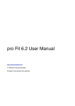

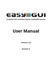
![PLAS A O ]-OR](http://vs1.manualzilla.com/store/data/005852706_1-5db0b7ed584537f0e62af161fb124638-150x150.png)