1
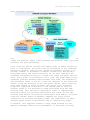
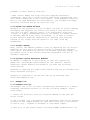
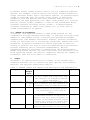
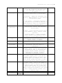
UNICOR user manual |1
UNICOR
USER MANUAL
Version: 2.0
Updated: 2012.03.22
Authors:
E. L. Landguth1, B. K. Hand1, J. M. Glassy1,2, S. A.
Cushman3
1 - University of Montana, Division of Biological Sciences, Missoula,
MT, 59812, USA.
2 - Lupine Logic Inc, Missoula, MT, 59802, USA.
3 - U.S. Forest Service, Rocky Mountain Research Station, 2500 S. Pine
Knoll Dr., Flagstaff, AZ 86001, USA
UNICOR user manual |2
Table of Contents
1
2
3
4
5
6
7
Introduction.................................................. 3
1.1 What can UNICOR do.................................... 3
1.2 How does UNICOR work.................................. 3
1.3 What‟s new in version 2.0............................. 6
Getting started............................................... 6
2.1 Dependencies.......................................... 6
2.1.1 Baseline requirements............................ 6
2.1.2 Python on non-windows platforms.................. 6
2.1.3 Python on windows................................ 6
2.1.4 Obtaining NumPy and SciPy........................ 7
2.2 Installation.......................................... 7
2.2.1 Installing Python, NumPy, and SciPy.............. 7
2.2.2 Unpack the UNICOR archive........................ 8
2.2.3 Install UNICOR................................... 8
2.2.4 Optional Python extension modules................ 8
2.3 Example run........................................... 8
2.3.1 Command line run................................. 8
Input......................................................... 9
3.1 Resistance grid....................................... 9
3.2 XY locations.......................................... 9
3.3 Types of paths........................................ 10
3.3.1 Dijkstra‟s shortest path......................... 10
3.3.2 Kernel density estimation on shortest path....... 10
3.3.3 Thresholding..................................... 10
3.3.4 Resistant kernel connectivity.................... 10
3.4 Number of processors.................................. 11
Output........................................................ 11
General issues................................................ 13
5.1 How to obtain UNICOR.................................. 13
5.2 Debugging and troubleshooting......................... 13
5.3 UNICOR limitations.................................... 13
5.4 How to cite UNICOR.................................... 13
5.5 Disclaimer............................................ 13
References.................................................... 14
Acknowledgements.............................................. 16
UNICOR user manual |3
1
Introduction
Habitat loss and its effects on populations of vulnerable species is
among the most urgent problems in conservation ecology. It is critical
that managers and scientists have effective tools to evaluate the
effects of landuse and climate change on the extent and connectivity
of populations. To address this need, we introduce UNIversal CORridor
network simulator (UNICOR), a species connectivity and corridor
identification tool. UNICOR applies Dijkstra‟s shortest path algorithm
to individual-based simulations. Outputs can be used to designate
movement corridors, identify isolated populations, quantify effects of
climate and management changes on population connectivity and
prioritize conservation plans to maintain population connectivity. The
key features include a driver-module framework, connectivity mapping
with thresholding and buffering, kernel resistance thresholding, and
calculation of graph theory metrics. Through parallel-processing,
computational efficiency is greatly improved, allowing analyses of
large extents (grid dimensions of thousands) and large populations
(individuals in the thousands).
1.1
What can UNICOR do
UNICOR is intended for use by land managers as well as the research
community and will be a valuable tool in applied conservation biology.
It provides new functionality to increase understanding of species
connectivity in current and future landscapes. This, in turn, provides
invaluable ability to quantitatively compare spatially explicit
conservation and restoration scenarios and prioritize actions to have
the largest cumulative effects on population connectivity. The results
can be used to designate sites as potential source or sink
populations, and identify corridors and barriers. Simulations could
address prioritizing areas of greatest concern, effects of climate
change on wildlife populations, or habitat fragmentation under future
climate or landuse change.
1.2
How does UNICOR work
UNICOR simulator uses a modified Dijkstra‟s algorithm (Dijkstra 1959)
to solve the single source shortest path problem from every specified
species location on a landscape to every other specified species
location. Figure 1 provides a step-by-step conceptual workflow. UNICOR
requires two input files as the first step: 1) a landscape resistance
surface and 2) point locations for each population or individual's
location (see section 3 for program input). Prior to running UNICOR,
users must create a resistance surface where each cell value (pixel)
represents the unit cost of crossing each location. Pixels are given
weights or „resistance values‟ reflecting the presumed influence of
each variable to movement or connectivity of the species in question
(e.g., Dunning et al. 1992; Cushman et al. 2006; Spear et al. 2010).
Resistance surfaces could be parameterized to reflect different costs
to movement associated with vegetation types, elevation, slope, or
UNICOR user manual |4
other landscape features.
Figure 1: UNICOR conceptual workflow diagram. Steps 1 and 2 define the
inputs and problem. Steps 3 and 4 execute the program. Step 5 provides
synthesis and post-processing.
Point locations define starting and ending nodes of paths connecting
pairs of individuals. The points must be referenced on the landscape
resistance surface, with any user specified placement pattern (e.g.,
uniform, random, or placement in habitat suitability) and density.
From graph theory and network analysis, we can then represent the
landscape resistance surface as a graph with nodes and edges (Diestel
2010). Every pixel is considered to be a node. The graph edges, which
represent possible movement paths between each node, are weighted by
the resistance value of the cell times the distance to the next pixel
center, times the distance to the next pixel center, which gives the
total edge length in terms of raster cell units (cost distance).
Dijkstra‟s algorithm is modified in the UNICOR code to find all
shortest paths to all destination nodes associated with the same
starting node. This provides a substantial boost in computational
efficiency where all pairwise combinations are found for the same
starting node before clearing the search space from memory. All paths
found are optimal paths of movement computed for every paired
combination of starting and ending nodes. The combination of these
shortest paths create a path density map or connectivity graph.
In essence, this approach becomes a large graph problem for the
applied landscape connectivity assessments. In analyses involving
UNICOR user manual |5
large numbers of individuals across a large and fine-grained
environment computational processing time becomes intractable.
However, parallel processing allows for efficient use of increasingly
ubiquitous, modern multi-core processors. Dijkstra's breadth-first
search algorithm is ideal for running in parallel for sets of source
and destination points because pairwise distances can be calculated
independently. We have implemented parallel processing in UNICOR using
the multiprocessing module from Python version 2.6. Parallel
processing in UNICOR is currently only implemented under the Linux
operating system.
To reflect species-specific differences in dispersal abilities, users
can specify connectivity thresholds. These connectivity thresholds are
expressed as the maximum path length for a species given its dispersal
ability. This enables UNICOR to realistically reflect the biological
dispersal abilities of a particular species. Users can specify the
maximum dispersal distance based either on cumulative cost distance or
Euclidean distance.
Dijkstra‟s base algorithm assumes the optimal is followed by all
individuals. However, this is unlikely to realistically represent the
behavior of organisms. Thus, it is beneficial to consider either
multiple low-cost paths, or to smooth output paths using a probability
density function such as a Gaussian bell curve (Cushman et al. 2008;
Pinto and Keitt 2008). UNICOR implements the latter and allows for
the application of a variety of smoothing functions referred to as
kernel density functions: Gaussian, Epanechnikov, uniform, triangle,
biweight, triweight, and cosine functions can be used for the kernel
density estimations (Li & Racine 2007). The outputs that are produced
by the program show the cumulative density of optimal paths buffered
by kernel density estimations (see Silverman 1986; Scott 1992)
following a distribution around frequency of common connections.
Through batch capability, users may specify alternative connectivity
thresholds to assess how scale dependency of dispersal ability will be
affected by landscape change and fragmentation under a range of
scenarios (e.g., Cushman et al. 2010a; Watts et al. 2010). Outputs
include paths among habitat patches that can be used to display
expected species movement routes and can provide managers with visual
guidance on identifying corridors that are likely critical for
maintaining network connectivity. Quantification of changes to habitat
fragmentation, and corridor connectivity is enabled through outputs of
graph theory metrics (e.g., density, number of nodes, radius, etc.)
(Hagberg et al. 2008) and connectivity outputs that can directly input
into popular landscape pattern analysis programs (e.g., FRAGSTATS
(McGarigal et al. 2002)).
The program is written in Python 2.6. UNICOR is built on a drivermodule, plug-in, docking architecture that allows for ease of future
modular development. The program‟s input parameters are organized as
name-value-pairs in a stanza oriented, text file format. The inputs
are parsed using the RipMgr package, a flexible symbol table manager
UNICOR user manual |6
for science models that includes special parsing capabilities (Glassy,
2010). UNICOR has been debugged as carefully as possible by testing
all combination of simulation options. The program is freeware and can
be downloaded at http://cel.dbs.umt.edu/software/UNICOR/.
1.3 What’s new in Version 2.0
Similar to connectivity thresholding, we have added a resistant kernel
approach for predicting habitat connectivity and corridor paths for
the given resistance surface as conducted by Compton et al. 2007.
Resistant kernel connectivity modeling has a number of advantages as a
robust approach to assessing population connectivity for multiple
wildlife species. First, unlike most corridor prediction efforts, it
is spatially synoptic and provides prediction and mapping of expected
movement rates for every pixel in the study area extent, rather than
only for a few selected “linkage zones” (Compton et al. 2007). Second,
scale dependency of dispersal ability can be directly included to
assess how species of different vagilities will be affected by
landscape change and fragmentation under a range of scenarios (e.g.,
Cushman et al. 2010a). Third, it is computationally efficient,
enabling simulation and mapping across vast geographical extents for a
large combination of species (e.g., Cushman et al. 2010b, Cushman et
al. 2011).
The resistant kernel approach to connectivity modeling uses the
framework of the modified Dijkstra‟s algorithm. Instead of calculating
one shortest path derived from source-to-source nodes, the resistant
kernel approach builds a least-cost dispersal around each source cell.
The resistant kernel approach implemented here uses the Dijkstra‟s
modified function to produce a map of movement cost from each source
up to a given specified threshold. Each source cost map is then
inverted and scaled with a given transformation function, such that
the maximum value for each individual kernel is one. Once the expected
density around each source location is calculated, the kernel maps
surrounding all sources are summed to give the total expected density
at each location on the landscape. The results of the resistant kernel
approach are surfaces of expected density of dispersing individuals at
any location in the landscape.
2
2.1
Getting started
Dependencies
2.1.1 Baseline Requirements
UNICOR requires the Python2.6.x interpreter (or greater but less than
Python3.0), NumPy package, and SciPy package. Several optional Python
module packages, if enabled, facilitate additional UNICOR
functionality. Remember that Python modules usually require particular
Python interpreters, so be sure the version ID for any external Python
module or package (e.g. NumPy or others) matches the version of your
Python interpreter (normally v2.6.x).
2.1.2 Python on Non-Windows Platforms
UNICOR user manual |7
Some common computer platforms come with Python installed. These
include MAC OS X and most Linux distributions. To determine which
Python a MAC or Linux workstation has installed, start a terminal
console and enter “python.” You'll see the version number on the top
line (enter Control-D to exit). Replacing an older Python interpreter
(pre v2.4) with a newer one (v.2.6.x) on a Linux or MAC OS X machine
can be tricky, so ask a System Administrator for help if you‟re not
sure which packages depend on the current Python installed.
2.1.3 Python on Windows
Windows (7, XP, 2000, Server) does not come with Python installed, so
follow the instructions below to obtain and install Python on a
computer running the Windows operating system. Get a windows
installation of the base Python installation (current v.2.6.x) at:
http://www.python.org/download/releases/ or see more details on other
python distributors below (e.g., ActiveState or Enthought).
2.1.4 Obtaining NumPy and SciPy
We recommend using the superpack Windows installer available from the
SourceForge website: http://sourceforge.net/project/. Note that more
complete information for NumPy is available at www.scipy.org, where
the SciPy module is also presented. Another source is
http://www.enthought.com/products/epd.php for a free academic and
educational usage in a single downloadable installer that has
everything and then some (Python, Numpy, Scipy, Matplotlib, and 70+
modules for python).
2.2
Installation
2.2.1 Install Python, NumPy, and SciPy
Make sure that Python and NumPy are installed, and available to you.
You can test this by typing "python" at a command window. If python is
available you'll get the python prompt ">>>". If it is not a
recognized command, it means either that python is installed but is
not in your command shell's paths, or that python is not installed. In
the first case ask an administrator to add it to your command paths
(or search for a tutorial on „How to set environmental path
variables”). If your shell locates and loads python, type, "import
numpy". Similarly, type, “import scipy”. If python does not complain
that there are no such modules, all is well.
The following instructions assume Python, NumPy, and SciPy are not yet
available on your computer; if they are, skip to section 2.2.2.
* First run the Python executable installer you've chosen (either from
www.python.org, ActiveState, or Enthought) accepting defaults for the
installation directory. On Windows this will typically place the
executables and libraries in c:/Python2.6/bin and the "site-packages"
package tree for user installed Python modules in
c:/Python2.6/lib/site-packages. If you are installing it on a network
on which you do not have administrative privileges, you may need to
ask a system administrator to install python and the NumPy and SciPy
UNICOR user manual |8
packages in their default locations.
* Next install NumPy and SciPy using the supplied executable
(superpack) installer or visiting http://www.scipy.org/Download. This
will install NumPy and SciPy in your Python ./site-packages directory.
Note if you used Enthought as a distribution, you already have NumPy
and SciPy installed and do not need this step.
2.2.2 Unpack the UNICOR Archive
Navigate to the directory on your PC where you wish to install UNICOR,
and unpack the supplied zip archive file using a free archive tool
like 7Zip (7z.exe), Pkunzip, Unzip, or an equivalent. Seven-Zip
(7Z.exe) is highly recommended since it can handle all common formats
on Windows, MAC OS X and Linux. On Windows, it is best to setup a
project specific modeling subdirectory to perform your modeling
outside of any folder that has spaces in its name (like "My
Documents").
2.2.3 Install UNICOR
Next, install the UNICOR software itself by unpacking the
supplied. At this point you should be able to execute the
test inputs. Alternatively and only for Windows operating
may double click on the unicorn_setup.exe executable file
automatic download.
zip archive
supplied
system, you
for an
2.2.4 Optional Python Extension Modules
As UNICOR is supplied in the archive, it does not require any
additional contributed Python modules to run. However, several
additional Python modules are needed if you want the following
functionality:
NetworkX is required for graph theory metrics and can be obtained from
http://networkx.lanl.gov/.
wxPython is required to run the GUI and can be obtained from
http://www.wxpython.org/.
2.3
Example run
2.3.1 Command line run
The example run is for 10 points representing individuals on a simple
landscape resistance surface. To run the following example, follow
these steps:
1. Locate the directory that you installed UNICOR to and open the
unicor folder.
2. The included .rip file specifies the parameters that can be changed
and used in the sample UNICOR run. Open small_test.rip in your editor
of choice (e.g., notepad or wordpad) to view these inputs.
3. This file is the stanza format following RipMgr documentation. All
UNICOR user manual |9
'#' signs are comments followed by variable names with a tab to the
parameter specified. The parameter can be changed for running UNICOR,
but downloaded parameters will run as is. See section 3 for more
details on each parameter along with its dependency.
4. Start the program at the command line: If you use Python from the
command line, then open a terminal window and change your shell
directory to the UNICOR home directory. For example in Windows you can
go to the Start Menu -> and open cmd.exe by searching for it or
locating it in Accessories. After ">" type cd
C:/LOCATIONOFYOURINSTALLATION.
5. Run the program: There are a number of ways to run this program.
For example, if you are using a command shell you can run the program
by typing “python UNICOR.py small_test.rip”.
6. Check for successful simulation run completion: The program will
provide a log file in your UNICOR home directory. Once completed,
output files will be created in UNICOR home directory. See section 4
for the description of outputs.
3
Input
See Table 1 for UNICOR inputs and outputs.
3.1 Resistance grid
Prior to running UNICOR, users must create a resistance surface where
each cell value (pixel) represents the unit cost of crossing each
location. Pixels are given weights or „resistance values‟ reflecting
the presumed influence of each variable to movement or connectivity of
the species in question. Resistance surfaces could be parameterized to
reflect different costs to movement associated with vegetation types,
elevation, slope, or other landscape. The filename for the resistance
surface must be in an ascii format with header file (any file
extension is acceptable, must be space delimited). The example
simulation run resistance grid is small_test.rsg and will provide
format example.
3.2 XY locations
Point locations define starting and ending nodes of paths connecting
pairs of individuals. The points must be referenced on the landscape
resistance surface, with any user specified placement pattern (e.g.,
uniform, random, or placement in habitat suitability) and density. The
filename for the individuals with (x,y) locations can have any file
extension, but must be comma delimited. In addition, points must fall
in a unique pixel of the resistance grid, i.e., the point spacing
should be greater than the resolution of your resistance grid times
the square root of two. If you have overlapping points, the program
will display the following error message, “There are overlapping
points around x = ' ' and y = ' ', please check for points that are
too close together. This point will not be included in the run.” The
example simulation run XY locations file is small_test_10pts.xy and
will provide format example.
U N I C O R u s e r m a n u a l | 10
3.3
Types of paths
3.3.1 Dijkstra’s shortest path
UNICOR can calculate all pairwise shortest path or least-cost paths
for the XY locations specified when the „Edge_Type‟ is set to
„normal‟. Warning, this is a large graph program and if you have a
large number of points and/or large number of pixels in your
resistance grid, then we recommend running this option in parallel.
See section 3.4 for more details. You can also use UNICOR to calculate
the Euclidean distance between all individual XY locations by
specifying „Use ED Threshold‟ to TRUE. This is a fast calculation and
no need to run in parallel.
3.3.2 Kernel density estimation on shortest paths
Dijkstra‟s base algorithm assumes the optimal path is followed by all
individuals. However, this is unlikely to realistically represent the
behavior of organisms. Thus, it is beneficial to consider either
multiple low-cost paths, or to smooth output paths using a probability
density function such as a Gaussian bell. UNICOR implements the latter
and allows for the application of a variety of smoothing functions
referred to as kernel density functions: Gaussian, Epanechnikov,
uniform, triangle, biweight, triweight, and cosine functions can be
used for the kernel density. The outputs that are produced by the
program show the cumulative density of optimal paths buffered by
kernel density estimations following a distribution around frequency
of common connections.
3.3.3 Thresholding
To reflect species-specific differences in dispersal abilities, users
can specify connectivity thresholds. These connectivity thresholds are
expressed as the maximum path length for a species given its dispersal
ability in cost units. This enables UNICOR to realistically reflect
the biological dispersal abilities of a particular species. Users can
specify the maximum dispersal distance based either on cumulative cost
distance or Euclidean distance. To set the threshold for cost units,
specify „Edge_Type‟ to „threshold‟ and use a specified „Edge Distance‟
that is in cost units or your resistance grid. To set the threshold
for Euclidean distance, make sure that „Use ED Threshold‟ is TRUE and
specify a Euclidean distance in the field „ED Distance‟.
3.3.4 Resistant kernel connectivity
Similar to kernel density estimation, resistant kernel connectivity
modeling does not assume an optimal path. Instead kernel maps are
produced for each source point and added together to give the expected
density of dispersing organisms at any location on the landscape
surface. See Compton et al. 2007 for more details. To use this
function, set „Edge_Type‟ to „all_paths‟. This function will use the
field „Edge Distance‟ to calculate a resistant kernel to a threshold
(note that „Edge Distance‟ is in cost units). In addition, a
„Transform function‟ can be specified for how each source‟s resistant
kernel is scaled. A „Constant Kernel Volume‟ can be enforced, as well.
U N I C O R u s e r m a n u a l | 11
A constant kernel volume could be used if you are comparing different
species. For example, a mobile species can travel farther producing a
larger resistant kernel than a less-mobile species. If constant kernel
volume is enforced, then the volume of the kernel is essentially
population size and species that have different mobility can be
modeled at the same population size. When „const_kernel_vol‟ is False,
then the „kernel_volume‟ parameter is used on the transformed kernel
resistant distance following „kernal_volume‟ * 3/(math.pi*kernel
resistant distances^2). When „const_kernel_vol‟ is True, then no
volume transformation is applied.
3.4 Number of processors
In essence, this approach becomes a large graph problem for the
conservation biology problems faced today. In analyses involving large
numbers of individuals across a large and fine-grained environment
computational time becomes intractable. However, parallel processing
allows for efficient use of increasingly ubiquitous, modern multi-core
processors. Dijkstra's breadth-first search algorithm is ideal for
running in parallel for sets of source and destination points because
pairwise distances can be calculated independently. We have
implemented parallel processing in UNICOR using the multiprocessing
module from Python version 2.6, and is currently only available in the
Linux operating system. For parallel computing, specify the „Number of
Processors‟ that are to be used in a simulation.
4
Output
See Table 1 to specify which files to output. Files include ascii
formatted surfaces for all connectivity path options, cost distance
matrices, and optional graph theory metrics.
Table 1: UNICOR inputs and outputs with description and dependencies.
Input Name
Default/
Description
Example
Input
Grid Filename small_te The filename for the resistance surface
st.rsg
in ascii format with header file (any
file extension is acceptable, must be
space delimited).
XY Filename
small_te The filename for the individuals with
st_10pts (x,y) locations (any file extension is
.xy
acceptable, must be comma delimited).
Use ED Threshold False
Option for calculating Euclidean
distance between all pairwise points.
Use thresholding in next field as
option.
ED Distance
50000
If Use ED threshold is True, then this
is Euclidean distance in map units to
apply to the (x,y) point locations. If
you want all Euclidean distance values,
specify this value to be greater than
the maximum distance on your map.
Edge Distance
100000
The resistance distance threshold in
terms of edge distance or cost units to
Dependency
U N I C O R u s e r m a n u a l | 12
Edge_Type
Normal
apply to the path lengths between each
pair of XY locations. Use this value
with Edge_Type „threshold‟ and
„all_paths‟.
'normal' – All pairwise shortest costdistance paths with no thresholding.
'threshold' – Apply the threshold value
given by „Edge Distance‟ to all shortest
cost-distance paths.
Transform
function
Linear
'all_paths' – Calculate resistant
kernels for all XY locations and use the
„Edge Distance‟ value as a threshold for
each source resistant kernel.
Specify the scaling away from the
sources point used in the resistant
kernel model.
'linear' – Scale resistant kernel values
to be between 0 and 1, using a linear
function.
„inverse_square‟ – Scale resistant
kernel values to be between 0 and 1,
using an inverse-square function.
Keep resistant kernel volume constant
Constant kernel True
for each XY location and equal to 1.
vol
Option „True‟ or „False‟
10000
Set the resistant kernel volume to this
Kernel Volume
value when Const_kernal_vol is „False.
Number of
8
For parallel computing, the number of
Processors
processors that are used in a
simulation.
KDE Function
Gaussian
For kernel density estimation of
„normal‟ paths, this is the probability
distribution used to calculate the
kernel density buffer [Gaussian,
Epanechnikov, Uniform, Triangle,
Biweight, Triweight, Cosine].
KDE GridSize
2
For kernel density estimation of
„normal‟ paths, this is the kernel
buffer window used to calculate the
buffered maps. For example if 2, then 2
pixel values around each path is used to
create the kernel density buffer.
Number of Levels
3
For kernel density estimation of
„normal‟ paths, this is the number of
categories used to display the kernel
density buffer map. If 3, then this
option will take the kernel density
buffer created and categorize the values
into 3 equal-interval classes (low,
medium, high).
Output
Default/
Example
Description
Linux
SciPy
SciPy
SciPy
Dependency
U N I C O R u s e r m a n u a l | 13
Save Path Output
Input
TRUE
Save Individual
Paths Output
FALSE
Save Cost
Distance Matrix
Output
Save KDE Output
TRUE
5
FALSE
Save Levels
Output
FALSE
Save Graph
Metrics Output
FALSE
The surface of paths in ascii format
with header file (space delimited –
.addpaths).
The list of individual path values and
length from every point to every other
point (comma delimited - .paths). This
can be a very large file depending on
the size of your problem.
The resistance distance matrix of all
the source-destination connection
lengths (comma delimited - .cdmatrix).
The surface of kernel density buffered
paths in ascii format with header file
(space delimited – .kdepaths).
The categorical surface created from the
KDE output in ascii format with header
file (space delimited - .levels)
Path graph theory metrics (comma
delimited - .graphmetrics)
NetworkX
General issues
5.1 How to obtain UNICOR
The program is freeware and can be downloaded at
http://cel.dbs.umt.edu/software/UNICOR/ with information for users,
including manual instructions, FAQ, publications, ongoing research,
and developer involvement.
5.2 Debugging and troubleshooting
For help with installation problems please check first for postings at
our web site. Otherwise, please report problems including any bugs, to
me at [email protected].
5.3 UNICOR limitations
The following is a list of the current (as we know of) limitations
with UNICOR:
1. The resistance surface is in ASCII format: header file with 6 lines
of information and space delimited.
2. The point locations have a header row and file is comma delimited.
3. Point locations must fall inside the resistance grid extent. The
code will run when points lie outside of grid, but no paths will be
calculated.
4. The point locations must lie in a unique pixel or cell in the
resistance surface.
5. Graph metrics will only run on small problems and not implemented in
parallel.
5.4 How to cite UNICOR
This program was developed by Erin Landguth, Brian Hand, and Joe
Glassy. GUI development was done by Mike Jacobi. Ross Carlson assisted
with graphics, data set, and website creation. The reference to cite
U N I C O R u s e r m a n u a l | 14
is:
Landguth EL, Hand BK, Glassy JM, Cushman SA, Sawaya, M (2011) UNICOR:
A species connectivity and corridor network simulator. Ecography, 34,
1-6.
5.5 Disclaimer
The software is in the public domain, and the recipient may not assert
any proprietary rights thereto nor represent it to anyone as other
than a University of Montana-produced program (version x.x). UNICOR is
provided "as is" without warranty of any kind, including, but not
limited to, the implied warranties of merchantability and fitness for
a particular purpose. The user assumes all responsibility for the
accuracy and suitability of this program for a specific application.
In no event will the authors or the University be liable for any
damages, including lost profits, lost savings, or other incidental or
consequential damages arising from the use of or the inability to use
this program.
We strongly urge you to read the entire documentation before ever
running UNICOR. We wish to remind users that we are not in the
commercial software marketing business. We are scientists who
recognized the need for a tool like UNICOR to assist us in our
research on landscape ecology issues. Therefore, we do not wish to
spend a great deal of time consulting on trivial matters concerning
the use of UNICOR. However, we do recognize an obligation to provide
some level of information support. Of course, we welcome and encourage
your criticisms and suggestions about the program at all times. We
will welcome questions about how to run UNICOR or interpret the output
only after you have read the entire documentation. This is only fair
and will eliminate many trivial questions. Finally, we are always
interested in learning about how others have applied UNICOR in
ecological investigation and management application. Therefore, we
encourage you to contact us and describe your application after using
UNICOR.
We hope that UNICOR is of great assistance in your work and we look
forward to hearing about your applications.
6
References
Bunn,A.G., Urban,D.L. and Keitt T.H. (2000) Landscape connectivity: A
conservation application of graph theory. Journal of Environmental
Management, 59, 265-278.
Compton,B., et al. (2007) A resistant kernel model of connectivity for vernal
pool breeding amphibians. Conservation Biology, 21, 788–799.
Cushman,S.A., et al. (2006) Gene flow in complex landscapes: testing multiple
hypotheses with casual modeling. The American Naturalist, 168, 486-499.
Cushman,SA, McKelvey,K.S. and Schwartz,M.K. (2009) Use of empirically derived
source-destination models to map regional conservation corridors.
Conservation Biology, 23, 368-376.
U N I C O R u s e r m a n u a l | 15
Cushman,S.A., Chase,M.J. and Griffin,C. (2010a) Mapping landscape resistance
to identify corridors and barriers for elephant movement in southern Africa.
In Cushman,S.A. and Huettman,F. (eds). Spatial complexity, informatics and
wildlife conservation, Springer, Tokyo, pp. 349-368.
Cushman,S.A., Compton,B.W. and McGarigal,K. (2010b) Habitat fragmentation
effects depend on complex interactions between population size and dispersal
ability: Modeling influences of roads, agriculture and residential
development across a range of life-history characteristics. In Cushman,S.A.
and Huettman,F. (eds). Spatial complexity, informatics and wildlife
conservation, Springer, Tokyo, pp. 369-387.
Dale,V.H., et al. (2001) Climate change and forest disturbances. BioScience,
51, 723-734.
Diestel,R. (2010) Graph Theory, Springer-Verlag, Heidelberg, Fourth Edition.
Dijkstra,E.W. (1959) A note on two problems in connexion with graphs.
Numerische Mathematik, 1, 269–271.
Dunning,J.B., Danielson,B.J. and Pulliam,H.R. (1992) Ecological processes
that affect populations in complex landscapes. OIKOS, 65, 169 -175.
Fall,A., et al. (2007) Spatial graphs: principles and applications for
habitat connectivity. Ecosystems, 10, 448-461.
FAO (2006) Global Forest Resources Assessment 2005, Main report. Progress
towards sustainable forest management, FAO Forestry Paper 147, Rome, p 320.
Hagberg,AA., et al. (2008) Exploring network structure, dynamics, and
function using NetworkX, In Varoquaux,G., et al. (eds) Proceedings of the 7th
Python in Science Conference (SciPy2008), Pasadena, CA USA, pp. 11-15.
McGarigal,K., et al. (2002) FRAGSTATS: Spatial Pattern Analysis
Program for Categorical Maps. Computer software program produced by the
authors at the University of Massachusetts, Amherst. Available at the
following web site:
http://www.umass.edu/landeco/research/fragstats/fragstats.html
McRae,B.H. and Beier,P. (2007) Circuit theory predicts gene flow in plant and
animal populations. Proceedings of the National Academy of Science USA, 104,
19885-19890.
McRae,B.H., et al. (2008) A multi-model framework for simulating wildlife
population response to land-use and climate change. Ecological Modelling,
219, 77-91.
Li,Q. and Racine,J.S. (2007) Nonparametric Econometrics: Theory and Practice.
Princeton University Press.
Opdam,P. and Wascher,D. (2003) Climate change meets habitat fragmentation:
linking landscape and biogeographical scale levels in research and
conservation. Biological Conservation, 117, 285-297.
Pinto,N. and Keitt,T.H. (2009) Beyond the least cost path: evaluating
U N I C O R u s e r m a n u a l | 16
corridor robustness using a graph-theoretic approach. Landscape Ecology, 24,
253-266.
Riitters,K. et al. (2000) Global scale patterns of forest fragmentation.
Conservation Ecology, 4, [online] URL:
http://www.consecol.org/vol4/iss2/art3/
Sawyer,H., et al. (2009) Identifying and prioritizing ungulate migration
routes for landscape-level conservation. Ecological Applictions, 19, 20162025.
Scott,D.W. (1992) Chapter 6. In: Multivariate Density Estimation; Theory,
Practice, and Visualization. John Wiley and Sons, New York.
Schwartz,M.K., et al. (2009) Wolverine gene flow across a narrow climatic
niche. Ecology, 90, 3222-3232.
Silverman,B.W. (1986) Chapter 3. In: Density Estimation for Statistics and
Data Analysis. Chapman and Hall, New York.
Spear,S.F., et al. (2010) Use of resistance surfaces for landscape genetic
studies: Considerations for parameterization and analysis. Molecular Ecology,
in press.
Urban,D. and Keitt,T. (2001) Landscape connectivity: A graph-theoretic
perspective. Ecology, 82, 1205-1218.
Watts,K., et al. (2010) Targeting and evaluating biodiversity conservation
action within fragmented landscapes: an approach based on generic focal
species and least-cost networks. Landscape Ecology, 25, 1305-1318.
7
Acknowledgements
This research was supported in part by funds provided by the Rocky
Mountain Research Station, Forest Service, U.S. Department of
Agriculture and by the National Science Foundation grant #DGE-0504628.