Download 3D Grid Generation

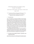
3D Grid Generation
Sven H.M. Buijssen
FeatFlow Springschool 2002
Abstract
In this paper it will be explained how to create the geometry and the mesh needed for a 3D
simulation with FeatFlow. Up to now, there are two separate ways: a semi-automatic and a
manual fashion. On a midterm range FeatFlow/DeViSoR interfaces to professional CAD and grid
generation software will probably become available such that there will be a third and, simultaneously,
more convenient way of 3D preprocessing. But currently you only have the choice between two
possibilities. In most cases the problem’s geometry determines which path to follow.
1
From 2D to 3D via extrusion
1.1
General
Some 3D geometries can be reduced to a 2D problem. This is because they are symmetric in (at least)
one space direction. Consider, for instance, the problem of flow within a unit cube which is a very
common test problem to start with. Or a problem that is little bit more challenging: flow around a
cylinder in a rectangular box. If you squeeze the box together, you end up with a 2D problem: flow
around a circle. So, if you have a geometry description and a mesh for this 2D problem (and everybody
following this course already has one: the 2D DFG Benchmark created with DeViSoRGrid), it is quite
natural to put two or more copies of the 2D mesh in succession. Creating an edge between those two
nodes of neighbouring mesh layers that have the same (x, y)-coordinates will result in a 3D mesh (see
Figure 1.1). This extrusion process can be performed automatically. FeatFlow ships with a small
Figure 1: Creating a 3D mesh via extrusion
utility program called tr2to3. If you already have a prm file (containing the 2D geometry definition)
and a tri file (containing the 2D mesh), tr2to3 generates a tri file containing the 3D geometry as
well as the mesh1 . Having created this mesh you can test it with trigen3d or even start a 3D flow
simulation with cc3d/cp3d/pp3d/parallel pp3d++.
1.2
Configuring tr2to3
Using tr2to3 is quite simple because there are only a few parameters you have to remember respectively adjust. In the case of a 3D problem that can be reduced to a 2D problem, you are almost
finished once you have designed the 2D geometry and mesh (using DeViSoRGrid or even manually).
Let’s have a look at a sample tr2to3 configuration file (see Table 1.2).
1 There
is no equivalent of the 2D parametrisation in 3D
1
1
FROM 2D TO 3D VIA EXTRUSION
==============================================================
File for input data for tr2to3
==============================================================
2
M
1
MT
1
ICHECK
1
IMESH (0=FEAT-parametrization,1=tri+prm file)
’dfg2d.prm’
CPARM (name of parametrisation file)
3
IGMV
(level for GMV-output)
0
IAVS
(level for AVS-output)
’dfg2d.tri’
CFILEI (name of input file)
’dfg3d.tri’
CFILEO (name of output file)
8
NPZ
(number of z-levels)
0.0D0
PZMIN
0.41D0
PZMAX
0.05125
0.1025
0.15375
0.205
0.25625
0.3075
0.35875
Table 1: Listing of a sample tr2to3.dat
Let us assume that you followed the steps explained in the talk on 2D grid generation or within
the DeViSoRGrid 2 User’s Manual respectively [2]. Moreover, it is assumed that the example you
created (2D DFG benchmark) is stored using the file names ’dfg2d.prm’ and ’dfg2d.tri’.
Our aim is to create a rectangular box with a depth of 0.41 metres consisting of 9 layers of 2D
mesh slices. This will give us a 3D mesh with 8 hexahedrons in z-direction (i.e. 8 ”z-levels”). There
is no need to design the mesh equidistant in z-direction but in our example it is.
Let us examine the sample configuration file line by line and explain the respective meaning:
M, MT These two parameters control the verbosity of the program during the conversion process.
The higher the value, the more messages are printed to disk and on your terminal. Default
values of 2 and 1 respectively are appropriate for every day use.
ICHECK obsolete parameter
IMESH This parameter is a toggle switch which controls whether you have a tri+prm file pair (1)
or only a tri file (0). In the latter case the parametrisation is coded in F77 and compiled into
tr2to3 itself. If you used DeViSoRGrid to create the 2D geometry and mesh, set this parameter
to 1.
CPARM This string contains path and file name of the parametrisation file or is left empty if
IMESH is set to 0.
IGMV If set to a value greater than zero, a grid file is created that can be visualised using GMV.
If set to a value of 2 or higher, the 3D grid is even refined once or more such that the grid on
refinement level 2 or higher is exported.
IAVS The same for the visualisation program AVS.
CFILEI This string contains path and file name of the triangulation file.
CFILEO If your 2D input data is feasible and the configuration data is set up properly, a file with
the 3D grid information is created using this string.
NPZ The number of elements that will be created in z-direction, i.e. the number of copies of 2D
grids put in succession diminished by one.
PZMIN z-coordinate of first ”2D mesh layer”
PZMAX z-coordinate of last ”2D mesh layer”
trailing floats z-coordinate of every ”2D mesh layer” inbetween
2
2
CREATING A 3D GRID MANUALLY
1.3
Creating the mesh
One you have carefully configured tr2to3, the remaining step is invoking the program and checking
whether the resulting grid looks like you anticipated. For this, you need a visualisation program like
GMV or AVS [1].
2
Creating a 3D grid manually
In the preceding section you were told how to take advantage of some symmetry properties of a
3D geometry. Unfortunately, it is not always possible to reduce the generation of a 3D grid to the
generation of a 2D grid followed by a simple extrusion procedure. So, if you want to create grids
for more general problems, you need to learn about the internal structure of a 3D grid file. If you
know how to read these columns of integers and floating point numbers you can modify and enhance
existing grids quite easily. You can even create grids from scratch using nothing more than an ASCII
editor (and probably a pencil, some pieces of paper and quite an amount of spatial imagination).
2.1
Syntax of a 3D grid file
The first two lines of a 3D grid file are considered as comments. Thus, they are ignored by all
FeatFlow programs. They have no other purpose but being a distinguishing badge for you in order
to be able to organise the medley of grids you collect in the course of time.
The third line contains summary information on the current grid: six integer values separated by
white spaces specifying the total number of elements, vertices, boundary components, vertices per
element, edges per element and faces per element.
The key word DCORVG indicates the beginning of the section with the coordinates of every node.
The first node implicitly gets the (internal) number 1. In total, exactly that number of nodes is
expected as was specified in line 3 (NVT). A departure will not be tolerated and will probably cause
a crash of trigen3d or your flow simulation program.
The key word KVERT indicates the beginning of the element definition section. In 3D flow simulation, we encourage you to use hexahedrons instead of pyramids. Especially if you have to create your
grids manually, you should act on this advice. So, how do you code a single hexahedron?
A hexahedron is determined by a sequence of eight numbers indicating the eight vertices. To get
a unique definition you have to reckon with a certain order – like in 2D [2]. The first four numbers
must indicate nodes that are vertices of one single face of the hexahedron. In addition, they must
be ordered counterclockwisely. The remaining four nodes must belong to the opposite face of the
hexahedron and are ordered in counterclockwise sense as well. The final condition is that there has
to be an edge between the first and the fifth vertex in the sequence.
Having defined the coordinates of every node and having connected them to build elements you
are nearly done. Last thing to do is to specify for each node which boundary component it belongs
to. The section for this so-called nodal property starts with the key word KNPR. Inner nodes get a 0,
boundary nodes the number of the boundary component they belong to.
Again, there is little tolerance in case of mistakes: if you add some nodes manually to a grid file,
adjust the total number of vertices in line 3, but you forget to specify the nodal property of these new
nodes, the 3D FeatFlow programs will give a (possibly enlightening) error message and terminate.
As an example Table 2.1 shows a grid that consists of 4 cubes, arranged two by two. Using
trigen3d you can visualise the grid with GMV or AVS.
This is everything you need to know about 3D grid generation. Good luck and have some fun!
3
3
SOME REMARKS
4
Grobgitter TRIAC1
4 cubes
4 18 1 8 12 6
NEL NVT NBCT NVE NEE NAE
DCORVG
0.0 0.0 0.0
0.5 0.0 0.0
Z
0.5 0.5 0.0
0.0 0.5 0.0
0.0 0.0 0.5
13
16
0.5 0.0 0.5
0.5 0.5 0.5
14
0.0 0.5 0.5
15
1.0 0.0 0.0
5
8
17
1.0 0.5 0.0
18
1.0 0.0 0.5
6
1.0 0.5 0.5
7
0.0 0.0 1.0
4
1
0.5 0.0 1.0
11
12
0.5 0.5 1.0
0.0 0.5 1.0
2
3
1.0 0.0 1.0
1.0 0.5 1.0
9
10
KVERT
1 2 3 4 5 6 7 8
X
2 9 10 3 6 11 12 7
5 6 7 8 13 14 15 16
6 11 12 7 14 17 18 15
KNPR
1 1 1 1 1 1 1 1 1 1 1 1 1 1 1 1 1 1
Y
Table 2: Sample 3D tri file and the corresponding grid
3
Some remarks
Within this paper two methods to create a 3D grid for FeatFlow usage were presented. As long
as we do not have interfaces to professional CAD and grid generation software you will have to cope
with either method.
Of course, you can combine these methods, too. As explained, 3D grids that are created using
tr2to3 will describe a geometry where objects are clamped between the lateral walls (e.g. a cylinder
fixed at the walls). If you want a freely floating object in your box (e.g. a short cylinder, a car etc.),
you will have to add manually additional element slices at the lateral walls.2
Strictly speaking, there is also a third possibility to describe a geometry with FeatFlow that
was not mentioned yet here. But it was already mentioned in the talk on ”ppxd and movbc solvers”
by Dr. D. Wan [3]. Especially if you have moving or free boundaries this third possibility is quite
convenient. One can use a technique called ”fictitious boundary conditions”:
In a few words, the information on inner boundaries is not at all coded into a tri file, the tri file
describes only the outer boundary. Obstacles and other inner objects that influence the flow pattern
are directly coded into FeatFlow (bndry.f) – analytically. Each time boundary values are to be set,
velocity and pressure values for every inner nodes whose coordinates lie outside of an inner boundary
are reset to zero. Inner nodes which reside directly on an inner boundary have their Dirichlet or
Neumann boundary values reassigned. This technique was for instance applied to simulate a rotating
propeller flow in a channel (http://www.featflow.de/album/contents5.html).
And last but not least: If you have a rotationally symmetrical geometry in 3D, one can use polar
coordinates to reduce the problem to 2D. As a matter of fact, we already did this once and wrote
2 At
least for the near future. But we plan to develop a tool that does this automatically as well.
REFERENCES
a code to solve the Stokes problem for rotationally symmetrical domains. This piece of software,
however, is definitely not ready to be published. Maybe we find someone in the near future to
re-implement this and who extends the code to incompressible Navier-Stokes problems.
References
[1] J. Acker, Postprocessing in FeatFlow
[2] D. Göddeke, DeViSoRGrid 2 User’s Manual.
[3] D. Wan, The ppxd and movbc solvers.
5