1
Visual Environment for the Taylor integration in 3D Stereo
Alexander Gofen
The Smith-Kettlewell Eye Research Institute, 2318 Fillmore St.,
San Francisco, CA 94115, USA
A cross-platform application called the Taylor Center implements advanced user interface and 2D or 3D stereo
dynamic visualization of the solution. It integrates ODE's using the Modern Taylor method, having unlimited
order of approximation, finite step, and high accuracy, allowing to explore or export the solution in different
formats. Designed in Delphi-6, the package implements a powerful Graphical User Interface, and is portable to
windowed versions of Linux too.
Introduction
What we expect from an application with
advanced interactive visualization is:
(a) User interface whose style, controls, and
handlers fit best for the specific model and
operational tasks;
(b) Realistic visualization of the modeled
process employing all appropriate faculties of the
human perception, achievable with advanced
hardware and multimedia.
With that in mind we consider a general
purpose program called the Taylor Center, which
performs integration of initial value problems for
systems of Ordinary Differential Equations
(ODE's) [7,8]. Unlike earlier packages [1,2], this
sophisticated Taylor Solver is designed for PCs as
an interactive application with extensive Graphical
User Interface. Moreover, it was developed in a
programming environment which exemplified the
Visual programming and made its good name: the
Borland's Delphi (a dialect of Pascal having such
advance features as dynamic arrays, objects, and
sophisticated graphics). Actually the software may
be considered as a cross platform Windows/Linux
project because Borland offers also a Linux
implementation of Delphi (called Kilex).
Although not any mathematical object may be
readily visualized, the solutions of ODE's are, as
their geometrical interpretation is trajectories in
Euclidian space En (planar curves for n=2). In a
computerized world we can expect not just still
images of trajectories, but also real time animation
of the motion along them, and we can even expect
visualization for n=3 too.
This All-In-One application is called the
Taylor Center (according to the metaphor of a
"Music Center") because it offers an interactive
environment, where researchers can input (import)
ODE's in symbolic format, vary the parameters,
explore the Taylor expansions and their
convergence radius, integrate the equations with
high accuracy (up to all available float point digits),
store or export the results, graph the solutions and
"play" them dynamically as bullet trajectories in
real time animation. The feature making this
application unique is that it can display non-planar
3D trajectories as anaglyphic stereo viewed
through Red/Blue glasses [6,7]. In particular, it
implements a 3D cursor (controlled by a
conventional mouse). This cursor with "tactile"
audio feedback allows users to "touch" points of
non-planar curves hanging in thin air, while
viewing the current 3D coordinates. Here the
multimedia is employed in its full capacity
(especially because of the stereo viewing – not yet
ubiquitous in the computer world).
Particularities of the 3D visualization
The perspective drawing of 3D world
(isometry) is known for a couple of centuries.
Human imagination easily interprets perspectively
correct planar images of common objects,
especially those with strong perspective cues, but
that is not always the case, and then human
capability of stereo perception and tools for stereo
vision come to play.
Stereo vision is a powerful ability of our brain
to recreate an image of 3D scene1 "fusing" the two
planar images received by the eyes [3, 6]. Mental
image of 3D space belongs completely to the realm
of imaginary sensations, because there is no place
in our body where any kind of 3D replica of reality
is materialized. The only physical replica we do
1
Mathematically speaking, recreation of the 3D scene
from a pair of 2D images is not a well defined
problem, and it may have multiple solutions.
have is the two planar images on the retina of our
eyes.
The real excitement of the 3D vision happens
when we look at objects expected to be planar (a
screen, a hologram), but the brain suddenly
discovers a 3D scene in it, popping out from the
planar surface or shifting back into the depth.
This is the 3D Stereo Vision, or the real 3D –
not to be confused with the misnomer "3D
Graphics" used for video cards and video libraries.
This misleading term emerged when the game and
video technology switched from simplistic
projections (known as front, side and top views in
drawing) to a more advanced oblique projection of
3D scenes. Photos, isometric drawings, artistic
paintings (if their perspective is correct) all are
examples of such projection. When we look at
them, we perceive them exactly as planar 2D
projections of 3D reality2.
We have all become good at "reading" these
projections and understanding the 3D reality they
represent. Such projections were the closest we
could come to 3D imagery until invention of the
stereoscope in 19th century in Great Britain.
The two eyepieces of a stereoscope deliver
the two planar images of a stereo pair directly to
the respective eyes. Then a miracle occurs: viewers
perceive the 3-dimesionality of the scene as real –
so real that they wish to touch the objects hanging
in air. This never happens when we look at 2D
projection of the 3D world.
After the stereoscope, many other techniques
were developed for displaying 3D stereo images
[4]. Except for the holograph, they all use the same
basic principle as the stereoscope: to deliver each
of the two images of a stereo-pair to the proper
(and only to the proper) eye. On the contrary, the
holographic equipment completely reproduces the
3D light front, i.e. the 3D vector field of the same
electromagnetic waves that would be reflected by
the 3D scene if it were really there. Thus a
hologram creates a sculptural "ghost" in the real
world as a physical phenomenon – a 3D scene we
view by a pair of eyes, while a stereo pair creates
this scene in our mind – an ultimate addressee
anyway. Another fundamental difference is in the
2
Binocular viewing of a perspectively correct planar
image creates perception of a planar drawing only:
isometric or not, yet in a plane. That is because this
plane is the solution corresponding to the 3D reality
encoded in this stereo pair. Surprisingly enough, if the
same isometry is viewed by one eye at the
perspectively correct distance, with a little effort the
brain does generate the stereo perceptions of this very
scene reconstructing it out of the perspective cues – a
phenomenon called monocular stereopsis.
quantity of information: a stereo pair is just two
planar images, while a hologram encodes (almost)
infinity of them.
Does the stereo vision give some advantages
vs. a planar perspective projection of a 3D scene?
The isometrics (or photo-imaging) suffice in many,
but not in all situations. In displaying such objects
as scenes with rectangular shapes, bodies with
edges, skeletal structures, scenes with good
perspective cues or with reflection hints, isometry
is good enough. For them, the stereo viewing only
adds certain excitement in perception.
Yet the isometrics works poorly for smooth
surfaces without edges (smooth 2D manifolds). For
example, to perceive a picture of a sphere or a
torus, we additionally draw grids on their surfaces,
or special shadows and reflections. The 2D
projections become especially inefficient while
visualizing non-planar curves (1D manifolds) – and
that is what solutions of ODEs are. For example,
trajectories of space probes launched to planets of
Solar system are usually non-planar. To draw them
in conventional isometry we need to add several
auxiliary planes and referencing coordinate lines.
The real stereo viewing eliminates necessity in all
auxiliary hints (see the 3D demo samples). Thus,
displaying non-planar solutions of ODEs in 3D
stereo dramatically improves the perception3.
This particular software employs the cheapest
technical realization of stereo vision, known as
anaglyph stereo, which requires nothing more than
a conventional PC monitor plus cardboard glasses –
the cheapest gear possible [6]. The two images of
an anaglyphic stereo pair must be monochromatic –
each in a different color (one of the basic
Red/Green/Blue set). The Red/Blue pair is better
because their spectrums are farther away from each
other and better separable. When you look through
the Red/Blue glasses at the Red/Blue images of a
stereo pair that overlap on a screen, each eye
receives only the proper image of the stereo pair.
How does the brain fuse stereo pairs
presented in different colors? After all it evolved
and is trained to match corresponding elements of
stereo pairs, and the corresponding elements must
be of the same color indeed.
Fortunately, the brain follows not a "rigid",
but rather a "flexible" algorithm. Certain neurons
fire if they find out recognizable elements in the
image disregarding their colors, while the others
There are many other cases when stereo viewing
becomes essential, being implemented in various
equipment from micro- to telescopes [4]. For example it
is used to visually detect counterfeit bills, or changes in
aerial photos of landscapes.
3
fire if these elements happen to comprise a
"meaningful" stereo pair. The signals of those
"stereo-specialized" neurons dominate. As a result
we easily fuse the 3D scene in spite of the fact, that
each eye sees it in a different color. This works
well both on a PC monitor for a single viewer, and
with a screen projector for a large audience.
The modern technology nowadays offers a
variety of other technical solutions with completely
uncompromised stereo viewing.
Particularities of the integration method:
more than tabulated functions
The method of integration implemented in
this software is the modern Taylor method – to be
distinguished from its classical counterpart in that
the process of n-order differentiation was
optimized and made feasible due to the concepts of
Automatic Differentiation (AD) and (generalized)
elementary functions [5].
Among other methods of integration, the
Taylor method is situated somewhere between
purely numerical methods and symbolic
integration. However, unlike purely numeric
methods, it delivers not only tabulated values of
unknown functions in point of interests, but also
their derivatives up to any specified order (default
30) and convergence radius at every point. And
unlike symbolic integration, the Taylor method
applies not only to very limited list of ODEs
solvable in quadratures, but to any ODEs in regular
points of the phase space.
From the programmatic point of view, any
Taylor solver differs from conventional integrators
in that the input – an Initial Value Problem for
ODEs – should be provided not simply as a
subroutine computing the right hand parts, but
rather as arithmetic expressions themselves of
those right hand parts in order to enable automatic
differentiation (understood as optimized classical
formulas for n-th order derivatives applied to
sequences of basic expressions).
Correspondingly, the output and interaction of
a Taylor solver with other applications has its
specifics too. The result is not just tabulated values
of the solution, but rather its expansion into the
Taylor series (analytical elements), or a sequence
of such elements (although the tabulated solution
may be exported also).
The tasks and environment at a glance
This section walks you through the basic features
of the Taylor Center, pre-loaded with fascinating
classical problems. You will be able to "play" them
in real time animation, to experiment with a 3D
cursor, and to study effects of specific parameters.
To install the program [8], unzip it into an empty
folder of your choice and run TCenter.exe. To try
first what makes this program unique, begin with
the 3D stereo and have Red/Blue glasses ready.
Go to Demo/Three Bodies/Disturbed/3D in
the menu. The compilation script runs and ends
with a message "Compilation successful",
displaying a knotty Red and Blue curves. Now put
on your anaglyphic glasses (over those you usually
use, if any) and maximize the Graph window.
What you hopefully perceive looks like a
"fishing line" hanging in thin air between the
monitor and your face. These are trajectories of
three bodies moving under gravitational pull. More
specifically, this is the so called disturbed Lagrange
case. (See Lagrange case proper under Three
Bodies/Symmetrical). This "fishing line" is a result
of small disturbances applied perpendicularly to the
initial plane (the plane of your screen).
However the program is capable of producing
something more than "still life". Click the Play
button, initiating real time 3D stereo motion of the
bullets representing the three bodies, and watch
how they accelerate, decelerate, and couple.
When they come to rest, you may try
exploring the elements of the trajectories with a
"tactile" 3D cursor. Move it into the scene, where it
will transform into a small cross. The mouse
always moves the stereo cursor in a plane parallel
to the screen. To control its depth, use the mouse
wheel. (If the mouse wheel is not available, move
the mouse keeping depressed either Ctrl key to
bring the cursor closer to your eyes, or Shift key –
to move it away from you). Current 3D coordinates
of the cursor always appear at the top window
panel.
Now, controlling the 3D cursor, try to touch
one of the trajectories in space with it. Switch the
speakers On, and you will hear a clicking sound
when the touch occurs: this is the so called "tactile"
audio feedback, helping to explore points of
interest in the curves.
You can rotate the curves in the space with
the Turn controls. Given specific sizes of the
parallelepiped, you may notice that the front side
(controlled by MaxZ value) keeps the curves inside
the parallelepiped "flattening" them. (Therefore
increase MaxZ).
Already familiarized with the 3D stereo
features of the package, you may try several other
problems. Click Main Panel in the menu to revisualize the main form, and go to Demo/Four
Bodies. The two pairs of bodies with equal masses
are all initially placed in a horizontal plane, parallel
to your desk (perpendicular to the screen). The
horizontal components of the velocities provide
near circular motion for each coupled pair, while
the small vertical components push the two pairs
into a large circular motion around the center of the
masses (see the initial values in the Main window).
At the beginning the trajectories spin into a braid
looking as though they outline a torus (like the tiny
braided rings of Saturn discovered by the Voyager
probe). However this braid actually does not
outline a torus: you can notice that both coupled
pairs preserve their initially horizontal plane.
Another fascinating example of 3D motion is
under Demo/Möbius. You can watch 4 bullets lined
up in a straight line whose motion outlines a
Möbius surface winded 1.5. To get the simplest one
(winded 0.5), change value of n=0.5 (in Constants),
Compile, click button Previous (in Graph setting
page), click Clear in Graph window, and finally
click the More button.
You can explore several more 3D stereo
examples opening their scripts. Click the Main
Panel and go to File/Open script menu item. Here
are files producing 3D stereo images:
PendulumApple.scr,
PendulumFlower.scr
(spherical pendulum);
KnotChain3D.scr, TrefoilKnot3D.scr;
MobiusLarge.scr;
Beside 3D stereo samples, there are also
instructive examples in 2D, such as the recently
discovered eight-shaped solution of the three body
problem called "Choreography" (in Three
Bodies/Choreography). Under File/Open script
there are also two more classical examples in
celestial mechanics: the Euler case with the bodies
of equal masses (3EqBodEuler.scr) and the case
when one mass is near zero (3NonEqBodEuler.scr).
There are also scripts for single and double
pendulums, and the Four body Lagrange case
(4BodiesPlane.scr).
Conclusions
Summarizing all the features, with the current
version of the Taylor Center users can:
• Specify and study the Initial Value Problems for
virtually any system of ODE's in the standard
format of explicit 1st order ODE's with numeric
and symbolic constants and parameters;
• Perform numerical integration of Initial Value
Problems with the high accuracy (up to all
digits of 64-bit mantissa), while the step of
integration remains finite and does not approach
zero (because the order of approximation is
high: by default 30, or higher).
• Obtain the solution as a set of analytical
elements – Taylor expansions covering the
required domain, exportable to other systems
either as is, or in tabular format;
• Study Taylor expansions and the (heuristic)
radius of convergence for the solution at all
points of interest (with the only limitation that
the terms in the series do not exceed the
maximum value of about 104932 implied by the
10-byte implementation of the real type
extended);
• Perform integration either "blindly", or
graphically visualized; either a given number of
steps, or until an independent variable reaches a
terminal value, or until a dependent variable
reaches a terminal value;
• Switch integration between several versions of
ODE's defining the same trajectory with respect
to different independent variables. For example,
it is possible to switch the integration by t to
that by x or y in order to reach the terminal
value (or zeros) of the dependent variable;
• Integrate piecewise-analytical ODE's;
• Specify different methods of controlling the
accuracy and the step size;
• Specify accuracy for individual components
either as an absolute or relative error tolerance,
or both;
• Graph color curves (trajectories) for any pair of
variables of the solution up to 7 on one screen,
either as plane projections, or as 3D stereo
images to be viewed through anaglyphic
(Red/Blue) glasses. The 3D cursor with audio
feedback (controlled by a conventional mouse)
enables "tactile" exploration of the curves
literally "hanging in thin air";
• "Play" dynamically the near-real time motion of
bullets along the computed trajectories either as
2D or 3D stereo animation;
• Graph a field of directions with a grid of short
lines or curves of variable length;
• Explore several meaningful examples supplied
with the package such as the problem of Three
or Four Bodies, "Choreography". Symbolic
constants and expressions parameterize the
equations and initial values making it possible
to try different initial configurations of special
interest.
The current kernel version may be further
developed in different directions (Fig 1):
- To implement other types of arithmetic (complex
numbers, intervals);
- To generate compileble code in Assembler or in a
high level language;
- To simultaneously integrate an array of Initial
Value Problems;
- To compute derivatives by parameters.
- To implement special loops and array variables
(to automate expressions of high complexity in
the right hand sides such as sums of many
terms).
References
[1] Chang, Y. F. ATOMFT User Manual. 1986.
Claremont McKenna College, Claremont, CA,
91711
[2] Chang Y. F., Corliss G.: ATOMFT: Solving
ODEs and DAE Using Taylor Series. Computers
Math. Applic. Vol. 28, No. 10-12, 1994. pp. 209233.
[3] Howard, I.P., Rogers B.J. Seeing in Depth, Vol.
2, Depth perception. Published by I. Porteous,
Toronto, University of Toronto Press, 2002,
626 p.
[4] Ibid. Chapter 30, Stereoscopic Techniques and
Applications, pp. 541-564
[5] Gofen, A. M.: ODEs and Redefining the
Concept of Elementary Functions. In: P.M.A.
Sloot et al. ICCS 2002, LNCS 2329. SpringerVerlag, Berlin 2002.
[6] Gofen, A. Stereo Vision on Your Home PC.
Delphi Informant, Vol. 10, No. 1, 2004, pp. 815.
[7] Gofen, A. Interactive Environment for the
Taylor integration (in 3D Stereo), in:
"Proceedings of the 2005 International
Conference on Scientific Computing" (CSC'05,
June 2005, USA); Editors: H. R. Arabnia and G.
A. Gravvanis, pp. 67-73.
[8] Gofen, A. M.: The Taylor Center Demo for PCs
and the User Manual.
www.ski.org/gofen/TaylorMethod.htm
The Taylor Center: Structure and Data Flow
Portable to windowed Linux (not yet implemented)
Source data
Graphics and
animation
Interactive environment
to input ODEs, to control the
integration and output.
Parsing and compiling into…
Instructions for the
AD-processor
Real type extended
Emulator of
abstract ADProcessor(1)
External systems:
Other value types
Instructions in Assembler
or high level languages –
to be compiled and run in
other systems to achieve
the ultimate speed(2)
Emulator of
AD-Processor for:
complex numbers,
real numbers of any
length, intervals(2)
The solution as
analytical elements
The tabulated
solution
(1)
(2)
Native Intel 10 byte float point numbers
(64 bit mantissa)
Not yet implemented
Fig 1. The outline of the Taylor center kernel. The source ODE's, symbolic constants and initial values are entered in
editor boxes or from a file. The interactive environment controls how to integrate, what to graph, and what to export.
The dotted boxes represent features possible in future developments.