Download ATOMFT User Manual ver. 3.11 - Dennis J. Darland`s Home Page

ATOMFT User Manual
ver. 3.11
Y. F. Chang, Lake of the Woods, California
Copyright c 1994 by Y. F. Chang.
December 24, 1994
Contents
1 Introduction
1.1 Version 3.11 . . . . . . . . . . . . . . . . . . . . . . . .
1.2 The Taylor Series Method . . . . . . . . . . . . . . . .
1.3 Historical Facts . . . . . . . . . . . . . . . . . . . . . .
1.4 Purpose and Requirements of the ATOMFT Translator
1.5 Applicability . . . . . . . . . . . . . . . . . . . . . . . .
1.6 The ATOMFT Translator . . . . . . . . . . . . . . . .
1.7 The Object Program, ATSPGM . . . . . . . . . . . . .
1.8 Global Error Analysis . . . . . . . . . . . . . . . . . . .
1.9 Purpose of the User Manual . . . . . . . . . . . . . . .
1.10 Acknowledgements . . . . . . . . . . . . . . . . . . . .
1.11 bibliography . . . . . . . . . . . . . . . . . . . . . . . .
.
.
.
.
.
.
.
.
.
.
.
.
.
.
.
.
.
.
.
.
.
.
.
.
.
.
.
.
.
.
.
.
.
.
.
.
.
.
.
.
.
.
.
.
.
.
.
.
.
.
.
.
.
.
.
.
.
.
.
.
.
.
.
.
.
.
.
.
.
.
.
.
.
.
.
.
.
.
.
.
.
.
.
.
.
.
.
.
1
1
2
3
4
5
6
6
7
12
13
13
2 New Users
2.1 Task of the ATOMFT Translator . . .
2.2 Using the ATOMFT system . . . . . .
2.2.1 Step 1 - edit ODEINP . . . . .
2.2.2 Step 2 - Run ATOMFT . . . .
2.2.3 Step 3 and 4 - Compile and link
2.2.4 Step 5 - Prepare the data . . .
2.2.5 Step 6 - Run ATSPGM . . . . .
2.3 Output at equally spaced points . . . .
.
.
.
.
.
.
.
.
.
.
.
.
.
.
.
.
.
.
.
.
.
.
.
.
.
.
.
.
.
.
.
.
.
.
.
.
.
.
.
.
.
.
.
.
.
.
.
.
.
.
.
.
.
.
.
.
.
.
.
.
.
.
.
.
15
15
17
17
23
24
24
25
26
.
.
.
.
.
.
.
.
29
29
30
32
33
39
39
40
41
3 How to Use the Options
3.1 Solving your problem . . . . . . . .
3.1.1 Translator file, ODEINP . .
3.1.2 Translator file, the terminal
3.1.3 Translator file, ATSPGM . .
3.1.4 DATA input file . . . . . . .
3.1.5 Solution file . . . . . . . . .
3.1.6 User files . . . . . . . . . . .
3.2 Using block 1 . . . . . . . . . . . .
i
.
.
.
.
.
.
.
.
.
.
.
.
.
.
.
.
. . . . . .
. . . . . .
. . . . . .
. . . . . .
ATSPGM
. . . . . .
. . . . . .
. . . . . .
.
.
.
.
.
.
.
.
.
.
.
.
.
.
.
.
.
.
.
.
.
.
.
.
.
.
.
.
.
.
.
.
.
.
.
.
.
.
.
.
.
.
.
.
.
.
.
.
.
.
.
.
.
.
.
.
.
.
.
.
.
.
.
.
.
.
.
.
.
.
.
.
.
.
.
.
.
.
.
.
.
.
.
.
.
.
.
.
.
.
.
.
.
.
.
.
.
.
.
.
.
.
.
.
.
.
.
.
.
.
.
.
.
.
.
.
.
.
.
.
.
.
.
.
.
.
.
.
.
.
.
.
.
.
.
.
.
.
.
.
.
.
.
.
.
.
.
.
.
.
.
.
3.3
3.4
3.5
3.2.1 Format for the system of equations . . . . . . . . . . . . . .
3.2.2 Parameters in the equations . . . . . . . . . . . . . . . . . .
3.2.3 COPTION DOUBLE - Double-precision ATSPGM . . . . .
3.2.4 COPTION COMPLX - Complex ATSPGM . . . . . . . . .
3.2.5 COPTION DOUBLE, COMPLX - Double presision complex
3.2.6 COPTION LENVAR=n - Series length . . . . . . . . . . . .
3.2.7 COPTION DUMP=n - Diagnostic messages . . . . . . . . .
3.2.8 COPTION FNCTN - (read Chapter 4) . . . . . . . . . . . .
3.2.9 Special Applications of the Derivative Operator . . . . . . .
3.2.10 The Handling of Subtractive Errors . . . . . . . . . . . . . .
Using block 2 . . . . . . . . . . . . . . . . . . . . . . . . . . . . . .
3.3.1 Subroutine form of ATSPGM . . . . . . . . . . . . . . . . .
3.3.2 User declarations . . . . . . . . . . . . . . . . . . . . . . . .
3.3.3 User defined common blocks . . . . . . . . . . . . . . . . . .
Using block 3 . . . . . . . . . . . . . . . . . . . . . . . . . . . . . .
3.4.1 Infinite Series Method, default OFF . . . . . . . . . . . . . .
3.4.2 Initial conditions . . . . . . . . . . . . . . . . . . . . . . . .
3.4.3 Parameters in the differential equations . . . . . . . . . . . .
3.4.4 Solve a problem repeatedly . . . . . . . . . . . . . . . . . . .
3.4.5 START, END - Interval of integration . . . . . . . . . . . .
3.4.6 H - Initial trial stepsize, default = 1.4131 . . . . . . . . . . .
3.4.7 NSTEPS - Number of integration steps, default=40 . . . . .
3.4.8 MPRINT - Amount of print produced, default=4 . . . . . .
3.4.9 LIST - output unit, default = 0 . . . . . . . . . . . . . . . .
3.4.10 DETUNE - manual compensation for overflow, default = 1 .
3.4.11 ERRLIM - Local accuracy of the solution . . . . . . . . . . .
3.4.12 LENSER - Length of series used, default=30 . . . . . . . . .
3.4.13 KTRDCV - Automatic suppression of RDCV, default=2 . .
3.4.14 DLTXPT - Print point increments, default = 0.0 . . . . . .
3.4.15 MSTIFF=10 - Solutions which are entire . . . . . . . . . . .
3.4.16 MSTIFF=20,21,22 - Stiff problems. . . . . . . . . . . . . . .
3.4.17 ADJSTF - Error control for stiff problems,
default=0.01 . . . . . . . . . . . . . . . . . . . . . . . . . . .
3.4.18 KPTS - Number of points on complex path . . . . . . . . .
3.4.19 POINTS - Complex path of integration . . . . . . . . . . . .
Using block 4 . . . . . . . . . . . . . . . . . . . . . . . . . . . . . .
3.5.1 Automatic printing of output points . . . . . . . . . . . . .
3.5.2 User controlled printing of output points . . . . . . . . . . .
3.5.3 Logarithmic spacing of output points . . . . . . . . . . . . .
3.5.4 ZEROT - Stopping and printing at roots . . . . . . . . . . .
3.5.5 Finding singularities in real solutions . . . . . . . . . . . . .
3.5.6 Stopping short of a singularity . . . . . . . . . . . . . . . . .
ii
.
.
.
.
.
.
.
.
.
.
.
.
.
.
.
.
.
.
.
.
.
.
.
.
.
.
.
.
.
.
.
41
42
42
43
45
48
49
50
50
51
53
54
54
54
54
55
56
57
58
58
58
59
59
60
60
60
61
61
61
62
62
.
.
.
.
.
.
.
.
.
.
65
66
66
66
66
67
68
68
70
71
3.6
3.7
Large systems . . . . . . . . . . . . . . . . . . . . . . . . . . . . . . .
Solving ODEs in the complex domain . . . . . . . . . . . . . . . . . .
4 Solving Problems with User Defined Functions
4.1 What is a user defined function . . . . . . . . .
4.2 The main program . . . . . . . . . . . . . . . .
4.3 Subroutine program, COPTION FNCTN . . . .
4.4 The method of solution . . . . . . . . . . . . . .
4.5 Non ODE-generated functions . . . . . . . . . .
4.6 An inverse function . . . . . . . . . . . . . . . .
71
71
.
.
.
.
.
.
73
73
74
76
79
81
85
.
.
.
.
.
.
.
.
89
89
91
94
97
99
100
102
105
6 Other Applications of ATOMFT
6.1 Linear Boundary Value Problems . . . . . . . . . . . . . . . . . . . .
6.1.1 Using ATOMFT to Solve the Linear Boundary Value Problem
6.2 NonLinear Boundary Value Problems . . . . . . . . . . . . . . . . . .
6.2.1 Simple Boundary Value Problems . . . . . . . . . . . . . . . .
6.2.2 Moving Boundary Value Problems . . . . . . . . . . . . . . . .
6.3 Integration - Numerical Quadrature . . . . . . . . . . . . . . . . . . .
6.3.1 Integrals of NonLinear Functions . . . . . . . . . . . . . . . .
6.3.2 An Integral of a Bessel Function . . . . . . . . . . . . . . . . .
6.4 Delay Problems . . . . . . . . . . . . . . . . . . . . . . . . . . . . . .
109
109
113
114
115
118
121
122
123
124
7 Conventions and Restrictions
7.1 General . . . . . . . . . . . . . . . .
7.1.1 Conventions and Restrictions
7.2 Available Functions . . . . . . . . . .
7.3 Reserved Words . . . . . . . . . . . .
.
.
.
.
129
129
131
132
132
8 Variables in ATSPGM
8.1 Array IPASS . . . . . . . . . . . . . . . . . . . . . . . . . . . . . . .
8.2 Array RPASS . . . . . . . . . . . . . . . . . . . . . . . . . . . . . . .
8.3 COMMON /PATHCM/ (for complex code only) . . . . . . . . . . . .
135
135
136
136
5 Solving Control Problems
5.1 The Simple Pendulum . . . . . . . . . . . . . .
5.2 Program for the Simple Pendulum . . . . . . . .
5.3 The Space Shuttle Problem . . . . . . . . . . .
5.4 A Linear Constraint Problem . . . . . . . . . .
5.5 Multi-Constraint Problems . . . . . . . . . . . .
5.5.1 The Coupled Pendula . . . . . . . . . . .
5.5.2 Rules for Solving Multi-Constraint DAEs
5.5.3 Solution of The Coupled Pendula . . . .
iii
.
.
.
.
.
.
.
.
.
.
.
.
.
.
.
.
.
.
.
.
.
.
.
.
.
.
.
.
.
.
.
.
.
.
.
.
.
.
.
.
.
.
.
.
.
.
.
.
.
.
.
.
.
.
.
.
.
.
.
.
.
.
.
.
.
.
.
.
.
.
.
.
.
.
.
.
.
.
.
.
.
.
.
.
.
.
.
.
.
.
.
.
.
.
.
.
.
.
.
.
.
.
.
.
.
.
.
.
.
.
.
.
.
.
.
.
.
.
.
.
.
.
.
.
.
.
.
.
.
.
.
.
.
.
.
.
.
.
.
.
.
.
.
.
.
.
.
.
.
.
.
.
.
.
.
.
.
.
.
.
.
.
.
.
.
.
.
.
.
.
.
.
.
.
.
.
.
.
.
.
.
.
.
.
.
.
.
.
.
.
.
.
.
.
.
.
.
.
.
.
.
.
.
.
.
.
.
.
.
.
.
.
.
.
.
.
.
.
.
.
.
.
9 INSTALLATION
137
10 Error Messages
139
A ATOMFT - Main program
143
B The RDCV.LIB Library File
147
B.1 Unix Systems . . . . . . . . . . . . . . . . . . . . . . . . . . . . . . . 148
B.2 Microsoft Fortran ver. 3.x . . . . . . . . . . . . . . . . . . . . . . . . 149
0
Chapter 1
Introduction
This chapter is written to help you become familiar with the purpose and requirements of the ATOMFT system and with the organization of this manual.
This user manual is written with many, many illustrative examples. The user
can find all the important information about ATOMFT by examining the
examples. Although it is possible to learn to use ATOMFT without reading the
detailed text, one should read the manual at least once through to get the full flavor
of this Taylor series method.
*** W A R N I N G *** This version 3.11 of ATOMFT is not compatible with any
of its earlier versions. Many of the instructions are different, also. If you have experience using a previous version of ATOMFT, do be careful and read the appropriate
sections of this User’s Manual before executing ATOMFT.
1.1
Version 3.11
This latest version 3.11 of ATOMFT has taken three years to develop. It has
the user-callable option of an infinite-series method. This is a method of numerical
computation that effectively uses a Taylor series of infinite length; this is an infiniteorder method. While under this option, the ATOMFT solution can, under certain
circumstances, take a stepsize that is larger than the radius of convergence. This
infinite-series option should not be invoked if high precision is desired.
There are many other significant differences in this version of ATOMFT compared
to the previous versions. The solutions now are under more precise control and
therefore yield more accurate results than the previous versions. From the analysis of
global errors, we find this version to yield solutions that are more precise by at least
an order of magnitude. This is because we have improved the analysis of the Taylor
series. Instead of the old standby six-term analysis, we are now using a new seven-term
analysis, which makes the infinite-series method possible. The old six-term analysis
was found to be slightly in error. We have also added an extra-precise adjustment in
the summation for analytic continuation. Another development is that the important
1
computer parameters are now calculated automatically by the GETDIG subroutine.
This saves the user from searching for the esoteric hardware constants that are needed
by ATOMFT.
Version 3.11 can also automatically solve (1)boundary-value problems, (2)time
delay equations, (3)problems with subtractive errors, and (4)numerical integration
(quadrature) of very complicated functions. These are discussed with many examples
in Chapter 6. The basis for these new capabilities for ATOMFT is the development
of the zero-order derivative operator to be discussed in Chapter 3.
The ATOMFT system is designed to solve initial value ODEs and some classes of
differential algebraic equations (DAEs). The latter are control problems; for example,
the controlled landing of the space shuttle through the Earth’s atmosphere without
burning up. In addition, ATOMFT can be used to solve boundary-value problems,
delay problems, and optimization problems.
The solutions of DAEs require very careful sorting of all the variables in such
problems. This is because the solution of DAEs is an iterative solution that requires
computations in program loops which must contain only those variables that are
relevant to each loop. When the problem has only a single constraint, the variables
in that problems can be sorted without much difficulty.
The solution of multi-constraint control problems involves more than one control
parameter and more than one control condition. Multi-constraint DAEs with up to 9
constraints can be solved. These complicated problems can be solved only when the
differential equations and the algebraic equations are properly ordered. ATOMFT
will analyze the equations given for a multi-constraint DAE, and thus determine if
that problem can be logically solved. In case of difficulty, ATOMFT will advise the
user of the proper actions to resolve the trouble. Detailed instructions are given in
Chapter 5.
1.2
The Taylor Series Method
The philosophy of the Taylor series method is totally different from that of other
methods in the solution of ODEs. We use a power series for the solution function
that is very long compared to the usual fourth-order or twelveth-order methods. For
an ODE whose solution is f (t), the series terms for f (t) expanded at the solution
point with an arbitrary stepsize, h, are stored as reduced derivatives,
hn
.
n!
These reduced derivatives are the Taylor series terms. We calculate them up to the
30-th term and beyond. With the long Taylor series, it is then possible to calculate
the radius of convergence. (This is the principal departure from other methods.)
The arbitrary stepsize, h, is adjusted to an optimum stepsize after the radius of
convergence has been calculated. To properly control the local truncation error, the
F (n + 1) := F (n)
2
optimum stepsize is determined from the series length, the radius of convergence, and
the preset error limit. Then, the series terms for f (t) are adjusted from the arbitrary
stepsize h to the actual stepsize hnew by multiplying F (n + 1) by (hnew /h)n . (An
exception is made in the solution of stiff problems, where the step-size is determined
by the length of a polynomial that adequately represents the function.) The final
step in the solution is the summation for the analytic continuation.
A method which uses an infinite Taylor series is A-stable; however, in practice the series is truncated to N terms. The characteristic polynomial is p(x, y) =
P
x − y(k)/k!. The real-valued stability intervals are (-8.8,0), (-12.6,0), and (-16.3,0)
for N=20, 30, and 40, respectively. Taylor series methods are best suited to solve
problems that require high accuracy. Since very high order derivatives are used in
these methods, the solution of stiff problems can be easily solved using the approximation of a polynomial with a negative exponential.
Under the infinite-series method option, the function that represents the primary
singularity (here called the “pole function”) must be determined to at least three-digit
accuracy. The calculation and use of this pole function allows the integration stepsize
to be much larger than in previous methods. If the error criterion (ERRLIM) should
be less stringent than the accuracy to which this pole function can be calculated, then
the integration stepsize can be larger than the radius of convergence. This is because
by use of this pole function we have “removed” the primary singularity, and thus
increased the effective radius of convergence. A word of caution: the user is advised
not to pursue this with blind faith. This infinite-series option must not be invoked
if high precision is desired. The infinite-series method uses approximately 30-percent
fewer steps to solve a problem as compared with the standard ATOMFT solution.
1.3
Historical Facts
The predecessor to this ATOMFT system was the ATOMCC system(3) for solving problems in ordinary differential equations without user defined functions. The
versions of ATOMCC were from 1.00 to 7.10.
Versions 1.00 through 1.14 were developmental and had many bugs. Version 1.00
was written by Roy Morris while he was a student under the supervision of George
Corliss and Y. F. Chang at the University of Nebraska. Version 2.xx had a total
reorganization of the compiler to allow the user to expand the system for a large
number of equations. Version 3.xx was developed for the solution of problems in the
complex domain. It was used in the discovery of the mathematical natural boundary.
Version 4.xx was an experimental ATOMCC system on a Z80-based micro-computer.
Version 5.xx contained many refinements the most significant of which was ZEROT,
which could stop the solution at any solution value, or its derivatives. Version 6.xx
was the implementation of ATOMCC on an MSDOS micro computer.
The final version of ATOMCC (7.00) contained two major advancements. It could
solve stiff problems. For non-stiff problems, ATOMCC had true error control based
3
on locating singularities in the solution function. For stiff problems which require
an “approximating” solution, we use a parameter called ADJSTF. It is an adjusting
constant that serves as an error control.
The second advancement in version 7.00 was a particularly useful feature. All
the dependent variables were placed into a two-dimensional array (TMPS) by an
EQUIVALENCE statement. This allowed the user to reference each variable by an
index value as well as by name. This capability to reference the variables by index
allows for much simpler subroutine calls.
ATOMFT began as versions 1.00 for micros, and 2.00 for main-frames. Their were
merged into version 2.10. Version 2.20 contained revisions where all the output for
the solution was done by a new subroutine called HEADER. Thus, ATSPGM was
simplified. Some users found extra parentheses in the code generated for ATSPGM.
This was corrected in version 2.30.
The version 2.40 of ATOMFT was for ODEs and DAEs. It had the following two
features: (A) both an automatic control and a manual control for the prevention of
overflow on machines such as the IBM and VAX computers; (B) output of ATOMFT
can be written onto disk files.
ATOMFT can be used to solve problems containing user defined functions. They
can be functions of constants and inverse functions of constants, where their use is to
automatically generate a table of values. They can be functions and inverse functions
of the independent variable, where their use is to split up a large problem to several
small ones. They can be functions and inverse functions of any variable, as well as of
other functions, where their use allows the solution of problems with more than one
independent variable. The number of equations in the problem to be solved can be
as high as 10,000.
1.4
Purpose and Requirements of the ATOMFT
Translator
The ATOMFT system is a tool to be used in the solution of stiff as well as nonstiff initial value problems in ordinary differential equations. It is simple enough to
be used by students, practical enough to be used by engineers, and versatile enough
to be used by research mathematicians.
The ATOMFT package is delivered on either 5-1/4 inch or 3-1/2 inch floppy
disks. The complete package includes the ATOMFT compiler and its subroutine
library (RDCV). The source codes for both the compiler and the subroutine library
are contained on the floppy disk.
The ATOMFT system is portable to any computer that has a Fortran-77 compiler.
The smallest computer that can use the ATOMFT system is an IBM-PC with only
256K bytes of memory. Then, it is necessary to split up the ATOMFT compiler
program into three sections to compile them. They are merged again in the link step.
4
1.5
Applicability
• The ATOMFT method can solve:
– systems of stiff and non-stiff systems of initial value problems in ordinary
differential equations in which
– the highest order derivative of each dependent variable is given explicitly
on the left hand side of an equation,
– whose right hand side has a finite sequence of +, -, *, /, **, EXP, SIN,
COS, TAN, SINH, COSH, TANH, ALOG;
– with any number of user defined functions nested to any depth.
• The ATOMFT version 3.11 can solve:
– boundary-value problems,
– time delay equations,
– problems which have catastrophic sub-tractive errors,
– and control problems of whatever size (limited by computer memory),
with up to nine constraint equations, and consistent or inconsistent initial
conditions.
• ATOMFT can also solve (with some manual intervention):
– problems with polynomial solutions,
– singular problems which require the application of l’Hopital’s rule.
• ATOMFT is most attractive for:
– problems with high accuracy requirements,
– boundary-value problems,
– stiff problems,
– problems with user defined functions,
– problems containing derivatives that have different independent variables,
– problems which must be solved repeatedly (such as parameter identification, or optimization),
– quick and easy problems (students’ assignments).
The very high order and precise error control used by ATOMFT have enabled it to
solve many problems which other methods have difficulties. It solves with ease a class
of problems with negative-order singularities, which usual methods solve incorrectly.
5
These are problems whose right hand sides do not satisfy the Lipschitz condition. For
these problems, ATOMFT will correctly “fail” to compute a solution.
The ATOMFT compiler supports the solution of ODEs in the complex domain.
This unique capability can be used to explore the structure of the singularities in
the complex domain of non-linear problems. The information about the location
and order of singularities in the solution provides insight into the behavior of the
system. This method has been used to map the first mathematical natural boundary
discovered in the solution of a chaotic dynamics problem (6).
The complexity and execution time of ATSPGM depend on the number of functions and on the number of multiplications in the ODE system, and not on the number
of equations in the ODE system nor on the order of the derivatives involved. There
is no penalty for high-order derivatives.
As with all numerical methods, there is no substitute for insight into the structure
of the ODE system and for the application of clever transformations.
Under some circumstances, ATOMFT may fail. Such failures would be identified by an appropriate message. Then, the user should examine the series (using
MPRINT=10 in the third block), and seek the advice of the author.
1.6
The ATOMFT Translator
The ATOMFT translator is an ODE-solving compiler written in Fortran. The
ODE system to be solved is written into the ODEINP input file using conventions
discussed in Chapters 2 and 3. The name ODEINP for the input file is fixed within
ATOMFT; you must use this name, unless you change the appropriate ”OPEN”
statement in the main program. ATOMFT reads ODEINP and produces a Fortran
object program, called ATSPGM. The name ATSPGM for the object program is
also fixed within ATOMFT. The solution to the ODEs is obtained by compiling and
executing ATSPGM together with the library subroutine RDCV.
ATOMFT accepts four blocks of data from ODEINP in which the user specifies
the differential equations, the integration interval, initial conditions, and various other
parameters to be used in the solution. The first block is used to specify the equations
and commands to ATOMFT. The second through fourth blocks are used to insert
statements directly into ATSPGM. The most important is the third block which is
required to specify the integration interval and the initial conditions. Initial values
of the dependent variables are now preset to zero in the subroutine HEAD. Detailed
guidelines for the use of each block appear in Chapter 3.
1.7
The Object Program, ATSPGM
The ATSPGM object program implements the Taylor series algorithm for solving
initial value problems in ordinary differential equations. This Taylor series algorithm
6
is outlined below.
• Initialize method control parameters.
• Assign initial conditions and the integration interval.
• Loop for each integration step.
– Initialize the first few series terms.
– Generate the entire series.
– Call subroutine RDCV, which determines the optimal stepsize from
1.
2.
3.
4.
the location and order of the primary singularity,
the series length,
the error tolerance, and
adjusts the stepsize.
(Giant-size steps can be taken with MSTIFF=1, the infinite-series method
option.)
– Call subroutine RSET, which performs analytic continuation, and prints
the solution.
In ATSPGM, the stepsize used to expand the series is controlled to be closeto the
radius of convergence at each integration step. After a series isgenerated, the location
and order of the primary singularity are calculated. Then, the stepsize is adjusted to
control the error.
1.8
Global Error Analysis
Numerical solutions of nonlinear ODEs have analyzable global error behaviors.
Surprising as may seem, the propagation of the global error is almost predictable.
Periodic oscillations have solutions with global errors whose magnitudes increase
quadratically with time. Together with this quadratic rise, there is a cyclical behavior
whose phase diagram has the same shape as the phase diagram for the derivatives
of the solution function. Chaotic dynamical systems, such as the Henon-Heiles problem, exhibit similar features, except that the magnitude of the global error increases
exponentially.
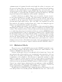
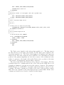
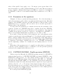
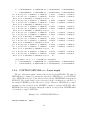
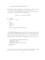
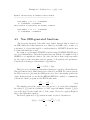
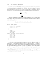
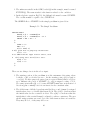
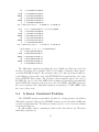
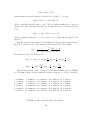
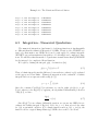
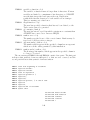
For this brief discussion on global errors, we solve a simple second-order nonlinear
periodic ODE and plot the absolute errors against time. This problem was first solved
in Reference 3.
df
d2 f
= −f − f, with f (0) = 0 and f˙(0) = 3.
2
dt
dt
7
·
··
··
····
·····
·
·
·
·
·
·
·
DVERK ····
·
··
··
··· ··· ···· ···
···· ····
·· ····
-8· ··
·
·
······
·
·
·
· ····· · · · · ·
··· ···
··
·· ·· ········ · ·· ···· ·· · · ·· ·· ·
··· ··· ········ ·· ··· ············· ·· ·· ···· ······ ······ ····· ······ ······
······
· ··
· · ·· · · · ·
··· ·
··· ···
··· ····
·
·
··· ···
·· ···
···· ··· ············ ··· ······ ······ ·····
·
·
·
·
·
·
·
·
·
··
·
·
·
·
·
·
·
·
·
·
··· ···
· ····
· ·
· ·
·
-9·
·
·
·
·
·
·
·
·
·
·
·
·
·
·
·
· ·
··
·
·· ·
·
···· ···· ···
·
·
··
·
·· · ···· ·
·
·
· ·
·
·
·
·
· ·
· ··
·
····
◦
· ·
·
·
◦
·
·
◦
◦
-10- ··
·
·
◦◦
◦
◦◦
·
◦◦
·
·
·◦
◦◦
◦◦ · ◦◦◦◦ ◦
◦
·
◦◦◦
◦◦
·◦ ◦
◦ ◦
···
◦
◦
◦
◦
◦◦
◦ ◦
·
◦ ◦◦
◦◦
◦
◦
-11-··
◦ ◦ · ◦◦◦ ◦
◦
◦
◦
◦
◦
◦
◦
◦
· ◦
◦◦
◦
ATOMFT
◦
◦
◦
-12◦
◦
◦
-130
time
50
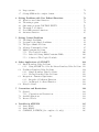
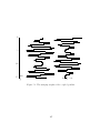
Figure 1.1: Global Error in Periodic Oscillation.
The absolute errors in the solution of this problem are shown in Figure 1. The
horizontal scale is time from zero to t = 50. The vertical scale is the logarithm of
the absolute error, log |ftrue − fcalc |. The upper curve in Figure 1 is the global error
in the solution by DVERK (a Runge-Kutta method) with a tolerance of 10−10 . The
bottom curve is the result from ATOMFT with the same error limit. These absolute
error values are obtained by comparison with a very precise calculation using an
extended-precision integer-math method.
The global error from ATOMFT is much smaller than the global error from
DVERK for the same error limit. This is indicative of the superior error control
under ATOMFT. The propagation of the global error over time can be seen by examining the plot for the DVERK results. (Since ATOMFT takes very large integration
steps, there are too few points for analysis.) The tops of the global error plot are on
the line for the square of the time. The magnitude of the global error for nonlinear
periodic oscillation increases quadratically with time.
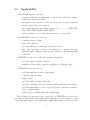
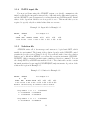
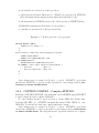
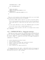
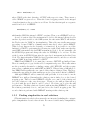
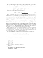
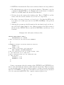
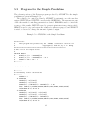
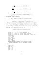
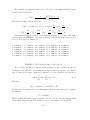
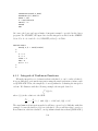
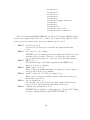
To study the cyclical behavior, we plot the phase diagrams for this problem.
Nonlinear problems have distinctively shaped phase diagrams. The usually shown
phase diagram is that for (f˙ vs f ). We are going to plot the phase diagram for (f¨ vs
8
f¨
·
···
·· ·· · ······
··
·
··
·
·
··
··
·· ·
·
··
·· ·
·
···
···
···
···
···
··
··
···
··
··
··
···
·· ··
·
··
··
··
··
·
··
··
·
··
·
··
··
···
··
···
·
······ ·· · ··
f˙
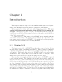
Figure 1.2: Phase diagram for f¨ vs f˙.
f˙), the derivatives. This is because we have discovered that the cyclical component
of the global error has a phase diagram with the same shape as the phase diagram
for (f¨ vs f˙).
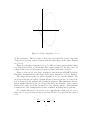
Figure 2 is the phase diagram for (f¨ vs f˙). This is a linear graph with the values
of f¨ vertical and values of f˙ horizontal. The origin is marked by the large circle. It
is shaped like a fan, and the points progress clockwise as the time advances.
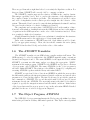
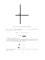
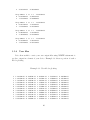
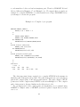
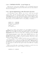
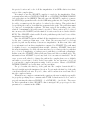
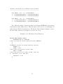
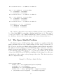
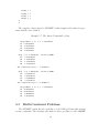
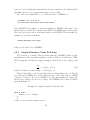
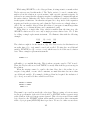
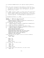
Figure 3 is the global error phase diagram for data from the ATOMFT solution.
This phase diagram has the same shape as the phase diagram for (f¨ vs f˙), Figure 2.
The shapes shown in the two phase diagrams above are basically similar. The
exception is that the error phase diagram (Figure 3) increases in size on each revolution as dictated by the quadratically growing propagation. This similarity in the two
shapes signifies that the global error is proportional to the derivative of the solution
function. We cannot prove this conclusion; we only offer the evidence. This similarity
is found in all of the examples that we have examined, including chaotic systems.
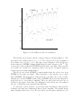
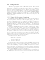
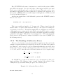
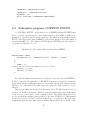
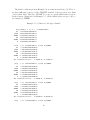
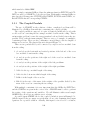
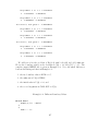
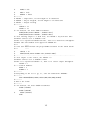
We continue this study of global errors by comparing the solutions to two problems, a two-body problem and a chaotic problem. The two-body problem has a period
of 2π.
x
d2 x
=− ,
2
dt
a
d2 y
y
=− ,
2
dt
a
9
f¨
·
· ·
·
·
·
· · ·
·
·
· ·
· ·····
·
·
·· · ·
·
· ·
· · ······· · · · ·
· ·
·
·· ············· ·
·
·· ·· ·········· ·· ·
·· ····················· · ·
·
f˙
·
·· ·· ··· ····· ·
·· ·· · ···· · · ·
····· ·········· ··· · ·
·
········· ···
·
·
·
·
·
· · ··
· ·· · · ·
· ·
· ·
··· · ··
·
·
·
· · ·
Figure 1.3: Error phase diagram (ATOMFT).
where a = (x2 + y 2 )3/2 . The initial values for x, y, ẋ, and ẏ are determined from
the eccentricity of the orbit, e, as follows
x(0) = 1 − e, ẋ(0) = 0, y(0) = 0,
and ẏ(0) =
(1 + e)1/2
.
(1 − e)1/2
We will use an eccentricity of e = 9.
Chaotic dynamical problems are particularly difficult to solve numerically. Many
chaotic problems have singularities in the complex plane that form natural boundaries
(6, 8, 9). Our example is the Henon-Heiles problem
d2 x
= −x − 2xy,
dt2
d2 y
= −y − x2 + y 2 ,
dt2
with initial conditions: x(0) = − 0.3225, y(0) = − 0.3532, ẋ(0) = 0.24943, and
ẏ(0) = 0.29403.
10
-1···
····
·
· ·
···············
·
Henon-Heiles ·· · ··
-3············
··· ·········· ···· · ··
············ · ·
-4··· ············· · ·· ·
··················· · ··
◦
·
·
-5two-body ◦ ◦ · ◦◦◦··◦ ·····◦·◦◦◦ ·◦◦◦◦◦ ◦◦◦◦◦ ◦◦◦◦◦◦ ◦◦◦◦◦◦◦◦ ◦◦◦◦
◦◦·· ··◦
◦
◦
·◦◦· ◦◦◦ ◦◦◦◦ ◦◦◦◦ ◦◦ ◦ ◦
◦
◦
◦◦· · ···◦
◦◦
◦
◦
◦
◦
◦
◦◦
◦
◦◦
◦◦·◦ ··
◦
· ◦·◦·◦◦◦ ◦◦ ◦◦ ◦◦◦◦·◦ ·◦◦◦◦ ◦◦ ◦◦◦ ◦◦ ◦◦ ◦◦◦
◦◦
◦◦
◦
◦◦ ◦◦ ◦◦ ◦◦◦◦
◦ ◦·· ◦◦·· ◦·◦◦◦ ◦·◦ ◦ ◦ ◦ ◦ ◦
◦
◦
◦
◦
◦
◦ ◦
-6- ◦◦◦◦ ◦◦◦◦◦◦◦◦ ◦◦ ◦◦◦ ◦◦◦◦◦◦ ◦◦ ◦◦ ◦ ···◦·◦···◦·◦···· ◦··◦·◦ ◦·◦ ◦◦ ◦ ◦◦ ◦◦
◦
◦
◦ ◦ · · ··
◦◦
◦◦
◦
◦◦
◦
◦
◦
·
◦
◦
◦
◦
◦
◦
·
◦
◦
·
·
◦
◦
◦
◦
·
·
·
◦◦ ··· ◦
·
◦ ◦◦ ◦ ◦ ◦ ◦ ◦ ◦◦
◦◦
· ······ ◦ ◦· ◦
◦
·· ··· ····· · ◦
-7- ◦◦◦ ◦ ◦ ◦ ◦◦
·
◦
◦
·
◦
·
◦
·
·
◦
·
◦
···· ··· ·
-8- ◦◦
······ ·········· · ·
◦
··· ·······
·
·
-9- ◦ ···· ··· ·· ······ ····
◦
· ·····
◦ ·· ·· · ···
· ·
◦ · ·· · ·
-10-◦◦··· ···· · ·
◦ ·
◦· ·
·
-11 ◦··· ·
◦··
·
-12- ·
0
95
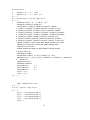
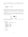
time
-2-
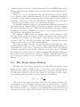
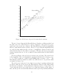
Figure 1.4: Global error for periodic versus chaotic systems.
The two-body problem and the Henon-Heiles problem have oscillations with about
the same period, 2π. This allows for a direct comparison of the global error propagation processes in the two solutions. The Henon-Heiles problem has singularities
that are 3 time units from the real axis. The two-body problem has singularities that
are only 0.03 time units from the real axis. A singularity’s distance from the real
axis is directly related to the radius of convergence. Therefore, the two-body problem
reguires stepsizes that are about one hundred times smaller than the Henon-Heiles
problem.
We show in Figure 4 the global errors for these two problems. The vertical scale
is the logarithm of the error magnitudes, and the horizontal scale is from t = 0 to
t = 95. These results are obtained from DVERK with a tolerance of 10−10 . The
Henon-Heiles results are marked by small dots, while the two-body problem results
are marked by larger dots.
The global error in the two-body solution is very large beginning with the first
revolution, while the global error in the Henon-Heiles solution is quite small during
the first few revolutions. As the numerical solutions progress to longer times, we
observe that the global error in the two-body solution propagates as the square of
time, and the global error in the Henon-Heiles solution grows exponentially with time.
11
The exponential propagation is the characteristic of a chaotic problem.
1.9
Purpose of the User Manual
This ATOMFT User Manual is designed to support easy, and efficient use of the
ATOMFT system. Chapter 2 can be used as a tutorial. The rest of this User Manual
is written as a reference manual.
This user manual is written with many, many illustrative examples. The user
can find all the important information about ATOMFT by examining the
examples. Although it is possible to learn to use ATOMFT without reading the
detailed text, one should read the manual at least once through to get the full flavor
of this Taylor series method.
Chapter 1 presents an overview of the ATOMFT system to help you understand
how its components fit together. This information is helpful to using the system as
described in the rest of the manual. A more detailed discussion can be found in
references (4) and (6).
Chapter 2 is written as a tutorial for new users of the ATOMFT system. Its
purpose is to show you how to use the ATOMFT system to solve initial value problems
in ODEs. It assumes that you are familiar with Fortran programming and with the
concept of computing a solution to a system of ODEs. It gives examples showing how
to solve specific differential equations.
Chapter 3 is for users who already have some experience using the ATOMFT
system. This chapter is the heart of this User Manual. It shows you how to use each
of the features available from the ATOMFT translator and from the ATSPGM object
program. It is organized for reference, not for sequential reading.
Chapter 4 contains a detailed discussion on the use of ATOMFT to solve problems
with user defined functions. Chapter 5 discusses the use of ATOMFT to solve control
problems (DAEs). Chapter 6 contains discussions on the solution of linear and nonlinear two-point boundary-value problems, numerical integration (quadrature), and
time delay problems. All of these problems can be solved automatically by application
of the ATOMFT systdm.
In Chapter 7, we summarize the conventions which are followed when using the
ATOMFT system. It includes a list of the allowable mathematical functions which
may be used to state the ODEs, and a list of reserved words which may not be used
as variable names.
Chapter 8 contains a discussion of the variables used by ATSPGM so that a user
may modify them for solving a particular problem. Chapter 9 contains a description
of the installation procedure. Chapter 10 contains a list of the messages which may
be produced by the ATOMFT translator.
Appendix A is a listing of the MAIN program of ATOMFT. In Appendix B, we
discuss the creation and formation of the RDCV subroutine library for ATOMFT.
12
1.10
Acknowledgements
The author would like to express his gratitude to Roy Morris for the initial design
and coding of the translator program, to John Fauss, David Lowery, and Manuel
Prieto for their work on series analysis, to Ray Moore, Mike Tabor, John Weiss for
many helpful suggestions, to R. Stanford, P. Breckheimer, and K. Berryman at Jet
Propulsion Labs for requesting user defined functions, and to Jon Wright for the
many bugs found. In particular, he gives thanks to Professor George Corliss for joint
research on Taylor series.
1.11
bibliography
(1) D. Barton, I. M. Willers, and R. V. M. Zahar. The automatic solution of ordinary
differential equations by the method of Taylor series. Comput. J. 14, 1971, pp 243-248.
(2) Kenneth W. Berryman, Richard H. Stanford, and Peter J. Breckheimer. The
ATOMFT integrator: Using Taylor series to solve ordinary differential equations.
AIAA J. 88-4217-CP, 1988, p55.
(3) Y. F. Chang. Automatic solution of differential equations. In Constructive and
Computational Methods for Differential and Integral Equations, edited by D. L. Colton
and R. P. Gilbert, Springer Lecture Notes in Math. ,vol. 430, Springer-Verlag, New
York, 1974, pp. 61-94.
(4) Y. F. Chang, J. Fauss, M. Prieto and George Corliss. Convergence analysis of
compound Taylor series. In Proceedings of the Seventh Conference on Numerical
Mathematics and Computing. University of Manitoba, 1978, pp. 129-152.
(5) Y. F. Chang and George Corliss. Ratio-like and recurrence relation tests for
convergence of series. J. Inst. Math. Appl, 25, 1980, pp. 349-359.
(6) Y. F. Chang, M. Tabor, J. Weiss, and G. Corliss. On the analytic structure of
the Henon-Heiles system. Phys. Lett. 85A (1981), pp. 211-213.
(7) Y. F. Chang and George Corliss. Solving ordinary differential equations using
Taylor series. ACM Trans. Math. Soft. 8, 1982, pp. 114-144.
(8) Y. F. Chang, M. Tabor, and J. Weiss. Analytic structure of the Henon-Heiles
Hamiltonian in integrable and nonintegrable regions. J. Math. Phys. 23(4), 1982,
pp. 531-538.
(9) Y. F. Chang, J. M. Greene, M. Tabor, and J. Weiss. The analytic structure of
dynamical systems and self-similar natural boundaries. Physica 8D. 1983, pp 183-207.
(10) Y. F. Chang. The ATOMCC Toolbox. BYTE. April, 1986, pp. 215-224.
(11) Y. F. Chang and George Corliss. Solving Control Problems with Multiple Constraints. In Proc. 13th IMACS World Congress, R. Vichnevetshi and J. J. H. Miller
13
(Eds), 1991, pp. 1331-1332.
(12) Y. F. Chang. ATOMFT USER MANUAL, Version 3.11. March, 1993.
(13) George Corliss and D. Lowery. Choosing a stepsize for Taylor series methods for
solving ODEs. J. Comput. Appl. Math. 3, 1977, pp. 251-256.
(14) George Corliss. Integrating ODEs in the complex plane - Pole vaulting. Math.
Comp. 35, 1980, pp. 1181-1189.
(15) George Corliss and Y. F. Chang. G–Stop facility in ATOMFT, a Taylor series
ODE solver. In Computational ODE, edited by S. O. Fatunla, University of Benin,
Benin-City, Nigeria, 1990, pp. 37-77.
(16) R. E. Moore. Interval Analysis. Prentice-Hall, Englewood Cliffs, N. J., 1966.
(17) L. B. Rall. Automatic Differentiation: Techniques and Applications. Springer
Lecture Notes in Computer Science, vol. 120, Springer-Verlag, Berlin, 1981.
14
Chapter 2
New Users
This Chapter is written for new users of the ATOMFT system. It shows you how
to solve initial value problems in ordinary differential equations using ATOMFT. We
give specific examples of how to solve ODEs. Detailed explanations of individual
features of ATOMFT are given in Chapter 3. Installation instructions can be found
in Chapter 9 and Appendix B.
*** W A R N I N G *** This version 3.11 of ATOMFT is not compatible with
any of its earlier versions. Therefore, you are a new user even if you have used a
previous version of ATOMFT.
2.1
Task of the ATOMFT Translator
The ATOMFT system is a tool to solve differential equations. It consists of
two major components: a translator program (ATOMFT), and a subroutine library
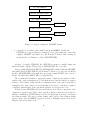
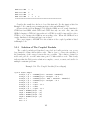
(RDCV). To understand the operation of these two components, you must first understand the six steps involved in using the system (see Figure 2.1). We discuss
the purpose of each step briefly to acquaint you with the terms used in the detailed
discussion in the section [Using the ATOMFT system].
At Step 1 (edit ODEINP), the system of differential equations are stated in a
form acceptable to ATOMFT. The input file ODEINP contains four separate blocks.
The first block contains the differential and algebraic equations. ATOMFT compiler
processes the data in this block to produce a Fortran object program ATSPGM which
is then compiled and executed to solve the problem. The second, third, and fourth
blocks are copied unchanged from ODEINP to predetermined locations in ATSPGM.
At Step 2 (run ATOMFT), ATOMFT
1. reads the first block from ODEINP,
2. analyzes the differential equations,
3. generates the ATSPGM program, and
15
#1 edit ODEINP
#2 run ATOMFT.EXE
#3 compile ATSPGM
(RDCV.LIB)
#4 link ATSPGM & RDCV
#5 data file
#6 run ATSPGM.EXE
Figure 2.1: Steps for using the ATOMFT system.
4. copies the second, third, and fourth blocks from ODEINP directly into
ATSPGM at locations shown by examples below. (You must have previously
compiled ATOMFT and linked it to the Fortran-77 library; thus creating an
executable file, see Chapter 9; call it ATOMFT.EXE.)
At Step 3 (compile ATSPGM), the ATSPGM program is compiled using any
suitable Fortran compiler. This produces ATSPGM.OBJ; the object file.
At step 4 (link ATSPGM & RDCV), ATSPGM.OBJ is linked with the ATOMFT
subroutine library RDCV.LIB and the Fortran-77 library to produce an executable
module, ATSPGM.EXE. (You must have previously compiled RDCV and created a
library. We shall call it RDCV.LIB, see Appendix B.)
The recommended manner to supply the initial conditions, the interval of integration, and control parameters is to read them from a data file which you prepare
at Step 5. The format of this data file is completely under your control as shown by
examples below. Step 5 may be done at any time before Step 6, or it may be omitted
completely. Initial values of the dependent variables are now preset to zero.
At Step 6 (run ATSPGM), the given problem is solved. Every component of the
equations is expanded in a Taylor series, and the solution point is moved forward by
analytic continuation. ATSPGM may read the data file prepared at Step 5 and writes
the solution results. The exact content, format, and location of the solution results
depend on the data in ODEINP prepared at Step 1. Examples given below and in
Chapter 3 show how this is done.
16
2.2
Using the ATOMFT system
In this section, we take you step-by-step through an example using the ATOMFT
system.
2.2.1
Step 1 - edit ODEINP
The input file ODEINP (ODEINP.
ATOMFT
in some operating system)specifies for
1. the system of differential equations to be solved,
2. how the initial conditions and the interval of integration are communicated to
ATSPGM, and
3. the commands to control the operation of ATOMFT or to control the execution
of ATSPGM.
The statements in ODEINP follow Fortran conventions. A “C” in column 1 denotes a COMMENT, columns 1-5 are used for label numbers, column 6 is used for
continuation, columns 7-72 contain statements, and columns 73-80 are ignored. The
statements in ODEINP may be in either upper case or lower case letters. In our
discussions in this Manual, we use upper case letters for emphasis. Important note:
Label numbers below 100 and above 999 are reserved for ATOMFT; so, the user can
only use the label numbers 100 through 999. Caution: ATOMFT does not recognize
the tab character.
Example 2-1. Simple ODEINP file.
C First Painleve transcendent
DIFF(Y,T,2) = 6*Y*Y + T
$
$
MSTIFF = 1
OPEN(1,FILE=’DATA’)
C Read integration interval and initial conditions.
READ(1,110) START,END,Y(1),Y(2)
110 FORMAT(4F10.3)
WRITE(LIST,120) START,END,Y(1),Y(2)
120 FORMAT(’ Solve first Painleve transcendent’ /
A ’ interval:
’,2F10.3 /
A ’ initial conditions:’,2F10.3 /)
$
$
17
In the Example 2-1, the MSTIFF=1 option (for infinite-series method) is invoked.
For illustrative purposes, all the examples in this manual will use this option whenever
possible. It is for illustration only; its precision may be in doubt. Under the normal
operating condition, ATOMFT controls the local truncation error to be very close
to the error limit set by the user. When MSTIFF=1 is invoked, the accuracy of the
results obtained may not be within the error limit as set by the user.
ODEINP must contain four blocks. Each block must terminate with the block
terminator “$” in columns 2-72. Blocks 2 and 4 are empty in Example 2-1.
The first block contains the system of differential equations. These equations are
processed by ATOMFT to determine the recursion relations that are written into
ATSPGM to generate the Taylor series for each component of the solution. To enter
the differential equations, DIFF(Y,T,N) denotes the N-th derivative of Y with respect
to T. N may range from 0 to 8, inclusively. The DIFF(,,) function is used to specify
the system of ODEs with Fortran-like statements using standard Fortran operators
and functions.
Under rare circumstances, ATOMFT may fail to produce the correct ATSPGM
for your problem. If it does fail, run COPTION DUMP=6 (see Section 3.2.7), and
send a copy of the output to Y. F. Chang at the address on the front cover.
The first block can also be used to control the operation of ATOMFT. The most
commonly used option is for ATOMFT to write ATSPGM in double-precision. For
this, use a “COPTION DOUBLE” card at the beginning of block 1.
Example 2-2. Double precision ATSPGM.
COPTION DOUBLE,DUMP=1
C First Painleve transcendent
DIFF(Y,T,2) = 6.0*Y*Y + T
$
$
MSTIFF = 1
OPEN(1,FILE=’DATA’)
C Read integration interval and initial conditions.
READ(1,110) START,END,Y(1),Y(2)
110 FORMAT(4F10.3)
WRITE(LIST,120) START,END,Y(1),Y(2)
120 FORMAT(’ Solve first Painleve transcendent’ /
A ’ interval:
’,2F10.3 /
A ’ initial conditions:’,2F10.3 /)
$
$
18
The second block is usually empty. It is used to insert non-executable Fortran
statements such as a SUBROUTINE card, a DIMENSION card, a COMMON card,
etc. at the beginning of ATSPGM.
The second, third, and fourth blocks are not processed syntactically by ATOMFT;
they are copied directly from ODEINP into ATSPGM. Example 2-3 is the ATSPGM
program written by ATOMFT for the ODEINP file shown in Example 2-1. Notice
where block 3 is copied into ATSPGM.
The third block is used to specify the interval of integration and the initial conditions by reading them from a data file prepared at Step 5. This is the file DATA
opened in block 3. The interval of integration is from START to END. END can
be less than START for integration in a negative direction. The initial values (at
START) of a dependent variable named y and its derivatives are assigned to the
array Y as follows:
Y(1) denotes y at START,
Y(2) denotes y’ at START,
Y(3) denotes y’’ at START, etc.
Thus, in Example 2-1, two initial conditions Y(1) for y(0) and Y(2) for y’(0) are
entered for the second order differential equation. Initial values of the dependent
variables are now preset to zero. This is done for the benefit of those (this author)
wishing to save typing a line for the input when it is zero.
All other valid Fortran statement may be included in block 3 to be copied into
ATSPGM, as shown in Example 2-1 by the WRITE statement to echo the input.
Label numbers below 100 and above 999 are reserved for ATOMFT. The third block
may also be used to change the default values of method-controlling variables. You
can see in Example 2-3 that many variables are initialized before and after block 3.
The meanings of these variables are described in Chapter 3.
The fourth block is usually empty. It may be used to insert statements into
ATSPGM at the end of each integration step.
This concludes the discussion of how to prepare the input file. More information
about the use of specific features can be found in Chapter 3.
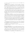
Example 2-3. ATSPGM for Example 2-1.
C*+*+*+*+*+*
C
This program was produced by the ATOMFT translator version 3.11
C
Copyright(c) 1979-93, by Y. F. Chang
C*+*+*+*+*+*+*+*+*+*+*+*+*+*+*+*+*+*+*+*+*+*+*+*+*+*+*+*+*+*+
C This is for the inputs below.
19
C First Painleve transcendent
C
DIFF(Y,T,2) = 6*Y*Y + T
C-------C no instructions in Second input block
C-------DIMENSION TMPS( 39, 1),TMPV( 40)
DIMENSION IPASS(20),RPASS(20)
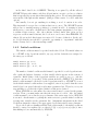
EQUIVALENCE (IPASS(1),NUMEQS),(IPASS(2),LENSER),
A (IPASS(3),LENVAR),(IPASS(4),MPRINT),(IPASS(5),LIST),
A (IPASS(6),MSTIFF),(IPASS(7),LRUN),(IPASS(8),KTRDCV),
A (IPASS(9),KNTSTP),(IPASS(10),KTSTIF),(IPASS(11),KXPNUM),
A (IPASS(12),KDIGS),(IPASS(13),KENDFG),(IPASS(14),NTERMS),
A (IPASS(15),KOVER),(RPASS(1),RADIUS),(RPASS(2),H),
A (RPASS(3),HNEW),(RPASS(4),ERRLIM),(RPASS(5),ADJSTF),
A (RPASS(6),XPRINT),(RPASS(7),DLTXPT),(TMPS(1,1),TMPV(1))
A,(RPASS(8),START),(RPASS(9),END),(RPASS(10),ORDER)
CHARACTER*6 NAMES
EQUIVALENCE (TMPS(1,1),Y(1))
DIMENSION NAMES(2), Y(39), T(2), TMPAAB(30), TMPAAA(30)
DATA NAMES(1)/’
T’/
DATA NAMES(2)/’
Y’/
Y(34) = 2.21
C-------C Initialize variables to default values.
C-------NTERMS = 2
NSTEPS = 40
MPRINT = 4
LIST = 0
DETUNE = 1.0
NUMEQS = 1
LENVAR = 39
ERRLIM = 1.E- 6
LENSER = 30
KTRDCV = 2
ADJSTF = 1.E-2
H = 1.4131E0
START = 0.E0
END = 0.E0
MSTIFF = 0
KENDFG = 3
LRUN = 1
KXPNUM = 3070038
KDIGS = 6
CALL HEAD(5,TMPV,NAMES,IPASS,RPASS)
20
DLTXPT = 0.E0
C-------C start of Third input block
C-------MSTIFF = 1
OPEN(1,FILE=’DATA’)
C Read integration interval and initial conditions.
READ(1,110) START,END,Y(1),Y(2)
110 FORMAT(4F10.3)
WRITE(LIST,120) START,END,Y(1),Y(2)
120 FORMAT(’ Solve first Painleve transcendent’ /
A ’ interval:
’,2F10.3 /
A ’ initial conditions:’,2F10.3 /)
C-------C end of Third input block
C-------NUMEQS = 1
LENVAR = 39
KOVER = 1
CALL HEAD(1,TMPV,NAMES,IPASS,RPASS)
C More initializations
C-------DLTXPT = SIGN(DLTXPT,(END-START))
H = SIGN(H,(END-START))
XPRINT = START + DLTXPT
LRUN = 1
KTSTIF = 0
IF(LENSER.GT.(LENVAR- 9)) LENSER = LENVAR - 9
C-------C Loop for integration steps. Inside the loop, print the desired output
C-------17 DO 27 KINTS=1,NSTEPS
KNTSTP = KINTS
19 CONTINUE
T(1) = START
T(2) = H
Y(2) = Y(2)*(H)
C-------C Preliminary series calculations
C-------TMPAAA(1) = 6.E0*Y(1)
TMPAAB(1) = TMPAAA(1)*Y(1)
Y(3) = (TMPAAB(1) + T(1))*(H*H/2.E0)
TMPAAA(2) = 6.E0*Y(2)
TMPAAB(2) = TMPAAA(1)*Y(2) + TMPAAA(2)*Y(1)
21
Y(4) = (TMPAAB(2) + T(2))*(H*H/6.E0)
C-------C Loop for series calculations
C-------DO 23 K= 5,LENSER
KA = K - 1
KB = K - 2
KC = K - 3
KD = K - 4
TMPAAA(KB) = 6.E0*Y(KB)
TMPAAB(KB) = 0.E0
KZ = 1 + KB
DO 1000 N=1, KB
L = KZ - N
TMPAAB(KB) = TMPAAB(KB) + TMPAAA(N)*Y(L)
1000 CONTINUE
Y(LENVAR) = (K)
Y(K) = (TMPAAB(KB))*(H*H/(KB*KA))
C-------C Test and adjust H to avoid over/under flow.
C-------CALL HEAD(2,TMPV,NAMES,IPASS,RPASS)
IF(LRUN.EQ.0) GO TO 19
23 CONTINUE
C-------C Calculate radius of convergence and take optimum step.
C-------CALL RDCV(TMPV,NAMES,IPASS,RPASS)
24 CALL RSET(TMPV,NAMES,IPASS,RPASS)
C-------C no instructions in Fourth input block
C-------25 GO TO (26,28,24), KENDFG
26 H = SIGN(RADIUS,H)*DETUNE
START = START + HNEW
27 CONTINUE
CALL HEAD(3,TMPV,NAMES,IPASS,RPASS)
28 CONTINUE
29 STOP
END
22
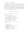
2.2.2
Step 2 - Run ATOMFT
The appropriate command to execute the ATOMFT compiler is [RUN ATOMFT],
or simply [ATOMFT]. The ATOMFT translator uses two files: ODEINP for the input
equation statements and initial conditions, and ATSPGM for the output object program. The messages produced by ATOMFT are placed on your terminal. Notice that
the important computer parameters are now calculated automatically by ATOMFT.
This information is placed on the terminal every time ATOMFT is executed. If you
should desire not to see this information, you must add a COPTION DUMP=1 line
at the beginning of you ODEINP file. (The CDC and Cray computers require the
user to specify either DUMP=8 or DUMP=9.)
Example 2-4. Translator messages for (2-1).
ATOMFT ver. 3.11, copyright(C) 1979-93, Y. F. Chang
--------------------------------------------------C First Painleve transcendent
SINGLE-precision mantissa has 24 binary bits,
round-off error
5.96E-08
minimum guaranteed error
1.19E-07
SINGLE-precision max value, 10**(
38), approx.
The real number unit is 32 binary bits long.
DOUBLE-precision mantissa has 53 binary bits,
round-off error
1.11E-16
minimum guaranteed error
2.22E-16
DOUBLE-precision max value, 10**( 307), approx.
DIFF(Y,T,2) = 6*Y*Y + T
$
$
MSTIFF = 1
OPEN(1,FILE=’DATA’)
C Read integration interval and initial conditions.
READ(1,110) START,END,Y(1),Y(2)
110 FORMAT(4F10.3)
WRITE(LIST,120) START,END,Y(1),Y(2)
120 FORMAT(’ Solve first Painleve transcendent’ /
A ’ interval:
’,2F10.3 /
A ’ initial conditions:’,2F10.3 /)
$
$
23
In the normal usage of the ATOMFT system, it is not necessary for the user to
inspect the code in ATSPGM. However, in the event of an error or if some small
changes are desired, the user can edit ATSPGM by hand.
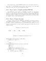
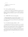
2.2.3
Step 3 and 4 - Compile and link ATSPGM
The ATSPGM program, written by ATOMFT, is just like any other Fortran
program; you may edit it to suit your needs. Whether edited or not, ATSPGM is
ready to be compiled and linked with the subroutine library (RDCV.LIB). (The name
for this library may be different on your computer system.) Please read Appendix B
for examples of how to create this library file.
2.2.4
Step 5 - Prepare the data
At Step 1, when you prepared ODEINP for ATOMFT, you may have included
some READ statements in block 3 to communicate the interval of integration and
the initial conditions to ATSPGM. Before you run ATSPGM, the data file to be read
by those statements must be prepared with the appropriate file name given in your
OPEN statement.
Example 2-5. Data file for (2-1).
0.000
1.100
1.000
0.000]
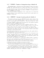
Example 2-6. Assignment statements, block 3.
COPTION DUMP=1 C First Painleve transcendent
DIFF(Y,T,2) = 6*Y*Y + T
$
$
MSTIFF = 1
C Assign integration interval \& initial conditions.
START = 0.0
END = 1.1
Y(1) = 1.0
WRITE(LIST,120) START,END,Y(1),Y(2)
120 FORMAT(’ Solve first Painleve transcendent’ /
A ’ Interval:
’,2F10.3 /
A ’ Initial conditions:’,2F10.3 /)
24
$
$
If you know that you will be solving a simple problem only once, Step 5 can be
eliminated by stating the values of START, END, and the initial conditions with
Fortran assignment statements in block 3 as shown in Example 2-6.
2.2.5
Step 6 - Run ATSPGM
At step 6, you are ready to run ATSPGM. ATSPGM writes its output to the
logical unit LIST. You may assign that unit to a disk file, a printer, or a terminal.
This assignment is system dependent. Perhaps the best thing to do is to declare an
OPEN(LIST,,,) statement in block 3.
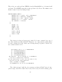
Example 2-7. Solution Output for Example 2-6.
Solve the first Painleve transcendent
interval:
0.000
1.100
initial conditions:
1.000
0.000
Results calculated by an infinite-series method.
-----------------------------------------------Step number 0 at T = 0.00000E+00
Y 1.00000E+00 0.00000E+00
This solution is limited by the machine roundoff.
Step number 1 at T = 6.30000E-01
Y 3.00802E+00 1.03304E+01
Step number 2 at T = 1.10000E+00
Y 8.77740E+01 1.64472E+03
The output is given in Example 2-7. There are two extra lines of information
as compared to previous versions of ATOMFT. One line informs you that the MSTIFF=1 option (for infinite-series method) is operative. The other line informs you
that the pre-set error limit used (1.E-6) is either equal to, or very close to, the machine
roundoff. This message is given only when the infinite-series method is used.
You may find it helpful to write a command file to help you run ATOMFT. That
would be a xxx.COM in VAX/VMS, a xxx.BAT in MS/DOS, or a shell script in
UNIX. Examples can be found in Appendix D.
25
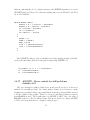
2.3
Output at equally spaced points
Now, you should be able to use ATOMFT to solve routine problems. The points
at which ATSPGM computes the solutions are determined by the actual integration
steps taken which are not uniform in size. This Section shows you how to force
ATSPGM to print the solutions at equally spaced points.
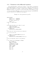
Example 2-8. Equally spaced output points.
COPTION DUMP=1
C First Painleve transcendent
DIFF(Y,T,2) = 6*Y*Y + T
$
$
MSTIFF = 1
MPRINT = 2
DLTXPT = 0.2
START = 0.0
END = 1.1
Y(1) = 1.0
WRITE(LIST,120) START,END,Y(1),Y(2)
120 FORMAT(’ Solve first Painleve transcendent’/
A ’ Interval:
’,2F10.3/
A ’ Initial conditions:’,2F10.3/)
$
$
The output from ATSPGM is controlled by two variables, MPRINT (amount of
print), and DLTXPT (print interval). To produce output at equally spaced points,
assign MPRINT=2 to turn off the print at the actual integration steps, and assign
DLTXPT=DELTA, where DELTA is your desired print interval. In Example 2-8, we
show a printing step of 0.2.
Example 2-9. Solution Output for Example 2-8.
Solve first Painleve transcendent
Interval:
0.000
1.100
Initial conditions:
1.000
0.000
Results calculated by an infinite-series method.
------------------------------------------------
26
Step number 0 at T = 0.00000E+00
Y 1.00000E+00 0.00000E+00
This solution is limited by the machine roundoff.
Step number 1 at T = 2.00000E-01
Y 1.12637E+00 1.32292E+00
Step number 1 at T = 4.00000E-01
Y 1.58305E+00 3.49159E+00
Step number 1 at T = 6.00000E-01
Y 2.72125E+00 8.83744E+00
Step number 2 at T = 8.00000E-01
Y 6.03835E+00 2.97144E+01
Step number 2 at T = 1.00000E+00
Y 2.33937E+01 2.26373E+02
Step number 2 at T = 1.10000E+00
Y 8.77740E+01 1.64472E+00
27
28
Chapter 3
How to Use the Options
This Chapter is written for users who already have solved several problems using
the ATOMFT system. It assumes familiarity with Fortran programming, with Chapter 2, and with the numerical solution of ODEs. This Chapter is the heart of this
User Manual.
*** W A R N I N G *** This version 3.11 of ATOMFT is not compatible with any
of its earlier versions. Many of the instructions are different, also. If you have experience using a previous version of ATOMFT, do be careful and read the appropriate
sections of this User’s Manual before executing ATOMFT.
This chapter is organized for reference, not for sequential reading. As a consequence, some information found in other parts of this Manual are repeated here,
possibly several times. There are many illustrative examples. The user can find all
the important information about ATOMFT by examining the examples.
All the options and method parameters available to the user are described in this
chapter. The applications of some of the parameters to specific types of problems are
discussed in Chapters 4, 5, and 6.
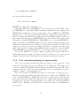
3.1
Solving your problem
The tasks which must be accomplished in order to run the ATOMFT system
on your computer were discussed in Chapter 2, in the section [Using the ATOMFT
system]. They are:
Edit ODEINP containing ODEs.
Run ATOMFT.EXE.
This creates ATSPGM, the Fortran
program. ATSPGM may be edited.
Compile ATSPGM.
29
This creates ATSPGM.OBJ.
Link ATSPGM.OBJ, with RDCV.LIB.
This creates ATSPGM.EXE.
Edit DATA input-file, if any.
Run ATSPGM.EXE
The specific file names are system dependent. We have given them names that
are more-or-less generic.
3.1.1
Translator file, ODEINP
The ODEINP file contains statements for the ODEs to be solved and information
specifying how the initial conditions and the integration interval are determined in
ATSPGM. It may contain commands to control:
1. the operation of the ATOMFT translator,
2. the execution of the solution, and
3. the desired format of the output.
The names ODEINP and ATSPGM are fixed within ATOMFT. These names
can be changed by changing the ATOMFT source codes in the MAIN program, see
Appendix A.
The data in ODEINP follows Fortran conventions. Columns 1-5 are used for
line numbers, column 6 is used for continuation characters, columns 7-72 contain
statements, and columns 73-80 are ignored. As in Fortran, all blanks are ignored.
A “C” in column 1 denotes a comment which is copied directly into the ATSPGM
file. The statements in ODEINP can be either upper case or lower case letters. (The
Fortran compiler that you are using may dictate your choice of case.) We use upper
case in this manual for emphasis. Important Note: Label numbers below 100 and
above 999 are reserved for ATOMFT. CAUTION: ATOMFT does not recognize
the tab character.
The ODEINP file contains four blocks. Each block ends with the block terminator
symbol “$” in columns 2-72. Each of the blocks is discussed in detail in this chapter.
Example 3-1 is an ODEINP file that shows several of the features which will be
discussed in later sections.
If you have a simple problem which is to be solved only once, the contents of the
“DATA” file may be entered directly as data into block 3. However, the repeated
compilation and linking of the ATSPGM file can take some time, so it is best to use
a data file on problems that are solved more than once.
30
Example 3-1. ODEINP file.
C Block 1
C
C System with parameter.
C
DIFF(X,T,2) = - ALPHA*X*R
DIFF(Y,T,2) = - ALPHA*Y*R
R = (X*X + Y*Y)**(-1.5)
ALPHA = 0.65
$
C Block 2
CHARACTER*80 LINE
$
C Block 3
C
C Read: heading line, print code, maximum number of integration
C
steps.
C Echo the above.
C Read: heading line, integration interval, print interval,
C
parameter in equations, initial conditions.
C Echo the above.
OPEN(1,FILE=’DATA’)
OPEN(7,FILE=’PLOTS’,STATUS=’NEW’)
READ(1,110) LINE,MPRINT,NSTEPS
110 FORMAT(A80/2I10)
WRITE(LIST,110) LINE,MPRINT,NSTEPS
READ(1,120) LINE,START,END,DLTXPT,ALPHA,X(1),X(2),Y(1),Y(2)
120 FORMAT(A80/8F10.3)
WRITE(LIST,120) LINE,START,END,DLTXPT,ALPHA,X(1),X(2),Y(1),Y(2)
C Assignment statements for the error control parameter
MSTIFF = 1
ERRLIM = 1.0E-04
$
C Block 4
C
C Produce file of data for plotting.
IF(KENDFG.EQ.3)WRITE(7,130)KINTS,XPRINT,X(31),X(32),Y(31),Y(32)
130 FORMAT(I2,1P5E13.5)
$
31
3.1.2
Translator file, the terminal
The translator messages contain information which the ATOMFT expects you
to inspect. The messages will appear on your terminal unless you have directed the
output to a file. It includes an echo of the input file and any error messages. Chapter
10 contains a list of the error messages and explanations so that you may correct your
input if necessary. Notice that the important computer parameters are now calculated
automatically by ATOMFT. This information is placed on the terminal every time
ATOMFT is executed. If you should desire not to see this information, you must add
a COPTION DUMP=1 line at the beginning of you ODEINP file. (The CDC and
Cray computers require DUMP=8 or DUMP=9.)
Example 3-2. Translator messages for Example 3-1.
ATOMFT ver. 3.11, copyright(C) 1979-93, Y. F. Chang.
----------------------------------------------------C Block 1
C
C System with parameter.
C
{\em SINGLE-precision mantissa has 24 binary bits,
round-off error
5.96E-08
minimum guaranteed error
1.19E-07
SINGLE-precision max value, 10**(
38), approximately.
The real number unit is 32 binary bits long.
DOUBLE-precision mantissa has 53 binary bits,
round-off error
1.11E-16
minimum guaranteed error
2.22E-16
DOUBLE-precision max value, 10**( 307), approximately.}
DIFF(X,T,2) = - ALPHA*X*R
DIFF(Y,T,2) = - ALPHA*Y*R
R = (X*X + Y*Y)**(-1.5)
ALPHA = 0.65
$
C Block 2
CHARACTER*80 LINE
$
C Block 3
C
C Read: heading line, print code, maximum number of integration
C
steps.
C Echo the above.
32
C
C
C
Read: heading line, integration interval, print interval,
parameter in equations, initial conditions.
Echo the above.
OPEN(1,FILE=’DATA’)
OPEN(7,FILE=’PLOTS’,STATUS=’NEW’)
READ(1,110) LINE,MPRINT,NSTEPS
110 FORMAT(A56/2I7)
WRITE(LIST,110) LINE,MPRINT,NSTEPS
READ(1,120) LINE,START,END,DLTXPT,ALPHA,X(1),X(2),Y(1),Y(2)
120 FORMAT(A56/8F7.3)
WRITE(LIST,120) LINE,START,END,DLTXPT,ALPHA,X(1),X(2),Y(1),Y(2)
C Assignment statements for the error control parameter
MSTIFF = 1
ERRLIM = 1.0E-04
$
C Block 4
C
C Produce file of data for plotting.
IF(KENDFG.EQ.3)WRITE(7,130)KINTS,XPRINT,X(31),X(32),Y(31),Y(32)
130 FORMAT(I2,1P5E13.5)
$
3.1.3
Translator file, ATSPGM
The ATSPGM file contains the Fortran object program written by ATOMFT to
solve the system of differential equations using long Taylor series. ATOMFT uses the
variable names given in ODEINP, so that ATSPGM appears to have been custom
written for the specific problem. Usually you do not need to inspect ATSPGM, but
sometimes you may wish to edit ATSPGM to suit your particular need.
Example 3-3. ATSPGM for Example 3-1.
C*+*+*+*+*+*
C
This program was produced by the ATOMFT translator version 3.11
C
Copyright(c) 1979-93, by Y. F. Chang
C*+*+*+*+*+*+*+*+*+*+*+*+*+*+*+*+*+*+*+*+*+*+*+*+*+*+*+*+*+*+
C This is for the inputs below.
C
C Block 1
C System with parameter.
C
C
DIFF(X,T,2) = - ALPHA*X*R
33
C
DIFF(Y,T,2) = - ALPHA*Y*R
C
R = (X*X + Y*Y)**(-1.5)
C
ALPHA = 0.65
C-------C start of Second input block
C-------C Block 2
CHARACTER*80 LINE
C-------C end of Second input block
C-------DIMENSION TMPS( 39, 2),TMPV( 79)
DIMENSION IPASS(20),RPASS(20)
EQUIVALENCE (IPASS(1),NUMEQS),(IPASS(2),LENSER),
A (IPASS(3),LENVAR),(IPASS(4),MPRINT),(IPASS(5),LIST),
A (IPASS(6),MSTIFF),(IPASS(7),LRUN),(IPASS(8),KTRDCV),
A (IPASS(9),KNTSTP),(IPASS(10),KTSTIF),(IPASS(11),KXPNUM),
A (IPASS(12),KDIGS),(IPASS(13),KENDFG),(IPASS(14),NTERMS),
A (IPASS(15),KOVER),(RPASS(1),RADIUS),(RPASS(2),H),
A (RPASS(3),HNEW),(RPASS(4),ERRLIM),(RPASS(5),ADJSTF),
A (RPASS(6),XPRINT),(RPASS(7),DLTXPT),(TMPS(1,1),TMPV(1))
A,(RPASS(8),START),(RPASS(9),END),(RPASS(10),ORDER)
CHARACTER*6 NAMES
EQUIVALENCE (TMPS(1,1),X(1)),(TMPS(1,2),Y(1))
DIMENSION NAMES(3), T(2), Y(39), R(30), X(39), TMPAAH(30),
A TMPAAG(30), TMPAAF(30), TMPAAE(30), TMPAAD(30), TMPAAC(30),
B TMPAAB(30)
DATA NAMES(1)/’
T’/
DATA NAMES(2)/’
X’/
DATA NAMES(3)/’
Y’/
X(34) = 2.21
Y(34) = 3.21
C-------C Constant expressions
C-------ALPHA = 6.5E-1
C-------C Initialize variables to default values.
C-------NTERMS = 2
NSTEPS = 40
MPRINT = 4
LIST = 0
DETUNE = 1.0
NUMEQS = 2
34
LENVAR = 39
ERRLIM = 1.E- 6
LENSER = 30
KTRDCV = 2
ADJSTF = 1.E-2
H = 1.4131E0
START = 0.E0
END = 0.E0
MSTIFF = 0
KENDFG = 3
LRUN = 1
KXPNUM = 3070038
KDIGS = 6
CALL HEAD(5,TMPV,NAMES,IPASS,RPASS)
DLTXPT = 0.E0
C-------C start of Third input block
C-------C Block 3
C
C Read: heading line, print code, maximum number of integration
C
steps.
C Echo the above.
C Read: heading line, integration interval, print interval,
C
parameter in equations, initial conditions.
C Echo the above.
OPEN(1,FILE=’DATA’)
OPEN(7,FILE=’PLOTS’,STATUS=’NEW’)
READ(1,110) LINE,MPRINT,NSTEPS
110 FORMAT(A80/2I10)
WRITE(LIST,110) LINE,MPRINT,NSTEPS
READ(1,120) LINE,START,END,DLTXPT,ALPHA,X(1),X(2),Y(1),Y(2)
120 FORMAT(A80/8F10.3)
WRITE(LIST,120) LINE,START,END,DLTXPT,ALPHA,X(1),X(2),Y(1),Y(2)
C Assignment statements for the error control parameter
MSTIFF = 1
ERRLIM = 1.0E-04
C-------C end of Third input block
C-------TMPAAA = -1.5E0
C-------C Constant expressions
C-------NUMEQS = 2
35
LENVAR = 39
KOVER = 1
CALL HEAD(1,TMPV,NAMES,IPASS,RPASS)
C More initializations
C-------DLTXPT = SIGN(DLTXPT,(END-START))
H = SIGN(H,(END-START))
XPRINT = START + DLTXPT
LRUN = 1
KTSTIF = 0
IF(LENSER.GT.(LENVAR- 9)) LENSER = LENVAR - 9
C-------C Loop for integration steps. Inside the loop, print the desired output
C-------17 DO 27 KINTS=1,NSTEPS
KNTSTP = KINTS
19 CONTINUE
T(1) = START
T(2) = H
X(2) = X(2)*(H)
Y(2) = Y(2)*(H)
C-------C Preliminary series calculations
C-------TMPAAB(1) = X(1)*X(1)
TMPAAC(1) = Y(1)*Y(1)
TMPAAE(1) = ALPHA*X(1)
TMPAAG(1) = ALPHA*Y(1)
TMPAAD(1) = TMPAAB(1) + TMPAAC(1)
R(1) = TMPAAD(1) ** TMPAAA
TMPAAF(1) = TMPAAE(1)*R(1)
X(3) = (-TMPAAF(1))*(H*H/2.E0)
TMPAAH(1) = TMPAAG(1)*R(1)
Y(3) = (-TMPAAH(1))*(H*H/2.E0)
TMPAAB(2) = X(1)*X(2) + X(2)*X(1)
TMPAAC(2) = Y(1)*Y(2) + Y(2)*Y(1)
TMPAAE(2) = ALPHA*X(2)
TMPAAG(2) = ALPHA*Y(2)
TMPAAD(2) = TMPAAB(2) + TMPAAC(2)
R(2) = TMPAAA*R(1)*TMPAAD(2)/TMPAAD(1)
TMPAAF(2) = TMPAAE(1)*R(2) + TMPAAE(2)*R(1)
X(4) = (-TMPAAF(2))*(H*H/6.E0)
TMPAAH(2) = TMPAAG(1)*R(2) + TMPAAG(2)*R(1)
Y(4) = (-TMPAAH(2))*(H*H/6.E0)
C--------
36
C Loop for series calculations
C-------DO 23 K= 5,LENSER
KA = K - 1
KB = K - 2
KC = K - 3
KD = K - 4
TMPAAB(KB) = 0.E0
TMPAAC(KB) = 0.E0
KZ = 1 + KB
DO 1000 N=1, KB
L = KZ - N
TMPAAB(KB) = TMPAAB(KB) + X(N)*X(L)
TMPAAC(KB) = TMPAAC(KB) + Y(N)*Y(L)
1000 CONTINUE
TMPAAE(KB) = ALPHA*X(KB)
TMPAAG(KB) = ALPHA*Y(KB)
TMPAAD(KB) = TMPAAB(KB) + TMPAAC(KB)
R(KB) = R(1)*TMPAAD(KC+1)*KC*TMPAAA
KY = 2 + KC
DO 1001 N=2, KC
L = KY - N
AL = (L - 1)
1001 R(KB) = R(KB) + R(N)*TMPAAD(L)*AL
A *TMPAAA - TMPAAD(N)*R(L)*AL
R(KB) = R(KB) /(KC)/TMPAAD(1)
TMPAAF(KB) = 0.E0
KZ = 1 + KB
DO 1002 N=1, KB
L = KZ - N
TMPAAF(KB) = TMPAAF(KB) + TMPAAE(N)*R(L)
1002 CONTINUE
X(LENVAR) = (K)
X(K) = (-TMPAAF(KB))*(H*H/(KB*KA))
TMPAAH(KB) = 0.E0
KZ = 1 + KB
DO 1003 N=1, KB
L = KZ - N
TMPAAH(KB) = TMPAAH(KB) + TMPAAG(N)*R(L)
1003 CONTINUE
Y(LENVAR) = (K)
Y(K) = (-TMPAAH(KB))*(H*H/(KB*KA))
C-------C Test and adjust H to avoid over/under flow.
C--------
37
CALL HEAD(2,TMPV,NAMES,IPASS,RPASS)
IF(LRUN.EQ.0) GO TO 19
23 CONTINUE
C-------C Calculate radius of convergence and take optimum step.
C-------CALL RDCV(TMPV,NAMES,IPASS,RPASS)
24 CALL RSET(TMPV,NAMES,IPASS,RPASS)
C-------C start of Fourth input block
C-------C Block 4
C
C Produce file of data for plotting.
IF(KENDFG.EQ.3)WRITE(7,130)KINTS,XPRINT,X(31),X(32),Y(31),Y(32)
130 FORMAT(I2,1P5E13.5)
C-------C end of Fourth input block
C-------25 GO TO (26,28,24), KENDFG
26 H = SIGN(RADIUS,H)*DETUNE
START = START + HNEW
27 CONTINUE
CALL HEAD(3,TMPV,NAMES,IPASS,RPASS)
28 CONTINUE
29 STOP
END
The Taylor series length for the independent variable is 2. The first term is
its value and the second term is the stepsize, H. The Taylor series length for the
dependent variables is 39. The Taylor series length for all auxiliary and temporary
variables is 30. The extra 9 terms are used by RDCV to store information about the
position of the primary singularity, its order, the accuracy of the calculation for the
radius of convergence, the length of the usable Taylor series, a pointer to the name
of the variable, an internal flag, and the initial conditions.
The series terms X(34) and Y(34) are the pointers to their names. The first
decimals in these two constants indicate the orders of the specific ODE. The second
decimals are dummies to prevent errors in real-to-integer conversion. The parameter
KXPNUM is used to warn RDCV of potential overflow. Its value is composed of two
constants. The upper constant above 1,000 is 9/10 of the double-precision overflow
limit. The lower constant is 9/10 of the single-precision overflow limit. All the other
constants and variables are described elsewhere in this chapter.
38
3.1.4
DATA input file
For most problems using the ATOMFT system, you should communicate the
initial conditions, the integration interval, the coefficients in the differential equations,
and the ATOMFT control parameters by reading them from a DATA input file. Initial
values of the dependent variables are now preset to zero. This means that you are
required to specify only those initial values that are non-zero.
Example 3-4. Input file for Example 3-1.
MPRINT
NSTEPS
4
80
START END
DLTXPT
1.000 10.000 0.250
3.1.5
for example 3-1
ALPHA
X(1)
0.580 -1.000
X(2)
0.000
Y(1)
0.000
Y(2)
4.300
Solution file
ATSPGM writes all of its messages and answers to logical unit LIST, which
usually is your terminal. The format of the solution depends on the ATOMFT control
parameters (see the section [Using block 3]). If you should wish to have the solution
written onto a disk file in MSDOS, you can use the execution statement (ATSPGM
PRTOUT). Other computer systems require a similar re-direction command. You can
also change LIST by an OPEN statement in block 3. The solution file can also contain
information written by user supplied WRITE(LIST,xxx) statements. A portion of the
solution file is given in Example 3-5.
Example 3-5. Solution for Example 3-1.
MPRINT
NSTEPS
for example 3-1
4
80
START END
DLTXPT ALPHA X(1) X(2) Y(1) Y(2)
1.000 10.000 0.250 0.580 -1.000 0.000 0.000 4.300
Results calculated by an infinite-series method.
-----------------------------------------------Step number 0 at T = 1.00000E+00
X -1.00000E+00 0.00000E+00
Y 0.00000E+00 4.30000E+00
Step number 1 at T = 1.23000E+00
X -9.87214E-01 9.52869E-02
39
Y
9.85352E-01
4.26058E+00
Step number 2 at T = 1.25000E+00
X -9.85268E-01 9.92470E-02
Y 1.07052E+00 4.25646E+00
Step number 2 at T = 1.50000E+00
X -9.56779E-01 1.23036E-01
Y 2.12958E+00 4.22039E+00
Step number 2 at T = 1.56000E+00
X -9.49326E-01 1.25304E-01
Y 2.38263E+00 4.21504E+00
Step number 3 at T = 1.75000E+00
X -9.25064E-01 1.29522E-01
Y 3.18223E+00 4.20277E+00
3.1.6
User files
It is often useful to create your own output files using WRITE statements to
produce output in a format of your choice. Example 3-6 shows a portion of such a
file for plotting.
Example 3-6. User file for plotting.
2
2
3
3
4
4
4
4
4
5
5
5
1.25000E+00
1.50000E+00
1.75000E+00
2.00000E+00
2.25000E+00
2.50000E+00
2.75000E+00
3.00000E+00
3.25000E+00
3.50000E+00
3.75000E+00
4.00000E+00
-9.85268E-01
-9.56779E-01
-9.25064E-01
-8.92334E-01
-8.59179E-01
-8.25811E-01
-7.92325E-01
-7.58767E-01
-7.25162E-01
-6.91527E-01
-6.57869E-01
-6.24196E-01
9.92470E-02
1.23036E-01
1.29522E-01
1.31981E-01
1.33132E-01
1.33748E-01
1.34111E-01
1.34338E-01
1.34489E-01
1.34592E-01
1.34665E-01
1.34718E-01
40
1.07052E+00
2.12958E+00
3.18223E+00
4.23159E+00
5.27901E+00
6.32515E+00
7.37039E+00
8.41497E+00
9.45905E+00
1.05027E+01
1.15461E+01
1.25891E+01
4.25646E+00
4.22039E+00
4.20277E+00
4.19295E+00
4.18678E+00
4.18258E+00
4.17953E+00
4.17723E+00
4.17543E+00
4.17398E+00
4.17279E+00
4.17180E+00
3.2
Using block 1
The first block contains the system of differential equations. These equations
are processed by ATOMFT to determine the recursion relations to be written into
ATSPGM to generate the Taylor series for each component of the solution. The first
block is also used for ATOMFT options to control the operation of the translator.
This is done by placing a COPTION card at the beginning of ODEINP. Multiple
translator options may be specified on the same line, i.e. COPTION DOUBLE,
LENVAR=40. Multiple COPTION cards are also allowed; they must precede all
other program cards.
3.2.1
Format for the system of equations
For differential equations, DIFF(Y,T,N) is used to denote the n-th derivative of
the dependent variable y with respect to the independent variable t. The value of
the variable N may range from 0 to 8, inclusively. The DIFF(Y,T,N) function is
used to specify ODEs just as with other standard Fortran operators and functions.
All functions supported by ATOMFT are listed in Chapter 7. The statements in
ODEINP can be either upper or lower case letters. We use upper case in this manual
for emphasis.
The input to ATOMFT follows Fortran conventions. Comment cards contain a
“C” in column 1. The entire comment card is reproduced in ATSPGM. Columns
1-5 are used to enter line numbers. Column 6 is used for continuation; there is a
limit of 19 continuation lines in Fortran. Columns 7-72 contain the statements of
the equations. Columns 73-80 are ignored. As in Fortran, blanks are not significant.
(A word of caution, the tab character is not recognized by ATOMFT.) ATOMFT
maintains a list of reserved words which may not be used as variable names in your
equations. All the reserved words are listed in Chapter 7.
The equations in block 1 must be of the form
or
DIFF(Y,T,N) = expression,
variable = DIFF(Y,T,N),
variable = expression.
An expression may contain operations on variables and DIFF(,,) functions. The
highest order derivative of each dependent variable must be given explicitly by an
equation of the form DIFF(,,) = expression, but DIFF(,,) functions of lower order may
appear in expressions on the right hand side. A system of differential equations may
not have more than one independent variable. For a problem with more independent
variables, use the function option described in Chapter 4.
Incidentally, ATOMFT transforms all constant integer powers of a variable up to 4
into multiplications. This is done in order to avoid the problems raised by the initial
41
value of that variable being equal to zero. For integer powers greater than 4, the
user is responsible to see that a l’Hopital situation does not arise. Except for integer
powers, constant coefficients which appear in ODEs are converted to real numbers
by ATOMFT, so that it does not matter whether three is written as 3, 3.0, 3.E0, or
3.D0.
3.2.2
Parameters in the equations
Example 3-1 shows a system involving parameters. It is often interesting to
explore the dependence of the solution on parameters which appear in the differential
equation. The ATOMFT system is especially well suited to this problem, because
ATSPGM needs to be generated only once and it can be executed repeatedly for
different values of the parameters.
You may enter the parameters as constants directly into the statement of the
equations. In that case, ATOMFT writes those constants directly into ATSPGM;
this approach does not allow easy modification of the parameters. Note that all
constants (except integer powers) are converted to real numbers by ATOMFT, so
that it does not matter whether three is written as 3, 3.0, 3.E0, or 3.D0.
If you wish to change the values of the parameters, give each parameter in the
equation a variable name as shown in Example 3-1. Note that the variable parameters
must be assigned dummy values in block 1, even though the actual values may be
specified at solution time by statements in block 3. The dummy values MUST NOT
be duplicates of any simple constants such as 0, 1, or 2. ATOMFT automatically
removes duplicating constants. Good numbers for the dummy values are: 0.1, 0.2,
0.3, etc.
If the values of the parameters are to be supplied at solution time by reading from
a data file or from a terminal, it may be convenient to solve the problem repeatedly
as shown by the example in the Subsection 3.4.3.
3.2.3
COPTION DOUBLE - Double-precision ATSPGM
Unless you specify differently, the ATSPGM program generated by ATOMFT is
written in single-precision. A COPTION DOUBLE card signals ATOMFT to write
ATSPGM in double-precision. No other changes should be made in block 1. In
particular, if the ODEs have library functions such as SIN, EXP, etc., ATOMFT
automatically inserts DSIN, DEXP, etc. into ATSPGM. You should not make those
substitutions yourself. We realize that many Fortran compilers no longer require the
addition of the “D”, “C”, or “Z” in front of these function names. However, we hold
the position that it is best to use them because it yields an additional opportunity to
check your program. For example, it may be important not to have a single-precision
value in a double-precision DSIN statement.
In a double-precision ATSPGM program,
42
• real variables are declared as double precision;
• double-precision Fortran functions (i.e. DLOG) are generated in ATSPGM;
(The user must still use single-precision functions in the first block.)
• call statements in ATSPGM reference the double-precision ATOMFT library;
• FORMAT statements use D-format for real variables;
• constants are generated in double-precision form.
Example 3-7. Double precision object program.
COPTION DOUBLE, DUMP=1
DIFF(Y,T,2) = 6*Y*Y + T
$
$
C Read initial conditions and integration interval
OPEN(1,FILE=’DATA’)
READ(1,110) START,END,Y(1),Y(2)
110 FORMAT(4F10.3)
WRITE(LIST,120) START,END,Y(1),Y(2)
120 FORMAT(’ Solve first Painleve transcendent’ /
+ ’ Interval:
’,2F10.3 /
+ ’ Initial conditions:’,2F10.3 /)
$
$
Some changes may be required in blocks 2, 3, and 4. ATOMFT copies them
directly into ATSPGM, so you are totally responsible for any changes such as declarations or format modifications.
3.2.4
COPTION COMPLX - Complex ATSPGM
Including a COPTION COMPLX card as the first card in ODEINP signals ATOMFT
to write a single-precision complex ATSPGM.
No other changes should be made in block 1. If the ODEs have library functions like SIN, EXP, etc., ATOMFT automatically inserts CSIN, CEXP, etc. into
ATSPGM. You should not write any complex functions yourself.
Some changes may be required in blocks 2, 3, and 4. ATOMFT copies them
directly into ATSPGM, so you are responsible for any changes such as declarations
or format modifications. The independent and dependent variables are complex,
43
so each must have both a real and an imaginary part. Therefore, FORMAT 110 and
120 are different in Example 3-7 and Example 3-8. We suggest that you study an
example of a complex ATSPGM to see which variables are of type COMPLEX before
you attempt to execute the program.
Example 3-8. Complex object program.
COPTION COMPLX, DUMP=1
DIFF(Y,T,2) = 6*Y*Y + T
$
$
OPEN(1,FILE=’DATA’)
READ(1,110) MPRINT,NSTEPS,KPTS
110 FORMAT(3I4)
WRITE(LIST,110) MPRINT,NSTEPS,KPTS
C
C Read initial conditions
READ(1,120) Y(1),Y(2)
120 FORMAT(8F6.3)
WRITE(LIST,120) Y(1),Y(2)
C
C Read piecewise linear path
READ(1,120) (POINTS(I),I=1,KPTS)
WRITE(LIST,120) (POINTS(I),I=1,KPTS)
$
$
with data
3 100
3
1.000 .000 .000 .000
.000 .000 .000 .200 1.400 .200
The other important change required for a complex ATSPGM is the manner in
which the path of integration is specified. The path of integration is a piecewise linear
path in the complex plane of the independent variable. The path consists of KPTS
points stored in the complex array POINTS as shown in Example 3-8. The complex
path of integration is discussed further in the Subsection 3.4.19.
For a normal search of the complex plane for singularities, we recommend using
MPRINT=4. Higher values of MPRINT yields more printed output than you may
care to see.
44
3.2.5
COPTION DOUBLE, COMPLX - Double presision
complex
A COPTION DOUBLE,COMPLX card signals ATOMFT to write a double precision complex ATSPGM.
No other changes should be made in block 1. In particular, if the ODEs have
library functions like SIN, EXP, etc., ATOMFT automatically inserts CDSIN,
CDEXP, etc. into ATSPGM. For UNIX systems, ATOMFT automatically inserts
ZSIN and ZEXP. You should not make those substitutions yourself. Example 3-10 is
a portion of ATSPGM generated for the input shown in Example 3-9. Example 3-11
is the ATSPGM solution for Example 3-9.
Example 3-9. Double complex object program.
COPTION DOUBLE,COMPLX, DUMP=1
C henon-heiles
DIFF(X,T,2) = - X - 2*X*Y
DIFF(Y,T,2) = - Y - X*X + Y*Y
$
$
x(1) = -3.22542909302783D-01
x(2) = 2.49429095749017D-01
y(1) = -3.53210995667806D-01
y(2) = 2.94026474530242D-01
KPTS = 3
POINTS(1) = DCMPLX(0.D0,0.D0)
POINTS(2) = DCMPLX(2.3D0,2.3D0)
POINTS(3) = DCMPLX(4.3D0,1.8D0)
$
$
Example 3-10. ATSPGM for Example 3-9
C*+*+*+*+*+*
C
This program was produced by the ATOMFT translator version 3.11
C
Copyright(c) 1979-93, by Y. F. Chang
C*+*+*+*+*+*+*+*+*+*+*+*+*+*+*+*+*+*+*+*+*+*+*+*+*+*+*+*+*+*+
C This is for the inputs below.
C
COPTION DOUBLE,COMPLX, DUMP=1
45
C henon-heiles
C
DIFF(X,T,2) = - X - 2*X*Y
C
DIFF(Y,T,2) = - Y - X*X + Y*Y
C-------C no instructions in Second input block
C-------DIMENSION TMPS( 39, 2),TMPV( 79)
DIMENSION IPASS(20),RPASS(20)
EQUIVALENCE (IPASS(1),NUMEQS),(IPASS(2),LENSER),
A (IPASS(3),LENVAR),(IPASS(4),MPRINT),(IPASS(5),LIST),
A (IPASS(6),MSTIFF),(IPASS(7),LRUN),(IPASS(8),KTRDCV),
A (IPASS(9),KNTSTP),(IPASS(10),KTSTIF),(IPASS(11),KXPNUM),
A (IPASS(12),KDIGS),(IPASS(13),KENDFG),(IPASS(14),NTERMS),
A (IPASS(15),KOVER),(RPASS(1),RADIUS),(RPASS(2),H),
A (RPASS(3),HNEW),(RPASS(4),ERRLIM),(RPASS(5),ADJSTF),
A (RPASS(6),XPRINT),(RPASS(7),DLTXPT),(TMPS(1,1),TMPV(1))
COMMON /PATHCM/ POINTS,START,END,ORDER,VECTOR,KPTS,KPAST
COMPLEX*16 POINTS(40),START,END,ORDER,VECTOR,CZRO
COMPLEX*16 TMPS,TMPV
DOUBLE PRECISION RADIUS,H,HNEW,ERRLIM,ADJSTF,XPRINT,
A DLTXPT,RPASS,AL
CHARACTER*6 NAMES
EQUIVALENCE (TMPS(1,1),X(1)),(TMPS(1,2),Y(1))
COMPLEX*16 T(2), Y(39), X(39), TMPAAD(30), TMPAAC(30), TMPAAB(30),
A
TMPAAA(30)
COMPLEX*16 SHIFT
DIMENSION NAMES(3)
DATA NAMES(1)/’
T’/
DATA NAMES(2)/’
X’/
DATA NAMES(3)/’
Y’/
X(34) = 2.21
Y(34) = 3.21
C-------.
.
CZRO
C-------C start of
C-------X(1)
X(2)
Y(1)
Y(2)
KPTS
.
.
= DCMPLX(0.D0,0.D0)
Third
input block
= -3.22542909302783D-01
= 2.49429095749017D-01
= -3.53210995667806D-01
= 2.94026474530242D-01
= 3
46
POINTS(1)
POINTS(2)
POINTS(3)
C-------C end of Third
C-------.
.
.
= DCMPLX(0.D0,0.D0)
= DCMPLX(2.3D0,2.3D0)
= DCMPLX(4.3D0,1.8D0)
input block
.
C-------C Calculate radius of convergence and take optimum step.
C-------CALL ZRDCV(TMPV,NAMES,IPASS,RPASS)
C-------C no instructions in Fourth input block
C-------GO TO (26,28), KENDFG
26 AL = RADIUS*DETUNE
H = DSIGN(AL,H)
24 START = START + HNEW*VECTOR
27 CONTINUE
CALL ZHEAD(3,TMPV,NAMES,IPASS,RPASS)
28 CONTINUE
29 STOP
END
Example 3-11. Solution for Example 3-9
ATOMFT
******
ver. 3.11, copyright (C) 1979-93, Y. F. Chang; Solution results.
Step number 0 at T = 0.00000D+00 0.00000D+00
X -3.225429093D-01 0.000000000D+00 2.494290957D-01 0.000000000D+00
Y -3.532109957D-01 0.000000000D+00 2.940264745D-01 0.000000000D+00
for X Rc,err,ord 2.3265E+00 3.2423E+00
2.7E-04
1.990E+00 5.551E-02
for Y Rc,err,ord 2.3327E+00 3.2437E+00
2.3E-04
2.026E+00 -8.074E-02
Above is at 1.91612D+00 1.91612D+00 step no.
4
for X Rc,err,ord 2.3288E+00 3.2429E+00
1.6E-05
2.016E+00 9.612E-03
for Y Rc,err,ord 2.3295E+00 3.2411E+00
4.2E-05
1.951E+00 -2.414E-02
Above is at 2.29468D+00 2.29468D+00 step no.
5
Step number
5 at
T =
2.30000D+00 2.30000D+00
47
X
Y
for X
for Y
Above
for X
for Y
Above
for X
for Y
Above
for X
for Y
Above
for X
for Y
Above
for X
for Y
Above
for X
for Y
Above
5.458461999D+00 3.619648025D-01
3.064198366D+00 2.030950998D-01
Rc,err,ord 2.3288E+00 3.2429E+00
Rc,err,ord 2.3295E+00 3.2412E+00
is at 2.30000D+00 2.30000D+00 step
Rc,err,ord 2.3287E+00 3.2429E+00
Rc,err,ord 2.3296E+00 3.2411E+00
is at 2.31460D+00 2.29635D+00 step
Rc,err,ord 2.3287E+00 3.2429E+00
Rc,err,ord 2.3296E+00 3.2411E+00
is at 2.34379D+00 2.28905D+00 step
Rc,err,ord 2.3286E+00 3.2429E+00
Rc,err,ord 2.3299E+00 3.2408E+00
is at 2.40217D+00 2.27446D+00 step
Rc,err,ord 2.3283E+00 3.2430E+00
Rc,err,ord 2.3307E+00 3.2401E+00
is at 2.51894D+00 2.24527D+00 step
Rc,err,ord 2.3269E+00 3.2418E+00
Rc,err,ord 2.3354E+00 3.2390E+00
is at 2.75247D+00 2.18688D+00 step
Rc,err,ord 4.1659E+00 3.3840E+00
Rc,err,ord 4.1955E+00 3.3878E+00
is at 4.12972D+00 1.84257D+00 step
1.340714540D+00 -1.249090959D+01
3.073415012D-01 -6.768039315D+00
1.7E-05
2.016E+00 9.740E-03
4.5E-05
1.951E+00 -2.470E-02
no.
6
1.9E-05
2.016E+00 1.029E-02
5.5E-05
1.950E+00 -2.582E-02
no.
7
2.4E-05
2.016E+00 1.147E-02
7.6E-05
1.948E+00 -2.834E-02
no.
8
3.6E-05
2.017E+00 1.430E-02
1.2E-04
1.941E+00 -3.468E-02
no.
9
7.4E-05
2.019E+00 2.297E-02
2.6E-04
1.915E+00 -5.517E-02
no. 10
4.3E-04
2.002E+00 6.996E-02
1.2E-03
1.847E+00 -1.681E-01
no. 11
4.5E-04
2.085E+00 1.767E-01
2.8E-04
2.159E+00 -4.153E-01
no. 14
Step number 14 at T = 4.30000D+00 1.80000D+00
X -1.563398409D+00 4.949986604D-02 7.069675147D-01 2.449365357D+00
Y
1.052005758D+00 -6.968231870D-01 -1.826322467D-01 -1.559033786D+00
3.2.6
COPTION LENVAR=n - Series length
The size of the arrays which contain each series is stored in LENVAR. The value of
LENVAR may be changed by placing the expression “LENVAR=n” on a COPTION
card. LENVAR is the size of the arrays declared in the DIMENSION statement in
ATSPGM. The actual length of the series used in the calculation is controlled by
the variable LENSER (see the Subsection 3.4.12). Therefore, LENVAR is a control
parameter for the execution of the ATOMFT compiler to generate ATSPGM, while
LENSER is the active parameter during the solution of your problem. LENSER must
be less than or equal to LENVAR.
Example 3-12. COPTION LENVAR=n
COPTION LENVAR=100, DUMP=1
48
DIFF(POWER,TIME,4) = 3*DP2
DP2 = DIFF(POWER,TIME,2)
$
$
OPEN(1,FILE=’DATA’)
READ(1,110) START,END,(POWER(I),I=1,4)
110 FORMAT(6F10.3)
WRITE(LIST,110) START,END,(POWER(I),I=1,4)
$
$
There are several circumstances under which you may wish to use a series length
which differs from the 30-term series used by ATSPGM:
• The system of ODEs contains no functions or products of dependent variables.
The cost of generating the series is then proportional to the series length (instead
of the length squared), so using longer series may result in a faster execution
time.
• A series begins with many zero terms. Since ATSPGM requires series which
have at least 8 nonzero terms, you must lengthen the series.
A later section contains a discussion of the effect of series length on the execution
time of ATSPGM.
3.2.7
COPTION DUMP=n - Diagnostic messages
This feature involves the operation of the ATOMFT translator itself and will rarely
be used. It was used during the development of the software and is documented
here only for completeness. The form is COPTION DUMP=n, where n indicates
the amount of dump to be written (on your screen). The dumped information is
cummulative for each higher n.
6
5
4
3
2
1
lexical and syntactical analysis (plus)
first optimization (plus)
equation sorting and variable type identification (plus)
implicit operator and operand analysis (plus)
second optimization.
Used to NOT print the computer parameters.
It is suggested that users who wish to consult with the authors about a suspected
bug in ATOMFT should have available the output from a run in which “DUMP=6”
was specified and directed to a file for printing.
49
3.2.8
COPTION FNCTN - (read Chapter 4)
This is the major advancement of ATOMFT over the older ATOMCC. When this
option is invoked, a subroutine is generated that will solve the user defined function.
You must read Chapter 4.
3.2.9
Special Applications of the Derivative Operator
The differentiation operator, DIFF(,,), can be used to obtain some very useful
solution results. The first and simplest example is when the user desires to have
at hand the derivative of a dependent variable. Then, a simple statement such as
“DX=DIFF(X,T,1)” among the equational statements in block 1 suffices to make
that derivative available for whatever purpose. For Example 3-1, it would appear as
follows. Then, you can use DX in blocks 3 or 4 for printing, or calculation.
DIFF(X,T,2) = - ALPHA*X*R
DIFF(Y,T,2) = - ALPHA*Y*R
R = (X*X + Y*Y)**(-1.5)
ALPHA = 0.65
DX = DIFF(X,T,1)
Three words of caution: (1) the function “X” on the righthand side must be a
dependent variable, in this case either X or Y, (2) this derivative order must be less
than the order of the ODE, and (3) the differentiation must be with respect to the
independent variable. If any one of these three conditions is not met, ATOMFT
cannot parse the statement correctly. Then, either ATOMFT will abort, or the
program ATSPGM will be incorrect. The reason for these restrictions is because
ATOMFT is an integrator of ODEs. It can find the integrals of functions; it cannot
find the derivatives of functions.
The rule of thumb is that any DIFF(A,T,m) that appears on the righthand side
of an equal sign must be a lower order derivative than any DIFF(A,T,n) appearing
on any lefthand side of an equal sign in the ODE system. When a DIFF(A,T,n) is on
the lefthand side of the equal sign, that is when some magic can be performed. This
is because when it is on the left of the equal, it defines a new ODE, and so anything
is possible.
When you needs the value of an integral of any function or variable, place the
following statement in block 1. (Also see Chapter 6, Section 6.3.)
DIFF(AUX,T,1) = FUNCTION
50
Here, FUNCTION is the name of any function or variable in the system of ODEs,
and AUX is the integral. Not only is the value of that integral available, the entire
Taylor series of that integral can be recalled by the user. This can be used to solve
any numerical quadrature problem no matter how complicated the expression. In a
later section on ZEROT, there is a small example of this application. Much more will
be said about this in Chapter 6.
Another important feature of the differential operator in the ATOMFT system is
that for a zero order.
DIFF(AUX,T,0) = any expression
This is a powerful and useful tool. You may ask, “Why not just declare the
variable AUX to be equal to that expression? Why go to the bother of declaring it to
be derivative of order zero?” The answer is simply that once AUX has been declared in
a differential operator statement, the entire Taylor series for AUX is made accessible
to the RDCV subroutine for analysis, as well as to the RSET subroutine for analytic
continuation and output. Without the above declaration (i.e. AUX=expression), the
Taylor series for AUX cannot be analyzed by RDCV nor processed by RSET. (See
the following section.)
3.2.10
The Handling of Subtractive Errors
The zero-order derivative is used in many different applications. It is used in the
evaluation of inverse functions (see Chapter 4), it is used to solve time delay equation
(see Chapter 7), and it is used to solve problems with subtractive errors and other
hidden sources of errors. In the following problem, there are subtractive errors near
t = 3.5, 10.5, and17.5, where the value of the first derivative is close to negative unity.
df
d2 f
= −f − f, with f (0) = 0,
2
dt
dt
df
(0) = 2.635, on [0, 21].
dt
For ATOMFT to account for the subtractive error, the input file for this problem is as follows. The difference from a ‘normal’ solution is the addition of the
“DIFF(AUX,T,0)” statement making it equal to the derivative plus 1.
and
Example 3-13. Subtractive Error in Check.
COPTION DOUBLE,DUMP=1
51
DIFF(F,T,2) = - DF*F - F
DF = DIFF(F,T,1)
DIFF(AUX,T,0) = DF + 1
$
$
START = 0.D0
END = 2.1D1
F(1) = 0.D0
F(2) = 2.635D0
$
$
To handle subtractive errors in problems, you must be able to identify the quantity
(say A+B-C) likely to suffer subtractive errors. Then, add the “DIFF(AUX,T,0)” and
make it equal to (A+B-C). This action insures that AUX=(A+B-C) will be accessible
to RDCV for analysis, which means that RSET can monitor the magnitude of AUX.
Whenever its magnitude should become small, the integration stepsize is reduced.
This feature is new to version 3.11.
In the famous Henon-Heiles problem, (see Eaxmple 3-14, also see the complex
Example 3-9.) there is not a subtractive error. However, the first derivatives of the
two dependent variables become rather small during parts of the chaotic oscillation.
We can apply the same technique as shown above to handle this hidden source of
error. Caution! Since the purpose of handling subtractive errors is to increase the
accuracy of the calculations, it is at cross purposes to apply the infinite-series method
at the same time. The former forces the stepsize to be smaller, and the latter tries to
make the stepsize larger.
Example 3-14. The Henon-Heiles Problem.
COPTION DOUBLE, DUMP=1
C Henon-Heiles
DIFF(X,T,2) = - X - 2*X*Y
DIFF(Y,T,2) = - Y - X*X + Y*Y
DIFF(AUX,T,0) = DIFF(X,T,1)
DIFF(AUY,T,0) = DIFF(Y,T,1)
$
$
START = 0.D0
END = 2.5D1
X(1) = -7.325D-1
X(2) = 1.282D-1
Y(1) = -4.164D-1
52
Y(2) =
7.533D-2
$
$
3.3
Using block 2
ATOMFT copies the data in the second, third, and fourth blocks from your
ODEINP file directly into ATSPGM at three different points in the code.
The second block is optional and is used to insert non-executable Fortran statements at the beginning of ATSPGM. This block gives the user the ability to insert
SUBROUTINE, FUNCTION, COMMON, DATA, and DIMENSION statements into
ATSPGM. Example 3-15 shows where statements supplied in block 2 are inserted
into ATSPGM.
Example 3-15. Subroutine form of ATSPGM
COPTION DUMP=1
DIFF(F,X,1) = ALOG(SIN(X) + F)
$
SUBROUTINE DIFEQU(COND,PSTART,PEND)
$
START = PSTART
END = PEND
F(1) = COND
$
$
with its calling program
C Driver program for Example 3-15.
OPEN(1,FILE=’DATA’)
READ(1,110) COND,START,END
110 FORMAT(6F10.3)
WRITE(LIST,110) COND,START,END
CALL DIFEQU(COND,START,END)
STOP
END
with data
.600 1.000 2.000
53
3.3.1
Subroutine form of ATSPGM
ATSPGM is normally generated as a main program which can then be run to
solve the specified problem. The ATOMFT translator has the capability to generate
subroutine or function forms for ATSPGM. The subroutine or function can then be
called from a user supplied main program, or from another ATOMFT-generated main
program, to obtain the solution of the problem.
A subroutine form of ATSPGM is specified by placing a SUBROUTINE statement
in the second block. This statement is placed unchanged at the beginning of the
generated code, so you have complete control of the name of the subroutine and its
parameter list. However, this also means that you have complete responsibility
for passing values to and returning values from the generated program segment.
ATSPGM written by ATOMFT will have a RETURN statement instead of a STOP
at its end. Example 3-15 shows the ODEINP for a subroutine ATSPGM named
DIFEQU, which solves the equation f 0 = log(sin(x) + f ).
3.3.2
User declarations
You may need to declare the type of the additional variables you introduce into
ATSPGM, if you use the double-precision or complex forms of ATSPGM. You may
include the appropriate DIMENSION, DOUBLE, COMMON, DATA, etc. in block 2.
Any non-executable Fortran statements inserted in the second block are copied into
the beginning of ATSPGM exactly as they are written, so you have total control over
the statements entered. (Blank lines are ignored by ATOMFT.) These statements
must conform to Fortran specifications; ATOMFT does not check their syntax or the
order of placement.
The user should not attempt to define the characteristics of any of the reserved
words listed in Chapter 7. ATSPGM and the subroutines it calls depend upon the
established characteristics of these variables and will not execute correctly if they are
changed.
3.3.3
User defined common blocks
You may wish to use COMMON blocks. COMMON declarations may be included
in block 2 like all non-executable Fortran statements discussed in the section above.
Note that many of the variables used in ATSPGM appear in named COMMON blocks
and must not be assigned to other blocks.
3.4
Using block 3
The third block is used to specify the interval of integration and the initial
conditions. Initial values of the dependent variables are now preset to zero; so you
54
need only to specify the non-zero values. Block 3 may also be used to change the
default values of method control variables. Default values are changed by inserting
statements which assign new values to these variables. If desired, other statements
can be inserted into ATSPGM at this point. The user should have an understanding
of the form of ATSPGM and the relative position of the third block in ATSPGM.
Examples 2-1 and 2-3 and Examples 3-1 and 3-3 are pairs of ODEINP files with their
respective ATSPGM programs. You can better understand how the method control
variables work by studying the statements appearing before and after block 3. Label
numbers below 100 and above 999 are reserved for ATOMFT.
The assignment of values to the variables discussed in this Section may be done
by:
1. a READ statement (see Examples 2-1, 2-2, 3-1, 3-7, 3-12),
2. an assignment statement (see Example 2-6),
3. being passed as temporary variables through a parameter list (see Example
3-15), or
4. in an appropriate common block shared with a driving main program (see Example 3-15).
3.4.1
Infinite Series Method, default OFF
There are many improvements in version 3.11 of ATOMFT over the previous
versions. The most dramatic is the option to solve the ODE using an infinite series
method. The idea is to find the exact location and order of the primary singularity
in the solution. Then, we can determine an appropriate function for that singularity
(herein called a pole-function), which is used to replace the short 30-term Taylor
series. This idea works because we are able routinely to find the location and order
of the primary singularity with better than 3-digit accuracy.
The development of this idea into a usable algorithm took over a year and a half
of research. We discovered among many other things that the six-term analysis use
in previous versions for the singularity position and order was not exactly correct.
That algorithm was very close to being correct. However, very careful study revealed
its inaccuracies. The current version uses a new seven-term analysis (7TA) that is
exactly correct. There are two benefits obtained by using the 7TA. First, we are able
to implement the infinite series method. Second, the solutions obtained from version
3.11 of ATOMFT are under much better error control and are more precise than
solutions from previous versions.
To invoke the infinite-series method, just add a statement
MSTIFF = 1
55
in the third data block of ODEINP. This flag is recognized by all the affected
ATOMFT library subroutines, and they all perform in concert to produce a solution
that is typically 30-percent faster than without this option. We are using this infinite
series method throughout this manual. (Stiff problems cannot be solved with this
option.)
One usually does not get anything for nothing, a word of caution is in order.
This fast method may produce a solution that is not correct. The ATOMFT system
will produce a warning message pointing to potential trouble. A warning is given
whenever two consecutive calculations for the same primary singularity do not agree
to within 2-digit accuracy. Also, the solutions obtained under this option are not
as precise as the normal solutions; the local error can be more than ERRLIM. We
almost did not include this feature in version 3.11 because of this fact. In the end,
we decided that the user should be given the opportunity to “experiment” with this
feature. It may lead to other interesting results.
3.4.2
Initial conditions
The initial conditions must be specified in the third block. The initial values at
xo = START of the dependent variable, say yyy, and its derivatives are assigned to
the array yyy as follows:
YYY(1) denotes yyy at xo,
YYY(2) denotes yyy’ at xo,
YYY(3) denotes yyy’’ at xo, etc.
The number of initial conditions which must be specified for each dependent variable equals the highest derivative of that variable which appears in the system of
equations. Initial values of the dependent variables are preset to zero; so, only the
non-zero ones need to be specified. If the system includes a DIFF(Y,T,5), then five
initial conditions must be included for the dependent variable y. ATOMFT does not
check whether initial conditions have been supplied, since it is possible that the series
variable has been passed through a subroutine parameter list. Therefore, it is your
responsibility to see that the required initial conditions are defined.
When ATSPGM is a subroutine, the series variable may be passed in the parameter list. Then, you must make sure that the array size is correct. Also, the initial
conditions must be stored in the proper elements of the series array before ATSPGM
is executed. An alternative to passing the entire series is to pass the initial conditions
as temporary variables in the parameter list. Assignment statements in the third
block then assign the values to the appropriate dependent variable array elements.
Note to those who are familiar with the Taylor series method: the initial conditions
should be entered as explained above; that is, Y (3) = y 00 (xo), not y 00 (xo)h2 /2, since
this shifting is done automatically by ATSPGM.
56
3.4.3
Parameters in the differential equations
It is often interesting to explore the dependence of the solution on parameters
in the ODEs. Example 3-1 showed how the system of equations is entered and how
values of the parameter are assigned. A refined version of Example 3-1 is shown in
Example 3-16. Here, a loop is used to read successive values of the parameter. See the
object program listing in Example 3-3 and observe that statement “28 CONTINUE”
is provided near the end of ATSPGM for this purpose.
Example 3-16. Read parameters repeatedly.
COPTION DUMP=1
DIFF(X,T,2) = - ALPHA*X*R
DIFF(Y,T,2) = - ALPHA*Y*R
R = (X*X + Y*Y)**(-1.5)
ALPHA = 0.1
C This is a dummy value.
$
$
C Read and echo print code, number of steps.
OPEN(1,FILE=’DATA’)
READ(1,110) MPRINT,NSTEPS
110 FORMAT(2I10)
WRITE(LIST,110) MPRINT,NSTEPS
C
C Read and echo interval and initial conditions
C to be used each time.
C
READ(1,120) OLDSTR,OLDEND,X1,X2,Y1,Y2
120 FORMAT(6F10.3)
WRITE(LIST,120) OLDSTR,OLDEND,X1,X2,Y1,Y2
C
C Loop for different values of the parameter.
C
C ‘28’ matches the 28 CONTINUE in ATSPGM.
DO 28 IPROB=1,20
READ(1,120) ALPHA
IF(ALPHA.EQ.0.0) STOP
WRITE(LIST,120) ALPHA
START = OLDSTR
END = OLDEND
X(1) = X1
X(2) = X2
Y(1) = Y1
57
Y(2) = Y2
$
WRITE(LIST,130) KINTS,START,X(1),X(2),
A Y(1),Y(2)
130 FORMAT(I5,1P5E14.5)
$
3.4.4
Solve a problem repeatedly
In Example 3-16, the statement “DO 28 IPROB=1,20” is included in block 3
to solve the same system of differential equations 20 times without restarting the
program. The statement “28 CONTINUE” near the end of ATSPGM is written by
ATOMFT for this purpose. Within this loop, you may vary values of parameters as
in this example, you may vary the initial conditions, or you may vary the method
control variables.
3.4.5
START, END - Interval of integration
The integration interval must be specified in the third block using the two reserved
words START and END. Their use is illustrated by all the examples.
If a complex ATSPGM is being used, then the interval of integration is a piecewise
linear path in the complex plane of the independent variable. The specification of
complex paths of integration is discussed in the subsections on KPTS and POINTS.
Also, see Example 3-8.
3.4.6
H - Initial trial stepsize, default = 1.4131
The default value of the stepsize is meant to be irrational so as to avoid accidental
encounter with unwanted periodic behavior in the series terms. It can be changed by
assigning a different value to the variable H in the third block. The term “suggested
initial stepsize” is used because this value may be adjusted by ATSPGM before the
first step is taken. This adjustment is made if it is needed to avoid underflow and
overflow. It is rare that the user can make a better choice than ATOMFT.
For stiff problems, in addition to the adjustment of H in ATSPGM at the first
integration step, the stepsize H is adjusted within DRDCV at every step. The adjustments at the first integration step may need some manual assistance. In such cases,
observe the values generated by the ATSPGM program and use the last value and
enter it for H.
58
3.4.7
NSTEPS - Number of integration steps, default=40
The maximum number of integration steps taken during the solution is the variable
NSTEPS. The default value (40) can be so small because the use of long series allows
very large integration steps. You may change this value by inserting a statement in
the third input block which assigns a new value to NSTEPS, or you may read in a
value for NSTEPS from a data file.
In problems searching for singularities in the complex plane, in problems with
frequent switchings, in some stiff problems, and just for fun, you may wish to set
NSTEPS at a large value.
3.4.8
MPRINT - Amount of print produced, default=4
The amount of printout produced by ATSPGM during the solution of the problem
is controlled by the variable MPRINT. Values of every dependent variable at each
integration step is printed with an MPRINT=4. The user can change the default
by assigning MPRINT a different value in the third block. The amount of printout
produced for values of MPRINT is listed below.
0 Used for timing purposes; printout is produced only when a fatal error occurs.
1 No print is produced, but the loop controlled by RSET is activated to produce user
formated print (see the subsection [User controlled printing of output points]).
2 Print is produced only at points selected by the user. The printout consists of
the integration step number, the value of the independent variable and the initial
conditions for each dependent variable.
4 (default) Print the information for 2 at every integration step. (In complex solutions,
only the singularity locations are printed here.)
5 In addition to the output under 4, the actual stepsize used at each integration step
is printed. In stiff problems, the exponential function, the length of the polynomial,
the estimated HSTF, and the relative goodness of the exponential fit are printed. (In
complex solutions, MPRINT=5 is equivalent to 4)
6 In addition to the information for 5, print (i) the computed radius of convergence,
(ii) location of the singularity(ies), and (iii) which test was used to locate the poles.
7 In stiff problems, the entire results for the exponential fit are printed.
8 In DAE problems, all the iterations for the function values are printed.
9 All diagnostic messages and all the series terms set at h=Rc.
10 All diagnostic messages and all the series terms set at the given h.
Users who will use ATOMFT often should try setting MPRINT=10 at least once
to become familiar with the information available during the solution of a problem.
The value of MPRINT may be dynamically controlled during the computation of
a solution by inserting statements in the fourth block which test the current value of
START (or KINTS), and set the value of MPRINT accordingly.
59
3.4.9
LIST - output unit, default = 0
By popular demand, this version of ATOMFT allows the user to control the
specific output unit. The unit number is specified in the ATOMFT compiler where
all the machine-dependent parameters are set. If the statement supplied “IOLIST =
0” is used, the LIST output unit in ATSPGM is also zero.
If the user has changed the IOLIST unit to say 13, or any non-zero number,
the LIST output unit in ATSPGM is that same number. Furthermore, an open
statement will be automatically generated if ATSPGM is not a subroutine. The open
is as follows.
OPEN(LIST,FILE=’SOLUTION.ATS’,STATUS=’NEW’)
All of the output from the solution will be sent to this file.
3.4.10
DETUNE - manual compensation for overflow, default = 1
ATOMFT contains an automatic overflow prevention routine. All the dependent
variables are tested for possible overflow. The trial stepsize, H, is controlled to prevent
overflow in any of these variables. This is a very useful feature for the solution of very
large systems of ODEs such as that for the entire solar system. In such problems,
different dependent variables may take turns being candidates for overflow as the
solution proceeds. This testing routine automatically changes the dependent variable
under scrutiny if a variable different from the one being tested is more likely to reach
overflow.
It is possible to test all the dependent variables by the method above. However, it
is impossible to test all the auxiliary and temporary variables for overflow. Therefore,
a parameter called DETUNE is provided. If the user encounters overflow in some
variable that is not a dependent variable, he can adjust DETUNE in block 3 to
whatever value desired. Its default value is one. A smaller value for DETUNE will
decrease the size of the trial stepsize, H. A larger value for DETUNE will do the
opposite.
3.4.11
ERRLIM - Local accuracy of the solution
The local truncation error is set by the variable ERRLIM. ATSPGM will keep
the maximum relative local error less than ERRLIM. The magnitude of ERRLIM is
set by ATOMFT to be 1.E-6 in single-precision and 1.D-12 in double-precision. You
may set ERRLIM to suit your computer; however, if your value for ERRLIM is either
close to or smaller than the machine roundoff, a warning will be given in your output.
60
3.4.12
LENSER - Length of series used, default=30
The length of the Taylor series is the variable LENSER. This value may be changed
by assigning a new value to LENSER in the third block. However, there are some
restrictions governing how this is done.
LENSER may be set to any integer between 15 and 30 without any other changes.
Series of fewer than 15 terms will be rejected by RDCV, because it cannot complete
the radius-of-convergence analysis. If a series of more than 30 terms is desired, the size
of all series variables (LENVAR) must be increased (see the subsection [COPTION
LENVAR=n - Series length]). The user is reminded that the execution time is related
to the length of the series.
In stiff solutions, LENSER is automatically set to either 15 or 10 depending on
the parameter MSTIFF. In these cases, the user must not change these values of
LENSER.
3.4.13
KTRDCV - Automatic suppression of RDCV, default=2
The usage of KTRDCV is to declare the number of variables that the user wishes
to have examined for a detailed radius of convergence (Rc) calculation. In cases
where there are a large number of equations in a problem, it is too time consumming
to calculate Rc for every variable to look for the shortest Rc. Therefore, KTRDCV
is used to automatically control which of the variables is to be examined in detail.
The default value for KTRDCV is 2. All the variables are examined, and rough
estimations for their Rc are made. Then, the two shortest are used for precise Rc calculations. You need not change this unless you are sure that two series is not enough.
If the shortest Rc changes from one variable to another for different integration steps,
then KTRDCV needs to be increased.
For the infinite series method, KTRDCV is inactive. This is because all of the
Taylor series MUST be analyzed to find all of their pole functions.
3.4.14
DLTXPT - Print point increments, default = 0.0
ATSPGM uses variables XPRINT and DLTXPT to control values of the independent variable for which print is produced. Together, they give the user complete
flexibility to produce solution values at all desired points. We will discuss a variety
of ways these variables can be used.
If DLTXPT=0.0, then print is produced only at the integration steps chosen by
the program. This is the default condition.
Print is produced at equally spaced points by specifying DLTXPT = xxx (the
desired spacing) as shown in Example 2-8 in Chapter 2. A statement may be placed
in the third block which assigns the desired value to DLTXPT. You should also specify
MPRINT=2. Otherwise, print is produced both at your selected points and also at
61
the integration steps selected by ATSPGM. MPRINT is discussed in the subsection
[MPRINT - Amount of print produced, default=4].
The values of each dependent variable are printed at the equally spaced points by
expanding a series which has already been computed. The integration does not step
to the equally spaced points. Hence, requesting intermediate output has no effect
on the number or size of integration steps taken, and no effect on the global error
behavior.
Special note: On occasions, the user may wish to print some auxiliary variable
at the same equally spaced points as the dependent variables. The easiest way to
accomplish this is to define that auxiliary variable in block 1 of ODEINP as a zeroth order derivative. For example, let t be the independent variable, let y be the
dependent variable, and let a = sin(y)t be a variable in this problem. To print the
values of a at the same equally spaced points as the values for y, simply add the
following line to block 1 of ODEINP.
DIFF(PRINTA,X,0) = A
More creative print points are possible by the use of block 4. See Example 3-17
in the Subsection 3.5.3.
DLTXPT can be used in stiff solutions to generate output at desired values of the
independent variable. DLTXPT can be used with ZEROT, where the solution may
need to be stopped by ZEROT for some value of a function. DLTXPT can also be
used with the infinite series method.
3.4.15
MSTIFF=10 - Solutions which are entire
Solutions which are entire (have no singularities in the finite plane), can be easily
solved using the ATOMFT system. However, it can be shown that all solutions that
are entire can be solved in quasi-closed forms. This includes two-point boundary
value problems. Please read Chapter 6.
3.4.16
MSTIFF=20,21,22 - Stiff problems.
ATOMFT contains a double-precision algorithm to solve stiff problems. All stiff
problems must be stated as first-order ODEs. To use this option, you can either
set MSTIFF=20, or 21, or 22. Other parameters that should be controlled are H,
ADJSTF, and NSTEPS. It is also desirable to set MPRINT to 7, at least initially,
for observing the progress of the solution. If a given problem should be not really a
stiff problem, then you are advised to solve it as a non-stiff problem (MSTIFF=0).
A clear indication of the stiffness of the problem is the length of the Taylor series
62
used. The shorter is this length, the stiffer is the problem. Under MPRINT=7 this
information is printed.
MSTIFF=20 is the most conservative of the three algorithms. In this case,
LENSER is set to be 15, and ERRLIM is set to 1.E-6. The default value for ADJSTF,
the error-controlling parameter, is a rather large 1.E-2. The user should re-run the
stiff solution with a smaller ADJSTF, say 1.E-3, to check on the validity of the stiff
solution. NSTEPS should be set at 500 or more to be sure that the stiff solution
can be completed. The initial stepsize H may need some adjustment by the user. He
should study the H-adjustment messages from ATSPGM and take over control only
if the automatic adjustment is incapable of reaching a desirable value for H.
Some stiff problems have steady-state solutions, where the computation can drag
on while a particular variable remains constant. Under MSTIFF=20, these problems
are identified, a message printed, and the solution stopped (see the next subsection).
After such a message, you should perform some manual manipulations, such as a
reduction by factoring out the stead-state solution. Then, re-submitting the problem
to ATOMFT.
When MSTIFF=21, LENSER is set to only 10. This option should be used only if
the user is absolutely certain that the problem under study is quite stiff. The solution
of stiff problems under this option is considerably faster than that for MSTIFF=20,
because not only are the series shorter, the integration stepsizes are considerably
larger. The same statements as above applies for the parameters H, ADJSTF, and
NSTEPS. Therefore, it is best to run such problems with MSTIFF=21 to increase the
speed. (One of the Enright-Hull set of stiff problems, E2, was solved by ATOMFT in
one step!) There is no attempt to identify steady-state solutions when MSTIFF=21.
The regular printing option, DLTXPT, functions properly in stiff solutions. Hence,
it is possible to obtain uniformly spaced print points or logarithmicaly spaced print
points.
Some usable values of the stiff solution are stored in the top three positions of the
series. Y(LENVAR) is the series length actually used for the y-variable. Y(LENVAR1) is the magnitude of the negative exponential function used to fit the stiff solution.
And, Y(LENVAR-2) is the negative exponential coefficient.
MSTIFF=22 is identical to MSTIFF=20 except that no attempt is made to identify steady-state solutions.
Steady-State Stiff Problems There are some stiff problems that approach steadystate solutions. This is indicated by a particular variable that remains constant. Under MSTIFF=20, sometimes this occurs with all of the solution components becoming
constant. In such a case, the ATOMFT solution stops and points out the fact that
every function seems to have reached constant values. You can decrease ADJSTF to
1.E-3 and repeat the solution to verify the constancy. You can also run the problem
with MSTIFF=22 and observe whether the solution remains constant.
In other instances, one component may become constant before any of the others.
63
This is the case with problem CHEM6 from the Enright-Hull set of chemical stiff
problems. The ODEINP input file for this problem is as follows. The infinite series
method cannot be used for stiff problems.
COPTION DOUBLE, DUMP=1
DIFF(Y1,T,1) = 1.3*(Y3 - Y1) + 10400*AK*Y2
DIFF(Y2,T,1) = 1880*(Y4 - Y2*(AK+1))
DIFF(Y3,T,1) = 1752 - 269*Y3 + 267*Y1
DIFF(Y4,T,1) = .1 + 320*Y2 - 321*Y4
AK = EXP(20.7 - 1500/Y1)
$
$
MSTIFF = 20
NSTEPS = 100
START = 0.D0
END = 1000.D0
Y1(1) = 761.D0
Y3(1) = 600.D0
Y4(1) = 0.1D0
$
$
The solution for this problem stopped when Y4 became constant before any of
the other variables at time=0.054947. Whenever one component in a stiff solution
becomes constant before the others, the following message is printed. In this case,
the constant variable is Y4.
Step number 86 at T = 5.49470000D-02
Y1 7.63948783872453D+02
Y2 2.27159080894828D-12
Y3 7.64765904580139D+02
Y4 3.11531148477702D-04
The function
Y4 is constant at 3.115288D-04
Look for a steady-state solution.
Set all derivatives to zero, use the value of Y4 ,
and solve for the other functions.
Then, re-submit to ATOMFT.
Use MSTIFF=21 or 22, do not use MSTIFF=20.
The solution stopped with the above message at time=0.054947 after 86 integration steps, when the solution had barely moved away from the starting point.
64
After encountering the above constancy message, the ODEINP input file for a second
ATOMFT run is as follows. Note that the starting time is set at 0.054947, and Y4 is
set at 3.115288E-04.
COPTION DOUBLE, DUMP=1
DIFF(Y1,T,1) = 1.3*(Y3-Y1) + 10400*AK*Y2
DIFF(Y2,T,1) = 1880*(Y4 - Y2*(1+AK))
Y3 = 1752/269 + 267/269*Y1
Y4 = 3.115288E-04
AK = EXP(20.7 - 1500/Y1)
$
$
MSTIFF = 21
START = 5.4947D-2
END = 1000.D0
Y1(1) = 7.63948783872453D+02
Y2(1) = 2.27159080894828D-12
$
$
The ATOMFT solution of the re-submitted problem, starting at time=0.054947,
reached the final time=1000 in 23 integration steps using MSTIFF=21.
Step number 22 at T = 1.00000000D+03
Y1 1.20635814730929D+03
Y2 1.10555168642537D-12
3.4.17
ADJSTF - Error control for stiff problems,
default=0.01
The error analysis for stiff problems is not nearly as well developed as the error
analysis for non-stiff problems. In solving stiff problems, it is necessary to make
assumptions regarding both the exponential function and the polynomial that are used
to fit the solution being sought. Therefore, an error-controlling parameter separate
from ERRLIM is used. The default value for ADJSTF is 1.E-2. Also, the value of
ERRLIM is fixed to 1.E-6 for stiff problems. The user is advised to change ADJSTF
to 1.E-3 and verify that the two computed solutions agree.
65
3.4.18
KPTS - Number of points on complex path
In the subsection 3.4.5 on START and END, we discussed the specification of
the interval of integration using START and END. If ATOMFT has been directed to
generate complex object code (see the subsection on COPTION COMPLX, and the
subsection on NSTEPS), then the path of integration is a piecewise linear path in the
complex plane of the independent variable (see Example 3-8).
The variable KPTS is the number of vertices belonging to that piecewise linear
path, including both of the endpoints. The complex array “POINTS” holds the
vertices. POINTS(1) becomes START, and POINTS(KPTS) becomes END. The
value of the solution is printed at each element of POINTS. KPTS may be at most
40.
3.4.19
POINTS - Complex path of integration
The complex array ’POINTS’ specifies the path of integration in the complex plane
of the independent variable. Its use with KPTS is discussed in the above subsection.
There may be at most 40 points specified, including the end points.
3.5
Using block 4
ATOMFT copies the fourth block directly into ATSPGM near the end of the loop
for each integration step. Example 3-3 shows the location of block 4 in ATSPGM.
The fourth block is used to tailor ATSPGM to your special needs. Several examples
are provided in this manual, but many other creative uses are possible. Most uses of
block 4 require a good knowledge of the ATOMFT system.
3.5.1
Automatic printing of output points
The ATSPGM program automatically prints the values of each component of the
solution at each integration step (see Example 2-7 in Chapter 2). It can print the same
information at equally spaced points you select using DLTXPT. This technique for
generating output at equally spaced points requires no use of block 4, but it will help
you to understand subsequent sections if you understand how ATSPGM generates
this equally spaced output. Please refer to the object code in Example 3-3 as you
read.
The points selected for output do not affect the integration steps, hence, the global
error is almost under control. For each output point within an integration step, the
solution is computed by evaluating its Taylor series. Inside the subroutine RSET,
each output point within the the integration step is controlled by a loop which begins
with the statement
66
24 IF (KENDFG.EQ.3) KENDFG=1
and ends with the statement
GO TO (26,28,24), KENDFG
KENDFG is a flag which controls the loop.
Subroutine RDCV sets KENDFG=2 if the current steps reaches END, otherwise KENDFG=1. Subroutine RSET determines whether the next output point
(XPRINT) lies within the next step of integration. If not, RSET leaves KENDFG
unchanged (1 or 2) and stores the initial conditions required by the next step. If
there is a print point within the next integration step, RSET prints the solution at
that output point (suppressed if MPRINT=0 or 1), stores values of the series and its
derivatives as elements Y(LENSER+1), Y(LENSER+2), etc., and sets KENDFG=3.
Then, the ’GO TO’ in ATSPGM returns to label 24 to handle additional output points
within the next integration step. This way, control passes through block 4 after each
output point. Hence, the user can change the pattern of output points after each
print. Once all of the output points within the next step have been passed, RSET
returns KENDFG to its original value (1 or 2), and the solution proceeds forward.
You can use DLTXPT to generate output at equally spaced points without understanding how that output is generated, but if you wish to produce some special
output as discussed in the following sections, this understanding is necessary.
3.5.2
User controlled printing of output points
The object program automatically prints the values of each component of the
solution at each integration step (see Example 2-7 in Chapter 2). The method used
to produce output at logarithmic points is discussed in the next subsection. However,
you may try the use of block 4 as shown in Example 3-1 before attempting to produce
output according to your particular needs.
The execution time for ATSPGM is sensitive to the amount of output produced.
Unless you are interested in the automatically produced output, place MPRINT=1 in
block 3. With MPRINT=1, RSET will control the necessary looping as discussed in
the previous subsection. However it will produce no output. This yields the solution
at equally spaced points. Unequal spacing can be achieved by changing DLTXPT
within block 4. Example 3-17 shows how to obtain the solution at logarithmically
spaced points.
67
Example 3-17. Logarithmic print.
COPTION DUMP=1
DIFF(F,R,2) = (F**3 - F)/R**2
$
$
START = 100.0
END = 1.0E-8
F(1) = 0.99
F(2) = 1.0E-4
DLTXPT = -50.0
NPTR = 1
$
IF(KENDFG .NE. 3) GO TO 25
MPRINT = 2
GO TO (501,503,502), NPTR
501 DLTXPT = - 0.6*XPRINT
GO TO 504
502 NPTR = 0
503 DLTXPT = - 0.5*XPRINT
504 NPTR = NPTR + 1
XPRT3 = XPRINT + DLTXPT
$
Many variables are accessible for your use in block 4. The elements of the array for
each dependent variable, [y(LENSER+1), y(LENSER+2), etc.], contain the values of
that variable and its derivatives evaluated at XPRINT. The user can therefore print
these values totally independent from the print produced by ATSPGM.
3.5.3
Logarithmic spacing of output points
The techniques discussed in the preceeding subsections produce values of the
solution at equally spaced points. Output at non-uniformly spaced points is obtained
by adjusting DLTXPT and XPRT3 within block 4 as shown by Example 3-17. The
print points are at r = 100, 50, 20, 10, 5, 2, etc. This example also shows that
problems can be integrated in the negative direction.
3.5.4
ZEROT - Stopping and printing at roots
It is often of interest to locate points at which a component of the solution has a
root or assumes some specified value. The subroutine ZEROT can be used to solve
such problems. The double-precision version is called DZEROT.
The form of the CALL is
68
CALL ZEROT(Y,ROOT,TMPV,NAMES,IPASS,RPASS)
where Y is the name of the variable whose root is sought (It may be either a dependent
or an auxiliary variable.) and ROOT is the value Y is to assume (Y=root)
The arguments, TMPV, NAMES, IPASS, and RPASS are working variables which
must be stated exactly as written above. See Example 3-18.
Example 3-18. Rootfinding with ZEROT.
COPTION DUMP=1
DIFF(Y,T,2) = 6*Y*Y + T
$
$
START = 0.0
END = 1.15
ROOT = 20.0
Y(1) = 1.0
$
CALL ZEROT(Y,ROOT,TMPV,NAMES,IPASS,RPASS)
$
The ATOMFT system stops and restarts the solution automatically at the exact
root under control of MPRINT. Therefore, the user does not have to print the values
of the variables. However, when the variable whose root is being sought is not a
dependent variable, the following statements can be used to print at the desired
solution point. Here, VRY is assumed to be that variable whose root is sought.
CALL ZEROT(VRY,ROOT,TMPV,NAMES,IPASS,RPASS)
IF(LRUN.NE.0) GO TO 25
TEMP = START + HNEW
WRITE(LIST,101) KINTS,TEMP,VRY(1),VRY(2)
101 FORMAT(I5,3F10.4)
GO TO 25
$
In case you wish to stop the solution at some specified derivative value, you must
first declare that derivative as a separate variable in block 1 of ODEINP:
69
VARY = DIFF(FUNC,T,1)
where VARY is the first derivative of FUNC with respect to time. Then, insert a
call to ZEROT as given above. When the desired stopping variable is the integral
of another function, the procedure is as follows. Declare that integral as a separate
variable in block 1 of ODEINP:
DIFF(VARY,T,1) = FUNC
which makes VARY the integral of FUNC over time. Then, you call ZEROT as above.
A word of caution: Since the statement in block 1 for the integral effectively adds
another dependent variable to the ODE system, the subroutine RDCV will analyze
the Taylor series for VARY for its singularities. This adds some totally unnecessary
processing, because VARY is a dummy variable introduced only to invoke ZEROT.
(This does not happen for the derivative of a function.) It is possible to avoid the
analysis for VARY by performing the following two tasks. First, make sure that the
extra DIFF statement is the last DIFF statement in block 1. Second, manually edit
the ATSPGM program and change the value for NUMEQS to be one less. Do this
at the location in ATSPGM just after the reproduced statements in the third data
block. The first task makes VARY the last dependent variable, and the second task
removes VARY from being analyzed by RDCV.
ZEROT and DZEROT do accommodate a non-zero DLTXPT and stiff problems.
There is a small price to pay for this added computational power. These subroutines
use the powerful polynomial root finding routine called RTPOLY, and they require
some reverse communications with RSET and RDCV. When solving a difficult problem, ZEROT will actually take over control of the solution of that problem. Therefore,
at times the user will notice that small steps are forced upon the solution by ZEROT.
Although DZEROT will accommodate stiff problems, it is not wise to invoke
DZEROT in a stiff problem unless the solution point is fairly close to the desired
stopping point. This is because DZEROT will take over control of the solution and
force the solution to take very short steps. Therefore, the stiff problem will not
be solved with the speed that it could be solved. We advise you to solve the stiff
problem twice. The first solution is obtained without invoking DZEROT so as to find
the solution point fairly close to, and just before, the desired stopping point. The
second solution is performed with DZEROT starting at this solution point.
3.5.5
Finding singularities in real solutions
(This information is only for those users who are interested in finding the conjugate
pairs of singularities closest to the real axis. For a more detailed study of singularities,
70
the user should invoke COPTION COMPLX. See Subsection 3.2.4.)
A unique feature of the ATOMFT system is its ability to provide analytic information about the solution. Subroutine RDCV estimates the location and order
of primary singularities at each integration step in order to compute the optimal
stepsize. This information may be printed using MPRINT=6. Several steps are usually required to pass between a conjugate pair of singularities, so several estimates
are printed for each singularity. Estimates made close to the singularity are more
accurate than estimates made from further away.
3.5.6
Stopping short of a singularity
ATSPGM stops when the number of integration steps taken is equal to NSTEPS
(see Subsection 3.4.7 on NSTEPS), or it stops when the integration stepsize is smaller
than 1.E-9. This is the case when the solution of a problem has a singularity on the
real axis. The integration process will stop short of that singularity.
When the infinite series method is invoked, a singularity must be found with at
least 3-digit precision. When the singularity is found with high precision, it is possible
to approach one that is on the real axis in a very few steps. We have seen problems
where the infinite series method “hit” the singularity in a single step.
3.6
Large systems
As supplied to you, the ATOMFT translator can handle up to 900 equations. If
you need to increase this limit, you can edit the ATOMFT main program source code
to increase the parameters NEQUS, NVARS, and NOPS in the main program (see
Appendix A).
3.7
Solving ODEs in the complex domain
The ATOMFT compiler supports the solution of ODEs in the complex domain.
This unique capability can be used to explore the structure of the singularities in
the complex domain of non-linear problems. Linear problems, of course, have entire
solution functions and therefore do not have any singularities in the finite complex
plane. Non-linear problems may have singularities which are distributed over the
entire complex plane.
There are essentially two types of non-linear problems; those with definite limit
cycles, and those with strange attractors. For the former, the singularities form a
regular lattice in the complex plane. For the latter, the singularities form structures
that defy simple descriptions. One purpose of solving ODEs in the complex domain
is to study the structures formed by the singularities. The ATOMFT compiler is well
suited for this task, and it is the only method extant that is capable of calculating
71
the precise location and order of all the singularities of an ODE solution in a finite
region of the complex plane.
It is simple to use the ATOMFT compiler to search for the singularities. First,
you must insert either a COPTION COMPLX or a COPTION DOUBLE,COMPLX
card as the first card in ODEINP. This will cause the ATOMFT compiler to generate
the ATSPGM program that will solve the ODE using paths into the complex domain.
Secondly, you must specify the path to be taken by the solution. This path is fixed
by specifying the vertices of straight-line segments in the path. The path taken must
be composed of straight-line segments. The first vertex is the starting point of the
solution. A maximum of 40 vertices may be specified. These vertices are to be placed
into an array called POINTS, and the number of vertices used is stored in the variable
KPTS. The ATOMFT solution will follow the path thus specified and locate all the
singularities near this path.
Since the ATOMFT solution will find all the singularities near the path specified
by the user, certain problems may occur. First, the user may have by accident
specified a path exactly midway between two singularities. In this event, there will
be no information about these singularities computed by ATOMFT. The path must
be slightly closer to one singularity than another; otherwise, ATOMFT cannot find
the nearest singularity. Secondly, the user may have by accident specified a path that
is too close to a singularity, or perhaps even a path that goes through a singularity.
In this event, the ATOMFT solution will grind away and take very small steps. The
information from ATOMFT beyond any such close encounter is unreliable. In all
cases, you are well advised to change the path in the complex plane ever so slightly
and make a second run to double check your results. In our experience, it is best
to perform the complex integrations using double precision. Insert a COPTION
DOUBLE,COMPLX card as the first card in your input.
For good results, the first leg of the path into the complex domain should be
directed straight up in the imaginary direction. Do not make the first leg of the path
coincident with the real axis. If you do, there will be subtraction errors introduced
into the complex solution.
When there are complex constants in the equations, the user is entirely responsible
for properly specifying those constants with TYPE declarations in block 2, and for
properly entering the values as CMPLX(–,–) or DCMPLX(–,–) in block 3. The reason
for this requirement is that ATOMFT cannot anticipate the proper types for the
parameters or constants in the ODEs.
72
Chapter 4
Solving Problems with User
Defined Functions
Normally, systems of ODEs solved by ATOMFT can have a single independent
variable. All the derivatives in the ODEs must be with respect to a single variable.
The integration steps taken to solve a system of ODEs move along the real axis of
that independent variable.
We define a user defined function as one that is not among the Fortran intrinsic
functions (i.e. sin(t), log(x), etc.). To solve a problem with a user defined function,
we need a ‘secondary’ independent variable.
4.1
What is a user defined function
When an ODE has a Bessel function, we have had to write a special routine
to deal with that Bessel function. Since the beginning of this author’s development
of Taylor series method for the automatic solution of differential equations, there
has been a need for solving problems with non Fortran intrinsic functions. Now, we
introduce the capability to solve a problem with a user-defined function. We define a
user defined function as a function that can be defined by a separate equation, both
ODE and non-ODE. We will first describe an ODE defined function. The non-ODE
defined function will be discussed in Section 4.5.
Using ATOMFT, one may solve a single ODE that contains a very large number of
user defined functions, or solve a system of many ODEs. These user defined functions
may be combined in sums, in products, in quotients, or as functions of other functions.
These user defined functions may be nested to any depth. Our treatment of a user
defined function also includes inverse functions. Many applications require an inverse
function in the solution of a problem. We are now capable of handling any inverse
function needed by the user.
To solve a problem involving a function of a dependent, or an auxiliary variable,
we replace it by a user defined function. In this approach, we define that dependent
73
variable as a secondary independent variable, and solve the whole problem as two
separate problems. Consider the following example, which contains a Bessel function.
d2 r
= J2 (r) + sint.
(4.1)
dt2
The Bessel function J2 (r) is a function of the dependent variable r(t). When
written as a separate ODE, the Bessel function is defined by Bessel’s equation for
n = 2.
n2
1
d2 J
+ J − J.
=−
(4.2)
dr2
rdr r2
When Eq.(4.2) is considered alone without knowledge of Eq.(4.1), r is the local
independent variable. In the total problem, t is the independent variable; so, we
consider r to be a secondary independent variable.
We solve this problem by invoking ATOMFT twice. First, we generate a “main”
program to solve Eq.(4.1). In this main program, the Bessel function is given a name
with a “FNT” prefix, which identifies a user defined function. The name that we
shall use is FNTJ2. Secondly, we generate a subroutine for the solution of Eq.(4.2).
In this subroutine, the Bessel function is the principle function, with the same name
FNTJ2. The detailed illustration follows.
4.2
The main program
The first step in solving a problem involving a user defined function is to generate a “main” ATSPGM program. In this main program, the names given to the
user defined functions must begin with the three characters “FNT”. The remaining
three characters are free for the user to choose, so long as the name is unique. The
appropriate input file ODEINP for the main problem, Eq.(4.1), is given in Example
4-1.
Example 4-1. Main program ODEINP
COPTION DUMP=1
DIFF(R,T,2) = FNTJ2(R) + SIN(T)
$
$
MSTIFF = 1
START = 0.0
END = 1.0
C These are example initial conditions.
R(1) = 1.0
74
$
$
For this example, FNTJ2 is used for the Bessel function name. When ATOMFT
detects a character string for a name that begins with “FNT”, it automatically generates a “main” program containing the subroutine calls for the subroutine FCTJ2
to be generated at the next step. This is shown below, where the subroutine calls
are CALL FCTJ2(1, R, 3, KFGJ2, FNTJ2) and CALL FCTJ2(KB, R, 3, KFGJ2,
FNTJ2). The name of the subroutine begins with “FCT” followed by the user defined
unique three characters. There is nothing else unusual in the main program, portions
of which are shown in Example 4-2.
Example 4-2. The Main program
C*+*+*+*+*+*
C
This program was produced by the ATOMFT translator version 3.11
C
Copyright(c) 1979-93, by Y. F. Chang
C*+*+*+*+*+*+*+*+*+*+*+*+*+*+*+*+*+*+*+*+*+*+*+*+*+*+*+*+*+*+
C This is for the inputs below.
C
COPTION DUMP=1
C
DIFF(R,T,2) = FNTJ2(R) + SIN(T)
C-------.
.
.
.
C-------C Preliminary series calculations
C-------CALL FCTJ2(1,R,3,KFGJ2,FNTJ2,H)
TMPAAA(1) = SIN(T(1))
TMPAAB(1) = COS(T(1))
R(3) = (FNTJ2(1) + TMPAAA(1))*(H*H/2.E0)
C-------C Loop for series calculations
C-------DO 23 K=4,LENSER
KA = K - 1
KB = K - 2
KC = K - 3
KD = K - 4
CALL FCTJ2(KB,R,3,KFGJ2,FNTJ2,H)
75
TMPAAA(KB) = TMPAAB(KC)*T(2)/(KC)
TMPAAB(KB) = - TMPAAA(KC)*T(2)/(KC)
R(LENVAR) = (K)
R(K) = (FNTJ2(KB) + TMPAAA(KB))*(H*H/(KB*KA))
.
4.3
.
.
.
Subroutine program, COPTION FNCTN
A “COPTION FNCTN” in the first block of ODEINP informs ATOMFT that
it is to generate a subroutine for a user defined function. The ODE, or ODEs, here
must have a dependent variable name identical to the function in the main program,
FNTJ2. The appropriate input ODEINP for the Bessel function J2 (r) subroutine is
shown in Example 4-3. The values for FNTJ2(1) and FNTJ2(2) are the values for
J2 (r) and its derivative at r = 1.
Example 4-3. User defined function subroutine ODEINP
COPTION DUMP=1, FNCTN
DIFF(FNTJ2,R,2) = - DIFF(FNTJ2,R,1)/R + (4/(R*R) - 1)*FNTJ2
$
$
START = 1.0
C These are the value and derivative for J2 at r=1.
FNTJ2(1) = 0.1149
FNTJ2(2) = 0.21024
$
Note that the infinite series method is not invoked. If you should set MSTIFF=1,
it will be cancelled automatically by ATOMFT. It must not be invoked because the
independent variable in this subroutine is a dependent variable in the main program.
Therefore, we can neither take giant steps nor replace the Taylor series by a pole
function.
There is something else special about this input data. The third input block does
not have an “END=” statement. This is because the initial values given in the third
block are not for the solution of the original problem. The initial values given here
are for an arbitrary starting point specified by the user, START=1.0. This starting
point allows a table of values for the given function to be generated. Except for the
requirement that the user must enter an initial starting point, the solution of the
76
entire problem is totally automatic. For this example, the values for J2 (r) and its
derivative at r = 1 are given. NOTE: there is no fourth input block.
The subroutine program generated by ATOMFT is shown below. The SUBROUTINE statement with the correct name corresponding to the CALL statement in the
main program has been generated. The argument list contains variables and flags
needed by the subroutine. KTERM is the order of the Taylor series term to be returned to the main program. BASEF is the local independent variable. END =
BASEF(1). KEY indicates whether BASEF is a constant, a variable similar to the
independent variable in the main program, or a true user defined function. KFLAG is
used for communication between the calling program and the subroutine. FNTOUT
is the output Taylor series for the user defined function, in this case the Bessel function
J2 (r). These arguments require no input from or interaction with the user.
Example 4-4. User defined function subroutine
C*+*+*+*+*+*
C
This program was produced by the ATOMFT translator version 3.11
C
Copyright(c) 1979-93, by Y. F. Chang
C*+*+*+*+*+*+*+*+*+*+*+*+*+*+*+*+*+*+*+*+*+*+*+*+*+*+*+*+*+*+
C This is for the inputs below.
C
COPTION DUMP=1, FNCTN
C
DIFF(FNTJ2,R,2) = - DIFF(FNTJ2,R,1)/R + (4/(R*R) - 1)*FNTJ2
C-------SUBROUTINE FCTJ2(KTERM,BASEF,KEY,KFLAG,FNTOUT,PH)
C-------C no instructions in Second input block
C-------SAVE TMPV,DETUNE,IPASS,RPASS
DIMENSION TMPS( 39, 1),TMPV( 40)
DIMENSION IPASS(20),RPASS(20)
EQUIVALENCE (IPASS(1),NUMEQS),(IPASS(2),LENSER),
A (IPASS(3),LENVAR),(IPASS(4),MPRINT),(IPASS(5),LIST),
A (IPASS(6),MSTIFF),(IPASS(7),LRUN),(IPASS(8),KTRDCV),
A (IPASS(9),KNTSTP),(IPASS(10),KTSTIF),(IPASS(11),KXPNUM),
A (IPASS(12),KDIGS),(IPASS(13),KENDFG),(IPASS(14),NTERMS),
A (IPASS(15),KOVER),(RPASS(1),RADIUS),(RPASS(2),H),
A (RPASS(3),HNEW),(RPASS(4),ERRLIM),(RPASS(5),ADJSTF),
A (RPASS(6),XPRINT),(RPASS(7),DLTXPT),(TMPS(1,1),TMPV(1))
A,(RPASS(8),START),(RPASS(9),END),(RPASS(10),ORDER)
CHARACTER*6 NAMES
EQUIVALENCE (TMPS(1,1),FNTJ2(1))
DIMENSION NAMES(2), R(2), FNTOUT(2), BASEF(2), FNTJ2(39),
77
A TMPAAF(30), TMPAAE(30), TMPAAD(30), TMPAAC(30), TMPAAB(30),
B TMPAAA(30)
DIMENSION WK(1830)
SAVE WK
DATA KONTRL/1/
DATA NAMES(1)/’
R’/
DATA NAMES(2)/’ FNTJ2’/
FNTJ2(34) = 2.21
H = 1.E0
MSTIFF = 0
IF(KTERM.EQ.1) GO TO 30
IF(KEY.EQ.1) GO TO 29
IF(KONTRL.GT.2) GO TO 40
GO TO 31
30 CONTINUE
END = BASEF(1)
C-------C Initialize variables to default values.
.
.
.
.
C-------C Calculate radius of convergence and take optimum step.
C-------CALL RDCV(TMPV,NAMES,IPASS,RPASS)
24 CALL RSET(TMPV,NAMES,IPASS,RPASS)
IF(KONTRL.NE.2) GO TO 25
LRUN = -1
CALL ZEROT(FNTJ2,BASEF(1),TMPV,NAMES,IPASS,RPASS)
IF(LRUN.NE.0) GO TO 25
SHIFT = XPRINT
GO TO 41
25 GO TO (26,28,24), KENDFG
26 H = SIGN(RADIUS,H)*DETUNE
START = START + HNEW
27 CONTINUE
HNEW = HOLD
CALL HEAD(4,TMPV,NAMES,IPASS,RPASS)
28 CONTINUE
GO TO 40
31 CONTINUE
C-----C Begin processing for secondary independent variable.
C-----IF(KTERM.GT.2) GO TO 40
78
START = BASEF(1)
IF(KONTRL.EQ.2) START = FNTOUT(1)
R(1) = START
R(2) = H
FNTJ2(2) = FNTJ2(2)*(H)
TMPAAA(1) = FNTJ2(2)/(H)
TMPAAB(1) = TMPAAA(1)/R(1)
TMPAAC(1) = R(1)*R(1)
TMPAAD(1) = 4.E0/TMPAAC(1)
TMPAAE(1) = TMPAAD(1) - 1.E0
TMPAAF(1) = TMPAAE(1)*FNTJ2(1)
.
.
.
.
40 SHIFT = FNTJ2(KTERM)
C-------C -Find inverse series-/-Transform derivatives (secondary to primary)C-------41 CALL SUBFT(KONTRL,SHIFT,KTERM,BASEF,PH,KEY,FNTOUT,IPASS,RPASS,WK)
29 RETURN
END
This subroutine has many differences when compared with the usual program that
would be generated by ATOMFT. These differences are in response to the COPTION
FNCTN line in ODEINP.
1. The flag KFLAG, which corresponds to KFGJ2 in the “main” program, is used
in problems with user defined functions not defined by ODEs.
2. The two-dimensional array TMPA is a work area for the transformation of the
derivatives from those with respect to some secondary independent variable to
those with respect to the independent variable in the main program.
3. The flag KONTRL determines whether a function or its inverse is desired.
4. The three branching instructions to 29 ,40, and 31 direct the processing to the
proper segments of the program, explained below.
5. The forced END = BASEF(1) is not used when the function is an inverse.
4.4
The method of solution
The “main” program calls the subroutine whenever the solution needs the value of a
Taylor series term for the user defined function.
79
On the first call of FCNJ2, with KTERM=1, the processing begins at label 30.
A Taylor series solution of Eq.(4.2) is calculated. This determines the correct initial
values for the user defined function to be returned to the main program. The solution
point in the ‘main’ program is at BASEF(1). It is necessary to perform this calculation
because the user is not required to give the initial values of the user defined function
at the point of the solution, which is a moving point. The user needs to give the
initial conditions only at a fixed point of his choosing. On all subsequent calls, the
subroutine skips over this portion of the program.
If KEY=1 (BASEF, or R, is a constant in the main program), the subroutine
returns only the value for FNTOUT(1), the first Taylor term. There is no need for
the values of the derivatives, because the user is using ATOMFT to generate a table
of values for the function. By this method, the user has the entire National Bureau of
Standards tables of functions at his disposal. He merely needs to know the defining
ODEs and the values of the functions at some selected point.
If KEY=2 (BASEF, or R, is linearly related to the independent variable in the
main program), the subroutine returns the derivatives of the user defined function
just as they are calculated. For example, the Bessel function is J2 (3t). In this case,
the user is using ATOMFT to separate the large main program into smaller parts.
The local “secondary” independent variable and the independent variable in the main
program are the same except for a possible constant multiplier.
If KEY=3, the user defined function is a function of a dependent variable or
another function. ATOMFT solves this problem by performing the transformations
according to the chain rule:
dJ dr
dJ
=
.
dt
dr dt
The final portion of the subroutine program is repeated in Example 4-5. The
subroutine SUBFT is in the ATOMFT library. It performs all the appropriate transformations for either the function or its inverse. The complete solution is given in
Example 4-6. This solution by version 3.11 reached t = 1 in a single step, while in
previous versions of ATOMFT it took two steps.
Example 4-5. User defined function transformation
40 SHIFT = FNTJ2(KTERM)
C-------C -Find inverse series-/-Transform derivatives (secondary to primary)C-------41 CALL SUBFT(KONTRL,SHIFT,KTERM,BASEF,PH,KEY,FNTOUT,IPASS,RPASS,WK)
29 RETURN
END
80
Example 4-6. Solution for r00 = J2 (r) + sint.
Results calculated by an infinite-series method.
-----------------------------------------------Step number 0 at T = 0.00000E+00
R 1.00000E+00 0.00000E+00
This solution is limited by the machine roundoff.
Step number 1 at T = 1.00000E+00
R 1.21878E+00 5.87667E-01
4.5
Non ODE-generated functions
The foregoing discussion dealt with a user defined function that is defined by
an ODE. Other user defined functions, not defined by an ODE, can be a sum, or a
polynomial, of a dependent variable or another function. ATOMFT allows the user
to define such functions as well.
For a sum or a polynomial, ATOMFT is invoked using COPTION FNCTN and a
zero order differentiation. Then, the user may write any Fortran code within block 4 of
ODEINP to accomplish the solution. Of course, the user is then totally responsible
for the control of the subroutine and the passing of all variables and parameters.
Consider the following problem with the J0 (r) function.
d2 r
= −0.765r + J0 (r).
dt2
This is a forced pendulum problem with a driving force given by a Bessel function.
This problem has a user defined function not defined by an ODE. We cannot generate
the Taylor series for J0 (r) using the ODE given below, due to the singular point at the
origin. In this problem, we use the flag KFLAG (KFGJ0 in “main”) to communicate
between the “main” program and the FCNJ0 subroutine.
d2 J
1 dJ
=−
− J.
(4.3)
2
dt
r dr
The singular point at the origin, due to the factor 1/r, is a removable singularity;
the values of J0 (r) and its derivatives do NOT approach infinity. Rather, J0 (r) is
very well behaved in the neighborhood of the origin. We need to apply L’Hopital’s
rule to this differential equation.
The Bessel equation for Jn (r) written in terms of reduced derivatives is
Jn (3) = −Jn (2)
h
h2
− Jn (1) 2 (r2 − n2 ).
2r
r
81
For r = 0, this expression cannot be used to find the third term, Jn (3), because r
is in the denominators. The application of L’Hopital rule, where we differentiate and
cancel zero terms repeatedly, yields
Jn (3)2 1 + Jn (3)2 + Jn (1)h h − Jn (3)n n = 0.
Then, for n = 0, the general recursion relation is
J0 (K) = −J0 (K − 2)
hh
.
(K − 1)(K − 1)
(4.4)
When r is small, the ODE cannot be used to generate the Taylor series terms for
the Bessel function J0 (r). Using Eq.(4.3), the 30-th term of the Taylor series for J0 (r)
at r = 3 is accurate to only one digit. Therefore, Eq.(4.4) should be used for r small.
On the other hand, when r is large, Eq.(4.4) does not converge; then, one should use
Eq.(4.3).
The input ODEINP file for the main program is shown in Example 4-7. When
the magnitude of r is larger than 6, we solve the ODE and use Eq.(4.3), and set
KFGJ0=-1. When the magnitude of r is smaller than 6, we apply L’Hopital rule
and use Eq.(4.4), KFGJ0=1. The two CALL DZEROT are used to stop the solution
at the precise point between the two regions. The first call stops at r = 6, and the
second stops at r = −6. On each stopping point by ZEROT, the value of KFGJ0 is
set to either +1 or -1 according to Eq.(4.4) or Eq.(4.3), respectively.
In this example, we have both an ODE solution and a recursive generation in
the same FCTJ0 subroutine. The solution requires the passing of the KFGJ0 flag
from the main program. We must also set the control parameter KONTRL inside the
FCTJ0 subroutine to jump over the ODE generation code.
The input ODEINP file for the FCTJ0 subroutine is shown in Example 4-8.
Example 4-7. Pendulum with Bessel Forcing.
COPTION DOUBLE, DUMP=1
DIFF(R,T,2) = - 0.765*R + FNTJ0(R)
$
$
START = 0.D0
END = 10.D0
R(1) = 0.1D0
R(2) = 7.D0
C For Eq.[5], KFGJ0=1. For Eq.[4], KFGJ0=-1.
KFGJ0 = 1
$
CALL DZEROT(R,6.D0,TMPV,NAMES,IPASS,RPASS)
IF(LRUN.EQ.2) GO TO 25
82
IF(LRUN.NE.0) GO TO 100
KSIGN = - 2.D0*R(2)/DABS(R(2))
KFGJ0 = ISIGN(1,KSIGN)
GO TO 25
100 CALL DZEROT(R,-6.D0,TMPV,NAMES,IPASS,RPASS)
IF(LRUN.NE.0) GO TO 25
KSIGN = 2.D0*R(2)/DABS(R(2))
KFGJ0 = ISIGN(1,KSIGN)
GO TO 25
$
Example 4-8. Subroutine for Example 4-7.
COPTION FNCTN,DOUBLE, DUMP=1
DIFF(FNTJ0,R,2) = - DIFF(FNTJ0,R,1)/R - FNTJ0
$
DOUBLE PRECISION HOPIT(50),DLOOP,DUMMY,RATIO
$
IF(KFLAG.LT.0) GO TO 110
C This is the region for Eq.[5].
HOPIT(1) = 1.D0
HOPIT(2) = 0.D0
C Generate the series starting at the origin using H=3.
DO 101 KK=3,50
DLOOP = 9.D0/((KK-1)*(KK-1))
101 HOPIT(KK) = - HOPIT(KK-2)*DLOOP
C Shift the series to the point given by BASEF(1).
DUMMY = 1.D0
C DUMMY is used to adjust from h=3 to h=1.
RATIO = BASEF(1)/3.D0
C RATIO is used to move the point of expansion to BASEF(1).
DO 104 I=1,30
IBOT = I + 1
DLOOP = 1.D0
FNTJ0(I) = HOPIT(I)*DUMMY
DO 103 J=IBOT,50
DLOOP = DLOOP*RATIO*(J-1)/(J-IBOT+1)
C DLOOP is used to adjust the factorials for the higher-order terms.
103 FNTJ0(I) = FNTJ0(I) + DLOOP*HOPIT(J)*DUMMY
104 DUMMY = DUMMY/3.D0
C Set the local control parameter, and jump over the ODE codes.
KONTRL = 3
83
GO TO 40
110 START = DSIGN(6.D0,BASEF(1))
C This is the region for Eq.[4].
FNTJ0(1) = 0.1506452D0
FNTJ0(2) = 0.2766839D0
C Set the local control parameter.
KONTRL = 1
$
The KONTRL=3 flag is used to jump over the codes for Eq.(4.3) when KFLAG=1;
this is the region for Eq.(4.4). The user should study this example carefully, because
it has all the features that can be used to solve problems containing user defined
functions. When the Taylor series is generated without using the ODE, Eq.(4.3),
the user must write a code to generate ALL of the Taylor terms. Then, he must set
KONTRL=3. A small portion of the complete solution is given below.
Step number 0 at T = 0.00000000D+00
R 1.00000000000000D-01 7.00000000000000D+00
Step number 1 at T = 3.22853845D-01
R 2.36631212950011D+00 6.88941770270931D+00
Step number 2 at T = 6.39408282D-01
R 4.41743908060135D+00 5.96807851290924D+00
Step number 3 at T = 9.33141955D-01
R 5.99860167094347D+00 4.76368276169707D+00
There is a root at
T =
9.334355347822D-01
Step number 3 at T = 9.33435535D-01
R 6.00000000000000D+00 4.76237955766535D+00
For this problem, the infinite series method is not much better than the normal
method. The infinite series method took 29 steps to reach t=10, while the normal
method took 32 steps. The radius-of-convergence calculation cannot find singularities
with sufficient accuracy, during those times when the ODE is being used. When
singularities cannot be found, the infinite series method is inactive.
84
4.6
An inverse function
In the first versions of ATOMCC, we had programmed the Taylor series generation
of each inverse function individually (i.e. arc-sine). Once the technique to handle
user defined functions was developed, we had a general purpose algorithm to find the
Taylor series of all inverse functions. Here is an example with an inverse function.
d2 x
= y sin−1 (x),
dt2
d2 y
= x y.
dt2
The input ODEINP file for the main program is in Example 4-9. We use FNTISN
as the inverse sine (arc-sine) function. The domain and the initial values are entered
in the third input block.
Example 4-9. Problem with an Inverse Sine.
COPTION DOUBLE, DUMP=1
DIFF(X,T,2) = Y*FNTISN(X)
DIFF(Y,T,2) = X*Y
$
$
MSTIFF = 1
START = 0.D0
END = 1.D0
C These are example initial conditions.
X(1) = 0.D0
X(2) = 0.1D0
Y(1) = 1.D0
Y(2) = 0.D0
$
$
A subroutine for an inverse function requires an approach different from the examples above, because an inverse function can be on different branches. For example,
the arc-sine can be defined only for values of the argument between -1 and +1, where
the value of the function is between −π/2 and +π/2. However, the arc-sine is multivalued; so, it can also be between +π/2 and +3π/2, or −3π/2 and −π/2, or any
other segment. Therefore, the user must specify the desired branch by setting the
upper and lower limits on the value of the inverse function.
The ODEINP file for the arc-sine subroutine is shown in Example 4-10. There are
some things to note in this example.
85
1. KONTRL=2 means that the Taylor series an inverse function is being evaluated.
2. The differentiation is order zero for an inverse function. This must be used in
conjunction with KONTRL=2. See Example 4-11 for the inverse of a function
defined by an ODE, namely the inverse Bessel function.
3. We have chosen the origin as the starting point. Hence, START=0, and the
values of the sine and its derivative are zero and one, respectively.
4. The value of arc-sine is between −π/2 and +π/2. Note that the END point
is at either end of this region and not the END=BASEF(1) of the previous
examples.
5. Although the program specifically mentions the sine function and not the arcsine, the Taylor terms returned to the calling program are the Taylor terms of
the inverse sine, FNTISN. This is controlled by KONTRL=2 and the zero-order
derivative.
Example 4-10. Subroutine for Inverse Sine.
COPTION FNCTN,DOUBLE, DUMP=1
DIFF(FNTISN,X,0) = SIN(X)
C This is really an arc-sine because KONTRL=2.
$
$
C KONTRL=2 controls an inverse function solution.
KONTRL = 2
START = 0.D0
C The values lie between -pi/2 and +pi/2.
END = DSIGN(1.5707963D0,BASEF(1))
C The two values below are not really needed, since
C
the derivative is of order zero.
C These starting values are for sin(start) and
C
NOT arc-sine.
FNTISN(1) = 0.D0
FNTISN(2) = 1.D0
$
$
It may seem strange that the starting values FNTISN(1) and FNTISN(2) are
those for the underlying sine function rather than the inverse sine. This is necessary
because the first term of the inverse function must be calculated from the underlying
function. For KTERM ≥ 2, the area of the third block is bypassed as was discussed
above in connection with FNTJ0. The complete solution is given below.
86
Results calculated by an infinite-series method.
-----------------------------------------------Step number 0 at T = 0.00000000D+00
X 0.00000000000000D+00 1.00000000000000D-01
Y 1.00000000000000D+00 0.00000000000000D+00
Step number 1 at T = 1.00000000D+00
X 1.17594576333458D-01 1.54766900468861D-01
Y 1.01758388176103D+00 5.47079477260388D-02
For a different example of an inverse function, the input ODEINP file for an inverse
Bessel function subroutine follows. This subroutine can be used to solve Example 4-7
with an inverse Bessel forcing function. The intent of this example is simply to replace
the subroutine generated in example 4-8 by the one below.
Example 4-11. The Inverse Bessel Function.
COPTION FNCTN,DOUBLE, DUMP=1
DIFF(FNTIJ0,R,0) = FNTJ0(R)
C This is really an inverse function because KONTRL=2.
$
$
C KONTRL=2 controls an inverse function solution.
KONTRL = 2
START = 0.D0
C The values lie between 0.0 and 3.8317.
END = 3.8317D0
C The value below is not really needed, since the
C
derivative is of order zero.
FNTIJ0(1) = 1.D0
$
87
88
Chapter 5
Solving Control Problems
A system of differential algebraic equations (DAEs) contains a system of ordinary
differential equations (ODEs) with one or more algebraic constraint equations. The
ATOMFT system has the capability to solve DAEs with up to nine control parameters. In this chapter, we will describe the solution to many examples including the
simple pendulum, a space shuttle problem, a problem with linear constraints, and the
coupled pendula (a most difficult problem).
5.1
The Simple Pendulum
We begin with a very simple example for the DAE. This is the pendulum, a weight
on a string suspended from the ceiling.
d2 x
= −lambda(t) x
dt2
d2 y
= −lambda(t) y − g.
dt2
The horizontal position of the weight is x, and the vertical position is y. The
gravitational force is g, and lambda(t) is the unknown tension in the string. The
algebraic constraint equation is the “condition” that the string does not stretch. The
string is 1 unit long.
condition = x x + y y − 1 = 0.
(5.1)
There is a direct cause and effect relationship between the unknown string tension
lambda(t) condition and the constant string length. At each solution step, the string
length is maintained constant by iterating the unknown lambda(t). We start with
the weight at x = sin(1.2) and y = −cos(1.2).
To use the ATOMFT system to solve a DAE, the user is required to assign specific
names to two variables in a DAE.
89
1. The unknown variable in the ODE, lambda(t) in this example, must be named
FNTCND(t). The name stands for the function related to the condition.
2. In the algebraic equation, Eq.(5.1), the lefthand side must be named CNDITN.
The condition must be equal to zero, CNDITN=0.
The ODEINP file to ATOMFT for the simple pendulum is given below.
Example 5-1. The Simple Pendulum.
COPTION DUMP=1
DIFF(X,T,2) = - FNTCND(T)*X
DIFF(Y,T,2) = - FNTCND(T)*Y - 32.2
CNDITN = X*X + Y*Y - 1
$
$
START = 0.0
END = 1.0
X(1) = SIN(1.2)
C Y(1) given here is purposely inconsistent.
Y(1) = -0.5
C Let SEEK find the right initial values, with
C
X(1) being exact and Y(1) not exact.
X(30) = 1.0
Y(30) = 0.0
$
$
There are two things of note in the above input.
1. The starting positon of the pendulum is at the extremum of its swing, where
both the x and y velocities are zero. At the starting point, y(1) is equal to
−cos(1.2). We have purposely entered an inconsistent initial value for y(1) so
as to illustrate the power of ATOMFT. So, y(1) is assigned a value of -1/2.
We cannot start with y(1) = 0, because ATOMFT must have an indication of
direction (plus or minus) before it can iterate for the consistent value.
2. The 30-th terms of all the dependent variables (here x and y) must be assigned
initial values of zero or 1 in the third input block. The x(30) = 1 indicates that
the initial value for the x-variable is exact. The y(30) = 0 indicates that the
initial value for the y-variable must be adjusted to achieve consistency. The user
should assign as many zeros and 1’s to the 30-th terms as there are variables.
They may all be 1, or they may all be zero.
90
5.2
Program for the Simple Pendulum
The relevant portions of the Fortran program produced by ATOMFT for the simple
pendulum are given in Example 5-2.
The solution of a control problem by ATOMFT is automatic once the user has
assigned FNTCND and CNDITN correctly in the ODEINP file. The user may use any
of the other method-controlling parameters as desired. ERRLIM is used to control the
accuracy of the results; DLTXPT is used to generate printouts at any point specified;
ZEROT is used to stop and restart the solution for whatever purpose; and MPRINT
is raised or lowered to change the amount of printed output.
Example 5-2. ATSPGM for the Simple Pendulum.
C*+*+*+*+*+*
C
This program was produced by the ATOMFT translator version 3.11
C
Copyright(c) 1979-93, by Y. F. Chang
C*+*+*+*+*+*+*+*+*+*+*+*+*+*+*+*+*+*+*+*+*+*+*+*+*+*+*+*+*+*+
C This is for the inputs below.
C
COPTION DUMP=1
C
DIFF(X,T,2) = - FNTCND(T)*X
C
DIFF(Y,T,2) = - FNTCND(T)*Y - 32.2
C
CNDITN = X*X + Y*Y - 1
C-------.
.
.
.
.
.
C-------C Preliminary series calculations
C-------KFGCND = 0
31 CONTINUE
TMPAAA(1) = X(1)*X(1)
TMPAAB(1) = Y(1)*Y(1)
CNDITN(1) = (TMPAAA(1) + TMPAAB(1)) - 1.E0
CALL SEEK(2,1,KFGCND,FNTCND,CNDITN,TMPV,NAMES,IPASS,RPASS)
IF(KFGCND.GT.0) GO TO 31
32 CONTINUE
TMPAAA(2) = X(1)*X(2) + X(2)*X(1)
TMPAAB(2) = Y(1)*Y(2) + Y(2)*Y(1)
CNDITN(2) = (TMPAAA(2) + TMPAAB(2))
CALL SEEK(2,2,KFGCND,FNTCND,CNDITN,TMPV,NAMES,IPASS,RPASS)
IF(KFGCND.GT.0) GO TO 32
91
33 CONTINUE
TMPAAC(1) = FNTCND(1)*X(1)
TMPAAD(1) = FNTCND(1)*Y(1)
X(3) = (-TMPAAC(1))*(H*H/2.E0)
Y(3) = ((-TMPAAD(1)) - 3.22E1)*(H*H/2.E0)
TMPAAA(3) = X(1)*X(3) + X(2)*X(2) + X(3)*X(1)
TMPAAB(3) = Y(1)*Y(3) + Y(2)*Y(2) + Y(3)*Y(1)
CNDITN(3) = (TMPAAA(3) + TMPAAB(3))
CALL SEEK(2,3,KFGCND,FNTCND,CNDITN,TMPV,NAMES,IPASS,RPASS)
IF(KFGCND.GT.0) GO TO 33
C-------C Loop for series calculations
C-------DO 23 K= 4,LENSER
KA = K - 1
KB = K - 2
KC = K - 3
KD = K - 4
KE = K - 5
34 CONTINUE
TMPAAC(KB) = 0.E0
TMPAAD(KB) = 0.E0
KZ = 1 + KB
DO 1000 N=1, KB
L = KZ - N
TMPAAC(KB) = TMPAAC(KB) + FNTCND(N)*X(L)
TMPAAD(KB) = TMPAAD(KB) + FNTCND(N)*Y(L)
1000 CONTINUE
X(LENVAR) = (K)
X(K) = (-TMPAAC(KB))*(H*H/(KB*KA))
Y(LENVAR) = (K)
Y(K) = ((-TMPAAD(KB)))*(H*H/(KB*KA))
TMPAAA(K) = 0.E0
TMPAAB(K) = 0.E0
KZ = 1 + K
DO 1001 N=1, K
L = KZ - N
TMPAAA(K) = TMPAAA(K) + X(N)*X(L)
TMPAAB(K) = TMPAAB(K) + Y(N)*Y(L)
1001 CONTINUE
CNDITN(K) = (TMPAAA(K) + TMPAAB(K))
CALL SEEK(2,K ,KFGCND,FNTCND,CNDITN,TMPV,NAMES,IPASS,RPASS)
IF(KFGCND.GT.0) GO TO 34
C--------
92
.
.
.
.
.
.
.
C-------25 GO TO (26,28,24), KENDFG
26 H = SIGN(RADIUS,H)*DETUNE
START = START + HNEW
27 CONTINUE
CALL HEAD(3,TMPV,NAMES,IPASS,RPASS)
28 CONTINUE
29 STOP
END
For your information only (since they are out of your control), there are two significant differences between the program ATSPGM for a DAE problem and the usual
ODE program. First, there are “CALL SEEK”, and its associated “IF(KFGCND
.GT. 0) GO TO NNN” and “NNN CONTINUE” inserted at several places in the
program. Secondly, the Fortran statements for the evaluation of the Taylor terms
have been carefully sorted by ATOMFT.
Example 5-3. Solution for the Simple Pendulum.
Step number 0 at T = 0.00000E+00
X 9.32039E-01 0.00000E+00
Y -5.00000E-01 0.00000E+00
Step 0 at 0.00000E+00 solved by SEEK.
X 9.32039E-01 0.00000E+00
Y -3.62358E-01 0.00000E+00
The constraint zeros:- 0.0000E+00 0.0000E+00
Step 1 at 2.16238E-01 solved by SEEK.
X
5.13954E-01 -4.84555E+00
Y -8.57818E-01 -2.90316E+00
The constraint zeros:- -2.3842E-07 -2.8610E-06
Step 2 at 3.90000E-01 solved by SEEK.
X -5.05344E-01 -4.89938E+00
Y -8.62916E-01 2.86919E+00
The constraint zeros:- -2.5034E-06 1.1921E-07
Step
X
Y
3 at 5.54214E-01 solved by SEEK.
-9.15483E-01 -6.45774E-01
-4.02354E-01 1.46934E+00
93
The constraint zeros:- -3.0994E-06 -2.6822E-07
Step 4 at 7.60478E-01 solved by SEEK.
X -7.58034E-01 2.81790E+00
Y -6.52213E-01 -3.27511E+00
The constraint zeros:- -3.3379E-06 2.3842E-07
Step 5 at 9.40000E-01 solved by SEEK.
X
1.77678E-01 6.22701E+00
Y -9.84087E-01 1.12429E+00
The constraint zeros:- -3.1590E-06 -6.5565E-07
Step number 6 at T = 1.00000E+00
X 5.15057E-01 4.83858E+00
Y -8.57154E-01 2.90746E+00
The complete solution file for the simple pendulum problem is given in Example
5-3. Note that SEEK does find the consistent initial value for y. The value of
−cos(1.2) is -0.326358. Also, SEEK maintains the solution “on-track” by iterating
for consistency whenever the solution wandered off by more than machine error.
5.3
The Space Shuttle Problem
We shall now solve a DAE problem that is much more complicated than the
simple pendulum. This is a space shuttle landing problem described in reference [1].
The object is to land the space shuttle without burning up in the Earth’s atmosphere.
The unknown variable in this problem, FNTCND(t), is the bank angle of the space
shuttle. It appears in the ODEs for “gamma” and “a”. The control equation involves
a cubic function of the relative speed (vr − vo) of the space shuttle and the amount
of drag. Both FNTCND and CNDITN are highlighted in the listing below. (It is not
our intention to either confuse or heap data upon the reader. This data is given here
only for completeness sake.)
Example 5-4. The Space Shuttle Problem.
coption double,dump=1
diff(xi,t,1) = vr*cos(gamma)*sin(a)/(r*cos(ambda))
diff(high,t,1) = vr*sin(gamma)
diff(ambda,t,1) = vr*cos(gamma)*cos(a)/r
diff(vr,t,1) = - drag - g*sin(gamma) - omgsq*r*cos(ambda)*
a (sin(ambda)*cos(a)*cos(gamma) - cos(ambda)*sin(gamma))
94
diff(gamma,t,1) = alift*cos(@u(FNTCND)(t))/vr + cos(gamma)*(vr*vr/
r-g)/vr + 2*omega*cos(ambda)*sin(a) + omgsq*r*cos(ambda)*
(sin(ambda)*cos(a)*sin(gamma) + cos(ambda)*cos(gamma))/vr
diff(a,t,1) = alift*sin(@u(FNTCND)(t))/(vr*cos(gamma)) + vr*
a cos(gamma)*sin(a)*tan(ambda)/r - 2*omega*(cos(ambda)*cos(a)*
b tan(gamma) - sin(ambda)) + omgsq*r*cos(ambda)*sin(ambda)*
c sin(a)/(vr*cos(gamma))
r = high + 20902900.
gsqr = 1.186445918e+8/r
g = gsqr*gsqr
omega = 7.29211585e-5
omgsq = omega*omega
force = 1345*2.37780208e-03*vr*vr*exp(-high/2.38e4)
alift = 8.769230769e-1*force/5964.496499824
drag = 8.246153846e-1*force/5964.496499824
@u(CNDITN) = c0 + c1*dvr + c2*dvr*dvr + c3*dvr*dvr*dvr - drag
c0 = 3.974960446019
c1 = -1.448947694635e-2
c2 = -2.156171551995e-5
c3 = -1.089609507291e-8
dvr = vr - v0
degrad = 3.14159265358979/180.
v0 = 1.1
a
b
$
$
start = 332.868734542d0
end = 419.868734542d0
ambda(1) = 3.20417885d1*degrad
gamma(1) = -7.49986488d-1*degrad
xi(1) = 1.77718047d2*degrad
a(1) = 6.27883367d1*degrad
high(1) = 2.64039328d5
vr(1) = 2.43170798d4
v0 = vr(1)
vr(30) = 1
ambda(30) = 0
gamma(30) = 0
xi(30) = 0
a(30) = 0
high(30) = 0
$
$
95
The initial conditions given in Example 5-4 are taken from reference [1]. They do
not have sufficient accuracy for the ATOMFT standard double precision error limit
of 12-decimal digits. Therefore, ATOMFT does not accept the initial values as given.
In the solution output listed in Example 5-5, all the initial values except xi and vr
are changed by DSEEK.
Example 5-5. Solution for the Space Shuttle.
Step number 0 at T = 3.32868735D+02
XI 3.10176506036403D+00
HIGH 2.64039328000000D+05
AMBDA 5.59234707552655D-01
VR 2.43170798000000D+04
GAMMA -1.30897335610689D-02
A 1.09586320726579D+00
Step
0 at 3.32868735D+02 solved by DSEEK.
XI
3.10176506036403D+00
HIGH
2.64037346771614D+05
AMBDA
5.59235898655457D-01
VR
2.43170798000000D+04
GAMMA -1.30897335591371D-02
A
1.09586210985892D+00
The constraint zeros:- 2.2204D-15 -2.7756D-17
Step
1 at 3.48720000D+02 solved by DSEEK.
XI
3.12096163942330D+00
HIGH
2.59342707782561D+05
AMBDA
5.67427731013895D-01
VR
2.42531259589817D+04
GAMMA -1.12120625651198D-02
A
1.10928059515586D+00
The constraint zeros:- -1.7764D-15 8.8818D-16
Step
2 at 3.63320000D+02 solved by DSEEK.
XI
3.13880054897577D+00
HIGH
2.55743237727594D+05
AMBDA
5.74554741761936D-01
VR
2.41815663370283D+04
GAMMA -9.10209149678797D-03
A
1.12224391666507D+00
The constraint zeros:- 0.0000D+00 -6.6613D-16
Step
3 at 3.78820000D+02
solved by DSEEK.
96
XI
3.15789369321303D+00
HIGH
2.52786066561237D+05
AMBDA
5.81933032036206D-01
VR
2.40931881582845D+04
GAMMA -6.69978205229451D-03
A
1.13662647208669D+00
The constraint zeros:- 4.4409D-15
4.4409D-16
Step
4 at 3.97090000D+02 solved by DSEEK.
XI
3.18059202108546D+00
HIGH
2.50439821271378D+05
AMBDA
5.89119082378071D-01
VR
2.39757435898239D+04
GAMMA -4.05477315359170D-03
A
1.15540328669174D+00
The constraint zeros:- 3.5527D-15 6.6613D-16
Step number 5 at T = 4.19868735D+02
XI 3.20915380439519D+00
HIGH 2.48936359385679D+05
AMBDA 5.99226425501056D-01
VR 2.38167074435670D+04
GAMMA -1.69090873338241D-03
A 1.17919844930353D+00
The differential equations specifying the space shuttle problem were stated in
reference [1] as first-order equations. This does not imply a derivative offset equal to
one in the ATOMFT solution. The derivative offset of a control problem is defined to
be the difference between the order of the FNTCND Taylor terms and the order of the
related CNDITN Taylor terms. The derivative offset is usually equal to the order of
the ODE, the correct order of the ODE for the scientific problem and not an artificially
written ODE. The equations of motion are second-order ODEs. ATOMFT performed
the correct analysis of the differential equations and generated “CALL SEEK” with
the correct offset of two.
5.4
A Linear Constraint Problem
The ATOMFT system is particularly well suited to solving systems of non-linear
differential equations. Howver, the ATOMFT system can solve the linear DAEs just
as easily and automatically. The linear problems can also be solved by series analysis
as shown in Chapter 6.
We will examine a linear constraint problem described in reference [2]. The linear
differential equations are:
97
dx1
= −et x1 + x2 + x4 + FNTCND − e−t
dt
dx2
= −x1 + x2 − sin(t) x4 + FNTCND − cos(t)
dt
dx3
= sin(t) [x1 + x4 − sin(t) − e−t ] + x3
dt
dx4
= x3 − e−t − et + cos(t) [x2 − cos(t)] + sin(t) [x4 − e−t ]
dt
The constraint algebraic equation is:
0 = x1 sin2 (t) + x2 cos2 (t) + [x3 − et ] [sin(t) + 2 cos(t)]
+sin(t) [x4 − e−t ] [sin(t) + cos(t) − 1] − sin3 (t) − cos3 (t)
The exact solutions to this linear DAE problem, are x1 = sin(t), x2 = cos(t), x3 =
et , and x4 = e−t . Thus, the consistent initial conditions at t = 0 are x1 = 0, x2 =
1, x3 = 1, and x4 = 1. The input to ATOMFT for this example is given in Example
5-6, where we have specified the consistent initial conditions and no iteration. The
30-th terms of all the variables have been set to one.
Example 5-6. The Linear Constraint Problem.
diff(x2,t,1) = - x1 + x2 - snt*x3 + FNTCND(t) - cst
diff(x3,t,1) = snt*x1 + x3 + snt*x4 - sntsq - exptn*snt
diff(x4,t,1) = cst*x2 + x3 + snt*x4 - exptn*(1+snt) - cstsq - expt
expt = exp(t)
exptn = 1/expt
snt = sin(t)
sntsq = snt*snt
cst = cos(t)
cstsq = cst*cst
CNDITN = x1*sntsq + x2*cstsq + (x3 - expt)*(snt + 2*cst) +
a snt*(x4 - exptn)*(snt + cst - 1) - sntsq*snt - cstsq*cst
$
$
start
end =
x2(1)
x3(1)
x4(1)
= 0.0
2.0
= 1.0
= 1.0
= 1.0
98
x1(30)
x2(30)
x3(30)
x4(30)
=
=
=
=
1
1
1
1
$
$
The complete solution given by ATOMFT for this example yields values in agreement with the exact solution.
Example 5-7. The Linear Constraint Problem.
Step number 0 at
X1 0.00000E+00
X2 1.00000E+00
X3 1.00000E+00
X4 1.00000E+00
T =
0.00000E+00
Step 0 at 0.00000E+00 solved by SEEK.
X1
0.00000E+00
X2
1.00000E+00
X3
1.00000E+00
X4
1.00000E+00
The constraint zeros:- 0.0000E+00
Step 1 at 1.16617E+00 solved by SEEK.
X1
9.19250E-01
X2
3.93675E-01
X3
3.20968E+00
X4
3.11558E-01
The constraint zeros:- -1.9744E-07
Step number 2 at
X1 9.09297E-01
X2 -4.16147E-01
X3 7.38906E+00
X4 1.35335E-01
5.5
T =
2.00000E+00
Multi-Constraint Problems
The ATOMFT system has the capability to solve DAE problems with as many
as nine constraints. The iterating subroutine for these problems is called MSEEK,
99
which stands for Multi-SEEK.
For a single-constraint DAE problem, the unknown function FNTCND and CNDITN are used by ATOMFT to solve the problem. With multi-constraint DAEs, we
introduce the following pairs: FNTCND with CNDITN, FNTCN2 with CNDIT2, etc.
Each FNTCNx has its corresponding CNDITx.
5.5.1
The Coupled Pendula
The use of ATOMFT in the solutions of these complicated problems will be
illustrated by a DAE problem with five constraints, the coupled pendula.
The coupled pendula is composed of a pair of identical pendula side by side with
a solid cross bar connecting the two strings one-third down from the ceiling. This is
an interesting problem because the energy transfers back and forth between the two
pendula. They each take turns swinging. This is a very good example of a multipleconstraint problem. There are five constraints corresponding to the five lengths of
strings and cross bar. The physical layout is shown in Figure 5-1.
There are two pendula side by side connected by a rigid cross bar one-third down
from the ceiling.
1. x1 and y1 are the horizontal and vertical positions of the left end of the cross
bar one-third down from the ceiling.
2. x2 and y2 are the positions of the right end of the cross bar one-third down
from the ceiling.
3. x3 and y3 are the positions of the weight of the left pendulum.
4. x4 and y4 are the positions of the weight of the right pendulum.
5. AL1=1 is the top one-third length of the string.
6. AL3=2 is the bottom two-thirds length of the string.
7. BAR=2 is the length of the cross bar.
8. RM=10 is the ratio of the mass of the weights of the pendula divided by the
mass of the cross bar connecting the two strings.
With multiple constraints, it is very important that the ODEs, the FNTCNx’s,
and the CNDITx’s are given in the correct order. ATOMFT must be able to perform
the sorting of the equations and variables. We will illustrate with several sample
ODEINP files, all except one with incorrect ordering.
A possible input ODEINP file for the coupled pendula is given in Example 5-8.
(All the input blocks are empty except the first; we are only examining these input
equations for a possible solution. Actually, this input does not lead to a solution;
100
///////W
////////////////////W
//////////
D
D
D
D
D
AL1
AL1
D
D
D
D
D
BAR
D
x1 DD
AL3
D
DD x2
@
@
@
@ AL3
@
@
@
@
@
x4
@
@
x3
Figure 5.1: Coupled pendula starting configuration.
101
it leads to error messages shown in Example 5-9.) In Example 5-8, FNTCND is
the tension in the string between the ceiling and x1, FNTCN2 is the tension in the
string between the ceiling and x2, FNTCN3 is the tension in the solid cross bar,
FNTCN4 is the tension in the string between x1 and x3, and FNTCN5 is the tension
in the string between x2 and x4. The five CNDITx=0 equations are assigned to the
corresponding strings or cross bar. As we shall see, this assignment of the FNTCNx’s
to the unknown functions cannot be solved by ATOMFT.
Example 5-8. The Coupled Pendula
coption dump=1
diff(x1,t,2) = - FNTCND(t)*x1 + rm*fdx31 + FNTCN3(t)
diff(y1,t,2) = - FNTCND(t)*y1 + rm*fdy31 - 32.2
diff(x2,t,2) = - FNTCN2(t)*(x2 - BAR) + rm*fdx42 - FNTCN3(t)
diff(y2,t,2) = - FNTCN2(t)*y2 + rm*fdy42 - 32.2
CNDIT4 = (x3 - x1)*(x3 - x1) + (y3 - y1)*(y3 - y1) - AL3*AL3
diff(x3,t,2) = - fdx31
diff(y3,t,2) = - fdy31 - 32.2
diff(x4,t,2) = - fdx42
diff(y4,t,2) = - fdy42 - 32.2
fdx31 = FNTCN4(t)*(x3 - x1)
fdy31 = FNTCN4(t)*(y3 - y1)
fdx42 = FNTCN5(t)*(x4 - x2)
CNDIT2 = (x2 - BAR)*(x2 - BAR) + y2*y2 - AL1*AL1
fdy42 = FNTCN5(t)*(y4 - y2)
AL1 = 1.0
AL3 = 2.0
BAR = 2.0
RM = 10.
CNDIT5 = (x4 - x2)*(x4 - x2) + (y4 - y2)*(y4 - y2) - AL3*AL3
CNDITN = x1*x1 + y1*y1 - AL1*AL1
CNDIT3 = (x2 - BAR) - x1
$
$
$
$
5.5.2
Rules for Solving Multi-Constraint DAEs
We introduced the pairs: FNTCND with CNDITD, FNTCN2 with CNDIT2, etc.
for solving multi-constraint DAE problems. In general, the first rule is to assign the
FNTCNx functions starting from the point with the least degree-of-freedom towards
102
the point with the highest degree-of-freedom. The ceiling from which the coupled
pendula is hung has zero degree-of-freedom. Therefore, it is logical to assign FNTCND
as the tension in the string connecting x1 to the ceiling, and to assign FNTCN2 as the
tension in the string connecting x2 to the ceiling. The rest of the FNTCNx’s would
then follow as given in Example 5-8. Howver, as we shall see, this is not solvable by
ATOMFT.
The second rule is to list the ODEs containing FNTCND before the ODEs containing FNTCN2, and before the ODEs containing FNTCN3, etc. This is something that
is natural to do. The algebraic equations containing CNDITx’s can be placed anywhere and in whatever order. This is illustrated in Example 5-8. Running ATOMFT
on this ODEINP file results in the warning message given in Example 5-9.
Observe that this warning message (Example 5-9) is a mild one. The ODEs are
evenly distributed, and they are almost in perfect ascending order. Since we had
followed the first rule in assigning the FNTCNx’s, the ODEs are evenly distributed in
the table in this message. For a proper ascending order, we only need to move CND3
down by one. This is accomplished by an interchange of CNDIT2 with CNDIT3 and
FNTCN2 with FNTCN3.
Example 5-9. The Warning Message.
<><><><><><><><><><><><><><><><><><><><><><><><><><><><>
ATOMFT cannot process this multi-constraint DAE properly,
because CND3 is out of position.
In the listing below, the ODE numbers must be in ascending
order, and they must be evenly distributed.
Re-order the algebraic equations if unascending ODE.
Re-order the ODEs if unevenly distributed.
CND5 uses ODE
7
8
CND4 uses ODE
5
6
CND3 uses ODE
3
CND2 uses ODE
3
4
CND1 uses ODE
1
2
<><><><><><><><><><><><><><><><><><><><><><><><><><><><
*********************** Warning ***********************
A multi-contraint problem should NOT be solved using
single-precision.
You must, at the very least, re-check your results with
double-precision.
*********************** Warning ***********************
103
Example 5-10. The Coupled Pendula (Wrong Ordering)
coption double, dump=1
diff(x4,t,2) = - fdx42
diff(y4,t,2) = - fdy42 - 32.2
diff(x1,t,2) = - FNTCN2(t)*x1 + rm*fdx31 + FNTCN5(t)
diff(y1,t,2) = - FNTCN2(t)*y1 + rm*fdy31 - 32.2
diff(x2,t,2) = - FNTCN3(t)*(x2 - BAR) + rm*fdx42 - FNTCN5(t)
diff(y2,t,2) = - FNTCN3(t)*y2 + rm*fdy42 - 32.2
diff(x3,t,2) = - fdx31
diff(y3,t,2) = - fdy31 - 32.2
fdx31 = FNTCN4(t)*(x3 - x1)
fdy31 = FNTCN4(t)*(y3 - y1)
fdx42 = FNTCND(t)*(x4 - x2)
fdy42 = FNTCND(t)*(y4 - y2)
AL1 = 1.0
AL3 = 2.0
BAR = 2.0
RM = 10.
CNDITN = (x4 - x2)*(x4 - x2) + (y4 - y2)*(y4 - y2) - AL3*AL3
CNDIT2 = x1*x1 + y1*y1 - AL1*AL1
CNDIT3 = (x2 - BAR)*(x2 - BAR) + y2*y2 - AL1*AL1
CNDIT4 = (x3 - x1)*(x3 - x1) + (y3 - y1)*(y3 - y1) - AL3*AL3
CNDIT5 = (x2 - BAR) - x1
$
$
$
$
Example 5-11. A Worse Warning Message
<><><><><><><><><><><><><><><><><><><><><><><><><><><><>
ATOMFT cannot process this multi-constraint DAE properly,
because CND2 is out of position.
In the listing below, the ODE numbers must be in ascending
order, and they must be evenly distributed.
Re-order the algebraic equations if unascending ODE.
Re-order the ODEs if unevenly distributed.
CND5 uses ODE
5
104
CND4 uses ODE
7
8
CND3 uses ODE
6
CND2 uses ODE
3
4
CND1 uses ODE
1
2
5
6
<><><><><><><><><><><><><><><><><><><><><><><><><><><><
Consider the result if we had not obeyed the first rule. For the input as listed in
Example 5-10, a much worse warning message is shown in Example 5-11.
Observe in the table in Example 5-11 that the ODEs are not evenly distributed.
CND1 has four ODEs, while CND3 and CND5 has only one each. Also, since the
ODEs belonging to CND2 is between those for CND1, it would be impossible to place
CND2 so as to arrange the ODEs in an ascending order. When the ODEs are not
evenly distributed, the first rule has been violated.
The correct input to ATOMFT for the solution of the coupled pendula is listed
in Example 5-12.
5.5.3
Solution of The Coupled Pendula
The coupled pendula problem has been solved in double-precision over a very
long duration of time, fifteen full seconds. This is done to observe the stability of
the transfering of the energy between the two pendula. The solution obtained is
stable and periodic over the entire time period of fifteen full seconds. This clearly
indicates that the Taylor series solution is complete, correct, accurate, and stable for
multiple-constraint problems.
Example 5-12. The Coupled Pendula (Correct Input)
coption double,dump=1
diff(x1,t,2) = - FNTCND(t)*x1 + rm*fdx31 + FNTCN2(t)
diff(y1,t,2) = - FNTCND(t)*y1 + rm*fdy31 - 32.2
diff(x2,t,2) = - FNTCN3(t)*(x2 - BAR) + rm*fdx42 - FNTCN2(t)
diff(y2,t,2) = - FNTCN3(t)*y2 + rm*fdy42 - 32.2
diff(x3,t,2) = - fdx31
diff(y3,t,2) = - fdy31 - 32.2
diff(x4,t,2) = - fdx42
diff(y4,t,2) = - fdy42 - 32.2
fdx31 = FNTCN4(t)*(x3 - x1)
fdy31 = FNTCN4(t)*(y3 - y1)
fdx42 = FNTCN5(t)*(x4 - x2)
fdy42 = FNTCN5(t)*(y4 - y2)
AL1 = 1.0
AL3 = 2.0
105
BAR = 2.0
RM = 10.
CNDITN = x1*x1
CNDIT2 = (x2 CNDIT3 = (x2 CNDIT4 = (x3 CNDIT5 = (x4 -
+ y1*y1 - AL1*AL1
BAR) - x1
BAR)*(x2 - BAR) + y2*y2 - AL1*AL1
x1)*(x3 - x1) + (y3 - y1)*(y3 - y1) - AL3*AL3
x2)*(x4 - x2) + (y4 - y2)*(y4 - y2) - AL3*AL3
$
$
nsteps = 400
start = 0.D0
end = 15.D0
x1(1) = 0.298275D0
y1(1) = -0.95448D0
x2(1) = x1(1) + bar
y2(1) = y1(1)
x3(1) = x1(1)
y3(1) = y1(1) - AL3
x4(1) = x2(1) + dsqrt(AL3)
y4(1) = y2(1) - dsqrt(AL3)
x1(30) = 1
x2(30) = 1
x3(30) = 1
x4(30) = 1
$
$
References
1. Kathryn E. Brenan, Numerical Simulation of Trajectory Prescribed Path
Control Problems by the Backward Differentiation Formulas, IEEE Trans Automatic
Control, Vol AC-31, No 3, 1986.
2. Kathryn E. Brenan and Linda R. Petzold, The Numerical Solution of Higher
Index Differential/Algebraic Equations by Implicit Runge-Kutta Methods, Lawrence
Livermore Natl Lab, Preprint UCRL-95905, Dec., 1986.
106
0-
5-
10 -
15 - time
⇓
⇐= X4 =⇒
⇐= X3 =⇒
Figure 5.2: The swinging weights of the coupled pendula.
107
108
Chapter 6
Other Applications of ATOMFT
In this chapter, we will discuss some applications of the Taylor series method for
problems that are outside of the usual class of ODEs. ATOMFT can be applied to
boundary value problems, the evaluation of integrals (quadrature), and delay differential equations. There can be many other applications of the ATOMFT system. If
you find any interesting examples, please communicate with the author.
We introduce a new Taylor-series algorithm that can solve linear boundary value
ODEs without iteration. A linear problem is defined here as a problem that has
a solution function that is entire. This class of boundary value problems can be
solved in Taylor-series form; ATOMFT is not needed here. On the other hand, the
solutions of non-linear boundary value problems do require iterations; so, ATOMFT
is needed here. Detailed solution examples of both linear and non-linear boundary
value problems are given.
Another application of ATOMFT is the evaluation of integrals of complicated
functions. Since the ATOMFT system can generate a program code for any function, we can use it to perform numerical integration of both simple and complicated
functions. In fact, by direct comparison, the ATOMFT method of quadrature is considerably faster than the current best quadrature software, called QUADPACK, for
the integral of a Bessel function.
We complete this chapter by solving a sample delay differential equation. The
ATOMFT system is particularly good in the solution of a delay problem, because of
the very large stepsizes that it can take. The consequence of which is that we are
required to “save” only a minimum amount of previous data, just enough of it to
reach back to the delayed time step. In our example, this can be just a single step.
This sample delay problem has two time delays.
6.1
Linear Boundary Value Problems
Solutions which are entire (they have no singularities in the finite plane) can be
solved without using iteration. Entire solutions are characterized by infinite radii of
109
convergence. It can be shown that all problems with entire solutions can be solved
in Taylor-series form. Two-point boundary value problems are included in this class.
Since the radius of convergence is infinite for linear problems, the Taylor series solution
(in theory) can cover the entire domain of the problem in a single step. Linear systems
of ODEs can be solved quickly and accurately by the ATOMFT system. However,
we will not use the ATOMFT system until the next Subsection.
An example of a general second-order linear ODE can be written as
dy
d2 y
= v(t) + w(t) y + c(t) .
2
dt
dt
In this discussion, the functions v(t), w(t), and c(t) are entire. All boundary value
problems of this type can be solved with infinite Taylor series. The rest of this
Section is a description of the infinite Taylor series solution of a two point boundary
value problem that is entire. We will lead you through a careful step-by-step manual
solution of a sample problem. The sample problem to be solved is
d2 y
= exp(t) y, on [0, 1].
(6.1)
dt2
Let the boundary conditions be y(0) = 1 and y(1) = 10. The reduced derivatives
for the exponential w(t) = exp(t) at t = 0 are
W (1) = 1, W (2) = 1, W (3) =
W (4) =
1
,
2!
1
1
, and W (i) =
.
3!
(i − 1)!
The differential equation, Eq.(6.1), written in terms of reduced derivatives with a
stepsize h = 1 is
Y (3) 2 1 = W (1) Y (1).
The general recursion relation is
Y (k)(k − 1)(k − 2) =
k−2
X
W (i) Y (k − 1 − i)
i=1
=
k−2
X
i=1
Y (k − 1 − i)
.
(i − 1)!
(6.2)
The Y -series is the general solution to the problem. Since the problem is linear,
we can apply the principle of superposition and define the solution as the sum of
two separate functions, a known a(t), and an unknown u(t). Then, the terms for the
A-series and U -series must sum to the Y -series.
110
Y (k) = A(k) + U (k).
Starting with the known boundary condition at t = 0, y(0) = 1, we have
A(1) = Y (1) = 1, and U (1) = 0.
A(1) is completely known (equal to one). U (1) is completely unknown; so, it is set
equal to zero. Since the first derivative of y is unknown, the second terms of A and
U are
A(2) = 0, and U (2) = guess = G.
A(2) is completely unknown; so, it is set equal to zero. U (2) is known (equal to the
guess G).
Both the A-series terms and the U -series terms obey the general recursion relation,
Eq.(6.1), because they are both solutions of the same problem. They satisfy
k−2
X A(k − 1 − i)
1
.
A(k) =
(k − 1)(k − 2) i=1 (i − 1)!
The first few terms of the A-series are
A(1) = 1, A(2) = 0, A(3) =
A(6) =
1
1
1
, A(4) = , A(5) = ,
2!
3!
4!
13
36
109
5
, A(7) = , A(8) = , A(9) =
, etc .
5!
6!
7!
8!
The numerical values for the A-series up to the 30-th term are given in TABLE
6-1. The sum of all the A-series terms is the value for A(t) at t = 1, A(1) = 1.8210821.
1
2
3
4
5
6
1.000E+00
0.000E+00
5.000E-01
1.667E-01
8.333E-02
4.167E-02
7
8
9
10
11
12
1.806E-02
7.143E-03
2.703E-03
9.893E-04
3.489E-04
1.185E-04
13
14
15
16
17
18
3.895E-05
1.244E-05
3.873E-06
1.178E-06
3.504E-07
1.021E-07
19
20
21
22
23
24
2.916E-08
8.182E-09
2.257E-09
6.128E-10
1.639E-10
4.320E-11
25
26
27
28
29
30
1.123E-11
2.882E-12
7.306E-13
1.830E-13
4.532E-14
1.110E-14
TABLE 6-1. The A-Series Terms for Problem 6.1.
111
By a similar development, using guess = G, the U -series must satisfy the same
general recrusion relation.
U (k) =
k−2
X U (k − 1 − i)
1
(k − 1)(k − 2) i=1 (i − 1)!
The first few terms of the U -series are
U (1) = 0, U (2) = G, U (3) = 0, U (4) =
G
2G
, U (5) =
,
3!
4!
4G
10 G
29 G
90 G
, U (7) =
, U (8) =
, U (9) =
, etc .
5!
6!
7!
8!
The numerical values for the U -series, with an arbitrary G = 1, up to the 30-th
term are given in TABLE 6-2. The sum of all the U -series terms is the value for u(t)
at t = 1. It is u(1) = 1.3064476 G.
U (6) =
1
2
3
4
5
6
0.000E+00
1.000E+00
0.000E+00
1.667E-01
8.333E-02
3.333E-02
7
8
9
10
11
12
1.389E-02
5.754E-03
2.232E-03
8.129E-04
2.838E-04
9.615E-05
13
14
15
16
17
18
3.167E-05
1.014E-05
3.157E-06
9.596E-07
2.852E-07
8.308E-08
19
20
21
22
23
24
2.374E-08
6.663E-09
1.838E-09
4.991E-10
1.334E-10
3.517E-11
25
26
27
28
29
30
9.146E-12
2.347E-12
5.950E-13
1.490E-13
3.691E-14
9.040E-15
TABLE 6-2. The U-Series Terms for Problem 6.1.
We can solve this linear boundary value problem for the condition at the far
boundary if and only if t = 1 is within the radius of convergence from t = 0. This is
true, because y(t) is entire. At the far boundary, t = 1, the solution for y is given by
y(1) =
inf
X
A(i) +
inf
X
U (i) = 10.
(6.3)
i=1
i=1
Therefore,
y(1) = 1.8210821 + 1.3064476G = 10.
At this point, one only needs to solve this simple equation for the guess G to complete
the solution.
G = 6.2604255
Indeed, having this value for the derivative of y at t = 0, we can solve this problem
as an initial value problem. The result for y at t = 1 is found to be exactly 10.
112
6.1.1
Using ATOMFT to Solve the Linear Boundary Value
Problem
We have described the manual Taylor series solution for a boundary value linear
problem. We now implement this solution using the ATOMFT system. It is necessary
to solve the problem, Eq.(6.1), twice; once for the auxiliary function a(t), and once for
the auxiliary function u(t). The value for the missing initial condition, y 0 (0) = G, is
then solved just as in Eq.(6.3). The ODEINP file for this problem is given in Example
6-1. The solution for the guess = G is easily obtained.
This example of a linear boundary value problem is necessarily a simple one so
that we may describe the non-iterative Taylor series solution in complete detail. Since
ATOMFT can handle problems with any degree of complexity, it is therefore possible
to solve all linear boundary value problems with almost equal ease. The main things
to remember are (1) the use of two identical ODEs, one each for the known and
unknown variables, and (2) the initial conditions for the known and unknown are
exactly skewed. When one variable is equal to one, the other variable is equal to zero
and visa versa.
Example 6-1. Linear Boundary Value Problem.
COPTION DUMP=1
DIFF(A,T,2) = A*EXP(T)
DIFF(U,T,2) = U*EXP(T)
$
$
START = 0.0
END = 1.0
A(1) = 1.0
U(2) = 1.0
MPRINT = 0
$
G = (10.0 - A(1))/U(1)
WRITE(*,101) G
101 FORMAT(’ The initial slope is’,1PE14.6)
STOP
$
The complete ATOMFT output for this problem is the message, “The initial slope
is 6.260426E+00 .” Use this to solve for y(t).
113
6.2
NonLinear Boundary Value Problems
When a boundary value problem is nonlinear, ATOMFT usually yields a solution
with efficiency and very high accuracy. Of course, with nonlinear problems, there is
always the question of existence of the solution. In those instances when the solution
has either a sharp spike or a boundary layer behavior, ATOMFT has difficulties just
as other numerical methods.
In 1966, Leavitt proposed that two point boundary value problems could be solved
using two-dimensional Taylor series where the first dimension contains the power series of the solution with respect to the independent variable, and the second dimension
has the solution function expanded in powers of the unknown initial condition. This
author wrote a compiler in 1971, called ATSBVP, based on this idea. The twodimensional Taylor series were 20x20; 20 terms in the normal series, and 20 terms in
powers of the unknown. It was used successfully to solve boundary value problems.
In 1976, George Corliss raised a question of efficiency regarding the above technique. “Is it cost effective to carry the solution function in powers of the unknown
initial condition all the way to 20 terms?” He analyzed the situation thoroughly, and
concluded that the most efficient method for solving boundary value problems should
contain only the terms up to the second power of the unknown initial condition, a
third order method. His analysis also showed that a second order method such as
Newton iteration is only 15 percent less efficient than the third order method. Upon
learning of his results, this author abandoned the ATSBVP compiler.
In previous versions of ATOMFT, we had recommended the variational technique
plus Newton iteration to solve boundary value problems. Now, we have developed a
new method to solve boundary value problems that is both faster and easier to use
than the variational Newton method. This algorithm is almost twice as fast as the
variational Newton method. This algorithm does NOT require the differentiation of
the ODEs. (You only need to insert a “CALL BVP” in the fourth data block.) The
new algorithm is also quite good at detecting the non-existence of solutions.
The new algorithm is very simple. Solve the system of ODEs for any given boundary value problem with an arbitrary first guess for the unknown initial condition.
Successive guesses are produced automatically by the subroutine BVP. It is called
to process the iterations, which are performed on the calculated results at the far
boundary in following manner. Upon completion of the first solution, the second
guess is the first guess plus ten percent. Upon completion of the second solution, the
third guess is calculated from a straight-line fit. After the third solution, the fourth
guess is calculated by a parabolic fit. Then, each succeeding solution yields an ever
higher-order fit for the next guess.
This algorithm requires finding the roots of successively longer polynomials for
each guess. This is handled easily by application of the RTPOLY program. RTPOLY
is a Taylor-series based algorithm to solve for all the roots of any given polynomial.
It is very fast, and very powerful. It has been tested by John Simmons of NBS, and
114
found to be at least 100 times faster than its nearest competition, the Jenkens-Traub
algorithm. It has solved polynomials as large as degree 8,000.
The call for subroutine BVP, to be added in block 4 of ODEINP, is:
IF(KENDFG .NE. 2) GO TO 25
CALL BVP(KOUNT,VALUE,BVAL,GUESS,IPASS,RPASS)
where KOUNT is the number of iterations attempted, VALUE is the name of the
variable that is to match the boundary value BVAL, and GUESS is the current guess.
The double precision version of this subroutine is called DBVP. The user must also
remember to insert the statement
DOUBLE PRECISION BVAL,GUESS
in the second data block of ODEINP.
6.2.1
Simple Boundary Value Problems
The solution of boundary value problems using the ATOMFT system is quite
straightforward. The user must remember to insert a “DO 28” as well as the “CALL
BVP” statements. We will use a simple example to show how it is done. Our problem
is
d2 y
= −exp(y), on [0, 1],
(6.4)
dt2
with the boundary conditions y(0) = 1 and y(1) = 1.3 .
This problem will be solved as an initial value problem starting at t = 0. We will
use a first guess, GUESS=1.0, for the unknown slope. Any other value for GUESS
could have been used. We choose GUESS=1, because the magnitudes of y(0), y(1),
and the far boundary are all close to unity. The ODEINP file for this problem is
given in Example 6-2.
Example 6-2. Simple Boundary Value Problem.
COPTION DUMP=1
DIFF(Y,T,2) = - EXP(Y)
$
$
C This is the desired boundary value.
115
BVAL = 1.3
GUESS = 1.0
C The iteration DO-loop.
DO 28 KK=1,10
C The initial H must be reset here.
H = 1.414
START = 0.0
END = 1.0
Y(1) = 1.0
Y(2) = GUESS
MPRINT = 1
$
IF(KENDFG .NE. 2) GO TO 25
CALL BVP(KK,Y(1),BVAL,GUESS,IPASS,RPASS)
$
Example 6-3. Complete Solution to (6-2).
Step number 0 at T = 0.00000E+00
X 1.00000E+00 1.00000E+00
Step number 2 at T = 1.00000E+00
X 5.17076E-01 -1.75566E+00
For trial 1, next guess =
5.000000E-01
Step number 0 at T = 0.00000E+00
Y 1.00000E+00 5.00000E-01
Step number 2 at T = 1.00000E+00
Y 2.08451E-01 -1.79528E+00
For trial 2, next guess =
2.268406E+00
Step number 0 at T = 0.00000E+00
Y 1.00000E+00 2.26841E+00
Step number 2 at T = 1.00000E+00
Y 1.13101E+00 -2.09395E+00
For trial 3, next guess =
2.748025E+00
116
Step number 0 at T = 0.00000E+00
Y 1.00000E+00 2.74803E+00
Step number 2 at T = 1.00000E+00
Y 1.28969E+00 -2.39267E+00
For trial 4, next guess =
2.784769E+00
Step number 0 at T = 0.00000E+00
Y 1.00000E+00 2.78477E+00
Step number 2 at T = 1.00000E+00
Y 1.30005E+00 -2.41921E+00
For trial 5, next guess =
2.784599E+00
Step number 0 at T = 0.00000E+00
Y 1.00000E+00 2.78460E+00
Step number 2 at T = 1.00000E+00
Y 1.30000E+00 -2.41908E+00
We will now solve the problem of Eq.(6.4) with both y(0) and y(1) unknown.
We set the boundary values on the derivatives y 0 (0) = 2.8 and y 0 (1) = −2.5. The
complete input ODEINP file is given in Example 6-4. Note the small differences
between this listing and that in Example 6-2:
1. the far boundary value is BVAL=-2.5,
2. the unknown is Y (1)=GUESS,
3. the initial value is Y (2) = 2.8, and
4. the second argument in CALL BVP is Y (2).
Example 6-4. Different Boundary Values.
COPTION DUMP=1
DIFF(Y,T,2) = - EXP(Y)
$
$
BVAL = - 2.5
117
GUESS = 1.0
DO 28 KK=1,10
H = 1.414
START = 0.0
END = 1.0
Y(1) = GUESS
Y(2) = 2.8
MPRINT = 1
$
IF(KENDFG .NE. 2) GO TO 25
CALL BVP(KK,Y(2),BVAL,GUESS,IPASS,RPASS)
$
The final portion (the third trial) of the ATOMFT solution is listed in Example
6-5. Note the ease with which problems with very different boundary conditions are
solved.
Example 6-5. Portion of Solution to (6-4).
For trial 3, next guess =
1.034343E+00
Step number 0 at T = 0.00000E+00
Y 1.03434E+00 2.80000E+00
Step number 2 at T = 1.00000E+00
Y 1.28323E+00 -2.50000E+00
6.2.2
Moving Boundary Value Problems
There is a class of boundary value problems where the position of the far boundary
is unknown. A good example is the cannon-ball problem, where the independent
variable is time. The interest of the artillery officer, however, is not in hitting a
target at a specified time. He wants to hit the target at a specific distance. Therein
lies the difficulty of this problem. The proper solution of the cannon-ball problem
requires that we find (1) the time when the cannon ball hit the ground and then (2)
the distance of that hit. Item #1 determines the position of the far boundary, and
item #2 is to match the target distance.
The input ODEINP file for solving the basic cannon-ball problem is given below.
The dependent variables are x=horizontal and y=vertical. The muzzle velocity is
3,000 feet per second, the drag force is proportional to the square of the velocity with
a coefficient of 3.E-5. We use a value of GUESS=0.2 for the unknown elevation angle
118
of the cannon. The solution is stopped by calling ZEROT which finds the time at
which the cannon ball hits the ground (y = 0). At that time, the value of X(1) is the
distance the cannon ball has travelled.
The ODEINP file for solving the complete cannon-ball problem is given in Example
6-6. The target is at 45,000 feet (BVAL = 45000).
A synopsis of the cannon ball solution is listed in Example 6-7. Only the final
solution values at impact are shown. The target is hit with 6-digit accuracy in five
iteration loops. The cannon barrel should be set at an angle of 0.266918 radians to hit
a target exactly at 45,000.0 feet. (Most artillery officers would be quite please with
an accuracy of two feet, which was reached in just four iterations.) It took exactly
33.4691 seconds for the cannon ball to hit its target.
Example 6-6. The Basic Cannon-Ball Problem
COPTION DUMP=1
DIFF(X,T,2) = - DRAG*DIFF(X,T,1)
DIFF(Y,T,2) = - DRAG*DIFF(Y,T,1) - 32.3
DRAG = COEF*VEL
VEL = SQRT(DIFF(X,T,1)*DIFF(X,T,1) + DIFF(Y,T,1)*DIFF(Y,T,1))
COEF = 3.E-5
$
$
BVAL = 45000.0
C The first guess for the angle.
GUESS = 0.2
DO 28 KK=1,10
H = 1.414
START = 0.0
C Make time long enough to hit target.
END = 70.0
MPRINT = 2
X(1) = 0.0
Y(1) = 0.0
X(2) = 3000.0*COS(GUESS)
Y(2) = 3000.0*SIN(GUESS)
$
C Locate the time when the cannon ball hits the ground.
CALL ZEROT(Y,0.0,TMPV,NAMES,IPASS,RPASS)
IF(LRUN .NE. 0) GO TO 25
KENDFG = 2
CALL BVP(KK,X(1),BVAL,GUESS,IPASS,RPASS)
$
119
Example 6-7. Solution of Cannon-Ball Problem
Step number 3 at T = 2.67648E+01
X 4.02269E+04 8.63291E+02
Y 1.37432E-04 -3.81553E+02
For trial 1, next guess =
1.000000E-01
Step number 3 at T = 1.51794E+01
X 2.85910E+04 1.26274E+03
Y -2.24415E-06 -2.21983E+02
For trial 2, next guess =
2.410205E-01
Step number 3 at T = 3.09518E+01
X 4.33488E+04 7.69175E+02
Y -1.78084E-04 -4.37576E+02
For trial 3, next guess =
2.705196E-01
Step number 5 at T = 3.38122E+01
X 4.52125E+04 7.13494E+02
Y -3.76101E-08 -4.75093E+02
For trial 4, next guess =
2.669457E-01
Step number 5 at T = 3.34718E+01
X 4.50016E+04 7.19815E+02
Y 2.32130E-09 -4.70665E+02
For trial 5, next guess =
2.669185E-01
Step number 4 at T = 3.34692E+01
X 4.50000E+04 7.19863E+02
Y -1.48477E-05 -4.70631E+02
For comparison, we have also solved this cannon ball problem using ATOMFT
and the variational Newton method. This solution takes 8 iteration steps to reach
the same degree of accuracy. An identical starting guess of 0.2 radians is used. A
synopsis of the variational Newton solution is shown in Example 6-8.
The variational Newton method requires the manual differentiation of the ODEs.
It is also much slower than this new algorithm.
120
Example 6-8. The Variational-Newton Solution.
Loop
Loop
Loop
Loop
Loop
Loop
Loop
Loop
6.3
=
=
=
=
=
=
=
=
1,
2,
3,
4,
5,
6,
7,
8,
The
The
The
The
The
The
The
The
new
new
new
new
new
new
new
new
angle
angle
angle
angle
angle
angle
angle
angle
is
is
is
is
is
is
is
is
2.49138E-01
2.62665E-01
2.65914E-01
2.66682E-01
2.66862E-01
2.66905E-01
2.66915E-01
2.66917E-01
Integration - Numerical Quadrature
The numerical integration (quadrature) of arbitrary functions is fundamentally
no different than the numerical integration of ODEs. Therefore, the ATOMFT system (or for that matter, any ODE solver) can be easily applied to evaluate integrals.
ATOMFT can perform numerical integration of both simple and complicated functions. We will show that this method of quadrature is much faster than QUADPACK
for the integral of a complicated Bessel function.
We begin by defining the integral, q(x), of a function, f(x).
q(x) :=
Z
f (x) dx + C.
(6.5)
Then, a definite integral is just the difference between the two values for q(x) evaluated
at the upper and lower limits. (Numerical integration is the evaluation of definite
integrals and not an expression such as Eq.(6.5).)
qb − qa =
Z b
f (x) dx
(6.6)
a
Since the constant C in Eq.(6.5) is arbitrary, we can let either q@-(a)=0, or q@(b)=0, when we solve Eq.(6.6) by applying our algorithm. Differentiating both sides
of Eq.(6.5), we have
dq(x)
= f (x).
dx
(6.7)
Since Eq.(6.7) is an ordinary differential equation, we can use any ODE solver to
evaluate the definite integral of Eq.(6.6). If we let qa = 0, then we need the value
for f (a) as an initial condition. For a simple function such as f (x) = sin(x)2 , the
function call for a typical Runge-Kutta type ODE solver would be as follows.
121
SUBROUTINE FUNC(T,A,ADOT)
DIMENSION A(1),ADOT(1)
DUMMY = A(1)
F = SIN(T)*SIN(T)
ADOT(1) = F
RETURN
END
Of course, the lower and upper limits of integration must be specified in the driver
program. For ATOMFT, the input data for this integral is as listed in the ODEINP
below. For A = 0.2 and B = 1.0, ATOMFT yields Q = 0.27003 .
COPTION DUMP=1
DIFF(Q,X,1) = SIN(X)*SIN(X)
$
$
A = 0.2
B = 1.0
START = A
END = B
Q(1) = 0.0
$
$
6.3.1
Integrals of NonLinear Functions
When the integral is not of a function that is tabulated or can be easily calculated,
it is very difficult to perform the integration using the usual quadrature routines, such
as QUADPACK. Then, the simplicity of our algorithm for evaluating the integral is
evident. We illustrate with the following example; the integral desired is
Z 1
f (x)2 dx,
0
where f (x) is the solution to the ODE
d2 f
df
=
−
f − f, with f (0) = −0.045 and f 0 (0) = 0.25.
dx2
dx
The usual numerical integration methods will have a great deal of difficulty with this
example, because the function f (x) is not tabulated. (As we will show later, even for a
Bessel function, which is tabulated, our algorithm is much faster than QUADPACK.)
122
The ODEINP file for the evaluation of this integral by the ATOMFT system is listed
below. The calculation yields Q = 0.0103192 .
COPTION DUMP=1
DIFF(F,X,2) = - DIFF(F,X,1)*F - F
DIFF(Q,X,1) = F*F
$
$
START = 0.0
END = 1.0
F(1) = - 0.045
F(2) = 0.25
Q(1) = 0.0
MPRINT = 1
$
$
6.3.2
An Integral of a Bessel Function
We were given the following integral, because it was evaluated very slowly by
QUADPACK.
Z 5
f (r)2 r dr,
0.4
where f (r) is given by a linear combination of Bessel functions of the first and second
kinds.
f (r) = J0 (r) − J2 (r) + 0.06(Y0 (r) − Y2 (r))
The ODEINP file for this integral is listed below. The Bessel functions of the first
and second kinds are calculated from the Bessel equation using the starting values at
r = 5, because there is a singularity at r = 0. We do need the first two terms of the
Bessel functions J and Y at r = 5 for the initial conditions.
COPTION DOUBLE,DUMP=1
C The Bessel equations for J (first kind) and Y (second kind).
DIFF(BESJ,R,2) = BESJ/RSQ - BESJ - DIFF(BESJ,R,1)/R
DIFF(BESY,R,2) = BESY/RSQ - BESY - DIFF(BESY,R,1)/R
RSQ = R*R
C The rest of this data is for the integral.
AMU = 6.D-2
P = 2*DIFF(BESJ,R,1) + 2*AMU*DIFF(BESY,R,1)
123
DIFF(Q,R,1) = - P*P*R
$
$
KTRDCV = 1
START = 5.D0
END = 0.4D0
C The first two series terms of the Bessel functions at START=5.
BESJ(1) = -3.27579137591466D-01
BESJ(2) = -1.12080943796045D-01
BESY(1) = 1.47863143398317D-01
BESY(2) = -3.38090253950026D-01
MPRINT = 1
$
$
Although Bessel functions are tabulated, and there are programs to perform their
evaluations, QUADPACK is very slow in this integration. The evaluation of this
integral by a Runge-Kutta ODE solver (DVERK) is 5 times faster than QUADPACK.
The ATOMFT evaluation of this integral is 19 times faster than QUADPACK. Our
algorithm is very easy to apply, and it is very fast. The complete ATOMFT output
is given below; the value of this integral is 4.907842099580622.
Step number 0 at R = 5.00000000D+00
BESJ -3.27579137591466D-01 -1.12080943796045D-01
BESY 1.47863143398317D-01 -3.38090253950026D-01
Q 0.00000000000000D+00
Step number 7 at R = 4.00000000D-01
BESJ 1.96026577955321D-01 4.70331781771260D-01
BESY -1.78087204438336D+00 3.84615554249842D+00
Q 4.90784209958622D+00
6.4
Delay Problems
An ODE with time delay requires that the solution results from earlier times be
available for inclusion in the calculations at the current time. This means that the
earlier results must be stored and ready for recall. For ATOMFT, this can be done
with ease. Since the ATOMFT solution takes very large stepsizes, it is necessary to
save only a few of the previous results. For many simple delay problems, only a single
step needs to be saved. We will describe the solution of a problem with two time
delays, where many more previous data must be saved.
124
While using ATOMFT to solve delay problems, it is important to remember that
Taylor series are used in this method. The Taylor series to be saved contains information about the solution at a previous time, with a specific expansion stepsize. It
is therefore necessary that the expansion stepsize be maintained constant throughout
the entire solution. Otherwise, the Taylor series saved will not be usable for inclusion
in subsequent calculations. An alternate safeguard is to keep track of the expansion
stepsize used in the previous step and adjust the Taylor series accordingly when recalled. For our example delay problem, the radius of convergence is much larger than
the stepsize; so, a constant stepsize can be maintained easily.
When there is a single time delay, which is smaller than the time step, the
ATOMFT solution needs to save only a single previous solution data. We do this
by adding a simple replacement statement. We illustrate this with the following
example.
f (t − tau) f (t)
d f (t)
=
−
dt
5
10
The solution sought is for the function f (t). The Taylor series for this function at
an earlier time, f (t − tau), must be saved and recalled. We introduce an additional
variable, FTMTAU for f (t − minus − tau), which is used to hold the saved solution
data. Then, a simple replacement statement
FTMTAU = F
will suffice to accomplish this task. This is when a stepsize equal to T AU is used.
Then, the Taylor series stored in FTMTAU is exactly that from the previous step in
the solution.
When the stepsize cannot be equal to the time delay due to the radius of convergence being small, or some other constraint, we must then introduce more than
one additional variable. For example, if this problem had required the inclusion of
f (t − 3tau), we would add three variables as follows.
FM3TAU = FM2TAU
FM2TAU = FMTAU
FMTAU = F
They must be processed in exactly the order given. This processing order is necessary
for the proper transfer of the stored data from F to FM3TAU in three separate steps
as the solution of the problem progresses forward. This order is reversed from normal
logic; therefore, the ATOMFT system will normally reverse these three statements
in the object program (ATSPGM) that it produces. We need to either reverse these
125
statements by editing ATSPGM manually, or we can trick ATOMFT into maintaining
the order. The trick is to write the first two replacement statements as derivatives of
order zero.
DIFF (FM3TAU, T, 0) = FM2TAU
DIFF (FM2TAU, T, 0) = FMTAU
FMTAU = F
The ATOMFT system usually attempts to process differential equations in the order
that they are given. It only does otherwise when there is some obvious reason for
changing the processing order. Since these two zero-order derivatives are simple
and do not interfer with other variables, ATOMFT is tricked into maintaining their
processing order.
We will now solve a delay problem with two time delays. In this problem, the
first time delay variable is p(t − i), and the second time delay variable is r(t − 6i).
We need to add one variable for p(t − i), and six variables for r(t − 6i). The initial
conditions are p(0) = r(0) = 0.
p(t − i)
1
dr
= 15(1 −
)− r
dt
1000
2
6
dp
= 20r(t − 6i) −
p
dt
10
The ODEINP file for ATOMFT is listed below. Note the seven additional variables
and their positions in this listing.
COPTION DUMP=1
DIFF(RNA,T,1) = 15 - 0.015*PTMI - 0.5*RNA
DIFF(P,T,1) = 20*RTM6I - 0.6*P
PTMI = P
DIFF(RTM6I,T,0) = RTM5I
DIFF(RTM5I,T,0) = RTM4I
DIFF(RTM4I,T,0) = RTM3I
DIFF(RTM3I,T,0) = RTM2I
DIFF(RTM2I,T,0) = RTMI
RTMI = RNA
$
$
START = 0.0
END = 20.0
H = 10.0
$
126
C Move the next line to between the calls for RDCV and RSET.
HNEW = 1.0
RADIUS = 10.0
$
The statement “H = 10.0” and the statement “RADIUS = 10.0” are required to
maintain a constant Taylor series expansion stepsize. This stepsize is a little smaller
than the radius of convergence. We chose it so as to avoid underflow and overflow.
The ATOMFT is not completely automatic. We must manually edit one line in
the ATSPGM object program produced by ATOMFT. The statement “HNEW=1.0”
must be manually moved to above the label #24 statement. The resulting code should
appear as follows.
CALL RDCV(TMPV,NAMES,IPASS,RPASS)
HNEW = 1.0
24 CALL RSET(TMPV,NAMES,IPASS,RPASS)
The reason is that we must control the solution stepsize constant and equal to the
smaller time delay. This is the unit of time that the solution can step forward. It
must do so in order to keep the saved solution data in their proper positions. HNEW
is the step that the ATOMFT solution takes, and the smaller delay time is i = 1;
therefore, HNEW must be equal to 1. Normally, HNEW is the output of the RDCV
subroutine, which makes HNEW a fraction of the radius of convergence. We are thus
overriding the normal output.
The solution results for this example delay problem is listed below. (We have
removed the auxiliary variables). Notice that p(t) is zero until the 7th time step.
Step number 0 at T
RNA 0.00000E+00
Step number 1 at T
RNA 1.18041E+01
Step number 2 at T
RNA 1.89636E+01
Step number 3 at T
RNA 2.33061E+01
Step number 4 at T
RNA 2.59399E+01
Step number 5 at T
RNA 2.75375E+01
Step number 6 at T
=
=
=
=
=
=
=
0.00000E+00
P 0.00000E+00
1.00000E+00
P 0.00000E+00
2.00000E+00
P 0.00000E+00
3.00000E+00
P 0.00000E+00
4.00000E+00
P 0.00000E+00
5.00000E+00
P 0.00000E+00
6.00000E+00
127
RNA 2.85064E+01
Step number 7 at T
RNA 2.90941E+01
Step number 8 at T
RNA 2.89449E+01
Step number 9 at T
RNA 2.69075E+01
Step number 10 at T
RNA 2.33635E+01
Step number 11 at T
RNA 1.91952E+01
Step number 12 at T
RNA 1.51030E+01
Step number 13 at T
RNA 1.14860E+01
Step number 14 at T
RNA 8.50156E+00
Step number 15 at T
RNA 6.16291E+00
Step number 16 at T
RNA 4.52544E+00
Step number 17 at T
RNA 3.79585E+00
Step number 18 at T
RNA 4.13046E+00
Step number 19 at T
RNA 7.67149E+00
=
=
=
=
=
=
=
=
=
=
=
=
=
P 0.00000E+00
7.00000E+00
P 1.04874E+02
8.00000E+00
P 2.98694E+02
9.00000E+00
P 4.87714E+02
1.00000E+01
P 6.41578E+02
1.10000E+01
P 7.56425E+02
1.20000E+01
P 8.37896E+02
1.30000E+01
P 8.93794E+02
1.40000E+01
P 9.28829E+02
1.50000E+01
P 9.30595E+02
1.60000E+01
P 8.87412E+02
1.70000E+01
P 8.04202E+02
1.80000E+01
P 6.95798E+02
2.00000E+01
P 4.64669E+02
This completes our discussion of delay problems. It is not possible to cover the
many different types of delay problems in this short User Manual. If you encounter
any interesting problem, please communicate with the author. We are always open
to new ideas and new problems.
128
Chapter 7
Conventions and Restrictions
In this Chapter, the conventions and restrictions which apply to your input
ODEINP file are discussed.
7.1
General
The ATOMFT method is most attractive for
1. problems that needs very high accuracy
2. stiff problems
3. problems which must be solved repeatedly
4. quick and easy problems
5. problems with subtractive errors in series generation
In several instances, the very precise error control used by ATOMFT have enabled
it to solve problems on which standard methods could not make any progress. The
stiff algorithm has provided a very easy and automatic solution of stiff problems.
The ATOMFT method can solve:
• systems of initial value problems in ordinary differential equations in which
• the highest order derivative of each dependent variable is given explicitly on the
left hand side of an equation
• where the right hand side has a finite sequence of +, -, *, /, **, EXP, SIN,
COS, TAN, SINH, COSH, TANH, ALOG, or any user-defined function, and for
which
• the solution is piecewise analytic on the interval of integration.
129
ATOMFT can solve (with manual intervention):
• solutions which are polynomials
• singular problems requiring L’Hopital’s rule
The known limitations of ATOMFT are:
• The translator expects that derivatives are of order at most 8, and
• there are at most 900 equations in the system.
The object code complexity and execution time depends on the number of functions and products of variables in the system, not on the size of the system or the
order of the derivatives involved. There is no penalty for high order derivatives.
The default series length of 30 terms used by ATOMFT is appropriate for most
problems, but there are circumstances when a user may wish to change the series
length.
• When a series begins with many terms equal to zero, the series used should be
lengthened to include at least 10-15 non-zero terms.
• Problems with very high accuracy requirements runs faster if a longer series is
used.
• For problems with low accuracy requirements, a shorter series length may be
slightly faster.
The input to the ATOMFT translator follows Fortran conventions. Comment
cards are contain a “C” in column 1. The entire comment card is reproduced in
the object program. A comment card must not contain a block terminator “$”.
Columns 1 - 5 are used to enter line numbers, but numbers on statements in the first
input block are ignored. Label numbers below 100 and between 1000 and 9999 are
reserved for ATOMFT. Column 6 is used for continuation characters. The number of
continuation lines allowed is system dependent, but it is much larger than the limit
of 19 continuation lines in standard Fortran. Columns 7 - 72 contain the statements
of the equations. The block terminator “$” must appear in columns 2 - 72, and any
characters which appear on a line after “$” are ignored. Columns 73-80 are ignored.
As in Fortran, blanks are ignored and the tab character is not accepted.
The equations in block 1 must be of the form
DIFF(,,) = expression,
variable = DIFF(,,), or
variable = expression.
130
An expression may contain operations on variables and DIFF(,,) functions, so a
DIFF(,,) may appear on the right hand side of an equation. The highest order
derivative of each dependent variable must be given explicitly by an equation of the
form
DIFF(,,) = expression.
7.1.1
Conventions and Restrictions
• The ATOMFT translator has a default limit of 900 equations.
• The layout of each input line follows Fortran conventions.
• There are four blocks.
• The last card in each block must terminate with the end of block mark “$” in
columns 2-72. The user may change this to any other symbol.
• Except for the end of block mark, all input symbols must be valid Fortran
characters (A-Z, 0-9, + - * / ( ) , . = and blank). Both upper case and lower
case letters are accepted. The tab character is not accepted.
• Fortran label numbers below 100 and above 1000 are reserved for ATOMFT.
The user may enter label numbers between 100 and 1000 for his own use in
blocks 3 and 4.
• Block 1:
– The COPTION card can be used to control the format of ATSPGM.
– The differential and algebraic equations are entered in block 1.
– DIFF(y,t,n) denotes the n-th derivative of y with respect to t. N can range
between 0 and 8, inclusively.
– The highest order derivative of any dependent variable must occur on the
left-hand side of an equation.
– Reserved words (see Section 7.3) may not be used for variable names.
– Names starting with characters I,J,K,L,M,N are integers.
– The available functions are listed in Section 7.2.
• Block 2:
131
– Block 2 may contain only nonexecutable statements such as SUBROUTINE, DIMENSION, or COMMON. DATA statements must be inserted
by hand @i(just before) the first executable statement.
– A variable stated in a COMMON statement cannot be passed in a subroutine parameter list. The COMMON blocks used by ATSPGM are given in
Chapter 8.
• Block 3:
– The initial values are preset to zero by ATSPGM. Therefore, all zero initial
values need not be specified.
• Block 4 has no restrictions.
7.2
Available Functions
The following table lists the functions which may appear in the differential equation input to the ATOMFT translator. The single-precision form of these functions
is always specified in the input. If COPTION DOUBLE, COPTION COMPLX, or
COPTION DOUBLE COMPLX is specified, ATOMFT generates the appropriate
forms in ATSPGM.
Functions:
SQRT
SIN
SINH
Operations:
+
7.3
ALOG
COS
COSH
-
*
EXP
TAN
TANH)
/
**
Reserved Words
The object program generated by the ATOMFT translator contains numerous
variables with strictly defined uses. To prevent the user from inadvertently specifying
one of these as a variable in a differential equation, they have been flagged as reserved
words. Any attempt to use one of these reserved words as a variable in a differential
equation in the first block will cause an error message to be printed and the translation
to be terminated. However, to permit the user to modify the behavior of the solution
of the problem, reserved words may be written in statements which are inserted in
132
the second through fourth blocks. (For other reserved words used in ATOMFT, see
Chapter 8.)
NSTEPS total number of integration steps.
AL
H—–
K—–
L
MSTIFF
N—–
SHIFTADJSTF
TMP—
CZRO
used in DO-loops.
used at many places: H, HNEW, HMAX, etc.
used at many places: KINTS, KENDFG, K, KA, KB, etc.
used in DO-loops.
used in stiff problems.
used in DO-loops, also stores series names.
used in DO-loops.
used in stiff problems.
all temporary variable arrays.
for complex code only, zero.
133
134
Chapter 8
Variables in ATSPGM
The experienced users of the ATOMFT system may find themselves using blocks
3 and 4 to access variables used by ATSPGM. In order to do this effectively, it is
necessary to know how ATSPGM uses its variables. The purpose of this Chapter is
to discuss the uses of those variables. Many of the variables are in the arrays IPASS
and RPASS in the subroutine calls.
8.1
Array IPASS
This array contains integer variables.
1. NUMEQS
2. LENSER
3. LENVAR
4. MPRINT
5. LIST
6. MSTIFF
7. LRUN
8. KTRDCV
9. INTSTP
10. KTSTIF
11. KXPNUM
12. KDIGS
13. KENDFG
14. NTERMS
15. KOVER
the number of equations.
length of the Taylor series used.
dimension of the series arrays.
amount of print selector.
listing unit for output.
stiff system of equations indicator.
error indicator.
number of calls for RDCV.
number of integration steps.
used for stiff systems; number of non-stiff steps.
overflow limit.
significant decimal digits on host computer.
flag for print steps and end of solution.
number of sums in analytic continuation, order of ODE.
identifier for the dependent variable most likely to overflow.
135
8.2
Array RPASS
This array contains variables associated with the location of the primary singularities estimated by RDCV.
1. RADIUS
2. H
radius of convergence.
stepsize used to generate the series at each step.
(Not the stepsize actually taken.)
3. HNEW
integration stepsize actually used.
4. ERRLIM local error tolerance.
5. ADJSTF stiff problem error control.
6. XPRINT output point for print.
7. DLTXPT interval between successive output points.
8. START
the current solution point.
9. END
final point of solution.
10. ORDER order of the primary singularity.
8.3
COMMON /PATHCM/ (for complex code only)
The complex ATSPGM contains this COMMON block to hold variables related
to the piecewise linear path of integration into the complex plane. When the complex
COPTION is invoked, the variables START, END, and ORDER are removed from
the RPASS array.
POINTS
vertices of the path of integration.
START
the current solution point.
END
final point of solution.
ORDER
order of the primary singularity.
VECTOR unit vector in the direction of the current step.
KPTS
number of vertices on the path of integration.
KPAST
number of vertices already passed.
136
Chapter 9
INSTALLATION
The complete ATOMFT program is available on either 5-1/4 inch or 3-1/2 inch
floppy disks in source code. You must perform the following tasks.
1. Compile the Fortran source for the ATOMFT translator, and store it in executable form, typically, ATOMFT.EXE.
2. Compile the Fortran source for the ATOMFT subroutine library, and use your
Library Management Program to create a library, call it RDCV.LIB. See Appendix B.
3. Set up a standard job control language file (also known as a batch file) for
(a) running the ATOMFT translator,
(b) compiling the object program ATSPGM,
(c) linking it with the ATOMFT library, RDCV.LIB, and
(d) running the program for the solution.
Once the ATOMFT system has been installed on your computer, it is run as
described in Section 2.2, and Chapter 3. Sample batch files are given in Appendix B.
137
138
Chapter 10
Error Messages
When ATOMFT detects an error condition in the statements given in ODEINP,
a message is written to the terminal. In this Chapter, the messages produced by
ATOMFT are listed together with a brief explanation of the cause of each error. The
user is then referred to the Sections of this Manual which give more details about the
specific construct involved. If an error message is written to the terminal, the object
program in ATSPGM is not a viable Fortran program.
ERR001
non-blank byte in col 1-5
This message is produced when there is any character in columns 1-5
of a line in the first block (except for the COPTION card).
ERR003 error (option card) col #
This is produced when the user did not correctly specify an option.
Options can have keyword, assignment, or function form separated
by commas.
ERR004 illegal byte col #
The character in column # is not a valid Fortran character. The
valid characters are: A-Z, 0-9, blank, +, -, *, /, (, ), =, comma
and period.
ERR005 undefined operator #
The operator which has been assigned the value # has not been
internally defined, and therefore cannot have its series generated.
To locate the operator in question, run ATOMFT again with DUMP
=5. The # should appear in the operator column of the intermediate
code listing. This is a bug; please contact Y. F. Chang at the
address given on the front cover.
139
ERR006
variable or function col #
The variable or function name is longer than 6 characters. Fortran
variables are limited to a maximum of six characters, so ATOMFT
uses the first six specified and ignores the rest. Duplication
results if the first six characters of each variable are not unique.
This is a warning, not a fatal error.
ERR008 illegal function col #
The user has specified a function that has not been defined, so the
Taylor series cannot be generated.
ERR009 # constants ¿ limit #
The user has entered a problem which contains more constants than
ATOMFT has room to store. Increase NEQUS.
ERR010 number error col #
The number specified is not of the correct format. Numbers may be
typed real, double-precision or integer.
ERR011 exponent under/overflow col #
The number which appears in the specified column has an exponent
which exceeds the values permitted by this installation.
ERR012 number under/overflow col #
The floating point number, which appears in the specified column is
too large to be stored.
The error messages ERR013 through ERR024 consist of two parts. The first part
indicates what syntactic form was anticipated, or that an error occurred, and the
second part indicates what syntactic form was written.
ERR013
ERR014
ERR015
ERR016
ERR017
ERR018
ERR019
ERR020
ERR021
ERR022
ERR023
ERR024
error near beginning of statement
expected variable
expected constant
error in expression
expected operand or (
expected (
expected )
expected operator, ) or end of stmt
expected
expected ,
expected end of statement
syntax error
encountered
encountered
encountered
encountered
encountered
140
function name
diff function
variable
constant
+
encountered
encountered
encountered
encountered
encountered
encountered
encountered
encountered
encountered
encountered
encountered
*
/
(
)
illegal character
,
**
end of line
block terminator
The above messages (ERR013-ERR024) are followed by message ERR032 which
indicates the equation where the error occurred. By looking in that equation for the
syntactic form encountered, the erroneous construct can be located.
ERR025
ERR026
ERR027
ERR029
ERR030
ERR032
ERR999
reserved word at #
A reserved word was used as a variable an equation in the first
block.
error detected, scan continue
ATOMFT proceeds with the syntactical analysis in an effort to locate
as many errors as possible. Therefore, correcting the errors which
precede this message may also correct the errors after this message.
DIFF order 8
The allowable range of the third argument in the DIFF(x,y,n)
function, is n=0 to 8, inclusive.
ODEs cannot be ordered
There is either an insufficient number of equations or some equation
is not specified in the proper manner.
variable on the left of = in Eq. # defined before
When a set of equations contains a variable defined more than once,
this message is produced.
error in equation no. #
An error has been detected in the specified equation. This message
is preceeded by others indicating the nature of the error.
compiler error, parameters= #, #.
ATOMFT has encountered a catastrophic error. Contact Y. F. Chang
and have a listing available with COPTION DUMP=5.
141
142
Appendix A
ATOMFT - Main program
For different target computers, the parameters MAXEXP, MAXD, IUNIX, NSDIGS, and NDDIGS can be changed by the user. For sending the print output of
the solution to a file, remove the comment ’C’ at the IOLIST=13 line and the OPEN
statement that follows. For an input data file different from ODEINP, and an object
program file different from ATSPGM, make the appropriate changes in the associated
OPEN statements. For very large systems of ODEs, increase NEQUS, NVARS, and
NOPS while maintaining their relative ratios. Also, the dimensioned arrays must also
be increased. Warning: DO NOT change MAXSIZ.
C ATOMFT Compiler, version 3.11, Copyright (C) 1979-93, Y. F. Chang
C Version 3.11 completed (3/24/93)
C--------------------------------------------------------------C
C ATOMFT = Automatic TaylOr series Method for solving user-defined FuncTions.
C It is a translator program written in FORTRAN-77 for the automatic solution
C
of systems of ODE’s with excellent error control and high speed (with or
C
without user-defined functions).
C
C Version 3.11 features
C 1. The user has the option of calling forth a superfast solution for
C
ODE’s using an infinite-series method. (Precision is reduced.)
C 2. Accurate calculations (7TA) for the radius of convergence.
C 3. The name of the independent variable is printed in the output.
C 4. Complicated inverse functions solved.
C 5. Boundary-value problems.
C 6. Time delay equations.
C 7. Problems with subtractive errors.
C 8. Numerical quadrature of very complicated functions.
C 9. Convinient subroutine form for ATSPGM, all parameters passed in list.
C 10. A new ZEROT subroutine.
143
C 11. Subroutine GETDIG finds all the important computer parameters.
C
C The error control and speed is made possible by calculations for
C
the radius of convergence at every integration step. The ’ATOMFT’
C
program will solve a system of up to 900 equations, each with
C
derivatives up to order 8.
C
C The ’ATOMFT’ program is capable of solving initial-value differential
C
algebraic equation (DAE’s) problems automatically. Version 3.11
C
will solve DAE’s with multiple constraining constants and multiple
C
constraint equations. The maximum number of constraints is 9.
C
C Copyright (C) 1979-93, Y. F. Chang.
C----------------------------------------------------------------------C$LARGE -------(These two lines are for the)
C$STORAGE:2 ---(Microsoft FORTRAN compiler.)
DIMENSION DCONS(900),MINDV(900,2),MTRPL(3000,4),INOUT(3000,4),
A MND(3000),MVAR(2000,4),MEQU(2000,3)
C---For mainframes, use these 2 lines.
Cc
DIMENSION DCONS(900),MINDV(900,2),MTRPL(3000,4),INOUT(3000,4),
Cc
A MND(3000),MVAR(2000,4),MEQU(2000,3)
C---For small systems, such as Microsoft, use these 2 lines.
Cc
DIMENSION DCONS(200),MINDV(200,2),MTRPL(1500,4),INOUT(1500,4),
Cc
A MND(1500),MVAR(600,4),MEQU(600,3)
DOUBLE PRECISION DUNIQ,DCONS
COMMON/SIZE/NEQUS,NVARS,NOPS,MSTK(200)
COMMON/MACHIN/DUNIQ,MAXEXP,MAXD,IUNIX,NSDIGS,NDDIGS
COMMON/IOUNIT/IOINPU,IOLIST,IOOBJE,MAXSIZ,NTYP2
COMMON/INPUT/NOPRT,KINDEX,IBLOK,ICONV(76)
CHARACTER*1 IBLOK,ICONV,MBLOK
C--The user may chose any symbol to serve as the block terminator.
DATA MBLOK/’$’/
IBLOK = MBLOK
C--NEQUS = 900
NVARS = 2000
NOPS = 3000
MAXSIZ = 100000
C---For mainframes, use these 4 lines.
C
NEQUS = 900
C
NVARS = 2000
C
NOPS = 3000
C
MAXSIZ = 100000
C---For small system, such as Microsoft, use these 4 lines.
C
NEQUS = 200
144
C
NVARS = 600
C
NOPS = 1500
C
MAXSIZ = 10000
C-------C IOINPU -- Input unit, record length is 72 charaters
C IOOBJE -- Object Program, record length is 72 characters
C IOLIST -- Output listing
C-------IOOBJE = 11
IOINPU = 12
C---If desired, use these OPEN statements.
OPEN(IOINPU,FILE=’ODEINP.’,STATUS=’OLD’)
OPEN(IOOBJE,FILE=’ATSPGM.’,STATUS=’NEW’)
C---For listing output to a disk file, use IOLIST = any non-zero unit.
C***This carries over to ATSPGM !!***
C***If it is specified IOLIST non-zero, then it is disk file throughout.
C***The same unit number will appear in ATSPGM.***
C!!!
____
C!! The user MUST include the proper OPEN statement in the third block!
C!!!
^^^^
C
IOLIST = 13
C
OPEN(IOLIST,FILE=’ATOMFT.LST’,STATUS=’NEW’)
C.......................................................................
C---For output to the consol, use IOLIST = 0.
C***This carries over to ATSPGM !!*****
C***If it is specified IOLIST = 0, then it is consol output throughout.
IOLIST = 0
C-----version numbers.
NOPRT = 3
KINDEX = 1
C-------C Everything is all set to go; so, call the subroutine ’MASTER’.
C-------CALL MASTER(DCONS,MTRPL,INOUT,MND,MVAR,MEQU,MINDV)
C-------C That’s all folks.
C-------C---If desired, use these CLOSE statements.
CLOSE (IOINPU)
CLOSE (IOOBJE)
C
CLOSE (IOLIST)
STOP
145
146
Appendix B
The RDCV.LIB Library File
This Appendix contains examples for generating the library file RDCV.LIB for
the ATOMFT system on the UNIX system, and on the Microsoft fortran compiler.
They are quite similar. For other systems, we recommend that you contact your local
computer guru for the exact procedure. With the examples given here, it is hoped
that you will be able to figure out the process for your computer system.
There are a total of 33 Fortran subroutines in the ATOMFT library; their source
codes are given in the following order.
1. For single precision, they are: RDCV, RSET, HEAD, TRITA, FORTA, SEVTA,
TOPLN, ZEROT, SUBFT, SEEK, MSEEK, SRTPLY, BVP, and MATRIX.
2. For double precision, they are: DRDCV, DRSET, DHEAD, STIFF, DTRITA,
DFORTA, DSEVTA, DTOPLN, DZEROT, DSUBFT, DSEEK, DMSEEK, DRTPLY, DBVP, and DMTRIX.
3. For single complex, they are: CRDCV and CHEAD.
4. For double complex, they are: ZRDCV and ZHEAD.
We suggest that, for the purpose of forming a subroutine library, you separate
these subroutine source codes into the following groups. Each group of subroutines
is to be compiled by your Fortran compiler as a separate unit. Then, when the
library manager is used to form the full library, it will find object files that contain
all the subroutines that normally belongs together. We use the names RCLIB1.F,
RCLIB2.F, etc. for these groups.
147
1. RCLIB1.F
2.
3.
4.
5.
6.
7.
8.
RCLIB2.F
RCLIB3.F
RCLIB4.F
RCLIB5.F
RCLIB6.F
RCLIB7.F
RCLIB8.F
9. RCLIB9.F
10. RCLIB10.F
11. RCLIB11.F
12. RCLIB12.F
13. RCLIB13.F
14. RCLIB14.F
15. RCLIB15.F
16. RCLIB16.F
RDCV, RSET, HEAD, TRITA, FORTA, SEVTA, and
TOPLN
ZEROT
SUBFT
SEEK
MSEEK
SRTPLY
BVP, and MATRIX
DRDCV, DRSET, DHEAD, STIFF, DTRITA, DFORTA,
DSEVTA, DTOPLN
DZEROT
DSUBFT
DSEEK
DMSEEK
DRTPLY
DBVP, and DMTRIX
CRDCV and CHEAD
ZRDCV and ZHEAD
Each of these 16 groups should be compiled by your Fortran compiler as an individual file producing 16 separate object files. Then, the object files will be merged
together into a single library (RDCV.LIB) by your library manager. We now give
specific examples for the UNIX and the Microsoft Fortran compilers.
B.1
Unix Systems
To compile all the files:
$ f77 -c rclib1.f rclib2+b.f rclib3.f rclib4.f
etc.
To build the library from the object files:
$ ar q librdcv.a rclib1.o rclib2.o rclib3.o rclib4.o
etc.
$ ar t librdcv.a
Should list the files rclib1.o rclib2.o rclib3.o rclib4.o
$ ranlib librdcv.a
is required on some systems
Link the library with the object program:
$ f77 -f atspgm.f -Llibpath -lrdcv
libpath is a fully defined pathname for the directory
in which librdcv.a is kept.
Simple makefile to build the library:
148
etc.
# File: makefile
# Purpose: Build library of subroutines called from object programs
#
May require customization for your system.
# Author:
George Corliss, 11-DEC-1991
librdcv.a : rclib1.o rclib2.o rclib3.o rclib4.o etc.
ar q librdcv.a rclib1.o rclib2.o rclib3.o rclib4.o etc.
ranlib librdcv.a
ar t librdcv.a
clean:
rm rclib1.o rclib2.o rclib3.o rclib4.o etc.
Simple shell script to run ATOMFT and compile the object program:
# File: runatom
# Purpose: Run ATOMFT program and compile object program.
#
MUST be customized for your system.
# Author: George Corliss, 11-DEC-1991
if (test $# = 0)
then echo ’Enter the name of the ODE input file.’
read odeinp
else odeinp=$1
fi
rm ATSPGM.
echo ’Calling ATOMFT for’ $odeinp’.ato’
cp $odeinp.ato ODEINP.
atomft
cp ATSPGM. $odeinp.f
echo ’Compiling the object program . . .’
f77 -o $odeinp $odeinp.f -L/home/georgec/Libraries -lrdcv
#
^^^^^^^^^^^^^^^^^^^^^^^
#
Replace by your own directory.
===============================
B.2
Microsoft Fortran ver. 3.x
Here, we will describe the process to prepare the library file RDCV.LIB from
the ATOMFT subroutine source code using the Microsoft Fortran compiler version
3.x. This is given here only as a guide; it is not an endorsement for any particular
compiler. If you are using some later version, please follow its instructions.
To use the Microsoft Library Manager, each of the 18 subroutine groups must be
compiled individually. For example, the group A.F is compiled by the two statements
below.
149
FOR1 RCLIB1.F
PAS2
This produces the object file RCLIB1.OBJ. After all of the 16 groups have been
compiled, the Library manager is invoked to create the library RDCV.LIB using the
follow command.
LIB RDCV +RCLIB1+RCLIB2+RCLIB3+RCLIB4+RCLIB5 ...... etc.
This creates the library file called RDCV.LIB. Other Fortran compilers may have
somewhat different approach to the creation of a library. However, the basic process
will be similar. The object code for each subroutine group must be obtained; then,
they are merged into a single library file.
After you have written your problem statements into ODEINP, you can invoke
the following DOS commands to solve your problem. First, you run the ATOMFT
compiler to generate an object file called ATSPGM. Next, you can rename, or copy,
ATSPGM to a more meaningful name such as TRIAL.FOR. Then, you compile the
TRIAL.FOR program and link the resulting object file with the RDCV.LIB library.
Finally, you run the executable file TRIAL.EXE to solve your problem.
ATOMFT
COPY ATSPGM. TRIAL.FOR
FOR1 TRIAL
PAS2
LINK TRIAL,,NUL,FORTRAN+MATH+RDCV/E ;
TRIAL
150
Index
ADJSTF - Error for stiff, 65
Applicability, 5, 73, 109
Array, IPASS, 135
Array, RPASS, 136
Assignment statements, 25
ATOMCC, 3
ATOMFT, ATSPGM, 6, 15, 19, 24, 33,
43, 53, 56, 58, 66, 67
ATOMFT, ATSPGM, subroutine, 50, 54
ATOMFT, Main program, 143
ATOMFT, ODEINP, 15, 18, 24, 30, 41,
53
ATOMFT, Translator, 4, 6, 15, 32, 41, 71
automatic printing, 66
Available Functions, 132
Bessel Function, 74, 123
block terminator, 18
boundary value problems, linear, 109
boundary value problems, moving, 118
boundary value problems, nonlinear, 114
boundary value problems, simple, 115
boundary value problems, variational Newton, 120
boundary-value problems, 12
COPTION, DUMP=n, 18, 49
COPTION, FNCTN, 5, 12, 50, 76
COPTION, LENVAR=n, 48
Data, 6, 15
Data, block 1, 18, 41
Data, block 2, 53, 115
Data, block 3, 19, 54, 70, 76
Data, block 4, 59, 66, 114
Delay Problems, 124
Derivative Operator, 50
DETUNE - manual overflow, 60
DLTXPT - Print increment, 26, 61, 66, 67
Equally spaced output points, 26
ERRLIM - local precision, 60
ERRLIM - preset precision, 3
Error Messages, 32, 139
Format for equation system, 41
GETDIG, 2, 23
Global error, 7
H - Initial stepsize, 58, 63
h - Initial stepsize, 2
Henon-Heiles, 7, 52
Historical Facts, 3
Common blocks for user, 54
COMMON, PATHCM, 136
Infinite Series Method, 55, 76
Compile and link ATSPGM, 16, 24
Infinite-Series Method, 1, 3, 7, 18, 61, 71
control problems, 59, 89
Initial conditions, 16, 19, 54
Conventions and Restrictions, 129
Installation, 137
COPTION, 41
Integration, Bessel Function, 123
COPTION, COMPLX, 43, 54, 66, 71
Integration, nonlinear functions, 122
COPTION, DOUBLE, 18, 42, 54, 62
COPTION, DOUBLE COMPLX, 45, 66, Integration, numerical quadrature, 121
71
Interval of integration, END, 19, 58, 77
151
Interval of integration, START, 19, 58
inverse function, 73, 85
Inverse function, Bessel, 87
Inverse function, sine, 85
Space Shuttle Problem, 94
Steady-State Stiff Problems, 63
Stopping short of a singularity, 71
subtractive errors, 51
KPTS - complex path, 66
KTRDCV - suppress RDCV, 61
Taylor Series Method, 2, 6, 18, 41, 51, 56,
73, 109, 114, 125
time delay equations, 124
Translator messages, 23, 32
Translator, the terminal, 23
L’Hopital, 42, 81
Label numbers, 17
Large systems, 60, 61, 71
LENSER - series length, 61
Library, BVP, 115
Library, RDCV, 12, 24
Library, SUBFT, 80
Library, ZEROT, 68, 82, 91, 119
Linear constraint problem, 97
Linear problems, 62, 109
LIST - output unit, 25, 60
Logarithmic print, 68
User declarations, 54
User Defined Functions, 73
user defined functions, 50
User file for plotting, 40
User files, 40
Variables in ATSPGM, 135
Warning message, 56
Warning messages, 103
MPRINT - amount print, 26, 59, 61, 62,
67, 71
MSTIFF=10 - entire solutions, 62
MSTIFF=20 - Stiff problems, 62
Multi-Constraint Problems, 99
New Users, 15
NSTEPS - Number steps, 59, 63
Parameters in equations, 42
Pendulum, Bessel Forcing, 81
Pendulum, coupled pendula, 100
Pendulum, simple, 89
POINTS - complex path, 66
polynomials, 3, 59, 65, 70, 81, 114
Prepare the data, 17, 24
printing, automatic, 66
Reserved Words, 132
singularities in real solutions, 70
Solution file, 39
Solve problem repeatedly, 58
Solving ODEs in the complex domain, 71
152