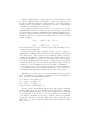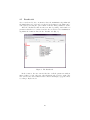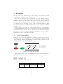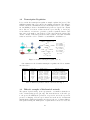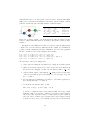
1
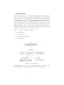
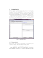
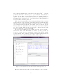
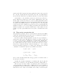
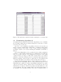
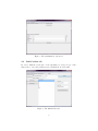
User Manual
Alida Palmisano, Paola Lecca, Corrado Priami
The Microsoft Research - University of Trento
Centre for Computational and Systems Biology
[email protected]
Contents
1 Introduction
2 Getting Started
2.1 The model tab . . . . . . . .
2.2 Time series concentration tab
2.3 Maximization algorithm tab .
2.4 Initial values tab . . . . . . .
2.5 Results tab . . . . . . . . . .
2
.
.
.
.
.
.
.
.
.
.
.
.
.
.
.
.
.
.
.
.
.
.
.
.
.
.
.
.
.
.
.
.
.
.
.
.
.
.
.
.
.
.
.
.
.
.
.
.
.
.
.
.
.
.
.
.
.
.
.
.
.
.
.
.
.
.
.
.
.
.
3
3
5
6
8
10
3 Examples
3.1 Gene Transcription . . . . . . . . . . . . .
3.2 Transcription Regulation . . . . . . . . . .
3.3 Didactic example of biochemical network .
3.4 Lotka-Volterra . . . . . . . . . . . . . . .
.
.
.
.
.
.
.
.
.
.
.
.
.
.
.
.
.
.
.
.
.
.
.
.
.
.
.
.
.
.
.
.
.
.
.
.
.
.
.
.
.
.
.
.
.
.
.
.
.
.
.
.
11
11
12
12
14
.
.
.
.
.
4 Getting Help
.
.
.
.
.
.
.
.
.
.
.
.
.
.
.
.
.
.
.
.
.
.
.
.
.
15
1
1
Introduction
KInfer is a software prototype implementing the parameter estimation method
proposed in [14, 1]. This is a new method for estimating rate coefficients from
noisy observations of concentration levels at discrete time points. The method is
an alternative approach, w.r.t. the traditionally least-squares estimator, based
on a probabilistic, generative model of the variations in reactant concentration.
Our method returns the rate coefficients, the level of noise and an error range
on the estimates of rate constants. Its probabilistic formulation is key to a
principled handling of the noise inherent in biological data, and it allows for a
number of further extensions. For a detailed explanation of the mathematical
formulation of the method, we refer the reader to [14, 1].
The tool consists of four main blocks (Fig. 1):
1. the input interface
2. the model generator
3. the maximization algorithm
4. the output interface
Figure 1: Tool Architecture
In this manual we describe how to install and use KInfer, providing also some
tutorial examples in order to help users learn how to use the software.
2
2
Getting Started
KInfer is a parameter estimation software package written in Java. It requires
the Java 2 Runtime Environment (JRE) version 5 or newer, or an equivalent
JRE. KInfer relies upon the JAMA library, a cooperative product of the MathWorks and the National Institute of Standards and Technology (NIST) [2]: this
library is installed within the KInfer directory when the user install the software.
KInfer is distributed in a jar package, so in order to launch the program it
is enough to double-click on the jar file (to run the project from the command
line type the following command “java -jar KInfer.jar”). The initial application
window should appear like the following:
Figure 2: Initial KInfer window
2.1
The model tab
In the left part of Fig. 2 the user can input the set of chemical reactions
describing the kinetics of the system, with the following syntax:
a A + b B + · · · → a0 A0 + b0 B 0 + · · · : k, α, β, . . . ;
On the left-hand side of the arrow, the reactants (A, B, . . . ) and the reactants stoichiometric coefficients (a, b, . . . ) are indicated (separated by an empty
3
space). On the right-hand side of the arrow the products (A0 , B 0 , . . . ) and the
product stoichiometric coefficients (a0 , b0 , . . . ) are indicated. After the list of
products, the user has to specify the name for the rate constant (k in the example above) associated to the reaction, followed by a comma-separated list of
the partial orders of reaction (α, β, . . . ) for that reaction. The specification of
the reaction must end with a semicolon.
While the user is typing, KInfer is automating translating the list of chemical
reactions into the correspondent rate equations, showing the result in the upper
right part of Fig. 2, with possibly typing errors that prevent the tool to build the
correct mass action model. The list of the partial orders of reaction is optional:
if not specified, the default value can be chosen by the user between 1 (that is
the option “Default ONE”) and the stoichiometric coefficient associated with
the species (that is the option “Default STE”).
To load a model definition file into KInfer, select the “Load reactions...”
item from the “File” menu. This will show a classical open dialog box that can
be used to open the directory containing the textual reaction list file (usually
provided with the “.kin” extension). Opening the Goutsias’ transcription model
explained in section 3, the main window should look like in Fig. 3:
Figure 3: The main window with the Goutsias’ transcription model
The user can save the list of the reactions selecting the “Save reactions...”
4
item from the “File” menu and selecting a path and a name for the new model
file, or he/she can just click the button in the lower left corner (this will save
the model in the current directory, with the name showed on the button label).
As alternative to the automatic generated model, the user is allowed to
insert a different model, that can be entered in the “Manual Model” part of the
interface (Fig. 2). The user is allowed to enter an ordinary differential equation
model without specifying the reaction in the standard chemical notation, and
the syntax of the ODE model has to be the same as the one of the automatic
generated model (some examples are presented in section 3). In particular the
manual model has to be used for specifying general mass action laws with real
numbers as partial order of reaction: in this version of the software, it is not
possible to specify a general kinetic law, but we plan to add this feature in the
future.
2.2
Time series concentration tab
Along with the specification of the set of reactions involved in the system, KInfer
requires the experimental time series data of the concentrations (or number of
molecules) of the species present in the system.
In order to load those data, the user has to select the “Load concentrations...”
item from the “File” menu. This will show a classical open dialog box that can
be used to open the directory containing the concentrations file. This file has to
be a Comma Separated Values (CSV) file, whose first row contains the names of
the columns with the following convention: the first name is the keyword “time”
followed by a comma and the list of all the reactants sp1 , . . . , spN contained
in the model (always separated by a comma). The following rows of the file
contains the concentrations expressed by real numbers as follows:
t0 , [sp1 ]t0 , [sp2 ]t0 , . . . , [spN ]t0
...
ti , [sp1 ]ti , [sp2 ]ti , . . . , [spN ]ti
...
tM , [sp1 ]tM , [sp2 ]tM , . . . , [spN ]tM
where ti is the i-th time instant value and [[spj ]k ] is the concentration value of
the j-th species at time k.
Opening the Goutsias’ transcription concentration file and choosing the
“Time series concentration” tab, the main window should look like in Fig. 4:
The user can see the list of all the concentrations point for all the species
of the system (Fig. 4). In this version of KInfer there is not the possibility of
modifying those data from the interface, but in the next version we plan to add
this feature in order to improve the usability of the loading concentrations part.
5
Figure 4: The main window with the Goutsias’ transcription concentration file
2.3
Maximization algorithm tab
As explained in [14, 1], KInfer uses the Genetic Algorithm in order to maximize
the probability density function calculated using the model and the concentration data provided by the user.
Our choice of the optimization algorithms is driven by the fact that our
method could theoretically handle a high number of parameters with possible
nonlinear relations between them: because of that, traditional optimization
algorithms could have some troubles in finding the maximum of the likelihood
function.
Genetic Algorithms (GA) [3, 4] are population based stochastic optimization
technique, i.e. methods that, starting from a set of initial guesses, determine the
next set of possible solutions to the optimization problem based on the results
obtained from the preceding set. These kind of methods have been designed
primarily to address problems that cannot be tackled through traditional optimization algorithms. Such problems are characterized by discontinuities, lack
of derivative information, noisy function values and disjoint search spaces.
Very briefly, in the GA approach, the evolution starts from a population of
randomly generated individuals. Then in each generation the fitness of every
individual in the population is evaluated and multiple individuals are stochastically selected from the current population (based on their fitness). The chosen
individuals are modified (recombined and possibly randomly mutated) to form
a new population. The new population will be used in the next iteration of
the algorithm. The algorithm terminates when either a maximum number of
6
generations has been produced, or a satisfactory fitness level has been reached
for the population.
The selection operation involves the evaluation of each possible solution with
respect to the target assigned: the higher the log-likelihood value is, the better
the solution is considered. The next step is to select the solutions for the next
generation in such a way that those with higher fitness have higher probability
of selection: to each guessed solution will be assigned a selection probability
derived by the ratio of its square fitness and the sum of the squared fitness of all
the solutions. The selected solutions are then subjected to cross-over, mutation
and innovation operators.
To realize cross-over, every two parents create two children in the following
way: the algorithm selects randomly from the first parent how many and which
variables will have to be kept in the first child. Then from the second parent the
algorithm takes the complementary number of variables and uses these values
to complete the first child. The second child is then built with the remaining
variables of the two parents.
The mutation operation, with a low probability (in our examples p = 0.1),
randomly selects one variable to be mutated. After the selection, the value of
the variable is changed selecting (again randomly) from the possible values it
can take excluding the current one.
Finally, the innovation operator randomly select new solutions never tested
to be performed. Usually this operator is kept at low rate (here at 5%), trying
to optimize the trade-off between exploration and exploitation. Once the new
population of experiments is derived from the algorithm it is then proposed as
a new generation for the next algorithm iteration. The size of each population
of solutions in each generation is maintained constant.
Using the “Maximization options” tab (Fig. 5), the user can modify the
main parameters of the method, in particular:
• Multiplier : a real number, that is used to perform subsequent run of the
algorithm on the same objective function but with different initial value
ranges for the unknown parameter. E.g. using a 0.5 multiplier means that
for each complete run of the GA, the range of the initial parameters search
space is halved.
• NTrial : is the number of different runs of the algorithm that are performed
applying, each time, the Multiplier parameter to the parameters bounds
• NGenerations: is the maximum number of generations of the GA
• Nexp: is the size of each population in a single step of the GA
• Crossed : is the number of population elements that are target of the crossover operation between two steps of the GA. This number has to be lower
than Nexp and it has to be even.
7
Figure 5: The maximization options tab
2.4
Initial values tab
In order to limit the search space of the algorithm, we developed a procedure
that is able to select the parameter space in which the model is valid.
Figure 6: The Initial Values tab
8
Using the “Initial values” tab (Fig. 6) the user can take advantage of this
procedure by simply clicking the “Calculate!” button in the upper part of
the window. This will calculate the Stineman value for each of the parameter
indicated in the model, using the concentrations loaded before, considering that
each value has a measurement error associated.
For a detailed description of the procedure, we refer the reader to [1], but,
summarizing the method, we obtained the slopes in each time point from the
experimental data by using the Stineman algorithm (this algorithm provides a
procedure of interpolation and returns the slope of the interpolating function
running through a set of points in the xy-plane) and we solve the following
system of equation:
si (t1 )
=
...
si (tM )
fi (X(i) ; θi1 , θi2 , . . . , θiNi , σ)
...
=
fi (X(i) ; θi1 , θi2 , . . . , θiNi , σ)
where the functions are the rate equations generated automatically by the set
of reaction or the manual ones.
In general the system could be singular. In those cases, we considered a
different time re-sampling of the Stineman curve interpolating the experimental
data. The new set of time-points are those in which the values of the interpolating curve has null slope. In this way the curve is under-sampled and the
system has a less number of equations. Nevertheless, it may be not enough to
avoid having singular systems. The number of equations is cut down further
on, until the system can be solved to find the approximated values of unknown
parameters to be used as initial guesses for the algorithm of optimization.
In an analogous way, we solve a system of equations for the propagation of
the concentrations error on the estimated parameters in order to find a range
of variability for the single values found by the procedure described above.
This whole process can be avoided by the user that already knows a possible
range of variability for each parameter: in this case the user can simply load
those data from a textual file written as follows:
k1 =>
k2 =>
k3 =>
sigma
lower: 1.0E-8 upper: 1.0
lower: 1.8 upper: 10.0
lower: 0.27 upper: 1.0
=> lower: 1.0E-8 upper: 1.0
The user can also dynamically modify each range value using the graphical
interface (Fig. 6): it is enough to select the parameter that has to be changed in
the central list, and then the user can type the new range in the two textfields
on the right part of the window. To save those values for the current run
of the inference algorithm, the user has to click the “Update ranges initial
parameters!” button. To save them for future runs the user can click the “Save
initial values. . . ” button on the left, and then select a file in which the values
has to be stored.
9
2.5
Results tab
As soon as the model, the concentration data, the maximization algorithm and
the initial values are loaded and correctly set up, the inference algorithm can be
called, just by selecting the option “Infer!” from the “Infer parameters” menu.
After the calculations, that can take some time depending on the number of
parameters that has to be inferred and the choices made for the maximization
algorithm, the results are listed in the “Results” tab (Fig. 7).
Figure 7: The Results tab
In the textarea, the user can find the list of all the parameters with an
inferred value for each of the run of the GA that he/she decided to make. The
user can select the data results from the textarea and simply copy/paste them,
according to his/her needs.
10
3
Examples
Here we provide some validation tests both on simple and complex biochemical
networks. More examples are provided in [1].
For each case study we briefly describe the set of biochemical reactions,
and we report our estimates of the kinetic rate constants compared with the
estimates obtained by other studies and approaches. We did not include in
the text of this tutorial the experimental and/or synthetic time series of the
concentrations we used as input of our procedure to infer the parameter. They
are separately provided as additional files when the user download the KInfer
software tool.
All the results provided here are obtained with a single run of the maximization algorithm with the default values of GA parameters. The variability ranges
of the inferred kinetic rates are the one estimated by the Stineman algorithm,
with an error on the concentration measurements that is chosen according to
the numeric precision of the time series data.
3.1
Gene Transcription
In this test, we consider the transcription of a single gene as given by the model
of Golding et al. in [5]. The DNA for the tagged mRNA is switched on and
off by polymerase binding and unbinding, respectively. Only polymerase-bound
DNA is transcribed into mRNA (Fig. 8).
k1
DNA OFF → DNA ON
k2
DNA ON → DNA OFF
k3
DNA ON → DNA ON + mRNA
k1 = 0.0270 min−1
k2 = 0.1667 min−1
k3 = 0.40 min−1
Figure 8: Gene transcription example
The system is defined by the following list of reactions and our estimates are
summarized in table 1:
DNA_OFF -> DNA_ON : k1;
DNA_ON -> DNA_OFF : k2;
DNA_ON -> DNA_ON + mRNA : k3;
Parameter
k1
k2
k3
σ
Actual value
0.0270
0.1667
0.40
-
Initial guesses
[0.0226 - 0.0302]
[0.155 - 0.163]
[0.374 - 0.425]
[0.03 - 0.45]
Estimated value
0.0248 ± 0.0076
0.163 ± 0.008
0.376 ± 0.052
0.44
Table 1: Estimated parameter values for the network in Fig. 8
11
3.2
Transcription Regulation
Let’s consider the transcription regulation example explained in [12, 13]. The
mRNA is translated into a protein monomer M that can dimerise. The dimer D,
in turn, can bind to its DNA and acts as a transcription factor to auto-regulate
its own mRNA production. Both mRNA and protein are degraded at constant
rates. The set of reactions of this network is reported in Fig. 9. As in [13],
we used this set of reactions to generateto generate a synthetic dataset of the
time series of the number of molecules for each component in the system. The
dataset contains of 120 data point at the time resolution of 0.5 min. As initial
values we used M = 2, D = 4, DNA = 2, and mRNA = 0, DNA·D = 0.
k1
mRNA → mRNA + M
k1 = 0.043s−1
k2 = 0.0007s−1
DNAD → mRNA + DNAD k3 = 0.0715s−1
k4
mRNA →
k4 = 0.00395s−1
k5
k5 = 0.02s−1
DNA + D → DNAD
k6 = 0.4791s−1
k6
DNAD → DNA + D
k7 = 0.083s−1
k7
M+M→D
k8 = 0.5s−1
k2
M→
k3
k8
D→M+M
Figure 9: Goutsias’ transcription regulation [12, 13]
Our estimates for the Goutsias transcription regulation model are summarized in table 2.
Parameter
k1
k2
k3
k4
k5
k6
k7
k8
σ
Actual value
0.043
0.0007
0.0715
0.00395
0.02
0.4791
0.083
0.5
-
Initial guesses
[0.0432 - 0.0432]
[0.015116 - 0.015117]
[0.06931 - 0.06938]
[1.87 - 3.03]E-04
[0.01567 - 0.01568]
[0.3862 - 0.3864]
[0.0838782 - 0.0838783]
[0.515376 - 0.515379]
[0.07 - 0.5]
Estimated value
0.043290182 ± 0
0.015117 ± 0.000000805
0.069322284 ± 0.000069368
0.00021555029 ± 0.0001163084
0.015681929 ± 0.000008789
0.38645026 ± 0.00019106
0.083878241 ± 0.000000073
0.51537892 ± 0.00000304
0.4
Table 2: Estimated parameter values for the network in Fig. 9
3.3
Didactic example of biochemical network
The system depicted in Fig. 10 is representative of a small biochemical network of 4 interacting species ([11, 10]). The network has two feedback loops:
1. the species X3 inhibits the production of species X1 , and 2. the species X4
promotes a changing of X3 in a specie that is not in the model. A numerical
implementation with typical parameters is given by the set of ordinary differential equations in Fig. 10. This system of equations has been used to create the
12
artificial time series of 51 data points, between 0 and 5. Typical units might
mM for the concentration and minutes for the times, but the example could as
well run on an hourly scale and with variables of different nature.
X10 = θ1 X3−0.8 − θ2 X10.5
X20 = θ3 X10.5 − θ4 X20.75
X30 = θ5 X10.75 − θ6 X30.5 X40.2
X40 = θ7 X10.5 − θ8 X40.8
X1 (t0 ) = 1.4
X2 (t0 ) = 2.7
X3 (t0 ) = 1.2
X4 (t0 ) = 0.4
Figure 10: A didactic example of biochemical network with four variables and the
system of ordinary differential equations describing it. The parameter values are listed
in Table 3
The input model for KInfer is not a list of reactions because the kinetics laws
contain order of reaction that are different from the default ones. In KInfer is
possible to input a manual model in the “Manual model” field of the graphical
interface, and the model for this example is the following:
f_x1
f_x2
f_x3
f_x4
=
=
=
=
k1
k3
k5
k7
*
*
*
*
(1)
(1)
(1)
(1)
*
*
*
*
[x3]^(-0.8) + k2 * (-1) * [x1]^(0.5)
[x1]^(0.5) + k4 * (-1) * [x2]^(0.75)
[x2]^(0.75) + k6 * (-1) * [x3]^(0.5) * [x4]^(0.2)
[x1]^(0.5) + k8 * (-1) * [x4]^(0.8)
The user has to follow some simple rules:
1. each row is representing the rate function for a single species in the system
2. all the species in the system need to have an associated rate function (if
the species is not changing over time, the rate function will be “f S = 0”)
3. each rate function has to start with the “f ” string, followed by the name
of the species (without spaces and taking care of lower-upper case) and
the “=” symbol
4. the rate function is a summation of terms (i.e. each term is separated by
the following through a “+” symbol)
5. a term in the rate function has to be like
k6 * (-1) * [x3] ^ (0.5) * [x4] ^ (0.2)
So it has to contain the name of the parameter (k6), followed by a multiplicative symbol (*) and the coefficient (-1) between round brackets,
followed by a list of product terms (i.e. terms separated by the * symbol)
and each of those terms is a species name (x3) between square brackets
elevatated to the power (^) of a real number (0.5) between round brackets
13
In the next version of KInfer we plan to add a more easy way for specifying the
kinetic laws from the graphical interface.
Within the experimental uncertainties, the results showed in 3 are in agreement with the expected ones and with those in [10].
Parameter
θ1
θ2
θ3
θ4
θ5
θ6
θ7
θ8
σ
Actual value
12
10
8
3
3
5
2
6
-
Initial guesses
[11.678 - 11.760]
[9.751 - 9.786]
[6.542 - 6.783]
[2.445 - 2.551]
[3.006 - 3.011]
[4.999 - 5.022]
[1.826 - 1.950]
[5.542 - 5.790]
[0.03 - 0.45]
Estimated value
11.702 ± 0.083
9.765 ± 0.034
6.617 ± 0.241
2.519 ± 0.106
3.011 ± 0.005
5.005 ± 0.024
1.903 ± 0.124
5.588 ± 0.249
0.44
Table 3: Estimated parameter values for the network in Fig. 10
3.4
Lotka-Volterra
The set of coupled, autocatalytic reactions of Lotka-Volterra ([9]) are given
in Fig. 11. The first reaction describes how a certain predator species Y2
reproduces by feeding on a certain prey species Y1 ; the second reaction describes
how Y1 reproduces by feeding on a certain foodstuff, which is assumed to be only
insignificantly depleted thereby; and the third reaction describes the eventual
demise of Y2 through natural causes.
k1
X + Y1 → Y1 + Y1
k2
Y1 + Y2 → Y2 + Y2
k3
Y2 → Z
k1 = 0.0001
k2 = 0.01
k3 = 10
Figure 11: Lotka-Volterra example
We generated a synthetic dataset of time-course of the amounts of X, Y1 , Y2
to use as experimental input data to KInfer with the following values of the rate
coefficients θ1 = 0.0001, θ2 = 0.01, θ3 = 10, and the following initial amounts
Y1 = Y2 = 103 ; X = 105 , and Z = 0. as in [9]. We generated 100 data points
at time steps of about 0.3 and the results that we obtained are listed in 4.
Parameter
k1
k2
k3
σ
Actual value
0.0001
0.01
10
-
Initial guesses
[0.00009739 - 0.0001035]
[0.00689 - 0.00701]
[6.599 - 6.753]
[0.01 - 0.15]
Estimated value
0.0001 ± 0.00001
0.007 ± 0
6.7 ± 0.2
0.1
Table 4: Estimated parameter values for the network in Fig. 11
14
4
Getting Help
If the KInfer program does not function in accordance with the descriptions in
this manual, or if there are sections of this manual that are incorrect or unclear,
the authors would like to hear about it, so that we can make improvements and
fix bugs in the software. Furthermore, the author would appreciate feedback
regarding new features or improvements that would be useful to users of this
software. Before e-mailing the author, it is a good idea to check the KInfer
application home page to see if a new version has been released, in which the
specific problem may have been fixed. The best way to contact the author is to
send e-mail to kinferATcosbi.eu.
When reporting a bug, or something that is suspected to be a bug, please
provide as much information as possible about specific installation of the KInfer program. In particular, please provide us with the version number of the
KInfer program that is used, the type and version number of the Java Runtime
Environment used (e.g., Sun JRE version 1.4.1), and the operating system type
and version. Furthermore, if the problem is with a specific model definition file,
please send us the model definition file, and any model definition files/input
data that it includes. If the problem generated a “stack backtrace” on the console or in a dialog box, please include the full stack backtrace text in the bug
report. Providing this information will dramatically increase the likelihood that
the author will be able to quickly and successfully resolve the problem that has
been encountered.
References
[1] Lecca P. , Palmisano A. , Priami C. , Sanguinetti G., Calibration of
biochemical network models, 2008, Technical Report TR-13-2008, http:
//www.cosbi.eu/Rpty_Tech.php
[2] http://math.nist.gov/javanumerics/jama
[3] Goldberg D. E., Genetic algorithms in search, optimization and machine
learning, 1989, Addison Wesley, Massachusetts
[4] Mitchell M., An introduction to genetic algorithms, 1996, The MIT Press,
Cambridge, MA
[5] Golding I., Paulsson J., Zawilski S. M., Real-time kinetics of gene activity
in individual bacteria, 2005, Cell , 123, 1025-1036
[6] Sugimoto M., Kikuchi S., Tomita M., Reverse engineering of biochemical
equations from time-course data by means of genetic programming, 2005,
BioSystems, 80:155-164
[7] Fuguitt R., Hawkings J. E. Rate of thermal isomeration of α-pinene in the
liquid phase, 1947, JACS , 69, 461
15
[8] Rodrigez-Fernandez M., Mendes P., Banga J., A hybrid approach for efficient and robust parameter estimation in biochemical pathways, 2006,
BioSystems , 83: 248-265
[9] Gillespie, D. T. Exact stochastic simulation of coupled chemical reactions.
J. of Physical Chemistry, 1977, 81 (25).
[10] I-Chun Chou, Harald Martens, Eberhard O Voit Parameter estimation in
biochemical systems models with alternating regression, Theoretical Biology
and Medical Modelling 2006, 3:25, 2006
[11] E. O. Voit and J. S. Almeida Decoupling dynamical system for pathways
identification from metabolic profiles, Bioinformatics 2004, 20, 1670-1681
[12] Goutsias, J. A hidden Markov model for transcriptional regulation in single
cells, IEEE/ACM Trans. Comput. Biol. Bioinform. ,2006, 3, 57-71.
[13] Reinker, S., Altman, R. M., & Timmer, J. Parameter estimation in stochastic biochemical reactions, 2006, 153 (4).
[14] Lecca, P., Sanguinetti, G., Palmisano, A., & Priami, C. A new method for
inferring rate coefficients from experimental time-consecutive measurement
of reactant concentrations. International Conference on Systems Biology,
2007 (ICSB-2007), Long Beach, California, USA.
16