Download Mains Frequency Fluctuation Metering

Mains Frequency Fluctuation Metering
A thesis submitted to the School of Engineering and Information
Technology, Murdoch University in partial fulfilment of the requirements
for the degree of Bachelor of Engineering
By Dusan Sibanic
November 2013
i
I Acknowledgements
I would like to thank Dr. Gareth Lee for his supervision, helpful feedback and
guidance throughout the duration of this thesis.
My deepest thanks go out to my family, partner and friends for their
continuous support. Your patience and understanding through the duration of
this thesis gave me motivation and momentum from beginning to end.
I would like to extend a special thank you to Mark Purvis for his support with
the SD Card shield and relevant libraries, and Michael Chapman for his
generosity with additional components in the project.
Thank you to all the people working alongside me in the E&E building’s project
room and pilot plant. You folks made the long days seem shorter! That’s what
it’s all about, you have to enjoy life.
Acknowledgements go to Arduino and all the hard-working open-source library
developers that allow interesting projects to continue to come to fruition.
For all future thesis students reading this, I wish you luck and encourage you to
persist in your studies.
1
II Abstract
Detecting the frequency of the mains supply is a crucial component of maintaining the grid
frequency at its nominal level. Most frequency counters enable the user to monitor frequencies but
monitoring frequency variations at a high resolution is often expensive. Electronic systems that
measure frequency also have to generate a local time base to calculate the frequency upon. All time
bases suffer from the effect of frequency jitter, which makes the timing source deviate from the
nominal second by a quantified amount. Modern systems have improved drastically and have
relatively insignificant jitter for most timing applications, but high-precision applications require a
quantification of this source of timing error.
The purpose of this thesis is to document the background, implementation, testing, results and
identified future improvements for a frequency meter that can record minor fluctuations of the grid
frequency. By achieving this objective, the grid supply and demand data can be logged and used for
several applications, such as network forecasting or maintaining nominal grid frequency.
An extensive research period was required to determine key design facets pertaining to the
frequency meter. Key identified tasks included choosing a timing source, finding a suitable software
development platform and associated hardware, developing a graphical software implementation
that displays real-time frequency fluctuations, contingency alarming for nominal frequency deviation
events, communications design between the frequency meter and the PC, quantifying clock
precision and evaluating the performance of the final frequency meter.
A GPS time source was chosen to provide an accurate source of 1 second pulses. An Arduino Due
microcontroller used a KX-7 quartz crystal oscillator to maintain its time base and the accuracy of the
KX-7’s time base was analysed against the Trimble Copernicus II and GlobalSat EM406-A GPS
receivers’ time base. When analysed relative to the GPS receivers’ accurate time base, the KX-7
maintained a low time base variation, well within it’s data sheet specifications.
The Arduino Due microcontroller was programmed and provided relevant frequency data to a
LabVIEW PC terminal, which allowed frequency visualisation, data storage, grid frequency
contingency detection, recovery time logging, GPS initialisation data and cross-platform
communication protocols.
Frequency data was logged on the frequency meter and was able to provide a microHertz resolution.
The primary limitation of the design was low-level noise on the mains supply line as this affected the
designed electronics when logging frequency measurements below the milliHertz range. Multiple
recommendations for future work have been identified and included in this report.
2
III Thesis Contents
I Acknowledgements .............................................................................................................................................. 1
II Abstract................................................................................................................................................................ 2
III Thesis Contents................................................................................................................................................... 3
IV List of Figures ...................................................................................................................................................... 5
V List of Tables ........................................................................................................................................................ 6
VI List of Equations ................................................................................................................................................. 7
VII List of Abbreviations .......................................................................................................................................... 8
1 Introduction ......................................................................................................................................................... 9
1.1 Measurement Uncertainty ........................................................................................................................... 9
1.2 Frequency Detection .................................................................................................................................. 10
1.2.1 Measurement Error Sources ............................................................................................................... 10
1.2.2 Counting Method ................................................................................................................................ 12
1.2.3 Frequency Counters ............................................................................................................................ 13
1.2.4 Heterodyning ...................................................................................................................................... 13
1.2.5 Aliasing ................................................................................................................................................ 13
1.2.6 Accuracy of Modern Systems.............................................................................................................. 14
1.3 Thesis Purpose............................................................................................................................................ 14
1.4 Thesis Outline ............................................................................................................................................. 15
2 Background ........................................................................................................................................................ 16
2.1 Timing Methods ......................................................................................................................................... 16
2.1.1 Atomic Clocks ...................................................................................................................................... 16
2.1.2 Radio Clocks ........................................................................................................................................ 17
2.1.3 Crystal Oscillators................................................................................................................................ 18
2.1.4 Time Protocols .................................................................................................................................... 19
2.1.5 Global Positioning System................................................................................................................... 20
2.2 Grid Parameters ......................................................................................................................................... 23
3 Hardware Implementation ................................................................................................................................ 24
3.1 Micro-Controller Unit ................................................................................................................................. 24
3.2 Frequency Detection Shield ....................................................................................................................... 27
3.3 Trimble Copernicus II.................................................................................................................................. 30
3.4 GlobalSat EM406-A .................................................................................................................................... 34
3.5 MAX232 Communications Shield ............................................................................................................... 36
3.6 GPS Jitter Analysis Circuit ........................................................................................................................... 37
4 Software ............................................................................................................................................................ 39
4.1 NI LabVIEW 2013 ........................................................................................................................................ 39
3
4.1.1 Control Panel VI .................................................................................................................................. 40
4.1.2 Supporting Functions .......................................................................................................................... 41
4.2 Arduino ....................................................................................................................................................... 44
4.2.1 PPS ISR Processing Time...................................................................................................................... 44
4.2.2 Alternate Microsecond Function Implementation ............................................................................. 45
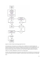
4.2.3 Frequency Metering ............................................................................................................................ 46
5 Timing Precision ................................................................................................................................................. 49
5.1 Arduino Frequency Stability Data............................................................................................................... 49
5.1.1 Clock Drift Relative to Trimble Copernicus II ...................................................................................... 49
5.1.2 Clock Drift Relative to GlobalSat EM406-A ......................................................................................... 53
6 Frequency Meter ............................................................................................................................................... 56
6.1 Setup .......................................................................................................................................................... 56
6.1.1 Hardware Components ....................................................................................................................... 57
6.1.2 Program Parameters ........................................................................................................................... 57
6.2 Performance Results .................................................................................................................................. 60
7 Recommendations and Future Improvements .................................................................................................. 62
8 Conclusion ......................................................................................................................................................... 63
9 References ......................................................................................................................................................... 64
Appendices ........................................................................................................................................................... 68
Appendix A – Arduino Program ........................................................................................................................ 68
Appendix B – LabVIEW Program ...................................................................................................................... 68
Appendix C – Referenced Material .................................................................................................................. 68
Appendix D –Logging Session Data .................................................................................................................. 68
Appendix E – Annotated Bibliography ............................................................................................................. 70
Fundamentals of Quartz Oscillators [9] ....................................................................................................... 70
Relative timing characteristics of the one pulse per second (1PPS) output pulse of three GPS receivers
[51] ............................................................................................................................................................... 70
Accurate measurement of the mains electricity frequency [40] ................................................................. 70
Electronic Navigation Systems [18].............................................................................................................. 70
Trimble Copernicus II GPS Receiver - Reference Manual [45] ..................................................................... 71
Indoor positioning based on global positioning system signals [52] ........................................................... 71
ISO 5725-1 [40] ............................................................................................................................................ 71
4
IV List of Figures
Figure 1. Measurement precision and trueness relative to a referenced standard.
Figure 2. Illustration of jitter on a periodic waveform.
Figure 3. TIE generated by the real-waveforms jitter relative to the ideal waveform.
Figure 4. Gating error magnitude increase due to lower sampled waveform frequency.
Figure 5. Aliased sinusoidal waveform due to an under-sampled signal.
Figure 6. XO circuit model (a) and passive-element equivalent model (b).
Figure 7. GPS Satellite signal transmission path diagram.
Figure 8. Arduino Due MCU.
Figure 9. TI AC-9131 AC-AC step-down conversion adapter.
Figure 10. Stepped-down AC waveform oscilloscope screenshot.
Figure 11. Frequency tracking pulse generation circuit (Eagle schematic).
Figure 12. Oscilloscope output of frequency tracking pulse generator.
Figure 13. Trimble Copernicus II DIP module.
Figure 14. Various elevation mask angles of GPS Satellites referenced to a North Pole positioned
receiver.
Figure 15. EM406-A GPS receiver module.
Figure 16. EM406-A connector cable.
Figure 17. EM406-A cable connection diagram.
Figure 18. Arduino Due / RS232 communication compatibility shield (EAGLE schematic).
Figure 19. GPS relative frequency stability analysis circuit (Eagle Schematic).
Figure 20. Inverted NAND gate voltage output.
Figure 21. GPS receivers’ in-phase (default 1µs and 4µs length) PPS signals.
Figure 22. Control Panel VI user interface.
Figure 23. NMEA Configuration VI user interface.
Figure 24. NMEA checksum generation illustration.
Figure 25. NMEA Packet Decoder VI user interface.
Figure 26. ISR clock-cycle quantifying program.
Figure 27. Previous Arduino library implementation of micros().
Figure 28. New interrupt functioning implementation of micros().
Figure 29. Arduino frequency metering program flow-chart.
Figure 30. Histogram of PPS generated time intervals on the Arduino Due (Copernicus II PPS source).
Figure 31. Arduino 48 hour mean-centered jitter graph (Copernicus II source).
Figure 32. Arduino 48 hour TIE graph (Copernicus II PPS source).
Figure 33. Histogram of PPS generated time intervals on the Arduino Due (EM406-A PPS source).
Figure 34. Arduino 48 hour mean-centered jitter graph (EM406-A PPS source).
Figure 35. Arduino 48 hour TIE graph (EM406-A PPS source).
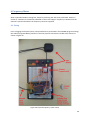
Figure 36. Physical frequency meter setup.
Figure 37. Trimble Copernicus II connected pins diagram.
Figure 38. PPS ISR for timing precision analysis.
Figure 39. PPS ISR for frequency metering.
Figure 40. Statements given in main Arduino loop.
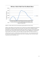
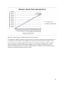
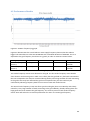
Figure 41. 48 Hour frequency log graph.
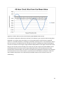
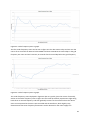
Figure 42. Under-frequency Event 1 graph.
Figure 43. Under-frequency Event 2 graph.
5
V List of Tables
Table 1. GPS system error source table.
Table 2. SWIS grid operational parameters.
Table 3. SWIS target recovery times for grid frequency variations due to contingencies.
Table 4. Arduino Due specifications.
Table 5. Arduino Due pin connections.
Table 6. Pulse generation circuit’s frequency tracking offset with variations in mains supply power
quality.
Table 7. Trimble Copernicus II GPS receiver specifications.
Table 8. Copernicus II project default NMEA packet configuration with checksums.
Table 9. EM-406A GPS receiver specifications.
Table 10. EM406-A project default NMEA packet configuration with checksums.
Table 11. Temperature data for the jitter logging time interval.
Table 12. PPS triggered Arduino 1-second timing interval data (Copernicus II PPS source).
Table 13. PPS triggered Arduino 1-second timing interval data (EM406-A PPS source).
Table 14. Under-frequency events detected during frequency meter performance tests.
6
VI List of Equations
Equation 1. Jitter calculation based on the nominal frequency f and peak frequency variation ∆𝑓.
Equation 2. Determination of frequency using a gating period.
Equation 3. Fractional error of frequency measurement using a gating period.
Equation 4. Calculation of parts-per-million specification based on the center frequency (Hz) and
peak frequency variation (Hz).
7
VII List of Abbreviations
ASCII – American Standard Code for Information Interchange
BIPM – International Bureau of Weights and Measures
BJT – Bipolar Junction Transistor
DMA – Direct Memory Access
ERA – Economic Regulation Authority
GNU – Gnu’s Not Unix
GPS – Global Positioning System
IEEE – Institute of Electrical and Electronics Engineers
IETF – Internet Engineering Task Force
IRQ – Interrupt Request
ISR – Interrupt Service Routine
LCD – Liquid Crystal Display
MCU – Micro-Controller Unit
NMEA – National Marine Electronics Association
NTP – Network Time Protocol
OCXO – Oven-Controlled Crystal Oscillator
PC – Personal Computer
PCB – Printed Circuit Board
PPM – Part(s)-Per-Million
PPS – Pulse-Per-Second output of a GPS
PTP – Precision Time Protocol
RF – Radio Frequency
RMS – Root Mean Square
SV – Space Vehicle
SWIS – South-West Interconnected System
TAI – International Atomic Time
TCXO – Temperature Compensated Crystal Oscillator
TIE – Time Interval Error
TTL – Transistor-Transistor Logic
USB – Universal Serial Bus
UTC – Coordinated Universal Time
VI – Virtual Instrument
WAAS – Wide Area Augmentation System
XO – Crystal Oscillator
8
1 Introduction
1.1 Measurement Uncertainty
This thesis involves analysis of the performance of multiple hardware components. It is necessary to
define the terminology that will be used in the results in order to create a common understanding
between the reader and the author, primarily to avoid misunderstanding and/or vagueness of
terminology. ISO 5725-1 - Accuracy (trueness and precision) of measurement methods [1] is the
international standard used in this study to define the terminology associated with measurements.
All measurements that are made have an associated uncertainty to them. As a general concept, the
uncertainty specifies validity of the result of a measurement [2]. Quantitative measures of
uncertainty may be specified such as variance, standard deviation and range [2].
The precision of measured data relates to how close together the measured values are [1]. Precision
can also be broken down to two components:
•
•
Repeatability – How closely the measurements agree under specified conditions that the
measurement was originally taken under over a short time interval [3].
Reproducibility – How closely the measurements agree with the original set of data under
the same process but different instruments, over a longer time interval [3].
The trueness of a measurement specifies how far the expected measurand is from the reference
value [1]. The data sheets used throughout this thesis will define trueness of a component’s
specification, such as jitter from the nominal operating frequency.
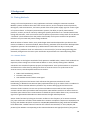
Accuracy is an umbrella term that specifies the overall trueness and precision of measured data. It is
defined as the “closeness of agreement between a test result or measurement result and the true
value” [1]. This is depicted in figure 1.
Figure 1. Measurement precision and trueness relative to a referenced standard [1] [3].
9
Bias is not defined in ISO 5725-1 [3] because it carries a different meaning across different scientific
disciplines. Bias will be defined for the purpose of this thesis as the difference between the expected
measurement and the reference measurement value, which is useful for calibrating instruments [3].
Measurement error is the result of a difference between the obtained measurement and the true
measurement [1] [4]. The measurement error can be broken down into two components, random
error and systematic error. Random error is the unpredictable error detected over a course of
measurements [4]. Systematic error is the quantifiable error that can be predicted over a course of
measurements [4].
1.2 Frequency Detection
Many modern systems rely on frequency detection for standard operation. Quality control of mains
frequency, variable-frequency drives, frequency modulating systems in communications and a
multitude of other electrical systems all use a form of frequency detection to maintain correct
operation. There are many systems available both commercially and for home use to detect the
frequency of various periodic waveforms.
1.2.1 Measurement Error Sources
Frequency measurement can be performed in several ways, depending on the frequency range that
has to be measured and the shape of the waveform. Modern forms of frequency detection include
counting (involving a “gating period”) [5], frequency counters and heterodyning [5] (frequency
conversion). Each method is subject to several issues that affect the accuracy, precision and
measurement error of a measurand. In modern systems, timing source jitter is an issue that creates
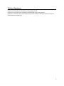
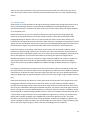
measurement error and contributes to the cumulative time interval error. Jitter (shown as the
interval ‘j’ in figure 2), is the periodic deviation from the nominal period of the source waveform. It is
usually expressed in parts-per-million (PPM), as expressed in equation 1. A ppm specification defines
how many microseconds the signal may be off the nominal value. For example, a 1 part in 20 million
(0.05 ppm) specification will correspond to a ±50ns jitter at a frequency of 1 Hz, whereas a 30 parts
per million jitter specification will correspond to ±30µs from the nominal signal period. Because jitter
is often quantified on the order of micro-seconds or less, this specification becomes useful.
Frequency Source Jitter (𝑝𝑝𝑚) = ±
106 ×∆𝑓
𝑓
(1)
10
Figure 2. Illustration of jitter on a periodic waveform.
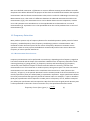
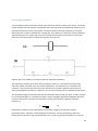
The cumulative time interval error (TIE) is depicted in figure 3. If the cumulative TIE reaches over
±50% of the nominal period, the error will not be recognisable (i.e. a +51% error will be taken as 49%). To ensure the cumulative TIE doesn’t reach this threshold, a clock source with a quantified
jitter should be used and periodically calibrated to a more precise source if required.
Figure 3. TIE generated by the real-waveforms jitter relative to the ideal waveform.
11
1.2.2 Counting Method
Counting is a method for frequency detection and involves recording the number of waveform
periods during a set “gating period”, which is simply a chosen constant time interval [5]. By counting
the number of input signal cycles over a gating period, it is possible to determine the frequency by
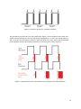
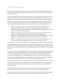
dividing the number of counted cycles over the gating period, as shown in equation 2. The fractional
error associated with this is given in equation 3 and is inversely proportional to the sampled
waveforms frequency, as shown in figure 4.
𝑓=
𝐶𝑦𝑐𝑙𝑒𝑠 𝐶𝑜𝑢𝑛𝑡𝑒𝑑
𝐺𝑎𝑡𝑖𝑛𝑔 𝑃𝑒𝑟𝑖𝑜𝑑 (𝑠𝑒𝑐)
∆𝑓
𝑓
=
1
2∙𝑓∙𝑇𝑚
(2)
(𝐻𝑧)
(3)
Figure 4. Gating error magnitude increase due to lower sampled waveform frequency.
12
1.2.3 Frequency Counters
High frequencies can be measured through frequency counters and several modern technologies
allow this, such as data acquisition cards and microcontrollers. Most frequency counters derive their
time-base from a crystal oscillator (XO) which oscillates at a known frequency [5]. The measured
input frequency is then ascertained by counting the number of periods in a time period generated by
local frequency counter’s XO. The frequency counter method is generally very precise in the shortterm but long-term measurements will be affected by the jitter of the instrument’s time-base
source. Modern frequency counters can currently cover up to a range of 100GHz [5] but are typically
expensive for high-range frequency measurements.
1.2.4 Heterodyning
Heterodyning is the process of mixing two different frequencies to produce a frequency that can be
used in signal processing [6]. The output frequency that is produced is called the heterodyne.
Historically, heterodyning was used to process high frequency signals by mixing them into a
heterodyne that could be processed by the technology that was available. Heterodyning is still used
in RF applications [6], but as frequency counter technology keeps improving to provide higher
sampling rates and costs go down, heterodyning is more suited to fill very high frequency detection
applications.
1.2.5 Aliasing
No matter which method is chosen to detect the frequency, the sampling period must be considered
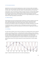
carefully to avoid aliasing. Aliasing is an undesirable effect caused by sampling a periodic waveform
below the Nyquist sampling rate [7]. The Nyquist theorem states that the sampling frequency should
be at least twice the sampled signals frequency [8]. By sampling at less than twice the input
frequency, a false frequency may be sampled. In practical applications, this value should be 5-10
times higher than the sampled frequency as a minimum so that the reconstructed signal is more
defined and less prone to noise. Figure 5 illustrates an aliased sinusoid due to an under-sampled
signal.
Figure 5. Aliased sinusoidal waveform due to an under-sampled signal [5].
13
1.2.6 Accuracy of Modern Systems
Many electronic systems rely on a XO which has a known internal oscillation frequency to provide a
continuous time-base. XOs are relatively cheap and effective but are subject to frequency stability
variations, especially in long-term use and environments with significant temperature variation [9].
The electronics that rely on XOs for a stable time-base are usually precise in the short term. Long
term stability may be significantly affected depending on the crystal’s cut, temperature and material
[9].
To compensate for the frequency instability in electronics that rely on XOs, a more precise timing
signal could be used to either steer the electronic clock to the more precise time source or simply
quantify the error associated with the XO and compensate for this error respectively.
1.3 Thesis Purpose
This project envisages building a precise metering device to monitor small mains supply frequency
fluctuations (on the order of mHz or better). While power utility companies internationally choose to
keep the mains supply frequency at either 50Hz or 60Hz, they have no control over the time at which
customers may connect or disconnect loads. As loads are connected and disconnected from the grid,
the generators that provide power to the grid are adjusted to either slow down or speed up to
maintain the nominal grid frequency. There is a delay involved in the generator’s corrective response
actions and this delay period gives way to typically minor frequency fluctuations on the mains
supply.
A frequency meter has been designed that has a quantified timing precision. The developed meter is
based upon an open-source electronics prototyping board, the Arduino Due [10]. Appropriate
electronics have been developed that connect to this MCU and various methods of keeping an
accurate time-base have been considered such as GPS [11] [12], NTP and PTP [13] [14], atomic clocks
[15], radio clocks [16] and crystal oscillators [9]. The frequency metering unit is able to store grid
frequency data in real-time and transmit this data to a computer for analysis of the supply and
demand ratio on the grid. This high-precision meter has applications in the analysis of load
management, network forecasting, generator response to load variation and contingency analysis.
14
1.4 Thesis Outline
In addition to the abstract, introduction, background and conclusion, the thesis has five key
chapters:
•
Hardware Implementation – This section discusses the hardware chosen for the project, the
specifications that are relevant to each component, how it will contribute to reaching the
project’s goals and how the hardware is connected for various analysis purposes.
•
Software – The libraries used in the software implementation, their purpose in the project
and any additional libraries developed are discussed in this section to detail the approach
taken to meet the project’s goals. The two primary programming languages used are G
(LabVIEW’s graphical programming language) and the Arduino programming language (a
Wiring language derivative).
•
Timing Precision – One of the primary goals of the project was to quantify the precision of
the frequency meter. This is done in this section by analysing the relative clock drift data
between several implementations such as the Arduino Due’s XO, the Trimble Copernicus II
GPS receiver and the EM406-A GPS receiver.
•
Frequency Meter – The frequency metering system is described in the final chapter in the
main body including its overall performance and limitations.
•
Recommendations and Future Improvements – This chapter ties into the conclusion chapter
heavily as the recommendations are drawn from the concluded findings. It outlines future
improvements that may not have been able to be implemented in this project due to various
factors but would be viable in further studies.
15
2 Background
2.1 Timing Methods
Timing is of crucial importance in many applications and time tracking has numerous methods.
Modern systems can derive their time from various sources, such as computer network protocols,
GPS signals, radio transmissions, the known period of the mains power supply signal or various types
of crystal oscillators. In frequency measurement systems, the ability to specify measurement
precision, accuracy and error comes by relating the systems performance to a standard with known
timing characteristics, such as an atomic clock. No perfect system exists to keep track of time but the
“clock drift” (clock deviation from the perfect time model) of all systems is able to be quantified
relative to very accurate and precise timing standards.
With the advent of atomic clocks, many technologies have been developed that synchronise their
timers to rubidium or caesium standards. More recently, ytterbium clocks have been developed that
outperform previous clock standards [17]. While caesium clocks take five days to reach peak
performance, ytterbium clocks can achieve this in one second [17]. Precise timing technology has
drastically changed over the recent years and further improvements are continually being made.
2.1.1 Atomic Clocks
Atomic clocks are the highest standard of clock precision available today. Atomic clock standards are
expensive, often costing tens of thousands of dollars or more, thereby making them a difficult
standard to use outside of expensive projects and experiments. Time synchronisation on computers
and electronics is often done by polling time from an accurate source. To synchronise to this
accurate source, several implementations exist such as:
•
•
•
Radio clock broadcasting stations;
Stratum 1 NTP servers;
GPS Satellites that broadcast a PPS signal.
Radio clocks [16] have a local atomic clock reference that generates time data for radio
broadcasting. In Network Time Protocol (NTP) implementations [14], an atomic clock is considered a
“stratum 0” device. Stratum 0 devices provide a very accurate timing signal and are used as
reference clocks. Stratum 1 servers are synchronised within microseconds to their respective
stratum 0 device and may broadcast NTP time packets. GPS satellites each have an atomic clock onboard the space vehicle. The instrumentation on-board the space vehicle allows a very accurate PPS
signal to be generated and broadcast to GPS receivers through radio frequencies.
Atomic clocks function by locking an electronic oscillator to the frequency of an atomic transition
[15]. Two well-known and often used standards are caesium-133 (which transitions at 9,192,631,770
Hz [15]) and rubidium-87 (which transitions at 6,834,682,610.904324 Hz [18]). Both NIST and BIPM
have defined the “standard second” based on the caesium-133 standard, as “the 9,192,631,770
periods of the radiation corresponding to the transition between two hyperfine levels of the ground
16
state of the caesium 133 atom” [19]. This means that atomic clocks can achieve accuracy on the
order of parts-per-billion, which translates to better performance than any other available timing
source.
2.1.2 Radio Clocks
Radio clocks are synchronised by the RF signal containing time data that timing signal stations send.
The list of broadcasting stations is maintained by the BIPM [19]. The broadcasting stations are
spread internationally. A limitation of radio clocks is that many locations have poor signal reception
or no reception at all.
Radio clock stations all vary in the frequency bands they may output their timing signals [20].
Antennas vary proportionally in size to their output frequency, which affects the length of the
propagated RF signal. Stations also vary in their transmission times, where some stations may
transmit the time signal continuously and others have downtime. The length of the pulse-per-second
signals can also vary between stations [20]. The lack of a standardised timing signal format and time
interval between signals may potentially make radio clocks unsuitable for some applications.
Radio clock stations are primarily connected to atomic clocks such as caesium standards, which
provide an excellent timing reference [16]. The main issue that arises with time synchronisation at
the receiving end is radio signal transfer. Due to the nature of RF wave propagation, significant jitter,
delays and signal loss may be encountered when transmitting the signal over long distances.
Broadcasting stations transmit at a frequency range of 25kHz to 25MHz [21], with the exception of
radio station STFS, which transmits at approximately 2.6GHz [21]. Between 25kHz and 25MHz,
signals fall into the Low (3-30kHz), Medium (0.3-3MHz) and High (3-30MHz) frequency categories
[22].
Low frequency transmissions primarily travel over surface waves, which travel slightly further than
the visible horizon [22]. Past the radio horizon, the signals may reflect off the sky. Medium frequency
transmissions are primarily surface waves during the day with some sky wave reflection during the
night [22]. High frequency signals propagate as sky waves over long ranges using ionospheric returns
[22].
Radio clock technology was chosen to not be relied upon for the purpose of this project due to the
propagation distance from the nearest radio clock station to Perth, Western Australia. While in
principle this technology can be used to synchronise clocks with an accurate reference, the location
this study was conducted at had highly unreliable reception. The nearest radio time signal station to
Perth is call sign JJY, located at Mount Otadakoya, Fukushima, Japan at a distance of 5033km. Under
the assumption of reception being available in Perth, a latency of 16.78ms would be observed due to
a transit delay of approximately 1ms for every 300km the signal has to traverse [16]. Surface wave
signals paths typically propagate up to 1500km [23]. At distances greater than this, the signal
becomes a sky wave signal and refracts off the ionosphere. At distances of 5000km or greater, the
signal’s reliability becomes extremely poor and unusable due to the signal’s irregular pathways [23].
Due to the lack of signal integrity in Perth, alternate technologies were considered.
17
2.1.3 Crystal Oscillators
Crystal oscillators (XOs) have been used in many electronic devices to keep track of time. The quartz
crystal oscillator has the property of piezoelectricity, which provides a link between electronics and
mechanical distortion of the crystal lattice. The XO has stiffness and some elasticity in its bonds,
which allow the crystal to resonate like a tuning fork. The frequency at which the crystal oscillates is
determined by the size, shape and cut of the crystal and the frequency drift that the crystal may
experience with temperature is determined by the size of the cut.
Figure 6. XO circuit model (a) and passive-element equivalent model (b).
The equivalent model in Figure 6 has four parameters, where C1 is the capacitance due to the
electrode, holder and leads, C2 is the notional capacitance, the inductance L1 is related to the
oscillator’s mass and the resistance R1 is due to bulk losses. The XO is typically inserted into an
electronic feedback loop where it oscillates at it’s resonant frequency and is amplified at the output.
The XO model in figure 6 demonstrates that the XO behaves like a band-pass filter, so when coupled
to an external amplifier, it is possible to create a system with gain and positive feedback. Because
C2 and L1 behave like a second order electronic system, they will have a defined resonance
frequency fo:
𝑓𝑜 =
1
2𝜋√𝐿1∙𝐶2
(4)
XO frequency stability can be reduced due to the effects of aging, varying power quality,
gravitational force, vibrations, electromagnetic interference, retrace (essentially a cold start),
temperature and pressure [9]. The temperature of a crystal is of greatest importance as it has the
18
greatest effect on oscillator stability [9]. Three commonly used variations of XOs are affected by
temperature in different lengths. The room temperature XO (RTXO) has no method of temperature
compensation, the temperature compensated XO (TCXO) is cut in a way to minimise changes to its
frequency stability due to temperature changes and is encased to minimise abrupt ambient
temperature changes. The oven controlled XO (OCXO) has the most precise method of oscillatory
frequency stability control [9]. OCXOs control the temperature variation the crystal is exposed to
through a feedback temperature control system, which allows the crystal to perform with
significantly less variation in operating frequency. Most consumer electronics utilise RTXOs due to
their very low cost and ability to keep a timing accuracy within the order of parts-per-million. [24]
2.1.4 Time Protocols
NTP and PTP are protocols designed to synchronise computers over a general purpose computer
network to a high-precision clock standard. Both protocols use a server-client architecture to
transmit UTC time over packet-switched networks. As with any networking protocol, packet errors,
throughput size, latency variation and packet loss can cause the performance of the system to drop
[25]. Applications that require reliable, precise timing will be affected by this performance drop.
NTP is the most common time synchronisation standard in computers today. The IETF maintains
NTPv3, the most common implementation of NTP. RFC 1305 [13] provides the specification,
implementation and analysis of NTPv3. The newest implementation of NTP is NTPv4 [14]. NTP has
several topologies including server-client (where the client periodically polls the server for the time
and calculates its own clock offset), symmetric active-passive mode (NTP data is polled via peers on
the network), broadcast/multicast mode (a server sending NTP packets periodically to a group of
clients or the entire networks) and manycast mode (a client polls several NTP servers to determine
the server with least latency to connect to, then establishes a connection) [26].
PTP is a more recent timing protocol implementation, designed to provide a higher standard of
precision than NTP. PTP is specified under IEEE1588-2008. PTP is primarily intended to provide a
time-base more accurate than NTP in areas where GPS signals are either inaccessible or too costly.
PTP works on a similar principle to NTP but has additional protocol provisions for estimating
propagation and synchronisation delay between the server and the client. Hardware provisions
however must be made to provide this and can be costly for simple applications.
Both protocols are susceptible to the same transmission related delays like any other networking
protocol. Latency is the measure of transmitted signal’s delay and is typically quantified using
algorithms that compute the delay [25]. The number of hops is a significant contributor to the effect
of latency as it reduces end-to-end synchronisation performance [27]. The data rate limit is another
factor that may limit the transmission of the NTP packet, but in most modern networks is not an
issue. Line coding delay [25] comes from both the client and server and is the time that the sender
and receiver take to compute and assemble an outgoing packet as well as the time taken to decode,
generate checksums and error check an incoming packet. Precision on the order parts-per-million is
typical of NTP but the jitter may vary on the order of tens of thousands of ppm.
19
2.1.5 Global Positioning System
The Global Positioning Network had its inception in 1973 to replace the Navy Navigation Satellite
Systems [22]. The GPS satellite network was operational on 27 April 1995 with 24 satellites orbiting
the globe twice a day.
RF waves propagate at the speed of light (299 793 077 ms-1). The GPS signals are sent from space at
a height of 20 200 km, but this distance varies as the satellites follow an elliptical path [22]. GPS
satellites have an orbital period of 11 hours and 58 minutes [22]. Each GPS SV is equipped with four
atomic clocks – two rubidium and two caesium [22]. The initial generation of GPS SVs was Block II,
with the first satellite launched into orbit in February 1989 and final on October 1990. Since then,
several other satellites were launched to provide improvements to the existing infrastructure:
•
•
•
•
Block IIA – 13 satellites of this series still orbit the Earth with the final satellite being
launched on November 1997. This block was designed to allow a longer period of
independent operation with control segment contact (180 days) [28]. Satellites in this block
only operated on the L1 frequency [29].
Block IIR – 12 satellites from this series were launched since July 1997 as “replenishment”
satellites, to replace older satellites that were about to fail or already failed.
Block IIR-M – 8 satellites were launched in this series, with the final being launched in August
2009. These satellites included the L2C signal for more robust civilian use [30].
Block IIF – 12 satellites are due to launch in this series with the second being sent in July
2011. IIF has all of IIR-M’s capabilities introduces a 3rd Civilian Signal (L5). [29]
In May 2012, the contract for the next generation of satellites has been awarded to Lockheed Martin
to provide Block IIIA satellites [29]. The primary benefits of the new generation are higher accuracy,
improved anti-jamming, increased lifetime and backward compatibility with older systems [30]. The
first satellite in this generation is due to launch in 2014 [29] and will also introduce 4th civilian signal,
L1C [30].
In the past, civilian use of GPS suffered from “selective availability”, which was discontinued on May
2, 2000 [31]. Selective availability affected all non-military GPS receivers by increasing the location
error up to 100m away from the true position. This error was unacceptable for high precision
location and timing applications. In timing applications that rely on a GPS receiver’s PPS, this error
caused significant additional timing jitter. A 100m location error generated by selective availability is
equivalent to ±333.6 nanoseconds PPS jitter. Fortunately, this is no longer an issue.
GPS satellites typically transmit at two frequencies- the L1 frequency band (1575.42 MHz) and the L2
frequency band (1227.6 MHz). These frequencies are in the ultra-high frequency band (300-3000
MHz). Radio waves in this frequency band primarily propagate as space waves, which require a
direct line of sight.
GPS broadcasts a Pulse-Per-Second signal to GPS receivers. This signal is generated by an atomic
clock on-board each GPS satellite and is subject to transmission jitter and processing jitter.
Transmission jitter comes from several sources, the largest being from the space wave propagating
through space and Earth’s atmosphere. As an RF wave passes through the troposphere and
20
ionosphere, its speed is reduced. At a height of 80-400km, the RF waves pass through the
ionosphere, which refracts the GPS satellites signals [32]. Because the velocity variations through the
ionosphere are known at GPS transmission frequencies, GPS receivers mostly correct the error
associated with ionospheric delays [32]. Tropospheric delays are caused by refraction and a further
change in the propagation medium. WAAS enabled receivers may receive atmospheric condition
data over different regions which allows the receiver to operate at a much greater accuracy in its
atmospheric delay calculations [32].
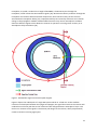
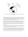
Figure 7. GPS Satellite signal transmission path diagram.
Figure 7 depicts the orbital path of a single GPS space-vehicle on a fixed axis. As the satellites
traverses its orbital path between the apogee and perigee, the signal that travels to the receiver will
undertake a non-linear path due to the refractive index changes between atmospheric layers. This
results in a variation of the signal’s transmission path length to the receiver, which proportionally
creates a variation in timing signal jitter.
21
Error Source
Error Variance
Ionospheric effects
± 5 meters
Satellite orbital shifts
± 2.5 meters
Satellite clock errors
± 2 meters
Multipath effects
± 1 meter
Tropospheric effects
± 0.5 meters
Calculation and rounding error
± 1 meter
Table 1. GPS system error source table [32].
Table 1 explains the variation in GPS signal error due to multiple sources. Variations in the
ionosphere and orbital altitude of the GPS space vehicle account for the largest component of the
GPS error. Modern GPS receivers, especially those with WAAS enabled correction, can account for
most of these errors to improve the accuracy of the received signal data.
These GPS error sources contribute to ± 15 meters of dilution of precision. In WAAS corrected GPS
receivers, if a WAAS correction is able to be obtained, this error goes down to ± 3-5 meters [32]. This
enables GPS receivers to have PPS accuracy on the order of parts-per-billion [33].
22
2.2 Grid Parameters
It is important to know the frequency of the grid as all electronic equipment that is connected to it
has a certain operating frequency requirement. The frequency may dictate the electronics efficiency,
operating limits or it may provide an alternate use, such as providing a time-base in digital timers.
While generally the mains frequency is not used to provide a time-base due to the low cost and high
availability of XOs, it’s nonetheless important for many applications. To measure the frequency of
the grid, the parameters of the grid must be known. In order to design a metering system that will
not damage itself due to fluctuations in the grid, information was taken from Western Power’s
website and the SAIGlobal Standard Voltages document [34]. Western Power is the power utility
company operating in the SWIS region of Western Australia. While Standards Australia defines the
nominal voltage and frequency values for all of Australia [34] in AS60038, Western Power specifies
it’s own operating standards in the Technical Rules document [35].
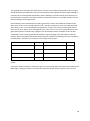
Tolerance Nominal Value Min (%) Max (%)
Voltage
240V RMS
-10
+6
Frequency 50 Hz
Frequency 50 Hz
Table 2. SWIS grid operational parameters. [35]
Min
226 V
49.8 Hz
49.5 Hz
Max
254.4 V
50.2 Hz
50.5 Hz
Mode
SWIS
Islanded
Table 2 shows the operating frequencies for standard and islanded grid connections and the
operating limits for the grid voltage.
The accumulated synchronous time error is defined as “the difference between Western Australian
Standard Time and the time measured by integrating the instantaneous operating frequency of the
power system” [35]. In the SWIS region, this value must be less than 10 seconds for 99% of the time.
Event
Single Contingency
Frequency Band (Hz) Target Recovery Time
48.75 – 51.00
Normal range: <15 mins
Over-frequency events:
<50.5Hz within 2 mins
Multiple Contingencies 47.00 – 52.00
Normal range: <15 mins
Under-frequency events:
1. Above 47.5Hz within 10 secs
2. Above 48.0Hz within 5 mins
3. Above 48.5Hz within 15 mins
Over-frequency events:
1. Below 51.5Hz within 1 min
2. Below 51.0Hz within 2 mins
3. Below 50.5Hz within 5 mins
Table 3. SWIS target recovery times for grid frequency variations due to contingencies. [35]
The parameters in table 3 are primarily used to compare contingencies detected on the frequency
meter against the specified standard to assure the recovery times are within the specified range.
23
3 Hardware Implementation
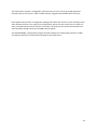
3.1 Micro-Controller Unit
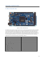
Figure 8. Arduino Due MCU [10].
The Arduino Due [10] (seen in Figure 8) was chosen as the prototyping Microcontroller Unit (MCU)
for the project amongst other MCUs due to its hardware specifications, cost, large collection of
open-source libraries, instant availability and its ability to meet the requirements of the project.
Murdoch University’s Engineering & Information Technology department provided an Arduino Due
for prototyping the metering unit. The Arduino website and Atmel datasheet list the following
specifications for the Arduino Due [10], summarised in table 4.
CPU
CPU Clock
Static RAM
Core Resolution
Flash Memory
DMA Availability
Operating Voltage Range
Digital I/O Pins
Analog Input Pins
Analog Output Pins
Analog Input Range
Analog Output Range
Analog I/O Resolution
Sampling Rate
Table 4. Arduino Due specifications [36] [10].
Atmel AT91 SAM3X8E
84 MHz
96 kB
32 bit
512 kB
Yes
7-12V
54
12
2
0 – 3.3V
0 – 3.3V
10-12 bit (1028 – 4096 values)
1 MS/s
24
Most MCUs available on the market are either 8 bit or 16 bit, typically produced by Arduino [37],
Freescale [38] or Microchip [39]. A Motorola 68HC11/68HC12 [40] was also considered for the
project. Due to the simplicity, availability of support and extensive libraries available on the Arduino
platform, the Arduino Due was a more suitable development platform. The Arduino Due is a lowcost MCU which can perform 32-bit operations at a clock rate of 84 MHz. No other MCU with these
specifications or better could be found at a reasonable cost. These specifications outperformed most
competitors on the market and greatly outperformed all considered competition for its cost.
The Arduino Due is an open source electronics prototyping platform released under the Creative
Commons Attribution Share-Alike license and its public libraries fall under the GNU Lesser General
Public License [41] [42] [43]. Under the share-alike license, all work created upon the Arduino
platform must be distributed under the same license.
In a conference paper by Ibrahim [44], a method for metering the mains frequency is proposed that
utilises a near-zero detector, PIC18F4520 MCU and PC link to acquire periodic pulses, compute the
period between them and log the mains frequency. The design utilised an 8MHz XO on-board the PIC
MCU. This design was considered in the planning stage for the mains frequency meter in order to
choose the hardware components that will meet the project’s goals. It is unclear whether the XO onboard the PIC MCU is temperature compensated in any form. Given that most RTXOs are mounted
onto the MCUs PCB, it was assumed to be an RTXO. This is not an issue in short-term frequency
measurements but does pose an issue long-term. Clock stability is able to be quantified by
examining the on-board MCU drift relative to a more precise timing source, such as GPS PPS or an
atomic standard.
The Arduino Due EAGLE [45] schematic file specifies the on-board 12MHz XO as a KX-7 quartz crystal
with a ±30ppm frequency tolerance at 25°C [24]. The aging specification is rated at ±2ppm/year [24],
but the manufacturing date of the KX-7 crystal was not able to be ascertained. Given that the
Arduino Due is less than 2 years old however, an upper limit was set, giving at most 4ppm additional
jitter.
25
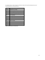
The Arduino Due pins were assigned as outlined in table 5 for all performed experiments and
standard frequency metering operation.
Pin
Description
D0 (RX0) LabVIEW TX (via USB)
D1 (TX0)
LabVIEW RX (via USB)
D7
GPS PPS Signal
D9
Mains Pulses (Frequency Measurement)
D10
SD card (Power)
D11
SD card (MOSI)
D12
SD card (MISO)
D13
SD card (SCK)
D14 (TX3) EM406A RX
D15 (RX3) EM406A TX
D16 (TX2) MAX232 Shield
D17 (RX2) MAX232 Shield
D18 (TX1) COPERNICUS 2
D19 (RX1) COPERNICUS 2
SPI
See Pins D11, D12, D13
Table 5. Arduino Due pin connections.
26
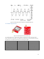
3.2 Frequency Detection Shield
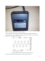
Figure 9. TI AC-9131 AC-AC step-down conversion adapter.
A TI AC-9131 adapter, seen in Figure 9, was utilised to step-down the voltage from the mains
supply’s 240V AC to 3.3V AC. A datasheet was not available for the component. The product label
stated a 240V-3.3V AC-AC step-down conversion.
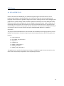
Figure 10. Stepped-down AC waveform oscilloscope screenshot.
Figure 10 displays the observed stepped down no-load voltage of the adapter.
27
The stepped-down waveform was observed at 7.64 VRMS. This waveform appeared to be at the grid
standard frequency of 50Hz [34]. The Johnson noise due to the impedance of the output windings is
unknown due to no datasheet specification and no shielding is provided, hence the noise that may
be potentially introduced to the 50Hz waveform is unknown, and this is a possible source of error in
the final design’s metering precision.
Several designs were considered for the pulse generation circuitry that would be attached to the
MCU input, such as zero-crossing detectors [44], a window-comparator circuit and a BJT [46] pulse
generation circuit. A zero-crossing detector generates a pulse every time a periodic signal crosses
the zero-volt mark. Many “zero-crossing detectors” were in fact “near-zero crossing detectors” that
generated a pulse at a similar input voltage to the developed transistor amplifier circuit. Several
considered circuits involving operational amplifiers required voltages that the Arduino could not
provide. When analysed for the benefit the operational amplifiers would bring over their complexity
and limitations, they were not necessary in the design of this project.
Variation from Nominal Voltage Offset (µs) Variation from Nominal Voltage Offset (µs)
+1%
3.21
-1%
3.28
+2%
6.36
-2%
6.62
+5%
15.46
-5%
17.08
+10%
29.51
-10%
36.07
Table 6. Pulse generation circuit’s frequency tracking offset with variations in mains supply power
quality.
The power quality variations in table 6 are given as a percentage offset from the nominal 240V in the
SWIS region. The given offsets are valid for the respective power quality variation over 1 second.
28
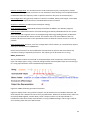
Figure 11. Frequency tracking pulse generation circuit (Eagle schematic).
The frequency tracking circuit is designed to periodically generate digital pulses that are at the same
frequency as the incoming 50Hz sinusoidal waveform. A low-pass filter attenuates the incoming
signal’s frequency past the cut-off point of 500Hz in order to reduce high frequency noise while
minimising attenuation at the 50Hz frequency. A 1N4148 diode is connected with the anode to
ground and the cathode connected to the T1 transistor’s base. This diode allows current to flow
through the capacitor C1 and resistor R4 during the negative cycle of the input waveform. The
diode’s action prevents damage to Transistor T1 as the Emitter-Base voltage cannot exceed more
than 6V [46]. T1 switches on when the base-emitter voltage is above 0.7V [46]. Due to the positive,
non-zero voltage that the transistor turns on at, the square wave that is produced has a mark/space
ratio that is slightly less than 50%, but still easily long enough (on the order of milliseconds) to be
measured by the Arduino, which can measure on the order of microseconds [36]. Figure 12 displays
the transistor’s pulse triggering but it appears that the square wave’s positive and negative edges is
very close to zero due to the larger AC signal voltage.
29
Figure 12. Oscilloscope output of frequency tracking pulse generator.
3.3 Trimble Copernicus II
Figure 13. Trimble Copernicus II DIP module [12].
The Trimble Copernicus II is a GPS receiver module. The Copernicus II used in this project came
factory mounted to a DIP module. A 3V magnetic-mount SMA antenna was purchased to connect to
the Copernicus II. The SMA antenna boosts the receivers gain by 26dB.
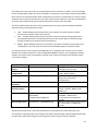
Specification
Value
PPS Accuracy
±60 ns RMS
“
±350 ns RMS
Warm Start Time
35 secs
Cold Start
38 secs
Hot Start
3 secs
Tracking Sensitivity
-160 dBm
Acquisition Sensitivity
-142 dBm
“
-148 dBm
Table 7. Trimble Copernicus II GPS receiver specifications. [33]
Mode
Static
Stationary Mode
No Battery Backup
Standard
High Sensitivity
30
The Copernicus II was chosen due to its specifications which are shown in table 7. The cost and high
level of configurability made the receiver suitable for this project. Several other Arduino shield based
GPS receivers were considered but either lacked features, precision, specifications or were not easily
adaptable for use with the Arduino Due. An older revision of the Copernicus was also considered due
to the price but lacked the precision and functionality the Copernicus II provided.
The stock module allows TTL-level serial communications on 6 ports (3xTX and 3xRX) and allows
communicating in three different formats:
•
•
•
TSIP – Trimble Standard Interface Protocol, this interface is Trimble’s primary packet
transmission standard in their GPS receivers.
TAIP – Trimble ASCII Interface Protocol, primarily suited to vehicle tracking applications.
Considerably powerful in networked environments due to the ability of communicating
through a unique ID in packet based communication.
NMEA – National Marine Electronics Association, this packet standard is supported by the
TinyGPS library and can easily be parsed to the LabVIEW program for packet analysis.
The chosen protocol for this project was NMEA due to its simplicity and to favour a set standard
between the Trimble Copernicus II and the GlobalSat EM406-A modules. The configured messages
used by the receiver can be seen below in table 8. Some of these messages are fixed while others
vary as time changes.
Packet
Automatic Message
Output
Receiver
Configuration
PPS Configuration
Sentence
$PTNLSNM,0021,01*54
Acquisition
Sensitivity
Serial
Communications
$PTNLSFS,S,0*23
$PTNLSCR,,15,,,,0,1,,1*5C
$PTNLSPS,2,5000000,1,0000010*51
Description
Configures receiver to output GGA
messages every second.
15° elevation mask, Stationary
mode, WAAS enabled
Fix-Based PPS, 500ms pulse, Active
HIGH, 10ns cable delay
compensation
Standard sensitivity mode
$PTNLSPT,019200,8,N,1,4,4*1C
19200 Baud, 8 data bits, No parity
check, 1 Stop bit, NMEA in and
NMEA out
Initial Position
$PTNLSKG,GPSW,GPSWMS,
GPSW = GPS Week since first epoch
3203.96635,
GPSWMS = Milliseconds
accumulated since 00:00 UTC
S,11550.22761,E,00010*FF
Sunday
Reset Configuration $PTNLSRT,H,2,2,0000000000*1B
Hot Start, Store User-Config to Flash
on reset, Wake on NMEA port
activity
Table 8. Copernicus II project default NMEA packet configuration with checksums. Implementation
appropriate carriage return and line-feed delimiters should follow all packet checksums [33].
The automatic message output was configured to display GGA messages. GGA messages display GPS
Fix data which allows PPS integrity monitoring based on the number of active satellites.
31
Figure 14. Various elevation mask angles of GPS Satellites referenced to a North Pole positioned
receiver.
The receiver’s configuration had the elevation mask set at 15°. The elevation mask is the minimum
elevation angle between the horizon and the satellite, relative to the receiver (as shown in Figure
14). At 10° elevations and higher, ionospheric and tropospheric signal corruption is reduced as the
atmospheric effects begin to become more predictable for the receiver. The possible limitation of
this approach is exclusion of any satellite signals below the set angle.
PPS was configured to output a 1Hz pulse with a 50% duty cycle only when the receiver has a fix.
Because the Copernicus II uses a 2m SMA connected RG-174 type antenna [47], it’s propagation
delay is equivalent to 10.12ns (based on GPS source coaxial cable propagation delay data sheet [48]),
hence the receiver was configured to output it’s PPS 10ns earlier. However, this effect can be
effectively ignored as the transmission delay will stay the same and have no significant change at
room temperature.
In standard acquisition mode, the receiver has an acquisition sensitivity of -148dBm and -160dBm
once the receiver has a fix [33]. High sensitivity mode should only be used under obscured signal
conditions but at the cost of an increased time to first-fix.
The only parameters that can be changed in the serial communications packet are the Baud rate,
input protocol and output protocol. A baud rate of 19200 bps with NMEA in/out was set as they
were suitable for communications with the Arduino Due. This communication had no effect on the
PPS signal as they were wired to separate pins, hence this baud rate could freely be changed as the
data that’s sent through the GGA message to the LabVIEW terminal is well within 4800 bps.
32
The initial position packet is configured to decrease the time to first-fix by providing ephemeris
(location) data to the receiver, which includes latitude, longitude and altitude above sea-level.
Reset packet data provides a configuration package that allows the receiver to enter stand-by mode
when the GPS receiver is not required. If the ephemeris data is less than 4 hours old, a system hotstart is possible and the receiver will find a fix within 3 seconds [33]. The system will activate from
stand-by mode through activity on the NMEA-IN port (RX-B).
The LabVIEW NMEA_Configuration program has been designed to automatically calculate, modify
and append checksums to each packet required for the Copernicus II.
33
3.4 GlobalSat EM406-A
Figure 15. EM406-A GPS receiver module [11].
The GlobalSat EM406-A (shown in Figure 15) is a GPS receiver with the specifications listed in table
9. The receiver was provided by Murdoch University’s Engineering & Information Technology
department for PPS jitter analysis in this project.
Chipset
Input Voltage
Communication Protocols
Channels
Sensitivity
Logic Level
Table 9. EM-406A GPS receiver specifications [11].
SiRF Star III
4.5V – 6.5V DC
SiRF, NMEA, USER1
20 (All-in-view tracking)
-159dBm
0V (Low) – 3.3V(High)
The EM406-A GPS receiver was communicated to through a TTL serial connection from the Arduino
Due. The chosen communication protocol was NMEA to maintain a set standard among the GPS
receivers. It was however discovered that while the automated output messages of the EM406-A are
the same as the Trimble Copernicus II, the configuration packets were slightly different and had to
be adjusted. These packets are visible under table 10 below.
Packet
Baud Rate
Sentence
$PSRF100,1,19200,8,1,0*38
Description
NMEA protocol at
19200 Baud
Debug
$PSRF105,1*3E
Development
Data ON
Message
$PSRF103,00,00,01,01*25
GGA Message
Output
output every
second
Navigation
$PSRF104,GPSTOW = GPS
Initialisation
32.066142,115.837122,10,96000,GPSTOW,WEEKNO,12,1*34
Time of Week
(seconds)
WEEKNO = GPS
Week since first
Epoch
Table 10. EM406-A project default NMEA packet configuration with checksums. Implementation
appropriate carriage return and line-feed delimiters should follow all packet checksums [11].
34
The EM406-A had no ability to obtain a GPS satellite fix inside the Murdoch University Engineering
building but was able to easily obtain a fix inside a residential house. The results were the same for
the Trimble Copernicus II except when the Copernicus II had an SMA antenna attached. In a
residential setting, the EM406-A had an average time to first fix of 62 seconds from a cold start,
while it’s data sheet specification states 42 seconds [11].
Figure 16. EM406-A connector cable.
Figure 16 displays the EM406-A connector cable, which was attached to a pinless header for easier
connection to the Arduino via interconnecting wires. The connections used by the GPS receiver are
shown in Figure 17. The top numbers display the pin number associated with the functions listed at
the bottom while the letters B and W correspond to the cable colours “black” and “white”.
Figure 17. EM406-A cable connection diagram.
35
While the EM406-A GPS receiver was suitable for testing relative timing against the Arduino Due, it
did not provide a datasheet PPS jitter specification, lacked an antenna port, performed poorly in
low-signal environments and did not allow the level of functionality the Copernicus II GPS receiver
provided so it was not chosen as the primary timing standard in this project.
3.5 MAX232 Communications Shield
The MAX232C IC-based communications shield was primarily added to provide an alternate
communication method to computers. While the Arduino Due provides communication through
either the Native/Programming USB ports or TTL-serial [10], the RS232 communication method has
no need for drivers and can support older machines attempting to run the metering module.
Figure 18. Arduino Due / RS232 communication compatibility shield (EAGLE schematic).
The circuit designed in figure 18 utilises a MAX232N chip which is a 16-pin DIP module. The
MAX232N can convert up to two RS232 signals to TTL level and vice versa. The module requires 5V
DC to power it and will convert RS232 signals between +3 to +15V for false logic and -3 to -15V for
true logic. The output TTL signal is 0-5V. To prevent damage to the Arduino Due, the 5V TTL OUT
(signal coming from the MAX232N to the Arduino Due) is reduced to 3.33V through a voltage
divider. To ensure the input is registered on the MAX232N, a transistor amplifier circuit takes the
3.3V serial output from the Arduino Due and converts it to a 5V logic level.
36
3.6 GPS Jitter Analysis Circuit
In the analysis of the timing jitter on the Arduino Due, it was also considered important to test the
relative jitter between the two GPS receivers’ PPS outputs.
Figure 19. GPS relative frequency stability analysis circuit (Eagle Schematic).
This design incorporated a transistor NAND gate. The Copernicus II was to generated a 500ms length
PPS signal. The EM406-A was to create a 1µs length PPS signal that’s fed into a monostable 555
timer that generates a ~500ms signal. The theory was to use two similar length, out of phase signals,
feed their outputs through the inputs of a NAND gate, invert this output and produce a signal who’s
length may vary over a long period of time with variance in PPS jitter.
The performance of this design was tested in both ICAPS and physically.
37
Figure 20. Inverted NAND gate voltage output.
This design however had the major limitation of requiring both signals being in-phase with each
other, which would give only the most narrow signal as the output. It’s proposed that this design
may still be able to work if it is modified in future works to delay the phase of one signal by 180°.
Figure 21. GPS receivers’ in-phase (default 1µs and 4µs length) PPS signals.
38
4 Software
4.1 NI LabVIEW 2013
National Instruments LabVIEW [49] is a dataflow programming environment based on the G
programming language. LabVIEW [49] offers the standard functionality of most programming
languages and incorporates a graphical design environment, making it ideal for visual debugging and
graphical user interface design. Real-time data acquisition and analysis can to be displayed visually
with minimal effort by the programmer due to LabVIEW’s extensive libraries. With an emphasis on
minimising processing cycles on the Arduino so as to avoid unknown variations in processing time
contributing as a source of error, project relevant information can be passed to LabVIEW for analysis
and storage to the PC from the Arduino through a USB/MicroUSB, RS232/TTL or USB/TTL
connection.
The project relevant LabVIEW files are all clustered into the MFFM_Thesis.lvproj project file, where
MFFM is an abbreviation for Mains Frequency Fluctuation Metering. The VI files in this project are
listed as:
•
•
•
•
•
•
•
Control_Panel.vi
GPS_Week_and_Seconds.vi
GPS_Fix.vi
PadZeroes.vi
NMEA_Configuration.vi
NMEA_Checksum.vi
NMEA_Packet_Decoder.vi
The graphical user interface for frequency metering is available through the Control_Panel VI. The
other VI files are primarily designed for use as supporting functions.
39
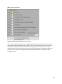
4.1.1 Control Panel VI
The Control Panel VI is the primary graphical interface for use in metering frequency fluctuations.
Figure 22. Control Panel VI user interface.
As seen in the main project GUI in figure 22, the user can select which serial port to connect on,
corresponding to the port they connected to the Arduino (either via mini-USB or RS232 connection).
Baud rate is set to 115200 as default and will cause errors if it is changed. The LabVIEW program
expects 1 byte to be read at a time and hence the data read rate has been set to 5ms so that it can
collect all the data at the port in time.
The data that is sent to the Arduino is shown in the ‘Sent Serial Message’ string indicator and the
data that are received back, including all handshake characters are displayed in the ‘Input from
Arduino Due’ string indicator.
Frequency data is displayed in real-time as it is collected from the Arduino and is plotted on the
Real-Time Frequency Value graph. The user may alter the time period they wish to display by
modifying the Time axis values. The Frequency axis scales itself proportionally to the input
information but this may be altered by the user.
The frequency change threshold input allows the user to select how much the frequency is allowed
to change from second to second in order to attempt to delete all outlier data that may be
generated due to multiple Arduino ISR’s running consecutively.
40
The user may select either Drift Logging Mode to log the Arduino clock jitter to a CSV file or
Frequency Logging Mode. Over and under frequency data is logged, maximum durations are stored
and a Boolean display lights up to indicate these conditions.
4.1.2 Supporting Functions
While these files are documented within their respective VI programs, this section attempts to give a
brief description of the purpose of each VI file that supports the Control Panel VI at run-time.
GPS_Week_and_Seconds.vi
This file provides the functionality of generating the GPS time in seconds since the start of the week
(Sunday 0000 24-Hour Time). The default parameters are UTC+8 (Perth Time), UTC Offset off. The
output type is a 32-bit signed integer.
GPS_Fix.vi
The GPS_Fix VI provides a GPS fix determination based on the GPGGA message output by the
Copernicus II module. The VI expects a GPGGA string message including both the ‘$’ start character
and the checksum at the end. The LabVIEW string library finds the separation index of the commas
located throughout the message and dissects the message based on these string index values into its
various components, such as UTC Time, GPS Fix Status, Latitude/Longitude and more. Output types
are dissected message strings and a Boolean value that determines whether the GPS has obtained a
satellite fix.
PadZeroes.vi
The PadZeroes VI takes a string input and replaces all spaces with a string value of 0. This VI is
primarily used to support the NMEA_Configuration VI file. The output type is a string.
NMEA_Configuration.vi
Figure 23. NMEA Configuration VI user interface.
The configuration VI shown in figure 23 allows the user to configure the NMEA packets for the
Trimble Copernicus II, prior to run-time on the Control Panel VI. All of the sentences listed in table 8
are able to be configured through this VI with practical defaults already set such as:
41
Receiver Configuration: 15° elevation mask to reduce ionospheric jitter, Land dynamics, WAAS
enabled (Even though WAAS corrections are not available in Australia [50], future implementations
of WAAS will allow the frequency meter to perform with even less jitter on the PPS output).
PPS Configuration: Only generate outputs if a GPS fix is available, 500ms pulse length, active HIGH,
10ns cable delay compensation due to standard SMA connector antenna.
Acquisition Sensitivity: Standard (lowest PPS jitter setting).
Serial Communications: 19200 Baud (Already the default for NMEA in the Arduino program).
Initial Position: GPS week and time are automatically generated by LabVIEW based on the system
time. Latitude and Longitude are set to the Engineering and Energy building location at Murdoch
University and altitude 10m above sea level. This location has to be within 100km of the true
location and within 5 minutes of the specified UTC time to allow the receiver to lock on as fast as
possible.
Reset Configuration: Hot Start, store user configuration to flash memory on reset/stand-by request,
wake up on activity on Port-B (NMEA IN).
Each of these sentences can be modified with minimal work by the user and the VI details any
comments relating to expected input format. The output type of all sentences is a string.
NMEA_Checksum.vi
This VI performs an 8-bit exclusive OR on all the ASCII byte value components of the literal string
input. The output type is string, created by taking the final exclusively OR-ed byte and converting it
to a string representation of the hexadecimal byte equivalent.
Figure 24. NMEA checksum generation illustration.
Figure 24 displays how a string called “Example” may be broken into its individual characters and
each character has a decimal or base-2 binary representation. When each of these binary values are
exclusively ORed together, another binary value is output, and this can be represented as a
hexadecimal value that is finally represented as a string in NMEA messages. This string is used for
error checking from and to the GPS receiver.
42
NMEA_Packet_Decoder.vi
Figure 25. NMEA Packet Decoder VI user interface.
The VI shown in figure 25 is similar to the NMEA_Configuration VI in it’s function because it is in
charge of generating an NMEA message. However this VI is separate because it is not focused on
initialisation sentences but instead is focused on allowing the user to select from an array of
message instruct the GPS module choices to generate the appropriate automated message at the
chosen rate. The receiver can configure all of the messages in figure 25, a number of chosen
messages or none.
43
4.2 Arduino
Two program files were created for use with the Arduino Due:
1. MFFM_Arduino.ino
2. QuantifyClockCycles.ino
Logging the Arduino’s clock drift can be done through the MFFM_Arduino program in addition to the
ability to modify this program to alternately send frequency data. The relevant LabVIEW
configurations have already been made, so choosing the right main loop function and relevant ISRs is
simple.
The QuantifyClockCycles program is detailed in the “PPS ISR Processing Time” sub-section below and
its primary purpose is to ascertain the number of clock cycles that elapse during ISR calls in order to
offset collected data values and bring the measurement trueness closer to the actual value.
4.2.1 PPS ISR Processing Time
The PPS time-collection is an ISR that is triggered by the rising edge of a digital pin connected to the
PPS output of a GPS receiver. The purpose of the ISR is to quantify the ISR’s processing time in order
to offset clock jitter data from the Arduino Due. The code for this can be seen in appendix A and a
structured flow-chart of the program is given:
Figure 26. ISR clock-cycle quantifying program.
44
The mean processing time for the SysTick->VAL storage call and the PPS GetRisingEdge() ISR were 7
clock cycles and 194.97 clock cycles respectively, with a standard deviation of ~0 on both. This time
corresponds to the execution cycles undertaken when a rising edge has occurred.
This translates to an offset of 2.321 µs for the PPS ISR and a final adjusted offset of 2.238 µs when
the clock cycles that SysTick->VAL calls require are factored in.
4.2.2 Alternate Microsecond Function Implementation
One significant factor in the design of the Arduino programs was the calls to the micros() function.
Micros() returns an unsigned 32-bit integer ‘time’ value upon each call equal to the number of
microseconds that have elapsed since the Arduino Due was turned on. This function had the issue of
gaining a millisecond during some ISR calls because the system timing ISR was not able to be called.
uint32_t micros( void )
{
uint32_t ticks ;
uint32_t count ;
SysTick->CTRL;
do {
ticks = SysTick->VAL;
count = GetTickCount();
} while (SysTick->CTRL & SysTick_CTRL_COUNTFLAG_Msk);
return count * 1000 + (SysTick->LOAD + 1 - ticks) /
(SystemCoreClock/1000000) ;
}
Figure 27. Previous Arduino library implementation of micros() [10].
The code in figure 27 was unsuitable for use in interrupts due to relatively frequent error of 1ms.
The user “stimmer” [51] submitted a more suitable micros function that does not suffer from the
SysTick register rollover issue, and this was implemented within the ISRs generated in the code.
Figure 28 provides the code submitted by stimmer and did not have any observed millisecond sized
fluctuations during any logging periods, thereby relieving the initially detected issue.
45
uint32_t micros( void )
{
uint32_t ticks, ticks2;
uint32_t pend, pend2;
uint32_t count, count2;
ticks2 = SysTick->VAL;
pend2
= !!((SCB->ICSR & SCB_ICSR_PENDSTSET_Msk)|
((SCB->SHCSR & SCB_SHCSR_SYSTICKACT_Msk))) ;
count2 = GetTickCount();
do {
ticks=ticks2;
pend=pend2;
count=count2;
ticks2 = SysTick->VAL;
pend2
= !!((SCB->ICSR & SCB_ICSR_PENDSTSET_Msk)|
((SCB->SHCSR & SCB_SHCSR_SYSTICKACT_Msk))) ;
count2 = GetTickCount();
} while ((pend != pend2) || (count != count2) || (ticks < ticks2));
return ((count+pend) * 1000) +
(((SysTick->LOAD - ticks)*(1048576/(F_CPU/1000000)))>>20) ;
/* this is an optimization to turn a runtime division into two
compile-time divisions and a runtime multiplication and shift, saving a
few cycles */
}
Figure 28. New interrupt functioning implementation of micros() [51].
4.2.3 Frequency Metering
The metering program on the Arduino is configured to allow either manual or automatic setup. In
addition to this, the program only needs two minor modifications to run in jitter logging mode,
where the Arduino will log time based on an external interrupt trigger such as a GPS PPS signal. After
the Arduino finishes setup, the output is periodic, based on the PPS generated ISR.
Figure 29 displays the routine the Arduino undertakes for normal frequency metering operation. The
stages are segmented and interdependent with LabVIEW to progress to the next stage if a LabVIEW
connection is detected.
46
Figure 29. Arduino frequency metering program flow-chart.
In the declaration and initialisation of variables, all the variables that are used throughout the
program (including in ISRs) are specified. Variables that may have their value changed within an ISR
are set as volatile. This is done by writing the volatile keyword before the variables data type is
declared. The advantage of this is that the correct value will be brought up when the variable is
called as it is stored in RAM memory rather than a storage register.
Functions were developed within the program to both reduce the overhead with re-writing the same
code and to make the code more readable. In a brief summary, the functions perform the following
tasks:
47
•
•
•
•
•
•
•
•
•
•
HWCDelay() – void type, returns nothing. Executes delay() function for a specified
millisecond value. Used to allow HardWare Configuration packets to take place in the
Trimble Copernicus II GPS receiver.
NMEA_Packet_Checker() – void type, returns nothing. Primarily used for debugging, allows
manual input of NMEA packet strings through Serial0 to verify the reply packet is received
and valid.
GetRisingEdge() – void type, returns nothing. ISR function. Generated when a PPS rising edge
is detected on digital pin 8. Holds value from micros() function when the interrupt is
generated.
ClearSerial#() – void type, returns nothing. There are 4 ClearSerial#() functions, where # is
replaced by 0, 1, 2 and 3, corresponding to the 4 Serial UARTs on the Arduino. This function
wipes all buffered data on the UARTs.
NMEA_Response() – short int type, returns -1, 0, 1 or 2. Verifies the NMEA packet that was
sent to the Copernicus II was correct. Returns -1 for unknown message, returns 0 for invalid
packet, returns 1 for valid packet and returns 2 for response time-out.
GetNMEA() – void type, returns nothing. Gets an NMEA message from LabVIEW and stores it
in a buffer.
SendNMEA() – void type, returns nothing. Sends the buffered NMEA message to the
Copernicus II and appends the carriage return and line feed characters.
Serial#_Protocol_Request() – void type, returns nothing. # is replaced by 0 or 2,
corresponding to the active Arduino to LabVIEW serial line. Requests the NMEA packets
from LabVIEW sequentially and communicates in a custom protocol.
Reset_Copernicus_Comms() – void type, returns nothing. Changes the Copernicus II baud
rate to the original 4800bps.
GetFrequency() – void type, returns nothing. ISR function. Generated when a pulse is
generated on digital pin 9 by the periodic pulse generator that has the same frequency as
the mains supply.
The Arduino will wait for 10 seconds to elapse before it enters manual configuration mode. In
automatic setup mode, a protocol has been developed to allow the Arduino and LabVIEW programs
to communicate NMEA packet data for initialisation of the Trimble Copernicus II GPS receiver. The
Arduino will poll LabVIEW for the NMEA packets it requires. The NMEA packets for the EM406-A
however will always need to be manually entered if it is chosen as the PPS ISR generating GPS
receiver, as the Trimble Copernicus II GPS receiver is configured for default settings.
The program will wait for the periodic output GGA message to confirm the GPS has a fix. The
number of satellites required to make the GPS fix valid will depend on whether the Copernicus II is
operating in stationary mode or an alternative dynamic, such as Land, Sea or Air. In stationary mode,
only one satellite is required to get a time signal fix but the jitter increases from ±60ns to ±350ns
[33]. In all other modes the jitter is at the nominal ±60ns data sheet specified value [33]. As soon as
the GPS fix is valid, the appropriate interrupts are attached and the main loop is run.
The main loop is fairly simple, comma separated data (Pulses Counted, Gating Error at Start, Gating
Error at End) is printed to the active serial line and stored to the SD card as backup.
48
5 Timing Precision
Timing precision results were generated over 48 hours to ensure the data could be analysed over a
cyclical period to determine if the KX-7 crystal’s timing jitter varied periodically.
Temperature (°C)
Min
Max
29/10/2013
13
31
30/10/2013
18
37
31/10/2013
14
26
01/11/2013
14
27
02/11/2013
16
29
Table 11. Temperature data for the jitter logging time interval.
Date
Mean
22
28
20
20
22
The temperature data in table 11 is of importance because it can be compared to the variations in
jitter on the KX-7 crystal, since temperature will have the greatest effect.
5.1 Arduino Frequency Stability Data
Performance tests were created to quantify the clock drift of the Arduino Due’s 12MHz KX-7 Quartz
Crystal.
𝑝𝑝𝑚 =
106 ×∆𝑓
𝑓
(4)
To attempt to correlate the logged data to a similar standard, the EM406-A and the Trimble
Copernicus II GPS receivers both provided a PPS signal as a reference timer on the Arduino Due.
Deviation from this PPS signal would come from the crystal oscillator’s frequency jitter and a
significantly smaller portion of this deviation is quantified as the PPS signal jitter itself.
5.1.1 Clock Drift Relative to Trimble Copernicus II
The clock drift of the Arduino was logged through a 48 hour PuTTY session into a comma separated
value file. It’s also possible to log the clock drift of the Arduino now with the latest implementation
of the LabVIEW programs.
Mean (µs)
999993.2195
Max Value Mean (µs)
Min Value Mean (µs)
Standard Deviation Mean (µs)
999995
999990
0.613217
Table 12. PPS triggered Arduino 1-second timing interval data (Copernicus II PPS source).
From the mean value in table 12, the mean jitter can be calculated on the Arduino for the 48 hour
period. The mean error value is calculated at -6.7805 ppm with a standard deviation of ±0.613
49
around the mean value, corresponding to the crystal’s jitter. By accounting for the ISR processing
time in the Arduino code, this mean error is reduced to -4.5425ppm. No compensation is made for
the jitter contribution made by the Copernicus II as it is assumed that while the PPS jitter is ±60ns, its
mean value is sufficiently close to 0 to make it negligible.
The Copernicus II GPS receiver exhibited a 100% up-time during the data logging session with only 4
successive timing outliers that had to be removed due to incorrect timing values being recorded.
Appendix 4 lists the data collection dates and times and what packets were used to initialise each
GPS receiver.
Figure 30. Histogram of PPS generated time intervals on the Arduino Due (Copernicus II PPS source).
Figure 30 displays the recorded timing distribution in a histogram. The time interval data appears to
largely be centered around 999,993µs, with mostly ±1µs sway to each side. The initial assumption
was that the timing jitter would be largely erratic given the nature of the ppm specifications found in
literature, however this data implies otherwise.
50
Figure 31. Arduino 48 hour mean-centered jitter graph (Copernicus II PPS source).
Figure 31 above displays how the Arduino’s jitter changes over the 48 hour logging period relative to
the PPS signal the Copernicus II GPS receiver provides. The initial aim was to allow the ambient
temperature to naturally change and directly affect the Arduino’s timing jitter. Unfortunately, while
the location where this data was collected was suitable for frequency logging due to excellent GPS
signal reception and the ability to leave the laptop running for 48 hours to collect the data, airconditioning was turned on at 9AM each day and skewed the results. This is displayed by the fact
that the jitter is primarily positive around the mean value, indicating a cooler environment when
compared to the data collected in 5.1.2.
51
Figure 32. Arduino 48 hour TIE graph (Copernicus II PPS source).
The TIE graph in figure 32 attempts to illustrate the low long-term effect that the temperature had
on timing jitter of the Arduino was negligible with relatively small temperature variations. The R2
value is very high, indicating a high data correlation to the linearly fit trend-line. After 172,800
seconds (48 hours), the TIE accumulated to 799.08ms, or an average of 399.54ms lost to the
Arduino’s timing offset per day. This value is largely based on the mean error from the PPS signal
time and is minimally affected by the clock’s jitter.
52
5.1.2 Clock Drift Relative to GlobalSat EM406-A
The EM406-A provided a PPS timing source for the Arduino in an ambient temperature affected
environment. Air-conditioning was kept off to prevent artificial modification to the jitter logging
data. A PuTTY client recorded the 48 hour session, similarly to section 5.1.1.
Mean (µs)
Max Value (µs)
Min Value (µs)
Standard Deviation (µs)
999993.8166
999995
999992
Table 13. PPS triggered Arduino 1-second timing interval data (EM406-A PPS source).
0.540911
The mean error value was logged at -6.1834 ppm over the 48 hour logging session with jitter
analysed from the standard deviation value of ±0.541ppm around the mean error. The PPS ISR
compensated mean error was -3.9454ppm.
Figure 33. Histogram of PPS generated time intervals on the Arduino Due (EM406-A PPS source).
The histogram data in figure 33 displayed a similar result to section 5.1.1 with a large distribution
being centered around one value (999,994) and mostly a ±1µs jitter long-term about this value.
Similarly, no erratic variations in Arduino timing jitter were detected.
53
Figure 34. Arduino 48 hour mean-centered jitter graph (EM406-A PPS source).
In an ambient temperature affected environment, the Arduino’s jtter around its mean timing value
displayed a very similar start to the data in 5.1.1 but was dissimilar in the fact that it appeared
similar to a sinusoidal waveform, indicating a periodically repeating nature. The temperature data in
the start of section 5 indicates that over the 48 hour period, a repeating set of data should appear
over the first 48 hours and a larger trough should be displayed due to the highest temperature data
being on the final day of the recording. This can be seen by the trough around the 138381 second
mark dipping lower than the previous trough. While observations can be made upon this data,
improvements could be made in the future to simulatenously log ambient temperature and attempt
to correlate the two sets of data. Overall, a cyclical nature in the Arduino crystal jitter is observed
when ambient temperature is not affected by household climate control systems such as airconditioning.
54
Figure 35. Arduino 48 hour TIE graph (EM406-A PPS source).
A final TIE for the EM406-A based set of data is generated and can be seen in figure 35. The TIE is
accumulated to 672.64ms over the 48 hour period. The data set again gives a linear trend with a very
high R2 value, indicating the data in the trend-line fit correlates highly. 336.32ms are lost by the
Arduino on average in this set of data per day, 15.04% less than the time lost in the Copernicus II
data set. This corresponds to and average of -3.89ppm, well within the ±30ppm specification given
by the KX-7 crystal’s manual [24].
55
6 Frequency Meter
With a quantified Arduino timing bias, frequency metering was able to be performed. Similar to
section 5, a 48-hour set of data was obtained on the mains supply’s frequency to determine if the
data was cyclical and whether the frequency varied as expected.
6.1 Setup
Prior to logging the frequency data, setup needed to be performed in the LabVIEW program settings,
the Arduino program MFFM_Arduino.ino and the physical connections needed to be created, as
shown in figure 36.
Figure 36. Physical frequency meter setup.
56
6.1.1 Hardware Components
A 3V SMA-connect antenna was connected to the SMA male connector on the Trimble Copernicus II
to increase signal reception. A 3.3V and GND rail were connected on the breadboard to provide
power to the Copernicus II module. The connections for the Copernicus II are shown in figure 32,
with the active connections bolded.
LNA
SMA Connector
Reserved 1
OPEN
Trimble
SHORT
Copernicus II
Reserved 2
63530-00
GPS
VBATT – 3.3V
XRST – 3.3V
VCC – 3.3V
GND – 0V
XSTBY – 3.3V
Figure 37. Trimble Copernicus II connected pins diagram.
Reserved 7
Reserved 6
TX-B (NMEA)
TX-A (TSIP)
Reserved 5
RX-A (TSIP)
RX-B (NMEA)
PPS
Reserved 4
Reserved 3
The RS232 shield has digital pin 16 and 17 connected to the Arduino as soon as the shield is
connected, allowing communication instantly. The Arduino’s 5V rail powers the MAX232N DIP
module. The mains supply can be connected in any manner to the green screw terminal on the pulse
generation shield and is not polarity sensitive. The shield stacking hierarchy is as follows:
Arduino Due (bottom) -> RS232 Shield -> Pulse Generation Shield -> SD Card Shield (top)
The SD card shield connections are as outlined in table 5.
6.1.2 Program Parameters
To run the frequency metering correctly, several program files must be configured properly.
In the Arduino environment’s MFFM_Arduino program there exist two interrupt functions named
GetRisingEdge(). One is used for logging relative clock jitter on the Arduino, as outlined by the results
in section 5. The alternative is used for frequency metering which is relevant to this section. Figures
38 and 39 display the GetRisingEdge() ISR function code. The code in figure 38 is used for timing
precision analysis while the code in figure 39 has been adapted for use in metering the mains
frequency.
57
void GetRisingEdge() {
PrevMicros = NewMicros;
NewMicros = micros();
EdgeChanged = true;
++countedges;
}
Figure 38. PPS ISR for timing precision analysis.
void GetRisingEdge() {
PPS_Micros = micros();
Final_Gap = PPS_Micros - PulseTime;
PPS_Started = true;
EdgeChanged = true;
PulsesCounted = PulseCount;
PulseCount = 0;
return;
}
Figure 39. PPS ISR for frequency metering.
To change between the two functions, simply comment out the function that is redundant by
wrapping the start with the /* characters and the end of the redundant function with the */
characters. This approach will be also used in the main loop
Two sets of if statements exist within the main body, as shown in figure 40.
/*if ( EdgeChanged == true ) {
EdgeChanged = false;
Serial.print(NewMicros);
Serial.print(",");
Serial.print(PrevMicros);
Serial.print(",");
Serial.println(countedges);
} */
if (EdgeChanged == true) {
EdgeChanged = false;
Serial.print(PulsesCounted);
Serial.print(",");
Serial.print(Initial_Gap);
Serial.print(",");
Serial.print(Final_Gap);
}
Figure 40. Statements given in main Arduino loop.
58
The commented out code in the main loop pertains to the jitter analysis variables. The rest of the
code is used in frequency metering. Further comments pertaining to this are available within the
program’s comments, found in Appendix A.
The LabVIEW setup involves setting up three VI files – Control Panel, NMEA_Configuration and
NMEA_Packet_Decoder. The rest of the project library will provide support functions and must not
be modified.
The Control Panel is relatively simple to set up, simply select the ‘Frequency Logging Mode’ button.
If the ‘Drift Logging Mode’ button is concurrently selected, Frequency Logging will take precedence.
The operator must specify the location of where you want to save the data set and append the file
name with the ‘.csv’ extension. The frequency change threshold value on the Control Panel is
recommended to be set at 0.2Hz but this may be changed depending on the range of outlier data
the user may experience. Results on the Arduino indicated that any change over ±0.2Hz tends to be
an outlier with typical values averaging around ±1Hz.
The NMEA_Configuration file allows the user to change the NMEA packets in order to speed up the
Copernicus II initialisation time and modify its functionality. It is recommended that the values be
left as default for the most part. The user should primarily use this VI to insert their GPS coordinates
in order to obtain a GPS fix faster. As long as the coordinates are within 100km of the correct
location, they will be valid. If poor signal reception is experienced, it is possible to change the
receiver to High Sensitivity Mode. If a lock onto less than 4 satellites is established for a long period,
the NMEA configuration can be changed to ‘Stationary’ dynamic rather than Land, Sea or Air. This
provides a PPS time base from 1 satellite but at the cost of increased PPS jitter.
The NMEA_Packet_Decoder may provide more automated GPS messages than the GGA message
that is typically used. The user will have to modify the LabVIEW or Arduino program(s) to parse this
data, depending on it’s intended use. It is recommended that the default settings are used and the
GGA message is always selected for output.
Following these setup steps, the programs are ready to run if a physical connection to the Arduino is
established.
59
6.2 Performance Results
Figure 41. 48 Hour frequency log graph.
Figure 41 demonstrates the overall 48 hour mains supply frequency data set that the Arduino
logged. The mean data set value was 50.0001Hz with a standard deviation of 0.0263Hz. This is as
expected as the grid frequency should not vary greatly in order to maintain nominal values.
Contingency
Day
Start Time
Finish Time
Total Duration
Under-frequency
Sunday
02:44:44 AM
02:46:39 AM
1 min, 55
(Event 1)
seconds
Under-frequency
Monday
05:29:11 PM
05:32:45 PM
3 min, 34
(Event 2)
seconds
Table 14. Under-frequency events detected during frequency meter performance tests.
Two under-frequency events were detected on the grid. The first under-frequency event lasted a
short duration at the times given in table 14. It is likely that the grid had very few loads connected at
this time compared to the amount connected during the day and a large number of loads connecting
to the grid at this early hour affected the grid in an unexpected way, but this could only be
confirmed by obtaining frequency data from a more accurate and verified source.
The second under-frequency event was after typical working day hours on a Monday and is likely
caused by a very large number of loads connecting to the grid suddenly, thereby slowing down the
large generators that maintain the grid frequency. The recovery times on both under-frequency
events were well within the 15 minute specification for return to nominal grid frequency.
60
Figure 42. Under-frequency Event 1 graph.
The first under-frequency event can be seen in figure 42. The data seems to dip and rise over the
course of 12 seconds from 50Hz to below 49.8Hz and then to 49.85Hz. Successive dips in the grid
frequency are minor and end 1 minute, 55 seconds after the initial dip below the grid frequency.
Figure 43. Under-frequency Event 2 graph.
The under-frequency event displayed in figure 43 dips very quickly (over the course of seconds),
similar to the under-frequency event in figure 42. The initial dip similarly experiences slight swing
back closer to nominal frequency and then gradually recovers to the nominal value. The data in
event 2 was expected at the time it was recorded and the waveform, while slightly noisy,
demonstrates that minor frequency fluctuations are be detected on the mains supply line.
61
7 Recommendations and Future Improvements
The timing source jitter analysis for the KX-7 quartz crystal was performed on two GPS receivers that
induced their own jitter into the measurements as well, thereby reducing the precision of the
analysis. To improve this, a higher standard of timing such as an atomic standard could be used to
analyse the timing jitter directly against. As atomic standards have very low jitter (on the order of
parts per billion), they would be a suitable candidate.
Data collected on the Arduino for timing jitter analysis was not monitored closely with respect to
temperature variations. While it can be inferred that temperature had an effect on the frequency
stability of the Arduino’s crystal oscillator based on theory, quantifying the scale of change in jitter
across different temperature ranges would allow a temperature dependent model to be developed
for the crystal, therefore allowing the crystal to be used without an external standard providing a
time-base for the MCU as its jitter could be quantified at any time based on a temperature sample.
External effects such as pressure, aging and other effects defined in section 2.1.3 could also be
considered.
The GPS pulse-per-second signal was considered in the jitter analysis of this project but was not able
to be quantified due to the length of time required to log the signal jitter, the very low short-term
jitter (order of nanoseconds) and the shared phase relationship between the two GPS receivers. By
quantifying the actual jitter of both GPS receivers’ PPS outputs, experimentally derived corrections
can be made to the measurements made on the Arduino’s jitter instead of relying upon data sheet
specifications.
The Arduino Due is an excellent MCU in today’s market, offering an excellent sampling speed, low
cost, excellent clock rate and considerably large amount of SRAM/Flash memory. In the future
however, improved MCU models will be released that operate at the same clock rate or higher with
even more powerful specifications. The main improvement of a new MCU would be a faster
sampling rate, as right now the resolution is set at a maximum of 1µs. This is effective for long-term
jitter logging but for analysing very small short-term changes in clock jitter such as that claimed by
GPS receivers, this is much too high. Hence it is recommended that hardware improvements are
performed when a cost effective upgrade is available.
Among other hardware upgrades, improved filtering could be designed to replace the first-order
low-pass filter on the Arduino frequency detection shield. A second-order or better band-pass filter
could be created to attenuate signals outside the nominal range, but generally an improved low-pass
filter design should be just as good as the mains frequency is relatively low. The transistor amplifier
circuit on the frequency detection shield performs well and detects the frequency of the mains
supply but could also be improved by designing a zero-crossing detector circuit that performs with
minimal propagation delay and is reliable.
Lastly, the data is currently transmitted either only to an SD card or directly to a PC terminal. A GSM
shield would add wireless data collection capability and could send data periodically to a database to
remove the need for a physical connection to log the data. This would enable the user to simply
attach the instrument to a power socket, let it record for as long as is needed and return to obtain
the frequency meter when the measurement point is no longer required.
62
8 Conclusion
The developed frequency meter achieved all the primary objectives and all set minor objectives. The
Arduino Due MCU crystal oscillator was found to be performing well within it’s data sheet timing
jitter specification, allowing it to perform well in most applications where a stable time base is
critical. The GPS timing implementations did not vary greatly in the resultant Arduino timing jitter
data sets, inferring the GPS signal jitter is negligible at the Arduino Due’s sampling rate specification.
The studies undertaken in this thesis were broad and developed necessary engineering skills. A
broad range of learning outcomes were gained such as time management, task prioritisation,
physical and theoretical electronic design implementations and their respective limitations,
hardware cost-benefit margin analysis, awareness of available software implementations, project
schedule management and the ability to work independently to a stakeholder’s project
specifications.
The frequency meter was able to detect the mains frequency at a specification higher than the set
objective of metering mHz-level fluctuations on the grid. By utilising an MCU with a high sampling
rate, frequency changes were detectable on the order of µHz based on the timing jitter results found
in section 5. The system had the limitation of noisy frequency readings at the µHz resolution
however. This may be due to mains supply noise triggering the pulse generation shield at slightly
incorrect times due either to mV-level variations on the grid or noise induced by the mains adapter.
Future improvements in regards to this and other recommendations have been outlined in section 7.
63
9 References
[1] International Organisation for Standardisation, “ISO 5725-1:1994,” 2012. [Online]. Available:
http://www.iso.org/iso/catalogue_detail.htm?csnumber=11833. [Accessed 09 September
2013].
[2] International Organisation for Standardisation, “ISO 3534-1:2006,” 2010. [Online]. Available:
http://www.iso.org/iso/catalogue_detail.htm?csnumber=40145. [Accessed 09 September
2013].
[3] Wikipedia, “Accuracy and Precision,” 28 October 2013. [Online]. Available:
http://en.wikipedia.org/wiki/Accuracy_and_precision. [Accessed 29 October 2013].
[4] Royal Society of Chemistry, “AMC Technical Brief,” September 2003. [Online]. Available:
http://www.rsc.org/images/terminology-part-1-technical-brief-13_tcm18-214863.pdf.
[Accessed 9 September 2013].
[5] Wikipedia, “Frequency Measurement,” 2013. [Online]. Available:
http://en.wikipedia.org/wiki/Frequency#Measurement. [Accessed 24 October 2013].
[6] J. Carr, “Radio Receivers,” in RF Components and Circuits, Elsevier Newnes, 2002, pp. 41-46.
[7] Wikipedia, “Aliasing,” 2013. [Online]. Available: http://en.wikipedia.org/wiki/Aliasing.
[Accessed 24 October 2013].
[8] B. A. Olshausen, “Aliasing,” 10 October 2000. [Online]. Available:
http://redwood.berkeley.edu/bruno/npb261/aliasing.pdf. [Accessed 28 October 2013].
[9] Hewlett Packard, “Fundamentals of Quartz Oscillators,” 3 September 2000. [Online]. Available:
http://literature.agilent.com/litweb/pdf/5965-7662E.pdf. [Accessed 1 August 2013].
[10] Arduino, “Arduino - ArduinoBoardDue,” 23 October 2012. [Online]. Available:
http://arduino.cc/en/Main/arduinoBoardDue. [Accessed 29 July 2013].
[11] GlobalSat, “EM406-A Product User Manual,” GlobalSat Technology Corporation, 16 February
2010. [Online]. Available: http://elmicro.com/files/sparkfun/em406a_ug.pdf. [Accessed 20
August 2013].
[12] SparkFun Electronics, “Copernicus II DIP Module,” 2013. [Online]. Available:
https://www.sparkfun.com/products/11858. [Accessed 17 August 2013].
[13] D. L. Mills, “Network Time Protocol (Version 3) - Specification, Implementation and Analysis,”
March 1992. [Online]. Available: http://www.ietf.org/rfc/rfc1305.txt. [Accessed 9 October
2013].
64
[14] D. L. Mills, “Network Time Protocol Version 4: Protocol and Algorithms Specification,” June
2010. [Online]. Available: http://tools.ietf.org/html/rfc5905. [Accessed 14 October 2013].
[15] HyperPhysics, “Atomic Clocks,” 27 April 2009. [Online]. Available: http://hyperphysics.phyastr.gsu.edu/hbase/acloc.html. [Accessed 5 November 2013].
[16] Wikipedia, “Radio Clocks,” 27 August 2013. [Online]. Available:
https://en.wikipedia.org/wiki/Radio_clock. [Accessed 8 October 2013].
[17] The Hindu Business Line, “US scientists build world’s most precise clock,” 23 August 2013.
[Online]. Available: http://www.thehindubusinessline.com/news/international/us-scientistsbuild-worlds-most-precise-clock/article5051703.ece. [Accessed 8 October 2013].
[18] Wikipedia, “Rubidium Standard,” 17 August 2013. [Online]. Available:
https://en.wikipedia.org/wiki/Rubidium_standard. [Accessed 5 November 2013].
[19] Bureau International des Poids et Mesures, “BIPM: Bureau International des Poids et Mesures,”
2013. [Online]. Available: http://www.bipm.org/. [Accessed 8 October 2013].
[20] International Bureau of Weights and Measures, “Time Signals,” March 2013. [Online]. Available:
ftp://ftp2.bipm.org/pub/tai/scale/timesignals.pdf. [Accessed 8 October 2013].
[21] BIPM, “Time Signals,” March 2013. [Online]. Available:
ftp://ftp2.bipm.org/pub/tai/scale/timesignals.pdf. [Accessed 8 October 2013].
[22] L. Tetley and D. Calcutt, Electronic Navigation Systems, Woburn: Butterworth-Heinemann,
2001.
[23] M. A. Lombardi, “How Accurate is a Radio Controlled Clock?,” Horological Journal, p. 4, 2010.
[24] Geyer Quartz Technology, “Geyer KX-7 Quartz Crystal,” 19 October 2012. [Online]. Available:
http://www.geyer-electronic.de/uploads/tx_userartikelfrequenz/GEYER-KX-7_01.pdf.
[Accessed 17 October 2013].
[25] B. A. Forouzhan and F. Mosharraf, “Computer Networks - A Top-Down Approach,” in Physical
Layer and Transmission Media, New York, McGraw-Hill, 2012, pp. 548-560.
[26] International SEMATECH Manufacturing Initiative, “Using Network Time Protocol (NTP):
Introduction and Recommended Practices,” 28 February 2006. [Online]. Available:
http://www.sematech.org/docubase/document/4736aeng.pdf. [Accessed 16 October 2013].
[27] J. Burch, K. Green, J. Nakulski and D. Vook, “Verifying the Performance of Transparent Clocks in
PTP Systems,” in International IEEE Symposium on Precision Clock Synchronisation for
Measurement, Control and Communication, Brescia, 2009.
[28] G. D. Krebs, “GPS-2A (Navstar-2A),” 27 January 2013. [Online]. Available:
65
http://space.skyrocket.de/doc_sdat/navstar-2a.htm. [Accessed 5 Novermber 2013].
[29] Lockheed Martin, “U.S. Air Force Awards Lockheed Martin GPS III Flight Operations Contract,”
31 May 2012. [Online]. Available: http://www.lockheedmartin.com/us/news/pressreleases/2012/may/0531-ss-gpsIII.html. [Accessed 18 August 2013].
[30] Lockheed Martin Corporation, “GPS III - The Next Generation Global Positioning System,” 2011.
[Online]. Available:
http://www.lockheedmartin.com.au/content/dam/lockheed/data/space/documents/gps/GPSII
I_FactSheetFINAL1.pdf. [Accessed 11 November 2013].
[31] U.S. Department of Defense, “DoD Permanently Discontinues Procurement Of Global
Positioning System Selective Availability,” 18 September 2007. [Online]. Available:
http://www.defense.gov/releases/release.aspx?releaseid=11335. [Accessed 19 August 2013].
[32] Kowoma, “Sources of Error in GPS,” 2013. [Online]. Available:
http://www.kowoma.de/en/gps/errors.htm#atmospheric. [Accessed 11 October 2013].
[33] Trimble, “Copernicus II GPS Receiver - Reference Manual,” 2 September 2011. [Online].
Available: https://dlnmh9ip6v2uc.cloudfront.net/datasheets/Sensors/GPS/63530-10_RevB_Manual_Copernicus-II.pdf. [Accessed 17 August 2013].
[34] Standards Australia, “AS 60038-2012 - Standard Voltages,” SAI Global Limited, Sydney, 2012.
[35] Western Power, “Technical Rules,” 23 December 2011. [Online]. Available:
http://www.westernpower.com.au/documents/aboutus/accessarrangement/2011/WE_n6800
863_v9E_TECHNICAL_RULES_OF_23_DECEMBER_2011.pdf. [Accessed 29 July 2013].
[36] Atmel, “AT91SAM ARM-based Flash MCU,” 9 September 2012. [Online]. Available:
http://www.atmel.com/Images/doc11057.pdf. [Accessed 21 August 2013].
[37] Arduino, “Arduino - Compare,” 2013. [Online]. Available:
http://arduino.cc/en/Products.Compare. [Accessed 8 October 2013].
[38] Freescale Semiconductor, Inc, “Microcontrollers,” 2013. [Online]. Available:
http://www.freescale.com/webapp/sps/site/homepage.jsp?code=PCMCR01. [Accessed 8
October 2013].
[39] Microchip Technology Inc., “Microchip MCUs,” 2013. [Online]. Available:
http://www.microchip.com/pagehandler/en-us/products/picmicrocontrollers. [Accessed 8
October 2013].
[40] Freescale Semiconductor, “HC11 Microcontrollers,” 07 2005. [Online]. Available:
http://www.freescale.com/files/microcontrollers/doc/data_sheet/M68HC11E.pdf. [Accessed 2
November 2013].
66
[41] Arduino, “Arduino - FAQ,” 2013. [Online]. Available: http://arduino.cc/en/Main/FAQ. [Accessed
9 October 2013].
[42] Creative Commons, “Creative Common - Attribution Share-Alike 3.0 Australia,” 2013. [Online].
Available: http://creativecommons.org/licenses/by-sa/3.0/au/. [Accessed 9 October 2013].
[43] Free Software Foundation, “GNU Lesser General Public License,” 29 June 2007. [Online].
Available: http://www.gnu.org/licenses/lgpl.html. [Accessed 9 October 2013].
[44] D. Ibrahim, “Accurate Measurement of the Mains Electricity Frequency,” in International
Conference on Electrical and Electronics Engineering, Bursa, 2011.
[45] CADSoft, “Eagle 6.5.0 Download Page,” CADSoft USA, 7 August 2013. [Online]. Available:
http://www.cadsoftusa.com/download-eagle/?language=en. [Accessed 13 August 2013].
[46] Multicomp, “BC547B - General Purpose Transistor,” 12 May 2008. [Online]. Available:
http://www.farnell.com/datasheets/410427.pdf. [Accessed 2 October 2013].
[47] OnShine, “ONSHINE G.P.S. Antenna ANT-555 (GPS Active Antenna),” 1 June 2006. [Online].
Available: http://php2.twinner.com.tw/files/onshine/ANT555-2006-NEW.pdf. [Accessed 17
October 2013].
[48] GPS Source, “Calculating the propagation delay of coaxial cable,” 25 January 2011. [Online].
Available: http://www.gpssource.com/files/Cable-Delay-FAQ.pdf. [Accessed 17 October 2013].
[49] National Instruments, “LabVIEW System Design Software,” National Instruments, 2013.
[Online]. Available: http://www.ni.com/labview/. [Accessed 29 July 2013].
[50] GPS Oz, “WAAS,” May 2008. [Online]. Available: http://www.gpsoz.com.au/WAAS.htm.
[Accessed October 2013].
[51] stimmer, “GitHub,” April 2013. [Online]. Available:
https://github.com/arduino/Arduino/pull/1388/files. [Accessed 16 October 2013].
[52] M. P.J., “Relative timing characteristics of the one pulse per second (1PPS) output of three GPS
receivers,” in The 6th International Symposium on Satellite Navigation Technology Including
Mobile Positioning & Location Services, Melbourne, 2003.
[53] K. Ozsoy, A. Bozkurt and I. Tekin, “Indoor positioning based on global positioning system
signals,” Microwave and Optical Technology Letters, vol. 55, no. 5, pp. 1091-1097, 2013.
[54] Economic Regulation Authority, “Electricity Industry (Network Quality and Reliability of Supply)
Code 2005,” 6 December 2006. [Online]. Available:
http://www.era.wa.gov.au/cproot/2372/2/D04%20Electricity%20Industry%20%28Network%20
Quality%20and%20Reliability%20of%20Supply%29%20Code%202005.pdf. [Accessed 19 August
2013].
67
Appendices
Appendix A – Arduino Program
See attached folder named MFFM_Arduino
Appendix B – LabVIEW Program
See attached folder named MFFM_LabVIEW
Appendix C – Referenced Material
See attached folder named MFFM_References
Appendix D –Logging Session Data
Session Data for Jitter Logging
Trimble vs Arduino
29/10/2013 – 7:08 PM Logging Started
29/10/2013 – 7:08 PM First Fix
31/10/2013 – 7:10 PM Finish
Used NMEA Packets:
$PTNLSPS,2,5000000,0,0000000*51
$PTNLSFS,S,0*23
$PTNLSPT,019200,8,N,1,4,4*1C
$PTNLSKG,1764,241680000,3203.96635,S,11550.22761,E,00010*52
$PTNLSCR,,15,,,,0,1,,1*5C
68
Session Data for Jitter Logging
EM406A vs Arduino
31/10/2013 – 7:16 PM Logging Started
31/10/2013 – 7:17 PM First Fix
02/11/2013 – 7:20 PM Finish
Used NMEA Packets:
$PSRF100,1,19200,8,1,0*38
$PSRF105,1*3E
$PSRF103,00,00,01,01*25
$PSRF104,-32.066142,115.837122,10,96000,142774,2787,12,1*34
Session Data for Frequency Logging
Trimble Copernicus II PPS source on Arduino Due MCU
Start: 12:19PM 10/11/2013
Finish: 1:00pm 12/11/2013
Initialisation and PPS Packets:
$PTNLSKG,1766,087588000,3203.96635,S,11550.22761,E,00010*53
$PTNLSPS,2,5000000,1,10*51
All other packets were LabVIEW default settings.
All logged data can be found in the folder MFFM_Logged_Data
69
Appendix E – Annotated Bibliography
Fundamentals of Quartz Oscillators [9]
This document covers the natural and induced effects of clock sway in crystal oscillators. The varying
effects of time, temperature, natural forces (gravity, pressure), voltage and other factors are
analysed on three types of crystal oscillators – Room Temperature, Temperature Controlled and
Oven Controlled. The analysis provides a useful measure of the time interval at which the clocks
should be disciplined to stay true to a more precise time source. This study is directly applicable to
the measuring MCU (Arduino Due) as it uses an on-board crystal oscillator to keep track of time
which is subject unwanted clock sway effects over longer periods of time.
Relative timing characteristics of the one pulse per second (1PPS) output
pulse of three GPS receivers [52]
Three GPS receivers are analysed to determine the confidence associated with the precision of the
Pulse-Per-Second output of each. As atomic clocks are extremely expensive and difficult to obtain,
the author used a scientific-grade GPS as the reference clock which specified a much more precise
PPS deviation compared to the other two GPS receiver units. The clock deviation of the other two
GPS units was measured relative to the reference clock. Statistical analysis must be performed to
determine the trueness of the “disciplined clock” in this thesis. This paper provides an understanding
of what type of analyses must be performed (Allan Deviation excluded).
Accurate measurement of the mains electricity frequency [44]
The author presents a cost-effective solution to metering the grid frequency. This paper presents a
similar methodology wherein a PIC MCU is fed a digital pulse generated by a zero-crossing detector
circuit and counts the time between the pulses to determine the frequency. It also discusses
methodology to increase accuracy in obtaining the correct frequency and is highlights the drawbacks
of particular solutions such as counting the number of pulses in a second window. However this
method is not clock-disciplined but does give insight into the type of electronics that require
development.
Electronic Navigation Systems [22]
This book covers the different factors that affect radio signals at various frequencies and while
providing an introductory chapter to radio signalling, it also covers Satellite Navigation systems like
GPS [16]. Excellent explanations are given for the various effects that affect GPS such as atmospheric
effects, noise, operating frequency and others. This allows quantification of the effects that generate
systematic error in clock synchronisation.
70
Trimble Copernicus II GPS Receiver - Reference Manual [33]
This document contains all the data specifications for the Copernicus II GPS module except the clock
accuracy when a PPS fix is not obtained. NMEA packet configuration is given for this particular unit
[10] as a certain configuration must be running for both demonstration purposes and setup/testing.
Additionally this manual provides all the technical specifications and while lacking a set-up diagram
relevant to the Copernicus II DIP module, it infers enough to be able to connect it safely and for
reliable operation.
Indoor positioning based on global positioning system signals [53]
This paper analyses the issues with indoor placement of GPS receivers and inability for signals to
propagate well through solid walls. The author proposes a repeater-based indoors GPS system
where the repeaters are placed outside and carry the signal indoors via a cable. This document is
significant as it covers the primary issues of signal propagation to indoors systems and analyses the
GPS error, ability to capture signals, clock bias and positioning accuracy when the GPS is placed
indoors.
ISO 5725-1 [44]
This document is an international standard. It provides set definitions on accuracy, precision,
trueness, bias and other key terms relevant to scientifically accurate measurements. The terms used
in the project that are listed in this standard will carry the same meaning to avoid confusion in terms
such as accuracy and precision. It will also serve as an excellent point of note for defining errors as
they are measured, establishing resolution uncertainty and commenting on the differences between
measured values and expected values.
71