1
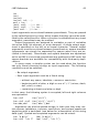
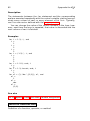
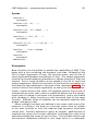
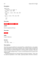
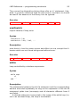
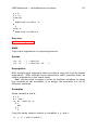
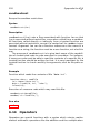
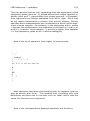
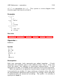
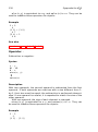
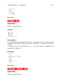
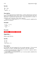
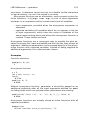
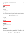
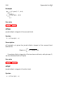
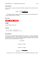
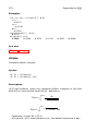
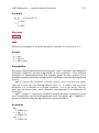
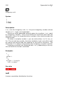
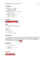
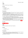
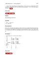
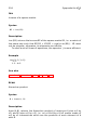
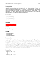
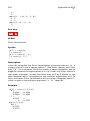
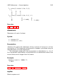
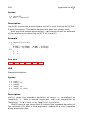
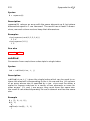
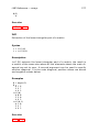
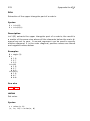
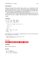
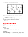
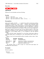
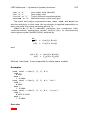
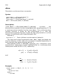
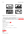
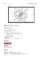
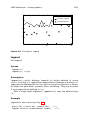
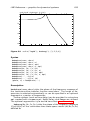
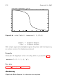
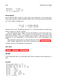
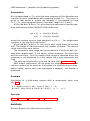
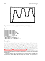
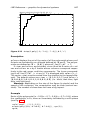
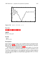
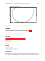
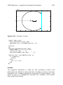
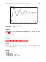
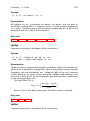
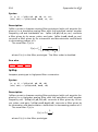
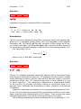
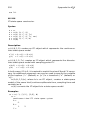
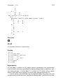
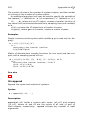
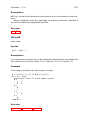
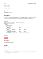
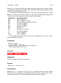
Sysquake for LATEX 454 lsim(..., style, id) (y, t) = lsim(...) Description lsim(numc,denc,u,t) plots the time response of the continuous-time transfer function numd/dend. The input is piece-wise linear; it is defined by points in real vectors t and u, which must have the same length. Input before t(1) and after t(end) is 0. The input used for the simulation is interpolated to have a smooth response. lsim(Ac,Bc,Cc,Dc,u,t) plots the time response of the continuous-time state-space model (Ac,Bc,Cc,Dc) defined as d (t) dt y(t) = Ac (t) + Bc (t) = Cc (t) + Dc (t) where the system input at time sample t(i) is u(i,:)’. For singleinput systems, u can also be a row vector. lsim(Ac,Bc,Cc,Dc,u,t,x0) starts with initial state x0 at time t=0. The length of x0 must match the number of states. The default initial state is the zero vector. Options can be provided in a structure opt created with responseset: ’Range’ The range is a vector of two elements, the start time and the end time. Such an explicit time range is required when the response is not displayed in a plot where the x axis represents the time. ’tOnly’ When opt.tOnly is true, lsim produces output only at the time instants defined in t. The logical value false gives the default interpolated values. The optional arguments style and id have their usual meaning. With output arguments, lsim gives the output and the time as column vectors (or an array for the output of a multiple-output statespace model, where each row represents a sample). No display is produced. Example Response of continuous-time system given by its transfer function with an input defined by linear segments (see Fig. 6.18): t = [0, 10, 20, 30, 50]; u = [1, 1, 0, 1, 1]; lsim(1, [1, 2, 3, 4], u, t, ’b’);