Download SIA-3000 User`s Guide and Reference Manual

Signal Integrity Analyzer 3000
User’s Guide and Reference Manual
200053-06
REV A
This page intentionally left blank.
WAVECREST Corporation continually engages in research related to
product improvement. New material, production methods, and design
refinements are introduced into existing products without notice as a
routine expression of that philosophy. For this reason, any current
WAVECREST product may differ in some respect from its published
description but will always equal or exceed the original design
specifications unless otherwise stated.
Copyright 2005
WAVECREST Corporation
A Technologies Company
7626 Golden Triangle Drive
Eden Prairie, Minnesota 55344
(952) 831-0030
(800) 733-7128
www.wavecrest.com
All Rights Reserved
U.S. Patent Nos. 4,908,784 and 6,185,509, 6,194,925, 6,298,315 B1, 6,356,850
6,393,088, 6,449,570 and R.O.C. Invention Patent No. 146548; other United States
and foreign patents pending.
GigaView, TailFit, OE-2, PM50, AG-100, and SIA-3000 are trademarks of WAVECREST Corporation.
PCI Express is a registered trademark of PCI-SIG in the United States and/or other countries.
InfiniBand is a registered trademark of the InfiniBand Trade Association.
ATTENTION: USE OF THE SOFTWARE IS SUBJECT TO THE WAVECREST SOFTWARE LICENSE TERMS
SET FORTH BELOW. USING THE SOFTWARE INDICATES YOUR ACCEPTANCE OF THESE LICENSE
TERMS. IF YOU DO NOT ACCEPT THESE LICENSE TERMS, YOU MUST RETURN THE SOFTWARE FOR A
FULL REFUND.
WAVECREST SOFTWARE LICENSE TERMS
The following License Terms govern your use of the accompanying Software unless you have a separate written
agreement with Wavecrest.
License Grant. Wavecrest grants you a license to use one copy of the Software. USE means storing, loading, installing,
executing or displaying the Software. You may not modify the Software or disable any licensing or control features of
the Software.
Ownership. The Software is owned and copyrighted by Wavecrest or its third party suppliers. The Software is the
subject of certain patents pending. Your license confers no title or ownership in the Software and is not a sale of any
rights in the Software.
Copies. You may only make copies of the Software for archival purposes or when copying is an essential step in the
authorized Use of the Software. You must reproduce all copyright notices in the original Software on all copies. You
may not copy the Software onto any bulletin board or similar system. You may not make any changes or modifications
to the Software or reverse engineer, decompile, or disassemble the Software.
Transfer. Your license will automatically terminate upon any transfer of the Software. Upon transfer, you must deliver
the Software, including any copies and related documentation, to the transferee. The transferee must accept
these License Terms as a condition to the transfer.
Termination. Wavecrest may terminate your license upon notice for failure to comply with any of these License
Terms. Upon termination, you must immediately destroy the Software, together with all copies, adaptations and
merged portions in any form.
Limited Warranty and Limitation of Liability. Wavecrest SPECIFICALLY DISCLAIMS ALL OTHER
REPRESENTATIONS, CONDITIONS, OR WARRANTIES, EITHER EXPRESS OR IMPLIED, INCLUDING BUT
NOT LIMITED TO ANY IMPLIED WARRANTY OR CONDITION OF MERCHANTABILITY OR FITNESS
FOR A PARTICULAR PURPOSE. ALL OTHER IMPLIED TERMS ARE EXCLUDED. IN NO EVENT WILL
WAVECREST BE LIABLE FOR DIRECT, INDIRECT, SPECIAL, INCIDENTAL, OR CONSEQUENTIAL
DAMAGES ARISING OUT OF THE USE OF OR INABILITY TO USE THE SOFTWARE, WHETHER OR NOT
WAVECREST MAY BE AWARE OF THE POSSIBILITY OF SUCH DAMAGES. IN PARTICULAR,
WAVECREST IS NOT RESPONSIBLE FOR ANY COSTS INCLUDING, BUT NOT LIMITED TO, THOSE
INCURRED AS THE RESULT OF LOST PROFITS OR REVENUE, LOSS OF THE USE OF THE SOFTWARE,
LOSS OF DATA, THE COSTS OF RECOVERING SUCH SOFTWARE OR DATA, OR FOR OTHER SIMILAR
COSTS. IN NO CASE SHALL WAVECREST'S LIABILITY EXCEED THE AMOUNT OF THE LICENSE FEE
PAID BY YOU FOR THE USE OF THE SOFTWARE.
Export Requirements. You may not export or re-export the Software or any copy or adaptation in violation of
any applicable laws or regulations.
U.S. Government Restricted Rights. The Software and documentation have been developed entirely at private
expense and are provided as Commercial Computer Software or restricted computer software.
They are delivered and licensed as commercial computer software as defined in DFARS 252.227-7013 Oct 1988,
DFARS 252.211-7015 May 1991 or DFARS 252.227.7014 Jun 1995, as a commercial item as defined in FAR 2.101 (a),
or as restricted computer software as defined in FAR 52.227-19 Jun 1987 or any equivalent agency regulations or
contract clause, whichever is applicable.
You have only those rights provided for such Software and Documentation by the applicable FAR or DFARS clause or
the Wavecrest standard software agreement for the product.
Table of Contents
Purpose and Organization of this Manual ............................................ xiii
SECTION 1
SIA-3000™ Quick Setup and Measure ................................................. 1
Accessories............................................................................. 1
Quick Setup and Simple Measurement of 10 MHZ Calibration Signal .... 1
Selection of a Measurement Tool ................................................ 3
Turning on the 10 MHZ Square Wave............................................. 4
Taking a Measurement................................................................. 5
SECTION 2
Front and Back Panel Descriptions .................................................... 7
Front Panel Description............................................................. 7
Back Panel Description.............................................................. 11
SECTION 3
Complete Setup of the SIA-3000 ...................................................... 13
Inspection ............................................................................... 13
Connecting Power..................................................................... 14
Connecting a Pointing Device....................................................... 15
Connecting the Keyboard ........................................................... 15
Attaching Peripheral Devices...................................................... 16
Connecting an External Monitor............................................ 16
Connecting a GPIB Cable ..................................................... 16
Connecting to the Network Interface Card ............................. 17
Connecting and Installing a Printer ....................................... 28
SECTION 4
GigiView ™ Software....................................................................... 29
Using GigiView ........................................................................... 30
Getting Started Wizard............................................................... 30
Menu Bar ................................................................................ 31
Tool Pull-down Menu .......................................................... 31
Edit Pull-down Menu ........................................................... 32
Action Pull-down Menu........................................................ 33
Calibration Pull-down Menu ................................................. 33
Macro Pull-down Menu........................................................ 33
Display Pull-down Menu ...................................................... 33
View Pull-down Menu .......................................................... 34
Accessories Pull-down Menu................................................ 34
Help Pull-down Menu.......................................................... 34
Toolbar .................................................................................. 35
Initial Dialog Bar ...................................................................... 36
Dialog Bars ............................................................................. 37
MEASUREMENT TOOLS ...................................................................... 39
Oscilloscope Tool ................................................................... 41
Applications - Overview ....................................................... 41
Oscilloscope Dialog Bars ................................................... 42
Making an Oscilloscope Measurement - Setup Directions ........... 43
Interpreting Oscilloscope Views (Plots)................................. 44
Time View with Eye Mask Enabled ..................................... 44
Summary View.............................................................. 45
Oscilloscope Theory of Operation ........................................ 46
Table of Contents | v
SECTION 4a
CLOCK TOOLS .............................................................................. 47
Clock Analysis Histogram Tool – Applications............................. 49
Making a Clock Analysis Measurement - Setup Directions ........ 50
Interpreting Histogram Tool Views (Plots) ............................ 51
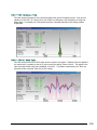
Oscilloscope View .................................................... 51
Histogram View ......................................................... 52
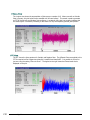
Total Jitter View....................................................... 53
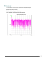
FFT View .................................................................. 54
Clock Analysis theory ...................................................... 55
Histogram Tool – Applications ................................................. 57
Making an Histogram Measurement - Setup Directions ............. 58
Interpreting Histogram Tool Views (Plots) ............................ 59
Accum View .............................................................. 59
Maxi View ................................................................. 60
Bathtub View............................................................ 61
Summary View ........................................................... 62
Histogram Theory ............................................................ 64
Histogram Tool Examples .................................................. 65
Single-Mode Histogram............................................... 66
Bimodal Histogram - Equal Heights ............................... 67
Bimodal Histogram - Unequal Heights............................ 68
High Frequency Modulation Analysis (HFMA) Tool - Applications...... 69
Making an HFMA Measurement - Setup Directions ................... 70
Interpreting HFMA Tool Views (Plots) .................................. 71
1-Sigma View ............................................................ 71
Peak-Peak View.......................................................... 72
FFT N-clock View ....................................................... 73
FFT 1-clock View....................................................... 74
Summary View ........................................................... 75
HFMA Theory .................................................................. 76
Strip Chart Tool................................................................... 77
Making a Strip Chart Measurement - Setup Directions............. 77
Interpreting Strip Chart Tool Views (Plots).......................... 78
Ave/Max/Min View ....................................................... 78
Peak-Peak / 1-Sigma View ............................................. 79
Summary View ........................................................... 79
Strip Chart Theory .......................................................... 80
PLL Analysis Tool.................................................................. 81
Making a PLL Analysis Measurement - Setup Directions............ 82
Interpreting PLL Analysis Tool Views (Plots)......................... 83
1-Sigma Plot ............................................................ 83
PLL Transfer Plot..................................................... 84
Bode Plot ............................................................... 85
Poles and Zero Plot ................................................. 86
Summary Plot........................................................... 87
PLL Analysis Theory ......................................................... 88
vi | Table of Contents
SECTION 4b
OTHER CLOCK TOOLS ......................................................................... 89
Statistics Tool .......................................................................... 90
Low Frequency Modulation Analysis (LFMA) Tool .............................. 91
Making a LFMA Measurement - Setup Directions .......................... 92
Interpreting LFMA Tool Views (Plots) ....................................... 92
Time View ...................................................................... 92
FFT 1-clock View ........................................................... 93
Summary View ................................................................ 94
LFMA Theory........................................................................ 95
Phase Noise Tool ....................................................................... 97
Making a Phase Noise Measurement - Setup Directions ................. 97
Interpreting Phase Noise Tool Views (Plots) .............................. 98
FFT View ....................................................................... 98
Summary View ................................................................ 99
Phase Noise Theory ............................................................. 100
Locktime Tool - Applications........................................................ 101
Making a Locktime Measurement - Setup Directions .................... 102
Interpreting Locktime Tool Views (Plots).................................. 103
Time View ..................................................................... 103
FFT View ...................................................................... 104
1-Sigma View ................................................................ 105
Peak-Peak View ............................................................. 106
Summary View ............................................................... 107
Locktime Theory .................................................................. 108
Cycle-to-Cycle Tool .................................................................. 111
Making a Cycle-to-Cycle Measurement - Setup Directions ............ 111
Interpreting Cycle-to-Cycle Tool Views (Plots) ......................... 112
Norm Adjacent View ...................................................... 112
Acum Cycle-to-Cycle View............................................... 113
Maxi Cycle-to-Cycle View ................................................ 114
Bathtub ...................................................................... 115
Summary View ............................................................... 116
Cycle-to-Cycle Theory.......................................................... 117
DRCG Tool - Applications............................................................ 119
Making a DRCG Measurement - Setup Directions......................... 120
Interpreting DRCG Tool Views (Plots)...................................... 121
Jitter Plot View ........................................................... 121
DRCG Summary View....................................................... 122
DRCG Theory ...................................................................... 123
Spread Spectrum clock Tool ...................................................... 125
Making a Spread Spectrum Measurement - Setup Directions......... 125
Interpreting Spread Spectrum Tool Views (Plots) ...................... 126
Histogram View ............................................................. 126
1-Sigma View ................................................................ 127
Spread Spectrum Summary View....................................... 128
Spread Spectrum Clock Theory ............................................. 129
Table of Contents | vvii
SECTION 4c
DATA TOOLS.............................................................................. 131
Known Pattern with Marker Tool - Applications ........................... 132
Making a KPWM Measurement - Setup Directions .................... 135
Interpreting Known Pattern with Marker Tool Views (Plots)..... 135
DCD + ISI Histogram View ........................................... 136
DCD + ISI vs. Edge View ............................................. 137
1-Sigma View ............................................................ 138
FFT View .................................................................. 139
Bathtub View............................................................ 140
UI Distribution View ................................................... 141
Summary View ........................................................... 142
KPWM Theory .................................................................. 143
Random Data with Bit Clock Tool .............................................. 145
Making a RDBC Measurement - Setup Directions..................... 146
Interpreting Random Data with Bit Clock Tool Views (Plots)..... 147
Histogram View ......................................................... 147
Probability Histogram View ......................................... 148
Bathtub View............................................................ 149
Summary View ........................................................... 150
RDBC Theory .................................................................. 151
Random Data No Marker Tool ................................................... 155
Making a RDNM Measurement - Setup Directions .................... 156
Interpreting RDNM Tool Views (Plots).................................. 157
DCD + ISI View ......................................................... 157
1-Sigma View ............................................................ 158
FFT View .................................................................. 159
Bathtub View............................................................ 160
Summary View ........................................................... 161
RDNM Theory .................................................................. 162
Known Pattern with Bit Clock and Marker Tool ........................... 163
Making a KPBC Measurement - Setup Directions ..................... 163
Interpreting KPBC Tool Views (Plots) .................................. 165
Total Histogram View ................................................. 165
DCD + ISI Histogram View ........................................... 166
DCD + ISI vs. Span View ............................................. 167
1-Sigma View ............................................................ 168
FFT View .................................................................. 169
Bathtub View............................................................ 170
Summary View ........................................................... 171
KPBC Theory .................................................................. 172
viii | Table of Contents
SECTION 4d
DATA STANDARDS TOOLS ..................................................................... 175
PCI Express 1.1 Hardware Clock Recovery (CR) Tool ......................... 175
Making a PCIX Hardware CR Measurement - Setup Directions .......... 176
Interpreting PCIX Hardware CR Views (Plots) .............................. 177
Oscilloscope View .......................................................... 177
Transition Eye View .......................................................... 178
De-emph Eye View ............................................................ 178
Total Jitter Histogram View .............................................. 179
Bathtub View.................................................................. 179
Summary View ................................................................. 179
PCI Express 1.1 Software Clock Recovery (CR) Tool ....................... 181
Making a PCIX Software CR Measurement - Setup Directions ........ 181
Interpreting PCIX Software CR Views (Plots) ............................ 183
Oscilloscope View ........................................................ 183
Trans Eye View.............................................................. 184
De-emph Eye View .......................................................... 184
Median to Maximum histogram View.................................... 184
DCD + ISI Histogram View............................................... 185
DCD + ISI vs. Span Histogram View................................... 185
1-Sigma vs. Span View .................................................... 185
FFT View ...................................................................... 186
Bathtub Curve View....................................................... 186
PCI Express 1.1 Clock Analysis Tool ............................................ 187
PCI Express 1.0a Tool ............................................................... 189
Making a PCI Express 1.0a Measurement - Setup Directions......... 189
Interpreting PCI Express Views (Plots) .................................... 190
Oscilloscope View ........................................................ 180
Trans Eye View.............................................................. 191
De-emphasized View ..................................................................................192
Total Histogram View ..................................................... 193
Bathtub Curve View....................................................... 193
Summary View ............................................................... 194
PCI Express Theory.............................................................. 195
Fibre Channel Compliance Tool .................................................... 197
Making a Fibre Channel Measurement - Setup Directions ............. 198
Interpreting Fibre Channel Tool Views (Plots) .......................... 199
Oscilloscope View ........................................................ 199
DCD + ISI Histogram View............................................... 200
DCD + ISI vs. Span View ................................................. 200
1-Sigma View ................................................................ 200
FFT View ...................................................................... 201
Bathtub View................................................................ 201
Summary View ............................................................... 201
Fibre Channel Theory ........................................................... 202
Table of Contents | ix
Serial ATA II Hardware Clock Recovery (CR) Tool ............................ 203
Making a SATA II Hardware CR Measurement – Setup Directions .... 204
Interpreting SATA II Hardware CR Tool Views (Plots) .................. 205
Histogram View ............................................................. 205
Eye Diagram View .......................................................... 205
Bathtub Curve View....................................................... 206
Summary View ............................................................... 206
Serial ATA II Software Clock Recovery (CR) Gen1x-Gen2x Tool........... 207
Making a SATA II Software CR Measurement – Setup Directions .... 207
Interpreting SATA II Software CR Tool Views (Plots) .................. 208
Oscilloscope View ........................................................ 208
DCD + ISI Histogram View............................................... 209
DCD + ISI vs. Span View ................................................. 209
1-Sigma View ................................................................ 210
FFT View ...................................................................... 210
Bathtub Curve View....................................................... 211
Summary View ............................................................... 211
Serial ATA 1.0 Tool .................................................................. 213
Making a Serial ATA Measurement - Setup Directions .................. 213
Interpreting Serial ATA Tool Views (Plots) ............................... 213
Jitter vs. Span View ...................................................... 214
Histograms View ........................................................... 214
Summary View ............................................................... 214
Serial ATA 1.0 Theory ......................................................... 215
InfiniBand Tool ......................................................................... 217
Making an InfiniBand Measurement - Setup Directions.................. 214
Interpreting InfiniBand Tool Views (Plots) ................................ 218
Histogram View ............................................................. 218
Eye Diagram View .......................................................... 218
Bathtub ...................................................................... 219
Summary View ............................................................... 219
x
| Table of Contents
SECTION 4e
SECTION 4f
SECTION 4g
CHANNEL-To-CHANNEL TOOLS.............................................................. 221
Propagation Delay and Skew Tool ................................................. 221
Making a Propagation Delay Measurement - Setup Directions ....... 221
Interpreting Propagation Delay and Skew Tool Views (Plots) ....... 222
Accumulated Histogram View........................................... 222
Maxi Histogram View ...................................................... 223
Bathtub Histogram View ................................................. 224
Summary View ............................................................... 225
Propagation Delay and Skew Theory ........................................ 226
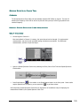
Data Bus Tool .......................................................................... 227
Making a Data Bus Measurement - Setup Directions .................... 228
Interpreting Data Bus Views (Plots) ........................................ 229
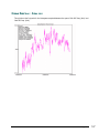
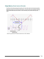
Data Histogram View ...................................................... 229
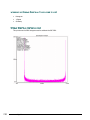
Data Bathtub View......................................................... 230
Clock Histogram View .................................................... 231
Clock Bathtub View....................................................... 232
Data Bus Summary View .................................................. 233
Data Bus Theory.................................................................. 234
Locktime Tool........................................................................... 235
Making a Locktime Measurement - Setup Directions .................... 235
Interpreting Locktime Views (Plots)......................................... 236
Time View ..................................................................... 236
FFT View ...................................................................... 237
1-Sigma View ................................................................ 238
Pk-Pk View ................................................................... 239
Summary View ............................................................... 240
Locktime Theory .................................................................. 241
Help TOOLS .................................................................................... 243
Other Tools ................................................................................... 243
Jitter Generator ...................................................................... 247
Switch Matrix ........................................................................... 249
Arm Generator ......................................................................... 253
Optical Interface ...................................................................... 257
Pattern Marker (PM50) .............................................................. 259
Folded Eye Diagram ................................................................... 265
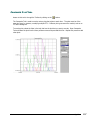
Composite Plot Tool ........................................................................ 267
APPENDIX A - Macro Overview ................................................................................ 271
APPENDIX B - Tailfit™ Theory................................................................................. 281
APPENDIX C - Calibration ...................................................................................... 283
APPENDIX D - Specifications and Maintenance............................................................. 289
APPENDIX E - Clock Recovery Option....................................................................... 293
APPENDIX F - Remote GigaView Installation ................................................................ 295
GLOSSARY of TERMS ............................................................................................ 299
Table of Contents | xi
This page intentionally left blank.
x
| Table of Contents
Purpose and Organization of this Manual
The purpose of this manual is to provide the user with a quick overview of the Signal Integrity Analyzer
3000™ (SIA-3000) and GigiView ™ software.
Parts of this manual have been compiled from the online Help system included with the GigiView software. Some areas
will appear different due to the presentation and layout format of the Help system versus the hard copy manual format. It
is recommended that this manual be used as a supplement to the online Help system and to the Quick Reference
Guides included with the SIA-3000. Parts of the manual may differ from the software appearance due to changes
and modifications of the software.
In general, this manual is an overview of the functions and operation of the SIA-3000 and GigiView software. It is
assumed that the user has some familiarity with test equipment such as signal generators and oscilloscopes as well as the
terminology involved with their usage.
The manual has been organized as follows:
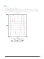
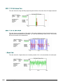
Section 1 - SIA-3000 Quick Setup and Measure
This section helps the user to quickly set up the instrument and take a simple Histogram measurement using the 10MHz
Calibration OUT signal.
Section 2 – Front and Back Panel Descriptions
This section describes the front and back panel operation of the instrument.
Section 3 – Complete Setup of the SIA-3000
This section shows the user how to inspect and fully set up the SIA-3000 including accessories and peripherals.
Section 4 – GigiView Software
This section describes the basic controls and features of GigiView including the setup of all measurement tools.
Appendix A contains an overview of GigiView Macro features including detailed examples of each Macro command.
Appendix B contains a detailed explanation of TailFit™ theory.
Appendix C
describes the calibration options of the SIA-3000.
Appendix D
lists the SIA-3000 performance and maintenance specifications.
Appendix E describes the Clock Recovery option of the SIA-3000.
Appendix F describes the installation of Remote GigiView.
Glossary contains detailed definitions of menu selections, functions, dialog bar selections and jitter related terminology.
©WAVECREST Corporation 2005
xiii
This page intentionally left blank.
xiv
©WAVECREST Corporation 2005
SECTION 1– SIA-3000™ Quick Setup and Measure
This section helps the user to quickly set up the WAVECREST Signal Integrity Analyzer 3000 (SIA3000) and take a simple measurement using the 10MHz Calibration OUT signal. In addition, this section
will assist the user in calibrating the SIA-3000. The accessories included with the unit are listed below.
Accessories
Keyboard
Pointing device (mouse)
Power cord
Two (2) 50Ω coaxial cables with SMA connectors
SIA3000 User’s Guide and Reference Manual
SIA3000 GPIB Programming Guide
Two (2) SMA Quick Connect adapters for calibration (minimum 500 uses)
Quick Setup and Simple Measurement of 10 MHZ Calibration Signal
This section will show the user how to:
•
•
•
Attach the included keyboard, mouse and power cord to the SIA-3000
Attach a coax cable to an input channel and the Calibration OUT signal
Open a GigaView measurement tool
The following steps will show the user how to attach the keyboard, mouse, coax cable and power cord.
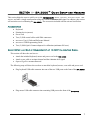
Plug keyboard USB cable connector into one of the two USB ports on the front of the SIA-3000.
Plug mouse USB cable connector into remaining USB port on the front of the SIA-3000.
©WAVECREST Corporation 2005
Section 1 - Quick Setup
1
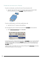
Attach coax cable to the (Channel 1) IN 1 connector. Ensure there is a tight connection.
Attach other end of coax cable to the Calibration OUT connector. Ensure there is a tight
Connection (~7-9 in/lbs).
Plug female end of power cord into power cord connection on back of unit.
Plug male end of power cord into an appropriately grounded 115 VAC source.
Turn on power by pushing the power button at the bottom right-hand corner of the front panel.
After a few minutes, the opening view of GigaView’s work area will be displayed.
2
Section 1 - Quick Setup
©WAVECREST Corporation 2005
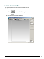
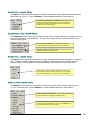
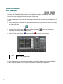
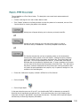
Selecting a Measurement Tool
The following steps will select the Histogram Tool using the Dialog Bar.
From the opening view:
Click on
to access the Clock Tools Dialog Bar.
Click on
to open the Histogram Tool.
©WAVECREST Corporation 2005
Section 1 - Quick Setup
3
Turning on the 10MHz Square Wave
The following steps will show the user how to select and enable the Calibration Signal Output signal.
Click on the Calibration pull-down menu of the main Menu Bar.
Select the 10MHz option in the pull-down menu of the dialog box.
The Calibration OUT connection will now be outputting a 10MHz square wave.
4
Section 1 - Quick Setup
©WAVECREST Corporation 2005
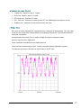
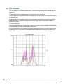
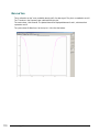
Taking a Measurement
Click the
button (Single/Stop) on the tool bar to view a histogram of the 10MHz square wave.
Note: When a tool is first opened, a pulsefind is automatically performed when a measurement is
taken. Should any parameter setting or input signal changes occur, a pulsefind should be
performed prior to taking another measurement.
If an error is received, ensure all connectors are tight and re-activate the 10MHz calibration signal as
described in the previous instructions.
Redo a Pulsefind (
) and then take another Single measurement (
©WAVECREST Corporation 2005
).
Section 1 - Quick Setup
5
This page intentionally left blank.
6
Section 1 - Quick Setup
©WAVECREST Corporation 2005
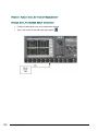
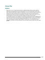
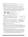
SECTION 2 - Front and Back Panel Descriptions
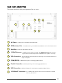
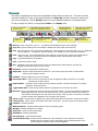
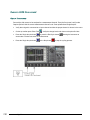
FRONT PANEL DESCRIPTION
This section describes the front panel operation of the SIA-3000.
4
7
PULSE
FIND
1
3
8
5
6
2
10
9
11
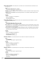
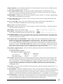
Figure 2.1 - SIA-3000 Front panel
1
Front Panel Display - Flat LCD color display for viewing GigaView tools/measurements.
2
Channel Card Inputs - Measurement channels: up to 10 single-ended or differential input channel cards
can be configured.
3
Tool/Field Selection Buttons - Buttons correspond to adjacent fields/buttons on LCD. Pressing
button activates corresponding field/button.
©WAVECREST Corporation 2005
Section 2 - Front and Back Panel Description
7
4
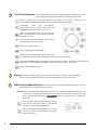
Tool Function Buttons - Used for displaying tool selections, starting/stopping measurements, clearing
current display measurements, disabling all tools and enabling markers.
Pressing on this button will display GigaView tool buttons on the display. Pressing on the
corresponding Tool/Field Selection button will activate the desired measurement tool.
Continuously
acquire
new
measurements.
Measurements will be acquired until either the
Single/Stop button is pressed or an error occurs.
Acquires a single measurement. Also used to stop a
series of measurements from being taken after the
Run button is pressed.
Dial
- Used to increment/decrement values of active field or
scroll through choices of active field.
Clears active window of data.
Stops all running tools simultaneously.
Performs a pulse find. Performs a peak-to-peak voltage
measurement and sets the voltage threshold to be used for timing measurements.
Scrolls through Marker options by displaying current selection on window. Selections include: Horizontal
markers only, Vertical markers only, both Horizontal and Vertical markers or no markers.
Enables displayed Marker option.
5
Keypad - Keypad is used for entering values into active fields. The “<” button is used as a backspace
button to erase the highlighted number or the number immediately to the left of the cursor.
6
USB Connector/Macro Buttons - USB connectors are for keyboard and pointing device accessories.
Macro buttons are for recording and playing macros.
- For connecting included USB accessories or any other hot swappable peripheral devices
to instrument. An additional USB connection is located on the back panel. If connecting a USB
device other than those provided by WAVECREST, make sure the device driver is available for
installation.
USB Connectors
Press on the Rec. button to begin recording a series of
steps from the front panel, mouse or keyboard that
can then be replayed using the Play button.
Press on the Play button to playback a series of steps
that were previously recorded from the front panel,
mouse or keyboard.
8
Section 2 - Front and Back Panel Description
©WAVECREST Corporation 2005
7
File Output/Input Function Buttons - Used for storing or loading measurement data, tool
configurations and data patterns.
Press on the Print button to print current tool
window plot.
Press on the Load button to load previously
saved plots, configurations or settings.
Press on the Save button to save plots,
configurations or settings.
Press on the Local button to regain front
panel system control from GPIB instrument
control.
Press on the Help button to activate the
online Help system.
8
Scaling and Position Control Dials - Adjusts x- and y-axis viewing position and scaling.
©WAVECREST Corporation 2005
Section 2 - Front and Back Panel Description
9
9
Menu Navigation and Display Control Buttons - Activates pull-down menus of
GigaView software and allows navigation/selection of menu choices and online Help system. Display
control buttons scroll through open tools, add or close tools or clear all tools.
Press on the Menu button to activate the
pull-down menus of the GigaView Menu
bar.
Press on the Tab button to jump from
field to field in the active GigaView tool.
Arrow buttons - Press on an arrow to move the
highlighted cursor area up or down the
active pull-down menu or to the adjacent
pull-down menu.
Pressing on Clear button clears active tool
of any measurements or plots.
Pressing the Next button will switch to
the next tool or view.
Pressing on the
active tool
Close
button closes the
Pressing the Add View button will open a
new window of the active tool.
10
10
Power Button - Turns on/off SIA-3000.
11
Calibration OUT - Supplies calibration and reference signals for calibrating the SIA-3000.
Section 2 - Front and Back Panel Description
©WAVECREST Corporation 2005
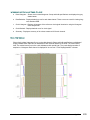
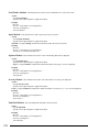
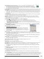
BACK PANEL DESCRIPTION
This section describes the back panel operation of the SIA-3000.
2
3
5
6
8
9
7
4
1
1
AC Power - Where power cord attaches to the SIA-3000.
2
GPIB Interface Port - The GPIB interface provides IEEE-488 standard bus services for the SIA-3000.
3
Arm/Gate - Feature not implemented at this time.
4
10 MHz Reference - A 10MHz reference signal is provided. The 10MHz Reference In port is used as a
bypass if the user already incorporates a 10MHz Reference signal for a test setup
5
VGA Connection - The SIA-3000 includes the option of connecting a VGA-compatible monitor for a
larger viewing area.
6
COM2 (RS232) - Additional serial port for connecting peripheral devices.
7
Parallel Connection - Additional parallel port for connecting peripheral devices.
8
USB Connection - Additional USB port for connecting hot-swappable peripheral devices.
9
10/100BaseT Connection - A 10/100BaseT NIC card for LAN or network connections is included
with every SIA-3000.
©WAVECREST Corporation 2005
Section 2 - Front and Back Panel Description
11
This page intentionally left blank.
12
Section 2 - Front and Back Panel Description
©WAVECREST Corporation 2005
SECTION 3 – Complete Setup of the SIA-3000
This section shows you how to inspect and fully set up the SIA-3000 including the attachment
of accessories and peripheral devices. The following areas are covered in this section:
•
Inspection
•
Connecting power
•
Connecting included accessories
•
Connecting peripheral devices
•
Verify instrument is taking measurements
Inspection
Inspect the shipping box for damage.
If the box is damaged, retain it until the contents and instrument have been checked for
damage and proper operation.
Check for accessories.
Keyboard
Pointing device (mouse)
Power cord
Two (2) matched 50Ω coaxial cables with SMA connectors
Two (2) SMA Quick Connect calibration adapters (Minimum 500 uses)
SIA-3000 User’s Guide and Reference Manual and 3-ring binder
SIA-3000 GPIB Programming Guide and 3-ring binder
SIA-3000 LabVIEW Programming Guide and software drivers CDROM
GigaView Quick Reference Guides and 3-ring binder
If the contents are incomplete or damaged, contact WAVECREST Corporation Customer
Service: 1-800-733-7128
Inspect the instrument.
If there is mechanical/physical damage, or if the instrument does not power up or boot up
properly, notify WAVECREST Corporation.
If the shipping box is damaged, or the cushioning materials show signs of stress, notify
the shipping carrier as well as the WAVECREST Corporation office. Keep the shipping
materials for the carrier’s inspection. WAVECREST Corporation will arrange for repair
or replacement at their option.
©WAVECREST Corporation 2005
Section 3 - Complete Setup of the SIA-3000
13
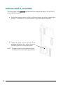
Connecting Power to the SIA-3000
The power supply of the SIA-3000 operates with a line voltage in the range of 100 to 230VAC
at 50-60 HZ line frequency.
Position the instrument where it will have sufficient clearance for airflow around the back
and sides. A minimum of 2-3 inches clearance is required for the back and sides.
Connect the power cord to the rear of the
instrument and then to an ac outlet. Ensure the
outlet has a protective earth ground contact.
NOTE: The power supply fan will automatically turn
on when power is connected to the instrument.
14
Section 3 - Complete Setup of the SIA-3000
©WAVECREST Corporation 2005
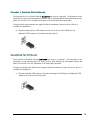
Connect a Pointing Device/Mouse
The pointing device is included with the SIA-3000 but using it is optional. All operations of the
instrument, except for entering alpha file names, can be done through the front panel buttons and
knobs. See Section 2 for a complete description of front and back panel operations.
If using a mouse other than the one supplied with the instrument, ensure the device driver is
available for installation.
Plug the pointing device USB connector into one of the two front USB ports (an
additional USB connector is located on the back panel).
Connecting the Keyboard
The keyboard is included with the SIA-3000 but using it is optional. All operations of the
instrument, except entering alpha file names, can be done through the front panel buttons and
knobs. See Section 2 for an explanation of all front panel operations.
If using a keyboard other than the one supplied with the instrument, ensure the device driver is
available for installation.
Plug the keyboard USB connector into the remaining front USB port (an additional USB
connector is located on the back panel).
©WAVECREST Corporation 2005
Section 3 - Complete Setup of the SIA-3000
15
ATTACHING PERIPHERAL DEVICES TO THE SIA-3000
Connecting an External Monitor
The SIA-3000 has the option of connecting a VGA-compatible monitor for a larger viewing area.
Ensure the device driver is available for installation.
Power down the SIA-3000.
Attach the monitor cable to the VGA connection on the back panel of the SIA-3000.
Tighten the retaining screws.
Power up the monitor before powering up the SIA-3000.
Power up the SIA-3000.
* If the system requires a new monitor driver, select the files from the c:\win98 directory (see
procedure below)
Select ‘Next’ to verify the installation procedure.
Select ‘Search for the best driver for your device.’
Specify a location: c:\win98
Windows will detect the driver
Select ‘Next’ to install the driver
Select ‘Finish’
Connecting a GPIB Cable to the SIA-3000
Attach the GPIB cable connector to the GPIB (IEEE.488) interface card connector on the
back panel of the SIA-3000. Tighten the thumbscrews.
16
Section 3 - Complete Setup of the SIA-3000
©WAVECREST Corporation 2005
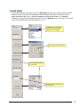
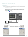
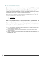
Connecting to the Network Interface Card (NIC)
A 10/100BaseT NIC card is included with every SIA-3000. Consult with your company’s
information systems personnel to ensure your LAN system is compatible with the SIA-3000
network card and to establish a local network connection.
Plug the RJ45 cable connector into the RJ45 connection on the back panel.
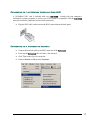
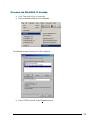
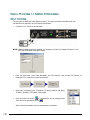
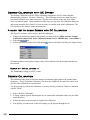
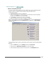
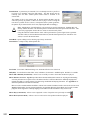
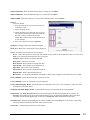
Connecting to a Microsoft® Network
Connect the network cable to the RJ45 connector of the SIA-3000.
Power up the SIA-3000 (this will take a few minutes).
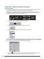
Click Tool on the GigaView menu bar.
Point to Network and then select Properties.
©WAVECREST Corporation 2005
Section 3 - Complete Setup of the SIA-3000
17
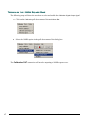
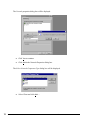
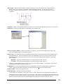
The Network properties dialog box will be displayed.
Click Yes to continue.
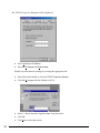
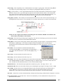
Click Add in the Network Properties dialog box.
The Select Network Component Type dialog box will be displayed.
Select Client and click Add….
18
Section 3 - Complete Setup of the SIA-3000
©WAVECREST Corporation 2005
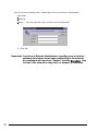
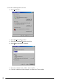
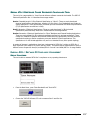
The Select Network Client dialog box will be displayed.
Select ‘Microsoft’ for the Manufacturers.
Select ‘Client for Microsoft Networks’ for the Network Clients.
Click OK.
The complete Network properties dialog box will be displayed.
Click OK on the Network dialog window
Click Yes to restart the system.
©WAVECREST Corporation 2005
Section 3 - Complete Setup of the SIA-3000
19
Once the system is running, enter: (Obtain these from your Network Administrator)
User name:
Password:
Domain:
(once you enter this value it will be stored automatically)
Click OK
Important: Consult your Network Administrator regarding virus protection
software and security issues before connecting to the network.
Virus software will need to be “Pushed” onto the SIA-3000. Also
find out if the network is using static or dynamic IP addresses.
20
Section 3 - Complete Setup of the SIA-3000
©WAVECREST Corporation 2005
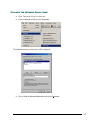
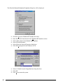
Changing the Network Domain Name
Click Tool on the GigaView menu bar.
Point to Network and then select Properties.
The Network properties dialog box will be displayed.
Select Client for Microsoft Networks and select Properties.
©WAVECREST Corporation 2005
Section 3 - Complete Setup of the SIA-3000
21
The Client for Microsoft Networks Properties dialog box will be displayed.
Check the Log on to Windows NT domain check box.
Enter the network domain name in the Windows NT domain: text box.
Select either option for the Network logon options.
Select OK when finished.
Select OK on the Network Properties dialog box.
Click OK if prompted for the Windows 98 CD.
Select C:\Win98 from the Copy files from: drop down box.
Click OK
Click Yes to restart the system.
22
Section 3 - Complete Setup of the SIA-3000
©WAVECREST Corporation 2005
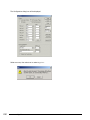
Changing the SIA-3000 IP Address
Click Tool on the GigaView menu bar.
Point to Network and then select Properties.
The Network properties dialog box will be displayed.
Select TCP/IP and click on the Properties button.
©WAVECREST Corporation 2005
Section 3 - Complete Setup of the SIA-3000
23
The TCP/IP Properties dialog box will be displayed.
Select Specify an IP address.
Enter the IP Address and Subnet Mask.
Modify any other network settings by selecting the appropriate tab.
Select OK when finished to close the TCP/IP Properties Window.
Click OK if prompted for the Windows 98 CD.
Select C:\Win98 from the Copy files from: drop down box.
Click OK.
Click Yes to restart the system.
24
Section 3 - Complete Setup of the SIA-3000
©WAVECREST Corporation 2005
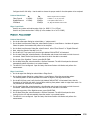
Performing the Scandisk and Defragmentation of the Local Disk
Select Tool on the GigaView menu bar
Point to Network and then select Share Drive on Network…
The local drive properties dialog box will be displayed.
Select the Tools tab.
©WAVECREST Corporation 2005
Section 3 - Complete Setup of the SIA-3000
25
Use the Error-checking status tool first.
Select Check Now…
Select Standard for Type of test.
Select the Automatically fix errors check box
Select Start to perform the Scandisk
Close the Scandisk results window when complete
Close the Scandisk tool when complete to return to the Tools window
26
Section 3 - Complete Setup of the SIA-3000
©WAVECREST Corporation 2005
Next, use the Defragmentation status tool.
Select Defragment Now…
The Defragmenting Drive C: popup box will be displayed.
Select Yes to exit Disk Defragmenter when defragmentation is done.
Select OK to exit the Tools window.
The local disk has now been defragmented and scanned for errors.
©WAVECREST Corporation 2005
Section 3 - Complete Setup of the SIA-3000
27
Connecting and Installing a Printer
If you have a serial printer, you will need a 9-pin to 25-pin serial printer cable.
Attach the 9-pin small “D” connector to the printer output connector labeled COM2
(RS232) on the back panel of the SIA-3000. Tighten the thumbscrews.
If you have a parallel printer, you will need a parallel printer cable.
Attach the 25-pin “D” connector to the parallel port.
Once the appropriate printer cable has been attached and the SIA-3000 has been turned on,
Select Tool/Print Setup/Add Printer from the Menu Bar.
Locate the target printer, whether hooked up locally to the SIA-3000 or over a network, through
the dialog boxes that appear following the Add Printer selection. Make sure the printer driver is
available on a floppy disk or at a network location accessible by you if it is not included on the
SIA-3000 printer list.
Additional printers can be added, removed or configured through the Tool/Print Setup selection by
following the dialog boxes and screen prompts.
28
Section 3 - Complete Setup of the SIA-3000
©WAVECREST Corporation 2005
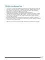
SECTION 4 – GigaView Software
Introducing GigaView Software
WAVECREST’s GigaView software is the latest software package to address the growing needs of the
electronics industry for analyzing Signal Integrity. Jitter is a major cause of data signal fidelity loss.
GigaView software provides the tools necessary to quantify and isolate these and many more timing
anomalies.
GigaView software provides one of the most comprehensive jitter analysis software packages on the market
today. The Windows-based GUI, Measurement Wizard and online help will enable new users to confidently
acquire useful data in seconds. Even inexperienced users will be capable of making measurements of
accumulated jitter, low and high frequency modulation and frequency locktime enabling them to characterize
and fully understand the performance of their clock signal. Furthermore, the addition of macros allows users
to perform routine tasks at the click of a button.
GigaView may be used as a jitter analysis tool for a variety of data communication protocols including
Fibre Channel and Gigabit Ethernet. GigaView is a comprehensive data analysis package that includes
patented algorithms capable of separating total jitter (TJ) into its deterministic jitter (DJ) and random
jitter (RJ) components and the capability to predict the long-term reliability of systems and components
in seconds.
©WAVECREST Corporation 2005
Section 4 - GigaView
29
Using GigaView
Introduction
This section introduces a new user to the basic controls and features of GigaView software. Refer to the
Help files provided in the GigaView software for more detailed information on the functions and features.
Other Quick Reference Guides describe each tool in detail, including setup, theory of operation and making
measurements.
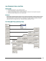
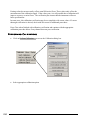
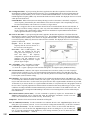
Opening GigaView
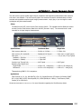
Once GigaView is running on the SIA-3000, the screen will be displayed. Access to GigaView tools is
through the Dialog bar at the right by either clicking on the buttons using a pointing device or pressing the
associated button on the front panel. Specific tools (Histogram, High Frequency Modulation, etc.) are
described in their respective Tool Overview sections in the online help system or in this User's Guide.
Title Bar - Contains the
name of the application
and tool.
Menu Bar - Provides pulldown menus for the many
features in GigaView.
Work Area - Where
active and/or open
tools are displayed.
Toolbar - provides onebutton activation of
common application
features.
Dialog Bar - Contains
tool-specific parameter
options of active window.
Status Bar - Displays status messages, cursor position and tool status.
• “Run“ will appear if “Run“ was pressed in the active window.
• A black bar appears when the unit is performing/computing a measurement.
• A timer displays the elapsed time of the test.
• Cursor coordinates for the active window are displayed when using a pointing device.
30
Section 4 - GigaView
©WAVECREST Corporation 2005
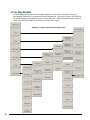
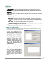
MENU BAR
The Menu Bar is displayed across the top of the application window below the Title Bar. The Menu Bar
provides pull-down menus for accessing the many features in GigaView.
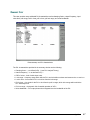
Tool Pull-down Menu
The Tool pull-down menu lists options for opening new or previously saved tool configurations, printing the
displayed window, connecting to a local area network, recalling the four most recent tools used and closing
GigaView. See the Glossary section for a detailed explanation of each selection.
New, Open, Close, Save and Save As - Presents options for
opening, closing or saving a new or previously saved GigaView tool.
Print, Print Preview and Printer Setup - Presents options for
printing, choosing and setting up a printer as well as previewing the
active tool view as it would appear when printed.
Network - Click on this selection to configure the network properties.
Provides access to tools and parameters providing/regulating network
access.
1, 2, 3, 4 List - This area displays the last four tools used. Click on
the number/name that corresponds with the tool to re-open.
Shutdown - Click on this command to end your GigaView session and
shut down the instrument.
©WAVECREST Corporation 2005
Section 4 - GigaView
31
Edit Pull-down Menu
The Edit pull-down menu lists options for editing displayed data as well as customizing display/window
characteristics.
Copy, Clear and Annotation – Copy or clear the currently displayed
data. Annotate the Summary view.
Display Settings – This popup dialog box allows access to display
characteristics of the waveform, text and GUI.
GPIB Configuration – This popup dialog box gives the user easy
access to GPIB addresses and target devices.
Global Tool Settings – This popup dialog box allows access to settings
that affect all tool applications.
CR Configuration – User-configurable settings for the Clock Recover
option.
Optical Configuration – User-configurable Optical device
settings.
32
Section 4 - GigaView
©WAVECREST Corporation 2005
Action Pull-down Menu
The Action pull-down menu lists commands for taking measurements, remote calibration and accessing the
Macro feature of GigaView. See the Glossary for a more detailed explanation of each selection.
Run, Disable All, Single/Stop and Pulsefind - These options are
for taking multiple/single measurements, as well as stopping all
measurements, finding peak voltages and determining threshold
voltages based on current settings.
Calibration Pull-down Menu
The Calibration pull-down menu lists commands for determining if system calibrations are necessary as well
as providing methods for those calibrations. This menu also provides access for selecting calibration and
reference output signals.
Verify and Perform Calibration... - Determines if the SIA-3000
requires calibration and step-by-step instructions for calibration.
Calibration and Reference Signal Output - Provides selections for
calibration and reference signal outputs.
Macro Pull-down Menu
The Macro pull-down menu lists commands for scripting and automating activities performed on a repetitive
basis. The Macro interface is based on Microsoft's VBScript language that includes the ability to control
program execution using conditional and looping statements. See Appendix B or online Help Topics.
Macros can be recorded, modified or written from scratch. The
Macro interface can also be used to access GigaView functionality
from an external application. See Appendix A - Macro Overview.
Display Pull-down Menu
The Display pull-down menu lists commands for configuring the Main Window features, Work Area and
GigaView tool display area. See the Glossary for a more detailed explanation of each selection.
Toolbar, Status Bar and Dialog Bar - A check mark appears next to
the menu item when it is displayed in the Main Window.
This area lists selections for customizing a tool’s display area to aid in
the presentation and interpretation of data. See the Glossary for a
more detailed explanation of each selection.
©WAVECREST Corporation 2005
Section 4 - GigaView
33
View Pull-down Menu
The View pull-down menu lists options for adding a new window with the same contents as the active
window, determining the order and placement of GigaView tools in the Work Area as well as scrolling
between tools. Active tools are displayed at the bottom of the menu and are activated when checked.
See the Glossary for a more detailed explanation of each selection.
Add - Adds a new window with the same contents as the active
window. User can then change the view; a tool typically has different
views associated with it.
Cascade and Tile - Determines the order and placement of
GigaView tools in the Work Area.
Next and Previous - Used for scrolling between active tools.
Composite Plot - Used to overlay various plots which relate to each
other. The plots must be of the same plot type.
This area lists all open/active tools.
Accessories Pull-down Menu
The Accessories pull-down menu lists additional system features.
This area lists resident features of the operating system.
Help Pull-down Menu
The Help pull-down menu provides access to the online help system, version number and technical support
phone number.
Clicking on Help Topics... opens the GigaView online help system.
Wizard, Plot Interpretor and Online Documentation - Clicking on
these selections accesses additional setup and information tools.
Clicking on this selection displays the version number of GigaView as
well as WAVECREST Corporation’s technical support number.
34
Section 4 - GigaView
©WAVECREST Corporation 2005
TOOLBAR
The toolbar is displayed across the top of the application window below the menu bar. The toolbar provides
one-button activation for many of the selections listed in the Menu Bar pull-down menus such as New, Open,
Save, Run and Single/Stop. See the Glossary section for a more detailed explanation of individual buttons.
To hide or display the Toolbar, un-check/check Toolbar in the Display menu.
New Tool, Open, Save
and Print buttons.
Copy and
Clear buttons.
Toggle Marker, New View, Values
on plot and Composite Plot buttons.
Run, Disable All, Single/Stop
and Pulsefind buttons.
Calculator, Explorer
and WordPad buttons.
Help Topics and Context
Sensitive Help buttons.
Record/Stop and
Playback Macro buttons.
Wizard and
Plot Interpreter.
New Tool - Open a new tool in GigaView. Tool buttons will be displayed in place of the Dialog Bar.
Open Tool - Open an existing tool in a new window. Multiple tools can be open at the same time.
Save - Saves the active tool to its current name and directory. When saving a tool for the first time, GigaView displays the
Save As dialog box. To change the name and directory of an existing tool, choose the Save As command.
Print - Print a tool view. This command presents a Print dialog box, where the range of pages to be printed and the
number of copies may be specified as well as the destination printer and other printer setup options.
Copy - Copy selected data onto the clipboard.
Clear - Clears active window of data.
Run - Repetitively acquire new measurements in active tool. Measurements will be acquired until either the
Single/Stop command is issued or an error occurs.
Disable All - Stops all running windows simultaneously.
Single/Stop - Acquire a single measurement in active tool. Also used to stop current series of measurements
when the Run command is issued.
Pulsefind - Find trip voltages based on current settings.
Record/Stop Macro - Record a series of steps that can then be replayed. See Macro Overview for an in-depth
description of the Macro feature.
Playback Macro - Play back a series of steps that were previously recorded. See Macro Overview for an in-depth
description of the Macro feature.
Toggle Marker Mode - Scrolls through marker selections by displaying current selection on window.
New View - Open a new window with the same contents as the active window. You can open multiple tool windows to
display different parts or views of a tool at the same time. If you change the contents in one window, all
other windows containing the same tool reflect those changes. When you open a new window, it becomes
the active window and is displayed on top of all other open windows.
Values on Plot - Provides option of displaying all or select measurement data in text format in the active tool window.
Composite Plot - Used to overlay various plots which relate to each other. The plots must be of the same plot type.
Calculator - Activates calculator.
Windows Explorer - Activates Windows Explorer feature of operating system.
Wordpad - Activates Wordpad for text editing.
Help Topics - Opens the online Help system.
Help Wizard - Activates Help Wizard
Plot Interpreter - Activates Plot Interpreter
Context Sensitive Help - Activates context sensitive help. Once activated, the cursor changes to the Context
Sensitive Help icon and will remain so until another click of the pointing device occurs.
Upon clicking the second time, Help text will be displayed.
©WAVECREST Corporation 2005
Section 4 - GigaView
35
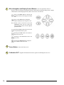
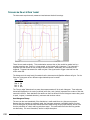
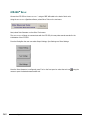
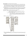
INITIAL DIALOG BAR
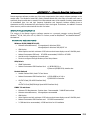
The initial Dialog Bar (see figure below) displays categories of tools (Clock, Data, Other Tools, etc.).
Each category contains one or more analysis tools to choose from. Once a tool is chosen, the Dialog Bar
will remain showing various pages of menus to control each tool. These configuration menus change to
reflect the selected tool window if more that one tool at a time is open.
Clicking on a button reveals the associated tool(s).
36
Section 4 - GigaView
©WAVECREST Corporation 2005
DIALOG BARS
Once a measurement tool has been chosen, the Dialog Bar displays general and tool-specific parameter
selections. Many of the tools have parameters common between them, such as Channel or Arming
Mode, while some of the GigaView tools have parameters unique to their function. For a detailed
explanation of a specific tool’s Dialog Bar parameters, see the Glossary section at the end of this manual
or use the context sensitive online Help system in GigaView.
The View menu lists data display
options and remains unchanged
throughout tool dialog pages.
Pop-up box for selecting channels.
User-selectable parameters
in active fields.
Scrolling menus list parameter and
function options.
©WAVECREST Corporation 2005
Section 4 - GigaView
37
This page intentionally left blank.
38
Section 4 - GigaView
©WAVECREST Corporation 2005
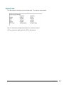
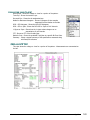
MEASUREMENT TOOLS
Oscilloscope - View the waveform
Clock - Single channel measurements
Clock Analysis - Combines different measurement tools.
Histogram - Statistical analysis of measurements such as period, pulse width, rise time, fall time.
Includes DJ and RJ separation using TailFit
High Frequency Modulation - View jitter accumulation or the spectral content of jitter.
Strip Chart - Plot histogram statistics at regular intervals defined by the user.
PLL Analysis - Extract information such as damping factor, natural frequency, input noise level, lock
range, lock-in time, pull-in time, pullout range and noise bandwidth.
Other Clock Tools
Statistics - Displays time measurements including frequency and duty cycle
Low Frequency Modulation - Power-up testing of PLL circuits; view low frequency jitter - below 20kHz.
Phase Noise - Create phase noise plots.
Locktime - Analyze PLL stabilization time.
Cycle-to-Cycle - Displays a histogram of the difference between two adjacent cycles of a clock.
DRCG - Characterize the effect of the second phase aligner stage of the DRCG on a cycle-by-cycle
basis as specified in the Rambus DRCG specification.
Spread Spectrum Clock - Automatically measures SSC effects on signals.
Channel-to-Channel
Propagation Delay and Skew - Histogram of measurement between 2 channels such as prop delay/skew.
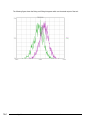
Data Bus - Characterize single-ended and differential clock and data signals.
Strip Chart - Plot histogram statistics at regular intervals defined by the user.
Data - Advanced clock-to-data analysis and extensive jitter analysis including DJ and RJ separation.
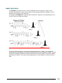
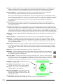
Known Pattern with Marker - Used to show jitter and its components on a data pattern relative to its ideal
bit position
Random Data with Bit Clock - Use bit clock as a trigger.
Random Data, no Marker - This tool analyzes a single data signal when there is no bit clock or marker.
Data Standards
PCI Express - Provides both timing and amplitude compliance measurements.
Fibre Channel - Automates measurements and provides pass/fail results.
Serial ATA - Automates jitter generation specification profile measurements and provides pass/fail results.
InfiniBand - Automates measurements and provides pass/fail results.
Other Tools - Utilize other
WAVECREST
products.
Jitter Generator (DTS-550) - Versatile clock generator.
Switch Matrix (DSM-16x) – Extends input capability of instrument.
Arm Generator (AG-100) - Produces a pattern marker from a repeating data pattern.
Optical to Electrical Converter (OE-2) - Converts optical communication signals into electrical signals
Pattern Marker (PM50) - On-board pattern marker; uses SIA-3000 channel card to produce pattern
marker from a repeating data pattern.
Pattern Tool - Identify, load or save repeating data pattern.
Folded Eye Diagram – Measure mask violations on repeating patterns.
Composite Plot - Overlay related plots. Accessed via the Toolbar (
©WAVECREST Corporation 2005
).
Section 4 - GigaView
39
This page intentionally left blank.
40
Section 4 - GigaView
©WAVECREST Corporation 2005
Oscilloscope Tool
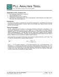
Applications
•
Display a waveform as voltage vs. time
•
Measure voltage parameters of signals
•
Measure Rise and Fall time
•
Eye mask measurements
Overview
The Oscilloscope Tool provides the user with a quick and easy graphical display of the signal to be
analyzed. The Oscilloscope has many different capabilities. It can display the waveform, measure
voltage parameters, and create eye masks.
Using the Oscilloscope Tool is similar to using any other oscilloscope. You can verify the signal using the
scope function before analyzing jitter. This eliminates the need to disconnect probes to use a separate
scope if the jitter results do not make sense.
©WAVECREST Corporation 2005
Section 4 - GigaView
41
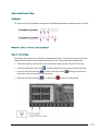
Oscilloscope Dialog Bars
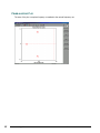
42
Section 4 - GigaView
(See the Glossary or Online Help for definitions of each field.)
©WAVECREST Corporation 2005
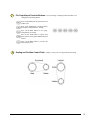
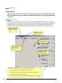
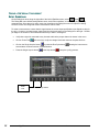
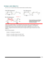
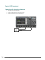
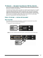
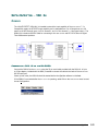
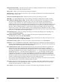
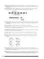
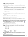
Making an Oscilloscope Measurement
Setup Directions
This tool requires a signal connected to any available measurement channel. A trigger signal can be
connected to any available channel, or the measurement can be triggered from the measurement channel.
•
Verify the proper input signal levels.
•
Connect the source to any IN channel.
•
Connect a trigger to any IN channel, add the channel and change the trigger/arm channel (see
instructions below). Or, you may select to trigger off of the signal on the measurement channel.
•
Press Pulsefind
•
Press Single Acquire
on the Tool Bar.
on the Tool Bar.
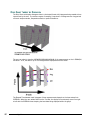
Device
Under
Test
Connect to IN of any channel.
Use trigger on any input.
Select measurement channel in dialog box.
Select arm channel in Trigger dialog box.
©WAVECREST Corporation 2005
Section 4 - GigaView
43
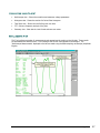
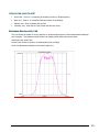
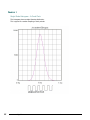
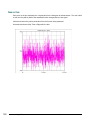
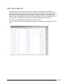
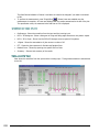
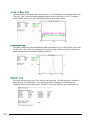
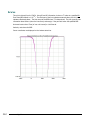
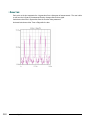
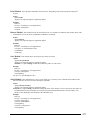
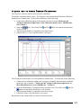
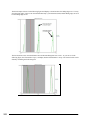
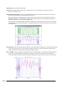
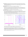
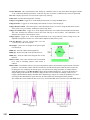
Interpreting Oscilloscope Views (plots)
•
Time - Time vs. Voltage including Eye Mask options.
•
Summary - Textual display of Oscilloscope measurements.
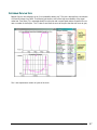
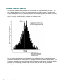
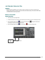
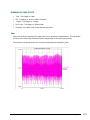
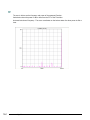
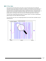
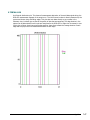
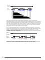
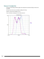
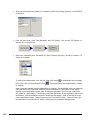
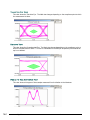
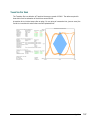
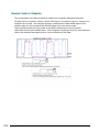
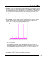
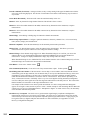
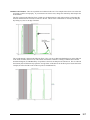
Time View with Eye Mask Enabled
To make an Eye Mask measurement, connect a data signal to one channel and a bit clock to another channel.
Set the trigger to be the channel with the bit-clock.
Press Signal Analysis, Eye Mask, then select ON in Enable Eye Mask.
Pressing Show Measures will display the number of samples on the display (Compares) and the number of
Violations of the mask regions. This is a toggle, and pressing it again will turn off those values.
Press Zoom to Eye to automatically place the mask in the display. To change the mask position or size, press
Mask Setup. This will allow you to configure the mask.
For other configuration and tool settings, refer to the context sensitive help. The help describes the use of
each setting.
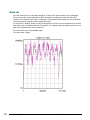
In Time View, resolution affects the time between measurements. Range affects the time over which
measurements are made.
44
Section 4 - GigaView
©WAVECREST Corporation 2005
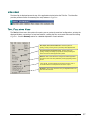
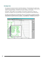
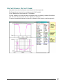
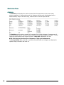
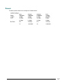
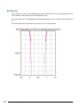
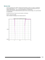
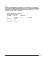
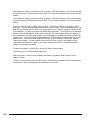
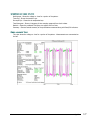
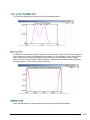
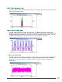
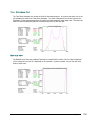
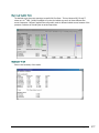
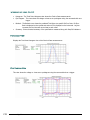
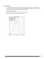
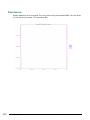
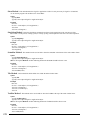
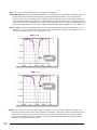
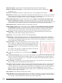
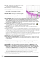
Summary View
The data represent information from the Oscilloscope. This page can be annotated.
Each row summarizes voltage measurements for a particular channel.
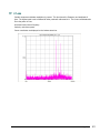
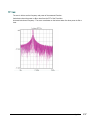
FFT-Fmax reports the tallest peak on the FFT for that channel.
©WAVECREST Corporation 2005
Section 4 - GigaView
45
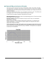
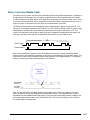
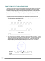
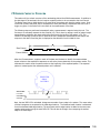
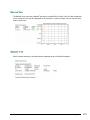
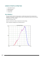
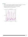
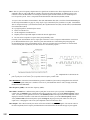
Oscilloscope Theory of Operation
There are two different measurement engines in the SIA-3000 that perform specific measurements using
the most appropriate hardware techniques. The Sampling Oscilloscope uses circuitry optimized for voltage
measurements (Amplitude Engine). Timing and Jitter measurements use different internal circuitry optimized
for time measurements (Timing Engine). For amplitude measurements and rise or fall time measurements
(which are amplitude dependent) the Oscilloscope uses a standard Repetitive Sampling methodology. This
allows eye-masks to be created. The time measurements made for the other tools, such as histogram, are
not derived from the measurements that this oscilloscope makes.
46
Section 4 - GigaView
©WAVECREST Corporation 2005
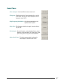
Clock Tools
Clock Analysis - Combines different measurement tools
Histogram - Statistical analysis of measurements such as period,
pulse width, rise time, fall time. Includes DJ and RJ
separation using TailFit.
High Frequency Modulation - View jitter accumulation or the
spectral content of jitter.
Strip Chart - Plot histogram statistics at regular intervals defined
by the user.
PLL Analysis - Extract information such as damping factor, natural
frequency, input noise level, lock range, lock-in time,
pull-in time, pull-out range and noise bandwidth.
Other Clock Tools - This button accesses other tools used for
clock analysis. See Other Clock Tools.
©WAVECREST Corporation 2005
Section 4 - GigaView
47
This page intentionally left blank.
48
Section 4 - GigaView
©WAVECREST Corporation 2005
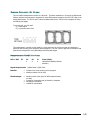
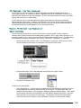
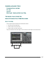
Clock Analysis Tool
This tool combines a few different measurement tools in the SIA-3000. By doing this, a large number of
useful results can be displayed quickly. The Measure Option button allows you to toggle on or off certain
measurements. The measurement settings provide the best configuration to a variety of users. This ease
of use means that there is less control over individual settings. There may be instances where there is
the need to have more control over a specific measurement. An example would be changing the trigger
delay on the oscilloscope, or measuring a histogram over two periods rather than single period jitter.
Another example would be to find very low frequency jitter below the (clock/1667) low cutoff frequency
of this tool.
In any of these cases, you can press Current View Diagnostic Tool from the view you are in to open that
specific tool, make the measurement and have control over a larger number of settings. If viewing the
Oscilloscope view, Pressing "Current View Diagnostic Tool" will open the Oscilloscope tool. You now have
access to many more configuration settings. If viewing the Histogram view, Pressing "Current View
Diagnostic Tool" will open the Histogram tool and allow different settings.
This tool has a variety of views. The displayed results are determined by the selections in the Measure
Options menu. The default is to perform all measurements.
©WAVECREST Corporation 2005
Section 4 - GigaView
49
Making a Clock Analysis Measurement
Setup Directions
•
Connect signal to Channel 1.
Most Tools default to Channel 1, however, the input channel can be changed. For single-ended
measurements, use just the top input SMA leaving the bottom unconnected. For differential
measurements, connect to Input and Input-.
•
Open the Clock Analysis tool by selecting the Clock and Clock Analysis buttons.
•
Press Single/Acquire
on the toolbar or the Single/Acquire button on the front panel. Some results
require repeated runs to acquire; you can press Run
to get those values.
See Interpreting Clock Analysis Views for descriptions of the different ways of displaying the measurements
made by the Clock Analysis Tool.
50
Section 4 - GigaView
©WAVECREST Corporation 2005
Interpreting views (plots)
•
Oscilloscope view – Shows the waveform and measures voltage parameters.
•
Histogram view - Shows the results of a Period Jitter histogram.
•
Total Jitter view - Shows how the Pk-Pk grows over time.
•
FFT – Shows a frequency analysis of the jitter.
•
Summary view - View data in a text format and save user notes.
Oscilloscope View
This Tool performs a number of measurements and summarizes the results on the left side. These results
are associated with different Views. In this example the Current View selected is Oscilloscope. The
"Oscilloscope Measurements" displayed to the left are made using the 6GHz sampling oscilloscope (Amplitude
Engine).
©WAVECREST Corporation 2005
Section 4 - GigaView
51
Histogram View
The Histogram View shows the results of a Period Jitter histogram. The Period samples are made from the
rising edge to the rising edge of a single period (using Timing Engine). The Period Mean, 1-Sigma and Pk-Pk
relate to the displayed histogram. Period Hits is the number of samples in the histogram.
Pulse Width+ and Pulse Width- are also calculated from a histogram of measurements—though, this
histogram is not displayed. Duty cycle and Frequency can then be calculated from these measurements.
The values for RJ (Random Jitter), DJ (Deterministic Jitter) and TJ (Total Jitter) are calculated using TailFit.
TailFit determines an accurate RJ when DJ is present. TJ is a predicted Pk-Pk value based on the RJ and DJ
measured and is bounded at some level of probability or some elapsed time. The default for this is 1e-12.
52
Section 4 - GigaView
©WAVECREST Corporation 2005
Total Jitter View
The Total Jitter View shows how the Pk-Pk grows over time. Pk-Pk of a histogram is not a meaningful metric
if not bounded in some way. There are various bounds that can be used, such as sample size or acquisition
time. The SIA-3000 defaults to a bound of 1e-12 level of probability. This means that TJ is the predicted PkPk of a histogram at some point in time. The point where the color changes to gray is the bound for the TJ
(this can be changed).
The Total Jitter View shows three lines. The vertical axis is the Total Jitter. The horizontal axis is elapsed
time. The highest line is the Total Jitter predicted from TailFit (See TailFit Theory, Appendix B). The other
two lines show the jitter for Short periods and Long periods.
For a detailed description of the Histogram Measurement Theory, refer to the Histogram Getting Started
Guide.
©WAVECREST Corporation 2005
Section 4 - GigaView
53
FFT View
The FFT view shows a frequency analysis of the jitter. When Deterministic Jitter is present, it is often
periodic and can be identified in this jitter spectrum view. The summary on the left shows the amplitude of
the largest Periodic Jitter (PJ pk-pk) spike. The frequency of the spike is labeled 'Pjfreq'. By identifying and
trying to remove the cause of the largest spikes will reduce overall Deterministic Jitter.
This measurement has a fixed –3dB Corner Frequency High Pass Filter that is Fcarrier/1667. Frequencies below
this will be significantly attenuated.
For a detailed description of the underlying theory of this measurement, refer to the "High Frequency
Modulation Getting Started Guide".
54
Section 4 - GigaView
©WAVECREST Corporation 2005
Clock Analysis Theory
The SIA-3000 is a hybrid instrument that combines the measurement capabilities of a sampling
oscilloscope with time measurement circuitry: Rise/Fall times, Voltage amplitude and Eye Masks from the
Oscilloscope; timing parameters, i.e., Period, Pulse widths, Skews and components of Jitter from the time
measurement circuitry. This tool combines a few different measurement tools in the SIA-3000. By doing
this, a large number of useful results can be displayed quickly. The "Measure Options" button allows you to
toggle on or off certain measurements. The measurement settings provide the best configuration to a variety
of users. This ease of use means that there is less control over individual settings. But, there may be
instances where there is the need to have more control over a specific measurement. Some examples would
be changing the trigger delay on the oscilloscope, or measuring a histogram over two periods rather than
single period jitter. Another example would be to find very low frequency jitter below the (clock/1667) low
cutoff frequency of this tool.
In any of these cases, you can press "Current View Diagnostic Tool" from the view you are in to open that
specific tool, make the measurement and have control over a larger number of settings. If viewing the
Oscilloscope view, Pressing "Current View Diagnostic Tool" will open the Oscilloscope tool. You now have
access to many more configuration settings. If viewing the Histogram view, Pressing "Current View
Diagnostic Tool" will open the Histogram tool and allow different settings.
©WAVECREST Corporation 2005
Section 4 - GigaView
55
This page intentionally left blank.
56
Section 4 - GigaView
©WAVECREST Corporation 2005
Histogram Tool
Applications of Histogram Tool
•
Displays information about the distribution of the measured events such as period, Rise time, Fall
time, Positive pulse width, and Negative pulse width.
•
Displays a histogram of the samples taken during a single burst of measurements.
•
Analysis of long-term signal integrity in a short test time. TailFit option separates the Gaussian and
deterministic components from the measured distribution. For a multi-modal distribution, Tailfit gives
accurate information about the effects of jitter on long term and short term signal integrity.
The Histogram tool provides the user with statistical analysis of time measurements of different clock
features such as Period, Rise time, Fall time, Positive Pulse Width, Negative Pulse Width. The time
measurements are asynchronously sampled at random intervals to give a solid, statistical set displayed
as an Histogram. The values of Mean, Maximum, Minimum, Peak-to-peak and 1-sigma are reported.
Proprietary software algorithms separate deterministic and random jitter components allowing the
calculation of total jitter. These values are used to create a Bathtub Curve to predict long-term reliability.
See also TailFit theory, Appendix B.
©WAVECREST Corporation 2005
Section 4 - GigaView
57
Making a Histogram Measurement
Setup Directions
On the Dialog bar menu along the right side of the initial GigaView screen, select
, then
.
The Dialog Bar menu default settings allows users, under most conditions, to immediately begin making
measurements. Once the tool is open, users may reconfigure the Dialog bar menus for optimum viewing.
Once the menus are configured a basic measurement can be made.
To make a measurement, ensure that the signal meets the current input specifications (see Signal Levels) for
the unit. Connect to a measurement channel and choose that channel on the Dialog bar to the right. Set Hits
per Edge to the number of time measurements that you want in a histogram.
•
Verify that a signal is connected to any channel and that the proper channel is chosen in the menu.
•
Click on Pulse Find
•
Click on the Single Acquire button
or press the Run/Cycle button
accumulate a continuous series of measurements.
•
Press the Single Acquire button
Device
Under
Test
58
Section 4 - GigaView
on the tool bar. Verify the voltage levels and close out the pulse find box.
or the Stop button
allowing the instrument to
to stop the cycling process.
Connect to IN of any channel.
©WAVECREST Corporation 2005
Interpreting views (plots)
•
Acum view - Time vs. # of samples (all samples from Run or Single acquires)
•
Maxi view - Time vs. # of samples (Maximum extent of all samples)
•
Bathtub view - Error Probability Density Plot
•
Summary view - View data in a text format and save user notes
Histogram Accumulated View
This view shows the results of running acquires or multiple single acquires of time measurements displayed
as a histogram. The statistics and plot relate to all measurements taken since the last clear.
Horizontal x-axis shows Time.
Vertical y-axis shows the number of measurements (Hits per Edge).
Cursor coordinates are displayed on the bottom status line.
©WAVECREST Corporation 2005
Section 4 - GigaView
59
Histogram Maxi View
This view shows the Maximum number of hits per edge displayed as a histogram. Multiple acquires will only
change the plot if the hits per edge for a given time exceeded the values from a previous acquire. It can be
thought of as a maximum envelope of time measurements.
Horizontal x-axis shows Time.
Vertical y-axis shows the number of measurements (Hits per Edge).
Cursor coordinates are displayed on the bottom status line.
60
Section 4 - GigaView
©WAVECREST Corporation 2005
Histogram Bathtub View
Bathtub Curve is also referred to as an "error probability density plot." This plot is derived from a convolution
of DJ and RJ values from TailFit. The following plot shows a view of the long-term reliability of the signal
under test. Total Jitter (TJ) is extracted directly from this plot and is a peak-peak value at a specific bit error
rate or number of clock cycles. The TJ value is read from the curve at the point that the color turns to gray.
The Y-axis represents a number of cycles of the clock.
©WAVECREST Corporation 2005
Section 4 - GigaView
61
Histogram Summary View
The data represent values from histograms of measurements. Normal Histogram shows statistics from a
single histogram. Accumulated Histogram shows statistics from all histograms since a clear. The user is able
to annotate this page.
If TailFit is enabled, additional values are shown:
- LRMS, RRMS, AvgRMS, DJ, TJ and Goodness of Fits
- LRMS is the RMS value from the Gaussian fitted to the left tail.
- RRMS is the RMS value from the Gaussian fitted to the right tail.
- AvgRMS is the average of the LRMS and RRMS values.
- DJ is calculated between the means of the fitted Gaussians on the histogram.
- TJ is calculated from the RJ and DJ components at a specific BER.
- Goodness of Fits is CHI Square value. Lower numbers indicate better confidence in RJ values.
See TailFit Theory, Appendix B.
62
Section 4 - GigaView
©WAVECREST Corporation 2005
With TailFit Enabled - See TailFit Theory
Accumulated view shows the Gaussian curves fitted to the left and right tails.
This Example shows three views from a histogram with TailFit enabled:
The top, Bathtub curve shows where the TJ is calculated.
The right, Summary view shows the values for goodness-of-fits (Chi-Squared), extracted DJ and fitted
rmsJ. The rmsJ values are smaller than the 1-sigma for the histogram.
The bottom, Accumulated Histogram View shows the Gaussian curves fitted to the left and right tails.
©WAVECREST Corporation 2005
Section 4 - GigaView
63
Histogram Theory of Operation
The Histogram is the most basic information that the instrument and GigaView software will provide. The
Hits per Measure determines how many time measurements will be in each histogram. Time values are
binned and displayed on the x-axis (horizontal) while the y-axis (vertical) represents the number of hits that
occurred in that bin. Basic statistical information can then be derived from the histogram: mean value, peakto-peak, 1-sigma (1 standard deviation), maximum and minimum values.
The user can also see immediately if the distribution is multi-modal and if there is a jitter source present.
Because the time samples are randomly made, the histogram represents a probability density function. So if
the histogram of periods were bimodal with each mode having roughly equal samples, we can infer that the
probability of a short and long period are equal. This would mean that short and long periods are
alternating. For more information, see the in-depth description.
64
Section 4 - GigaView
©WAVECREST Corporation 2005
Histogram In-depth Description
The SIA-3000™ asynchronously measures times between threshold crossings.
fall time = t2
These "hits" are made randomly. This randomization ensures that no jitter would be masked out by a
constant sampling rate. Each hit, or time sample, is then binned into a histogram. The histogram is
complete once the number of Hits per Measure has been reached. Additionally, the SIA-3000™ is not
triggered. Triggered instruments can mask out jitter if the signal used to trigger is derived from the circuit
under test.
See the following examples:
Example 1 is a histogram of a good clock.
Example 2 is a bimodal histogram with equal heights.
Example 3 is a bimodal histogram with unequal heights.
©WAVECREST Corporation 2005
Section 4 - GigaView
65
Example 1
Single Mode Histogram - A Good Clock
This histogram shows a single Gaussian distribution.
This is typical of a random sampling of clock periods.
66
Section 4 - GigaView
©WAVECREST Corporation 2005
Example 2
Bimodal Histogram-Equal Heights
This histogram shows two distributions (modes) that have roughly equal amounts of hits. The histogram
relates to the probability of times being measured. Equal numbers of hits means that there is a equal
probability (50%-50%) of measuring either short or long times (periods in this example). So in reality the
clock would be alternating short, long, short, long, etc.
©WAVECREST Corporation 2005
Section 4 - GigaView
67
Example 3
Bimodal Histogram - Unequal Heights
This histogram shows two distributions (modes) that have unequal amounts of hits. The histogram relates to
the probability of times being measured. Unequal numbers of hits means that there is an unequal probability
of measuring short or long times (periods in this example). Here, the left mode has four times as many
samples as the right mode. The associated probabilities are 75% and 25% respectively. So in reality the
clock would have three short periods and one long.
68
Section 4 - GigaView
©WAVECREST Corporation 2005
High Frequency Modulation Tool
Applications
•
•
•
•
View accumulated jitter in the modulation domain
Look at the frequency components of jitter using an FFT
Determine the amplitude, power or relative contribution to total jitter of each spectral component
View how the jitter changes over time or output cycles.
Overview
High Frequency Modulation Analysis allows the user to see jitter accumulation or spectral content of the jitter.
HF Modulation Analysis compiles histograms of incrementally increasing consecutive period measurements.
These measurements can be between rising or falling edges. The High Frequency modulation tool plots a
peak-peak value for an edge versus time. See High Frequency Modulation Theory.
High Frequency Modulation Dialog Bar
©WAVECREST Corporation 2005
Section 4 - GigaView
69
Making a Measurement
Setup Directions
On the Dialog bar menu along the right side of the initial GigaView screen, select
then
.
The Dialog Bar menu default settings permits users, under most conditions, to immediately begin making
measurements. Once the tool is open, users may reconfigure the Dialog bar menus for optimum viewing.
Once the menus are configured a basic measurement can be made.
To make a measurement, ensure that the signal meets the current input specifications (see Signal Levels) for
the unit.
•
Verify that a signal is connected to an input channel and that the proper channel is chosen in the Dialog
bar menu to the right.
•
On the top toolbar press Pulse Find
•
or press the Run/Cycle button
Press the Single Acquire button
accumulate a continuous series of measurements.
•
Press the Single Acquire button
Device
Under
Test
. Verify the voltage levels and close out the pulse find box.
or the Stop button
allowing the instrument to
to stop the cycling process.
PLL, Clock or Oscillator Output.
Connect to IN of any channel.
All of the measurements and data required to calculate and display the different views or plots available in
the High Frequency Modulation tool are gathered simultaneously on one pass or acquisition.
70
Section 4 - GigaView
©WAVECREST Corporation 2005
Interpreting views (plots)
•
1-Sigma view - Edges (or time) vs. 1-sigma
•
Pk-Pk view - Edges (or time) vs. 1-sigma
•
FFT N-clock view - Frequency vs. power
•
FFT 1-clock view - Frequency vs. power (N-clock FFT with 20dB/decade Low Frequency roll-off)
•
Summary view - View data in a text format and save user notes
1-Sigma View
Each point on the plot represents the 1-sigma value from a histogram of measurements. The user is able
to see how the 1-sigma value changes relative to accumulating clock periods. This provides information
about jitter accumulation.
Horizontal x-axis shows either Time or number of Edges over which a histogram is made.
Vertical y-axis shows the 1-sigma value.
Cursor coordinates are displayed on the bottom status line
This plot shows the accumulation of jitter. Periodic components indicate modulation is present.
The frequency and power of this jitter can then be seen in the FFT View.
©WAVECREST Corporation 2005
Section 4 - GigaView
71
Peak-to-Peak View
Each point on the plot represents the peak-to-peak value from a histogram of measurements. The user
is able to see how the peak-to-peak value changes relative to accumulating clock periods.
Horizontal x-axis shows either Time or number of Edges over which a histogram is made.
Vertical y-axis shows the peak-to-peak value.
Cursor coordinates are displayed on the bottom status line.
72
Section 4 - GigaView
©WAVECREST Corporation 2005
FFT N-clock view
The user is able to see the frequency components and amplitude of the jitter.
Horizontal x-axis shows Frequency.
Vertical y-axis shows the power in dBs or time.
Cursor coordinates are displayed on the bottom status line.
©WAVECREST Corporation 2005
Section 4 - GigaView
73
FFT 1-clock view
The user is able to see the frequency components and amplitude of the jitter affecting a single clock
period. Compared to the N-clock view, the 1-clock view has a 20dB/decade roll-off for low frequencies.
The purpose of this is to show the effect of jitter on a single clock period. Low frequency jitter
components will affect single cycles of a clock much less than higher frequency jitter components.
Horizontal x-axis shows Frequency.
Vertical y-axis shows the power in dBs or time.
Cursor coordinates are displayed on the bottom status line.
74
Section 4 - GigaView
©WAVECREST Corporation 2005
Summary View
The data represents values from histograms of measurements.
-The values in the 1-sigma row show the mean/min/max and pk-pk 1-sigma values from the 1-sigma plot.
-The values in the pk-pk row come from the pk-pk plot and show the mean, max and pk-pk of the pk-pk values.
-1-clock PJ and Freq show only the highest peak from the FFT (1-clock) view.
-N-clock PJ and Freq show only the highest peak from the FFT (n-clock) view.
-RJ is RMS jitter between -3dB Freq and Fmax
©WAVECREST Corporation 2005
Section 4 - GigaView
75
High Frequency Modulation Theory
The High Frequency Modulation Analysis tool enables the user to see jitter accumulation and frequency
components of the jitter. This tool acquires data by creating many histograms of measurements. Each
histogram contains successively increasing numbers of periods. For example, a histogram of single
periods is made, then a histogram of two periods, then three and so forth. By plotting the 1-sigma
values relative to the number of periods, a comparison is made between histograms. When jitter is
present, the 1-sigma values will change periodically. Frequency information can be derived from the
changing 1-sigma values by using a windowed FFT.
Setting the -3dB Lower Rolloff Frequency to the lowest jitter frequency that you are concerned with will
determine the number of histograms that must be made. The Fmax divider allows you to scale the FFT
accordingly.
76
Section 4 - GigaView
©WAVECREST Corporation 2005
Strip Chart Tool
Overview
The Strip Chart tool plots histogram statistics at regular intervals defined by the user. The user can select
to view the AVERAGE of the measurements and/or the AVERAGE, plus the RMS Jitter or the ± peak jitter.
This is selected in the View pull-down menu. The most vertical data represents the highest one-shot
measurement of jitter and the lowest line being the most negative one-shot measurement of jitter. The
line in the middle is the measurement AVERAGE of all the data taken by the instrument.
The "Elapsed Seconds" displayed on the horizontal scale indicates the time over which the burst results
are graphically being displayed. In all, the data for up to 500 bursts are displayed across the screen.
The Elapsed Time for those 500 bursts depends on the time entered into "Interval(s)", which is on the
Dialog Bar. When the user selects "Cycle" from the Tool Bar, the display will continuously move from
right to left with the "Elapsed Seconds" time stamping the burst data being displayed within the graph.
This allows long-term effects, such as environmental effects of long-term drift, to be measured. For
example, histograms of period measurements could be made at every interval, i.e. 10 minutes, and the
mean, 1-sigma, pk-pk, and max/min values plotted over a long time, i.e. overnight.
Making a Measurement
Setup Directions
•
Verify the proper input signal levels.
•
Connect the source to any channel IN
•
If using External Arm Mode, connect an Arm signal to an input channel and select the appropriate
channel in the Arming dialog bar
Device
Under
Test
Connect to IN of any channel.
©WAVECREST Corporation 2005
Section 4 - GigaView
77
Interpreting Strip Chart Views (plots)
•
Ave/Max/Min
•
Pk-Pk/1-Sigma
•
Summary
Ave/Max/Min
See long term changes in the Average, Maximum and Minimum measured values.
Horizontal x-axis shows time. The time Increment between points is set by the user.
Vertical y-axis shows the measured time.
The top line represents the Maximum; middle line, the Average; and bottom line, the Minimum values
from histograms.
Cursor coordinates are displayed on the bottom status line.
78
Section 4 - GigaView
©WAVECREST Corporation 2005
1-Sigma View/Pk-Pk
See long-term changes in the Peak-to-Peak and 1-sigma measured values.
Horizontal x-axis shows time. The user sets the increment between points.
Vertical y-axis shows the measured time.
The top line represents the Peak-to-Peak values and the bottom line shows the 1-sigma values from
histograms.
Cursor coordinates are displayed on the bottom status line.
Summary View
Shows the statistics from the most recent histogram.
©WAVECREST Corporation 2005
Section 4 - GigaView
79
Strip Chart Theory of Operation
The Strip Chart tool displays histogram data in a horizontal format with histograms being created at time
intervals set by the user. It provides a means of compiling "snap-shots" of histograms over long periods
of time to analyze wander, temperature effects or power fluctuations.
The user can select to view the AVERAGE/MINIMUM/MAXIMUM of the measurements or the 1-SIGMA/PKPK values. In all, the data for up to 500 histograms are displayed across the screen.
The Elapsed Time between each histogram of time measurements depends on the time entered into
INTERVAL. When the user selects RUN from the Tool Bar, the display will continuously move from right
to left with the INTERVAL time stamping the burst data being displayed within the graph.
80
Section 4 - GigaView
©WAVECREST Corporation 2005
PLL Analysis Tool
Applications of the PLL Analysis Tool
•
Find the transfer function of a 2nd-order PLL
•
View the Bode plot of a PLL.
•
Identify poles and zero of a 2nd-order PLL.
•
Determine PLL characteristics such as lock in damping factor, natural frequency, lock range, lock-in time,
pull-in time, pull-out range, etc.
Overview
The PLL Analysis tool permits users to study characteristics and parameters of a 2nd-order PLL. With a
simple set of variance measurements, the tool can extract information such as damping factor, natural
frequency, input noise level, lock range, lock-in time, pull-in time, pull-out range and noise bandwidth.
The tool also presents a transfer function and Bode plots up to the natural frequency, as well as a plot of
the poles and zero for a 2nd-order PLL.
©WAVECREST Corporation 2005
Section 4 - GigaView
81
Making A PLL Analysis Measurement
Setup Directions
•
Open the Advanced PLL tool.
•
Connect the signal to a measurement channel (see below). Set the measurement channel in
GigaView by going to the Acquire Option menu and choosing Channel.
•
Confirm that a valid signal exists at the measurement channel by using Pulsefind
•
Set the Rec Length (µs) and the Meas Incr (Periods). All other parameters are left as default.
•
Begin acquisition by pressing Single/Stop button on the front panel
.
.
When acquisition is complete, the Single/Stop button will cease to illuminate.
82
Section 4 - GigaView
©WAVECREST Corporation 2005
Interpreting PLL Analysis views (plots)
•
1-Sigma
•
PLL Transfer
•
Bode Plot
•
Poles & Zero
•
Summary
1-Sigma Plot
The time domain data can be viewed by selecting 1-Sigma under the View menu.
The x-axis shows the span of the jitter accumulation. The y-axis shows the rms standard deviation of the
accumulated jitter at a certain span.
©WAVECREST Corporation 2005
Section 4 - GigaView
83
PLL Transfer Plot
The domain of the transfer function is frequency normalized to the natural frequency
magnitude in dB.
84
Section 4 - GigaView
ωn .
The y-axis is
©WAVECREST Corporation 2005
Bode Plot
The domain of the Bode Plot is frequency normalized to the natural frequency
amplitude in dB and the lower plot is phase in degrees.
©WAVECREST Corporation 2005
ωn .
The upper plot is
Section 4 - GigaView
85
Poles and Zero Plot
The axes of the plot is complex frequency normalized to the natural frequency
86
Section 4 - GigaView
ωn .
©WAVECREST Corporation 2005
Summary Plot
This view contains many calculated PLL characteristics such as damping factor, natural frequency, input
noise level, lock range, lock-in time, pull-in time, pull-out range, and noise bandwidth.
Data summary and PLL characteristics
The PLL characteristics provided in the summary window are the following:
• Damping factor – ζ as defined in Eq. 1 (see PLL Analysis Theory).
• Natural frequency – ωn as defined in Eq. 1.
• PSD of noise – level of white input noise.
• Lock range – frequency range within which a PLL can lock within one beat note between the ωRef and ωOut.
• Lock-in time – time scale for PLL to lock into from the lock range.
• Pull-in time – time scale for the PLL to lock from the pull-in range, which is the range within which the
PLL will always lock.
• Pull-out range – the dynamic limit for stable operation of a PLL.
• Noise bandwidth – PLL output phase noise integrated over the bandwidth of the PLL
©WAVECREST Corporation 2005
Section 4 - GigaView
87
PLL Analysis Theory of Operation
The PLL Analysis measurement tool is based on a white paper authored by WAVECREST Corporation [1].
The fundamental measurement of this tool is the 1-sigma (σ ) vs. UI plot similar to the High Frequency
Modulation tool [2]. The relationship between the jitter variance (σ2) and the jitter power spectral
density (PSD) is well established [3]. The jitter PSD of the PLL output clock is related to the PLL
reference clock noise via the transfer function. Therefore, with reasonable assumptions about the input
noise of the PLL reference clock, we can infer the transfer function of the PLL.
At the current time, we assume that the input noise spectrum is white and the PLL is of 2nd-order. The
2nd-order PLL transfer function in Laplace space is given by
H (s) =
2ζωn s + ωn2
s 2 + 2ζωn s + ωn2
s = iω is the complex frequency, ωn is the natural frequency, and ζ is the damping factor. The
parameters ωn, ζ, and the input noise level are found from a least-squares fit of the variance. Once
H(s) is determined, PLL characteristics such as natural frequency, damping factor, damping frequency,
where
pull-in range, pull-in time, pull-out range, pull-out time, lock range, lock time, lock frequency, Bode plots,
root locus, poles, zeros, and stability are readily obtained.
[1] Li, M., A New Method for Simultaneously Measuring and Analyzing PLL Transfer Function and Noise
Processes, DesignCon Proceedings, 2002.
[2] For more information, refer to "High Frequency Modulation", GigaView Quick Reference Guide,
Wavecrest Corporation
[3] Wilstrup, J., A Method of Serial Data Jitter Analysis Using One-shot Time Interval Measurements, ITC
Proceedings, p.819, 1998.
88
Section 4 - GigaView
©WAVECREST Corporation 2005
OTHER CLOCK TOOLS
Statistics - Displays time measurements including frequency and duty cycle.
Low Frequency Modulation - Power-up testing of PLL circuits; view low
frequency jitter - below 20kHz.
Phase Noise - Show the amplitude and frequency of phase noise relative
to the carrier signal frequency.
Locktime - Analyze PLL stabilization time.
Cycle-to-Cycle - Displays a histogram of the difference between two adjacent
cycles of a clock.
DRCG - Analyze, debug and characterization of clock signals using Adjacent Cycle
Jitter Statistics as required for Rambus DRCG devices.
Spread Spectrum - Automatically measures SSC effects on signals. The tool
will measure the frequency of the SSC as well as its plus
and minus parts per million (ppm) delta from a nominal
frequency.
©WAVECREST Corporation 2005
Section 4 - GigaView
89
Statistics Tool
Overview
The Statistics panel displays the results of several basic clock parameters in text format: mean,
minimum, maximum, 1-sigma, peak-to-peak, hits, frequency and duty cycle. Also displayed are the
measured Vstart, Vstop as well as the Vp-p, Vmax and Vmin of the two input channels.
The Statistics panel provides a summary of the statistics from a single histogram of measurements of
the chosen function (period, rise-time, fall-time, positive pulse width and negative pulse width). The tool
reports the clock frequency with 9 digits of precision. Duty cycle is displayed in this tool.
NOTE: This is the only tool that gives a frequency or duty cycle measurement.
The force pulsefind option, when set on, performs a pulsefind after each histogram and displays the
updated voltage information with each run.
90
Section 4 - GigaView
©WAVECREST Corporation 2005
Low Frequency Modulation Tool
Overview
The Low Frequency Modulation Tool is useful for power-up testing of PLL circuits or measuring low
frequency jitter problems (<20kHz), both synchronously and asynchronously, with either the AUTO ARM
or EXTERNAL ARM modes being enabled.
Making a Measurement
Setup Directions
•
Verify the proper input signal levels
•
Connect the source to any input and verify that the proper channel is chosen in the dialog bar menu.
•
or press the Run/Cycle button
Press the Single Acquire button
accumulate a continuous series of measurements.
•
Press the Single Acquire button
Device
Under
Test
or the Stop button
allowing the instrument to
to stop the cycling process.
Connect to IN of any channel.
©WAVECREST Corporation 2005
Section 4 - GigaView
91
Interpreting views (plots)
•
Time – Edges (or time) vs. time
•
FFT 1-clock - Frequency vs. power (N-clock FFT with 20dB/decade Low Frequency roll-off)
•
FFT N-clock – Frequency vs. power
•
Summary - View data in a text format and save user notes
Time
This view shows the modulation waveform.
The X-axis shows a timestamp value.
The y-axis shows the measured period value.
Cursor coordinates are displayed on the bottom status line
92
Section 4 - GigaView
©WAVECREST Corporation 2005
FFT 1-Clock
Periodic components indicate modulation is present. This plot shows the Frequency and amplitude of
jitter. The highest peak is set to 0dB and all other peaks are referenced to it. The cursor coordinates also
show the power in time.
Horizontal x-axis shows frequency.
Vertical y-axis shows power.
Cursor coordinates are displayed on the bottom status line.
©WAVECREST Corporation 2005
Section 4 - GigaView
93
Summary
This view shows a summary of the most recent time measurements and the frequency information from
the largest peak on the FFT
94
Section 4 - GigaView
©WAVECREST Corporation 2005
Low Frequency Modulation Theory of Operation
This circuitry is used to record the time at which a measurement is made, in other words, each single
time measurement in a histogram is time stamped. A single histogram of a number of hits is gathered.
The statistical values from this histogram are recorded in the Summary view. The data in this tool is not
plotted as a histogram.
In Time View, the single measurements, or hits, are plotted in the order they occur. The software plots
the timestamp value on the x-axis and the measured period value on the y-axis.
In the FFT View, the frequency information is derived from the Time View.
Minimum Data Points determines the number of time measurements shown on Time View and refers
to the number of hits in the histogram.
Maximum Frequency determines the resolution of the plot in the FFT view or the time between
measurements in Time View.
Basically, changing the Maximum Frequency slows down the sampling rate—or increases the time
between measurements. The instrument then captures samples over a longer time and is able to
measure lower frequency information.
The first example shows 10 measurements spaced in time. This represents a single histogram of 10 hits
with the hits plotted on the x-axis in the order they were acquired starting from the left. It is apparent
that the period of the clock being measured is varying or modulated. This acquisition has not captured
an entire cycle of the modulation.
©WAVECREST Corporation 2005
Section 4 - GigaView
95
By decreasing the Maximum Frequency, the time between measurements is increased and lower jitter
frequencies can be captured. The following figure shows the Maximum Frequency divided by two with
the same number of Minimum Data Points, 10, as in the previous figure.
Figure 2
96
Section 4 - GigaView
©WAVECREST Corporation 2005
Phase Noise Tool
Overview
The Phase Noise tool allows users to measure phase noise in clock/oscillator sources. By simply choosing
the highest frequency to be displayed and the frequency resolution, the tool will measure and display the
phase noise spectrum. A summary view reports the phase noise values at common offset frequencies.
The Phase Noise tool is used to show the amplitude and frequency of phase noise relative to the carrier
signal frequency. This tool measures the fluctuations in the phase of a signal caused by time domain
instabilities. Fast and easy phase noise measurements of oscillators and PLL devices can be easily
correlated to other noise effects on the signal.
Making a Measurement
Setup Directions
The signal that is being analyzed can be connected to any input channel.
•
Verify the proper input signal levels
•
Connect the source to IN of any channel
Device
Under
Test
Connect to IN of any channel.
©WAVECREST Corporation 2005
Section 4 - GigaView
97
Interpreting views (plots)
•
FFT - Time amplitude vs. frequency content of jitter
•
Summary - View data in a text format and save user notes
FFT View
This is the FFT of the acquired data. This plot shows the spectral power density of the jitter component
frequencies from the carrier frequency to the Maximum Frequency entered in the options.
In the following plot example, a phase noise measurement is made on a clock signal with injected phase
noise.
The signal source is a Marconi 2041 low noise signal generator. The signal has a carrier frequency of f0
= 1 GHz. The carrier is frequency modulated with white noise and deviation of ∆f = 50 kHz.
The bright magenta line is the phase noise measurement of the carrier with noise added. The dim
magenta line is the same measurement without noise and corresponds to the ~1/f noise floor of the
instrument.
The x-axis shows the frequency offset from the carrier.
The y-axis shows the measured phase noise.
98
Section 4 - GigaView
©WAVECREST Corporation 2005
Summary View
The Phase Noise Summary view reports values from acquired measurements.
Mean is the measured period time; note that if the Maximum Frequency setting is changed, this will
effectively skip edges and measure over many periods.
Min, Max, Pk-Pk, and 1-sigma are values from the histogram of measurements that the mean came from.
dBc/Hz is the reported value from the chosen offset frequency and offset width.
©WAVECREST Corporation 2005
Section 4 - GigaView
99
Phase Noise Theory
a)
b)
Power
Carrier
Phase Noise
f0
Phase Noise (dBc/Hz)
Phase noise is the random fluctuation of phase in a clock signal and is typically used to specify the quality
of a PLL circuit. In the frequency domain, phase noise appears as sidebands of the carrier frequency
(Figure a). Phase noise is commonly shown as a single side band at frequencies offset from the carrier
(Figure b). Typical domain of interest is frequencies within a few kilohertz of the carrier.
Frequency
Offset Frequency (Hz)
Figures a and b. Phase noise in frequency domain.
Phase noise is expressed as the normalized power spectral density (PSD) on a decibel scale. It is defined by
Eq. 1
 P( f ) 
 ,
L( f ) = 10 log10 
 P0 ∆f 
where f is frequency offset from the carrier, P0 is the power of the carrier, P(f) is the noise power
spectrum, and ∆f is the resolution bandwidth of the noise power spectrum. The units of phase noise are
dBc/Hz. Typical regions of interest are frequencies within a few kilohertz offset from the carrier. For the
time interval measurement systems, the phase noise power is given by
Eq. 2
1
2
P( f ) = V02 (2πf 0 ∆t ( f )) ,
2
where, f0 and V0 are the carrier frequency and peak voltage, respectively, and ∆t(f) is the FFT N-clock
jitter spectrum acquired from the Low Frequency Modulation tool. The power of the carrier is P0 = V02/2.
The corresponding phase noise is
Eq. 3
 f 2 ∆t ( f )2 
,
L( f ) = 10 log10  c

∆f


where ∆f is the resolution bandwidth of the jitter spectrum.
100
Section 4 - GigaView
©WAVECREST Corporation 2005
Locktime Tool
Applications
•
Measure Locktime or PLL settling time.
•
View the synchronous jitter.
•
Locktime Tool enables the user to view information about the measured function of the signal on the
measurement channel with respect to some arming point. The user can view any synchronous jitter
pattern that may exist. View the frequency or period settling time of a PLL after a change, such as a
lock signal or input frequency change.
Overview
The Locktime tool is actually an automated histogram process. The tool gathers time measurements to
create many histograms. Statistical information from these histograms is then plotted.
The Locktime tool can be used for making synchronous time measurements with an external arm signal
used as a point of reference. This allows the user to view locktime, or settling time.
This tool uses the Arm (see Arming) for synchronization to a signal such as a frequency lock or powerup signal. In the following discussion, Period measurements are used, though rise-time, fall-time,
positive pulse width, negative pulse width and frequency can be chosen.
A histogram of time measurements is created of the period following the arm. The period being
measured is then incremented to the 2nd period following the arm and a histogram is created. Then the
3rd period is measured to create a histogram and this process repeats until the Span (edges) value has
been reached. The number of time measurements in each histogram is chosen by Hits per Measure.
Statistical information from these histograms is then plotted relative to the corresponding period. So in
View, if Time is chosen, the mean (y-axis) is plotted relative to the period after the arm (x-axis).
Similarly, other Views will plot the Pk-Pk or 1-sigma values.
The Arm must be periodic in order for the measurement process to work. A single power up or a single
frequency lock will not allow this process to occur. Using a signal from a pulse generator works well as
the Arm and lock signal.
©WAVECREST Corporation 2005
Section 4 - GigaView
101
Making a Measurement
Setup Directions
This tool requires an Arming signal. With Locktime, the user is able to make synchronous, single channel
measurements.
•
Verify the proper input signal levels.
•
Connect the source to any channel
•
Connect an arm signal to any open channel
PLL Output
Signal Generator
Frequency Lock Signal
Device
Under
Test
The arm signal provides a point of reference for the measurements to be made. For measuring PLL
locktime, period or frequencies are measured. These measurements are made by automatically
incrementing the Delay until the Span value is reached.
102
Section 4 - GigaView
©WAVECREST Corporation 2005
Interpreting views (plots)
•
Time - Time (edge) vs. Mean
•
FFT - Frequency vs. Power (in dBs or Seconds)
•
1-sigma - Time (edge) vs. 1-sigma
•
Pk-Pk view - Time (edge) vs. Peak-to-Peak
•
Summary - View data in text format and save user notes
Time
Each point on the plot represents the mean value from a histogram of measurements. The user is able
to see how the mean of the measured Function changes after an Arm signal (see Arming).
This plot shows measured periods of a clock with spread spectrum modulation (jitter).
©WAVECREST Corporation 2005
Section 4 - GigaView
103
FFT
The user is able to see the frequency and power of the measured Function.
Vertical axis shows the power in dBs or time from the FFT of the Time View.
Horizontal axis shows Frequency. The cursor coordinates on the bottom status line show power in dBs or
time.
104
Section 4 - GigaView
©WAVECREST Corporation 2005
1-Sigma
Each point on the plot represents the 1-sigma value from a histogram of measurements. The user is able
to see how the 1-sigma of the measured Function changes after an Arm signal.
Vertical axis shows the 1-sigma value from the Function being measured.
Horizontal axis shows either Time or Edge after the Arm.
©WAVECREST Corporation 2005
Section 4 - GigaView
105
Peak-to-Peak
Each point on the plot represents the 1-sigma value from a histogram of measurements. The user is able
to see how the peak-to-peak of the measured function changes after an Arm signal.
Vertical axis shows the peak-to-peak value from the function being measured.
Horizontal axis shows either Time or Edge after the Arm.
106
Section 4 - GigaView
©WAVECREST Corporation 2005
Summary
The data represent values from a histogram of measurements.
©WAVECREST Corporation 2005
Section 4 - GigaView
107
Locktime Theory
The Locktime tool is actually an automated histogram process. The tool gathers time measurements to
create many histograms. Statistical information from these histograms is then plotted.
The Locktime tool uses the Arm for synchronization to a signal such as a frequency lock or power-up signal.
In short, the tool creates a histogram of measurements of Functions, for example, period, rise-time, falltime, positive pulse width, negative pulse width and frequency measurements. A histogram of time
measurements, such as mean or peak-to-peak, is created of the period following the Arm. The period
being measured is then incremented to the 2nd period following the Arm and a histogram is created.
Then the 3rd period is measured to create a histogram and this process repeats until the Span (edges)
value has been reached. The number of time measurements in each histogram is chosen by Hits per
Edge. Statistical information from these histograms is then plotted relative to the corresponding period.
So in View, if Time is chosen, the mean (y-axis) is plotted relative to the period after the arm (x-axis).
Similarly, other Views will plot the Pk-Pk or 1-sigma values.
The Arm must be periodic in order for the measurement process to work. A single power up or a single
frequency lock will not allow this process to occur. Using a signal from a pulse generator works well as
the Arm and lock signal.
See in-depth description to see how the hardware and software are used to gather the information.
Then the tool automatically increments the Delay of edges from the arm and then builds a new
histogram of measurements. This process is repeated until the tool reaches a value set by the user
(Span). Then plots are made which relate the statistical information from a histogram (1-sigma) to
which histogram it is from, or in other words, which delayed edge is represented.
108
Section 4 - GigaView
©WAVECREST Corporation 2005
In-depth Description
The Locktime tool enables the user to view the measured value of the signal, on either or both
channels, with respect to its cycle count starting from some trigger/arming point supplied by a pulse
generator, ATE system or circuit under test.
For example, the Locktime tool would be used to measure PLL frequency or period settling time from
the point where the change was initiated.
For the period following the Arm, a histogram of time measurements is created. The period being
measured is then incremented to the 2nd period following the arm and a histogram is created. Then the
3rd period is repeatedly sampled to create a histogram and this process repeats until the Span (edges)
value has been reached. The number of time measurements in each histogram is chosen by Hits per
Edge.
©WAVECREST Corporation 2005
Section 4 - GigaView
109
Statistical information from these histograms is plotted relative to the corresponding period. If Time view
is chosen, the mean (from each histogram) is plotted on the y-axis relative to the period after the arm (xaxis). Similarly, other Views will plot the Pk-Pk or 1-sigma values on the y-axis.
The Arm must be periodic in order for the measurement process to work. A single power up or a single
frequency lock will not allow this process to occur. Using a signal from a pulse generator works well as
the Arm and lock signal.
Locktime can also display measurements as a function of time by selecting that option in the View
window. Also the user may want to view the derivative of each consecutive measurement with respect to
the last measurement. To do that, the user can select Show Derivative on the Dialog Bar. At the bottom
of the graph are the functions and jitter statistics for the displayed data.
The Locktime tool arming uses a 19-21ns Arm Delay.
One of the main features of GigaView software is the ability to view any of the measurement functions
using the Locktime tool. For example, in addition to period and frequency being viewed, pulse width,
rise/fall times and the delay between channels can also be viewed for these pattern dependent
anomalies.
110
Section 4 - GigaView
©WAVECREST Corporation 2005
Cycle-to-Cycle Tool
Overview
The Cycle-to-Cycle tool will display a histogram of the difference between two adjacent cycles of a clock.
Making a Cycle-to-Cycle Measurement
Setup Directions
Connect the clock source to be analyzed to a measurement channel. From the front panel, verify under
'Acquire Options' that the correct measurement channel is set. Press pulsefind and single acquire.
•
Verify that a signal is connected to an input and that the proper channel is chosen in the menu.
•
On the top toolbar press Pulse Find
•
Press the Single Acquire button
or press the Run/Cycle button
accumulate a continuous series of measurements.
•
Press the Single Acquire button
©WAVECREST Corporation 2005
. Verify the voltage levels and close out the pulse find box.
or the Stop button
allowing the instrument to
to stop the cycling process.
Section 4 - GigaView
111
Interpreting views (plots)
•
Norm Adjacent - Shows a single histogram of the most recently acquired measurements.
•
Acum Adjacent - Shows a histogram of all measurements made since a 'Clear'. Pressing "run" will
continuously acquire measurements.
•
Maxi Adjacent - Shows a histogram of the most recently acquired measurements and an overall envelope
of all measurements made since a 'Clear'.
•
Bathtub - Shows a bathtub curve
•
Summary - Displays text of measurement values.
Norm Adjacent
This view shows the results of a single acquire of time measurements displayed as a histogram.
Horizontal x-axis shows Time.
Vertical y-axis shows the number of measurements (Hits per edge).
Cursor coordinates are displayed on the bottom status line.
112
Section 4 - GigaView
©WAVECREST Corporation 2005
Acum Adjacent
This view shows the results of running acquires or multiple single acquires of time measurements
displayed as a histogram. The statistics and plot relate to all measurements taken since the last clear.
Horizontal x-axis shows Time.
Vertical y-axis shows the number of measurements (hits per edge).
Cursor coordinates are displayed on the bottom status line.
©WAVECREST Corporation 2005
Section 4 - GigaView
113
Maxi Adjacent
This view shows the Maximum number of hits per edge displayed as a histogram. Multiple acquires will
only change the plot if the hits per edge for a given time exceeded the values from a previous acquire. It
can be thought of as a maximum envelope of time measurements.
Horizontal x-axis shows Time.
Vertical y-axis shows the number of measurements (hits per edge).
Cursor coordinates are displayed on the bottom status line.
114
Section 4 - GigaView
©WAVECREST Corporation 2005
Bathtub
Bathtub Curve is also referred to as an "error probability density plot". This plot is derived from a
convolution of DJ and RJ values from TailFit. The plot shows a view of the long-term reliability of the
signal under test. Total Jitter (TJ) is extracted directly from this plot and is a pk-pk value at a specific bit
error rate or number of clock cycles. The TJ value is read from the curve at the point that the color turns
to gray.
©WAVECREST Corporation 2005
Section 4 - GigaView
115
Summary
A text output is shown. The "Normal" row shows statistics from the normal histogram view. "Accum" row
shows statistics from the accumulated histogram view. V1 and V2 show the voltage thresholds for the
measurements.
If Duty Cycle is enabled, it will be displayed here. If TailFit is enabled, results will be displayed here.
116
Section 4 - GigaView
©WAVECREST Corporation 2005
Cycle-to-Cycle Theory
The measurements made are basically the same as a period measurement for a histogram. Rather than
capturing two edges, three edges are captured and the difference of the two periods is a sample in the
histogram (P2-P1).
See Histogram Theory.
By changing the "cumulative cycles" value, the difference between a number of periods can be measured.
©WAVECREST Corporation 2005
Section 4 - GigaView
117
This page intentionally left blank.
118
Section 4 - GigaView
©WAVECREST Corporation 2005
DRCG Tool
Applications of DRCG Tool
•
Characterize the effect of the second phase aligner stage of the DRCG on a cycle-by-cycle basis as
specified in the Rambus DRCG specification.
Overview
The purpose of this tool is to provide an easy to use graphical user interface for the analysis, debug and
characterization of clock signals using Adjacent Cycle Jitter Statistics as required for Rambus DRCG
devices. The tool takes advantage of the SIA-3000's unique capability of measuring precision time
intervals of sequential timing events. Through precision capture of adjacent time intervals, the user can
accurately understand the cycle by cycle period adjustments various hardware in the clock generation
circuit are doing.
©WAVECREST Corporation 2005
Section 4 - GigaView
119
Making A DRCG Measurement
Setup Directions
Connect the clock source to be analyzed to a measurement channel. From the front panel, verify under
'Acquire Options' that the correct measurement channel is set. Press pulsefind and single acquire.
120
•
Verify that a signal is connected to an input channel and that the proper channel is chosen in the menu.
•
On the top toolbar press Pulse Find
•
Press the Single Acquire button
or press the Run/Cycle button
accumulate a continuous series of measurements.
•
Press the Single Acquire button
Section 4 - GigaView
. Verify the voltage levels and close out the pulse find box.
or the Stop button
allowing the instrument to
to stop the cycling process.
©WAVECREST Corporation 2005
Interpreting DRCG views (plots)
•
Jitter Plot
•
Summary
DRCG Jitter Plot
This plot shows the worst-case measurements low or high for both rising and falling edge measurements
for each adjacent group of periods. The x-axis shows the number of periods in adjacent groups. The yaxis shows the worst-case time. Each group of periods (one through 6) has two bars that represent
rising edge period measurements or falling edge period measurements.
©WAVECREST Corporation 2005
Section 4 - GigaView
121
DRCG Summary View
The summary view shows measured values from multiple acquisitions. Each sweep consists of 10,000
samples of the relationship specified in the row header. Each sweep has a Minimum measured value (-)
and a Maximum measured value (+). Four sweeps are made. The worst Min and Max values for each
relationship are then displayed in the worst column.
122
Section 4 - GigaView
©WAVECREST Corporation 2005
DRCG Theory of Operation
This tool measures the absolute difference between two adjacent periods as seen in the figure below.
10,000 measurements are made for each group. So for '1 cycle-to-cycle', 10,000 measurements are
made of single adjacent periods, then the worst-case minimum difference between two periods (Period1Period2) is displayed as '1 cycle-to-cycle (-)'. The worst-case maximum difference between two periods
is displayed as '1 cycle-to-cycle (+)'. This process is then repeated for increasing numbers of periods.
Results from Rising Edge measurements are shown under the "Rising Edge Pulse" heading on the
summary page.
This method is also duplicated to measure falling edge periods with results displayed under "Falling Edge
Pulse".
Four separate sweeps are made of the entire process to give 4 columns of values. The worst case of the
four sweeps is shown under the 'Worst Case' heading. It is these values that are displayed on the "Jitter
Plot". If any of these values exceed the limits, a failure is indicated.
©WAVECREST Corporation 2005
Section 4 - GigaView
123
This page intentionally left blank.
124
Section 4 - GigaView
©WAVECREST Corporation 2005
Spread Spectrum Clock Tool
Overview
The Spread Spectrum Clock (SSC) tool automatically measures SSC effects on signals. The tool will
measure the frequency of the SSC as well as its plus and minus parts per million (ppm) delta from a
nominal frequency.
Making a Spread Spectrum Clock Measurement
Setup Directions
•
Connect signal to Channel 1.
Most tools default to Channel 1, however, the input channel can be changed. For single-ended
measurements, use just the top input SMA leaving the bottom unconnected. For differential
measurements, connect to Input and Input-.
•
Open the Spread Spectrum Clock tool by selecting the Clock, Other Clock Tools and Spread Spectrum
Clock buttons.
•
Press Single/Acquire
on the toolbar or the Single/Acquire button on the front panel. Some results
require repeated runs to acquire; you can press Run
to get those values.
See Interpreting Spread Spectrum Clock Views for descriptions of the different ways of displaying the
measurements made by the Spread Spectrum Clock Tool.
©WAVECREST Corporation 2005
Section 4 - GigaView
125
Interpreting Spread Spectrum Clock views (plots)
•
Histogram
•
1-Sigma
•
Summary
Spread Spectrum Histogram view
This plot shows the PPM histogram used to calculate the SSC PPM.
126
Section 4 - GigaView
©WAVECREST Corporation 2005
Spread Spectrum 1-Sigma view
This plot show the I-sigma's for the histograms acquired between the span of 'Min SSC freq. (kHz)' and
'Max SSC freq. (kHz).
©WAVECREST Corporation 2005
Section 4 - GigaView
127
Spread Spectrum Summary view
This view shows the summary values for the SSC tool.
128
Section 4 - GigaView
©WAVECREST Corporation 2005
Spread Spectrum Clock Theory of Operation
The SSC tool will measure the appropriate number of the input clock cycles to see the maximum peak-topeak deviation due to the SSC profile (see figure below). This will be equal to the fundamental frequency
divided by the frequency of ½ the SSC cycle. The tool will search for this maximum deviation within the
range of possible SSC frequencies entered in the "Max. SSC Freq. (kHz)" and "Min. SSC Freq. (kHz)"
inputs.
Determining proper span for maximum deviation due to SSC modulation.
©WAVECREST Corporation 2005
Section 4 - GigaView
129
The SSC tool will then measure a histogram of this span and determine the PPM deviation form the input
"Nominal Freq. (MHz)". The figure below shows what this corresponds to in the frequency domain.
PPM delta from nominal frequency
130
Section 4 - GigaView
©WAVECREST Corporation 2005
Data Tools
Data Tools Overview
There are different tools available for measuring data signals. Each tool requires specific signal types to
provide measurements. Choosing the right tool depends on what signals you have or are capable of
producing and what information you wish to get from the tool. Each tool section includes a table that
shows which measurements are made by each tool, the Views available, the signal types and benefits
and disadvantages of using a particular tool.
Known Pattern with Marker
This tool provides the fastest, most complete measurements for compliance testing. Histograms of every
edge in the pattern are made in order to determine DCD+ISI. Spectral content is measured to determine
PJ contribution and in the presence of significant PJ, TailFit can be enabled to determine a more accurate
RJ. TJ is based on the convolution of DJ and RJ values.
Random Data with Bit Clock
This tool makes measurements relative to a bit-clock. Therefore modulation or PJ cannot be determined.
Similarly because the histogram is composed of many different data transitions, the DCD+ISI value is not
directly determined. The DJ, RJ and TJ values are determined from a TailFit on the histogram of Rising
and Falling data edges.
Random Data with No Marker
This tool analyzes a single data signal. Because there is no bit clock or marker, the bit rate must be
entered in this tool very accurately. The measurement then assumes that this is the ideal bit rate and
measures the data relative to that ideal time. The tool must therefore make assumptions. The Reported
DCD+ISI value is the pk-to-pk of the histogram of Rising and falling data edges rather than the worstcase pk-pk values of the histograms of each edge (as it is in Known Pattern with Marker). The PJ
components can be seen on the FFT but the actual value of PJ is not displayed due to the presence of
frequency components from the data in addition to jitter. TJ is then only composed of the DJ from the
histogram and the 1sigma RJ. Additionally, this tool can take up to 30 minutes to complete an
acquisition.
Known Pattern with Bit Clock and Marker
In addition to the data signal to be analyzed, this tool requires a pattern connected to an Arm channel,
along with a bit clock supplied to another channel. If your system has a PM-50 card installed, you can
connect the data signal directly to channel 1. The Bit clock can either be generated internal to the SIA3000 (if you have the Clock to Data Recovery module installed on your system) or from an external
source. The marker signal has an edge relative to the same bit of the pattern each time the marker
occurs. Since a bit clock is also used, the ideal UI width is measured not calculated.
©WAVECREST Corporation 2005
Section 4 - GigaView
131
Known Pattern with Marker
Applications of Known Pattern with Marker tool
•
Show Jitter and its components on a pattern relative to its ideal position
•
Analyze a data pattern and decompose or separate the various jitter components so the designer can
better understand and improve system performance
•
Measure the deterministic components: Duty-Cycle Distortion and Intersymbol Interference
(DCD+ISI), Periodic Jitter (PJ), Bounded Uncorrelated Jitter (BUJ), Deterministic Jitter (DJ)
•
Measure the Gaussian—or Random Jitter (RJ) component
•
View DCD+ISI relative to pattern transition density
•
Compliance testing Fibre Channel and Gigabit Ethernet devices
•
Advanced (not covered in this guide): view jitter data and model the signal as seen by the receiver,
filtering RJ and PJ or altering acquisition configuration
This tool provides the fastest, most complete measurements for compliance testing. Histograms of every
edge in the pattern are made in order to determine DCD+ISI. Spectral content is measured to determine
PJ contribution and in the presence of significant PJ, TailFit can be enabled to determine a more accurate
RJ. TJ is based on the convolution of DJ and RJ values.
To use this tool, you will need:
(1) A known repeating pattern (k28.5, PRBS2^7-1, CJTPAT, custom user pattern, etc)
(2) A pattern marker, which is a separate signal that has one edge per pattern repeat. This signal
does not need to be at a particular part of the pattern (like start of pattern) but it must always
maintain the same relative position to a particular point in the pattern (it is synced or not moving
with respect to the pattern. Many Data Pattern generators can create this signal as a "trigger").
Measurments KPwM Can Make
DCD + DDJ
X
PJ
X
DJ
X
RJ
X
TJ
X
Views (Plots)
DCD+ISI Histogram
DCD+ISI vs Span
1 Sigma
FFT Bathtub
UI Distribution
Summary
Signal Requirements (1)Repeating, known data pattern (2)Pattern Marker signal
132
Benefits
•
•
•
•
•
•
•
Compliance Testing
Measure Data Jitter relative to ideal data pattern (not to a reference signal)
Shows the most components of jitter
Spectral content of jitter
DCD+ISI (DDJ)
RJ (accumulated effects)
Speed
Disadvantages
•
•
Need to provide a marker
Need a repeating pattern
Section 4 - GigaView
©WAVECREST Corporation 2005
Making a KPWM Measurement
This tool defaults to a Fibre Channel setup. The description covers most basic measurements and
configuration.
•
Connect a data signal to IN1 and a Pattern Marker to IN2.
•
If the "Pattern" window on the Dialog bar does not show the pattern to be measured, use one of the
3 options below for choosing the pattern to be analyzed:
A dialog box will appear allowing you to choose a previously stored file.
OR
A dialog box opens allowing you to edit the current pattern or create a
new one in binary or hexadecimal. You will be prompted to save this file.
OR
This function assumes that you have a repeating pattern on the measurement
channel and a pattern marker on the arm channel. A dialog box opens prompting
you for the number of bits in the pattern and the bit rate. Enter these values and
press learn. You will be prompted to save this file. In some cases, there may be
difficulties learning the pattern at high data rates. If using a generator as the source,
you can lower the bit rate and learn the pattern at that lower rate. Then after saving
the pattern, make the measurement at the previous rate. Learning the pattern does
not need to be performed before every acquire, only if a pattern is changed or is not
available in the Load dialog box.
•
Choose the –3dB corner frequency—default is 637kHz for 1x Fibre Channel.
•
Click on Pulsefind
•
Click on Single Acquire
In the case where there are over 20 ps of PJ, you should enable TailFit to determine an accurate RJ.
Note that this will significantly increase test time. In the case where there is no high frequency jitter
component, turning on "Quick Mode" may decrease the test time. This Mode will more sparsely sample
and thus may not show high frequency information.
©WAVECREST Corporation 2005
Section 4 - GigaView
133
Possible Errors and solutions
"Failed bit rate calc – bad pattern or signal" This error generally indicates that the pattern that the
instrument is measuring at the input channel is not the same as the pattern chosen. Check that the
signal is present and the input pattern matches the chosen pattern.
"Failed DDJ Measure – bad pattern or signal" This error generally indicates that the pattern that the
instrument is measuring at the input channel is not the same as the pattern chosen. Check that the
signal is present and the input pattern matches the chosen pattern.
134
Section 4 - GigaView
©WAVECREST Corporation 2005
Known Pattern with Marker Setup Directions
Device
Under
Test
Data Pattern
Pattern Marker – Arming Signal
Interpreting KPWM Views (plots)
•
DCD+ISI Hist view - UI vs. # of measurements
•
DCD+ISI vs. Span view - time vs. edge of pattern
•
1-Sigma view - time vs. UI span in #edges
•
FFT view - time vs. frequency content of jitter
•
Bathtub view - UI vs. probability of error
•
UI Distribution view - # of measurements vs. edge of pattern
•
Summary view - view data in a text format and save user notes
©WAVECREST Corporation 2005
Section 4 - GigaView
135
DCD + ISI Histogram
This view displays the "normalized accumulation" of all the DCD+ISI measurements taken during each
acquire run.
The width of the plot is normalized to one Unit Interval (UI) of the data period.
This view shows jitter components that are correlated to the data and relates to the DCD+ISI number in
the Summary view.
The plot contains two histograms, one for all the rising edges of the pattern and one for all the falling
edges of the pattern. These two histograms are overlaid on each other so their relative location to
the ideal can be seen.
The x-axis shows time.
The y-axis shows the number of edges that accumulate in each bin of these histograms. Note that there
is one value added to the plot for each edge in one pattern.
If the two histograms are not centered on the same relative time position on the x-axis, this can be an
indication of DCD. It can be also be an indication that the voltage level on the input is not set to the
correct value.
136
Section 4 - GigaView
©WAVECREST Corporation 2005
DCD + ISI vs. Edge
This view plots the DCD+ISI relative to the pattern. It gives information about how the DCD+ISI
component of jitter varies relative to bit position of the pattern. The information in the UI Distrib view is
over laid on the DCD+ISI information to show where in the pattern it occurred. This plot shows jitter
components that are correlated to the data and relates to the DCD+ISI number in the Summary view. A
zoomed in view of this plot will show three lines at each edge position and give an indication of the
average location of each edge as well as the pk-pk size of all measurements taken of each edge.
The x-axis shows average edge position relative to the pattern marker. The number of measurements
made per edge is set in menu titled DCD+ISI Samples.
The y-axis shows time, which is the average edge deviation from its ideal location calculated using the
measured bit rate.
©WAVECREST Corporation 2005
Section 4 - GigaView
137
1-Sigma view
This view allows the user to see jitter modulation. It shows the 1-sigma values for many histograms.
This plot shows jitter components that are NOT correlated to the data and relates to the RJ and PJ
numbers in the Summary view. Refer to explanation of Accumulated Time Analysis for more information
on the measurement technique used to generate this plot.
If TailFit option is enabled, another line will be displayed on this plot. This line represents the RJ or RMS
jitter when there is a significant amount of PJ present. The 1-sigma values are plotted to give the user a
view of the modulation that may be causing PJ.
The x-axis shows span of accumulated edges
The y-axis shows 1-sigma
138
Section 4 - GigaView
©WAVECREST Corporation 2005
FFT view
This is the FFT of the Autocorrelation of the variance from the 1-sigma view. This plot shows the spectral
power density of the uncorrelated jitter frequencies from the corner frequency specified to the Nyquist of the
Bit Rate. This plot shows jitter components that are NOT correlated to the data and relates to the PJ number
in the Summary view.
The x-axis shows frequency content of the PJ with higher frequency on the right and lower frequency on the
left.
The y-axis shows the amplitude or power density of the periodic components.
©WAVECREST Corporation 2005
Section 4 - GigaView
139
Bathtub view
This is referred to as the "error probability density plot" of a data signal. The plot is normalized to one UI.
The TJ number in the Summary view is derived from this plot.
The x-axis shows 2 UI. The plotted data will be displayed between 0 and 1, a distance that represents one
UI.
The y-axis shows Bit Error Rate from 0 at the top to 1*10e-16 at the bottom.
140
Section 4 - GigaView
©WAVECREST Corporation 2005
UI Distrib view
Unit Interval distribution plot. This shows all measurement data taken of the serial data signal during the
DCD+ISI measurement segment of the acquire run. The Unit Interval number is directly measured by the
system and shows rising and falling edges. This plot does not relate directly to any number in the
Summary view, but does give an idea of the quality of data that was acquired. The edge location in the
pattern can be determined from this plot and compared to the DCD+ISI vs. Edge view. A zoomed in view
of this plot will show three lines at each edge position; these lines indicate the average location of each
edge and the pk-pk size of all measurements taken of each edge.
©WAVECREST Corporation 2005
Section 4 - GigaView
141
Summary
This view shows measured jitter values. Each of these values relates to one of the other plots.
DCD+ISI - This is the pk-pk difference between the absolute minimum and maximum values on
DCD+ISI vs. edge position plot (y-axis).
PJpk-pk - The amplitude (in time) of the largest peak displayed on the FFT plot.
DJpk-pk - The sum of DCD+ISI and PJ pk-pk
RJ (1-sigma) with TailFit "off" - This value is from the Blackman-Tukey algorithm on the FFT that
gives a noise floor or RJ value. In the presence of periodic jitter.
RJ (1-sigma) with TailFit "on" - The RJ value comes from the average TailFit values on the 1-sigma
vs. UI view.
TJ (total) - Represents the result of the convolution of DJ and RJ. The TJ value is a bounded peak-topeak value derived from the bathtub curve. X-axis can display UI or time. Y-axis displays BER
or time.
142
Section 4 - GigaView
©WAVECREST Corporation 2005
Known Pattern with Marker Theory
This section will give a basic overview of the methodology behind the KPWM measurement. In addition to
the data signal to be analyzed, this tool requires a pattern marker to be connected to the Arm Channel.
The Marker signal has an edge relative to the same bit of the pattern each time the marker occurs. Since
no bit-clock is used, analysis of jitter is independent of clock-jitter effects, and because the Arm is not a
trigger, any jitter on the marker will not transfer to the measurement of the Data.
The following steps are performed automatically when a measurement is acquired using this tool. The
first step is to accurately measure the Unit Interval (UI). This is done by making a series of pattern length
measurements, calculating the mean and dividing that time by the length of the pattern in UI. This
results in the Average or ideal UI and an accurate bit rate. Subsequent measurements and analysis will
compare to this ideal UI and the jitter is displayed as the deviation from this ideal bit time.
Data Pattern
Pattern Marker
After the UI measurement, a pattern match of the data must be done to identify the measured data
stream relative to the expected bit sequence as well as the phase relationship to the pattern marker. This
eliminates the need to have the pattern marker at the beginning of the expected pattern. The expected
pattern is rotated against the measured pattern until it matches.
EXPECTED
IDEAL
PATTERN
MEASURED
PATTERN
PATTERN
MARKER
Next, the total DCD+ISI is calculated. Histograms are made of every edge in the pattern. The mean
values of these histograms are compared to the ideal edge locations. The measured mean location is
subtracted from the calculated ideal edge location. The worst-case positive edge location is added to the
worst-case negative edge location giving the total DCD+ISI. This can also be thought of as comparing
the earliest edge to the latest edge.
©WAVECREST Corporation 2005
Section 4 - GigaView
143
P a tte rn
M a rk e r
D a ta
P a tte rn
∆ t1
∆ t2
∆ t3
∆ t4
∆ t5
∆ t6
∆ t7
∆ t8
∆ t9
∆ t10
∆ t11
∆ t12
∆ t13
Lastly, data is gathered to show PJ and RJ frequency components. PJ and RJ components are
determined by taking the variance of timing measurements from the histogram at each UI. The variance
is the square of the standard deviation of the histogram at each UI. If any "holes" in the variance record
exists, they will be interpolated by either a cubic or linear fit. The plot of the variance versus UI (1-Sigma
view) is the autocorrelation of the periodic and random jitter. Refer to the "High Frequency Modulation"
Getting Started Guide for further information about this concept.
An FFT of the autocorrelation function is used to determine the periodic components. The Fast Fourier
transform of the autocorrelation function is commonly referred to as the power spectral density or power
spectrum. The largest magnitude periodic component represents the PJ contribution to TJ. The RJ
component is determined by subtracting the spectral components, summing the background then taking
the square root to provide a 1-sigma value.
Pattern
Marker
Data
Pattern
Optionally, TailFit allows the accurate determination of random jitter when there is a significant amount
of periodic jitter. Refer to Histogram Getting Started Guide for more about TailFit and RJ.
144
Section 4 - GigaView
©WAVECREST Corporation 2005
Random Data with Bit Clock
This tool makes measurements relative to a bit-clock. Therefore modulation or PJ cannot be determined.
Similarly because the histogram is composed of many different data transitions, the DCD+ISI value is not
directly determined. The DJ, RJ and TJ values are determined from a TailFit on the histogram of Rising
and Falling data edges.
To use this tool, you will need:
(1) A data signal
(2) A synchronous bit clock
This measurement is similar to that made by a scope using the bit clock as a trigger and analyzing a
particular data crossing point histogram.(above example). This tool is able to give more information and
separate the histograms of rising data edges and falling data edges.
Measurements RDwBC Can Make
DCD + DDJ
PJ
DJ
X
RJ
X
TJ
X
Views (Plots)
Histogram Probability Bathtub
Summary
Signal Requirements (1)Data Pattern (2)Bit Clock
Benefits
•
•
Compare to a Scope crossing point histogram
Measure relative to a bit-clock
Disadvantages
•
Needs bit-clock (clock jitter will affect measurements
on data)
Frequency of operation may be limited by hardware
No spectral information
Limited DJ accumulation
•
•
•
©WAVECREST Corporation 2005
Section 4 - GigaView
145
Making a RDBC Measurement
Random Data w/Bit Clock Setup Directions
•
Verify the proper input signal levels.
•
Connect the data signal to any open channel input.
•
Connect the bit clock to any open channel input.
Data
Device
Under
Test
146
Section 4 - GigaView
Bit Clock
©WAVECREST Corporation 2005
Interpreting RDWBC views (plots)
•
Histogram
•
Probability
•
Bathtub
•
Summary
Histogram View
Histograms of Data Rising and Falling edge times measured from the Reference Edge of the Bit Clock are
plotted.
Horizontal x-axis shows time (from Reference Edge of Bit Clock).
Vertical y-axis shows the number of Hits.
Cursor coordinates are displayed on the bottom status line.
This plot has TailFit enabled. The red curve on the left and the blue curve on the right indicate the
Gaussian curves used for RJ and DJ separation.
©WAVECREST Corporation 2005
Section 4 - GigaView
147
Probability Histogram View
Histograms of Data Rising and Falling edge times measured from the Reference Edge of the Bit Clock
are plotted.
Horizontal x-axis shows time (from Reference Edge of Bit Clock).
Vertical y-axis shows the Probability of a Hit.
Cursor coordinates are displayed on the bottom status line.
148
Section 4 - GigaView
©WAVECREST Corporation 2005
Bathtub View
This plot is derived from the TailFit. Using RJ and DJ information it shows a TJ value at a specified Bit
Error Rate (BER default is 1*10-12). The thick part of the line indicates measured values; the thin part
indicates calculated values. The color stops at the BER where TJ is determined.
The plot gives the user information about failure (when the lines cross) and margin, if the part fails below
the specified BER.
Horizontal x-axis shows Time (of one unit interval) or Unit Interval.
Vertical y-axis shows the BER.
Cursor coordinates are displayed on the bottom status line.
©WAVECREST Corporation 2005
Section 4 - GigaView
149
Summary
This view shows a summary of the information gathered. With TailFit enabled, DJpk-pk, Lt-rmsJ, RtrmsJ, Avg-rmsJ, and TJ are displayed. Goodness-of-fits indicates the CHI square values for the measured
values and the TailFit values. V1 is the threshold of the data edge; V2 is the threshold of the clock edge.
150
Section 4 - GigaView
©WAVECREST Corporation 2005
Random Data with Bit Clock Theory of Operation
This tool automates a few different operations related to the Propagation Delay/Skew Histogram.
The Data signal is connected to Channel 1 and Bit Clock Signal is connected to Channel 2, therefore, two
histograms can be made. One histogram represents a measurement of Data RISING edges to clock
reference edge; the other represents Data FALLING edges to the clock reference edge.
These histograms would show many modes or distributions because there are many possible
relationships between clock and data edges. These histograms are filtered to show only those times that
relate to the measured Data edges closest in time to the Reference Clock Edge.
©WAVECREST Corporation 2005
Section 4 - GigaView
151
This tool provides results very similar to those obtained from an oscilloscope: The histogram of a
particular rising/falling edge referenced to a bit-clock (see figure below). Because of the sampling
method, the instrument and GigaView software are able to display separately the rising and falling data
edge histograms.
The underlying technique for this measurement is simply a propagation delay or skew measurement from
the bit clock on one channel to the data rising and falling edges on another channel. It is important to
note that using this tool has the same disadvantages as the oscilloscope. For instance, jitter is measured
relative to the bit clock, therefore, jitter on the clock may or may not be noticed. There is also no way to
determine Data Dependent Jitter (DDJ).
Refer to the "Histogram" and "Measurement Technique" Quick Reference Guides.
152
Section 4 - GigaView
©WAVECREST Corporation 2005
In-depth theory
When making a propagation delay measurement, the instrument will measure various combinations of bit
clock edges to different data "periods". For example, a "101" transition would give a distribution of lower
values than a "110011" transition. Therefore, the resulting histograms will have many distributions
separated by the time of a Unit Interval (UI).
Each of these "unwanted" portions of the histogram are filtered out to yield only the positive
measurements not more than one UI from the Clock reference edge. Additionally, the output of the tool
shows the data transition closest to the bit-clock reference edge. An oscilloscope has a trigger delay.
©WAVECREST Corporation 2005
Section 4 - GigaView
153
The following figure shows the Rising and Falling histograms which are the actual output of the tool.
154
Section 4 - GigaView
©WAVECREST Corporation 2005
Random Data with No Marker
Applications
•
When a marker or bit clock is not available, such as live data on a network.
This tool is useful for diagnostics, but cannot be used for compliance testing.
Overview
This tool analyzes a single data signal. Because there is no bit clock or marker, the bit rate must be
entered in this tool very accurately. The measurement then assumes that this is the ideal bit rate and
measures the data relative to that ideal time. The tool must therefore make assumptions. The reported
DCD+DDJ value is the pk-to-pk of the histogram of Rising and Falling data edges rather than the worstcase pk-pk values of the histograms of each edge (as it is in Known Pattern with Marker). The PJ
components can be seen on the FFT but the actual value of PJ is not displayed due to the presence of
frequency components from the data in addition to jitter. TJ is then only composed of the DJ from the
histogram and the 1-sigma RJ. Additionally, this tool can take up to 30 minutes to complete an
acquisition.
Measurments RDwNM Can Make
DCD + DDJ
PJ
X
DJ
RJ
X
TJ
X
Signal Requirements (1)Data Pattern
Views (Plots)
DCD+DDJ
1 Sigma
FFT
Bathtub
Summary
Benefits
•
Network/live traffic diagnostic/troubleshooting
Disadvantages
•
Absolute measured values may not be correct because algorithms
must make assumptions because the pattern is not known
•
Spectral view includes jitter AND data components ·
©WAVECREST Corporation 2005
Section 4 - GigaView
155
Making a Random Data No Marker Measurement
Random Data, No Marker Setup Directions
156
•
Connect the data signal to any open measurement channel.
•
Type in the correct bit-rate and press single acquire.
Section 4 - GigaView
©WAVECREST Corporation 2005
Interpreting RDNM Views (plots)
•
DCD + ISI
•
1-Sigma
•
FFT
•
Bathtub
•
Summary
DCD + ISI
Displays the "normalized accumulation" of all the Rising and Falling edge measurements taken during
each run. The width of this plot is normalized to one Unit Interval of the data period. Ideally, all
measurements would fall at zero on the x-axis with no jitter present. This zero value is the Ideal Unit
Interval as determined calculated by the Bit Rate that was entered. In actuality, the measurements show
a distribution of measured times. There are two histograms plotted, one for rising and one for falling
edges of the data pattern. There is often a difference in the absolute time of rising edges vs. falling
edges. An indication of DCD or Duty Cycle Distortion—a difference in the width of a '1' vs. a '0'— can be
seen when the two histograms are not over one another but have some distance between them. The pkpk of this plot is the DCD+ISI number in the statistics area.
©WAVECREST Corporation 2005
Section 4 - GigaView
157
1-Sigma
This is a plot showing the accumulation of jitter over increasing numbers of Unit Intervals (UI) This view
shows the 1-sigma values for the histograms of each binned UI measurement. Allows the user to see jitter
accumulation. Modulation present shows up as a periodic variation of 1-sigma values. This information is
used by the FFT view to show the actual frequency components and amplitude of the modulation. When
there is a PLL imbedded in the device transmitting the data, a characteristic curve is often present. Refer to
the High Frequency Modulation Theory.
158
Section 4 - GigaView
©WAVECREST Corporation 2005
FFT
Shows Frequency components of the data. The x-axis shows frequency. The y-axis shows amplitude or
power. Because this tool does not use a Marker with the data, the frequency of the jitter components cannot
be separated from the frequency components of the data. Therefore, a 1/0/1 transition or an 11/00/11
transition shows up as frequency components on the FFT. These periodic components are not directly
separated in the Summary table as they are in the Known Pattern with Marker Tool.
©WAVECREST Corporation 2005
Section 4 - GigaView
159
Bathtub
Shows the "error probability density plot" of a data signal. The plot is normalized to one UI and the Total
Jitter (TJ) number in the statistics area is derived from this view. The thick part of the line represents actual
measurements. The thin part indicates extrapolated information based on RJ and DJ values. The point at
which the color stops is the BER that TJ is determined.
160
Section 4 - GigaView
©WAVECREST Corporation 2005
Summary
Shows the "error probability density plot" of a data signal. The plot is normalized to one UI and the Total
Jitter (TJ) number in the statistics area is derived from this view. The thick part of the line represents actual
measurements. The thin part indicates extrapolated information based on RJ and DJ values. The point at
which the color stops is the BER that TJ is determined.
©WAVECREST Corporation 2005
Section 4 - GigaView
161
Random Data No Marker Theory
This method is not as accurate as known pattern with a marker when the DCD/ISI component is large
because the histogram of measurements at each multiple of the UI is comprised of different bit sequences.
This could potentially increase the standard deviation for each multiple UI measurement, which in turn could
inflate the autocorrelation function of RJ and PJ. TailFit is used to determine RJ. This method takes longer
than known pattern with marker or random data with bit clock because a sufficient statistical sample must be
taken for each UI in the data pattern. Acquiring a statistically significant data set is purely a random event
for each UI and each UI may not be weighted equally in the data stream.
162
Section 4 - GigaView
©WAVECREST Corporation 2005
Known Pattern with Bit Clock and Marker
This tool can operate either with the Clock Recovery option installed or with an external bit clock applied
to another input. A pattern marker is necessary and is possibly derived from the data pattern generator.
But, in many cases, this signal is not externally available and it is useful to have the SIA-3000 Pattern
Marker (PM50) option. The pattern requirements are such that it needs to be a repeating pattern.
Making a KPBC Measurement
Known Pattern w/ Bit Clock and Marker Setup Directions
This tool can operate either with the Clock Recovery option installed or with an external bit clock applied
to another input. A pattern marker is necessary and is possibly derived from the data pattern generator.
But, in many cases, this signal is not externally available and it is useful to have the SIA-3000 Pattern
Marker (PM50) option. The pattern requirements are such that it needs to be a repeating pattern.
If you have the Clock recovery option installed, connect the SIA-3000 as shown below. The Data pattern
is connected to the input of the Clock Recovery input. The Clock Recovery Data output is looped back to
IN1 with the PM50 option.
From the Main Menu, press "Data" and Known Pattern with Bit Clock and Marker to open the tool.
From the main menu, you can choose if you would like to identify periodic jitter frequencies in an FFT plot.
©WAVECREST Corporation 2005
Section 4 - GigaView
163
If you enable this feature, you have the choice of setting a –3Db HPF frequency or the tool will calculate
the HPF filter setting by dividing the bit rate by 1667. The value will be displayed in the corner frequency
window.
If you enable this feature, you have the choice of setting a –3Db HPF frequency or the tool will calculate
the HPF filter setting by dividing the bit rate by 1667. The value will be displayed in the corner frequency
window.
Assign your channels using the Acquire Options menu. The Reference Channel corresponds to the bit
clock signal. This can either be applied from the clock recovery option or from an external bit clock. The
Data Channel corresponds to the input of the repeating data signal. The Arm Number will enable the PM50 (if installed) or, a pattern sync signal from a data pattern generator. The Arm Delay can be adjusted
between 19-21 nanoseconds for the arm signal placement. The error tolerance window will allow you to
set a parameter for the Edge measurements. Any measurements of an edge that exceed this Value will
cause an error. The stop on success window defines the TailFit operation for quality requirements that
must be met in order to successfully separate RJ and DJ. If there is a large DJ component, this may
require several passes. You can enable this option and then cycle In order to accumulate until the
requirements have been met. The Min. Hits window, defines that a TailFit is not attempted until the
number of hits specified is acquired.
To select a data pattern in the SIA-3000, click on the Pattern Options button.
This will take you to the Pattern Options Dialog Bar.
Select load pattern. Once you have selected a data pattern, the pattern name will appear in the
"Pattern" window.
To perform a measurement, press the "Run" button. Several views are available once the measurement
is complete. All views can be displayed by changing the Current View.
164
Section 4 - GigaView
©WAVECREST Corporation 2005
Interpreting views (plots)
•
Total Histogram - Shows the Clock to Data measurements.
•
DCD + ISI Histogram - Displays the "normalized accumulation" of all the DCD+ISI measurements
•
DCD + ISI vs Span - Plots the DCD+ISI relative to the pattern
•
1-Sigma - Shows the 1-sigma values for many histograms
•
FFT - Shows the spectral power density of the uncorrelated jitter frequencies from the corner
frequency specified to the Nyquist of the bit rate.
•
Bathtub - Error probability density plot of a data signal.
•
Summary - Shows textual summary of measurements taken.
Total Histogram View
The Total Jitter Histogram view shows the Clock to Data measurements. An arrow at the center on the
top of the plot indicates the mean of the Total Jitter Histogram. Two other histograms to the left and
right are the histograms of edge measurements from the earliest and latest measured mean edge times.
Different colored arrows at the top left and right indicate the means for each of those.
The TailFit algorithm is automatically run in this tool. The DJ reported value is determined by whichever
is larger between the mean value of the worst-case histogram and the mean of the TailFit in the data
pattern.
©WAVECREST Corporation 2005
Section 4 - GigaView
165
DCD + ISI Histogram View
This view displays the "normalized accumulation" of all the DCD + ISI measurements taken during each
acquire run.
The width of the plot is normalized to one Unit Interval of the data period.
This plot shows jitter components that are correlated to the data and relates to the DCD+ISI number in
the Summary view.
The plot contains two histograms, one for all the rising edges of the pattern and one for all the falling
edges of the pattern. These two histograms are over laid on each other so their relative location to the
ideal can be seen.
The x-axis shows time.
The y-axis shows the number of edges that accumulate in each bin of these histograms. Note that there
is one value added to the plot for each edge in one pattern.
If the two histograms are not centered on the same relative time position on the x-axis, this can be an
indication of DCD. It can be also be an indication that the voltage level on the input is not set to the
correct value.
166
Section 4 - GigaView
©WAVECREST Corporation 2005
DCD + ISI vs. Span View
This view plots the DCD+ISI relative to the pattern. It gives information about how the DCD+ISI
component of jitter varies relative to bit position of the pattern. The information in the UI Distrib view is
over laid on the DCD+ISI information to show where in the pattern it occurred. This plot shows jitter
components that are correlated to the data and relates to the DCD+ISI number in the Summary view. A
zoomed in view of this plot will show three lines at each edge position. They give an indication of the
average location of each edge and the pk-pk size of all measurements taken of each edge.
The x-axis shows average edge position relative to the pattern marker.
The y-axis shows time, which is the average edge deviation from its ideal location measured from the bit
clock.
©WAVECREST Corporation 2005
Section 4 - GigaView
167
1-Sigma View
This view allows the user to see jitter modulation. It shows the 1-sigma values for many histograms.
This plot shows jitter components that are NOT correlated to the data and relates to the PJ numbers in
the Summary view. Refer to explanation of High Frequency Modulation Theory for more information on
the measurement technique used to generate this plot.
The 1-sigma values are plotted to give the user a view of the modulation that may be causing PJ.
The x-axis shows span of accumulated edges.
The y-axis shows 1-sigma.
168
Section 4 - GigaView
©WAVECREST Corporation 2005
FFT View
This is the FFT of the Autocorrelation of the variance from the 1-sigma view. This plot shows the spectral
power density of the uncorrelated jitter frequencies from the corner frequency specified to the Nyquist of
the bit rate. This plot shows jitter components that are NOT correlated to the data and relates to the PJ
number in the Summary view.
The x-axis shows frequency content of the PJ with higher frequency on the right and lower frequency on
the left.
The y-axis shows the amplitude or power density of the periodic components.
©WAVECREST Corporation 2005
Section 4 - GigaView
169
Bathtub View
This is referred to as the "error probability density plot" of a data signal. The plot is normalized to one UI.
The TJ number in the Summary view is derived from this plot.
The x-axis shows 1 Unit Interval. The plotted data will be displayed between 0 and 1, a distance that
represents one UI.
The y-axis shows Bit Rate from 0 at the top to 1*10e-16 at the bottom.
170
Section 4 - GigaView
©WAVECREST Corporation 2005
Summary View
This view shows measured jitter values. Each of these values relates to one of the other plots.
©WAVECREST Corporation 2005
Section 4 - GigaView
171
Known Pattern with Bit Clock and Marker Theory
This section will give a basic overview of the methodology behind the Known Pattern with Bit Clock and
Marker measurement tool. In addition to the data signal to be analyzed, this tool requires a pattern
connected to an Arm channel along with a bit clock supplied to another channel. If your system has a
PM-50 card installed, you can connect the data signal directly to channel 1. The Bit clock can either be
generated internal to the SIA-3000 (if you have the Clock to Data Recovery module installed on your
system) or from an external source. The marker signal has an edge relative to the same bit of the
pattern each time the marker occurs. Since a bit clock is also used, the ideal UI width is measured not
calculated.
The following steps are performed automatically when a measurement is acquired using this tool.
•
The Unit Interval is measured directly off of the bit clock through multiple period measurements. For
an in-depth description, read Histogram Theory.
•
Next, the total DCD+ISI is calculated. Histograms are made of every edge in the pattern. The mean
values of these histograms are compared to the ideal edge locations. The measured mean location is
subtracted from the actual edge location defined by the bit clock. The worst-case positive edge
location is added to the worst-case negative location giving the total DCD+ISI. It can also be
thought of comparing the earliest edge to the latest edge.
EXPECTED
IDEAL
PATTERN
MEASURED
PATTERN
PATTERN
MARKER
172
Section 4 - GigaView
©WAVECREST Corporation 2005
If you have selected to have a Diagnostic FFT performed, the PJ frequency components are
determined by taking the variance of timing measurements from the histogram of each UI. The
variance is the square of the standard deviation of the histogram at each UI. If any "holes" in the
variance record exists, they are interpolated by either a cubic or linear fit. The plot of variance
versus UI (1 – sigma view) is the autocorrelation of the periodic jitter. Refer to the "High Frequency
Modulation" getting started guide for further information about this concept.
Lastly, the random and deterministic jitter is separated using the TailFit algorithm. The DJ value
reported is the greater value between the mean of the tailfits and the mean of the extreme
histograms. For more information on TailFit, see TailFit Theory. Also you can refer to the Histogram
Tool Overview section of help.
©WAVECREST Corporation 2005
Section 4 - GigaView
173
This page intentionally left blank.
174
Section 4 - GigaView
©WAVECREST Corporation 2005
Data Standards Tools
PCI Express
Fibre Channel Compliance
Serial ATA
InfiniBand
PCI Express Tools
PCI Express 1.1 Hardware Clock Recovery (CR) Tool
PCI Express 1.1 Software Clock Recovery (CR) Tool
PCI Express 1.1 Clock Analysis Tool
PCI Express 1.0 Tool
Applications of PCI Express Tools
• SERDES, plug in card,
• PLL's
• NEWCARD interface,
• clocks
• Switches,
• Bridges,
• motherboards,
• Cables,
Overview
The PCI Express Tools provide both timing and amplitude compliance measurements in any environment,
system or IC, electrical or optical. Compliance tests can be completed in seconds with a simple pass/fail
indication for each test parameter. It is the most comprehensive and easy to use signal integrity test
solution on the market today.
The PCI Express Tool accurately determines device performance by quantifying random and deterministic
jitter components. In addition, the PCI Express Tool can quickly isolate and quantify unwanted
deterministic jitter due to crosstalk and EMI with a spectral view of jitter as well as Perform eye diagram
analysis for a quick qualitative view of device performance.
PCI Express 1.1 Hardware Clock Recovery (CR) Tool Overview
This tool uses the Multi-Rate Clock Recovery option. The option provides a compliant clock with
characteristics as required in the PCI Express Specification. The PCI Express specification identifies a test
pattern to be used for all signal integrity tests. This pattern is 40-bits long and is composed of the
following bits: K28.5, D21.5, K28.5, D10.2 which is 0011111010 1010101010 1100000101 0101010101 in
binary or 3eaaac1555 in Hex. This pattern is automatically loaded into the PCI Express Compliance tool.
If you want to use a different pattern, it can be manually loaded into the tool by selecting the 'Pattern
Options’ button and then selecting the 'Load Pattern' button. You can load any of the standard
compliance patterns saved on the SIA-3000 or you can load a pattern you've created using the "Known
Pattern With Marker" tool.
©WAVECREST Corporation 2005
Section 4 - GigaView
175
Making a PCI Express 1.1 Hardware CR Measurement
Setup Directions
This tool uses the Multi-Rate Clock Recovery option. The option provides a compliant clock with
characteristics as required in the PCI Express Specification.
•
Connect the SIA-3000 as shown below.
NOTE: When the SMA jumpers are installed, it is necessary to Check the "Voltage Correction" in the
EDIT|CR Config Menu (See figure below).
•
From the Main Menu, press "Data Standards" and "PCI Express", then choose "PCI Express 1.1
Hardware CR" to open the tool (See figure below).
•
Select your compliance point: Transmitter (TX Spec), Receiver (RX Spec),
TX add-in, RX add-in, TX System or RX system.
•
Click the Pulse Find button
to automatically set the voltage levels.
Then click the Single/Acquire button
.
Several views are available once the measurement is complete.
176
Section 4 - GigaView
©WAVECREST Corporation 2005
Interpreting views (plots)
Oscilloscope - Shows the voltage vs. time for a portion of the pattern.
Trans Eye - Shows the transition eye.
De-emph Eye – Shows the de-emphasized eye.
Total Histogram - Shows a histogram of time samples measured from clock to data.
Bathtub - Shows the predicted Total jitter at a specific Bit Error Rate.
Summary - Shows a textual summary of the specifications measured along with Pass/Fail indicators.
Oscilloscope View
This view shows the voltage vs. time for a portion of the pattern. Measurements are summarized on
the left.
©WAVECREST Corporation 2005
Section 4 - GigaView
177
Transition Eye View
This view shows the Transition Eye. The Mask size changes depending on the compliance point at which
the measurement is taken.
De-emphasized Eye View
This view shows the De-emphasized Eye. The Mask size changes depending on the compliance point at
which the measurement is taken. This view is unavailable for the RX Spec compliance point because an
eye is not defined.
178
Section 4 - GigaView
©WAVECREST Corporation 2005
Total Jitter Histogram View
The Total Jitter Histogram view shows the Clock to Data measurements.
Bathtub View
The Bathtub curve shows the predicted Total jitter at a specific Bit Error Rate. Bit Error Rate is displayed
on the vertical axis and one UI is displayed on the horizontal. As jitter increases, the two lines will move
closer to each other. Random jitter affects the slope of the lines. A small change in RJ has a larger
effect on TJ than the same change in deterministic jitter. Deterministic jitter adds a constant offset and
will often appear as a "shelf" on one or both of the lines.
Summary View
Shows a textual summary of the specifications measured along with Pass/Fail indicators.
©WAVECREST Corporation 2005
Section 4 - GigaView
179
This page intentionally left blank.
180
Section 4 - GigaView
©WAVECREST Corporation 2005
PCI Express 1.1 Software Clock Recovery (CR) Tool Overview
This tool is for use with the PCI Express 1.1 specification and uses a software clock recovery. This tool
does not use the hardware Clock Recovery. It will perform measurements using software algorithms to
determine the compliant clock characteristics.
The PCI Express specification identifies a test pattern to be used for all signal integrity tests. This pattern
is 40-bits long and is composed of the following bits: K28.5, D21.5, K28.5, D10.2 which is 0011111010
1010101010 1100000101 0101010101 in binary or 3eaaac1555 in Hex. This pattern is automatically
loaded into the PCI Express Compliance tool. If you want to use a different pattern, it can be manually
loaded into the tool by selecting the 'Pattern Options’ button and then selecting the 'Load Pattern' button.
You can load any of the standard compliance patterns saved on the SIA-3000 or you can load a
pattern you've created using the "Known Pattern With Marker" tool.
Making a PCI Express 1.1 Software CR Measurement
Setup Directions
This tool does not use the hardware Clock Recovery. It will perform measurements using software
algorithms to determine the compliant clock characteristics.
•
Connect the SIA-3000 as shown below.
NOTE: If you have a continuous clock recovery option, you may set up the test as shown below.
©WAVECREST Corporation 2005
Section 4 - GigaView
181
•
When the SMA jumpers are installed, it is necessary to Check the "Voltage Correction" in the EDIT|CR
Config Menu.
•
From the Main Menu, press "Data Standards" and "PCI Express", then choose "PCI Express 1.1
Software CR" to open the tool.
•
Select your compliance point: Transmitter (TX Spec), Receiver (RX Spec), TX add-in, RX add-in, TX
System or RX system.
To perform the measurement, first, click the ‘Pulse Find’ button
levels. Then click the ‘Single/Acquire’ button
to complete.
to automatically set the voltage
. The measurement takes approximately 1 minute
Several views are available once the measurement is complete. The specification value, the measured
value and Pass or Fail is displayed. Additional values are displayed. These values are not directly
required for the Specification, but are useful for diagnostic purposes in the event that a test fails or
only passes by a small margin. The Summary view shows the revision of the specification that the tool
will measure. Many specifications continue to evolve and may change. Check to see that this is the
current specification release. Change Views using the “Current View” setting. Views will change but
the information on the left does not. Below is a description of the different available views.
182
Section 4 - GigaView
©WAVECREST Corporation 2005
Interpreting views (plots)
Oscilloscope - Shows the voltage vs. time for a portion of the pattern.
Trans Eye - Shows the transition eye.
De-emph Eye – Shows the de-emphasized eye.
Median to Maximum Histogram - Shows a histogram of time samples
measured from the Median to the Max.
DCD + ISI Histogram - Shows the DCD+ISI Histogram.
DCD + ISI vs. Span - Shows the DCD+ISI vs. Span of Unit Intervals.
1-Sigma vs. Span - Shows how the 1-sigma values change over an
accumulation of unit intervals.
FFT - Shows an FFT of the Periodic jitter.
Bathtub Curve - Shows the predicted Total jitter at a specific Bit Error Rate.
Summary - Shows a textual summary of the specifications measured along
with Pass/Fail indicators.
Oscilloscope View
This view shows the voltage vs. time for a portion of the pattern. Measurements are summarized on
the left.
©WAVECREST Corporation 2005
Section 4 - GigaView
183
Transition Eye View
This view shows the Transition Eye. The Mask size changes depending on the compliance point at which
the measurement is taken.
De-emph View
This view shows the De-emphasized Eye. The Mask size changes depending on the compliance point at
which the measurement is taken. This view is unavailable for the RX Spec compliance point because an
eye is not defined.
Median to Max Histogram View
This view shows a histogram of time samples measured from the Median to the Maximum.
184
Section 4 - GigaView
©WAVECREST Corporation 2005
DCD + ISI Histogram View
This view shows the DCD+ISI Histogram. It allows you to distinguish rising and falling edges and see the
effects of Data Dependent Jitter.
DCD + ISI vs. Span View
This view shows the DCD+ISI vs. Span of Unit Intervals. This allows you to see how the DCD+ISI
changes over a range of unit intervals. Zooming in on a vertical line reveals 3 lines. This represents the
histogram of that edge the center line is the Mean, the left and right show the Peak to Peak. The "raw"
line shows measured DCD+ISI. The "HPF" shows the result of applying the HPF filter.
1-Sigma vs. Span View
The 1-sigma vs. span view shows how the 1-sigma values change over an accumulation of unit intervals.
This view allows the user to see jitter modulation. It shows the 1-sigma values for many histograms.
This plot shows jitter components that are NOT correlated to the data and relates to Random and
Periodic jitter
©WAVECREST Corporation 2005
Section 4 - GigaView
185
FFT View
This view shows an FFT of the Periodic jitter. It allows you to help diagnose and determine the
frequencies at which Periodic jitter may be a problem. Periodic jitter is often due to crosstalk from clock
or data lines, or power supply noise.
Bathtub Curve View
The Bathtub curve shows the predicted Total jitter at a specific Bit Error Rate. Bit Error Rate is displayed
on the vertical axis and one UI is displayed on the horizontal axis. As jitter increases, the two lines will
move closer to each other. Random jitter affects the slope of the lines. A small change in RJ has a
larger effect on TJ than the same change in deterministic jitter. Deterministic jitter adds a constant
offset and will often appear as a "shelf" on one or both of the lines
186
Section 4 - GigaView
©WAVECREST Corporation 2005
PCI Express 1.1 Clock Analysis Tool Overview
PCI Express 1.1 Card Electromechanical (CEM) specification gives the jitter requirements and testing
method for the 100 MHz reference clock. The total jitters for the reference clock are specified at BER=106
and BER=10-12, and are derived from the phase jitter distribution function after a band-pass filter
function is applied. The 1.1 clock tool conducts the 100 MHz reference clock measurement per PCI
Express 1.1 specification requirements and gives total jitter estimations at BER=10-6 and BER=10-12, as
well as indicate whether the results are within the specified values or not (86ps at BER=10-6 , and 108ps
at BER=10-12).
©WAVECREST Corporation 2005
Section 4 - GigaView
187
This page intentionally left blank.
188
Section 4 - GigaView
©WAVECREST Corporation 2005
PCI Express 1.0a Tool Overview
The PCI Express 1.0a Tool provides both timing and amplitude compliance measurements in any
environment, system or IC, electrical or optical. Compliance tests can be completed in seconds with a
simple pass/fail indication for each test parameter. It is the most comprehensive and easy to use signal
integrity test solution on the market today.
The PCI Express 1.0a Tool accurately determines device performance by quantifying random and
deterministic jitter components. In addition, the PCI Express 1.0a Tool can quickly isolate and quantify
unwanted deterministic jitter due to crosstalk and EMI with a spectral view of jitter as well as Perform
eye diagram analysis for a quick qualitative view of device performance.
Making a PCI Express 1.0a Measurement
Setup Directions
This tool requires the SIA-3000 to have the Clock Recovery option installed. A pattern marker is
necessary and is possibly derived from the data pattern generator. But, in many cases, this signal is not
externally available and it is useful to have the SIA-3000 Pattern Marker (PM50) option. The data pattern
is a repeating 40-bit pattern as specified: {0011111010 1010101010 1100000101 0101010101}.
•
Connect the SIA-3000 as shown below. The Data pattern is input to the Clock Recovery input.
The Clock Recovery Data output is looped back to IN1 with the PM50 option.
•
From the Main Menu, press "Data Standards" and PCI Express to open the tool.
•
Choose the "Compliance Point."
To perform the measurement:
•
Press "Single/Acquire." Several views are available once the measurement is complete. All views
are displayed with the results summarized to the left of the plot. The specification value, the
measured value and Pass or Fail is displayed. Additional values are displayed below. These values
are not directly required for the Specification, but are useful for diagnostic purposes in the event
that a test fails or only passes by a small margin. The Summary view shows the specification
revision that the tool will measure. Many specifications continue to evolve and may change.
©WAVECREST Corporation 2005
Section 4 - GigaView
189
Interpreting views (plots)
Oscilloscope - Shows the voltage vs. time for a portion of the pattern.
Trans Eye - Shows a collection of Transition bits across a record of 250UI.
De-emph Eye – Shows a collections of de-emphasized bits across a record of 250UI.
Total Histogram - Shows the Clock to Data measurements.
Bathtub - Shows the predicted Total jitter at a specific Bit Error Rate.
Summary - Shows a textual summary of the specifications measured along with Pass/Fail indicators.
Oscilloscope View
This view shows the voltage vs. time for a portion of the pattern. Measurements are summarized on the
left.
190
Section 4 - GigaView
©WAVECREST Corporation 2005
Transition Eye View
The Transition Eye is a collection of Transition bits across a record of 250UI. The reference point for
these bits is from an estimation of the bit time across 3500UI.
A transition bit is a bit that occurs after an edge. For any string of consecutive bits, (ones or zeros) the
first bit is a transition bit and all others are De-Emphasized bits.
©WAVECREST Corporation 2005
Section 4 - GigaView
191
De-emphasized Eye View
The De-Emphasized Eye is a collection of De-Emphasized bits across a record of 250UI. The reference
point for these bits is from an estimation of the bit time across 3500UI.
For any string of consecutive bits (ones or zeros), the first bit is a transition bit and all others are DeEmphasized bits. Any string of bits after the transition bit are de-emphasized bits.
192
Section 4 - GigaView
©WAVECREST Corporation 2005
Total Histogram View
The Total Jitter Histogram view shows the Clock to Data measurements. An arrow at the center top of the
plot indicates the mean of the Total Jitter Histogram. Two other histograms to the left and right are the
histograms of edge measurements from the earliest and latest measured mean edge times. The means for
each of those are indicated by different colored arrows at the top left and right.
Bathtub View
The Bathtub curve shows the predicted Total jitter at a specific Bit Error Rate. Bit Error Rate is displayed
on the vertical axis and one UI is displayed on the horizontal. As jitter increases, the two lines will move
closer to each other.
©WAVECREST Corporation 2005
Section 4 - GigaView
193
Summary View
Shows a textual summary of the specifications measured along with Pass/Fail indicators. Many
specifications continue to evolve and may change.
194
Section 4 - GigaView
©WAVECREST Corporation 2005
PCI Express Theory of Operation
This section will give a basic overview of the methodology behind the KPWM measurement. In addition to
the data signal to be analyzed, this tool requires a pattern marker to be connected to the Arm Channel.
The Marker signal has an edge relative to the same bit of the pattern each time the marker occurs. Since
no bit-clock is used, analysis of jitter is independent of clock-jitter effects, and because the Arm is not a
trigger, any jitter on the marker will not transfer to the measurement of the Data.
The following steps are performed automatically when a measurement is acquired using this tool. The
first step is to accurately measure the Unit Interval (UI). This is done by making a series of pattern length
measurements, calculating the mean and dividing that time by the length of the pattern in UI. This
results in the Average or ideal UI and an accurate bit rate. Subsequent measurements and analysis will
compare to this ideal UI and the jitter is displayed as the deviation from this ideal bit time.
Data Pattern
Pattern Marker
After the UI measurement, a pattern match of the data must be done to identify the measured data
stream relative to the expected bit sequence as well as the phase relationship to the pattern marker. This
eliminates the need to have the pattern marker at the beginning of the expected pattern. The expected
pattern is rotated against the measured pattern until it matches.
EXPECTED
IDEAL
PATTERN
MEASURED
PATTERN
PATTERN
MARKER
Next, the total DCD+ISI is calculated. Histograms are made of every edge in the pattern. The mean values
of these histograms are compared to the ideal edge locations. The measured mean location is subtracted
from the calculated ideal edge location. The worst-case positive edge location is added to the worst-case
negative edge location giving the total DCD+ISI. This can also be thought of as comparing the earliest
edge to the latest edge.
©WAVECREST Corporation 2005
Section 4 - GigaView
195
P a tte rn
M a rk e r
D a ta
P a tte rn
∆ t1
∆ t2
∆ t3
∆ t4
∆ t5
∆ t6
∆ t7
∆ t8
∆ t9
∆ t10
∆ t11
∆ t12
∆ t13
Lastly, data is gathered to show PJ and RJ frequency components. PJ and RJ components are
determined by taking the variance of timing measurements from the histogram at each UI. The variance
is the square of the standard deviation of the histogram at each UI. If any "holes" in the variance record
exists, they will be interpolated by either a cubic or linear fit. The plot of the variance versus UI (1-Sigma
view) is the autocorrelation of the periodic and random jitter. Refer to the "High Frequency Modulation"
Getting Started Guide for further information about this concept.
An FFT of the autocorrelation function is used to determine the periodic components. The Fast Fourier
transform of the autocorrelation function is commonly referred to as the power spectral density or power
spectrum. The largest magnitude periodic component represents the PJ contribution to TJ. The RJ
component is determined by subtracting the spectral components, summing the background then taking
the square root to provide a 1-sigma value.
Pattern
Marker
Data
Pattern
Optionally, TailFit allows the accurate determination of random jitter when there is a significant amount of
periodic jitter. Refer to Histogram Getting Started Guide for more about TailFit and RJ.
196
Section 4 - GigaView
©WAVECREST Corporation 2005
Fibre Channel Compliance Tool
With fewer controls to configure, this tool provides single-button compliance measurements of
specifications summarizing relevant measurement plots.
Applications of Fibre Channel Compliance Tool
•
FC HBA,
•
JBOD,
•
GBIC,
•
Gigabit Ethernet,
•
SONET and
•
InfiniBand
Testing SAN systems for jitter compliance can be difficult because traditional techniques and instruments,
such as oscilloscopes, do not provide jitter values at a specified bit error rate (BER) or separate out the
various jitter components. Furthermore, oscilloscopes require a bit clock or trigger and, typically, these
signals are not available on these systems. With WAVECREST's SIA-3000, PM50 and dataCOM
software, users can perform jitter compliance measurements on only the data without a bit clock or
trigger. The PM50 produces a pattern marker from a repeating pattern that is then used as an arming
signal for the SIA-3000. In essence, the pattern marker provides a reference point for time interval
measurements. The PM50 matches up to a unique, 40-bit portion of the data. For example, the unique
40-bit portion of a pattern, such as CRPAT, would be the start-of-frame (SOF). An arm signal will be
generated after the SOF and a time interval measurement will be made from the next data edge, after
the arm signal, to an edge n unit intervals away. Algorithms de-convolve the data to provide quantitative
information on random, deterministic and periodic jitter and this is described in detail at the end of this
application note. The PM50 can also be used in the Edge Count mode where the user inputs the number
of positive edges of the pattern and a pattern marker is output every time the pattern repeats. With the
A45/A25 oscilloscope option, the SIA-3000 can also make voltage measurements such as eye masks
and rise/fall times.
©WAVECREST Corporation 2005
Section 4 - GigaView
197
Making a Fibre Channel Measurement
Setup Directions
The tool requires a known repeating pattern such as CRPAT, CJTPAT, K28.5, etc.
•
If the SIA-3000 has the PM50 Pattern Marker option installed, connect the data directly to Channel 1 (IN1).
Note: If the Pattern Marker Option is not installed, you must have a pattern marker signal
supplied externally. The Marker is a pulse that repeats once per pattern. Pattern
Generators typically have a "pattern trigger" or "pattern sync" that will work. With an
externally supplied pattern marker, uncheck the pattern marker box.
198
•
From the Main Dialog Bar, press "Data Standards" and "Fibre Channel" to Open the tool.
•
Verify the channel settings.
•
Press Arm Number and select Channel 1 and check Pattern Marker.
Section 4 - GigaView
©WAVECREST Corporation 2005
Note: If the Pattern Marker Option is not installed, connect a marker from your pattern
generator to channel 2 and select channel 2. With an externally supplied pattern
marker, uncheck the pattern marker box.
The Data Channel defaults to channel 1 and does not need to be changed.
•
Press Specifications and configure for the setup you have.
Configuring these settings allows the tool to determine if the measured results pass or fail the
specification requirements. Therefore, it is critical that these settings reflect the actual test setup.
•
Finally, press "Load Pattern" and choose the data pattern that is to be measured for this test.
•
Press "Single/Acquire". Several views are available once the measurement is complete. All views are
displayed with the results summarized to the left of the plot.
Interpreting views (plots)
•
Oscilloscope – Shows the voltage vs. time for a portion of the pattern.
•
DCD + ISI Histogram - Shows the rising and falling edge histograms relative to the center time of all
edges measured.
•
DCD + ISI vs Span - Shows a representation of the pattern.
•
1-Sigma - Shows the 1-sigma values over increasing number of UI, or the accumulation of random
jitter.
•
FFT - Shows the spectral content of the jitter.
•
Bathtub - Shows the predicted Total Jitter (TJ) at a specific BER—1*10-12.
•
Summary - Shows a textual summary of the specifications measured along with Pass/Fail indicators.
Oscilloscope View
This view shows the voltage vs. time for a portion of the pattern.
©WAVECREST Corporation 2005
Section 4 - GigaView
199
DCD + ISI Histogram View
This view shows the rising and falling edge histograms relative to the center time of all edges measured.
DCD + ISI vs. Span View
This view shows a representation of the pattern. Each edge is displayed as three lines that are the min,
mean and max times measured for that edge. The "raw" line shows long or short UI bits. The LPF and
HPF are the receiver filter characteristics.
1-Sigma View
This view shows the 1-sigma values over increasing number of UI, or the accumulation of random jitter.
200
Section 4 - GigaView
©WAVECREST Corporation 2005
FFT View
This view is derived from the 1-Sigma vs. Span view. It shows the spectral content of the jitter. The
largest spike on this plot is reported as PJ.
Bathtub View
Shows the predicted Total Jitter (TJ) at a specific BER—1*10-12.
Summary View
Shows a textual summary of the specifications measured along with Pass/Fail indicators.
©WAVECREST Corporation 2005
Section 4 - GigaView
201
Fibre Channel Compliance Theory
The Fibre Channel Compliance Tool utilizes the Known Pattern with Marker tool for the measurements. In
addition to the data signal to be analyzed, this tool requires a pattern marker to be connected to the Arm
Channel. If your SIA-3000 is equipped with the PM-50 option, the marker signal will be generated on the
card and no additional input signals are required for making a measurement. The Marker signal has an
edge relative to the same bit of the pattern each time the marker occurs. Since no bit-clock is used,
analysis of jitter is independent of clock-jitter effects, and because the Arm is not a trigger, any jitter on
the marker will not transfer to the measurement of the Data.
For an in depth description on Known Pattern with Marker Measurement Theory, refer to the Known
Pattern With Marker quick reference guide.
202
Section 4 - GigaView
©WAVECREST Corporation 2005
Serial ATA Tools
Serial ATA II Compliance Hardware Clock Recovery (CR) Tool
Serial ATA II Compliance Software Clock Recovery (CR) Tool
Serial ATA 1.0 Compliance Tool
Applications of Serial ATA Tools
•
•
•
•
•
•
•
•
•
SERDES,
Host Bus Adaptors,
Switches,
Hard Drives,
motherboards,
Cables,
Bridges,
clocks
PLLs
The SATA standard defines a jitter generation specification profile. This tool automates these
measurements and provides pass/fail results.
Serial ATA II Hardware Clock Recovery Compliance Tool
This tool is for usage models 1x, 2x and utilizes the Wavecrest Multi-rate Clock Recovery option. The
SATA II Electrical Specification Rev. 1.0 describes these usage models:
Gen1x: Extended Length 1.5 Gb/s Electrical Specification or "Gen1x": These are newly developed
electrical specifications, described here, aimed at 1.5 Gb/s links in "long" backplanes and
system-to-system applications. These specifications are based upon Serial Attached SCSI
Electrical specifications (CT/CR specifications as called out in SAS).
Gen2x: Extended Length 3.0 Gb/s Electrical Specification: These are newly developed electrical
specifications, described here, aimed at 3.0 Gb/s links in "long" backplanes and system-tosystem applications. These specifications are based upon Serial Attached SCSI Electrical
specifications (CT/CR specifications as called out in SAS).
A number of changes in methodology have been implemented in SATA Gen 2 relative to SATA Gen 1.
Most significant is the adoption of a clock recovery model. This model requires measurement of jitter:
baud/1667 for 2x and 1x usage models.
©WAVECREST Corporation 2005
Section 4 - GigaView
203
Making a SATA II Hardware CR Compliance Measurement
Setup Directions
This tool is able to measure SATA Gen 1x and Gen2x usage models. While there are a number of patterns
that are defined in the specification, this tool does not require a repeating pattern.
The Data signal is connected to the input of the Multi-Rate Clock Recovery (see figure below). Note that
the Inverting input is on the left and the non-inverting input is on the right. SMA jumpers must be
connected from the MCR output to the input of channel 1 (IN1).
•
From the Main Menu, press "Data Standards" and "Serial ATA".
•
Choose the "SATA II Hardware CR" tool to measure Gen1x or Gen2x.
•
Choose the Compliance point (TX, RX for Gen 2x or Gen 1x usage models).
The Tool will automatically set the Multi-rate Clock recovery to the appropriate data rate. You should ensure
that the voltage correction is checked in the Clock Recovery configuration menu. This selection compensates
for the jumpers and should be checked when the SMA jumpers are present.
•
204
to perform the measurement. Several views are available once the measurement is
Press "Run"
complete. All views are displayed with the results summarized to the left of the plot.
Section 4 - GigaView
©WAVECREST Corporation 2005
Interpreting views (plots)
•
Histograms - Shows a histogram of rising and falling data edge times relative to the recovered clock.
•
Eye Diagram - Shows an eye diagram.
•
Bathtub Curve - Shows eye opening at a specific Bit Error Rate.
•
Summary - Shows the results with "Pass" "Fail" status for each jitter level.
Histogram View
This view shows a histogram of rising and falling data edge times relative to the recovered clock. It
allows you to see if there is a difference in the distributions of rising and falling edges. For example, the
rising edges could have a bimodal distribution while falling could be single mode.
Eye Diagram View
This view shows an eye diagram. Timing measurements are summarized to the left.
©WAVECREST Corporation 2005
Section 4 - GigaView
205
Bathtub Curve View
The bathtub curve shows eye opening at a specific Bit Error Rate. This tool shows all RJ, DJ, and TJ
values at 1*10-12 BER. Initially the default is to show the bathtub curves for all three different filter
corner frequencies. Different applied filters will possibly result in different bathtub curves because of the
presence or absence of Periodic jitter at certain frequencies.
Summary View
This view shows a text summary of the results.
206
Section 4 - GigaView
©WAVECREST Corporation 2005
Serial ATA II Software Clock Recovery Compliance Tool
This tool is for usage models 1x, 2i and 2m and utilizes a software recovered clock model. The SATA II
Electrical Specification Rev. 1.0 describes these usage models:
Gen1x: Extended Length 1.5 Gb/s Electrical Specification or "Gen1x": These are newly developed
electrical specifications, described here, aimed at 1.5 Gb/s links in "long" backplanes and system-tosystem applications. These specifications are based upon Serial Attached SCSI Electrical specifications
(CT/CR specifications as called out in SAS).
Gen2i: Generation 2 Electrical Specifications: These are newly developed 3.0 Gb/s electrical
specifications, described here, aimed at PC motherboard to device applications.
Gen2m: Generation 2 Electrical Specifications for "Short" Backplane and External Desktop Applications:
These are newly defined 3.0 Gb/s electrical specifications aimed only at these applications. These
include only modified Transmitter and Receiver Differential Swing specifications. All other electrical
specifications relating to Gen2m compliance points are identical to Gen2i specifications. This
specification is for this limited application only and is not intended for any other system topology.
A number of changes in methodology have been implemented in SATA Gen 2 relative to SATA Gen 1.
Most significant is the adoption of a clock recovery model. This model requires measurement of jitter at
different corner frequencies: baud/10, and baud/500 for 2m and 2i and baud/1667 for 2x usage models.
Making a SATA II Software CR Compliance Measurement
Setup Directions
This tool is able to measure SATA Gen 2 compliance on any repeating data stream.
•
From the Main Menu, press "Data Standards" and "Serial ATA".
•
Choose the "SATA II Software CR" tool to measure Gen 2i and Gen 2m.
©WAVECREST Corporation 2005
Section 4 - GigaView
207
The Data Channel defaults to Channel 1 and does not need to be changed if your data is connected
to IN1.
•
. Several views are available once the
To perform the measurement, press “Single/Stop”
measurement is complete. All views are displayed with the results summarized to the left of the plot.
The specification value, the measured value and Pass or Fail is displayed.
Interpreting views (plots)
•
Oscilloscope - Shows the waveform from the input and the inverting input.
•
DCD + ISI Histogram - Shows a histogram of rising and falling edge times across one pattern repeat.
•
DCD + ISI vs. Span - Shows how the DCD+ISI changes across a repeat of the pattern.
•
1-Sigma - Shows the accumulation of jitter across a number of UI.
•
FFT - Shows the jitter spectrum for Periodic and Random Jitter.
•
Bathtub Curve - Shows eye opening at a specific Bit Error Rate.
•
Summary - Shows a text summary of the results.
Oscilloscope View
View shows the waveform from the input and the inverting input. Timing measurements are summarized
to the left.
208
Section 4 - GigaView
©WAVECREST Corporation 2005
DCD + ISI Histogram View
This view shows a histogram of rising and falling edge times across one pattern repeat. It can give an
indication of DCD+ISI. Or it allows you to see if there is a difference in the distributions of rising and
falling edges. For example, the rising edges could have a bimodal distribution while falling could be
single mode.
DCD + ISI vs. Span View
This view shows how the DCD+ISI changes across a repeat of the pattern. Different filters are applied to
this record and it is possible to view all or just one using the setting "Filters to Show". The legend to the
right shows the filtered result that is displayed on the plot. The pattern represented by the "Raw" can
be turned off also using the "Show Ptn on Plot" setting.
©WAVECREST Corporation 2005
Section 4 - GigaView
209
1-Sigma View
The 1-sigma view shows the accumulation of jitter across a number of UI. When cross talk or Periodic
Jitter is present, this plot looks like the example with 'hills and valleys'. This record is used to generate
an FFT of the Periodic and Random Jitter spectrum. A constantly rising plot line typically indicates that
the random jitter is constantly increasing or that there is a very low frequency periodic jitter present.
FFT View
The FFT shows the jitter spectrum for Periodic and Random Jitter. The different filters are applied to this
FFT for required corner frequencies at baud/10, baud/500 and baud/1667. It is possible to view all or
just one using the setting "Filters to Show". The legend to the right shows the filtered result that is
displayed on the plot.
210
Section 4 - GigaView
©WAVECREST Corporation 2005
Bathtub Curve View
The bathtub curve shows eye opening at a specific Bit Error Rate. This tool shows all RJ, DJ and TJ
values at 1*10-12 BER. Initially the default is to show the bathtub curves for all three different filter
corner frequencies. Different applied filters will possibly result in different bathtub curves because of the
presence or absence of Periodic jitter at certain frequencies.
Summary View
Shows a text summary of the results.
©WAVECREST Corporation 2005
Section 4 - GigaView
211
This page intentionally left blank.
212
Section 4 - GigaView
©WAVECREST Corporation 2005
Serial ATA 1.0 Compliance Tool
The SATA standard defines a jitter generation specification profile. This tool automates these
measurements and provides pass/fail results.
Making a Serial ATA 1.0 Compliance Measurement
Setup Directions
•
Verify setup
•
Choose the correct "Specifications" on the Dialog Bar to the right:
•
Press "Run" (
or
)
Interpreting views (plots)
•
Jitter vs. Span - Shows the specification jitter levels and the actual measured values for each UI span
from 0 to 250.
•
Histograms - Shows a selection of jitter histograms that make up the data for the 0 to 250 UI spans
of the "Jitter vs. Span" plot.
•
Summary - Shows the results with "Pass" "Fail" status for each jitter level.
©WAVECREST Corporation 2005
Section 4 - GigaView
213
Jitter vs. Span View
This view shows the specification jitter levels (Version 1.0 of the SATA spec.) as the dotted line for both
TJ and DJ. Then, it shows the actual measured values for each UI span from 0 to 250. This gives a
visual indication of when and where a specification jitter level has been violated.
Histograms View
This shows a selection of jitter histograms that make up the data for the 0 to 250 UI spans of the "Jitter
vs. Span" plot. When this View is selected, the "Current Hist. Span" selection box can be used to view
different Histograms that correspond to different UI spans.
Summary View
This shows the results with "Pass" "Fail" status for each jitter level. The table shows the "Quantity" or
jitter spec point, the "Specification" or the specified level that is required by the SATA spec., the
"Measured" value that was made and the "Pass/Fail?" which show whether or not the spec was met.
214
Section 4 - GigaView
©WAVECREST Corporation 2005
Serial ATA Theory of Operation
The SATA Specification requires that jitter measurements be made from Data edge to Data edge across
varying spans. The spans are from 0 to 5 UI, and then from 6 to 250 UI. This tool automates these
measurements and provides pass/fail results. For the specification point A2, or 25,000 UI, a 1010
pattern is used and the Low Frequency Modulation tool can be used.
This tool requires no knowledge of the data stream prior to making a measurement. It simply measures
data edge to data edge and places the measurements in their relative bins. The bin size is base on the
"Bit Rate (Gb/s)" entered into the tool plus or minus 0.5 UI. For example, if a span of 1.12UI is
measured, it is placed in the 1UI bin. Some random time later, another measurement is made and is
2.34 UI, so it is placed in the 2UI bin. After each bin has sufficient data, a TailFit is performed on each
UI span to get RJ, DJ and TJ at 10-12 BER.
©WAVECREST Corporation 2005
Section 4 - GigaView
215
This page intentionally left blank.
216
Section 4 - GigaView
©WAVECREST Corporation 2005
InfiniBand Tool Overview
Typical Applications of the InfiniBand Tool
•
SERDES,
•
Host Channel Adaptors,
•
Target Channel Adaptors,
•
Switches,
This tool automates these measurements and provides pass/fail results.
Making an InfiniBand Measurement
Setup Directions
Measurements are complete when Single/Stop light turns off. Several views are available once the
measurement is complete. All views are displayed with the results summarized to the left of the plot. The
specification value, the measured value and Pass or Fail is displayed. The Summary view shows the
revision of the specification that the tool will measure. Many specifications continue to evolve and may
change. Check to see that this is the current specification release.
©WAVECREST Corporation 2005
Section 4 - GigaView
217
Interpreting views (plots)
•
Histogram - The Total Jitter Histogram view shows the Clock to Data measurements.
•
Eye Diagram - This view shows the voltage vs time as an eye diagram using the recovered clock as a
trigger.
•
Bathtub - The Bathtub curve shows the predicted Total jitter at a specific Bit Error Rate. Bit Error
Rate is displayed on the vertical axis and one UI is displayed on the horizontal. As jitter
increases, the two lines will move closer to each other.
•
Summary - Shows a textual summary of the specifications measured along with Pass/Fail indicators.
Histogram View
Displays the Total Jitter Histogram view of the Clock to Data measurements.
Eye Diagram View
This view shows the voltage vs. time as an eye diagram using the recovered clock as a trigger.
218
Section 4 - GigaView
©WAVECREST Corporation 2005
Bathtub View
The Bathtub curve shows the predicted Total jitter at a specific Bit Error Rate. Bit Error Rate is displayed
on the vertical axis and one UI is displayed on the horizontal. As jitter increases, the two lines will move
closer to each other.
Summary View
Shows a textual summary of the specifications measured along with Pass/Fail indicators.
©WAVECREST Corporation 2005
Section 4 - GigaView
219
This page intentionally left blank.
220
Section 4 - GigaView
©WAVECREST Corporation 2005
CHANNEL-to-CHANNEL TOOLS
Propagation Delay and Skew
Data Bus
Locktime
Strip Chart – See Clock Strip Chart Tool
Propagation Delay & Skew Tool
Making A Propagation Delay & Skew Measurement
Setup Directions
This tool requires signals connected to each measurement channel.
•
Verify the proper input signal levels.
•
Connect a signal to any input channel.
•
Connect a signal to any open input channel.
Times will be measured from chosen edges on the first channel to chosen edges on the second channel.
Input
Device
Under
Test
©WAVECREST Corporation 2005
Output
Section 4 - GigaView
221
Interpreting Prop Delay & Skew Views
•
Accumulated Histogram
•
Bathtub Histogram
•
Maxi Histogram
•
Summary View
Acum Histogram
This view shows the results of running acquires or multiple single acquires of time measurements
displayed as a histogram. The statistics and plot relate to all measurements taken since the last clear.
This example shows TailFit enabled.
Horizontal x-axis shows Time.
Vertical y-axis shows the number of measurements (Hits per Edge).
Cursor coordinates are displayed on the bottom status line.
222
Section 4 - GigaView
©WAVECREST Corporation 2005
Maxi Histogram
This view shows the Maximum number of hits per edge displayed as a histogram. Multiple acquires will
only change the plot if the hits per edge for a given time exceeded the values from a previous acquire. It
can be thought of as a maximum envelope of time measurements.
Horizontal x-axis shows Time.
Vertical y-axis shows the number of measurements (Hits per edge).
Cursor coordinates are displayed on the bottom status line.
©WAVECREST Corporation 2005
Section 4 - GigaView
223
Bathtub
This plot is derived from the TailFit. Using RJ and DJ information it shows a TJ value at a specified Bit
Error Rate (BER default is 1*10-12). The thick part of the line indicates measured values; the thin part
indicates calculated values. The color stops at the BER where TJ is determined. The plot gives the user
information about failure (when the lines cross) and margin, if the part fails below the specified BER.
Horizontal x-axis shows Time (of one unit interval) or Unit Interval.
Vertical y-axis shows the BER.
Cursor coordinates are displayed on the bottom status line.
224
Section 4 - GigaView
©WAVECREST Corporation 2005
Summary View
The data represent values from histograms of measurements. Normal Histogram shows statistics from a
single histogram. Accumulated Histogram shows statistics from all histograms since a clear. The user is
able to annotate this page.
©WAVECREST Corporation 2005
Section 4 - GigaView
225
Propagation Delay & Skew Theory
The instrument asynchronously measures times between threshold crossings.
These hits are made randomly. This randomization ensures that no jitter would be masked out by a
constant sampling rate. Each hit, or time sample, is then binned into a histogram. The histogram is
complete once the number of Hits per edge has been reached. Additionally, the instrument is not
triggered. Triggered instruments can mask out jitter if the signal used to trigger is derived from the
circuit under test.
The Histogram is the most basic information that the instrument and GigaView software will give. For the
Skew tool, histograms of four different edge relationships can be made:
CH1
Rise
Rise
Fall
Fall
Æ
Æ
Æ
Æ
CH2
Rise
Fall
Fall
Rise
The "hits per edge" determines how many time measurements will be in each histogram. Time values are
binned and displayed on the x-axis (horizontal) while the y-axis (vertical) represents the number of hits that
occurred in that bin. Basic statistical information can then be derived from the histogram: mean value, peakto-peak, 1-sigma (1 standard deviation), maximum and minimum values.
See Histogram Theory
The user can also see immediately if the distribution is multi-modal there is a jitter source present.
Because the time samples are randomly made, the histogram represents a probability density function.
So if the histogram of periods were bimodal with each mode having roughly equal samples, we can infer
that the probability of a short and long period are equal. This would mean that short and long periods
are alternating. For more information, see the in-depth description.
226
Section 4 - GigaView
©WAVECREST Corporation 2005
Databus Tool
Overview
With the SIA-3000™ Signal Integrity Analyzer and GigaView Databus software, single-ended and
differential clock and data signals can be characterized for timing, clock and data jitter, clock-to-data
skew, channel-to-channel skew, and Bit Error Rate (BER) on up to ten channels in parallel. The analysis is
done using one reference clock and up to nine data channels. Users can input the setup and hold
specifications and they are illustrated on the graphical user interface. Setup and Hold violations can be
measured based on the actual mean of the data histogram referenced to the clock edge.
For each data lane there are two histograms: one showing the transitions before the clock edge and one
showing the transitions after the clock edge. The setup and hold specification is shown as a shaded gray
area on the screen. The tool also shows statistical long term BER in the form of a bathtub curve. This
view is used to determine long-term system reliability. The gray area is a user selected eye closure
specification. If the jitter is too high the bathtub curve will overlap the gray area and the tool will indicate
a failure.
©WAVECREST Corporation 2005
Section 4 - GigaView
227
Making a Databus Measurement
Databus Tool Setup Directions
228
•
Connect a Bit Clock to the chosen "reference channel". Connect Data channels.
•
Choose the Data channels to add and press "add/del channel" Press Pulse find and Run.
Section 4 - GigaView
©WAVECREST Corporation 2005
Interpreting Databus Views (plots)
•
Data Histogram - Shows clock to data histograms. Setup and hold specifications are displayed as gray
shaded areas
•
Data Bathtubs - Displays bathtub curves for each data channel. These curves are used for viewing longterm statistical BER.
•
Clock Histogram - Displays a histogram of the reference clock signal. Identical to using the Histogram
clock analysis tool.
•
Clock Bathtub - Displays bathtub curve for clock signal.
•
Summary - Displays a summary of the values measured off of each channel.
Data Histogram
Shows clock to data histograms for up to nine data channels. Setup and hold specifications are displayed
as gray shaded areas. Skew can be measured for each channel relative to the clock. The x-axis shows
time. The vertical center line on the x-axis indicates a clock period time. The y-axis displays number of
samples in a histogram. Each channel is displayed in its own row if "Plot Display|stacked” is chosen.
©WAVECREST Corporation 2005
Section 4 - GigaView
229
Data Bathtub
Displays bathtub curves for each data channel. These curves are used for viewing long term statistical
BER. The x-axis shows a 1 Unit Interval (UI) window. The y-axis shows BER.
230
Section 4 - GigaView
©WAVECREST Corporation 2005
Clock Histogram
Identical to using the Histogram clock analysis tool, this tool displays a histogram of the reference clock
signal. The x-axis shows the measured time of a clock period. The y-axis shows the number of
measurements or hits.
©WAVECREST Corporation 2005
Section 4 - GigaView
231
Clock Bathtub
Displays bathtub curve for clock signal. The curves show the long term statistical BER. The x-axis shows
a 1 Unit Interval (UI) window. The y-axis shows BER.
232
Section 4 - GigaView
©WAVECREST Corporation 2005
Databus Summary
Displays a summary of the values measured off of each channel.
©WAVECREST Corporation 2005
Section 4 - GigaView
233
Databus Theory of Operation
This tool automates a few different operations related to the Propagation Delay/Skew Histogram.
The Data signal is connected to Channel 1 and Bit Clock Signal is connected to Channel 2, therefore, two
histograms can be made. One histogram represents a measurement of Data RISING edges to clock
reference edge; the other represents Data FALLING edges to the clock reference edge.
These histograms would show many modes or distributions because there are many possible
relationships between clock and data edges. These histograms are filtered to show only those times that
relate to the measured Data edges closest in time to the Reference Clock Edge.
234
Section 4 - GigaView
©WAVECREST Corporation 2005
Channel-to-Channel Locktime Tool
Overview
Applications of the Channel-to-Channel Locktime Tool
•
Measure skew between channels relative to an arm
•
Measure Input/Output jitter relative to an arm
This tool is actually an automated histogram process. The tool gathers time measurements to create
many histograms. Statistical information from these histograms is then plotted.
In this tool, The Skew between channels is the measurement being made. This measurement is then
stepped out from an arm signal. A histogram of time measurements is created of the first edge on CH1
to the first edge on CH2 following the arm. The edges being measured are then incremented to create a
histogram of the second edge on CH1 to the second edge on CH2 following the arm. The mean values
from these histograms are plotted relative to the corresponding edge increment.
The Arm must be periodic in order for the measurement process to work. A single power up or a single
frequency lock will not allow this process to occur. Using a signal from a pulse generator works well as
the Arm and lock signal.
Channel-to-Channel Locktime Setup Directions
This tool requires an Arming signal and two Clock signals.
•
Verify the proper input signal levels
•
Connect the clock signals to separate channels
•
Connect the arm to a third channel
•
Press "Acquire Options"
•
Choose "Channel" and "Reference Channel" for Clock A and B.
•
Press "Back" and "Arming" to go the Arm setup menu.
•
Press "Arm Number" and select the channel to be used as the Arm.
©WAVECREST Corporation 2005
Section 4 - GigaView
235
Interpreting views (plots)
•
Time View - Time (edge) vs. Mean
•
FFT View - Frequency vs. Power (in dBs or Seconds)
•
1-Sigma View - Time (edge) vs. 1-sigma
•
Pk-to-Pk View - Time (edge) vs. Peak-to-Peak
•
Summary View - View data in text format and save user notes
Time View
Each point on the plot represents the mean value from a histogram of measurements. The user is able
to see how the mean of the measured Function changes after an Arm signal.
This plot shows measured periods of a clock with spread spectrum modulation (jitter).
236
Section 4 - GigaView
©WAVECREST Corporation 2005
FFT View
The user is able to see the frequency and power of the measured Function.
Vertical axis shows the power in dBs or time from the FFT of the Time View.
Horizontal axis shows Frequency. The cursor coordinates on the bottom status line show power in dBs or
time.
©WAVECREST Corporation 2005
Section 4 - GigaView
237
1-Sigma View
Each point on the plot represents the 1-sigma value from a histogram of measurements. The user is able
to see how the 1-sigma of the measured Function changes after an Arm signal.
Vertical axis shows the 1-Sigma value from the Function being measured.
Horizontal axis shows either Time or Edge after the Arm.
238
Section 4 - GigaView
©WAVECREST Corporation 2005
Pk-Pk View
Each point on the plot represents the 1-sigma value from a histogram of measurements. The user is able
to see how the peak-to-peak of the measured function changes after an Arm signal.
Vertical axis shows the peak-to-peak value from the Function being measured.
Horizontal axis shows either Time or Edge after the Arm.
©WAVECREST Corporation 2005
Section 4 - GigaView
239
Summary View
The data represent values from a histogram of measurements.
240
Section 4 - GigaView
©WAVECREST Corporation 2005
Channel-to-Channel Locktime Theory
This tool is an automated histogram process. The tool gathers time measurements to create many
histograms. Statistical information from these histograms is then plotted.
In this tool, the Skew between channels is the measurement being made. This measurement is then stepped
out from an arm signal. A histogram of time measurements is created of the first edge on CH1 to the first
edge on CH2 following the arm. The edges being measured are then incremented to create a histogram of
the second edge on CH1 to the second edge on CH2 following the arm. See the 'measurement schedule'.
The arm is a periodic signal. For the histogram of skew from A1 to B1, one sample is made for each arm
pulse. This step ends when the number of samples is equal to the setting "Hits per Measure". Then the
edges are incremented to measure A2 to B2 and the histogram is made and so on until the edges
incremented equals the "Range".
The mean values from these histograms are plotted relative to the corresponding edge increment in the
"Time View". Additional views allow the Pk-pk or 1-sigma of these histograms to be plotted relative to the
edge increment.
The "Range" setting determines the maximum increment of edges. "Edges to measure" determines how
many of these edges will be measured within the "Range". Therefore, if the "Range" equals the "Edges to
measure" then all the skews are measured within that range. But if the "Edges to Measure" is less than the
"Range" not all edges will be measured. For example "Range" is set to 100. "Edges to measure" is set to 50.
Every other skew would be measured so the results would show A1 to B1, A3 to B3, A5 to B5 and so forth to
A99 to B99. The range value is met but only 50 distinct skews are measured.
©WAVECREST Corporation 2005
Section 4 - GigaView
241
This page intentionally left blank.
242
Section 4 - GigaView
©WAVECREST Corporation 2005
Help Tools
Help Tools Overview
Use this button to access the opening screen of Help. From the opening screen, you can jump to
step-by-step instructions for using GigaView as well as various types of reference information. Once
you open Help, you can click the Contents button whenever you want to return to the opening
screen.
The Getting Started Wizard will provide a series of options or questions to determine an
appropriate tool. Based on your responses, a tool will be chosen, configured and a measurement
will be made.
This module helps the user interpret plots of actual measurements and to understand how to
continue analysis and provide the most comprehensive "picture" of signal integrity. Jitter has many
components that can influence each other in many combinations. Therefore, this interpreter only
offers general ideas and descriptions of acquired measurements. It will not always describe the
exact cause of jitter on measured signals or the exact procedure to continue analysis. The
interpreter is intended to serve only as a guide to offer possible directions of troubleshooting,
This selection provides access to WAVECREST Manuals, Application Notes and Technical Bulletins.
When selected, an active index for all WAVECREST Corporation documentation is displayed in
Adobe Acrobat Reader (version 3.0 or later). Click on the Document Summary number for a brief
overview of the document or click on the Document Number to bring up the document in Adobe
Acrobat. Acrobat is available during the installation of GigaView or from Adobe.com.
Click on this command to display the copyright notice and version number of your copy of
GigaView software.
©WAVECREST Corporation 2005
Section 4 - GigaView
243
This page intentionally left blank.
244
Section 4 - GigaView
©WAVECREST Corporation 2005
Other Tools
Other Tools Overview
This feature allows access to other WAVECREST products using GigaView. For more information on the
operation of the DTS-550™ Jitter Generator, DSM Switch Matrix, Arm Generator 100, Optical Interface or
Pattern Marker please refer to the appropriate User Manual or Product Description included with your
GigaView installation CD or the Documentation selection on the Help pull-down menu.
©WAVECREST Corporation 2005
Section 4 - GigaView
245
This page intentionally left blank.
246
Section 4 - GigaView
©WAVECREST Corporation 2005
DTS-550 Jitter Generator Tool
The DTS-550™ is a versatile clock generator allowing precise control of jitter amplitude, frequency and
distribution on digital clock waveforms. This capability allows accurate, repeatable characterization of
jitter tolerance in clock recovery circuits for performing worst-case analysis. Jitter amplitudes are
programmable over a wide dynamic range at jitter frequencies.
GigaView allows direct control of DTS-550 features through the Utilities window.
The patented Direct Time Synthesis (DTS) technology allows the position of each transition in a data or
clock sequence to be directly synthesized in the time domain. This unique edge placement flexibility
allows the creation of data sequences or clock waveforms exhibiting precise, digitally programmed
variations in edge timing (jitter).
DTS technology allows previously unavailable jitter distributions to be programmed. In addition to
standard sine wave variations, the generator also provides Gaussian, sawtooth and triangle distributions.
Custom distributions may also be entered.
Please refer to your DTS-550 User's Manual for more information on the operation of the instrument.
©WAVECREST Corporation 2005
Section 4 - GigaView
247
DTS-550™ Setup
Connect the DTS-550 to the SIA-3000™ using an IEEE 488 cable to the back of both units.
Using the SIA-3000 GigaView software, select Other Tools on the tool menu.
Next, select Jitter Generator on the Other Tools menu.
The SIA-3000 will begin to communicate with the DTS-550; this may take several seconds for the
initialization of the DTS-550.
From the Dialog Bar the user can select Output Settings, Sync Settings and Jitter Settings.
Once the Jitter Generator is configured; press Tool on the front panel or select the tool icon
mouse to open the desired measurement tool.
248
Section 4 - GigaView
using the
©WAVECREST Corporation 2005
Switch Matrix Tool – DSM-16x
Overview
The WAVECREST DSM-16(x) is intended to extend the input capability of the SIA-3000™. In
Compatibility mode, the DTS-207x input capability can be extended from 2 to 16 channels as a 1 of 8
matrix to the DTS channel input (1 of 8 to channel 1, and 1 of 8 to channel 2 — See Figure below). The
DSM-16(x) includes an RS232C cable for connecting to the SIA-3000 and DTS-207x Series of Digital
Time Measurement products.
SIA or
DTS
Connecting a DSM-16 to the SIA-3000
Connect the DSM-16 to the SIA-3000 using the 25-pin serial cable provided with the DSM-16. A 9-pin
to 25-pin adaptor, included with the DSM, is needed to connect the cable to the back of the SIA-3000
RS-232 serial port.
Power-up both units; the DSM-16 should be started before the GigaView software is initialized.
If the DSM-16 is connected after the SIA-3000 is operating, select Edit on the SIA-3000 menu bar and
choose Configuration.
©WAVECREST Corporation 2005
Section 4 - GigaView
249
The Configuration dialog box will be displayed.
Select Reset HW, then select OK to restart GigaView.
250
Section 4 - GigaView
©WAVECREST Corporation 2005
After GigaView has restarted, select Other Tools on the main Dialog Bar and then select Switch Matrix on
the Other Tools dialog bar.
Change the Input Channels of the DSM-16 by changing the number on the desired channel.
Press Tool on the front panel or select the tool icon
measurement tool.
©WAVECREST Corporation 2005
using the mouse to open the desired
Section 4 - GigaView
251
This page intentionally left blank.
252
Section 4 - GigaView
©WAVECREST Corporation 2005
Arm Generator 100™ Tool
Overview
Please refer to your AG-100 User's Manual for more information on the operation of the instrument.
Functions of the AG-100
•
Produce a pattern marker from a data pattern.
•
Perform marker placement automatically or manually.
•
Generate a marker based on pattern match or transition time (Edge Count).
•
Generate a marker for Fibre Channel, InfiniBand and Gigabit Ethernet signals.
•
Used in compliance testing Fibre Channel and Gigabit Ethernet devices.
The WAVECREST AG-100 (Hardware) creates a marker from a repeating pattern. This marker is used
by the WAVECREST SIA-3000™ system and the Known Pattern with Marker tool in WAVECREST's
GigaView software to make fast and complete jitter measurements on a given data pattern. The Marker
signal can be generated for Fibre Channel, InfiniBand and Gigabit Ethernet data. For Fibre Channel and
Gigabit Ethernet protocols, the AG-100 works at 1X or 2X speeds. For InfiniBand (2.5 Gb/s), the unit must
be set to 2X Gigabit Ethernet.
For further jitter information, refer to the current Fibre Channel Methodologies for Jitter Specification
document at www.t11.org.
©WAVECREST Corporation 2005
Section 4 - GigaView
253
Making a Measurement
AG-100™ Setup
On the back of the instrument:
•
Ensure AC power cable is connected.
•
Connect the AG-100 to the SIA-3000™ with a standard GPIB cable.
•
Check the GPIB address on the pushwheels. The SIA-3000 defaults to ‘07’ as an expected address.
The pushwheel switch setting must match the GPIB address in the SIA-3000. If you need to change
the address, go to the Edit, Configuration menu on the SIA-3000 and select AG-100 from the pull
down. Then select the address that is set on the pushwheel switches on the back of the AG-100.
On the front of the instrument:
•
Ensure that the “Operation Mode” switch is in the “Remote” position.
•
Connect the Data Signal to the “Pickoff IN”.
DO NOT exceed +/-1.9v to the “Pickoff IN”
If the signal is differential, use the Balun or a differential probe to convert to single-ended. Connect
the output of the balun or probe to the “Pickoff IN”. If the signal is less than 250mV p-p before the
pickoff, you should use an amplifier.
254
•
The “Pickoff OUT” should be connected to the “Detect IN” using the hardline included with the AG-100.
•
Connect the “Channel OUT” to a channel input on the SIA-3000.
•
Connect the “Arm OUT” to a channel input on the SIA-3000.
Section 4 - GigaView
©WAVECREST Corporation 2005
Configure the AG-100 Utility. Use the table to choose the proper mode for the data pattern to be analyzed.
Pattern Match Mode
Fibre Channel
GigaBit Ethernet
InfiniBand
1x
1.06Gb/s
1.25Gb/s
2x
2.12Gb/s
2.50Gb/s
2.50GB/s
Pattern Length must be a multiple
of 20bits: i.e. 20, 40, 200, 2640
to use pattern match mode. If
not, Edge Count Mode must be used.
Edge Count Mode
Used for any pattern with odd number of bits (i.e. PRBS 2^7-1= 127bits)
Used for any data rate less than 2.5Gb/s (if not a standard 1x or 2x FC or GBE)
Making a Measurement
Pattern Match Mode
1. On the Arm Generator Dialog bar select Mode >> 'pattern match'.
2. On the Main Arm Generator Dialog bar, select Pattern Options>>Load Pattern. A window will appear.
Select the pattern that matches the pattern to be analyzed.
3. On the Main Arm Generator Dialog Bar, select Protocol: either "Fibre Channel" or "Gigabit Ethernet".
4. Next, select the Speed of the data: 1x or 2x.
5. On the AG-100™ front panel verify that the light labeled "ARM ACTIVE" is illuminated.
6. On the main Dialog Bar, select Automatic>>Arm Number and choose the channel to which the arm is
connected. Select Channel and choose the channel to which the data is connected.
7. On the top of the GigaView ™ screen, press PULSE FIND.
8. On the Main Dialog Bar, select Automatic>>Perform Placement. The AG-100 analyzes the data and
automatically places the marker in an optimal location.
9. The AG-100 is now configured. Open and setup the Known Pattern with Marker and perform the
measurement.
Edge Count Mode
1. On the Armgen Main Dialog bar select Mode>>'Edge Count'.
2. On the Main Armgen Dialog bar, select Pattern>>Load Pattern. Select the appropriate pattern.
The selected pattern is used to calculate the number of edges for the edge count mode.
3. On the AG-100 front panel, verify that the light labeled "ARM ACTIVE" is illuminated. Note, that the
illumination of this light may take ~1minute after switching from pattern match to edge count mode. Do
not proceed until “Arm Active” is illuminated.
4. On the main Dialog Bar, select Automatic>>Arm Number and choose the channel to which the arm is
connected. Select Channel and choose the channel to which the data is connected.
5. Along the top portion of the GigaView screen, press PULSE FIND.
6. On the Main Dialog Bar, select Automatic>>Perform Placement. The AG-100 analyzes the data
coming into the unit and automatically places the marker in an optimal location.
7. The AG-100 is now configured. Open and setup the Known Pattern with Marker and perform the
measurement.
©WAVECREST Corporation 2005
Section 4 - GigaView
255
AG-100™ Theory of Operation
The AG-100 works with Fibre Channel, GigaBit Ethernet and InfiniBand data rates in Pattern Match
mode. For Fibre Channel and Gigabit Ethernet protocols, the instrument works at either 1X or 2X
speeds. For InfiniBand (2.5Gb/s) the unit must be set to for 2X Gigabit Ethernet operation. In Edge
Count mode the AG-100 works up to 2.5Gb/s.
The Arm Generator allows the user to easily adapt to various testing environments. The unit contains
an internal balun used to convert differential signals to single ended signals for use by the
instrument. Two amplifiers are also provided for signal amplification. The amplifiers can be used to
boost the input signal before the pickoff or to boost the signal to the "Detect In" port after the
pickoff. If the signal at the "IN" port of the pickoff is less than 250mV p-p it is recommended that an
amplifier be used. The amplifiers have a 3GHz, 3db bandwidth. It is very important to note that the
amplifiers will invert the signal in the time domain. A simple way to correct a data pattern inversion is
to pre-invert the data signal using the balun on the front panel. This is done by inserting the positive
half of the data signal into the negative port of the balun and the negative half into the positive port.
If a differential probe is being used the signal can be pre-inverted by flipping the probe polarity.
A high bandwidth pickoff is used to couple the data signal into the AG-100 in order to produce an
arming pulse. For proper operation the "Channel Out" port needs to be terminated at 50Ω when it is
not connected to the instrument’s measurement channel.
The unit may be used from the front panel or remotely via the GPIB interface. Once set for remote
operation, the GPIB interface gives users full control of the unit though a module in the GigaView
Software.
256
Section 4 - GigaView
©WAVECREST Corporation 2005
OE-2 Tool
Overview
WAVECREST OE-2 converts optical communication signals into electrical signals. Combining a
WAVECREST DTS or SIA system with an OE-2 provides accurate, high performance jitter and timing
The
measurements on optical signals. The OE-2 can be controlled through its GPIB interface or with
WAVECREST’s GigaView software.
The OE-2 incorporates all of the features needed for taking dual-channel, high performance optical signal
measurements.
High Bandwidth – Enables measurement of new, high-speed data communication signals.
Built-In Amplifiers - Boosts low power signals to measurable levels.
Built-in Filters – Improves signal-to-noise ratio of optical signals. Available filter options include
Fibre Channel (1.06 GBd), Fibre Channel (2.12 Gbd), Gigabit Ethernet, InfiniBand, XAUI and SONET
OC-48.
Power Meter – Each channel of the OE-2 includes an optical power meter.
High Speed Measurements – A DTS or SIA system with an OE-2 can quickly measure jitter, rise and
fall times, average optical power and extinction ratio.
***Please refer to your OE-2 manual for further information***
Optical Tool Configuration
The Optical Configuration menu selection permits optical instrument settings to be modified. The user
can customize GPIB board and device addresses.
The GPIB Address Assignments window
manages the address settings for both the
GPIB host and the remote OE-2(s). Up to
five can be addressed in a single system.
The GPIB Board selection controls the host
GPIB address while the GPIB Device
selection sets the address of the remote OE2(s). Set the GPIB Device setting to the DIP
switch setting on the back panel of the OE-2
and select the Add Device button. The OE2 address will appear in the Remote Device
List.
In the case of multiple OE-2
installations, each remote device will have to
be added individually.
Clicking
on
the
Optical
Channel
Assignment tab will initiate the GPIB
polling process to see that each OE-2 is
correctly addressed. Each OE-2 correctly
addressed will be shown in the Optical Input
window, along with its GPIB device address.
If an OE-2 connected to the bus does not
appear in the window, its address may be
incorrectly set. Return to the GPIB Address
Assignment window to correct the address
settings.
©WAVECREST Corporation 2005
Section 4 - GigaView
257
Optical Interface Theory of Operation
The OE-2 consists of a high-performance optical-to-electrical converter followed by wide-bandwidth signal
processing devices. Dual-channel models include two identical signal paths. The block diagram below
shows the structure of a single-channel OE-2.
The optical input signal is converted to an electrical current using a low-noise, temperature-stabilized
photoreceiver.
The electrical signal is amplified by a wideband transimpedance amplifier (TIA) that is integrated with the
photoreceiver.
Because optical signals may have high levels of wideband noise, they are often filtered to improve the
signal-to-noise ratio. Communications standards require a fourth-order Bessel-Thomson low-pass filter
characteristic with a cut-off frequency of 75% of the data rate. Each channel of the OE-2 has four
filters—for different communications protocols—selectable by electronic switches. In addition, a fifth
setting bypasses the filters for full-bandwidth operation.
Filter settings can be selected independently for each channel with a front panel control or through the
GPIB interface.
A bank of wideband electronic amplifiers follows the filters. These amplifiers, also electronically
switched, amplify the electrical signal by 10 dB, 20 dB, 30 dB, or 40 dB. The amplifier setting can be
selected independently for each channel either with a front panel control or through the GPIB interface.
The average current in the photoreceiver is measured to determine the average optical power of the
input signal. This average power value is available only through the GPIB interface.
The signal gain in every filter path and every amplifier path in the OE-2 is measured and stored locally
in the OE-2. These calibration values are used by Wavecrest GigaView software to display accurate
optical signal power levels.
All OE-2 functions are controlled by a central processor. The processor also handles communications with
the GPIB interface port.
258
Section 4 - GigaView
©WAVECREST Corporation 2005
PM50 Tool
Overview
The WAVECREST PM50 option enables the user to obtain compliant jitter measurements. By inputting
a data stream with a repeating pattern into a SIA-3000 channel card, the user can gather quantitative
information on DJ, RJ, PJ, DCD&ISI and their contribution to Total Jitter.
Functions of the PM50
•
Generate a pattern marker based on pattern match at discrete data rates or in edge count for data
rates up to 5Gb/s.
•
Generate a marker for many data standards such as Fibre Channel, InfiniBand, Gigabit Ethernet,
Serial ATA and XAUI to enable jitter compliance measurements.
•
Record and display bit errors in pattern match mode.
Applications of the PM50 Option Using the Known Pattern with Marker Tool
•
Analyze a data pattern and decompose or separate the various jitter components so the designer can
better understand and improve system performance.
•
Measure the Deterministic Jitter (DJ) components: Duty-Cycle Distortion and Intersymbol
Interference (DCD+ISI), Periodic Jitter (PJ).
•
Measure the Gaussian—or Random Jitter (RJ) component.
•
View DCD+ISI relative to pattern transition density.
•
Compliance testing Fibre Channel, Gigabit Ethernet, InfiniBand and XAUI devices.
•
Advanced (not covered in this guide): View jitter data and model the signal as seen by the receiver,
filtering RJ and PJ or altering acquisition configuration.
©WAVECREST Corporation 2005
Section 4 - GigaView
259
Making a Measurement Using the PM50 and the Known Pattern with Marker Tool
The tool defaults to a Single Rate Fibre Channel setup. The description covers a basic measurement and
configuration.
•
Connect a repeating data signal to a Channel with the Pattern Marker option. A channel with the
Pattern Marker option will be labeled "Pattern Marker Enabled" on the front of the SIA-3000™.
•
Select "Pattern Options".
•
Select “Load Pattern” to load the pattern (*.ptn) file. Note: “Learn Pattern” cannot be used unless
an external pattern marker is supplied.
•
Select the "Acquire Options" button.
•
Select the appropriate channel using the Add/Delete button.
•
Select the Pattern Marker option (check box) from the "Arm Number" menu box.
•
Choose the –3dB corner frequency—default is 637kHz for 1x Fibre Channel (1274kHz for 2xFC).
•
Select the "Arm Setup" button.
•
Select either Pattern Match or Edge Count in the “Ptn Mkr Mode” field. For most setups, Edge count
should be used. If pattern match is selected then choose the appropriate standard.
Edge Count mode counts a number of edges and then generates the marker. By choosing the
pattern, the number of rising edges in that pattern is automatically calculated and used as the
number of edges to count.
260
Section 4 - GigaView
©WAVECREST Corporation 2005
Pattern Match mode has some restrictions and is used to generate a marker when the data has
occasional insertions of bits (idles, for example). Pattern Match mode must also be used with the Bit
Error Counting (BEC) capability in the PM50 utility. The data must be at one of the specific rates in
the “Patn Mkr Standard” pull-down menu such as 1x FC, 2x FC, etc. Additionally the pattern must be
10, 20, 40 bits or divisible by 40. The pattern match word must contain a K28.5 character.
•
Press "Perform Placement" to optimize the marker location
•
Click on Pulsefind
•
Click on Single Acquire
In cases where there are over 20ps of PJ, enable TailFit to determine an accurate RJ. TailFit is located in the
"RJ+PJ Options" menu. Choosing 'All' or 'Auto' may significantly increase test time. To TailFit a fixed number
of points, choose 3, 5, 9, or 17.
If you wish to decrease test time, "Quick Mode" may be used. Use caution when interpreting results with
"Quick Mode" turned on. This mode samples more sparsely and will not show high frequency (HF)
information. Or, if HF content is present, aliasing may occur in the FFT view. Therefore, "Quick Mode"
should not be used unless there is no HF present (near ½ the bit rate).
Possible Errors and solutions
“Failed bit rate calc – bad pattern or signal” or “Failed DCD+ISI Measure – bad pattern or signal”
This error generally indicates that the pattern that the SIA-3000 is measuring at the input channel is not the
same as the pattern chosen. Check that the signal is present and the input pattern matches the chosen
pattern. Press “Perform Placement” in the “Arm Setup” selection to place the marker again.
©WAVECREST Corporation 2005
Section 4 - GigaView
261
Interpreting PM50 Views (plots)
•
Pattern View - Plots the number of errors versus bit location in the data pattern when using the
Bit Error Counter
•
Summary View – Pattern marker information in text format
Pattern View
This view plots the number of errors versus bit location in the data pattern when using the Bit Error
Counter. Used only in Pattern Match Mode, this view is useful for locating specific errors in the pattern
that may repeatedly occur.
262
Section 4 - GigaView
©WAVECREST Corporation 2005
Summary View
This view displays Pattern Marker information in text format.
©WAVECREST Corporation 2005
Section 4 - GigaView
263
Pattern Marker Theory of operation
The PM50 produces a pattern marker from a 40-bit unique portion of the pattern or by counting a user
specified number of data edges. The pattern marker option decreases the measurement time compared
to using a pattern generator pattern marker or pattern trigger because the PM50 option generates a
marker for every pattern repeat. For example, a typical data analysis on a PRBS 215-1 pattern will take
~2 minutes with the pattern marker option but will take over an hour using a pattern marker from a
pattern generator. Additionally, the pattern marker card, along with the GigaView software,
automatically locates the marker in a low transition density region of the pattern eliminating the need to
use lines to place the pattern marker in an optimal location thus ensuring reliable and repeatable results.
The PM50 option also has the capability to detect bit errors in the pattern. The capability of logging bit
errors is useful for capturing low probability events. The user can view the errors and their location in
the pattern as illustrated in Figures 9 and 10. The ability to detect bit errors provides additional
information about low probability errors, BER, and pattern dependent errors. Bit error counting can be
performed at distinct frequencies in pattern match mode.
264
Section 4 - GigaView
©WAVECREST Corporation 2005
Folded Eye Diagram Tool
This tool will display an Eye Diagram/Eye Mask using the Bandwidth Extension. A repeating pattern is
required for this tool.
This tool utilizes the PM50 so that the Oscilloscope can trigger on the waveform. The waveform must be
periodic such as a clock or repeating pattern. After the waveform is measured, Bandwidth Extension is
applied to the waveform enhancing the analog bandwidth to 10GHz and then the eye is created by
folding the data pattern around a 1UI interval. This interval is set in the Bit Rate setting. Auto Scale will
automatically set this when the signal is under 6 Gb/s. The Mask can be configured using Mask Setup.
This tool will allow more accurate eye mask tests at higher data rates, such as 4x Fibre Channel.
Folded Eye Diagram Tool Setup
To make the measurement, you must have a repeating pattern.
•
Connect the repeating pattern to CH1 (with pattern marker).
•
Load the Pattern (if not already loaded) by pressing "Trigger" and "Open PM Utility".
•
Press "Pattern Options" and "Load Pattern".
•
Choose your pattern from the list.
•
Press Auto Scale and the waveform will be displayed.
In the Display Options Menu, you can change the resolution of the measurement down to 1ps. The
Record Length setting should be set comparable to your pattern length so that all of the bits in the
pattern are folded onto each other to create the eye.
If the signal is less than 6Gb/s you can press "Auto Scale" and the eye should appear on the screen. If
the signal is above 6Gb/s, the bit rate must be entered in the Bit Rate (Gb/s) Box.
Interpreting views (plots)
Eye Diagram View
This view shows a mask and the eye diagram with the bandwidth extension enabled.
©WAVECREST Corporation 2005
Section 4 - GigaView
265
Summary View
This view shows hits in the mask region compared to how many samples are on the screen.
Folded Eye Diagram Theory of Operation
The "folded eye" tool provides the capability to perform an eye mask measurement using the enhanced
bandwidth setting. The oscilloscope tool cannot create an eye mask with the bandwidth enhancement
enabled. This is because the bandwidth enhancement requires a periodic waveform. So this tool builds an
eye by triggering on a pattern marker (and so requires a repeating pattern) and stepping through the
pattern to fold each bit around one Unit Interval. This tool works with the Bandwidth enhancement
enabled in the Global Tool Settings dialog box under the Edit pull-down menu.
266
Section 4 - GigaView
©WAVECREST Corporation 2005
Composite Plot Tool
Access to this tool is through the Toolbar by clicking on the
button.
The Composite Tool is used to overlay various plots that relate to each other. The plots must be of the
same plot type, for instance, overlaying multiple FFT's. Different plot types cannot be overlaid, such as an
FFT and a Histogram.
To overlay plots, select the View in the tool that has the plot that you want to overlay. Open Composite
Tool and select the plot from the View pull-down menu and press Add this Plot. Repeat this process to add
other plots.
©WAVECREST Corporation 2005
Section 4 - GigaView
267
This page intentionally left blank.
268
Section 4 - GigaView
©WAVECREST Corporation 2005
APPENDIX A- Macro Interface Overview
GigaView provides Macro Record and Playback features for scripting and automating activities performed on a
repetitive basis. The Macro interface is based on Microsoft's VBScript language, which includes the ability to control
program execution using conditional and looping statements.
Macros can be recorded and then modified, or written from scratch. The Macro interface can also be used to access
GigaView functions from an external application. In particular, Microsoft® Visual Basic may be used, but other
programs which support the VBScript language such as Microsoft Word and Excel may also be used.
In order for the VBScript engine to access GigaView’s functionality, a variable that acts as a placeholder to the
application must be dimensioned and initialized as follows:
Dim Visi
Set Visi = CreateObject ("Visi.Application")
This is automatically done for you if the macro is recorded. If you are writing your macro from scratch, you will need to
include this initialization as well. This variable is then used on all subsequent calls to access the GigaView application,
for example:
Dim Visi
Set Visi = CreateObject ("Visi.Application")
Visi.New ("Histogram")
Visi.New ("Oscilloscope")
Visi.Tile
MACRO COMMANDS
Annotate Method - Provides a mechanism to append a note to the statistics page of the current tool.
Syntax
AppObj.Annotate(Text)
AppObj is the required GigaView Application Object.
Text is the required String defining the text to be added to the statistics page.
Example
Dim Visi
Set Visi = CreateObject ("Visi.Application")
Visi.New ("Histogram")
Visi.Annotate ("This is a text string appended to the Histogram statistics page.")
AutoConfig Method - Issues the AutoConfig command to the current tool. This command normally resets all
parameters (except the channel) to default values, issues a pulsefind command, and then performs a single
acquisition.
Syntax
AppObj.AutoConfig
AppObj is the required GigaView Application Object.
Example
Dim Visi
Set Visi = CreateObject ("Visi.Application")
Visi.New ("Histogram")
Visi.AutoConfig
©WAVECREST Corporation 2005
Appendix A 269
Cascade Method - This method cascades all the child views inside the main window frame.
Syntax
AppObj.Cascade
AppObj is the required GigaView Application Object.
Example
Dim Visi
Set Visi = CreateObject ("Visi.Application")
Visi.New ("Histogram")
Visi.New ("Oscilloscope")
Visi.Cascade
Clear Method - This method clears any data and plots associated with the current tool.
Syntax
AppObj.Clear
AppObj is the required GigaView Application Object.
Example
Dim Visi
Set Visi = CreateObject ("Visi.Application")
Visi.New ("Histogram")
Visi.SingleStop
Visi.Clear
Close Method - This method closes the current view. If this is the only view associated with the current tool, the tool
will be closed.
Syntax
AppObj.Close
AppObj is the required GigaView Application Object.
Example
Dim Visi
Set Visi = CreateObject ("Visi.Application")
Visi.New ("Histogram")
Visi.Close
Copy Method - This method copies the contents of the current view to the Windows clipboard.
Syntax
AppObj.Copy
AppObj is the required GigaView Application Object.
Example
Dim Visi
Set Visi = CreateObject ("Visi.Application")
Visi.New ("Histogram")
Visi.SingleStop
Visi.Copy
270
Appendix A
©WAVECREST Corporation 2005
DialogBar Method - This method can be used to hide or show the Dialog Bar which is used to modify
tool parameters.
Syntax
AppObj.DialogBar(Show)
AppObj is the required GigaView Application Object.
Show is the required Boolean variable indicating whether the DialogBar should be shown or not.
Example
Dim Visi
Set Visi = CreateObject ("Visi.Application")
Visi.New ("Histogram")
Visi.DialogBar(False)
DisableAll Method - This method can be used to cancel measurements being taken on any active tools, and to
disable outputs on a Jitter Generator if connected and active.
Syntax
AppObj.DisableAll
AppObj is the required GigaView Application Object.
Example
Dim Visi
Set Visi = CreateObject ("Visi.Application")
Visi.New ("Histogram")
Visi.SingleStop
Visi.DisableAll
Exit Method - This method can be used to terminate the GigaView application. Measurements being taken on an
active tool are canceled, the outputs to an active Jitter Generator are disabled, and all tools are closed prior
to termination.
Syntax
AppObj.Exit
AppObj is the required GigaView Application Object.
Example
Dim Visi
Set Visi = CreateObject ("Visi.Application")
Visi.New ("Histogram")
Visi.SingleStop
Visi.Exit
FftInDbs Method - This method can be used to determine whether FFT y-axis information in the current view will
be displayed on a linear scale or on a logarithmic scale (dB’s).
Syntax
AppObj.FftInDbs(Decibels)
AppObj is the required GigaView Application Object.
Decibels is the required Boolean variable indicating whether the current view should be shown in decibels.
Example
Dim Visi
Set Visi = CreateObject ("Visi.Application")
Visi.New ("dataCOM")
Visi.FftInDbs(True)
©WAVECREST Corporation 2005
Appendix A 271
GpibClose Method - This method can be used to terminate a connection previously opened using the
GpibOpen method.
Syntax
AppObj.GpibClose(DevID)
AppObj is the required GigaView Application Object.
DevID is the required Numeric variable that was returned on a previous call to the GpibOpen method.
Example
Dim Visi
Set Visi = CreateObject ("Visi.Application")
Visi.New("Histogram")
Dev = Visi.GpibOpen("", 0, 6)
Visi.GpibSend Dev, ":ARM:SOUR IMM;:TRIG:SOUR INT2"
Visi.GpibSend Dev, ":FREQ 150 MHZ"
Visi.GpibSend Dev, ":DIG:PATT:DATA #22073222223232233333232"
Visi.GpibSend Dev, ":DIG:SIGN1:FORM NRZ;:DIG:SIGN2:FORM RZ"
Visi.GpibSend Dev, ":PULS:HOLD2 DCYC;:PULS:DCYC2 50"
Visi.GpibSend Dev, ":DIG:PATT ON"
Visi.GpibSend Dev, ":HOLD VOLT;:VOLT1:HIGH 800 MV;:VOLT1:LOW -800 MV"
Visi.GpibSend Dev, ":HOLD VOLT;:VOLT2:HIGH 800 MV;:VOLT2:LOW -800 MV"
Visi.GpibSend Dev, ":PULS:TRIG1:VOLT ECL"
Visi.GpibSend Dev, ":PULS:TRIG2:VOLT ECL"
Visi.GpibSend Dev, ":OUTP1 ON;:OUTP2:POL INV;:OUTP2 ON;"
Visi.GpibClose(Dev)
GpibOpen Method - This method can be used to open a connection with a GPIB (General Purpose Interface Bus)
device. This provides a convenient means to control common laboratory equipment from within GigaView.
Syntax
AppObj.GpibOpen(DeviceName, BoardNumber, AddressNumber)
AppObj is the required GigaView Application Object.
DeviceName is the required String variable that defines the name of the target device on UNIX systems. This
variable is not used on Microsoft systems.
BoardNumber is the required Numeric variable that defines the number of the interface card to which the device is
connected. The first board in the system is designated 0; the second board in the system is designated 1; etc.
AddressNumber is the required Numeric variable that defines the address that has been assigned to the target
device. The method by which this address is configured varies from instrument to instrument, check the Users
Manual of the target device for details. You should not have multiple instruments on the same bus with duplicate
addresses. This variable is not used on UNIX systems.
Returned Value - If the device is successfully opened a positive Numeric value will be returned which is then used
as an ID on subsequent calls to read or write to the device. If the device cannot be opened a negative Numeric
value will be returned.
Example
Dim Visi
Set Visi = CreateObject ("Visi.Application")
Visi.New("Histogram")
Dev = Visi.GpibOpen("", 0, 6) ‘Address 6 on Microsoft platforms
‘ Dev = Visi.GpibOpen("dev6", 0, 6) ‘Address 6 on Sun Solaris platforms
‘ Dev = Visi.GpibOpen("hpib,6", 0, 6) ‘Address 6 on HP-UX platforms
Visi.GpibSend Dev, ":ARM:SOUR IMM;:TRIG:SOUR INT2"
Visi.GpibSend Dev, ":FREQ 150 MHZ"
Visi.GpibSend Dev, ":DIG:PATT:DATA #22073222223232233333232"
Visi.GpibSend Dev, ":DIG:SIGN1:FORM NRZ;:DIG:SIGN2:FORM RZ"
Visi.GpibSend Dev, ":PULS:HOLD2 DCYC;:PULS:DCYC2 50"
Visi.GpibSend Dev, ":DIG:PATT ON"
272
Appendix A
©WAVECREST Corporation 2005
(GpibOpen Method continued)
Visi.GpibSend Dev, ":HOLD VOLT;:VOLT1:HIGH 800 MV;:VOLT1:LOW -800 MV"
Visi.GpibSend Dev, ":HOLD VOLT;:VOLT2:HIGH 800 MV;:VOLT2:LOW -800 MV"
Visi.GpibSend Dev, ":PULS:TRIG1:VOLT ECL"
Visi.GpibSend Dev, ":PULS:TRIG2:VOLT ECL"
Visi.GpibSend Dev, ":OUTP1 ON;:OUTP2:POL INV;:OUTP2 ON;"
Visi.GpibClose(Dev)
GpibRead Method - This method can be used to retrieve data from a GPIB (General Purpose Interface Bus) device
on a connection previously opened using the GpibOpen method. This method is called subsequent to a GpibSend
command requesting information from the device.
Syntax
AppObj.GpibRead(DevID, MaxCnt)
AppObj is the required GigaView Application Object.
DevID is the required Numeric variable that was returned on a previous call to the GpibOpen method.
MaxCnt is a required Numeric variable that defines the maximum number of data characters to be returned. If fewer
characters are available they will all be returned. However, no more than this many characters can be returned
under any circumstances.
Returned Value - If data is available and the device is successfully read, the available data will be returned as a
String.
Example
Dim Visi
Set Visi = CreateObject ("Visi.Application")
Dev = Visi.GpibOpen("", 0, 6)
Visi.GpibSend Dev, "*IDN?"
Idn = Visi.GpibRead(Dev, 1000)
Visi.GpibClose(Dev)
Visi.MsgBox Idn
GpibSend Method - This method can be used to send data to a GPIB (General Purpose Interface Bus) device on a
connection previously opened using the GpibOpen method.
Syntax
AppObj.GpibSend(DevID, Command)
AppObj is the required GigaView Application Object.
DevID is the required Numeric variable that was returned on a previous call to the GpibOpen method.
Command is a required String variable that defines the command to be sent to the device.
Example
Dim Visi
Set Visi = CreateObject ("Visi.Application")
Dev = Visi.GpibOpen("", 0, 6)
Visi.GpibSend Dev, ":FREQ 150 MHZ"
Visi.GpibClose(Dev)
Grid Method - This method can be used to hide or show the Grid on the current plot view.
Syntax
AppObj.Grid(Show)
AppObj is the required GigaView Application Object.
Show is the required Boolean variable indicating whether a Grid should be displayed on the current plot view.
Example
Dim Visi
Set Visi = CreateObject ("Visi.Application")
Visi.New ("Histogram")
Visi.Grid(False)
©WAVECREST Corporation 2005
Appendix A 273
MarkerMode Method - This method can be used to hide or show the Horizontal and Vertical Markers on the
current plot view.
Syntax
AppObj.MarkerMode(HorzShow, VertShow)
AppObj is the required GigaView Application Object.
HorzShow is the required Boolean variable indicating whether the Horizontal Markers should be displayed on the
current plot view.
VertShow is the required Boolean variable indicating whether the Vertical Markers should be displayed on the
current plot view.
Example
Dim Visi
Set Visi = CreateObject ("Visi.Application")
Visi.New ("Histogram")
Visi.MarkerMode True, False
MarkerMove Method - This method can be used to move the Horizontal and Vertical Markers to a specific
location on the current plot view.
Syntax
AppObj.MarkerMove(Horz1, Horz2, Vert1, Vert2)
AppObj is the required GigaView Application Object.
Horz1 and Horz2 are the required Numeric variables indicating the 2 relative Horizontal Marker locations within
the current plot view. 0 is the minimum value and represents the bottom of the plot. 1000 is the maximum value
and represents the top of the plot window.
Vert1 and Vert2 are the required Numeric variables indicating the 2 relative Vertical Marker locations within the
current plot view. 0 is the minimum value and represents the left of the plot. 1000 is the maximum value and
represents the right of the plot window.
Example
Dim Visi
Set Visi = CreateObject ("Visi.Application")
Visi.Open ("C:\Visi\dataCOM1.vtd")
Visi.MarkerMode True, True
Visi.MarkerMove 500, 900, 500, 900
Maximize Method - This method maximizes the current child view inside the main window frame.
Syntax
AppObj.Maximize
AppObj is the required GigaView Application Object.
Example
Dim Visi
Set Visi = CreateObject ("Visi.Application")
Visi.Open ("C:\Visi\dataCOM1.vtd")
Visi.Open ("C:\Visi\Histogram1.vtd")
Visi.Maximize
Minimize Method - This method minimizes the current child view inside the main window frame.
Syntax
AppObj.Minimize
AppObj is the required GigaView Application Object.
Example
Dim Visi
Set Visi = CreateObject ("Visi.Application")
Visi.Open ("C:\Visi\dataCOM1.vtd")
Visi.Open ("C:\Visi\Histogram1.vtd")
Visi.Minimize
274
Appendix A
©WAVECREST Corporation 2005
Modify Method - This method provides a means to change tool parameters listed in the Dialog Bar on the right side
of the main window frame. The menu containing the parameter to be changed must be active. The Options method
can be used to make it active.
Syntax
AppObj.Modify(Label, Value)
AppObj is the required GigaView Application Object.
Label is a required String variable that contains the identifier for the parameter to be changed.
Value is a required String variable that contains the new value to be used.
Example
Dim Visi
Set Visi = CreateObject ("Visi.Application")
Visi.New ("JitterGenerator")
Visi.Modify "Sync Mode", "Jitter Sync"
‘Changes a list box item
Visi.Modify "Frequency (MHz)", "250.0"
‘Changes a numeric value in an edit box
Visi.Options 2
‘Make the correct menu active
Visi.Modify "Reset All", ""
‘Activate a pushbutton control
MsgBox Method - This method can be used to provide information to the program user.
Syntax
AppObj.MsgBox(Message)
AppObj is the required GigaView Application Object.
Message is a required String variable that contains the message to the user.
Example
Dim Visi
Set Visi = CreateObject ("Visi.Application")
Visi.New ("Histogram")
For FREQ = 10 To 50 Step 10
MESG = “Set Signal Generator to “ & FREQ & “ MHz”
Visi.MsgBox MESG
Visi.SingleStop
Next
New Method - This method can be used to create a new tool.
Syntax
AppObj.New(ToolType)
AppObj is the required GigaView Application Object.
ToolType is a required String variable that contains the type of tool to create. It may be one of the following:
BitClockDataCom
HiFreqMod
JitterGenerator
LoFreqMod
MarkerlessDataCom
PhaseNoise
Skew
StripChart
CompositePlot
Histogram
Locktime
MarkerDataCom
Oscilloscope
RandomDataCom
Statistics
SwitchMatrix
Example
Dim Visi
Set Visi = CreateObject ("Visi.Application")
Visi.New ("Histogram")
Visi.New ("Oscilloscope")
©WAVECREST Corporation 2005
Appendix A 275
NewWindow Method - This method can be used to create an additional view of the current tool.
Syntax
AppObj.NewWindow
AppObj is the required GigaView Application Object.
Example
Dim Visi
Set Visi = CreateObject ("Visi.Application")
Visi.New ("Histogram")
Visi.NewWindow
Open Method - This method can be used to open a previously saved tool.
Syntax
AppObj.Open(ToolPath)
AppObj is the required GigaView Application Object.
ToolPath is a required String variable that contains the path to the tool to be opened.
Example
Dim Visi
Set Visi = CreateObject ("Visi.Application")
Visi.Open ("C:\Visi\Oscilloscope1.vtd")
Options Method - This method can be used to select which Dialog Bar menu is displayed.
Syntax
AppObj.Options Page
AppObj is the required GigaView Application Object.
Page is a required Numeric variable that contains the number of the page (1-N) to be displayed.
Example
Dim Visi
Set Visi = CreateObject ("Visi.Application")
Visi.New ("Histogram")
Visi.Options 2
Overlay Method - This method can be used to select the number of overlays to be displayed.
Syntax
AppObj.Overlay Count
AppObj is the required GigaView Application Object.
Count is a required Numeric variable that contains the number of overlays (0, 1, 2, 4, or 8) to be displayed.
Example
Dim Visi
Set Visi = CreateObject ("Visi.Application")
Visi.New ("Histogram")
Visi.Overlay 4
PulseFind Method - Issues the PulseFind command to the current tool.
Syntax
AppObj.PulseFind
AppObj is the required GigaView Application Object.
Example
Dim Visi
Set Visi = CreateObject ("Visi.Application")
Visi.New ("Histogram")
Visi.PulseFind
276
Appendix A
©WAVECREST Corporation 2005
Print Method - Issues the Print command to the current tool. The default printer and current print settings will
be used.
Syntax
AppObj.Print
AppObj is the required GigaView Application Object.
Example
Dim Visi
Set Visi = CreateObject ("Visi.Application")
Visi.New ("Histogram")
Visi.Print
Restore Method - This method restores the current child view to its normal size within the main window frame. This
command will reverse the effect of a Minimize or Maximize command.
Syntax
AppObj.Restore
AppObj is the required GigaView Application Object.
Example
Dim Visi
Set Visi = CreateObject ("Visi.Application")
Visi.Open ("C:\Visi\Histogram1.vtd")
Visi.Minimize
Visi.Restore
Save Method - This method can be used to open a previously saved tool.
Syntax
AppObj.Save(ToolPath)
AppObj is the required GigaView Application Object.
ToolPath is a required String variable that contains the path to save the tool to.
Example
Dim Visi
Set Visi = CreateObject ("Visi.Application")
Visi.New ("Histogram")
Visi.SingleStop
Visi.Save ("C:\Visi\Histogram1.vtd")
Select Method - This method allows a user to select which view is currently active within the main window frame.
This tool will have the focus for all the subsequent commands.
Syntax
AppObj.Select(ViewName)
AppObj is the required GigaView Application Object.
ViewName is a required String variable that contains the name of the window to receive input focus. This name can
be obtained from the list of available views which is presented when the View menu is activated. These view
names are also displayed in the Title Bars of the individual views.
Example
Dim Visi
Set Visi = CreateObject ("Visi.Application")
Visi.New ("Histogram")
Visi.New ("HiFreqMod")
Visi.SingleStop
Visi.Select ("Histogram1")
Visi.SingleStop
©WAVECREST Corporation 2005
Appendix A 277
Show Method - This method makes the GigaView application visible. It is only necessary if GigaView is launched
via an external program such as Microsoft’s Visual Basic.
Syntax
AppObj.Show
AppObj is the required GigaView Application Object.
Example
Dim Visi
Set Visi = CreateObject ("Visi.Application")
Visi.Show
Visi.New ("Histogram")
SingleStop Method - Issues the SingleStop command to perform a single acquisition on the current tool. If the
current tool is in the process of being cycled, it will stop cycling at the completion of the next successful acquisition.
Syntax
AppObj.SingleStop
AppObj is the required GigaView Application Object.
Example
Dim Visi
Set Visi = CreateObject ("Visi.Application")
Visi.New ("Histogram")
Visi.SingleStop
StatusBar Method - This method can be used to hide or show the StatusBar at the bottom of the main window frame.
Syntax
AppObj.StatusBar(Show)
AppObj is the required GigaView Application Object.
Show is the required Boolean variable indicating whether the StatusBar should be shown or not.
Example
Dim Visi
Set Visi = CreateObject ("Visi.Application")
Visi.New ("Histogram")
Visi.StatusBar(False)
Tile Method - This method tiles all the child views inside the main window frame.
Syntax
AppObj.Tile
AppObj is the required GigaView Application Object.
Example
Dim Visi
Set Visi = CreateObject ("Visi.Application")
Visi.New ("Histogram")
Visi.New ("Oscilloscope")
Visi.Tile
ToolBar Method - This method can be used to hide or show the ToolBar at the top of the main window frame.
Syntax
AppObj.ToolBar(Show)
AppObj is the required GigaView Application Object.
Show is the required Boolean variable indicating whether the ToolBar should be shown or not.
Example
Dim Visi
Set Visi = CreateObject ("Visi.Application")
Visi.New ("Histogram")
Visi.ToolBar(False)
278
Appendix A
©WAVECREST Corporation 2005
View Method - This method can be used to select which Plot View is displayed for the current tool.
Syntax
AppObj.View NewView
AppObj is the required GigaView Application Object.
NewView is a required Numeric variable that contains the number of the Plot View (1-N) to be displayed.
Example
Dim Visi
Set Visi = CreateObject ("Visi.Application")
Visi.New ("Histogram")
Visi.View 2
Zoom Method - This method can be used to set the Zoom within the current plot view.
Syntax
AppObj.Zoom(Xmin, Ymin, Xmax, Ymax)
AppObj is the required GigaView Application Object.
Xmin, Ymin, Xmax, and Ymax are the required Numeric variables indicating the relative Zoom location within the
current plot view. The valid range of values is 0 – 1000, where the minimum value must be less than the
maximum value. Since it is possible to Zoom Out from the default extents, the normal default extents are actually
represented by a value of 400 and 600. A value of 0 and 1000 actually represents a view that is Zoomed Out by a
factor of 5.
Example
Dim Visi
Set Visi = CreateObject ("Visi.Application")
Visi.Open ("C:\Visi\dataCOM1.vtd")
Visi.Zoom 450, 450, 550, 550
Visi.MsgBox “This is zoomed to 50% of normal”
Visi.Zoom 400, 400, 600, 600
Visi.MsgBox “This is zoomed to the default extents”
©WAVECREST Corporation 2005
Appendix A 279
COMPARISON OPERATORS - Used to compare expressions.
Syntax
result = expression1 comparisonoperator expression2
Operator
<
<=
>
>=
=
<>
Description
Less than
Less than or equal to
Greater than
Greater than or equal to
Equal to
Not equal to
CONTROLLING PROGRAM EXECUTION - Using conditional statements and looping statements (also
known as control structures), you can write code that makes decisions and repeats actions.
If...Then...Else
If condition Then statements [Else elsestatements]
Or, you can use the following, more versatile syntax:
If condition Then
[statements]
[ElseIf condition-n Then
[elseifstatements]] . . .
[Else
[elsestatements]]
End If
For...Next
For counter = start To end [Step step]
[statements]
[Exit For]
[statements]
Next
Do...Loop
Do [{While | Until} condition]
[statements]
[Exit Do]
[statements]
Loop
Or, you can use this equally valid syntax:
Do
[statements]
[Exit Do]
[statements]
Loop [{While | Until} condition]
While...Wend
While condition
[statements]
Wend
280
Appendix A
©WAVECREST Corporation 2005
APPENDIX B - Tailfit™ Theory
The tail-part of an histogram distribution reflects the random jitter (RJ) process. Physically, random jitter is due to the
random motion of particles within a device or transmission medium. The random velocity of these particles in an
equilibrium state is best described as a Gaussian distribution. Therefore, RJ is naturally modeled by a Gaussian function.
Since multi-temperature particle distribution is possible, a multi-Gaussian distribution function may be needed to model
certain RJ processes.
Based on their definitions, deterministic jitter (DJ) is bounded and random jitter (RJ) is un-bounded. The measured total
jitter histogram represents the scaled-up, total jitter probability distribution function (PDF). On the other hand, the
convolution of RJ PDF with DJ PDF gives the total PDF, if DJ and RJ processes are independent. In most cases, such an
assumption is valid. Therefore the tail part of the distribution is mostly determined by the J, which, in general, has a
Gaussian-type distribution. The random noise can be quantified by the standard deviation (or 1 s rms value) of the
Gaussian distribution. Depending on the error coverage range, the total RJ can be a multiple of the s, determined from
the Gaussian distribution.
In the absence of DJ, a histogram of the jitter should roughly be a Gaussian distribution. Under this condition, there is
only one peak in the distribution that corresponds to zero DJ. The rms RJ is the s value. When both DJ and RJ are
present, the measured jitter distribution will be broadened and non-Gaussian as a whole. On the other hand, both ends of
the distribution should retain Gaussian-type components. These tail component distributions can be used to determine
the RJ number. Because of the DJ, the mean of each tail is no longer the same and multi-peaks can be present in the
histogram.
If there is no bias or statistical sampling noise in the measurement, the two tails, which represent the random process,
should be symmetrical. Since it is not possible to completely randomize measurements and reduce the sampling noise to
zero, the s values for the far left and right Gaussian tails may not be the same. The total RJ value should be the average
of these two.
A fitting algorithm that weights the data record based on the quality of each datum should be used. The bigger the error,
the smaller role it should play in minimizing the difference between the model's expected and measured values. Thus,
goodness-of-fit is used as a gauge to determine how "good" the fit is. The fitting function is Gaussian and the fitting
algorithm is nonlinear so it can handle both linear and non-linear fitting functions.
The modified least-square fitting is an iterating process, in contrast to linear equation solving in the case of linear leastsquared fitting. The final answer is obtained when the iteration converges. For this reason, initial values of the fitting
parameters are needed.
When a tail-fit is successfully completed, the calculated tail-fits are plotted on top of the raw histogram and values for
the Deterministic Jitter, Random Jitter, Chi-square goodness of fit and Total Jitter are displayed. You can also view the
resulting Bathtub Plot that is based on the PDF of the raw histogram with extrapolated tails calculated from the tail-fit.
The Total Jitter is extracted directly from the Bathtub Plot. See the following Tailfit Enabled section.
Note: For Histogram Tool only - The Total Jitter Specification (in Time) that is used for this calculation is User Defined,
make sure that reasonable values are assigned for this as well as the Bit Error Probability. For dataCOM Tools, the Total
Jitter Specification is Fixed at 1 UI. The user may still choose the Bit Error Probability at which the TJ is read. Refer to
Technical Bulletin TB 9 "A New Method for RJ/DJ Separation"
©WAVECREST Corporation 2005
Appendix B 281
With Tailfit™ Enabled
Accumulated view shows the Gaussian curves fitted to the left and right tails.
This Example shows three views from a histogram with Tail-Fit enabled:
The top, Bathtub curve shows where the TJ is calculated.
The right, Summary view shows the values for goodness-of-fits (Chi-squared), extracted DJ and fitted rmsJ. The rmsJ
values are smaller than the 1-sigma for the histogram.
The bottom, Accumulated Histogram View shows the Gaussian curves fitted to the left and right tails.
282
Appendix B
©WAVECREST Corporation 2005
Appendix C – SIA-3000™ Calibration
Calibration Options
The Calibration selection is used to access the instrument's calibration options and has a separate
button for each calibration option. The instrument firmware version is used by GigaView™ to
determine which features the instruments can support and is displayed at the top of the dialog window.
**Make sure matched cables are used in all calibrations.**
There are 5 distinct user calibrations that need to be performed in order (three are optional):
•
•
•
•
•
Timer Calibration – Affects RJ noise floor, relative accuracy of all time measurements.
Oscilloscope/Arming Calibration – Oscilloscope delay settings, Arm Delay settings.
Always perform this calibration after the Timer Calibration. Additionally, if “Deskew
Calibration w/DC Offset” fails, you should run this step prior to Deskew.
Deskew Calibration with DC Offset – Absolute measured values, internal channel skews,
channel-to-channel skew and DC voltage offset.
Deskew Calibration only – (Do not perform if Deskew Calibration with DC Offset has
been performed) Absolute measured values, internal channel skews and channel-tochannel skew.
Manual Channel Skews – Channel-to-channel skew.
Verify Calibration
This verification does NOT change any calibration values, it only checks them and suggests
whether or not a calibration should be performed. As the next step after verification, a
calibration may need to be performed.
After selecting verify calibration, a pop up menu will appear. Press Begin and another menu will
appear with directions to follow for verification. Using the WAVECREST supplied matched
length SMA cable pair, connect between the calibration outputs and the channel input specified
in the pop-up window. A new window will pop-up for each channel in the system. You will have
to move the cables to the next channel following the on screen instructions. Pressing Skip will
not test that channel and will advance to the next channel.
After completion of the verification, the results window will display pass/fail results and values
for the simple tests that were performed. If any channel fails, calibration is recommended. Or, if
the values shown are higher than the values you expect to see in your measurements, you may
want to continue with calibration. The verification measures the SIA-3000 900MHz
calibration output using the Histogram and High Frequency Modulation tools. It checks the 1sigma and mean of a period histogram and looks at the magnitude of periodic components from
an FFT. A calibration is recommended and a note will appear in the Results window if the 1sigma or any single accumulated frequency component is greater than 3ps or the absolute mean
is +-30ps from its expected value.
©WAVECREST Corporation 2005
Appendix C
283
Passing values do not necessarily reflect actual SIA noise floors. These values only reflect the
measurement of the calibration signal. If the values pass, it is still possible that a calibration will
improve accuracy or noise floors. The verification just ensures that the instrument will meet
basic specifications.
In some cases, this calibration verification may be too simplistic with coarse values. If a more
thorough verification is desired, check with Wavecrest for additional procedures.
Press Close when finished with calibration verification and continue with the appropriate
calibration procedure below if any channel does not pass verification.
Performing Calibrations
284
•
Click on Perform Calibration… to access the Calibration dialog box.
•
Select appropriate calibration option.
Appendix C
©WAVECREST Corporation 2005
Timer Calibration -
This calibration mode affects all other calibrations and should be performed first.
The Timer calibration characterizes the internal ramps that provide the fine accuracy and resolution
for time measurements. The calibration data is stored in the instrument and used each time a
measurement is taken. This calibration should be performed whenever the SIA-3000 has been off
for a long period of time or if it is moved to a significantly different operating environment (>5οC).
Users should allow a for 30 minute warm-up period prior to performing any calibrations or testing.
Internal calibration takes 5.5 minutes. Longer calibrations will lower the noise floor of the SIA3000. The “Extended” check box will allow the user to select increased time periods for the
Timer Calibration. A pull-down menu to the right of the Extended check box selects the length of
the calibration.
Note: performing a short length cal immediately after a longer cal will result in the loss of the earlier cal as the
entire contents of the internal tables is replaced with each cal.
No front panel connections are necessary for the Timer Calibration. The elapsed time is shown in
the Status Bar on the lower right of the screen.
A quick test to check Timer Calibration
The GigaView software can be used to check the calibration.
• Connect the calibration signals to the channel you want to check. (Make sure the 'Normal
Calibration Output State' in the Calibration menu is set to '900MHz sine – Out of Phase'.)
tool. Press Pulse Find and GO (Make sure that the measurement
• Open the
is set to 'Period'.)
• The Histogram should be comparable to the figure below.
The Timer Cal is good if:
•
•
Pk-Pk is about 25ps or less
1-sigma is about 2.5ps or less.
©WAVECREST Corporation 2005
Appendix C
285
Deskew Calibration with DC Offset
The Deskew Calibration with DC Offset calibration compensates for DC offsets and then
automatically performs a “Deskew Calibration”. This calibration ensures less than 10ps skew
between all channels at the input connectors. This does not calibrate to the end of the cables
used, only internal paths. Upon completion of this step, you may close the calibration dialog box
and resume using the SIA-3000; it is not necessary to continue with further calibrations. The
SIA-3000 is now ready to make measurements.
A quick test to check Deskew with DC Calibration
The GigaView software can be used to check the calibration.
•
•
•
Connect the calibration signals to the channel you want to check. (Make sure the 'Normal
Calibration Output State' in the Calibration menu is set to '900MHz sine – Out of Phase'.)
Select the
tool.
In the top toolbar press the Pulse Find button . Observe the Pulse Find Box (See figure below).
The Minimum, Maximum and Threshold voltage values will be displayed for the channels that the user
has selected.
Deskew with DC cal is good if:
The Threshold(s) voltage is 0.000V ±10mv.
Deskew Calibration
This calibration only deskews between channels and internal signal paths to the channel input
connectors. This is an optional calibration. This does not calibrate to the end of the cables used.
The DC offset calibration is not performed.
You do not need to perform this calibration if you have already performed “Deskew Calibration
with DC Offset”.
•
•
•
•
286
Select “Deskew Calibration”.
A dialog window appears informing the user to connect the calibration cables (use provided
matched cables).
Follow the onscreen instructions to complete the calibration.
Note polarity of connections, as this will change as you proceed through the cal.
Appendix C
©WAVECREST Corporation 2005
A quick test to check Deskew Calibration
The GigaView software can be used to check the calibration.
The deskew calibration has two parts. The first part is the internal channel Deskew Calibration
that deskews a channel path. To check this calibration, do the following.
•
•
•
•
Connect the calibration signals to the channel you want to check. (Make sure the
'Normal Calibration Output State' in the Calibration menu is set to '900MHz sine –
Out of Phase'.)
Open the
tool. Press Pulse Find and GO (Make sure that the measurement
is set to 'Period'.)
The Histogram should be comparable to the figure below.
If the Period is 1.111ns ±10ps the Deskew cal is good.
The second part of the deskew cal is the channel-to-channel skew. To check this, do the following.
•
•
•
•
Connect the top calibration signal to the top input of channel1 and the bottom calibration
input to the top of channel 2. (Make sure the 'Normal Calibration Output State' in
the Calibration menu is set to '900MHz sine – In Phase'.)
Open the 'Multichannel | Propagation Delay and Skew' tool. Press Pulse Find and GO
(make sure that the measurement is set to 'Period')
The Histogram should be comparable to the above figure.
If the skew is 0ps ±30ps the Deskew cal is good.
Repeat this for any channels that you want to measure between.
©WAVECREST Corporation 2005
Appendix C
287
Manual Channel Skews
This step is optional, it allows fixed time offsets
to be added to or subtracted from a channel
when a Channel-to-Channel measurement is
made. This can be used to compensate for
different cable delays between channels. This
will affect all channel-to-channel measurements
or any measurement such as DataBus, Random
Data w/ Bit Clock or any measurement using
one channel as a “reference”. To clear these
values, press “Reset”. The values will also reset
to zero if the instrument is powered down.
Manual Channel Skew Setup
Only enter values here if the delay differences between channels are known. When using
differential inputs, the cables connected to each pair of channel inputs must be a matched set.
The values entered are relative to one of the channels; one value will always be left at 0.0000.
•
•
Select “Manual Channel Skews”.
A dialog window appears allowing the user to enter relative channel skews. Enter values in
picoseconds.
In the figure to the right, example
values are shown. The values that are
input are the differences between
channels, not the absolute electrical
length of a cable on that channel.
For instance, Channel 1 cable is
2.80ns. Channel 2 cable is 2.8205ns.
So the value entered in “Channel 2” is
the difference, 20.5 ps. Note: in this
example, Channel 5 is 14ps shorter
than Channel 1.
Manual Channel Skews
The SIA-3000 is now ready to make
measurements.
288
Appendix C
©WAVECREST Corporation 2005
Appendix D – SIA-3000 Specifications and Maintenance
Mainframe Specifications
Channel card options...........................2, 5 and 10. Visit our website at wavecrest.com for
current channel card specifications.
Hardware Resolution ...........................200 fs
Internal timebase reference
Frequency.................................................10 MHz
Aging/year (after 24 hrs on).....................1.5 × 10-7
Aging/day (after 24 hrs on)......................1 × 10-9
Aging/sec short term (after 1 hr on).........5 × 10-11
Accuracy ..................................................1 × 10-6
Internal calibration source
Frequency.................................................900.108 MHz ±60 ppm
Amplitude ................................................1.3 Vpp ± 0.1V
Display ........................................................Color TFT-LCD, 10.4” diagonal, 1024 × 768 pixels
External Inputs and Outputs ............3 USB ports (2 on front, 1 on back panel)
GPIB
10/100BaseT Ethernet
Parallel Port, 25 pin D-sub
RS-232, 9 pin D-sub
VGA, 15 pin D-sub
Data Storage ............................................10 Gb (minimum) internal hard drive.
©WAVECREST Corporation 2005
Appendix D
289
General Specifications
Power requirements
Voltage.....................................................100-120 VAC ± 10%, 200-240 VAC ± 10%
Frequency.................................................47-63 Hz
Power .......................................................800 Watts for a five-channel system
Environmental Requirements
Operating Temperature Range.................15- 40ºC
Temperature range for Calibration...........Cal temp ±5ºC
Humidity ..................................................10-85% R.H. (non-condensing)
Over Voltage Installation Category .........CATII
Pollution Degree ......................................2 per IEC664
Dimensions .................................................23.25”L × 17”W × 8.7”H
19” rack mountable
Weight..........................................................42 lbs
Maintenance
Ventilation
To provide adequate ventilation for the SIA-3000, a minimum of 2-3 inches of unobstructed
airflow in the back sand sides must be maintained. To maintain the highest accuracy, the air
intake should not be near sources that would cause ambient temperature fluctuations.
Temperature fluctuations greater than 5°C would require the instrument to be re-calibrated.
Maintaining Proper Instrument Grounding
Both 110VAC and 230VAC power sources require an earth ground at the power connection.
Failure to provide this safety ground could result in improper measurements and/or electrical
shock danger to the operator.
Only qualified service personnel should perform maintenance procedures on the SIA-3000.
When maintenance is performed, NO protective earth ground connections should be removed.
NOTE: Where this product is installed at areas requiring main power connections other than the
three-pronged North American power plug, the main power cord must be replaced with
the cord and plug appropriate to the location. The main supply cord must be rated to
meet or exceed the current rating on the IEC connector (10 amps) and must meet the
requirements of H05VV power cords in IEC 227 or IEC 245. If the appropriate power
cord cannot be obtained locally, contact the WAVECREST Corporation factory and one
will be provided. The IEC plug on the AC power cord acts as the safety disconnect to
the product. Whenever possible, always install the SIA-3000 so that easy access is
provided to the safety disconnect.
NOTE: The power supply fan will automatically start when power is supplied to the instrument.
The fan will remain on until power is removed.
290
Appendix D
©WAVECREST Corporation 2005
Fuse Replacement
The IEC plug-in at the back of the SIA-3000 provides the input connection for the AC power
cord. A small compartment on the IEC plug houses two Wickmann 10AT/230V fuses (5x20mm).
To gain access to the fuses, remove the power to the SIA-3000 and disconnect the power cord.
With a small screwdriver, pry open the fuse compartment on the IEC plug. Remove the fuses
and install the new fuses prior to closing the compartment and reinstalling the power cord.
Cleaning Instructions
Periodic cleaning may be required. Use a clean, lint free cloth to dust outer surfaces after electrical
power has been removed. If needed, dampen cloth with light amounts of water or alcohol.
Intended Use Of Equipment
The SIA-3000 should be used only for its intended purpose as outlined in this manual. To
avoid possible injury, the instrument should not be operated with the top cover or other panels
removed. Refer installation and maintenance to qualified service personnel.
CAUTION: The internal CPU assembly contains a lithium battery. Danger of explosion exists if battery is incorrectly replaced. Replace
only with the same or equivalent type recommended by the manufacturer. Discard used batteries according to the manufacturer’s instructions.
VORSICHT:
Explosionsgefahr bei unsachgemäßem Austausch der Batterie. Ersatz nur durch denselben oder einen vom Hersteller
empfohlenen gleichwertigen Typ. Entsorgung gebrauchter Batterien nach Angaben des Herstellers.
ATTENTION: IL Y A DANGER D'EXPLOSION S'IL Y A REMPLACEMENT INCORRECT DE LA BATTERIE. REMPLACER
UNIQUEMENT AVEC UNE BATTERIE CU MĔME TYPE OU D'UN TYPE RECOMMANDÉ PAR LE CONSTRUCTEUR. METTRE AU
RÉBUT LES BATTERIES USAGEES CONFORMÉNENT AUX INSTRUMCTIONS DU FABRICANT.
To avoid explosion, do not operate the SIA-3000 in or near an atmosphere of explosive gases.
This equipment is to be connected to supply mains using the power cord provided with the
product. Transient over voltages are to be less than the limits defined by installation category
II, Annex J of EN61010-1.
©WAVECREST Corporation 2005
Appendix D
291
This page intentionally left blank.
292
Appendix D
©WAVECREST Corporation 2005
APPENDIX E – Clock Recovery Option
The clock recovery option enables signal integrity compliance and diagnostics measurements when access to
a bit clock is not available. The clock recovery option also removes the need for awkward setups to obtain
accurate and repeatable compliant signal integrity measurements - simply plug in your test signal to make
eye diagram and jitter measurements.
Setup:
The data from the DUT is sent into the Clock recovery Data In. The supplied Hard-line SMA's are used to
connect from the Clock Recovery Data Out to the IN1 (Channel 1 input). The recovered clock is used
internally for all signal integrity measurements.
Specifications:
Continuous Rate
Single Rate
Clock recovery data rate .............................30 Mb/s to 3.0 Gb/s..................2.5 Gb/s ±2%
Clock recovery PLL bandwidth .....................Databaud/1244 Typical .............2 MHz max (1.1 MHz Typical)
Clock jitter1 ..............................................................................................< 2.0 ps rms (1.75 ps Typical)
Databaud < 500 Mb/s .............................< 5.0ps RMS
Databaud > 500Mb/s ..............................< 3.0ps RMS
Insertion Loss Through Path .......................8 dB Typical.............................6 dB Typical
Operating Input Signal Level
Single Ended: .........................................0.250 to 2.5 Volts(pk-pk) ........0.125 to 1.25 Volts(pk-pk)
Differential: ............................................0.125 to 1.25 Volts(pk-pk) ........0.250 to 2.5 Volts(pk-pk)
1
Measured using PRBS 2^23-1 test pattern.
Applications
Fibre Channel (1x, 2x, 3x), SAS & SATA (1.5 & 3.0), Gigabit Ethernet, PCI Express, Infiniband, SONET
OC-3,12,48, XAUI, 10GFC, Serial RapidIO, DVI, 1394b (800Mb/s & 1.6Gb/s), Fast Ethernet, HDMI,
Custom (30 to 3000 Mb/s).
Contact
WAVECREST Corporation
©WAVECREST Corporation 2005
for more information regarding the Clock Recovery Option.
Appendix E 293
This page intentionally left blank.
294
Appendix E
©WAVECREST Corporation 2005
APPENDIX F – Remote GigaView Installation
Remote GigaView software provides one of the most comprehensive jitter analysis software packages on the
market today. The Windows-based GUI, Getting Started Wizard and online help will enable new users to
confidently acquire useful data in seconds. Even inexperienced users will be capable of making measurements
of accumulated jitter, low and high frequency modulation and frequency locktime enabling them to
characterize and fully understand the performance of their clock signal. Furthermore, the addition of macros
allows users to perform routine tasks at the click of a button.
SYSTEM REQUIREMENTS
This version of the Remote GigaView software operates on a personal computer running Microsoft®
WindowsTM 95, 98, 2000, XP or NT 4.0, LINUX 7.2 or above, as well as SUN/Solaris® and Hewlett-Packard®
Workstations.
HARDWARE REQUIREMENTS
Windows 95/98/2000/NT 4.0/XP
•
•
Minimum extended memory: 32 megabytes for Windows 95/98
48 megabytes for Windows 2000/XP/NT 4.0
VGA Monitor
•
Video Graphics card with minimum of 256 colors and minimum display area of 1024x768 pixels
•
National Instruments GPIB card:
•
Hard drive with 8 megabytes of unused space
•
Printer is configured through Windows printer Setup feature
PCI-GPIB recommended, PCMCIA or AT-GPIB
SUN/Solaris
•
SPARC Workstation
•
National Instruments GPIB Interface Card:
a) (GPIB-SPRC B) or
b) external (GPIB/SCSI-A) interface box
Hewlett-Packard
•
Hewlett–Packard 9000, Model 715 and above
•
National Instruments GPIB Interface Card:
•
HP E2070 Card (ISA HP-IB Interface Card)
a) EISA-GPIB for HP-UX or
b) GPIB-SCSI-A Controller
or,
HP E2071I Card (ISA/EISA High Speed HP-IB Interface Card).
LINUX 7.2 and above
•
Minimum CPU Requirements - Pentium class. Recommended - 200MHZ Pentium class
•
Minimum extended memory: 96 megabytes recommended
•
VGA Monitor
•
Video Graphics card with minimum of 256 colors and minimum display area of 1024x768 pixels
•
National Instruments GPIB Interface card:
•
2.5 GB Hard drive recommended; 4.5 GB hard drive for full installation
©WAVECREST Corporation 2005
PCI-GPIB recommended
Appendix F 295
SOFTWARE REQUIREMENTS
Windows 95/98/2000/NT 4.0/XP
•
MS Windows 95, 98, 2000, XP or NT 4.0 Operating Systems
•
National Instruments GPIB driver to match GPIB card used (see Hardware Requirements)
SUN/Solaris
•
Solaris version 1.x (SunOS 4.1.x), or
•
Solaris version 2.x (SunOS 5.x), and
•
National Instruments GPIB driver: NI-488.2M
Hewlett Packard
•
HP 9000 O/S 10.x and above
•
National Instruments GPIB driver:
•
HP E2091 HP I/O Libraries for HP 9000 series 700.
a) NI-488.2M for HP-UX
b) No driver software is required for the SCSI-A Controller
LINUX
296
•
RedHat 7.2 or above
•
National Instruments GPIB driver to match GPIB card used (see Hardware Requirements)
Appendix F
©WAVECREST Corporation 2005
Remote GigaView ™ INSTALLATION
Windows™ 95/98/2000 /NT 4.0/XP
If a previous version of Remote GigaView has been installed, backup copies of existing files should
be made or a different installation directory should be chosen during Step 4 below.
To install Remote GigaView:
1. Insert Remote GigaView CD into the CDROM drive.
2. Wait for Autostart program to run setup program. If Autostart does not start the installation
program, click the Start button and then click Run.
3. Type D:\setup (or appropriate drive letter) and select OK.
4. Follow the instructions on the screen to complete the installation.
Setup will create a GigaView program folder in the Programs menu. To run the Remote GigaView
program, click the Start button, point to Programs and click on GigaView. The Main Window
(see figure below).
To uninstall Remote GigaView (Save any wanted data in another directory before uninstalling Remote
GigaView):
1. Click on the Start button, then on Settings and finally on Control Panel.
2. Double click on the Add/Remove Programs icon in the Control Panel.
3. Locate the Remote GigaView program in the list and click on the Add/Remove button.
©WAVECREST Corporation 2005
Appendix F 297
UNIX
Although it is not mandatory, it is recommended that root user perform the Remote GigaView
installation. If root user is unavailable, write permissions to the installation directory are needed.
A symbolic link is created by the root user in the /bin directory in order to provide universal
access to the program.
To install Remote GigaView:
1. Mount the CDROM using the applicable method for your workstation.
2. Issue the following command for SUN/Solaris:
/<cdrom_loadpoint>/setup.sun
or for HP-UX 10.2 issue,
/<cdrom_loadpoint>/setup.hp
or for HP-UX 11i issue,
/<cdrom_loadpoint>/setup.hpi
or for Linux 7.2 or above
/<cdrom_loadpoint>/setup.lnx
replacing <cdrom_loadpoint> with the applicable path for your workstation.
3. Follow the prompts to install the required files.
If you did not install the files as root user, a symbolic link to the /bin directory by someone with
root access should be entered as directed by the installation program.
4.
CShell users should now issue the rehash command in order to refresh the path.
5.
To install the license codes, issue the command:
visi -license
and enter supplied license codes.
6. To configure the macro language interface, issue the command:
visi -macrocfg
7. The installation is now complete. Launch the program by issuing the command:
visi
If your WAVECREST instrument is not configured as GPIB device 5, you will need to replace
the default by selecting Edit; Configuration; and replacing the name with the applicable device.
For more information regarding Remote GigaView installation and remote automation, contact
WAVECREST Corporation at (952)646-0111 or email [email protected].
298
Appendix F
©WAVECREST Corporation 2005
Glossary of Terms
+/- 0.5 UI Filter - Available when a pattern marker is being used and Quick-mode is not enabled. Eliminates stray errors
due to insertion of extra IDLE characters compensating for device re-clocking that disrupts standard Fibre Channel
test patterns. Filters are automatically calculated and applied to throw away any measurements that are more then +/0.5 UI away from their expected positions. If more than 5% of the edges are filtered, an error will be reported.
# of Averages - Selects the number of averages for each sampled point displayed on the screen.
1, 2, 3, 4 command (Tool menu) - Use the numbers and filenames listed at the bottom of the Tool menu to open the last
four tools used. Choose the number/name that corresponds with the tool to re-open.
1-sigma - The standard deviation of jitter. For a pure Gaussian distribution, the standard deviation value is 1/14 of the
peak-to-peak value for BER 10-12.
1-sigma Arm Violation - An example of an arm violation of the 1-sigma plot looks like the figure below. As the 1sigma plot is being generated, one of the histograms actually has 2 histograms (see Clock Histogram Arm
Violation). Thus, the 1-sigma value is very large and you get the spikes shown.
About command (Help menu) - Click on this command to display the copyright notice and version number of your
copy of GigiView software.
Acquire Electrical Idle Values - When this button is pressed, the signal being transmitted to the SIA-3000 must be
the Electrical Idle state of a transmitter. The SIA-3000 will then measure the parts of the common mode
measurements in the PCI Express specifications that are required to be performed in the electrical idle state. In
the Electrical Idle State, both differential lines of a PCI Express link are driven to their common mode level.
Acquire Time (s) - Changes the amount of time data is acquired while in each histogram window. A setting of 10
seconds would change the data acquisition for the right and left histogram to 10 seconds each. A larger Acquire
Time generally reduces the overall test time because the acquire time is the time in which data is obtained for the
TailFit process. A larger Acquire Time increases the percentage of time used for the TailFit process.
Active check box - Checking this box will activate the highlighted Optical Input line.
©WAVECREST Corporation 2005
Glossary
299
button will display a
Add/Delete Channel - Clicking on
selection box for adding or deleting channels.
Use the keypad to select one or more channels to measure.
Buttons will toggle channel on or off. Click on Enter when done.
Add command (View menu) - Adding a view opens a new (default)
tool window associated with the active tool. There may be many
opened window views of one tool, but all views reflect any
measurements or settings for that tool.
To see both a measurement plot and summary page, open a tool, select Add from the View pull-down menu or
click on the New View button (see below), select Summary from the View menu on the Dialog Bar.
- New View button performs the same function as the Add command.
Add Device - Select the "Add Device" button to add an optical device to the remote device list and establish the OE-2
address for the device.
Add this Plot Button - Clicking on button will add the selected plot.
AG-100 Mode - Select either Pattern Match or Edge Count. In Pattern Match mode, the AG-100 will generate a
Pattern Marker by matching to a unique 40-bit sequence of the pattern. In Edge Count mode, the AG-100 will
generate a pattern marker upon repetition of a user-specified number of positive or negative edges.
All Outputs - Enables/disables outputs of DTS-550™. Default is Off. In order to receive any type of output signals
from the unit, the All Outputs control needs to be set to On and the Synthesizer control needs to be set to On.
Allen Variance - The Allan Variance is a measure of frequency stability. It is a non-dimensional factor giving the
variance of the signal frequency over a given period of time. To correctly measure the Allan Variance, GigiView
should be in repeat cycling mode and have the time delay set to a specific interval. The value presented in
GigiView is the Allan Variance proper and not the Root Allan Variance. The Allan Variance is typically done over
one second periods. The frequency is measured each second and compared to the frequency of the previous
second. The discrete frequency change is then divided by the nominal (first sample) frequency before being
included in a variance calculation. The resultant number is not based on the input frequency, thus allowing quality
comparisons between signals of differing frequencies.
The Allan Variance is calculated from two data sources: the samples still residing in the strip chart (the last 500) and
also from all measurements taken. As with computing the overall average, a two-stage algorithm is used with the first
5000 samples used explicitly and subsequent samples being incorporated with an exponential decay technique.
Alpha Factor - The varying of the Alpha Factor illustrates the inverse proportionality relationship between the
spectral peak width and the sidelobe rejection of the Kaiser-Bessel window. As the Alpha Factor increases, the
spectral peak widens and the sidelobes shrink. As the Alpha Factor decreases, the spectral peak narrows and the
sidelobes increase in amplitude.
Amplifier (dB) - Choose the gain of the electrical amplifiers that follow the optical to electrical converter. This
allows you to increase electrical output signal strength.
Annotation command (Edit menu) - Allows user to add or modify a text annotation on the summary page of the
current tool. This text will be displayed, saved and printed with the summary page. Also, right clicking on the
summary view will open the annotation editor.
Apply - Implement changes/parameters indicated.
Arm1 Edge - DTS compatibility mode. Select rising or falling edge for Arm1.
300
Glossary
©WAVECREST Corporation 2005
Arm2 Gating – DTS compatibility mode. Enables/disables Arm2 input as a gating input. With Arm2 Gating On, the
trip voltage set by Arm2 Gating Voltage is used. Rising sets gating high and falling sets gating low.
Arming - The SIA-3000™ is not a triggered instrument in the sense that measurements are made based on a trigger.
Rather the Arm provides a "get ready" signal to prepare the measurement channel to make a time measurement.
Jitter on the arm will not transfer to jitter on the measurement. See also Auto Arming and External Arming. See
Application Note #115 in the online documentation under the Help pull-down menu on the Menu Bar.
Arming Delay (19-21ns) - The arm delay sets the minimum time from an arm event to the first measurement edge. As
the diagram below shows, there is a user selectable 19 to 21 ns delay from the Arm event to the first measurement.
NOTE: See also 1-Sigma Arm Violations, Clock Histogram Arm Violations, DataBus Arm Violations and
Known Pattern with Marker Arm Violations
Arming Edge - Select the rising or falling edge for triggering. This will select which edge types from the Arm Channel
will be used to arm a measurement on the Measurement Channel.
Arming Mode - Select specific arming input, automatic arming (arming from input signal) or external arming (arming
from ARM1 or ARM2 inputs). For Locktime and Known Pattern with Marker tools, external arming is
automatically selected with the Arm1 and Arm2 selections displayed. See also External Arm, Arm on Start and
Arm on Stop.
Arm Number - The Arm channel is enabled when External Arm is
selected from Arming Mode. Use the keypad to select one channel
to be used to arm the measurement. Select an Arming Edge (rising
or falling).
Arm on Start - Arm the instrument for the first start event.
Arm on Stop - Arm the instrument for the first stop event.
Arm Voltage - This is the voltage threshold used to Arm the chosen measurement. This value is derived from Pulsefind
when Threshold Voltage is in AUTO. If Threshold Voltage is in USER VOLTS, you can enter a fixed value to be
used. In USER VOLTS, Pulsefind will have no effect on the threshold voltages.
Attenuation Factor - The amount the input signal that is attenuated by a probe. The range is from 1 – 100.
Attenuation in dB - Enter the value in dB, of which you are attenuating the input signal. The range is from 0 – 40dB.
Auto Arming - The SIA-3000 is not a triggered instrument in the sense that measurements are made based on a
trigger. Rather the Arm provides a "get ready" signal to prepare the measurement channel to make a time
measurement. Jitter on the arm will not transfer to jitter on the measurement. See also External Arming.
Auto Scale - Analyzes the waveform and automatically configures the Delay, Range, and Resolution to display the waveform.
Average Power Limit - Pass-Fail limit value. This will be automatically se to the standard limit in each protocol if a
protocol has been selected.
©WAVECREST Corporation 2005
Glossary
301
Back - Return to previous Dialog bar page or Getting Started Wizard page.
Bandwidth Enhanced - Selecting "Bandwidth Enhanced" by checking the box in the Global Tool Settings dialog box
applies DSP to the measurement results enhancing the analog bandwidth to 10GHz. The waveform must be
periodic such as a clock or repeating pattern. It applies to the waveform shown in all tools using the oscilloscope
other than SATAII Hardware Clock Recovery and InfiniBand. It cannot be applied to the eye diagram triggered
from a bit clock, to view a BW enhanced eye mask, use the "Folded Eye Tool". An indicator in the status bar at the
bottom of the main GigaView window shows whether Bandwidth Enhanced is on "BWE: On" or off "BWE: Off."
Bit Error Rate - Determines the Bit Error Rate to be used when extracting total jitter from the Bathtub Curve. The
default value is 1e-12. This setting has a direct effect on the TJ value that is calculated. For example, TJ at 1e-6
will be lower (smaller) than TJ at 1e-12 (see figures below).
BER = 1e-12
BER = 1e-6
Bit Rate - The average data rate of the signal, entered in Gigabits per second. An accurate Bit Rate is crucial as it is
used in the calculation of the various jitter components. The default is 1.0625 Gbit/s, which is the standard 1x Fibre
Channel speed. Because the pattern and total number of UI is known, the Bit Rate that is reported is an average
value derived from the total time across a number of patterns (defined by Bit Rate Patterns) divided by the total
number of UI contained in that many patterns.
302
Glossary
©WAVECREST Corporation 2005
Bit Rate Patterns - Determines the number of patterns over which a single time measurement is made.
Because the pattern and total number of UI is known, the Bit Rate that is reported is an average value derived from
the total time across a number of patterns (defined by Bit Rate Patterns) divided by the total number of UI contained
in that many patterns.
Bit Rate Samples - Determines the total number of time samples acquired for the single time measurement. Because the
pattern and total number of UI is known, the Bit Rate that is reported is an average value derived from the total time
across a number of patterns (defined by Bit Rate Patterns) divided by the total number of UI contained in that many
patterns.
Bit Rate Standard Error - Indicates when suspect measurements have been taken, usually as a result of improper
pattern selection. Default is 0.5 UI. Any measurements deviating from the ideal by more than this value will
produce an error message and the test will stop. This value may need to be increased if the signal has more than 0.5
UI of jitter (such as tolerance testing).
Bounded Uncorrelated Jitter (BUJ) - Jitter that is uncorrelated to the data signal, yet bounded in amplitude. A typical
source might be cross talk from another data signal. See also Deterministic jitter.
Brickwall - Brickwall sets the limits of a filter function. It may be for a high-pass or low-pass filter, depending on RJ +
PJ min or RJ + PJ max being configured. No RJ or PJ values below or above the user-selected value will be shown
in Summary measurements. When setting RJ + PJ min filter, any value entered must be above the -3dB frequency.
The -3dB frequency controls how much information is acquired. The Brickwall filter value is applied after the
measurement has been made.
Calc Initial Conditions - Chooses whether to automatically calculate the initial conditions or allow user entry.
Calculator - Clicking on this button accesses the operating system calculator.
Calibration - See Appendix C, SIA-3000™ Calibration.
Calibration… (Options) - The Calibration… selection is used to access the instrument's calibration options and has a
separate button for each option. The instrument firmware version is used by GigiView™ to determine which features
the instrument can support and is displayed at the top of the dialog window. See Appendix C for a complete
explanation of all calibration features.
Calibration Signal Output - When first turned on, the instrument will not be outputting any calibration signal from the
Calibration OUT connectors. To select a signal,
• Click on the Calibration pull-down menu of the main Menu Bar,
• Select the Calibration Signal Output option and the output frequency choices will be displayed.
• Select an output frequency.
Cancel - Closes main dialog bar for choosing GigiView tools and returns to previous dialog bar view.
©WAVECREST Corporation 2005
Glossary
303
Cascade command (View menu) - Arranges windows so they overlap starting in the upper left-hand corner with the
active tool screen being displayed. The title bar of each window tool remains visible allowing easy selection of
any window.
Center Mask Horizontally - This button will center the mask horizontally in the view.
Channel - Select any channel for single channel functions. The default is Chan 1 or Ref 1.
Channel 1 - Select from which channel of the DSM, connected to any Channel In of the instrument, to acquire
measurements.
Channel 2 - Select from which channel of the DSM, connected to any Channel In of the instrument, to acquire
measurements.
Channel Edge - Select Rising or Falling edge for channel-to-channel measurements.
Channel Setup Options button - Configure a particular channel (as chosen by Channel View). You can set Delay
(time), Offset (voltage), and Volts/division.
Channels to Optimize - Select the data channel(s) for the automatic pattern marker placement.
Channel View - Use this pull-down menu to select the channel of the desired signal. This allows you to view
measurements from a specific channel as well as change that channel’s settings.
Channel Voltage - Enter channel voltage trigger level. When Threshold Voltage is set to AUTO, you can use the
channel control to view the threshold voltages derived from PULSEFIND to be used by that channel for a
measurement. Voltages are displayed under Start Voltage, Stop Voltage and Arm Voltage.
When Threshold Voltage is set to USER VOLTS, use the channel control to select a channel and specify or fix the
threshold voltages to be used for the measurement on that channel.
Clear Button - Clears active window of data.
Clear Command (Edit menu) - Clears active tool of any measurements or plots. Toolbar symbol:
Clock Histogram Arm Violation - If the arm mode is 'Arm on Stop' or 'Arm on Start' (Auto Arm) then the software
automatically picks an edge transition, after its internal delay of 4 to 5µs (See Measurement Theory), on the same
signal that it is going to measure as its arm event. If external arm is selected, a transition on another channel
(other than the measurement channel) is used as the Arm for a measurement. Then, after the input delay (19 to
21ns), a measurement is made. If the delay value is very close to an edge that is being measured, misalignment
can occur when jitter on the signal moves the first edge back and forth across the delay interval. The result will be
that the hardware will sometimes see the edge and sometimes it won't.
One example of this situation occurs when a period measurement of a clock is being made and 2 histograms
appear, one of negative values and one of positive values. Another example is when measuring data the dataCOM
software may give an error "Failed DDJ measure – Bad pattern or Signal". In either of these cases, the Arm Delay
can be moved to eliminate this problem.
Clock Recovery Tool Option - The clock recovery option enables signal integrity compliance and diagnostics
measurements when access to a bit clock is not available. The clock recovery option also removes the need for
awkward setups to obtain accurate and repeatable compliant signal integrity measurements - simply plug in your
test signal to make eye diagram and jitter measurements. For more information, see Appendix E or Clock
Recovery Configuration Dialog Box.
304
Glossary
©WAVECREST Corporation 2005
Clock Recovery Configuration Dialog Box - If your SIA-3000
has the Clock Recovery (CR) option, it will need to be
configured for the specific data rate that you wish to measure.
The configuration is a global setting and may be accessed
from the Edit menu under "CR Configuration". Or, from
within the tools that may utilize the CR, you can access the
same global configuration setup (See figure to the right).
The CR data rate that is set is displayed in the bottom status
bar.
The "Voltage Correction" check box will compensate for the
hard line SMA jumpers that are installed between CR Out and
CH1 In. Therefore, with the box checked, the oscilloscope
will display the correct voltages when the jumpers are in
place.
The "Corner Frequency" displays the corner frequency of the
clock recovery PLL transfer function. Currently, the only
setting is Default. Adjustability will be available in a future
software release.
The "Application" radio button selection optimizes the
performance of the Multi-rate CR based on the type of pattern
under test. Settings for the 8B/10B encoded patterns or other
patterns (including PRBS) are included.
Close command (Tool menu) - Use this command to close all views containing the active tool. If you close a tool
without saving, you lose all changes made since the last time you saved it.
Comma Detect - Select either On or Off. Comma detect On allows the SERDES to align the incoming data precisely on
half-word boundaries.
) activates context sensitive help. Once activated, the cursor
Context Sensitive Help - Clicking on the button (
changes to the Help Topics icon and will remain so until another click of the pointing device occurs. Upon clicking
the second time, help text will be displayed.
Convergence - Determines the percentage within which consecutive tail-fits must comply in order to insure reasonable
frequency coverage from the corner frequency. The default setting is 10%. See TailFit. This setting is only active
when “Tailfits” is set to Auto.
Copy command (Edit menu) - Use this command to copy the current active view onto the clipboard. This
command is unavailable if there is no data currently selected. Copying data to the clipboard replaces
the contents previously stored there.
Corner Frequency - The Corner Frequency is the Frequency of the Half Power Point (or -3dB Point), so the choice of
this frequency will determine the low frequencies visible on the FFT. The Corner Frequency is used to determine
the maximum measurement interval to be used in sampling and is entered in kHz. A low corner frequency extends
the time required to acquire the measurement set because histograms over many more periods must be acquired.
Below the corner frequency, a natural roll-off of approximately 20dB per decade is observed. The default value is
637kHz, a Fibre Channel standard, except for the High Frequency Modulation Tool that is 100kHz. Corner
frequency affects how much data is acquired and, therefore, the choice of this value also affects the test time. See
the Theory section for High Frequency Modulation.
Course Delay - Displays the coarse delay setting in multiples of 800ps for Gigabit Ethernet and 941ps for Fibre Channel.
Course Delay Bypass - Select either On or Off. Selecting On will bypass the coarse delay options. In Edge Count
Mode, the coarse delay bypass is automatically placed On.
Course Delay Index - Select the number of coarse delays 0-39.
©WAVECREST Corporation 2005
Glossary
305
Crosspoint Detect - Crosspoint detect normalizes the data rising edge and falling edge histograms relative to the bit
clock (see Figure below). Pulsefind (Auto) sets the threshold automatically to the 50% level. Crosspoint detect
changes pulsefind to User Volts and automatically varies the threshold until the histograms of rising and falling
edges are overlaid.
Note: Above the 50% threshold, Falling edges precede Rising edge while below it, Rising edges precede falling
edges. This is equalizing the time delay between the bit clock and the data rising and data falling edges.
Cumulative Cycles (Adjacent Cycle) - Allows a measurement to be made over more than one consecutive period
Current Histogram Span - When the "Current Hist. Span" View is selected under "Curent View", the Histogram that
corresponds to the given span is shown. This selection enables the viewing of a select sampling of Histograms for
different spans (1 to 5, 10, 20, 50, 100, 200, and 250).
Current View - The Current View pull-down menu provides the user several different ways to see the acquired
measurement data, depending on the active tool.
Current View Diagnostic Tool - Opens the measurement tool that is currently being used for viewing the requested
measurements. Press "Current View Diagnostic Tool" from the view you are in to open that specific tool, make
the measurement and have control over a larger number of settings. If viewing the Oscilloscope view, Pressing
"Current View Diagnostic Tool" will open the Oscilloscope tool. You now have access to many more
configuration settings. If viewing the Histogram view, Pressing "Current View Diagnostic Tool" will open the
Histogram tool and allow different settings.
306
Glossary
©WAVECREST Corporation 2005
DataBus Arm Violations - There are 4 possible arm violations in this tool. The examples below show cases where the
Arm Delay could be set improperly. If you encounter one of these cases, change the 'Arm Delay' and reacquire the
measurements.
The first is shown in the following figure. In this case, the histograms have tall, main peaks but, on the right side,
the short distributions trail off close to a full UI to the left. This is an arm violation that is caused by the arm plus
day falling very close to an edge of the data.
The second example is shown in the following figure. Here you can see that both distributions are on the right side
of the mean clock line (shown in red). This occurs when the arm violation is creating a condition where the left
most data histogram (see DataBus theory of operation) is the clock-to-data plus one unit interval. This is evident in
the summary that would incorrectly report the 'Average Skew' of this data set as the Skew plus 1UI (note that in the
example, the offset from the center of the two peaks is an additional UI).
©WAVECREST Corporation 2005
Glossary
307
The third example is shown in the following figure and displays a situation where the falling edges are 1 UI away
from the rising edges. This occurs when the data has Duty Cycle Distortion (DCD) and the Rising edges are seen
but the falling edges aren't.
The last situation occurs when the distance between the Data histograms isn't correct. As you can see in the
following figure, the UI should be 321ps (3.125Gbps) but the actual distance is 212ps. The reason for this can be
found by examining the clock histogram.
308
Glossary
©WAVECREST Corporation 2005
If you change your view to the clock histogram (see figure below) you will see that there is a positive histogram
centered at 320ps and a negative one at –320ps.
When this tool measured the clock to get the UI, the mean of these 2 histograms was 212ps (see the summary in
Table 1 below). Thus, when the data is mirrored to the other side of the clock (see DataBus measurement theory)
it's not the correct distance.
Table 1: DataBus Summary
DJ(pk-pk)
Lt-rmsJ
Rt-rmsJ
Ave-rmsJ
TJ
1-Sigma
Maximum
Minimum
Pk-Pk
Unit Interval
Avg-Skew
Chi-Squared Lt
Chi-Squared Rt
Channel Voltages
Duty Cycle
Hits
Ref Chan 3
1.276185ns
1.226ps
3.627ps
2.427ps
39.616ps
232.137ps
326.255ps
-0.974406ns
1.300662ns
212.002ps
-0.002872V
270,000
©WAVECREST Corporation 2005
Chan 3 to 5
5.106ps
3.786ps
5.037ps
4.411ps
65.48ps
5.718ps
180.262ps
134.361ps
45.901ps
321.493ps
155.599ps
7.220909
55.298004
-0.002431V
47.651066%
435,231
Glossary
309
Data Channel - Select channel for data input.
Data Path - The Data Path button allows you to change directories if you frequently save measurement data to
directories other than C:\Visi.
Data Dependent Jitter (DDJ) - The jitter that is added when the transmission pattern is changed from a clock-like to
non-clock-like pattern. Includes Intersymbol Interference (ISI).
DDJ is generally due to bandwidth effects of the transmission media. The top view in the figure below shows a
traditional oscilloscope view of DDJ effects. Note: Low transition density areas reach a different voltage than
high transition density areas; this affects the Edge timing.
The bottom plot is from the dataCOM with Marker tool and shows a representation of the pattern where each edge
is actually a histogram of edge measurements. The jagged line represents the mean deviation of each edge relative
to its ideal time.
Data Standards - This selection determines the data rate of the signal and the 'Nominal Freq'. The selections are SATA1
(1.5gb/s Serial ATA), SATA2 (3.0 Gb/s Serial ATA gen2), PCI Express (2.5Gb/s) and custom. When custom is
selected, the data rate is entered in the 'Nominal Freq. (MHz)' entry box.
DCD + ISI HPF - This option applies to a High Pass Filter to the DCD+ISI data. The resulting, filtered data is plotted
on top of the raw DCD+ISI data in the DCD+ISI vs. Edge plot window. This feature allows the modeling of
receiver performance given the measured (transmitted) data pattern if the characteristics of the receiver are known.
310
Glossary
©WAVECREST Corporation 2005
DCD + ISI LPF - This option applies a Low Pass Filter to the DCD+ISI data. The resulting, filtered data is plotted on
top of the raw DCD+ISI data in the DCD+ISI vs. Edge plot window. This feature allows the modeling of receiver
performance given the measured (transmitted) data pattern if the characteristics of the receiver are known.
DCD + ISI Patterns - Enter number of pattern intervals for which measurements will be taken. Defaults to 1 for
compliance testing. Increase this value to see more pattern repeats on the dataCOM with Marker, DCD + ISI vs.
Edge View (see figure below). Note: Bit Rate Patterns should be set greater than or equal to DCD + ISI Patterns
because an accurate bit rate is important for calculating the ideal unit interval; DCD + ISI is calculated as a deviation
from this ideal UI.
©WAVECREST Corporation 2005
Glossary
311
DCD + ISI Samples - This is the number of time samples in each histogram for each edge of the pattern. The
histogram MIN, MEAN and MAX times can be seen in the DCD + ISI vs. Edge view. It is the mean value of the
histogram that is compared to an ideal unit interval for each edge.
DCD + ISI Standard Error - Indicates when suspect measurements have been taken, usually as a result of improper
pattern selection. Default is 0.5 UI. Any measurements deviating from the ideal by more than this value will
produce an error message and the test will stop. This value may need to be increased if the signal has more than
0.5 UI of jitter (such as tolerance testing).
Default - Sets the histogram box to a center default position and size.
Delay - Sets the delay after the trigger of the first point to be measured. The limits are from 20ns to 100µs.
312
Delay (ns) - Sets the time delay of the waveforms, or use the "Horizontal Position" knob on the front panel. The limits
are from 25ns to 3µs.
Glossary
©WAVECREST Corporation 2005
Delete this Plot Button - Clicking on button will delete the selected plot.
Deskew Calibration - Measures the difference between the channel paths in order to zero out those differences when
taking a measurement. GigiView™ has two Deskew calibration buttons. The Deskew Calibration button will guide
the user through the measuring of the channel paths (AC channel calibration). The Deskew with DC Cal button will
guide the user through both the AC calibration as well as DC calibrations. The DC calibration zeros out any DC
difference between the channel inputs. See Appendix C for a complete explanation of all calibration features.
Deterministic Jitter (DJ) - Jitter with non-Gaussian probability density function. Deterministic jitter is always bounded
in amplitude and has specific causes. Four kinds of deterministic jitter are identified: duty cycle distortion (DCD),
data dependent (DDJ), sinusoidal (PJ) and bounded uncorrelated (BUJ) (to the data) jitter. DJ is characterized by its
bounded, peak-to-peak value. Some typical causes of DJ are: crosstalk, switching power supplies and EMI.
Device Name (UNIX only) - The UNIX Device Name selection is not used at this time.
Diagnostic FFT - No FFT - The 1-sigma or FFT plots will not be available.
Fc/1667 - The FFT frequency band will be determined by dividing the bit rate by 1667. This
selection will also display the 1-sigma plot as well as the FFT plot. For 1X Fibre, Fibre
Channel, the –3db HPF is 637 KHz.
User Defined - Users have the ability to input a –3db HPF Frequency for the FFT plot. When a
frequency is entered, the "corner Freq (kHz)" window becomes active and this is
where you enter the frequency. By selecting "User defined", you will get a 1-sigma
plot. The FFT frequency band will be from the Nyquist frequency down to this
frequency.
Dialog Bar - Contains tool-specific parameter options.
Dialog Bar command (Display menu) - Use this command to display or hide the Dialog Bar, which provides a means
of adjusting acquisition and display options. A check mark appears next to the menu item when the Dialog Bar is
displayed.
©WAVECREST Corporation 2005
Glossary
313
Dimensions Options - Opens menu for the sizing and positioning of the box used for histograms.
Disable All command (Action menu) - Use this command to stop all running windows simultaneously.
Shortcut Key: F8
Disconnect Network Drive - Disconnect a network drive that is currently mapped to this instrument.
Display Errors - Displays up to 64, 20-bit portions of the pattern that contained a bit error. The bit in error is marked
with a marker above the number. The bit error counter only operates at the discrete pattern match data rates. The
position of the errors in the pattern can be viewed by switching the view to "Pattern".
Display Markers Horizontal - Only horizontal marker is shown. Markers can be positioned by using the right
button of a pointing device (mouse). Click and drag near the marker to be repositioned using the right mouse
button. Release the mouse button when the marker is positioned in the desired location. Note that you do not need
to click directly on top of a marker in order to select it. The marker nearest your pick point will be selected.
Display Markers None - Neither horizontal nor vertical markers are shown.
Display Markers Vertical - Only vertical marker is shown. Markers can be positioned by using the right button
of a pointing device (mouse). Click and drag near the marker to be repositioned using the right mouse button.
Release the mouse button when the marker is positioned in the desired location. Note that you do not need to
click directly on top of a marker in order to select it. The marker nearest your pick point will be selected.
Display Options - Clicking on this button enables the dialog bar for choosing persistence time, show IN or /IN
channel--both or either, enable averaging, change zoom reference.
Display Scale - Choose the number of divisions for the histogram display.
Display Settings... - This popup dialog box allows access to display characteristics of the waveform, text and GUI.
The user can customize signal trace display colors, the window background color and font type. For options to be
activated after being changed, the Apply button must be clicked on before closing dialog box. Clicking on reset
will set all parameters to default settings.
Double Data Rate - Double Data Rate should be turned on when a DDR
clock is being used. DDR uses BOTH edges (rising and falling) of the
clock, therefore the Data with Bit-clock tool and the DataBus tool need to
measure from both the clock rising and falling to both the data rising and
falling edges.
The example to the right shows a DDR clock and data; notice that the
data is clocked by both rising and falling edges.
Duty Cycle (%) - Sets the duty cycle (%) of the OUTPUT and OUTPUT
signals.
Duty Cycle Distortion (DCD) - DCD is caused when a data signal has a static duty-cycle error and/or this error varies
with time. DCD is the difference in the mean pulse width of a "1" pulse compared to the mean pulse width of a
"0" pulse in a clock-like (repeating 0,1,0,1,...) bit sequence. DCD is part of the D distribution and is measured at
the ideal receiver threshold point.
Duty Cycle Enable - Choosing 'On' or 'Off' will enable or disable a duty cycle measurement. The results from the
duty cycle measurement will be displayed on the Summary view
Edge Count - Displays the number of positive or negative pattern edges from the selected pattern. Value can be input
manually. Edge Count mode is used when pattern lengths are not integer multiples of 20. For example, Edge
count mode generates an arm signal using a pseudo-random bit stream (PRBS). The user can input the number of
positive or negative edges in the pattern from the front panel or from the GigiView GUI screen. From the
GigiView screen, the user can also input the pattern and the software will automatically determine the number of
positive or negative edges in the pattern.
Edge to Measure - Select Rising or Falling edge to measure.
Edges to Measure - Number of edges within a range to be measured. To measure every edge in a range, the Edges to
Measure value must equal the Range (Periods) value. Ex. - Range = 1000, Edges to Measure = 100 will measure
every 10th edge. Only 100 edges will be measured in this range of 1000 periods.
314
Glossary
©WAVECREST Corporation 2005
Edges to Skip - Will determine the number of edges to skip before the time measurement stops. When measuring
Period, a value of zero will create a histogram of single period measurements. A value of one will create a
histogram of double period measurements, etc. Thus, when skipping one edge, the mean measurement would
be doubled.
Edit Mask - Clicking on the Edit Mask button will provide access to fields for changing the position and size of the mask.
Edit Pattern - Directly input data patterns in either binary or hexadecimal form.
Effective Frequency (MHz/ns) - Displays the SYNC OUT frequency value based on the Sync control setting. This
value is non-editable and is for informational use only.
Effective Jitter - Several Bit Error Rate Testers (BERT) offer the ability to derive Deterministic Jitter and Random Jitter
from a Bathtub Curve. Since this method is based on a pure DCD/DDJ jitter model, it tends to generate lower DJ
and higher RJ values. This option is offered in the event values are desired that are determined on a comparable
basis to a BERT.
High Limit - Upper limit of Bit Error Range over which the Effective Jitter is derived
Low Limit - Lower limit of Bit Error Range over which the Effective Jitter is derived
The Effective Jitter algorithm uses a total jitter (TJ) value to derive both DJ and RJ. This is opposite of the Tail-Fit
algorithm which determines DJ and RJ to derive TJ.
Enable Button - Pressing on the Enable Button scrolls through Marker selections by displaying current selection on
window. When desired marker is displayed, pressing the Select button will activate marker selection.
Enable Eye Mask - Turns the Eye Mask on or off.
Enable Histogram - "Disabled" turns off any histograms
"Vertical" turns on a sample box used to create vertical, or voltage, histograms of the samples that fall inside the box.
"Horizontal” turns on a sample box used to create horizontal, or time, histograms of the samples that fall inside the box.
It is important to note that these samples are derived from the Oscilloscope or Voltage Measurement Engine. To get the
best time measurement histograms, use the HISTOGRAM Tool that allows calculation of RJ, DJ, and TJ.
©WAVECREST Corporation 2005
Glossary
315
Error Tolerance (UI) - Measurements of an edge that exceed this value will cause an error.
Extended (Calibration) - The "Extended" check box will allow the user to select increased time periods for the Timer
Calibration. Extended (internal) Calibration allows the user to possibly reduce jitter due to the noise floor of the
instrument through the use of longer internal calibration periods. A pull down menu to the right of the Extended
check box selects the length of the calibration. Note: performing a short length calibration immediately after a
longer one will result in the loss of the earlier calibration information because the entire contents of the internal
tables are replaced with each calibration.
External Arming - Selecting External Arm allows an external signal source to arm the instrument using any input. Once
armed, the instrument measures the next pulse presented, with one measurement collected each time the External Arm
signal is received.
The number of measurements corresponds to the sample size selected. When the number of measurements equal to the
sample size is collected, computations are made and displayed in the statistics menus. The required Arm signal is any
pulse with a minimum duration of 1ns pulse width occurring 3ns before the signal on the input. See also Auto Arming.
External Calibration - Performs a calibration of the OE-2. Step by step instructions are displayed.
Eye Mask Options button - This button opens a menu for configuring an eye mask.
Fall Time Limit - Pass-Fail limit for fall time measurement. This is set automatically if a protocol has been chosen.
FFT 1-clk - Will measure maximum amount of jitter between two adjacent clock cycles. The low frequency end of this
view is rolled off at 20dB/decade showing the jitter frequency effects on a single clock period. This method is
insensitive to low frequency jitter.
Used to identify a frequency component’s contribution to period jitter. This is critical in applications with sensitivities
to period deviation. Here, the user is interested in seeing what is causing period jitter. Applications sensitive to this
include microprocessors, digital logic, DSP chips and other synchronous architectures. These users are also usually
interested in cycle-cycle jitter, period jitter and other signal metrics as they relate to high frequency timing deviations.
FFT Alpha Factor - The varying of the Alpha Factor illustrates the inverse proportionality relationship between the
spectral peak width and the sidelobe rejection of the Kaiser-Bessel window. As the Alpha Factor increases, the
spectral peak widens and the sidelobes shrink. As the Alpha Factor decreases, the spectral peak narrows and the
sidelobes increase in amplitude.
FFT in dBs command (Display menu) - If checked, FFT’s will be displayed in decibels.
FFT N-clk - Will measure maximum amount of jitter between any two-clock cycles. This method is sensitive to low
frequency jitter. All jitter frequencies have an equal effect on the clock in this view.
Used to compare frequency content of the timing noise relative to an ideal clock. This essentially measures a frequency
component's contribution to overall time base deviation relative to an ideal (non-jittered) clock. This type of measurement
is typical of applications sensitive to cumulative jitter such as communications devices and audio digitization.
When looking at jitter in specific frequency bands, it is critical to use the "n-clock" FFT since the amplitudes within the
band must be compared to an ideal clock.
FFT, Padding Multiplier - Padding increases the frequency resolution of the FFT. Generally, a higher padding value
will increase transformation processing time.
FFT Window - To reduce spectral information distortion of FFT’s, the time domain signal is multiplied by a window
weighting function before the transform is performed. The choice of window will determine which spectral components
will be isolated, or separated, from the dominant frequency(s). Each window function has advantages/disadvantages
over other windows.
FFT, Blackman - Broad central peak. Good sidelobe rejection.
FFT, Gaussian - Very broad central peak. No sidelobes.
FFT, Hamming - Moderately sharp central peak. Poor sidelobes. First sidelobe cancellation.
FFT, Hanning - Reasonable sidelobe rejection. Central peak as narrow as triangular window. Faster sidelobe
fall-off than triangular window.
FFT, Kaiser-Bessel - Very narrow spectral peak. Very large sidelobes. The Kaiser-Bessel FFT is the only FFT
that has the Alpha Factor feature that contributes to the versatility of this FFT.
FFT, Rectangular - No window weighting.
FFT, Triangular - Narrow spectral peak. Large sidelobes. Moderate fall-off.
316
Glossary
©WAVECREST Corporation 2005
Filters - Enables/disables time and range filtering. The Window Filter is a post-processing filter that ignores
measurements acquired outside of the filter parameters. The summary window will show the statistics from the
measurements within the filter window and the histogram view will display the filtered region. The filter does not
change the number of samples that fall within the filtered area, so the Hits Per Edge reflects the total unfiltered
histogram. To increase the number of samples falling in the filtered area, the Hits Per Edge will have to be
increased. For example, if there are two roughly equal distributions displayed without filters and the hits per edge is
set to 1000, the probability of a value occurring in either distribution is equal. Therefore, the filtered data may
contain approximately 500 hits. The window filter can be enabled in any of three ways: 1) choose Max/Min values,
2) choose Center and Width values or 3) From Markers button - Turn filters on, enable markers, place markers at
times on the x-axis to be filtered, press "From Markers". Once filters have been enabled, the reacquired data will
show the filtered region. Maximum and minimum times (+/- 2.49 seconds) can be entered in pico, nano-, micro-,
milli- or seconds depending on Units selection.
Filter Setting - Choose the filter setting. Available filters depend on the options installed in the OE-2™. The installed
filters are read upon instrument power up only those installed will be displayed in this list. Choosing "full
bandwidth" removes any filtering. Different protocols require the use of different filters.
Find Computer... - Displays dialog box that lets the user enter names of computers to find on the network.
Fine Delay - Displays the fine delay setting in multiples of 15.7ps.
Fine Delay Index - Select the number of fine delays, 0-255.
Fmax Divider - Allows scaling of the FFT by dividing the upper frequency end of the FFT. Default is 1, which shows
frequencies of jitter up to 1/2 the clock rate. Changing this value allows faster analysis of lower frequency
information by skipping edges and ignoring high frequency effects. However, changing this value without changing
the -3dB frequency will reduce the number of edges measured.
NOTE: Depending on the frequency of the clock being measured, it is possible that the Nyquist of the clock (1/2 the
clock rate) could intrude into or be below the region chosen as the First Order filter frequency. Additionally, if the
Fmax Divider is set at any value other than one, this will eliminate any frequency content above divided Fmax. For
example, if measuring a 400MHz clock, the Fmax or Nyquist is 200MHz. Therefore, a First Order filter set to
20MHz would be 20dB down at 200MHz. But, if the Fmax divider is set to '2', then the "nyquist" or "Fmax" would
be 100MHz and would cut into the first order filter. In this case, the RJ(RMS) value measured may not contain the
same spectral content as did the measurement with Fmax set to '1'. The reported RJ(RMS) value would be lower
with the Fmax set to '2'.
Force Pulsefind - When on, performs a pulse find after each histogram giving the user updated voltage information with
each run. With Force Pulsefind OFF, the original threshold values are used and do not change.
Force-Fit - Without Force-fit, a Tailfit uses a number of statistics to assess whether the quality of solution is sufficient
before returning a result. Using Force-Fit relaxes these constraints and assumes the user has determined that the
Minimum Hits to perform the Tailfit is sufficient to return valid results.
Frequency (MHz) - Sets the frequency (MHz) or period (ns) of the OUTPUT and OUTPUT signals.
Frequency Resolution (Hz) - Sets the frequency resolution. This determines the number of data points displayed in the
spectrum plot. The minimum number of data points required to generate a plot is 1000. Thus the frequency
resolution must be less than 2000 times the maximum frequency. A small value for the frequency resolution will
increase the measurement time.
From Markers Button - When Filters are ON and the vertical markers are enabled and positioned by the user, clicking
on the From Markers button automatically sets the filters according to the vertical marker positions.
Function (Adjacent Cycle) - Choices are Period(+), to measure between rising edges, or Period(-), to measure between
falling edges.
©WAVECREST Corporation 2005
Glossary
317
Gaussian - A statistical distribution (also termed "normal") characterized by populations that are not bounded in value
and have well defined "tails". Analog amplifiers are the most important source of Gaussian noise in serial data
transmissions. The term "random" in this document always refers to jitter that has a Gaussian distribution.
Global Tool Settings... - This popup dialog box allows access to settings that can affect all tool applications.
The rise/fall setting is global for tools such as the Oscilloscope and Clock Analysis tool.
There are two fixed settings 10%-90% and 20%-80%. Two 'user' settings also allow you to determine the levels at
which to measure rise and fall time. 'User Volts' is an absolute setting for the voltage levels. The High Level and Low
level can be independently set. 'User %' allows you to choose a 'Low Level %'. The signal is measured to determine
the peak high and low, and rise time levels are set to a percentage of the total amplitude. The High level is
automatically set.
Goodness-of-Fits - Goodness-of-fits is used as a gauge to determine how "good" the fit is. The fitting function is
Gaussian and the fitting algorithm is nonlinear so it can handle both linear and non-linear fitting functions. Low
values indicate better fits.
GPIB Address Assignments tab - This popup dialog box manages the address settings for both the GPIB host and the
remote OE-2(s). Up to five can be addressed in a single system. The GPIB Board selection controls the host GPIB
address while the GPIB Device selection sets the address of the remote OE-2(s). Set the GPIB Device setting to the DIP
switch setting on the back panel of the OE-2 and select the Add Device button. The OE-2 address will appear in the
Remote Device List. In the case of multiple OE-2 installations, each remote device will have to be added individually.
GPIB Board - Controls the host GPIB address. GPIB Board should be set to the card address for the bus connected to
the OE-2.
GPIB Configuration... - This popup dialog box gives the user easy access to GPIB addresses and target devices.
GPIB Device - The GPIB Device selection sets the address of the remote OE-2 connected to the GPIB bus. Set the
GPIB Device to the DIPswitch setting on the back panel the OE-2 and select the "Add Device" button. The OE-2
address will appear in the Remote Device List. In the case of multiple OE-2 installations, each remote device will
have to be individually added.
Header Offset - Allows user to skip a given number of edges, after the external pattern marker, before sampling. This
can be helpful in applications such as Hard Drives where a header precedes a repetitive data sequence in the data
stream. This option is only available when using external arming and applies to all dataCOM sampling, including
Learn Pattern.
Height (mV) - Scale the height of the histogram box in relative or absolute values.
Help Button - Clicking on the button activates context sensitive help. Once activated, the cursor changes to
the Help Topics icon and will remain so until another click of the pointing device occurs. Upon clicking
the second time, help text will be displayed.
Help Topics Button – Clicking on this button will start the online help system. A directory will be displayed
from which the user can access information about GigiView. From the opening screen, you can jump to
step-by-step instructions for using GigiView as well as various types of reference information. Once you
open Help, you can click the Contents button whenever you want to return to the opening screen.
Height (mV) - Scale the height of the histogram box in
relative or absolute values.
Hide Display Channels button - Opens a selection
box to turn on or off a view of a specific channel.
High Limit - Upper limit of Bit Error Range over
which the Effective Jitter is derived.
Histogram Options Button - This button will open a
menu for configuring a histogram window. The
histogram shows statistics from the samples that
fall inside this window.
Hits Per Measure - Determines the number of time
measurements that will be made for each edge or point on the plot. See Histogram Theory.
318
Glossary
©WAVECREST Corporation 2005
Histogram Options button - This button will open a menu for configuring a histogram window. The histogram shows
statistics from the samples that fall inside this window.
Hits per Pass - Number of time measurements included in an Histogram.
Hold Time (ns) - Enter the hold time specification. This will change the darkened area on the Data Histogram plot,
showing a window of pass or fail.
Hold Zoom command (Display menu) - Maintain current zoom setting when in Run/Cycle mode.
HPF (kHz) - User defined High Pass Filter value, in kilohertz, for the DCD + ISI HPF option. Default is 637kHz.
HPF -3dB Lower Rolloff Frequency (kHz) - The HPF -3dB Lower Rolloff Frequency is the Frequency of the Half
Power Point of the 20dB/decade low frequency rolloff. The choice of this frequency will determine the low
frequencies visible on the FFT. The -3dB Lower Rolloff Frequency (kHz) is used to determine the maximum
measurement interval to be used in sampling and is entered in kHz. A lower -3dB Lower Rolloff Frequency extends
the time required to acquire the measurement set because histograms over many more periods must be acquired.
Below the -3dB Lower Rolloff Frequency, a natural roll-off of approximately 20dB per decade is observed. The
default value is 637kHz, a Fibre Channel standard, except for the High Frequency Modulation Tool that is 100kHz.
-3dB Lower Rolloff Frequency affects how much data is acquired and, therefore, the choice of this value also affects
the test time. See the Theory Section for High Frequency.
Initial Damping Factor - Either sets or displays the initial guess for fitting of the damping factor, depending on the
setting of the Calc Init Conditions.
Initial Natural Frequency Factor - Either sets or displays the initial guess for fitting of the natural frequency,
depending on the setting of the Calc Init Conditions.
Initial Power Spectral Density Frequency - Either sets or displays the initial guess for fitting of the input noise level,
depending on the setting of the Calc Init Conditions.
Initial Offset Frequency Factor - Sets the lowest frequency displayed when View is set to PLL Transfer.
Input Pairs - Choices are Differential or Single-Ended. Differential displays the combination of the Input and Input on a
channel. Single-Ended displays the Input and Input signals as independent traces. This is the only mode where the
IN and IN can be treated as independent measurement channels.
Intersymbol Interference (ISI) - Data dependent deterministic jitter caused by the time differences required for the
signal to arrive at the receiver threshold when starting from different places in bit sequences (symbols). For
example when using media that attenuates the peak amplitude of the bit sequence consisting of alternating 0,1,0,1...
more than peak amplitude of the bit sequence consisting of 0,0,0,0,1,1,1,1... the time required to reach the receiver
threshold with the 0,1,0,1... is less than required from the 0,0,0,0,1,1,1,1.... The run length of 4 produces higher
amplitude that takes more time to overcome when changing bit values and therefore produces a time difference
compared to the run length of 1 bit sequence. When different run lengths are mixed in the same transmission the
different bit sequences (symbols) therefore interfere with each other. ISI is expected whenever any bit sequence has
frequency components that are propagated at different rates by the transmission media.
ISI is caused by a data path propagation delay that is a function of the past history of the data. It occurs in all finite
bandwidth data paths. It is also known as Data Dependent Jitter (DDJ).
Interval (s) - Enter time between measurements in seconds. For example, 10 seconds would set the tool to create an
entire histogram every 10 seconds and plot the results. Longer intervals allow long-term tests to be performed
showing measurement changes over minutes or hours.
Invert Pattern - Inverts the selected pattern. This option is useful when using one amplifier on the AG-100.
©WAVECREST Corporation 2005
Glossary
319
Jitter - Jitter is a period / frequency displacement of a signal from its ideal location. These displacements can occur in
amplitude, phase or pulse width and are generally categorized as either deterministic or random in nature. The
reference event is the differential zero crossing for electrical signals and the nominal receiver threshold power
level for optical systems. Jitter is composed of both deterministic and Gaussian (random) content.
Total jitter is the convolution of Deterministic Jitter (DJ) and Random Jitter (RJ). (See Fibre Channel Methodologies
for Jitter Specification REV 10 page 30, at ftp://ftp.t11.org/t11/member/fc/jitter_meth/99-151v2.pdf). Deterministic
Jitter is composed of Duty Cycle Distortion (DCD), Inter-Symbol Interference (ISI), Periodic Jitter (PJ) and Bounded
Uncorrelated Jitter (BUJ).
At very high frequencies, unchecked jitter causes:
• Flicker in video devices
• Clicks and glitches in audio devices
• Disparity between input and output serial data in network applications
• Devices such as computers to operate slowly and potentially crash.
Currently, some semiconductor devices require jitter tolerances as low as 50 picoseconds and allow one bit error
per 10 thousand billion clock cycles. Therefore, jitter measurements are critical during the prototyping and
developmental stages of the semiconductor devices. The more accurately device performance is measured and
errors corrected prior to production, the faster the device can ultimately operate.
Jitter Amplitude - Jitter amplitude applied to the OUTPUT and OUTPUT signals. Amplitude Jitter is defined as the
peak-to-peak jitter in one clock cycle (or period) of the Frequency control value.
Jitter Distribution - Selects the Jitter Distribution type that is loaded into jitter memory and applied to the OUTPUT
and OUTPUT signals when jitter is enabled. There are six jitter distribution choices: Sine, Triangle, Sawtooth,
Random and Psuedo Random.
Jitter Frequency (MHz) - Sets the Jitter frequency (MHz).
Jitter Mode - Period Jitter is defined as the peak-to-peak jitter in one clock cycle (or period) of the Frequency
control value. Cumulative jitter is defined as the peak-to-peak jitter in one cycle of the Jitter Frequency control
value. (See theory of jitter generation section.) The Summary Units control specifies how the amplitude will be
displayed: Unit Interval (Where a Unit Interval is defined as one clock cycle of the Clock Frequency control
value); Nanoseconds (nanoseconds peak-to-peak) and Degrees (degrees peak-to-peak where one clock cycle
equals 360°). Changing the value in one jitter amplitude control will affect the other.
Jitter Output - This control turns the jitter On or Off for the OUTPUT and OUTPUT signals. The current values in
the Jitter Amplitude, Jitter Frequency and Distribution controls determine the amount and type of jitter applied.
320
Glossary
©WAVECREST Corporation 2005
Keep Out Enable - By turning this feature on, the user is able to define an exclusion region for Tail Fit. When a keep
out region is defined, the Tailfit or Gaussian distributions will only be fit to the left and right of the keep out region.
To define a keep out region the Current View must be either on Left or Right Histogram. This feature can be useful
for capturing low probability events.
Keep Out Left Limit (ns) - A user definable time for the left side of the distribution for exclusion.
Keep Out Region - For defining a "keep out" region of the Right and Left histograms.
When a keep out region is defined, the Tailfit or Gaussian distributions will only be fit to the left and right of the
keep out region. To define a keep out region the Current View must be either on Left or Right Histogram. The keep
out region is useful because the mean position of the Gaussian tails is a loosely constrained variable and defining a
keep out region can reduce the time required to converge to a stable location.
Keep Out Right Limit (ns) - A user definable time for the right side of the distribution for exclusion.
Known Pattern with Marker Arm Violation - There are 3 potential arm violation problems in this tool:
The first is when the dataCOM software gives an error "Failed DDJ measure – Bad pattern or Signal". If the setup is
correct (see Known Pattern with Marker setup), this may be an arm violation. After the arm event, the tool measures
edge transitions (see Known Pattern with Marker Measurement Theory). If the tool gets many arm violations, the
measured edges are not in the expected position, which results in an error.
The second example is when there are only occasional violations during the 1-sigma measurement section of the tool.
The result here can be seen in the figure below. This will be viewable from the 1-sigma plot of this dataCOM tool.
Example 2
Example 3
The third situation is when the tool is in the DCD&ISI section of the measurement and it gets only one or two arm
violations. When this happens the DCD&ISI vs. Edge plot will look like the figure above.
As it is trying to measure a given edge of the pattern (see KPWM measurement technique) it gets many
measurements that are near the ideal position but it gets a couple that are 1 UI or 2 UI off (depending on the pattern).
This happens because the arm plus the user input delay (19-21ns) is very close to the first edge of the pattern. The
tool usually sees the first edge and then makes the correct measurement. But, due to jitter on the arm and/or the
data, during a couple of the measurements it doesn't see it and thus measures the next edge to the 5th edge after that.
This is the wrong transition and will be 1UI or more off.
©WAVECREST Corporation 2005
Glossary
321
Learn Pattern - A pattern may be "learned" if it is not already stored as a .ptn file or
too long to be manually entered in Edit Pattern. The data stream must be
relatively jitter free and a suitable pattern marker must be available as an
external arm.
The number of bits in the pattern must be known and the Bit Rate must be
entered as precisely as possible. If there are errors trying to "learn" at a high bit
rate and it is possible to have a slower, clean pattern (from a pattern generator),
the pattern may be learned at this slower rate (adjusting Bit Rate accordingly).
!
Note: Include DCD + ISI calibration is to be used only in special circumstances. Enabling this will
directly subtract the DCD + ISI when the pattern is learned from the subsequent measured values. This
is not always appropriate because the two values are not necessarily linear.
Using this function assumes that the "learn" will be performed on a perfect signal (from a generator
with short cables) at the intended measurement rate, then this learned pattern (now with DCD + ISI
values) is used for the measurement.
Load Mask - Opens a dialog box for choosing a previously saved mask.
Load Pattern - Load previously defined pattern file.
Low Limit - Lower limit of Bit Error Range over which the Effective Jitter is derived.
LPF (kHz) - User defined Low Pass Filter value, in kilohertz, for the DCD + ISI HPF option. Default is 531.25kHz.
Macro Edit command (Action menu) - Allows a user to modify or create a macro that can then be replayed.
Macro Interface Overview - GigiView provides Macro Record and Playback features for scripting and automating
activities performed on a repetitive basis. The Macro interface is based on Microsoft's VBScript language that
includes the ability to control program execution using conditional and looping statements. See Appendix A for
detailed explanations of all macro commands.
Macros can be recorded and then modified or written from scratch. The Macro interface can also be used to access
GigiView functionality from an external application. In particular Microsoft Visual Basic may be used, but other
programs which support the VBScript language such as Microsoft Word and Excel may also be used.
Macro Play (Action menu) - Allows a user to playback a series of steps that were previously recorded.
Macro Record (Action menu) - Allows a user to record a series of steps that can then be replayed.
322
Glossary
©WAVECREST Corporation 2005
Manual Channel Skew - Clicking on this button will reveal a panel for
entering relative channel skews for up to 10 channels. Manual Channel
Skew is used to compensate for external paths. The Deskew Calibration
Only and Deskew Calibration with DC Offset will deskew the internal
paths of the SIA-3000 to the front panel SMA connectors. These
calibrations do not compensate for external cables from the SIA-3000
inputs. Some measurements that the SIA-3000 makes are between
channels or "channel to channel." Examples are the Propagation Delay
and Skew, DataBus and Random Data with Bit Clock tools. It is
important to use matched cables to perform these measurements. If
matched cables are not available, but the electrical length (or time delay) of the cables are known, the Manual
Channel Skew Dialog Box allows these times to be subtracted from these external paths in the measurements. It is
also sometimes necessary to compensate for skew that is particular to the Device Under Test. The values entered in
Manual Channel Skew will affect ALL channel-to-channel measurements until these settings are reset to zero.
Powering down the SIA-3000 will also reset these values to zero.
NOTE: When measuring differential signals using two cables per channel, the cables should be a matched pair. This
skew table does not compensate for mismatches in this pair and is only for channel-to-channel measurements. A
mismatched pair may lead to other problems such as causing the cross point of the signals to appear too close to the
top or bottom at the SIA-3000 inputs and not in the middle, or 50%.
Map Network Drive - Make a network drive available to this instrument.
Margin (%) - The amount of margin allowed in the masked regions.
Markers - Provides movable grid lines. The four movable markers can be displayed all at once, horizontal markers only,
vertical markers only or no markers at all. Text near the top right of the panel displays the position of each marker
and the difference between them. Markers can be positioned by using the right button of a pointing device
(mouse). Click and drag near the marker to be repositioned using the right mouse button. Release the mouse button
when the marker is positioned in the desired location. Note that you do not need to click directly on top of a marker
in order to select it. The marker nearest your pick point will be selected.
Markers Both (Display menu) - Displays both horizontal and vertical markers. Markers can be positioned by using
the right button of a pointing device (mouse). Click and drag near the marker to be repositioned using the right
mouse button. Release the mouse button when the marker is positioned in the desired location. Note that you do not
need to click directly on top of a marker in order to select it. The marker nearest your pick point will be selected.
Mask Dimensions - The Eye Mask can be sized either in absolute or relative terms. When "absolute" is selected, the
mask is sized using voltage levels and timing values. Selecting "relative" will allow you to scale the mask as a
percentage of an existing eye on the screen. To do this, first center the eye on the screen. Then select the
percentage sizes for height, width, etc and press "Scale to Fit". This will set up the mask from the entered values
relative to the displayed eye.
Mask Name - Displays the name of the loaded mask.
Mask Setup - Clicking on this button opens a dialog bar for selecting, saving, sizing and positioning of the Mask.
Maximum Effective Rate - Enter maximum value for curve fit range when calculating effective deterministic and
random jitter.
Maximum Filter (MHz) - Upper frequency limit for the window over which RJ and PJ is calculated. Default is
Nyquist. See RJ + PJ max filter.
Maximum Frequency (kHz) - Determines the resolution of plot in the FFT view or the time between measurements in
Time View. Decreasing the Maximum Frequency increases the time between measurements allowing lower jitter
frequencies to be captured.
©WAVECREST Corporation 2005
Glossary
323
Maximum SSC Frequency (kHz) - When the 'Data Standards' selection is "Custom", this in combination with
Minimum SSC Frequency, determines the SSC frequency range over which the tool will search for the maximum
SSC ppm deltas.
Measure Bit Rate (Mb/s) - Measures the Bit Rate based on a correctly defined pattern. The bit rate is derived by
measuring the total time over a number of pattern repeats and calculating an ideal unit interval.
Measure Edge Count - Enter a number of edges to skip on the measured edge(s) relative to the arm time. Typically,
skews would be measured on edges consecutive to the Reference, so the Ref Edge count and Meas Edge count
would be equal.
Measure Incr (Periods) - Choose the increment step size of the number of cycles to measure.
Measure RJ + PJ Per- – Plots RJ + PJ time measurements for Period - (falling edges to falling edges). See Measure
RJ + PJ Per+. See also High Frequency Modulation Theory.
Measure RJ + PJ Per+ – Plots RJ+PJ time measurements for Period + (rising edges to rising edges). See Measure
RJ + PJ Per-. See High Frequency Modulation Theory.
Measure RJ + PJ PW- – Plots RJ + PJ time measurements for PW- (pulse width falling edges to rising edges).
Measure RJ + PJ PW+ – Plots RJ + PJ time measurements for PW+ (pulse width rising edges to falling edges).
Measurement - Select primary measurement configuration for the unit: Rise time, Fall time, PW+, PW-, Period
+ and Period - -.
Minimum Data Points - Determines the number of time measurements shown on Time View and refers to the
number of hits in the histogram. Directly affects FFT resolution. A larger value results in greater FFT resolution
and the ability to see lower frequencies.
Minimum Delay (ns) - Sets time delay between reference clock edge and data edge allowing different data edges to
be measured. Due to the measurement technique, the closest data edges to a clock reference edge are captured. An
oscilloscope has an inherent trigger delay. This value corresponds to the trigger delay on an oscilloscope.
324
Glossary
©WAVECREST Corporation 2005
Minimum Effective Rate - Enter minimum value for curve fit range when calculating effective deterministic and random jitter.
Minimum Filter (MHz) - Lower frequency limit for the window over which RJ and PJ is calculated. Default is Corner
Frequency. This setting cannot be set lower than the corner frequency.
Minimum Hits - A Tailfit is not attempted until the number of hits specified is acquired.
Minimum SSC Frequency (kHz) - When the 'Data Standards' selection is "Custom", this in combination with
Maximum SSC Frequency, determines the SSC frequency range over which the tool will search for the maximum
SSC ppm deltas.
Mode - This mode selects the amount of persistence. Infinite persistence holds all measured samples on the screen
until "clear" is pressed or the configuration is changed. The other persistence values hold the measured samples on
the screen for the amount of persistence time selected. Dot Connect connects samples with a line.
Modulation Limit - Pass-Fail limit for modulation. This is set automatically if a protocol has been chosen.
Modulation Measure - Select if modulation should be measured in "extinction ratio" or "optical modulation amplitude".
Modulation Unit - Select unit of measure for modulation (dB, ratio in Extinction Ratio; or mW, µW, in Optical
Modulation Amplitude).
Natural Rolloff - When selected, does not add any filtering but refers to the natural –3db rolloff, or high pass corner
frequency, that is determined by how much data the tool is allowed to acquire. The corresponding user entry box is
deselected and the value in the box is not used.
Network Properties - Click on this selection to configure the network properties. Provides access to tools and
parameters providing/regulating network access.
Network Neighborhood... - Click on this selection to see files and directories on your network/domain or to browse the
network neighborhood.
New command (Tool menu) - Use this command to create a new tool in GigiView. When selected the
dialog bar on the right hand side is filled with choices that you can select to create a new tool. You can
open a previously saved tool with the Open command. Shortcut Key: CTRL+N.
New View - Clicking on the New View button will open a new window of the active tool.
Next Window Command (View menu) - Switch to the next tool view/window pane.
Nominal Frequency (MHz) – When Data Standards is set to Custom, this selection will set the target operating
frequency (i.e. 1.5Gb/s data in a 1010 pattern is 750MHz).
OE-2 Dark Calibration button - Performs a calibration of the OE-2. Step by step instructions are displayed. The dark
level calibration of the OE-2 sets the "dark level" of the OE-2. It is a reference level for which all measurements are
made. A daily calibration must be performed on each port of the OE-2. When the "DARK CALIBRATION" button
is pushed, only the port in the "SIA CHANNEL" box will be selected for calibration.
To perform a dark level calibration, complete the following steps.
1) Remove all optical signals from the input connectors.
2) From the OE-2 Main Dialog Bar, click on Acquire Options.
3) Select the SIA Channel that you would like to calibrate.
4) Select the OE-2 Dark Calibration button.
Note: You will need to repeat steps 3 and 4 if you have a dual port OE-2. When the calibration has finished, the
message "Calibration completed" will appear. After the calibration has completed, clean the ends of the fiber optic
cables and connect to the input port on the OE-2.
OE Device Search - Clicking on this button will automatically search the GPIB network and identify all connected OE2's. In addition, clicking on this button will bring up a pop-up box that asks if existing configurations are to be
deleted.
©WAVECREST Corporation 2005
Glossary
325
Offset (mV) - Sets the voltage offset of the waveform, or use the
"Vertical Position" knob on the front panel.
Offset (ps) - Offsets the specification area (in picoseconds).
Offset Frequency (Hz) - Frequency at which dBc is calculated.
Offset Width (Hz) - Range of frequencies, centered on the
offset frequency, over which the dBc is calculated.
Offset\Width Limits - Choose between typical setup and hold
limits and worst case setup and hold limits. "Typical"
references the Mean of the clock histogram. "Worst case"
references extrapolated Min and Max values of the
measured clock histogram using Tail-fit.
Online Documentation - This selection provides access to WAVECREST Manuals, Application Notes and Technical
Bulletins. When selected, an active index for all WAVECREST Corporation documentation is displayed in
Adobe Acrobat Reader (version 3.0 or later). Click on the Document Summary number for a brief overview of
the document or click on the Document Number to bring up the document in Adobe Acrobat. Acrobat is available
during the installation of GigiView or from Adobe.com.
Open command (Tool menu) - Use this command to open an existing/saved tool in a new window.
You can open multiple tools at once. Use the Tool pull down menu to switch among the multiple
open tools. See also 1, 2, 3, 4... command. Shortcut Keys: CTRL+O Toolbar.
Open PM Utility - Available only if pattern marker is selected as trigger. Clicking on this button will activate the
PM50 Tool in GigiView.
Optical Channel Assignment - Clicking on the Optical Channel Assignment tab will initiate the GPIB polling process to
see that each OE-2 is correctly addressed. Each OE-2 correctly addressed will be shown in the Optical Input window,
along with its GPIB device address. If an OE-2 connected to the bus does not appear in the window, its address may
be incorrectly set. Return to the GPIB Address Assignment window to correct the address settings.
It is necessary to assign which channel of each OE-2 is connected to which channel of the instrument. This is done by
highlighting one line in the Optical Input window (corresponding to one channel path) and selecting the DTS or SIA
input channel in the SIA Channel window. To activate this channel, click the "Active" box.
Optical Input - This area lists each OE-2 connected to the instrument.
Optical Configuration Command (Edit Menu) - Permits Optical instrument settings to be modified. The user can
customize GPIB board and device addresses as well as optical parameters. Please refer to your OE-2 User’s Guide
for more information.
Optimize Button - If Calc Initial Conditions is set to On, this will estimate initial conditions based on prominent
features of the data and perform least squares fitting of data to 2nd-order PLL transfer function.
If Calc Initial Conditions is set to Off, this will perform least squares fitting of data to 2nd-order PLL transfer
function using user-entered initial conditions.
Output Amplitude (V) - Enter output amplitude for Custom output configurations. See Output Levels for limits.
Output Level - This list control displays 10* predetermined and 3 user definable presets for the configuration of the
impedance, high, low and voltage limit settings for the selected Output or Sync levels. First, the user should make
a selection from the Output Level control. Choices appear for many types of standard logic, including ECL,
PECL, TTL, CMOS (3.3V), and CMOS (5V). Selecting any of these will automatically determine the input's
voltage threshold and termination impedance, and these values will be filled in and cannot be selected for the user
to change. There are also choices for three custom voltage levels available to the user. If any of the custom
voltage levels are chosen, the termination impedance and voltage threshold controls become active and their
values need to be specified. See the DTS-550™ Operator’s Guide for Sync Level parameters.
Output Offset (V) - Sets the main output offset level in the three custom output level presets. Refer to custom Output
Level for maximum and minimum offset values.
326
Glossary
©WAVECREST Corporation 2005
Output Termination - Sets the termination impedance for the selected channel. This list control is available only when
the Custom 1-Custom 3 presets are selected.
Overlays command (Display menu) - Gives the user the option of displaying up to 10 measurements, or sets of
measurements, on top of each other for comparison on the same plot. The most recent measurement is a dark line
while previous measurements are light lines of the same color.
Padding Multiplier - Padding increases the frequency resolution of the FFT. Default is 16. Generally, a higher padding
value will increase transformation processing time.
Passes to Average FFT - Selects the number of passes to average for the FFT output. Averaging will generally reduce
the noise floor of the FFT.
Passes to Average PPM - Sets how many of the PPM histograms (sample size determined by 'PPM Samples') are
measured. The PPM plus and PPM minus are then the average of these histograms.
Pattern - Displays current pattern being used.
Pattern (SSC) - Select the data pattern type. 10 means the data is a 101010 clock-like pattern. 1100 means the data is a
110011001100 clock like pattern, etc.
Pattern Button - Opens a page of pattern options.
Pattern Marker - Repeating edge, once per pattern, which occurs
at same relative position in the pattern (See figure to the right.)
Pattern Marker (PM50) - Selects the pattern marker card that will be used. PM1 designates that a pattern marker card
is attached to data channel 1 and a pattern marker will be generated from the data on channel 1. This Pattern Marker
can be used as an arm by any channel.
Pattern Marker Mode (AG-100 and PM50) - **Only available in SIA-3000 with PM-50 (pattern marker) option.**
The PM-50 can be selected (via the Trigger button) to generate the marker. This field allows configuration of the
PM-50 as either Edge Count or Pattern Match. See PM-50 Online Help. Select either Pattern Match or Edge
Count. In Pattern Match mode, the pattern marker card will generate a Pattern Marker when matching a unique 40bit sequence of a pattern. The Patn Mkr Standard then needs to be selected accordingly. In Edge Count mode, the
pattern marker card will generate a pattern marker upon repetition of a user-specified number of positive or negative
edges (frequency agile from xMHz to 5GHz). For PRBS patterns use Edge Count mode only.
Pattern Marker Standard (Optical) - Choose the interface standard speed being used when in Pattern Match mode (i.e.
FC 1x, FC 2x, GBE…).
AG-100 Pattern Marker Standard
Select either Fibre Channel or Gigabit Ethernet.
Speed = 1X
Speed = 2X
Fibre Channel (FC)
1.0625 Gb/s
2.125 Gb/s
Gigabit Ethernet (GBE)
1.25 Gb/s
2.5 Gb/s
Pattern Match - Pattern Match mode is used when the pattern has a unique, repeating 40-bit word in the pattern. In the
case of Fibre Channel compliant patterns, the Start Of Frame (SOF) header is used. For example, for CRPAT, the
SOF is "3EAAA6A5A9". To have the AG-100 generate a marker using CRPAT, the push wheel switches would be
set to "3EAAA6A5A9" or input from the GUI interface in GigiView would be used. Every time the AG-100
recognizes this unique 40-bit pattern, it will produce an arm signal. Pattern marker mode can be used manually or
with GigiView software.
Peak-to-Peak - For any type of jitter, the minimum, full range of the jitter values that excludes (includes all but) 10-12 of
the total jitter population.
Perform Calibration - The Perform Calibration selection is used to access the instrument's calibration options and has a
separate button for each option. The instrument firmware version is used by GigaView to determine which features the
instruments can support and is displayed at the top of the dialog window. A time/date stamp below the firmware
identifier is a log of when the instrument was last calibrated through GigaView. See Appendix C for more information.
Perform Optimization - Automatically positions the pattern marker in a low transition density region of the data pattern
to ensure reliable jitter measurements. Perform Optimization needs to be initiated whenever a change has occurred
to the setup conditions such as adding more jitter to the data pattern for tolerance testing.
©WAVECREST Corporation 2005
Glossary
327
Perform Placement Button - Automatically places an arm edge in a low transition portion of the pattern.
Periodic Jitter (PJ) - Periodic Jitter (PJ) is caused by one or more sine waves and its harmonics. It is typically the
result of signal crosstalk. Jitter that is sinusoidal and is bounded.
Plot Display - Display plots overlaid or stacked in rows on top of one another.
Plot Interpreter - This module helps the user interpret plots of actual measurements and to understand how to
continue analysis and provide the most comprehensive "picture" of signal integrity. Jitter has many components
that can influence each other in many combinations. Therefore, this interpreter only offers general ideas and
descriptions of acquired measurements. It will not always describe the exact cause of jitter on measured signals or
the exact procedure to continue analysis. The interpreter is intended to serve only as a guide to offer possible
directions of troubleshooting, analysis or study.
Plot to Add - Select from available plots on the desktop to add to the current composite plot.
Plot to Delete - Select from available plots on the desktop to add to the current composite plot.
Plots - Displays graphical equivalent or textual summary of composite data.
Power Units - Select from units of dBm, µW, or mW for all power measurements.
PPM Samples - The number of sample taken when acquiring the histogram used for calculating the PPM deltas (PPM
plus and PPM minus).
Previous Command (View menu) - Switch back to the previous window pane.
Print command (Tool menu) - Use this selection to print a tool view. This command presents a Print
dialog box, where you may specify the range of pages to be printed, the number of copies, the
destination printer and other printer setup options. Shortcut Keys: CTRL+P
Print Preview command (Tool menu) - Use this selection to display the active tool view as it would appear when
printed. When you choose this command, the main window will be replaced with a print preview window in
which one or two pages will be displayed in their printed format. The print preview toolbar offers you options to
view either one or two pages at a time; move back and forth through the tool view; zoom in and out of pages; and
initiate a print job.
Print Setup command (Tool menu) - This selection presents a Print Setup dialog box where you specify the printer
and its connection. This selection also presents options for adding or removing printers.
Print Setup dialog box - The following options allow you to select the destination printer and its connection.
Printer - Select the printer you want to use. Choose the Default Printer; or choose the Specific Printer option and
select one of the current installed printers shown in the box. You install printers and configure ports using the
Windows Control Panel.
Orientation - Choose Portrait or Landscape.
Paper Size - Select the size of paper that the tool view is to be printed on.
Paper Source - Some printers offer multiple trays for different paper sources. Specify the tray here.
Options - Displays a dialog box where you can make additional choices about printing, specific to the type of
printer you have selected.
Network... - Choose this button to connect to a network location, assigning it a new drive letter.
Probability Density Function (PDF) - A mathematical model
showing a representation of the probabilities for all possible
values of a given variable.
Fiber Channel Protocol
Gigabit Protocol
Protocol - Select either Fibre Channel or Gigabit Ethernet.
Speed = 1X
Speed = 2X
Fibre Channel (FC)
1.0625 Gb/s
2.125 Gb/s
Gigabit Ethernet (GBE) 1.25 Gb/s
2.5 Gb/s
Protocol (Optical) - Select the data communication protocol of the
signal being analyzed. This will configure the settings on the
OE-2 and lock them for that protocol. If you want to define
your own instrument settings, choose "User defined" which
will allow all settings to be changed.
328
Glossary
©WAVECREST Corporation 2005
Pulsefind Button/selection (Action menu) - Performs a peak-to-peak voltage measurement and sets
the voltage threshold to be used for timing measurements. This is normally the 50% point unless
rise or fall time is being measured where 20%-80% or 10%-90% is used. These rise or fall thresholds
are set in the Edit|Configuration dialog box.
Pulsefind Mode - Selects the mode used when determining voltages for calculating voltage thresholds. The default is Peak.
Quick Mode - This option enables a sparse sampling protocol for RJ+PJ data acquisition that reduces the time required
to obtain data. This method is appropriate for use only when there is insignificant higher-frequency jitter present. In
the presence of high frequency jitter, the standard sampling protocol will reduce the amount of harmonic distortion
that can occur.
Random Jitter (RJ) - Random Jitter (RJ) is probabilistic in nature and is best modeled by a Gaussian function. Random
Jitter is unbounded and therefore directly affects long-term reliability.
Range (ns) - Sets the length of the x-axis in the Time View. Changing this value affects the resolution of the FFT.
Range (Periods) - Number of periods over which measurements are plotted. Edges to Measure determines number of
periods within this range to be measured.
Record Len (µs) - Options depend on the selection of Record Length Units.
• Rec Len (µs) for Time Interval. Number of cycles to measure determined by the time entered.
• Rec Len (Periods) for Periods. Number of cycles to measure determined by the number of periods.
• HPF –3dB Freq (kHz) for Bandwidth. Number of cycles to measure determined by the half power point of the
20dB/decade low frequency roll off.
Record Length Units - Sets the unit of measurement for the data record length. Options are: Time Interval, Periods,
Bandwidth and Unit Interval.
Reference Channel - Select channel for clock input.
Multi-Channel Strip Chart Tool:
Select the Channel to be used as the reference channel. All measurements
displayed on this tool show a "skew" or propagation delay. The displayed
measurements will be relative to this Reference channel. Use the keypad to
select one channel.
Reference Edge - Select the rising or falling Bit Clock edge that will be used to trigger the readings. Arms the
measurement based on the Reference edge type chosen and the Measurement edge type chosen. This is available in
the Channel-to-Channel Strip Chart tool.
Reference Edge Count - Enter a number of edges to skip on the reference edge relative to the arm time. This control is
typically only used with Arming Mode set to "External Arm".
Remove Device - Select the "Remove Device" button to remove an optical device from the remote device list and
disable the OE-2 address for the device.
Remote Device List (OE2) - The OE-2 address will appear in the Remote Device List.
Reset All - Resets all user selections to default.
Reset Counter - Deletes the buffer containing the bit errors.
Reset Hardware - Clicking on this button will restart the SIA-3000. All settings will be lost unless previously saved.
Resolution (ns) - Sets the time increment value between each point in the Time View. The smallest value is 10ps
between strobe points. Changing this affects the high frequency end of the FFT by the relationship: FFTmaxfreq =
1/z(resolution).
Resolution (ps) - Sets the time increment value between each measurement point. A smaller value will result in more
closely spaced samples.
Rise/Fall Time button - Toggles on or off Rise and Fall time Measurements. Set 10%-90% or 20%-80% in the on the
top menu. The default is 20%-80%.
Rise Time Limit - Pass-Fail limit for rise time measurement. This is set automatically if a protocol has been chosen.
RJ + PJ Interpolation - This option selects the means of filling the gaps in the autocorrelation function that naturally occur
in a pattern. Generally, the Cubic interpolation will produce the best results in the presence of periodic jitter. Selection
of Linear interpolation may be preferred in the presence of purely random jitter. In which case, the presumption of a
smooth autocorrelation function cannot be made.
©WAVECREST Corporation 2005
Glossary
329
RJ + PJ High Pass Filter - A post-processing filter that is applied to the data after acquisition. The filter affects the
determination of what are considered peaks in the FFT views. The highlighted peaks are then reported among the
values displayed in the Summary View. Choices are Natural Rolloff and Brickwall. User can enter value in box
labeled High Pass Frequency (MHz) only when the Brickwall selection is enabled. The displayed values are not used
when options are deselected.
Natural Rolloff – When selected, does not add any filtering but refers to the natural –3db rolloff, or high pass
corner frequency, determined by how much data the tool is allowed to acquire. The corresponding user entry
box is deselected and the value in the box is not used. (see figure below)
Brickwall – is a high pass filter. It does not allow the RJ or PJ to be calculated below this user-selected value. A
user entry box allows entering a frequency value. Any value entered MUST be above the frequency that is set
for the –3db freq. The –3db frequency setting controls how much data is acquired and the Brickwall filter
value is applied to that data. (see figure below)
RJ + PJ Low Pass Filter - A post-processing filter that is applied to the data after acquisition. The filter affects the
determination of what are considered peaks in the FFT views. The highlighted peaks are then reported among the
values displayed in the Summary View. Choices are Nyquist and First Order. User entry is possible in box labeled
Low Pass Frequency (MHz) only when First Order selection is enabled. The displayed values are not used when
options are deselected.
Nyquist – This is the default. The highest
frequency that the tool can measure is ½
the clock rate (or the Nyquist).
First Order – Enter a -3dB frequency. This
filter does not eliminate all the jitter
energy above this frequency (it is not a
brick wall filter).
The frequency
components or spectral content above this
frequency will still contribute to the
RJ(RMS) as displayed from the 1-sigma
plot (see figure at right).
RJ + PJ Samples - This is the number of samples
in each histogram. The 1-sigma values used
to create the 1-sigma vs Span plot come from these histograms. See High Frequency Modulation Theory.
RJ + PJ Standard Error - Indicates when suspect measurements have been taken, usually as a result of improper
pattern selection. Default is 0.5 UI. Any measurements deviating from the ideal by more than this value will
produce an error message and the test will stop. This value may need to be increased if the signal has more than
0.5 UI of jitter (such as tolerance testing).
RJ Calculation - This selection determines how the RJ will be calculated in the Known Pattern with Marker tool. There
are essentially three different methods: TailFit, FFT and 1-sigma. Using Tail-fit is the best calculation of RJ, but there
may be trade-offs in test times. For this reason, the special case FFT and 1-Sigma-based RJ calculations are provided.
To determine if you can use the FFT or 1-sigma-based RJ calculation, it is important to look at the graphical results of
the tool. This is especially important in a characterization environment where many different types of jitter or setup
conditions can change which RJ calculation method will provide the most realistic results AND best test times. It is
first important to have a background understanding of how this tool is measuring RJ+PJ. (See the Online Help for
more information.)
Run button/command (Action menu) - Use this command to repetitively acquire new measurements in
GigiView. Measurements will be acquired until either the Single/Stop command is issued or an error
occurs. This command affects the current tool only. Shortcut Key: F5
Sample Size - Number of time measurements included in an Histogram.
Save As command (Tool menu) - Use this command to save and name the active tool. GigiView displays the Save As
dialog box so you can name your tool. To save a tool with its existing name and directory, use the Save command.
Save command (Tool menu) - Use this command to save the active tool to its current name and directory.
When you save a tool for the first time, GigiView displays the Save As dialog box so you can name your
tool. If you want to change the name and directory of an existing tool before you save it, choose the Save
As command. Shortcut Keys: CTRL+S
330
Glossary
©WAVECREST Corporation 2005
Save Mask - Opens a dialog box for saving the open mask.
Scale to Fit - Once the settings are selected, pressing this button will scale the eye mask as a percentage of the actual
signal displayed.
Select Button - Pressing on the Select Button highlights one of the displayed Markers and allows the user to move the
marker using the dial.
Serial ATA Specifications - This selection enables the specification levels to be set for the proper measurement point.
The specification has requirements for DJ and TJ at the following 4 measurement points (Driver Output, Driver PCB
Connector, Receiver PCB Connector, Receiver Input)
Setup/Hold Limits - Choose between typical setup and hold limits and worst case setup and hold limits. "Typical"
references the Mean of the clock histogram. "Worst case" references extrapolated Min and Max values of the
measured clock histogram using Tail-fit.
Setup Time (ns) - Enter the setup time specification. This will change the darkened area on the Data Histogram plot,
showing a window of pass or fail.
Share drive on network - Share the drive from this instrument making it available to the local network.
Show Derivative - Plots the difference between the current measurement and the previous measurement.
Show Grid command (Display menu) - If checked/selected, vertical and horizontal grid lines will be displayed on the
activated plot.
Show Measures - Toggle the statistics of the histogram samples on or off.
Show Pattern on Plot - Toggles the pattern on/off for the display.
Show Peak-to-Peak Bars - Show peak-to-peak values of a histogram for each period measured.
Show Spec Limit – Enables the specification limit selections/parameters.
Shutdown command (Tool menu) - Use this command to close all tools and end your GigiView session. You can also
use the Close command on the application Control menu. Any changes not saved will be lost.
SIA Channel - Selects the SIA (or DTS) input channel.
Signal Analysis button – Provides options for Voltage Histograms, Eye Mask, Voltage measurements and Rise/Fall times.
Single/Stop command (Action menu) - Use this command to acquire a single measurement in GigiView. It
is also used to stop a series of measurements from being taken after the Run command is issued. This
command affects the current tool only. Shortcut Keys: F6
Span (edges) - Determines number of edges of span to be measured.
Specifications Options - The Specifications Options permits the user to set up a window in the histogram view that
characterizes an area where the signal will pass or fail a user-defined specification.
Spec Mode - In AUTO mode, the software will first measure the average period to determine the clock frequency.
Then, based on the frequency, the appropriate spec is chosen:
533MHz
400MHz
300MHz
267MHz
Æ
Æ
Æ
Æ
+/-50ps
+/-50ps
+/-70ps
+/-80ps
In USER DEFINED mode, the spec can be set to any value in the USER VALUE field.
Speed - Select either 1X or 2X. Speed is dependent on Protocol setting.
Protocol
Speed = 1X
Speed = 2X
Fibre Channel (FC)
1.0625 Gb/s
2.125 Gb/s
Gigabit Ethernet (GBE)
1.25 Gb/s
2.5 Gb/s
SSC Frequency Samples - Sets the number of samples taken for each histogram when determining the point (between
the min. ssc freq and the max ssc freq) where the PPM measurement will be performed. Also determines the SSC
frequency.
Standard - Selects the high-level protocol settings.
©WAVECREST Corporation 2005
Glossary
331
Start Arm - Choose channel for Start Arming input. See also Arming.
Start Delay (Periods) - Set number of periods to delay before taking measurements relative to the Arm edge.
Start Edge Voltage - When Threshold Voltage is in Auto, this box displays the voltages set by Pulsefind. When
Threshold Voltage is in USER, the box permits manual entry of a voltage.
Start Voltage - This is the voltage threshold used to start the chosen measurement. This value is derived from
PULSEFIND when "Threshold Voltage" is in AUTO. If "Threshold Voltage" is in USER VOLTS, you can enter
a fixed value to be used. In USER VOLTS, PULSEFIND will have no effect on the threshold voltages.
Status Bar - The status bar is displayed at the bottom of the GigiView window. To display or hide the status bar, use
the Status Bar command in the View menu. A check mark appears next to the menu item when the Status Bar is
displayed. The left area of the status bar describes actions of menu items as you use the arrow keys to navigate
through menus. This area similarly shows messages that describe the actions of toolbar buttons as you depress
them, before releasing them. If after viewing the description of the toolbar button command you wish not to
execute the command, then release the mouse button while the pointer is off the toolbar button.
The right areas of the status bar indicate the following information:
Indicator
Description
CURSOR
Displays the position of the cursor with respect to the current window.
REC/PLAY Indicates the status of the macro recorder.
RUN
The current tool is repetitively acquiring measurements.
BUSY
The instrument is currently busy performing an operation.
Stop Arm - Choose channel for Stop Arming input. See also Arming.
Stop Edges to Skip - Will determine the number of edges to skip before the
time measurement stops. When measuring Period, a value of zero will
create a histogram of single period measurements. A value of one will
create a histogram of double period measurements, etc. Thus, when
skipping one edge, the mean measurement would be doubled (See
example to the right).
Stop on Success - The Tailfit option has certain quality requirements that
must be met in order to successfully separate RJ and DJ. If there is a
large DJ component, this may require several passes. Enable this option
and then use Cycle in order to accumulate until the requirements are met.
Stop Voltage - When Threshold Voltage is in Auto, this box displays the voltages set by Pulsefind. When Threshold
Voltage is in USER, the box permits manual entry of a voltage. See Measurement Theory.
Summary - Displays textual equivalent of composite data.
Summary Units - Select unit of measure. See also Jitter Mode.
Sync Amplitude (V) - Enter sync amplitude for Custom output configurations. See Sync Levels for limits.
Sync Divider - Sets the Sync Divider value. The Sync Divider will scale the sync frequency/period down by the divisor
entered. The Sync Divider control is only available when the Sync Mode is set to Bit Clock or Independent. When
the Sync Divider is set between 1 and 255, the SYNC OUT waveform appears as a pulse-type waveform. The pulse
width will be the same for all division factors from 1-255. However, when a value larger than 255 is used in this
control, the SYNC OUT waveform will appear as a clock-type waveform with identical high and low times.
Sync Frequency (MHz) - Sets the SYNC OUT frequency (MHz).
Sync Level - This list control displays 10* predetermined and 3 user definable presets for the configuration of the
impedance, high, low and voltage limit settings for the selected Output or Sync levels. First, the user should make
a selection from the Output Level control. Choices appear for many types of standard logic, including ECL,
PECL, TTL, CMOS (3.3V), and CMOS (5V). Selecting any of these will automatically determine the input's
voltage threshold and termination impedance, and these values will be filled in and cannot be selected for the user
to change. There are also choices for three custom voltage levels available to the user. If any of the custom
voltage levels are chosen, the termination impedance and voltage threshold controls become active and their
values need to be specified. See the DTS-550™ Operator’s Guide for Sync Level parameters.
332
Glossary
©WAVECREST Corporation 2005
Sync Mode - Used to specify the mode of operation of the SYNC OUT signal.
Jitter Sync
This mode will cause the SYNC OUT to follow the Jitter Frequency value. The Jitter Frequency
value must be greater than 510.8Hz. The Jitter Output On/Off control does not need to be enabled.
The Sync Freq and Sync Divide controls will be disabled with this selection.
Bit Clock
This mode will cause the SYNC OUT to follow the main Frequency value. The Sync Divide
control is enabled. The Sync Freq control is disabled and will follow the Frequency value.
Independent The Independent mode will cause the SYNC OUT to operate as an independent signal source. If
jitter is programmed, OUTPUT will move relative to SYNC OUT. This selection can also be used
to generate a clock-type waveform on the SYNC OUT connector that has a different frequency from
the OUTPUT signal. Both the Sync Divide and Sync Freq controls are enabled.
Sync Offset (V) - Sets the sync offset in the three custom sync level presets. Refer to Sync Level for maximum and
minimum offset values.
Sync Termination - Sets the sync termination when one of the three custom sync level presets is selected. Refer to
Sync Level for valid termination settings.
Synthesizer - Enables/disables run state of the DTS-550. When set to On, the instrument's internal DTS synthesizer will
generate the specified waveforms. No output will be generated when Off is selected.
In order to receive any type of output signals from the unit, the All Outputs control needs to be set to Run and the
Synthesizer control needs to be set to On.
TailFit - Pull-down menu list for enabling/disabling tail-fit feature. When Tail-fit is enabled, Random Jitter and Deterministic
Jitter can be separated in order to calculate Total Jitter. To accurately predict long-term clock performance, Tail-fit is
necessary when the histogram is not Gaussian. See Tail-fit theory, Appendix B, for more information. See also Force-fit.
TailFits - Determines the number of pattern spans to be measured in order to calculate random jitter. The default mode will
automatically determine the number of tail-fits that are necessary to insure no frequency bias exists. When using this
mode, three tail-fits are initially performed and an RMS jitter is calculated. Additional tail-fits are then performed
between the initial tail-fits. If the resulting RMS jitter is not within the accuracy percentage specified, this same
process is repeated. The percentage can be specified using the Accuracy option. Optionally the number of tail-fits to
perform can be explicitly set. For a more detailed explanation of Tail-fit, see Appendix B.
Tdelay (ns) - Position the histogram box horizontally.
©WAVECREST Corporation 2005
Glossary
333
Threshold Voltage - When set to Auto, sets start and stop
threshold reference voltages (see Pulsefind) based on
the minimum and maximum pulse level found on each
channel.
The level of input voltage at which a binary logic
circuit changes from one logic state to the other. Jitter
is indicated by distributed transitions (crossings) of the
threshold as the data toggles between logic states.
Histograms of transition regions can be taken at the
threshold level.
Select Auto to set the threshold to the appropriate
voltage point of the pulsefind values.
For all measurements except Rise or Fall time, the 50%
point is used. Rise/Fall time measurements are made
according to the 10-90 or 20-80 setting in the GigiView
Edit/Configuration menu (See figure).
The voltages are shown in the voltage display boxes
after a pulsefind is completed.
Select "User" to manually enter threshold voltages in the voltage display boxes. A pulsefind cannot be performed
with this setting.
Tile command (View menu) - Arranges tool views side by side so each is visible and that no windows overlap.
Time Per Division - Sets the horizontal time scale, or use the "Horizontal Scale" knob on the front panel.
Timer Calibration - Calibrates the instrument to ensure the instrument meets specifications. The calibration data is
stored in the instrument and used each time a measurement is taken. The instrument should be warmed up at least
30 minutes before calibration. Internal calibration takes 5.5 minutes. Extended Internal Calibration allows the
user to possibly reduce jitter due to the noise floor of the instrument through the use of longer internal calibration
periods. A pull down menu to the right of the Extended check box selects the length of the calibration. See
Appendix C for a complete explanation of all calibration features.
Time Increment - Set the increment value between each strobe point. Resolution is 10ps.
Title Bar - The title bar is located along the top of a window. It contains the name of the application and tool. To
move the window, drag the title bar. Note: You can also move dialog boxes by dragging their title bars.
Toggle Marker Next Button - Clicking on the Toggle Marker Next Button scrolls through Marker selections by
displaying current selection on window.
Toolbar command (Display menu) - Use this command to display and hide the Toolbar, which includes buttons for
some of the most common commands in GigiView, such as Tool Open. A check mark appears next to the menu
item when the Toolbar is displayed.
Top Width - See figure to the right. In UI or nanoseconds.
Total Delay - Displays total delay in nanoseconds.
Total Jitter - Total jitter is the convolution of Deterministic
Jitter (DJ) and Random Jitter (RJ). (See Fibre Channel
Methodologies for Jitter Specification REV 10 page 30
at ftp://ftp.t11.org)
334
Glossary
©WAVECREST Corporation 2005
Total Jitter Spec (ns) - The width used in the Bathtub View to assess the Error Probability in nanoseconds. Different
specs will yield different bathtub curves) without re-acquiring measurements.
Total Jitter Spec = 500ps
Total Jitter Spec = 300ps
Transimpedance - The ratio of differential output voltage to differential control current.
Trigger - Select trigger source channel.
Trigger button - Select and configure a trigger channel.
Trigger Edge - Selects the rising or falling edge to trigger the instrument.
Trigger Method - Select Auto to set the trigger threshold voltage to the 50% voltage point of the Pulsefind values on the
selected trigger channel. Voltage is displayed in "Trigger Voltage." Select "User" to manually enter a threshold
voltage in "trigger Voltage." Limits are +/- 1.1 volts.
Trigger Options (Oscilloscope) - Permits Oscilloscope trigger options to be set including Channel, Voltage and Edge.
Trigger Voltage - Displays the threshold voltage used to trigger the instrument. If User is selected in the Trigger
Method box, the user can enter a value. Limits are +/- 1.1 volts.
UI Window - Enter the desired UI Window. Similar to entering an "eye opening" value.
Unit Interval - One Unit Interval (UI) is one cycle of the clock frequency, which is the normalized clock period. Jitter
expressed in UIs describes the magnitude of the jitter as a decimal fraction of one UI.
Units - Select unit of measure.
User Value (ps) - Entry field for the user defined Spec lines displayed on the Jitter Plot view.
) - Clicking on button will toggle select measurement data in text format in the active tool
Values on Plot button (
window. These displayed values can be selected using the Values on Plot...command in the display pull-down menu.
Values on Plot...command (Display Menu) - When
selected, a dialog box pops up providing the option
of displaying all or select measurement data in text
format in the active tool window. The example to
the right is from the High Frequency Modulation
Tool.
V. Correction - The Voltage Correction Box should be
checked when the SMA jumpers are installed for
use with the Clock Recovery. The data signal is
split and the SMA jumpers route the signal into the
IN1 measurement channel. This means that the
voltage split needs to be compensated for by using
values from the 'External Calibration with DC
offset'. By checking this box, the tools making
voltage measurements will compensate for the
jumpers.
©WAVECREST Corporation 2005
Glossary
335
Verify Calibration - This verification does NOT change any calibration values, it only checks them and suggests whether
or not a calibration should be performed. As the next step after verification, a calibration may need to be performed.
View List - Displays open tools. User can activate open tool by selecting.
Voffset (mV) - Position the histogram box vertically.
Voltage Average/RMS - Toggle on or off the display/measurement of Average and RMS values.
Voltage Extremes - Toggle on or off the display/measurement of Vmax, Vmin and Vpk-pk.
Voltage Measures button - This button opens a menu allowing the choices of various voltage measurements such as
Vmax, Vmin, Vavg, Vovershoot, Vundershoot, Vmid, Vtop, Vbase.
Voltage Over/Under shoot - Toggle on or off the display/measurement of Overshoot and Undershoot measurement.
This value calculates the difference between the Vmax and Vtop as the Overshoot. The Undershoot is the
difference between the Vmin and Vbase values.
Voltage Typical - Toggle on or off the display/measurement of top (Vtop) and base (Vbase) voltage levels, the
amplitude (Vampl) between these two values and the midpoint (Vmid) of these points.
Volts Per Division - Sets the Vertical Scale or use the
"Vertical Scale" knob on front panel.
Wavelength - Choose the wavelength of the optical signal
to be measured.
Width (ns) - Scale the width of the histogram box.
Width (ps) - Defines the width of the specification area.
Width (UI) – Scale the width of the histogram box in Unit
Intervals
Window Center - Enter center reference time of a timeband
to be used in calculating statistics when Filters is
enabled.
Window Filter - The Window Filter is a post-processing filter that ignores measurements acquired outside of the filter
parameters. The summary window will show the statistics from the measurements within the filter window and
the histogram view will display the filtered region. The filter does not change the number of samples that fall
within the filtered area, so the Hits Per Edge reflects the total unfiltered histogram. To increase the number of
samples falling in the filtered area, the Hits Per Edge will have to be increased. For example, if there are two
roughly equal distributions displayed without filters and the hits per edge is set to 1000, the probability of a value
occurring in either distribution is equal. Therefore, the filtered data may contain approximately 500 hits.
The window filter can be enabled in either of two ways: choose Max/Min values or choose Center and Width values.
336
Glossary
©WAVECREST Corporation 2005
Window Maximum - Enter maximum filtering time in seconds. See also Filters.
Window Minimum - Enter minimum filtering time in seconds. See also Filters.
Window Width - Enter filter range (0 to ±2.49 seconds) of Window Filter. See also Filters.
Wizard
To use the Wizard:
1) Press the button for the type of measurement you
would like to make.
2) Follow Setup Directions.
3) Choose parameter to be measured. The SIA-3000
will make that measurement. Some measurements
may take a while to complete. Wait for the
"Single/Stop" button to turn off. The measurement
is now complete.
4) Press "Close Wizard" to return to GigiView.
Wordpad - Clicking on this button launches Wordpad.
Work Area - Where active and/or open tools are displayed.
X-axis - Select the horizontal plot axis unit of measure.
Event - Take a measurement for each event from START event to STOP event and plot these values versus the count.
Time - Take a measurement and plot the value versus time.
UI Spans - Shows number of UI spans measured.
Delay Time - Shows time from Arm.
Delay Periods - Shows number of periods from Arm.
Span Periods - Shows number of periods measured.
Span Time - Shows units of time measured.
Measurement - Shows number of total measurements.
Elapsed Time - Shows elapsed acquisition time.
Hit Number - Low Frequency Modulation: Hit number is integer value assigned to each measurement as it is made.
X-Axis (Bathtub) - Select the horizontal plot axis unit of measure.
Y-Axis (Bathtub) - Select the vertical plot axis unit of measure.
Zoom command (Display Menu) - Allows the option of zooming only the x-axis, y-axis or both the x- and y-axes when
utilizing the Zoom In/Out feature.
Zoom Both command (Display menu) - Zooms both the x and y axes when using the Zoom In/Out feature.
Zoom In/Out - The Zoom In/Zoom Out feature is activated using the left button of a pointing device (mouse). To
Zoom In, click and drag using the left mouse button until the area to be enlarged is highlighted. This can be done
repeatedly until the desired magnification is achieved. To Zoom Out, double click the left mouse button.
Zoom Reference - Left will zoom holding the left position. Center will zoom holding the center position. This setting
will affect how the Horizontal Scale knobs zoom on the waveform.
Zoom to Eye - Automatically positions Eye on the display.
©WAVECREST Corporation 2005
Glossary
337
This page intentionally left blank.
338
Glossary
©WAVECREST Corporation 2005
WAVECREST Corporation
World Headquarters:
7626 Golden Triangle Drive
Eden Prairie, MN 55344
TEL: (952) 831-0030
FAX: (952) 831-4474
Toll Free: 1-800-733-7128
www.wavecrest.com
West Coast Office:
1735 Technology Drive, Ste. 400
San Jose, CA 95110
TEL: (408) 436-9000
FAX: (408) 436-9001
1-800-821-2272
Europe Office:
Hansastrasse 136
D-81373 München
TEL: +49 (0)89 32225330
FAX: +49 (0)89 32225333
Japan Office:
Otsuka Sentcore Building, 6F
3-46-3 Minami-Otsuka
Toshima-Ku, Tokyo
170-0005, Japan
TEL: +81-03-5960-5770
FAX: +81-03-5960-5773
200053-06
REV A