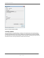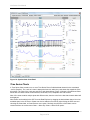
1
VivoSense User Manual – Core Module VivoSense Version 2.3 Vivonoetics - San Diego Office 3231 Huerfano Court, San Diego, CA, 92117-3630 Tel. (858) 876-8486, Fax. (248) 692-0980 Email: [email protected]; Web: www.vivonoetics.com VivoSense Core Manual Cautions and disclaimer VivoSense software is not a medical diagnostic tool and is for research and investigational purposes only and is not intended to be, or to replace, medical advice or review by a physician. Copyright Notice Copyright © 2012 Vivonoetics. All rights reserved. User Documentation VivoSense Core Page 2 of 82 VivoSense Core Manual Table of Contents 1. Introduction ............................................................................................................. 5 1.1. Key Features ................................................................................................................................... 5 1.2. Minimum System Requirements ..................................................................................................... 5 2. Installation .............................................................................................................. 6 2.1. License Management ...................................................................................................................... 6 2.2. Modules ........................................................................................................................................... 9 2.3. Updates ........................................................................................................................................... 9 3. Importing Data with Import Modules ..................................................................... 13 3.1. Supported Hardware ..................................................................................................................... 13 3.2. Importing data ............................................................................................................................... 13 4. VivoSense Files (.vsn) .......................................................................................... 15 4.1. Opening and Saving .vsn Files ..................................................................................................... 15 4.2. Multiple Sessions .......................................................................................................................... 15 4.3. Session Properties ........................................................................................................................ 15 4.4. Launching VivoSense ................................................................................................................... 16 4.5. Working environment (Main Window) ........................................................................................... 16 4.6. Data Explorer and Layouts ........................................................................................................... 22 4.7. Properties ...................................................................................................................................... 24 4.8. Annotation Manager ...................................................................................................................... 25 4.9. Export Manager ............................................................................................................................. 26 4.10. Synchronized Chart Panel (SCP) .............................................................................................. 27 4.11. Preferences ............................................................................................................................... 41 4.12. Annotations................................................................................................................................ 42 4.13. Engineering Toolbox Forms ...................................................................................................... 44 5. Data Processing ................................................................................................... 46 5.1. Data Channel Types ..................................................................................................................... 46 5.2. Channel Parameters ..................................................................................................................... 49 5.3. Parameter Templates.................................................................................................................... 49 6. Device Sensor Data Channels .............................................................................. 51 6.1. Accelerometer Data Channels ...................................................................................................... 51 6.2. Electrocardiogram (ECG) Data Channels ..................................................................................... 52 User Documentation VivoSense Core Page 3 of 82 VivoSense Core Manual 6.3. GSR Data Channels...................................................................................................................... 53 6.4. Pulse Oximeter Data Channels ..................................................................................................... 53 6.5. Respiration Data Channels ........................................................................................................... 53 6.6. Electroencephalography (EEG) Data Channels ........................................................................... 58 6.7. Electromyography (EMG) Data Channels..................................................................................... 59 6.8. Spirometer Channels .................................................................................................................... 59 7. Exporting Data ...................................................................................................... 61 7.1. Defining Export Configurations ..................................................................................................... 61 7.2. Export File Name Conventions ..................................................................................................... 62 7.3. Export .vsn subset......................................................................................................................... 63 7.4. Export Data ................................................................................................................................... 63 7.5. Export Data By Annotation ............................................................................................................ 64 7.6. Export Statistics ............................................................................................................................ 64 7.7. Export Statistics by Annotation ..................................................................................................... 66 7.8. Export Annotations ........................................................................................................................ 66 7.9. Default Export Configurations ....................................................................................................... 67 8. Module Layouts .................................................................................................... 68 8.1. Import Module Specific Layouts .................................................................................................... 68 8.2. General Description ...................................................................................................................... 68 9. Synchronizing Session Data ................................................................................. 70 9.1. Synchronizing Session Start Time ................................................................................................ 70 9.2. Synchronizing Session Cursor Time ............................................................................................. 71 10. Importing Generic Physiological Data Files .......................................................... 72 10.1. Importing CSV and Excel Files .................................................................................................. 72 10.2. Importing European Data Format (EDF) Files .......................................................................... 78 11. Getting Started with VivoSense Video .................................................................. 79 12. Appendix A – Glossary of Terms .......................................................................... 80 13. Appendix B – Hot Keys ......................................................................................... 82 User Documentation VivoSense Core Page 4 of 82 VivoSense Core Manual 1. Introduction This is the user manual for VivoSense’s Core module. Separate user manuals exist for the various import and analysis modules supported by VivoSense software. Chapters 1 and 2 are a brief introduction to VivoSense software and its installation. Chapter 3 describes the concept of import modules and how they support various types of hardware. Chapter 4 discusses the VivoSense file format. Chapter Error! Reference source not found. details the VivoSense environment and Chapter 5 describes the various types of data channels and how they are processed. Chapter 6 lists all available sensors and their respective channels. Chapters 7 and 8 focus on how to export data and use Layouts to create and manage various views of the data. Chapter 10 deals with synchronizing data to external references. Chapter 11 describes importing generic physiological data from non-sensor specific files. The Glossary section in Appendix A provides definitions of terminology that appear in this user manual. Appendix B lists the short-cut keys used in VivoSense. 1.1. Key Features VivoSense is an intuitive, fully customizable visualization and discovery tool that enhances post-processing of data from physiological monitoring sensor platforms. Data can be imported from a variety of devices via import modules Data is processed into VivoSense’s standard data channel architecture Data channels can be visualized in charts capable of displaying and organizing large data-sets. Common processing parameters can be adjusted by the user for derived data channels. Users can create customized selections of charts and define view preferences for a particular analysis. These chart selections can be saved as VivoSense “Layouts”. Users can annotate data channels with notes & comments along the time-series for quick retrieval and review. Data can be exported to text files. Custom, reusable export configurations can be created for convenient re-use. 1.2. Minimum System Requirements The minimum system requirements to run VivoSense are: Operating System: Microsoft Windows XP w/SP2, or later operating system. Processor: 1 gigahertz (GHz) processor or higher Memory: 1 gigabyte of RAM or higher Hard disk: 1.0 gigabyte (GB) Display: 1024x768 or higher resolution monitor User Documentation VivoSense Core Page 5 of 82 VivoSense Core Manual 2. Installation VivoSense software is provided as a downloadable installer. To run the installation program double-click on the installer and follow the on-screen instructions. After installing VivoSense, you will need to provide the required license information and register the system as described in the following sections. 2.1. License Management VivoSense licensing mechanism allows for provisional, time-based or permanent licensing. Trial versions of the software typically expire after a certain number of days. If you purchase VivoSense, you will normally receive a permanent license after registering the software. First time use Your VivoSense license must be configured on your system upon first-time-use by installing a valid license file (*.v2c). If your system does not have a valid license, VivoSense will prompt you with the dialog shown in Figure 1. Figure 1. VivoSense Licensing dialog If you have just purchased VivoSense, you will receive a temporary license file that needs to be installed first. You will then have seven days to register the software before you can receive the final license file from Vivonoetics. If you have a trial license, install it upon initial startup to unlock VivoSense for the duration of your evaluation period. License Manager Having installed the software and the initial license, you can register the product or install license files from the License Manager which is accessible from the VivoSense Help menu (Figure 2).The License Manager also shows the status of the various VivoSense modules. User Documentation VivoSense Core Page 6 of 82 VivoSense Core Manual Figure 2. License Manager Installing License File (*.v2c) A license file can be installed from the VivoSense Licensing dialog, or from the License Manager available from the help menu of VivoSense. Clicking the Install License File button on either of these dialogs will allow you to browse for and install a license file as shown in Figure 3. User Documentation VivoSense Core Page 7 of 82 VivoSense Core Manual Figure 3. License File Installation Registering VivoSense To receive a permanent VivoSense license following purchase of a license, you will need to register the product by submitting the information shown on the Customer Registration dialog (Figure 4). User Documentation VivoSense Core Page 8 of 82 VivoSense Core Manual Figure 4. Customer Registration After your registration has been received, Vivonoetics will send you a full license that can be installed through the License Manager. This will convert your trial version of VivoSense into a fully functional version, with all of the features you purchased. 2.2. Modules VivoSense is a flexible platform that can be enhanced by various types of add-on “modules” that provide extra functionality. If you purchase additional modules for VivoSense, you will receive license files for those modules. These modules can be installed using the License Manager as described in the previous sections. 2.3. Updates An upgrade license is available which unlocks VivoSense's ability to continually keep itself up to date with the latest features and enhancements. If this feature is present, VivoSense will automatically check for updates once upon startup, or at any time the Update Manager is launched from the Help menu. Checking for Updates After the Update Manager has been launched, it will determine if updates are ready to be downloaded. If your copy of VivoSense is current, then the Update Manager will inform you that VivoSense is up to date. (Figure 5) User Documentation VivoSense Core Page 9 of 82 VivoSense Core Manual Figure 5. VivoSense Update Manager dialog If an update is available, VivoSense will display information about the update and allow you to either ignore it, or download it. (Figure 6) After downloading, you then have to option to immediately install the update, or if it is more convenient, defer the installation until a later time. User Documentation VivoSense Core Page 10 of 82 VivoSense Core Manual Figure 6. VivoSense Update available Installing Updates Upon pressing install in the Update Manager, VivoSense will automatically ask for the elevated privileges necessary to perform the update. Under Vista or Windows 7, you will be prompted for a simple authorization (or administrator password if you are running as a standard user), whereas if you are running as a standard user in Windows XP, the 'Run As' dialog will appear. (Figure 7) Select the 'The following user' option, have an administrator enter the correct login information, and then click the 'OK' button. User Documentation VivoSense Core Page 11 of 82 VivoSense Core Manual Figure 7. Run As dialog VivoSense will be closed (after prompting to save any open data files), and the update dialog will be launched. After finishing, the update dialog will inform the user of the success or failure of the update process, and then re-launch. User Documentation VivoSense Core Page 12 of 82 VivoSense Core Manual 3. Importing Data with Import Modules VivoSense import modules provide access to data from a variety of hardware devices and generic import files. The import module imports data recorded or generated by the hardware as “raw” data. Import modules may also derive additional data channels specific to the supported sensor data that are not included in the core module. 3.1. Supported Hardware Some devices store information on memory cards, some provide access via USB ports, while others allows for wireless download of information via Bluetooth. The hardware documentation will explain how to retrieve a data file from the hardware onto the PC. Once the hardware data file is on the PC it may be imported into VivoSense. Correctly formatted ASCII files may also imported see Chapter 10. 3.2. Importing data After installing an import module for a certain type of hardware, the VivoSense File –> Import menu will include commands to import the data from that particular hardware. After importing data, VivoSense Data Explorer will show a top level node named “Raw” that provides access to the (raw) data imported from the device. VivoSense will also generate a standardized set of data channels for use in the VivoSense analysis. Since each device might provide a different set of sensor measurements, there might be some variation in what types of data channels are available after the import. The Data Explorer lists the nodes in alphabetic order. The Data Explorer will be discussed further in Chapter 4.6. Imported .vsn File Location Imported raw data and all the channels generated by VivoSense can be saved to a hardware independent VivoSense file with extension “.vsn“. The default location where these files are stored can be defined in the VivoSense Preferences dialog (Chapter 4.11). If the file is not saved manually via the File menu, VivoSense will provide the option to save the file to the default location when you exit the program. Use the File -> Save As menu command to save a particular file to an alternate location. Please note that you cannot import the same raw data file twice during the same VivoSense session until you have saved and closed the associated .vsn file. IMPORTANT: importing a file is different from opening a previously imported file. In general, a session will only be imported once. Any subsequent viewing or editing of the session should be done by opening the resulting .vsn file. The import file will never be saved, written or otherwise edited by VivoSense and a reimport of a file will not reflect any work done during a previous import. File Name Conventions In general, VivoSense will suggest a default .vsn file name based on the name of the import file, the hardware used, and an index if the file already exists: [HardwareInfo].[ImportedSessionName].[ImportedFileExt][Index].vsn User Documentation VivoSense Core Page 13 of 82 VivoSense Core Manual Please note that the above naming convention may be hardware dependent. Refer to the manual corresponding to the specific import module for more details. The following is the detailed explanation for each part of the file name: HardwareInfo is the optional hardware info prefix. For example, this may be a serial number or subject ID. Refer to your import module documentation for details. ImportedSessionName is the name of the file or session that was imported. ImportedFileExt is the extension of the file that was imported. Index is the optional index of the vsn file on disk. If the file name already exists on disk in the Data folder, then the index field starts at 000 and increments until a unique file name is found. User Documentation VivoSense Core Page 14 of 82 VivoSense Core Manual 4. VivoSense Files (.vsn) VivoSense stores all the data corresponding to an individual session in a single file denoted with the extension “.vsn”. This file format is proprietary and uses compression and encryption. It contains all the raw data imported from the device, as well as the results of any user interaction such as annotations, calibration, tuning of algorithm parameters and data editing. In general, no derived waveforms, markings, measures, or trends are stored in the .vsn file. Instead they are recalculated every time the file is opened. 4.1. Opening and Saving .vsn Files VivoSense files are opened via the File -> Open menu command. After opening a .vsn file, it will be identified as a session-node in the Data Explorer window, and also be represented with a dedicated Synchronized Chart Panel for data visualization. The Data Explorer and the Synchronized Chart Panel are discussed in greater detail in Chapter 4.5. Alternatively, a .vsn file may be opened by dragging it from any Windows Explorer and dropping it on VivoSense’s Data Explorer, or simply double-clicking the .vsn file from any Windows Explorer. The file can be saved back to disk with the File -> Save menu command. If you exit VivoSense after making changes to any Channel Properties or other settings associated with the file, you will be prompted to save your changes before exiting the program. 4.2. Multiple Sessions VivoSense can open and manage multiple .vsn files simultaneously. Each file is represented by a top-level session-node in the VivoSense Data Explorer and also by a dedicated Synchronized Chart Panel to visualize the data in the file. The Data Explorer and the Synchronized Chart Panel are discussed in greater detail in Chapter 4.5. 4.3. Session Properties Information about a session can be accessed in the properties window when first opening a .vsn file, by clicking on the session-node in the data explorer, or from the Session ->Properties ->Show menu item. Many of these properties are read-only, but there are some user editable fields. Session Start Time Session Start Time is the start date and time of the session. Adjusting this property will shift all the data and annotations in absolute time. This does not truncate or expand the duration of the session. Session Time Zone Session Time Zone is the time zone that the data was recorded in. Editing this property allows you to set the time zone if it is different than the one that the data was imported in. Subject ID The data analyst or researcher may enter text unique to the session, such as randomization number or subject name in this field. To modify this property edit it directly in the property window. User Documentation VivoSense Core Page 15 of 82 VivoSense Core Manual User Session Properties The user may also add, remove, or edit their own properties for a session from the Session ->Properties menu item. Here you may enter an optional Category and/or Description of the Property in addition to the Name and Value. The Category defines how the properties are grouped in the Properties Window. The Description explains the property in the bottom of the Properties Window when a property is selected. 4.4. Launching VivoSense VivoSense can be launched from the Windows Start-menu, under the Vivonoetics folder. By default, the program is installed to one of the following locations: C:\Program Files\Vivonoetics\VivoSense\VivoSense.exe (On 32-bit Windows) C:\Program Files (x86)\Vivonoetics\VivoSense\VivoSense.exe (On 64-bit Windows) 4.5. Working environment (Main Window) This section describes features specific to the VivoSense Core in a typical installation. You may see more or less features depending on which modules your installation is licensed for. If you see a button or menu option not explained here, refer to the user manual for the specific module. The VivoSense environment is composed of several elements: the Menu Bar, Standard Toolbar, various SubWindows that are docked to the left, bottom and right sides, as well as the central area for viewing and visualizing data. When data is imported, or when the user opens one or more VivoSense files, the central area will be populated by one Synchronized Chart Panel (SCP) for each open file. User Documentation VivoSense Core Page 16 of 82 VivoSense Core Manual Figure 8. VivoSense Working Environment The following sections describe the various user interface elements. Menu Bar The main Menu Bar provides access to commands and settings available in VivoSense. The top-level menu items include: File, Session, View, Tools, Windows and Help. User Documentation VivoSense Core Page 17 of 82 VivoSense Core Manual Figure 9. Main Menu The following is a listing of sub-menu items it a typical installation (You may see more or less options based on which modules your license enables, and what the active session is): File Menu The file menu commands are summarized in the following table: File Menu Items Feature description Import Hardware File Import data into VivoSense from supported physiological sensor systems. The available type of imports depends on what import modules are present on the system. Import … Short cut to import data from the most recently selected file format. Open .vsn File Open an existing VivoSense file (.vsn) Close Close the selected session file (.vsn) Close All But This One Close all session files except the selected one Save Save the selected session File (.vsn) Save As Save the selected session file to another file name Recent Files Shows a list of recent session files (.vsn) User Documentation VivoSense Core Page 18 of 82 VivoSense Core Manual File Menu Items Feature description Clear Recent File List Clears the list or recent session files Print If a printable object is selected, print it Print Preview Preview how the printable object will look as printed Page Setup Configure page margins and other printing preferences Exit Exit VivoSense, with option to save modified .vsn files Session Menu (only visible when a file is open) The Session menu commands are summarized in the following table: Session Menu Items Feature description Annotations Manipulates annotations, refer to VivoSense - Batch Processing Module File-Save File Save the selected session File (.vsn) Import-Event Log Imports an excel event log as annoations Export-Data Export session-data to text file Export-Statistics Export statistics for the Session to text file Export-Annotations Export session annotations to text file Export-.vsn Subset Extract data within specific interval from session to a new .vsn file Properties Add, edit, remove, or show Session Properties Template-Save Save channel properties to an existing template Template-Save as Save channel properties to a new template Template-Load Load channel properties from an existing template Set Start Time Synchronize the session start time with a new date and new start time View Menu The View Menu commands are summarized in the following table: View Menu Items Shortcut Feature description Data Explorer F3 Show the Data Explorer Sub-Window. The Data Explorer Sub-window includes display of all Session objects, their Data Channels and the Layout Explorer window Property Window F4 Show the Properties Sub-Window. The Properties window shows the properties of the selected object Export Manager F6 Show the Export Manager Sub-Window. The Export Manager lets you define and save named export Configurations for use by the Session-Export-Data command Annotation Manager F7 Show the Annotation Manager Sub-Window, which lists all annotations for the active session (.vsn) User Documentation VivoSense Core Page 19 of 82 VivoSense Core Manual Large Icons Toggle between normal and large Icons Tool Bar Toggle the Tool Bar on/off Refresh F5 Refresh view Tools Menu The Tools Menu commands are summarized in the following table: Tools Menu Items Feature description Preferences Show the VivoSense Preferences Window, which lets you define the preferred location of your files Window This Window Menu shows shortcuts to any open .vsn files (Session) Window Menu Items Feature description … .vsn The Windows Menu contains shortcuts to any open Session documents (.vsn files) Help The Help Menu commands are summarized in the following table: Help Menu Items Feature description About VivoSense Show details about the current version of VivoSense License Manager Show the License manager window Update Manager Show the Update Manager window Documentation Shows a menu of VivoSense documentation including this User Manual and the User Manual for installed modules Toolbar The Toolbar provides one-click access to common functionalities and commands in VivoSense. To show/hide the Tool Bar, use the View – Tool Bar menu option. Figure 10. Toolbar The available Toolbar commands are summarized in the following table: Tool Bar Command Feature description User Documentation VivoSense Core Page 20 of 82 VivoSense Core Manual Tool Bar Command Feature description Open Open an existing VivoSense file (.vsn) Save Save the selected session file (.vsn) Save As Save the selected session file to another file name Print Preview Generate preview of the active layout Print Print active layout Data Explorer Shows the data explorer sub-window Property Window Shows the properties sub-window Annotation Manager Shows the annotation manager sub-window Export Manager Shows the export manager sub-window Sub-Windows VivoSense consists of a main window and several sub-windows which can be arranged by the user. Some of the sub-windows can be docked along each perimeter of the main window (i.e. top, bottom, left or right), or can be left floating, while other sub-windows may only reside in certain locations. To move a sub-window, click and drag the caption bar and move the window to the desired destination. Areas where the window can be docked are indicated as rectangular “drag & drop areas”, as the window is moved around within the main VivoSense window. The Sub-Windows include: Data Explorer Properties Annotation Manager Export Manager Synchronized Chart Panel (SCP) These are discussed in the following sections. User Documentation VivoSense Core Page 21 of 82 VivoSense Core Manual 4.6. Data Explorer and Layouts Data Explorer – Sessions and Channels The Data Explorer (Figure 11) shows the content of one or more .vsn files, or “Sessions”. The Data Explorer provides access to all the available categories of data channels in the file. The available data channels depend on the hardware used to record the data and the licensed analysis modules. Figure 11. Data Explorer Sub-window – Top section Recursive View By default, only the channels from the currently selected Sessions folder will be displayed. The Data Explorer may be customized to show channels from the currently selected Sessions folder and all its subfolders by right-clicking and selecting Recursive. Detail View By default, only the channel names are shown in the Channel list. The Data Explorer may further be customized to show details of each channel by right-clicking and selecting Details. The channels may be sorted by clicking the header of the detail column. The Data Explorer also contains the Layout Manager window, normally shown below the Sessions and Channels panels. User Documentation VivoSense Core Page 22 of 82 VivoSense Core Manual Data Explorer - Layouts The layout Explorer window makes it easy to manage various Chart Layouts for use in the Synchronized Chart panel for the associated “Session”, or .vsn file. Pre-configured chart layouts for each import module are defined under the Common folder. The user can create custom Chart Layouts in the User folder. Figure 12. Layouts Sub-window (Bottom section of Data Explorer) The Layouts window shows 3 types of Layouts; User, Modules and Active. The User layouts are managed by the user of VivoSense. New Layouts can be added, and Layouts can be organized in sub-folders. The content of the modules layout node depends on the licensed import and Analysis modules, and provides customized set of Layouts suited to the particular module. See Chapter 8 for more details regarding the module Layout folder. The Active layout node shows the Layouts used by each Session (file) open in VivoSense at any point in time. Saving User Layouts To save a particular Layout, view the Synchronized Chart Panel for the session of interest. Then Add the Charts and Plots as desired. When complete, right-click on any of the Charts and use the Layout -> Save context menu command. You will be able to either select a Layout Folder in order to generate a new Layout within that folder, or you can click on a particular Layout file to override it with the current Layout configuration. Loading User Layouts You can apply, or load a particular Layout to your selected Synchronized Chart panel by double-clicking on a Layout in the Layouts Sub-window. You can also do the same from the Synchronized Chart Panels context menu, via the Layouts -> Load menu command. Empty Layout Included is an empty layout that may be used to clear the synchronized chart panel so that a user may construct a new layout. This is more convenient than removing all the charts in an existing layout on a chart by chart basis. User Documentation VivoSense Core Page 23 of 82 VivoSense Core Manual 4.7. Properties The Properties sub-window (Figure 13) provides access to property data for the selected object. Different objects may have different properties, some of which the user can modify and some which they cannot. The most common objects to modify via the Properties window are Data Channels, Charts, Plots and Annotations. To show the properties of these entities, first make the Properties Window visible via the View –> Property Window menu command, or press F4. Then select the appropriate object. The following is a list of typical usage of the property window for the most common objects: Data Channel properties can be viewed and a subset of these may be edited by the user. To display these properties, click on the channel in the Data Explorer, or click on the Name of a Chart Legend (i.e. the name of the Data Channel). Examples of such user editable parameters are the trend window length of Trend Channels or the Lockout Period of the R-wave picker. Trend Channels are described in greater details in Chapter 5.1 and a description of all other editable Data Channel parameters is presented in Chapter 5. Note: any changes to the Channel parameters persist in the corresponding .vsn file. Chart Properties are used to customize how the Chart is visualized and also to edit the Chart’s caption. To show the Chart properties, click within the chart area. Charts are described in greater details in Chapter 4.10. Plot Properties are used to customize how each channel in a Chart is visualized. To show the Plot properties, click on the associated Legend symbol in the Chart. Plots are described in greater detail in Chapter 4.10. Annotation properties can be displayed, and the Annotation description (Note and Name) may be edited for User Annotations. Other annotation types are read-only. See Chapter 4.8 for more details regarding Annotations. Session related information may be found by selecting the corresponding session in the Data Explorer. User Documentation VivoSense Core Page 24 of 82 VivoSense Core Manual Figure 13. Properties Sub-window Editing properties of multiple objects The Property window may also be used to manipulate properties of multiple objects of the same type. An example of this would be to configure multiple Trend Channels to use the same Trend parameters. To do this, make sure the Property window is shown, and then select multiple Trend Data Channels in the Data Explorer window using standard windows CTRL and/or SHIFT keys. The Properties window will show multiple trend channels in its caption. Now make changes to the Trend properties such as Window Width and/or overlap. The changes will apply to all the selected Trend Channels. 4.8. Annotation Manager The Annotation Manager shows all Annotations associated with the given session. One or more annotations can be removed by selecting the row(s) and using the delete key, or by using the context menu’s Remove command (right-click within the Annotation Manager to bring up the context menu). Likewise, annotations can be hidden or shown by clicking the ‘Visible’ checkbox next to any annotation, or by right clicking and choosing Hide or Show from the context menu. By selecting an annotation in the Annotation Manager, the Synchronized Chart Panel will center on the timeperiod of the annotation. The up/down key can be used within the Annotation Manager to quickly move between annotations while the Synchronized Chart Panel focus on the selected one. The annotations may be sorted by clicking on the column header. User Documentation VivoSense Core Page 25 of 82 VivoSense Core Manual Figure 14. Annotation Manager Sub-window The “Source” column in the Annotation Manager indicates the origin of the annotation. There are currently three sources of annotations; User, Hardware and Algorithm. User annotations are manually added by the user. Hardware Annotations are events that are transferred over during the hardware import. Algorithm annotations are the indirect result of a user invoked VivoSense command that leads to a manipulation of the data, such as calibration, artifact editing, or interpolation. These types of annotations cannot be edited directly by the user. They may only be changed by undoing the underlying operation. Whether and how this may be completed is specific to the type of user command that led to its creation. 4.9. Export Manager The Export Manager sub-window (Figure 15) lets the user define standardized “Export Configurations” for use when exporting data. Each module also comes with some pre-defined Export Configurations. By pre-defining standard Export Configurations, it becomes easier to export data in consistent formats, from one or more sessions. Chapter 7 includes description of how to use the Export Manager to create Export Configurations and how to use those Configurations when exporting data. Figure 15. Export Manager Sub-window User Documentation VivoSense Core Page 26 of 82 VivoSense Core Manual 4.10. Synchronized Chart Panel (SCP) The Synchronized Chart Panel (SCP), shown in Figure 16, is a collection of time-synchronized Charts showing data from the associated Session file (.vsn). The SCP also contains tools to navigate in time, change the time-scale, and remove or edit annotations related to the Session Data. The SCP can be quickly re-configured to show different representations of charts from the Layout Window (part of the Data Explorer sub-window). Only one SCP exists for each .vsn file, but use of Layouts allows for quickly loading pre-configured Chart selections into the SCP. The top right of the SCP contains status information about the available data in the session file, such as the Session Start Time and the Session Duration. The Top left of the SCP allows for defining the time-range to be shown in the charts (Numeric input of the Start Time and a combo-box for defining the desired Duration of the data.) The bottom of the SCP contains the SCP status bar, which shows a variety of useful status-information about the SCP, such as cursor time-values as well as the numeric value of the various plot parameters for the chart below the cursor. User Documentation VivoSense Core Page 27 of 82 VivoSense Core Manual Figure 16. Synchronized Chart Panel Time Series Charts A Time Series Chart contains one or more Time Series Plots of individual data channels in the associated .vsn file (Session). The x-axis of a chart is always the time-axis, while the y-axis shows the magnitude of the plot values. The units of the x-axis are specific to each data channel. Figure 16 shows a Synchronized Chart Panel with five charts named Accelerometers, Heart Rate, ECG, RespRate and Tidal Volume. Note: If the chart contains multiple plots with different units, then the units for the last data channel added will be displayed. New Charts can be added to the SCP from the Data Explorer by dragging the desired data channel icon into available space in the SCP area. Charts can also be added or removed by right-clicking the SCP area and choosing the Chart-New, or Chart-Remove menu option. Similarly, the sequence of the Charts can be customized from the context menu Chart -> Move Up / Chart -> Move Down option. User Documentation VivoSense Core Page 28 of 82 VivoSense Core Manual Plots are discussed in the following section, which also includes information on how to add and remove these from the Chart as well as how to change their appearance. Time Series Plots A Time Series Plot is a visualization of a single Data Channel within a given Chart. For each Plot added to a chart, there is a legend symbol and an associated text label showing the name of the Data Channel, as shown in Figure 17. To add a new plot to a chart, drag and drop a Data Channel from the Data Explorer onto the Chart. To remove a plot from a chart, then right-click the associated legend to bring up the context menu, and select the Remove command. Important: There are useful shortcuts to edit both the plot and data channel properties. To modify the Plot properties (Legends) or the Data Channel properties of a plot, make sure the Properties window is visible, and do one of the following: Click on the Legend Symbol to show the Plot Properties Click on the Legend Text (Data Channel Label) to show the Data Channel properties Another option is to right-click on any of the two to bring up the legend context menu, giving options to Remove the plot, or show the Plot Properties or the Channel Properties. Figure 17. Legend Symbol and Text (Data Channel Label) for a Chart with 2 Plots Plot Properties (Legends) The Plot properties provides control over the line and point color, style, width/size while also providing access to alternate ways of visualizing the plot, such as “Line Staircase” mode and “Spike” visualization. User Documentation VivoSense Core Page 29 of 82 VivoSense Core Manual Figure 18. Plot Properties (Legends) Most of the Plot Properties are self-explanatory, and include settings for color, style, size/width for lines and points. To turn points or lines on/off, use their Style property and set the Point Style to None, or Line Style to None. Lines can be visualized using the Staircase mode, where the value of the plot is maintained between points instead of using linearly interpolating the values. This results in a “staircase” appearance of the plot. To use this feature, set the Line Staircase property to true. To draw vertical lines between the x-axis and each data point, simply set the Spike property to True. As with the Lines, the Spike Color, Style, and Width properties may all be customized. To leave only the spikes showing, turn off the Points or the Lines by setting their Style to None. Plots can be modified to show Y-Axis value on the left or the right or to automatically scale the data in the plot to an invisible Y-axis. By assigning different Y-axes (left and right) to overlaid data on a chart, it is possible to view a chart with 2 Y-axes. Use the Y-Axis plot properties drop down menu to make a selection. The side on which the Y-Axis is displayed on a plot can be identified by the check marks displayed on the plot properties legend icon. Tick marks on the left identify that the Y-Axis values are displayed on the left of the plot. Tick marks on the right identify that the Y-Axis values are displayed on the right of the plot. If the Y-Axis Auto setting is chosen, no tick marks will display. See Figure 17 The Fill plot property fills the plot with the fill color from the data points to the base value (generally 0). User Documentation VivoSense Core Page 30 of 82 VivoSense Core Manual Channel Properties – As they apply to a Plot Some Data Channels are calculated “on the fly” based on the Channel Properties. In the context of a Plot, the Trend Data Channels are good examples of this. For convenience, the Trend Parameters may be modified for the Trend Data Channel by clicking the Legend Text of a given Plot (as described previously). Phase Charts A Phase Chart contains a single Phase Plot of multiple data channels in the session: the Y Channel, X Channel, and optionally a Trigger Channel. The Y Channel is plotted on the y-axis against the X-Channel on the x-axis. The units of the axes are specific to each data channel. Arrows along the plot reference the direction forward in time. Figure 19 shows a Synchronized Chart Panel with two Time Series Charts (Compartments and Combined), and two Phase Charts (Konno-Mead and Flow-Volume). New Phase Charts can be added by right-clicking on the SCP area and choosing Chart->New->Phase. The user will be prompted to select the Y Channel, X Channel, and optional Trigger Channel when the Phase Chart is added. Phase Plots are discussed in the following section. Figure 19. Synchronized Chart Panel With Phase Charts User Documentation VivoSense Core Page 31 of 82 VivoSense Core Manual Trigger Channel The Trigger Channel is optional (but also must be set when the Phase Chart is created). It is the channel that triggers the range of data shown on the Phase Plot. When no Trigger Channel is set, then Phase Chart will plot the data within the time range displayed in the SCP. When a Trigger Channel is specified, then the range of data plotted is specified by the crosshair cursor position on the SCP, Trigger Channel, Trigger Start, and Trigger Count. For example to plot Vt vs dVt (Flow-Volume) for three breaths from the crosshair cursor, set the Trigger Channel to Resp Rate, Trigger Count to 3, and Trigger Offset to 0. To plot the three breaths following those, set Trigger Count to 3 and Trigger Offset to 3. (See Figure 20). Figure 20. Selecting the Trigger Channel and Settings The Trigger Count and Trigger offset may be modified in the phase plot properties (See Figure 22). Phase Plots A Phase Plot is a visualization of one Data Channel versus another Data Channel within a given Phase Chart. For each Phase Plot added to a chart, there is a legend symbol. To modify the Phase Plot properties, make sure the Properties window is visible, and click on the Legend Symbol. Phase Chart Properties To modify the Phase Chart properties, make sure the Properties window is visible, and click on the Phase Plot. The Phase Chart Properties provides control over the colors and name of the chart, as well as how the data is scaled in the Auto Scale property. Set Auto Scale to XYAxis_Symmetric to show the entire data set, and have equal range. This is useful if the shape of the curve (circular vs elliptical) is important. Set Auto Scale to XYAxis to have each axis scale independently. User Documentation VivoSense Core Page 32 of 82 VivoSense Core Manual Figure 21. Phase Chart Properties Phase Plot Properties The Phase Plot properties provides control over the line and point color, style, width/size while also providing access to alternate ways of visualizing the plot, such as “Line Staircase” mode and “Spike” visualization. User Documentation VivoSense Core Page 33 of 82 VivoSense Core Manual Figure 22. Phase Plot Properties Other Phase Plot Properties include settings for color, style and size/width for lines and points. To turn points or lines on/off, use their Style property and set the Point Style to None, or Line Style to None. To turn directional arrows off, set the Arrow Count to 0. Lines can be visualized using the Staircase mode, where the value of the plot is maintained between points instead of using linearly interpolating the values. This results in a “staircase” appearance of the plot. To use this feature, set the Line Staircase property to true. (See Figure 22). User Documentation VivoSense Core Page 34 of 82 VivoSense Core Manual Bland-Altman Chart A Bland-Altman Chart contains a single Bland-Altman Plot. To create a Bland-Altman Chart, right click on a chart on the SCP and select Chart->New->Bland-Altman. You will be prompted to select the two data channels to compare. Bland-Altman Plot A Bland-Altman Plot is the difference versus the average of two similar Data Channels. It visualizes the agreement of two channels and may be used to compare two measures acquired with different sensors or algorithms, or compare a gold standard data channel to a new data channel. The Limits of Agreement are drawn at +- 1.96 Standard Deviations, and may be edited through the plot properties. Figure 23. Bland-Altman Chart comparing RR intervals acquired from different ECG electrodes. User Documentation VivoSense Core Page 35 of 82 VivoSense Core Manual Regression Fit Chart A Regression Fit Chart contains a single Regression Fit Plot. To create a Regression Fit Chart, right click on a chart on the SCP and select Chart->New->Regression Fit. You will be prompted to select channels for the Y-axis and the X-axis. Regression Fit Plot A Regression Fit Plot contains a scatter plot of one Data Channel versus another Data Channel, and then performs a Least Squared (R2) Linear fit, and plots this as a straight line. This is useful for visualizing the correlation between two Data Channels. Figure 24. Regression Fit Plot showing correlation between Trended Respiration Rate and Trended Heart Rate. User Documentation VivoSense Core Page 36 of 82 VivoSense Core Manual Power Spectral Density Chart A Power Spectral Density Chart contains a single Power Spectral Density Plot. To create a Power Spectral Density Chart, right click on a chart on the SCP and select Chart->New->Power Spectral Density. You will be prompted to select a Data Channel. Power Spectral Density Plot Power Spectral Density (PSD) Plots provide visualization of the frequency components of a Data Channel, by plotting the Power on the y-axis against frequency on the x-axis. Frequency bands, represented by color coded Shading may optionally be specified. The Shading ranges and colors, as well as the PSD Settings may be edited through the plot properties. . Figure 25. PSD Plot of Vt, with a Shading region of the frequencies between 0.2 and 0.25 Hz. This range corresponds to 3 to 4 seconds/breath or 15 to 20 breaths/minute. User Documentation VivoSense Core Page 37 of 82 VivoSense Core Manual Histogram Chart A Histogram Chart contains a single Histogram Plot. To create a Histogram Chart, right click on a chart on the SCP and select Chart->New->Histogram. You will be prompted to select a Data Channel. Histogram Plot Histogram Plots provide visualization of the distribution of samples of a Data Channel, by plotting the count of samples that fall within a particular range (called a bin) on the y-axis against the bin on the x-axis. The Bin Count may be specified in the Plot Properties. The histogram is computed differently depending on the Bin Style property. Auto The minimum and maximum data points are found, and the bins are distributed evenly across this range. Manual The user enters the Minimum and Maximum in the properties window. The bins are distributed evenly across this range. Standard Deviations The width of each bin is set to the Standard Deviation of the data. The bins are centered around the Mean of the data. For odd number of bins, the mean will be in the center of the center bin. For even number of bins, the mean will be between the two center bins. Figure 26. Histogram Chart showing distribution of Respiration Rate. User Documentation VivoSense Core Page 38 of 82 VivoSense Core Manual SCP Status bar The Synchronized Chart Panels Status Bar shows pertinent status information on a given session. Figure 27 shows a few samples of what type of information is shown in the status bar. During a file open or import operation, the Status bar shows the progress of the operation While navigating Charts in a Layout, the status bar shows cursor information, such as time and value at the cursor, and also the values of the various plot parameters in the chart below the cursor During range-selection or measurements (during click & drag operations with the mouse on a Chart) the Status bar shows the difference in time (“Time Diff”) between the first click and the current cursor position. It also shows the vertical range (“Cursor Diff”). Some channels may provide more information, for example RAW channels show the number of samples, and Resp Rate shows the number of events (breaths). Figure 27. Status bar - Import a File, Navigating a Chart, and Selecting a Range Navigating the Charts Resizing Charts Each chart may be resized vertically by clicking and dragging the invisible line between each Chart up or down (The Mouse-cursor will appear like a resize-handle when the cursor is at the right location.) Changing Vertical scale The vertical scale of a chart can be configured automatically, or manually adjusted. To enable Automatic vertical scale for a Plot each time the layout (visible) range changes, set the Auto Scale Plot Property to true for the desired Plot. To auto-scale all plots in the Chart for your current layout range, select Center Range from the Chart Context Menu. Clicking on the upper or lower axis label will manually change the range of the vertical axis. Changing Horizontal Scale To change the Horizontal scale, adjust the Total Duration for the SCP, using the combo box at the top edge of the SCP, or Zoom in to the desired window by clicking and dragging a rectangle around the desired set of data. Then select the Zoom Selection command. Double-clicking on a Chart will zoom in 50% and center around the cursor position. Alternatively, use the Up and Down Arrow keyboard shortcuts to adjust the horizontal scale (50% change in scale for each arrow press) User Documentation VivoSense Core Page 39 of 82 VivoSense Core Manual Scrolling in time – Along X-axis Use the scroll bar at the bottom of the SCP to move the layout range forward or backward in time. Alternatively, use the Left and Right Arrow keyboard shortcuts. Cursor Positions While hovering the mouse over the SCP and its charts, the Status Bar will show the following information about the cursor position: Time, Cursor (the vertical position of the cursor), and Values (the Chart’s various plot values at the cursor Time). Cursor Measurements The cursor may also be used to measure a range in time or magnitude. Click on the starting point and drag the cursor towards the end point. The Status Bar will show the time difference and cursor difference between the two positions. When letting go of the left mouse button, the Charts Context Menu will be shown. The Charts Context Menu contains a large number of possible options, some of which take advantage of the selected range. Chart Context Menu The Chart Context Menu commands are summarized in the following table. Some of these menu options are contextual (i.e. they are available depending on whether the user right-clicked a chart, selected a time-range from a chart, and what data channels are associated with the plots for the selected chart) Chart Context Menu Shortcut Feature description Zoom Last Zoom to previous time range Zoom All Zoom to range of available data Zoom Selection Adjust the horizontal range of all Charts in the Synchronized Chart Manager to match the selected time period. (Only available when a range of time is selected) Zoom Annotation Adjust the horizontal range of all Charts in the Synchronized Chart Manager to match the selected annotation. (Only available when a single point is clicked on a chart within an Annotation) Refresh F5 Refresh the Synchronized Charts Center Range Scale Chart vertically so all data within time-range is shown Annotations - Add Add an annotation for the selected time range Engineering Toolbox- * Popups an Engineering Toolbox form with the selected chart type, based on the selected range and channel(s) on the selected chart. Chart - New Add a new chart Chart - Remove Remove the chart below the cursor Chart – Move Up Move the chart below the cursor up Chart – Move Down Move the chart below the cursor down User Documentation VivoSense Core Page 40 of 82 VivoSense Core Manual Chart Context Menu Shortcut Feature description Chart - Properties Show the Charts Properties in the Property window Plots – Add Plot Add a new plot to an existing chart. Plots - *** - Plot Properties Show the Plot Properties of the desired Plot (***) Plots - *** - Channel Properties Show the Channel Properties of the desired Plot (***) Layout - Save Save the current Chart configuration as a new Layout Layout - Load Load a new layout into the Synchronized Chart Panel Properties Show the common Properties of all Charts Export - Data Same as Session-Export Data, but with selected time period Export - Statistics Same as Session-Export Statistics, but with selected time period Export - Annotations Same as Session-Export Annotations, but with selected time period Export – Export .vsn Subset Same as Session-Export .vsn Subset, but with selected time period Set Cursor Time Synchronize the session cursor time with a new date and new start time. Artifact Management – Exclude – Exclude as Artifact For RAW channels only. Marks the selected range as artifact and excludes all RAW and Derived data from further analysis. Artifact Management – Exclude – Remove Exclusion For RAW channels only. Removes the selected exclusion. Artifact Management – Audit For RAW channels only, temporarily shows the data within the artifact exclusion. Layouts and SCP The Layout Window, described in Chapter 4.6 may be used to save and restore the Charts and Plots shown in the SCP. A current Layout may be Saved or one of the Layouts may be Reloaded in the Layout Window of the SCP by right-clicking on a Chart and choosing the Layout -> Save or Layout -> Load context menu command VivoSense also comes with pre-configured Layouts for each module. See Chapter 8 for more information about module Layouts. 4.11. Preferences The Preferences window available from the Tools-Preferences menu command allows the user to modify various default settings. Below is a list of tabs related to the VivoSene Core module (see Figure 28). Additional tabs related to extension modules are described in the corresponding manuals. User Documentation VivoSense Core Page 41 of 82 VivoSense Core Manual Folder Preferences In this tab the user can set the default locations for the various files. VivoSense will look for .vsn files in the Data Folder. The Import Folder is where VivoSense will look for raw data files, and the Export Folder is where exported data will be saved by default. Respiration Preference In this tab the user can set the default parameters related to respiration. The ‘Average Breath Volume’ for a healthy adult is 400 ml. This parameter is used by the initial raw calibration and as the default parameter in the FVC dialog. The ‘Relative Deadspace’ parameterizes the minimum tidal volume required in the identification of a breath while ‘Minimum Flow’ limit is used to identify the beginning and the end of inspiratory/expiratory flow. Additional parameters such as the QDC parameters shown in Figure 28 may be accessible depending on whether a license is available for the corresponding extension module. Figure 28. VivoSense Preferences 4.12. Annotations As described in Section 4.8, VivoSense supports three sources of annotations; User, Hardware and Algorithm. User annotations allow the custom marking and labeling of events of interest. To create a user annotation, left click the mouse at the start time of the event and hold it down. Drag the mouse until the end time of the event and then release the mouse. This creates a pop-up context menu where selecting Annotation->Add will create the desired annotation. See Figure 29. User Documentation VivoSense Core Page 42 of 82 VivoSense Core Manual Figure 29. Creating User Annotations. Annotation Properties The annotation properties provide control over changing the color, transparency, name, notes and visibility associated with annotations. Note that selecting the Visible field in the annotation properties to False will only display the annotation in the annotation manager but not show it in any of the available charts. Moving and Resizing Annotations Following addition of an annotation, it is possible to move or resize the annotation. This is completed using the annotation bar. This is the bar at the top of the SCP that contains the text describing the annotation. The default text is simply ‘User Annotation’. This may be truncated depending on the size of the text and the current level of zoom. User Documentation VivoSense Core Page 43 of 82 VivoSense Core Manual To move an annotation, place the mouse over the annotation in the annotation bar region until the cursor changes to the ‘move’ cursor. Then left click on the bar and drag it to a new location. To resize, place the cursor at the edge of the annotation on the annotation bar until the ‘resize’ appears. Then left click and hold down and stretch or shrink the annotation. cursor Sometimes an annotation may be “hidden” behind another one. To access the hidden annotation, right click on the annotation in front and select Annotation->Send To Back. Importing an Event Log To import an Excel spreadsheet event log as annotations select the Session-> Import-> Event Log menu item. Select the Input File Name and specify the letters of the columns for the different properties in the annotation. Specify the number of rows, if any, after the first row to ignore before importing data. The Color Column is optional. Most common color names are supported along with a light variant, such as Blue, LightBlue, Gray, LightGray, Green, LightGreen, etc. For a complete list refer to any of the Color property drop down editor for an Annotation, or here: http://msdn.microsoft.com/en-us/library/system.drawing.knowncolor.aspx This import requires Excel 2007 or later ODBC drivers installed. If you do not have them installed, they are included in the AccessDatabaseEngine you may download them from here: http://www.microsoft.com/download/en/details.aspx?id=13255 4.13. Engineering Toolbox Forms The Engineering Toolbox Form is a stand-alone popup SCP and Properties window. To display an Engineering Toolbox Form, select a range of interest on a chart containing the channel or channels of interest. The channel from the selected chart will be used on the form. If the form requires more channels you will be prompted for them. User Documentation VivoSense Core Page 44 of 82 VivoSense Core Manual Figure 30. An Engineering Toolbox Form showing a Regression Fit of RR intervals from two different sensors. Once launched, this window is independent of the main form. The properties window is always docked on the right, but may be hidden from the toolbar. You may navigate, edit properties, add and remove charts, and do most other visualization tasks that are available in the SCP. This allows you simultaneously display multiple SCP visualizations of the same session, or quickly pop up a tool, such as a Bland-Altman, Regression Fit, Power Spectral Density, or Histogram Chart. The SCP may be printed from the toolbar. User Documentation VivoSense Core Page 45 of 82 VivoSense Core Manual 5. Data Processing In general, a vsn file only stores the raw data recorded during a session, some session related information and any user input such as annotations or parameter modifications. In addition to being an export and visualization tool for raw data, VivoSense contains many algorithms for deriving useful metrics or indices from basic physiological raw channels (For definition and details on channels see Appendix B). Frequently, the result of an algorithm is available as another data channel referred to as ‘derived channels’ (indicating that the channel is derived from some other channel). The execution of an algorithm is triggered by exporting the derived channel or displaying it inside a chart. 5.1. Data Channel Types VivoSense supports Data Channels of different Types, such as Waveforms, Markings, Measures and general Info channels. These channel types are described in the following sections. Waveforms A Waveform is defined in VivoSense as time-series data sampled at an even sample rate. The data is typically raw sensor information or raw sensor information processed through filtering or signal enhancements. For example Figure 31 shows a Waveform data channel containing ECG measurements sampled at 256 Hz. Figure 31. Waveform sample channel Markings A Markings Data Channel is used to mark points on a Waveform channel and is typically the result of running a processing algorithm on one or more Waveform channels. These Markings are key features or patterns that have physiological significance or that may be used to derive further significant measures. Markings channels are a set of time-value data points at discrete points in time. User Documentation VivoSense Core Page 46 of 82 VivoSense Core Manual Figure 32. -R-Wave Markings channel which mark the peak value of each R-wave in an ECG waveform, shown here on the same chart as the underlying ECG Waveform Measures A measure contains data derived from one or more Waveforms or Markings data channels, but can also contain data sampled from a device (i.e. a Raw data channel). A data point in a Measures data channel has both time and value associated with it, and in contrast to the Waveform, Measures are not necessarily calculated, or sampled, at a constant rate. Some measures are calculated for a given time-range, or between two Markings. If so, the Measure is always time-referenced to the start of the range. An example of this is instantaneous heart rate, which is calculated based on the time between consecutive R-wave Markings. The heart rate value then applies to any point in time between the two R-wave Markings. Other measures are calculated based on a combination of Markings and Waveforms. Respiration Measures are typically derived from markings such as the beginning and end of inhalation, based on the flow and or the peak flow etc. Since the time stamps of these Markings are usually at irregular intervals, the associated Measure-calculations are also irregular in nature. Trends Trends are considered “derived data channels” in that they rely on trend calculations of data in the source channel, and are calculated “on the fly” by VivoSense. Trends are typically available for all data channels containing Measures. Each module provides certain pre-configured Trend definitions for the available Measures. A Trend calculation is calculated using a “moving window” approach, where the data (Measures) within the window is used to calculate a representative trend-value for that time interval. Trend properties The trend properties are initially configured by VivoSense when importing the data, but can be customized by the user, as described in the following sections: Trend Window Width The Trend Window Width is the width of the moving trend window in seconds, i.e. the time duration over which the trend is calculated. The default Trend Window Width is 1 minute. The time associated with each calculation is in the center of the Trend Window User Documentation VivoSense Core Page 47 of 82 VivoSense Core Manual Trend Overlap The Trend Overlap is the overlap duration in seconds, between adjacent Trend Windows.The default is to use no overlap (Trend Overlap = 0 seconds). The time interval (dT) between each point in the trend is then the same as the Trend Window Width. To achive a more continuous trend with shorter time intervals between each point in the trend, choose a Trend Overlap based on the following simple equation: Trend Overlap = Trend Window Width – dT Trend Type The Trend Type determines the type of smoothing and can be any of the following types: Mean Median (default) RMS (Root Mean Square) Standard Deviation 4/20/2010 - 4/27/2010 Trend window width 4/20/2010 - 4/27/2010 Trend window width Trend Overlap 4/20/2010 - 4/27/2010 Figure 33. Trend Properties Data Type Any trend/statistics calculation distinguishes between continuous and discrete data sets. In general, VivoSense trends waveforms as continuous and measures as discrete data sets. It should be noted that there are certain subtleties associated with the calculations of statistics on measures that are event rates such as the breath rate or heart rate. Considering a one minute statistic as an example, these event rate statistics require that the 1 minute arithmetic mean be the number of actual events within the one minute interval. In this case every event should contribute equally to the mean regardless of its value. Taking the sample average thus incorrectly biases the result toward higher values. This bias is avoided by calculating the weighted average where every event is weighted by its duration. This is equivalent to treating these measures as a continuous data set. Trend Calculations Trends are calculated “on the fly” by VivoSense during each session. The Trend Calculation takes place ondemand the first time a trend is added to the Synchronized Chart Panel, a layout containing a Chart with a User Documentation VivoSense Core Page 48 of 82 VivoSense Core Manual plot of the trend is activated, or a trend is exported. A trend is recalculated every time one of the trendproperties for that channel changes. The Trend Data Channel properties are saved in the .vsn file along with the properties of all other channels, allowing changes to persist for the particular file where these changes are made. This does not however change the default settings and thus changes will not be reflected in any other subsequently imported session. By default the first trend begins at the beginning of the file. This may be adjusted right-clicking on the SCP and selecting Utilities ->Set Trend Start Time Power A Power channel provides a measure for the average power of a waveform within a particular frequency band. It is obtained by filtering the signal with a band-pass filter, squaring and then trending to average. As a result, the Power channel properties combine the upper and lower frequencies of the band-pass filter with the trend type and window width of a trend channel discussed in the previous section 5.2. Channel Parameters The calculations resulting in different types of channels vary in nature and complexity depending on the channel. Frequently, these calculations are dependent on a set of specific parameters that may be of interest to the user. These parameters vary depending on channel type and could be trend types, filter frequencies, thresholds and so forth. Some of these parameters can be modified by the user, others are visible but cannot be modified and some are hidden altogether. Parameters may be accessed via the properties editor by selecting the corresponding channel in the Data Explorer or the channel name text on the SCP legend. The default parameters are pre-selected based on best practices. However, an advanced user may want to over-ride or modify these defaults. If a parameter is modified by the user, then the corresponding channel data as well as any data from a derived channel becomes invalid and is immediately recalculated and redrawn. The value of any user modified parameter persists in the .vsn file if it is saved and will be restored the next time the same .vsn file is opened. 5.3. Parameter Templates It may be desirable to apply a set of user modified parameters across different .vsn files. For instance, a user may optimize the lockout period for the QRS detector for a particular subject. If a second session is recorded with the same subject it may be convenient to reuse the previous value. This can be done with the use of templates. A template is a set of user modified parameters identified by a unique name. Save Current Parameters to an Existing Template To save a set of user modified parameters under an existing name go to Session->Template->Save and select the name under which to save it. Click ‘Ok’ to complete the operation. Save Current Parameters as a New Template To save a set of user modified parameters under a new name go to Session->Template->Save as and enter the name under which you would like to save the template. Click ‘Ok’ to complete the operation. User Documentation VivoSense Core Page 49 of 82 VivoSense Core Manual Load an Existing Template To load a set of user modified parameters that has previously been saved as a Template go to Session>Template->Load and select the name of the template you would like to load. Click ‘Ok’ to complete the operation. User Documentation VivoSense Core Page 50 of 82 VivoSense Core Manual 6. Device Sensor Data Channels VivoSense may be used to process raw data streams into meaningful derived physiological metrics. Processing functionality is provided such that complex signal processing is performed internally thus offering user access to metrics without requiring programming or signal analysis experience. VivoSense is thus constructed to provide end-points that a user may use to visualize and explore their data. The VivoSense manual is divided into several parts in order to clearly separate the universal hardware agnostic VivoSense Core from information related to specific hardware/sensor choices. The VivoSense Core supports the processing of five groups of channels: Accelerometer, Electrocardiogram (ECG), Respiration, Galvanic Skin Response (GSR), and Oxygen Saturation (SpO2) which are described below in detail. Each group requires one or more input channels which must be provided by the corresponding import module. Please refer to the individual manuals to determine which channels are supported by the corresponding hardware Note: although any source channel required by a particular group needs to be identified by a unique name the type of channel may be different for different imports. For instance, in cases where several ECG waveforms are available from the hardware there will be a corresponding number of channels measuring the R to R intervals. In this case, the RR channel required by the ECG group will allow the user to select which one of the ECG channels is used by VivoSense Core for processing. 6.1. Accelerometer Data Channels The VivoSense Core accepts accelerometer input for all three dimensions as long as they are supported by the imported hardware. Accelerometer measurements receive two types of contributions: the first due to changes in the velocity (dynamic acceleration) and the second resulting from changes in the orientation within the gravitational field (static acceleration). The first type of contribution is used as a measure for the motion/activity of the subject while the second is used to determine the orientation of the device and, hence, the posture of the subject. The challenge lies in separating the two contributions. This is achieved by examining the time scales on which these changes occur. Maximum body motion is reached during activities such as running, a periodic activity with a time scale less than one second. Posture changes on the other hand typically occur at a much slower pace (on time scale of more than one second). In this way, high and low pass filters can be applied to separate the two signal contributions. Accelerometer Waveforms AccX(optional) AccX represents the low-pass filtered acceleration in the forward/backward direction of a subject in upright position. This channel is optional. Without AccX the Motion is based only on the activity in the other two axes (Y and Z) and thus the posture channel cannot distinguish prone from supine (supine is the default posture in this case). AccY AccY represents the low-pass filtered acceleration in the left/right direction of a subject in upright position. AccZ AccZ represents the low-pass filtered acceleration in the up/down direction of a subject in upright position. User Documentation VivoSense Core Page 51 of 82 VivoSense Core Manual Accelerometer Measures Motion The motion in any of the three dimensions is equivalent to the high pass filtered signal of the respective accelerometer channel. The overall motion is obtained as the vector sum (square root of the summed square) of all components. Posture The posture is derived from AccX, AccY, and AccZ. Calibration is done automatically on import under the assumption that the subject is upright at least once during the course of the recording. The dominant state/posture is calculated over a specified window, referred to as Ensemble Width, in order to eliminate outliers. The Ensemble Width can be adjusted via the properties window. The default length is 2 seconds and increasing this length will result in fewer transient posture changes being displayed. 6.2. Electrocardiogram (ECG) Data Channels The ECG waveform is a transthoracic representation of the electrical activity of the heart over time. A typical ECG waveform of the cardiac cycle consists of up to five visible waveform components: P-wave, Q-wave, Rwave, S-wave and T-wave. The Q, R and S waves occur in rapid succession and are often grouped together in the QRS complex. The R wave is the first upward deflection after the P wave and is generally the easiest waveform to identify. The R wave represents early ventricular depolarization. VivoSense Core supports the display of up to two separate ECG waveforms as well as identification of the Rwave location and amplitude of the QRS complex for each beat. The core offers the selection of a given ECG as the primary source ECG and subsequent measurements of consecutive R-wave to R-wave (RR) intervals. Instantaneous heart rate is subsequently derived from the single primary source ECG waveform. Electrocardiogram Measures RR This channel represents the time interval between two consecutive R-waves in seconds. This channel may be further used to adjust specific parameters of the R-wave detection algorithm. One such parameter which may be altered by the user is the Lockout Period. The Lockout Period is the minimum time interval between two consecutive R-waves with a default value of 0.35 seconds (this corresponds to a maximum heart rate of 171 beats/minute). This should be decreased in a situation where the heart rates are expected to be unusually high such as sustained exercise or with infant ECG’s. Where multiple ECG waveforms are available, selection of the primary ECG for heart rate calculations will be available as a property of the RR measure. HR This channel represents the instantaneous beat to beat heart rate in number of beats per minute, and is derived from the RR measure. User Documentation VivoSense Core Page 52 of 82 VivoSense Core Manual 6.3. GSR Data Channels Galvanic Skin Response (GSR) measures the conductance of the skin in response to discrete stimuli. GSR may be recorded from the tips of the fingers, the palms of the hands and/or the soles of the feet and assesses the change in potential, change in resistance, or change in conductance associated with fluctuating endocrine sweat gland activity. GSR may be used to monitor non-specific effects of arousal, anxiety, emotion, engagement and attention. It can also be used as an indirect index of changes in the sympathetic nervous system to emotional and informational changes, sometimes described as a reaction to novelty. GSR measures are most meaningful when specifically associated with discrete environmental stimuli or events. GSR Waveforms GSR Calibrated GSR waveform measured in microsiemens (µS). SCL Skin Conductance Level is the low frequency component of GSR. This represents the baseline tonic level in the absence of particular stimulus events. SCR Skin Conductance Response is the high frequency component of GSR. This is the phasic response that responds quickly to a stimulus. 6.4. Pulse Oximeter Data Channels VivoSense Core provides a measure of oxygen saturation (SpO2) derived from a pulse oximeter. The pulseoximeter is typically a pulse photoplethysmograph (PPG) which illuminates the skin with both visible and near-infrared light. The sensor measures the changes in light absorption from arteries and arterioles in the subcutaneous tissue. Oxygen saturation is derived from changes in light absorption and represents the percentage of hemoglobin binding sites in the bloodstream occupied by oxygen. The SpO2 value is provided as a measure updated every second. This may also be represented as a raw measure in VivoSense to indicate that the derivations are performed onboard the hardware device and come directly from the device. The Measures folder in the Pulse Oximeter data channel is a direct copy of this. 6.5. Respiration Data Channels Measurement of pulmonary ventilation is frequently performed using masks or mouthpieces coupled to the airway opening and a static sensor. This type of instrumentation is not suited to ambulatory or continuous respiratory measurement. Continuous ambulatory respiration is measured by sensing respiratory excursions at the body surface. These are then used to calculate pulmonary ventilation measures. Several sensor methodologies are available to record respiratory excursions at one or more trunk locations. Where both thoracic and abdominal measurements exist, a final tidal volume waveform is derived by User Documentation VivoSense Core Page 53 of 82 VivoSense Core Manual calculating a weighted sum of the two respiratory compartments. Where only a single measurement is available, this measurement is considered as the tidal volume waveform. The VivoSense Core module respiratory waveforms, markings and measures discussed here do not refer to a single hardware package. As long as the hardware provides a single tidal volume waveform (Vt), the other waveforms, markings and measures will be provided by the core Respiration Waveforms Vt: Tidal Volume In general, the beginning of inhalation and exhalation may be identified as the minimum and maximum of the Tidal Volume waveform (Vt). However, this match-up relies on the assumption that Vt accurately measures the amount of air within the lungs at any given time. Unfortunately artifacts in the respiratory waveform confound this interpretation and it is necessary to acurately separate the actual respiratory contribution to Vt from artifacts in the waveform. It is known, that the respiration rate increases as a result of exercise and reaches a peak in athletes of 60–70 1 breaths per minute .Hence, any contribution to Vt with frequencies significantly higher than 1.2Hz is not a result of respiratory activity and is filtered out. Vt is thus a filtered version of the raw sensor waveform. In the instance that two respiration sensors are present, Vt is the sum of the filtered compartments. This filtered tidal volume waveform is uncalibrated and the subsequent calibration of Vt is performed in several steps. The first step is autocalibration and it occurs on import and is hardware specific. Generally, this calibration should be good enough for breath detection. However, a more accurate calibration of Vt is necessary for quantitative volume measurements and may require a fixed volume calibration (See Fixed Volume Calibration). Respiration Waveforms dVt: Flow Flow is the first derivative of Vt with respect to time. Operationally, the derivative is computed using a higher order approximation that includes values of Vt spanning a 100ms window on either side of the time offset. The morphology of this waveform may be used to indicate inspiratory flow limitation. d2Vt : Acceleration Acceleration of Vt is the first derivative of the flow with respect to time (or, alternatively, the second derivative of Vt). Operationally, this is computed using the same procedure for dVt. Respiration Markings Breath detection relies on the identification of the beginning of the inhalation and the beginning of the exhalation by means of a peak detector. 1 William D. McArdle, Frank I. Katch & Victor L. Katch, Exercise Physiology: Energy, Nutrition, and Human Physiology, Lippincott Williams & Wilkins, 2006, ISBN 0781749905, p. 270 User Documentation VivoSense Core Page 54 of 82 VivoSense Core Manual Vt(Min) Point in time during every breath cycle at which Vt reaches its minimum. i.e. when the amount of air in the lungs is at a minimum. Vt(Max) Point in time during every breath cycle at which Vt reaches its maximum. i.e. when the amount of air in the lungs is a maximum. Flow(Min) Point in time during every breath cycle at which the Flow reaches its minimum. Flow(Max) Point in time during every breath cycle at which the Flow reaches its maximum. Respiration Measures Breath This is an important channel used to perform the actual breath detection. It falls outside the general data channel categories and may be located by clicking on the Respiration->Measures folder. The Breath Detector algorithm sets a minimum peak-trough value that must be exceeded for a minimum-maximum pair to be denoted as an actual breath. This helps to eliminate non-respiratory small visceral movements from being marked as breaths. This minimum value is denoted as the Minimum Tidal Volume in the properties of the Breath channel. The default value for the Minimum Tidal Value is 100 ml and can be adjusted using the Properties Window. This value may be adjusted to change the results of the Breath Detection algorithm. For the default setting, small changes in the Vt waveform are typically not considered as actual breaths. Where an individual is known to exhibit shallow breathing, decreasing the Minimum Tidal Volume will mark smaller changes in the Vt waveform as actual breaths, Instability Measures Instability measures are important indices derived from respiratory measurements that quantify dysregulated breathing and may index autonomic arousal. These measures quantify the breath to breath variability in volumes or rates over a chosen time scale. Low values of instability indicate regular breathing and high values represent the degree of dysregulation. Instability measures calculate the RMS of a measurement within a moving window. Here, the window length is chosen to include a fixed number of samples (called ‘Ensemble number’). This is in contrast to trends where the window length represents a fixed time duration. The number of samples by which the window is moved is termed the ‘Ensample step size’. Both parameters can be adjusted using the Property Window. Resp Rate Inst: Respiratory Rate Instability This is the instability measure of the Respiratory Rate with default Ensemble number of 10 and a default Ensemble step size of 1. User Documentation VivoSense Core Page 55 of 82 VivoSense Core Manual TVI exp: Expiratory Tidal Volume Instability This is the instability measure of the Expired Tidal Volume with default Ensemble number of 10 and a default Ensemble step size of 1. TVI insp: Inspiratory Tidal Volume Instability This is the instability measure of the Inspired Tidal Volume with default Ensemble number of 10 and a default Ensemble step size of 1. Timing Measures: Resp Rate The instantaneous respiration rate in breaths per minute (breath/min) calculated on a breath-by-breath basis. Te Time difference between the time of the begining of an exhalation marked by Vt(max) and the time of the subsequent end exhalation marked by Vt(Min). Ti Time difference between the time of begining of an inhalation marked by Vt(min) and the time of the subsequent end inhalation marked by Vt(Max) Ti/Te Ratio of Ti to Te Ti/Tt Duty cycle represented as the ratio of Ti to Tt Tt Time difference between the time of two consecutive beginings of an inhalation marked by Vt(min) Work of Breathing The Work of Breathing index (also termed the rapid shallow breathing index) is computed as respiratory rate divided by inspiratory tidal vFolume in llters, or (Resp Rate/Insp Vol) * 1000 ml/l in breaths/(min l) on a breath-by-breath basis. Volumes Measures: ExpVol Difference of Vt at the end of an inhalation marked by Vt(Max) and the value of Vt at the beginning of the next inhalation marked by Vt(Min) InspVol Difference of Vt at the end of an exhalation marked by Vt(Min) and the value of Vt at the beginning of the next exhalation marked by Vt(Max). This is also the channel used for fixed volume calibration. User Documentation VivoSense Core Page 56 of 82 VivoSense Core Manual qDEEL This is the Quantitative Difference of End Expiratory Lung volume and is the difference in lung volume at the end of an inhalation of two consecutive breaths on a breath by breath basis. Vent The minute ventilation is the inspiratory volume (InspVol) multiplied by the respiratory rate (Resp Rate) in l/min on a breath by breath basis and represents metabolic activity or respiratory muscle efficiency. Fixed Volume Calibration: After the import of raw data Vt is assumed to be calibrated either through auto calibration or some import specific procedure. A more precise calibration is possible if the volume of a few selected breaths is known. To perform a Fixed Volume Calibration the user must bring up Insp Vol channel, select a rectangle around the breaths with known tidal volume and select from the popup menu shown in Figure 34 (a minimum of three breaths is required). Figure 34. Fixed Volume Calibration The resulting FVC dialog (Figure 35) allows the user to enter the average volume for the selected breaths. The result of a successful calibration is a rescaling of Vt such that selected breaths are scaled to the correct volume entered by the user. User Documentation VivoSense Core Page 57 of 82 VivoSense Core Manual Figure 35. Fixed Volume Calibration dialog 6.6. Electroencephalography (EEG) Data Channels EEG waveforms are produced by recording the underlying neural activity within the brain using surface electrodes placed at one or more locations on the scalp. The recorded activity represents the averaged electric field potential of thousands or millions of neurons with similar spatial orientation. The scalp EEG activity exhibits oscillations at a variety of frequencies. Researchers have defined characteristic frequency ranges and spatial distributions that are associated with different brain functions. There are many methods to quantify and interpret EEG activity and these are often described in terms of rhythmic or transient activity. VivoSense provides tools to quantify the strength of rhythmic activity in selected frequency bands. This is done by providing a measure of averaged power over a selected time-range for a given band. The user has the ability to modify both the time interval and frequency band as desired. EEG waveforms are filtered EEG signals in the various rhythmic frequency bands and quantification of band power is available in the power folder for each EEG channel. EEG Waveforms Delta Band-pass filtered EEG signal with a default range from 0.03-4 Hz. User Documentation VivoSense Core Page 58 of 82 VivoSense Core Manual Theta Band-pass filtered EEG signal with a default range from 4-7 Hz. Alpha Band-pass filtered EEG signal with a default range from 8-12 Hz. Beta Band-pass filtered EEG signal with a default range from 12-30 Hz. Gamma Band-pass filtered EEG signal with a default range from 30-40 Hz. 6.7. Electromyography (EMG) Data Channels Surface EMG waveforms are produced by the electrical activity associated with skeletal muscle activity. Surface recordings of EMG signals may be analyzed to detect activation, intensity, recruitment, firing rates, pathology, or to analyze the biomechanics of movement. VivoSense core offers calculations to quantify the intensity of muscle activation. This is provided by the averaged power of an appropriately filtered EMG recording. EMG Waveforms EMG High-pass filtered EMG signal that removes both power-line noise and low frequency motion artifact below a default value of 20Hz. 6.8. Spirometer Channels The primary purpose of spirometer data is the calibration of plethysmographic respiration waveforms. Performing this calibration only requires spirometer data recorded over several breaths. This can be collected using the same hardware used to collect the primary respiratory waveform (if the device supports it) or by using a separate spirometer and merging both data sets using the VivoSense™ Synchronization and Merge Module. Spirometer Waveforms Flow (Calibrated) In general, the calibrated flow is obtained from the spirometer waveform by a linear transformation using fixed (but hardware dependent) offset and gain parameters. These parameters can be adjusted if required using the Properties Editor. User Documentation VivoSense Core Page 59 of 82 VivoSense Core Manual Spirometer Calibration The spirometer calibration can be performed by displaying a plot of the Vt channel on the SCP, selecting a time range on the Vt chart using the left mouse button, and selecting Calibration->Respiration->Least Square Fit Calibration from the resulting dropdown menu. This procedure will determine the Vt calibration parameters by performing a Least Square Fit of dVt and the spirometer flow. Note: in general, the sign of the two waveforms is inverted since positive spirometer air flow means exhalation while a positive change in Vt (i.e. dVt) means inhalation. Also, the same filtering is applied to both waveforms prior to the least square fit. Figure 36: Spirometer Calibration Dialog After completion of the calibration procedure, the user is asked to accept or reject the calibration parameter using the dialog shown in Figure 36. Here, the calibration parameters are denoted by Gain and K-ratio (the later parameter is not used in single band respiration sessions). A possible small time delay between both waveforms is accounted for as expressed as a time shift. The value of Error measures how well both waveforms match up. User Documentation VivoSense Core Page 60 of 82 VivoSense Core Manual 7. Exporting Data VivoSense provides convenient tools for exporting data to text files. 7.1. Defining Export Configurations An Export Configuration defines what data should be exported, and also the preferred units and/or format options for certain data types. The Export Manager sub-window is used to create, edit or delete Export Configurations. Figure 37. Export Manager Sub-Window To create a new Export Configuration, right-click inside the Export Manager window and choose “New Configuration”. Give the Export Configuration an appropriate name (In Figure 37: “Heart Rate”). A Timestamp represents the time of the data in the corresponding row. To add a timestamp column to the export, choose “Add Timestamp” from the Export Managers context menu for the “Heart Rate” configuration. A Duration indicates the length of time between the current row of data and the next row for data exports. For statistics exports this represents the duration that the source data used in calculations for that particular row. To add a data column to the Export Configuration, choose “Add Channel” from the Export Managers context menu for the “Heart Rate” configuration. Info columns output Editable Properties from the Session Properties. To add an info column, choose “Add Info” from the Export Manager’s context menu for the “Heart Rate” configuration. Although Info fields are constant for the session, this is useful as a column when appending multiple sessions to a single file by using the Batch Processing module. Use the Properties Window to modify the Format or Column Name of the exported data. User Documentation VivoSense Core Page 61 of 82 VivoSense Core Manual Figure 38. Adding a Data Channel to an Export Configuration Having defined this Export Configuration, it can now be used as a standard template when exporting average heart rate from various sessions. 7.2. Export File Name Conventions In general, VivoSense will suggest a default export file name based on the name of the vsn file, the start time of the session, the duration of the session, and the type of export. [Vsn File Name]_[Start Time]_[Duration]_[Export Type].csv The following is the detailed explanation for each part of the file name: Vsn File Name is the name of the vsn file that you are exporting from without the directory and extension. Start Time is the start time of the exported data formatted as 4-digit year, 2-digit month, 2-digit day, 2-digit second. For example 20100704133045 represents July 4, 2010 1:30 pm, 45 seconds. Some types of import data do not support absolute timestamps. In this case, the start time of the session will be set to January 01, 2000, 12:00 am. Duration is the duration of the exported data formatted as 2-digit hours, 2-digit minutes, 2-digit seconds. Export Type is the type of export, for example subset, data, stats, or annotations. User Documentation VivoSense Core Page 62 of 82 VivoSense Core Manual 7.3. Export .vsn subset This feature is used to export only a subset of data (by time) to a new, smaller size .vsn file. This is frequently done if only a portion of the data is of interest to a particular analysis. The Export subset feature can be accessed from the main Export menu command, or from the context menu in the Synchronized Chart Panel shown when selecting a chart-range with the mouse. The default filename for the exported data is defined as follows: [VsnFileName]_[StartTime]_[Duration]_data.csv Where: Figure 39. Exporting a .vsn subset The Start Time and Duration can be entered in hh:mm:ss.000 format, with the “.000” being the millisecond portion. The resulting .vsn file can then be opened in VivoSense as a separate session. 7.4. Export Data Data from Data Channels included in an Export Configuration can be exported to comma separated text files (*.csv). The “Export Data” functionality is available from the Main menu’s “Session” command. User Documentation VivoSense Core Page 63 of 82 VivoSense Core Manual Figure 40. Export Data Dialog To use this option, enter a Start Time and Duration and select the name of the Export File. Make sure you select the appropriate (Export) Configuration (In the above sample: “Average Heart Rate”). The resulting CSV-file will contain exported data from your session for the desired time period. The Launch File property may be set to true to open the file following completion of the export. The program that will be used to open the file is the windows program associated with the Export File Name extension (the default is .csv). 7.5. Export Data By Annotation This option is similar to the export data, except that data is only exported for visible annotations. Overlapping annotations will result in the same data being exported multiple times. An annotation’s visibility may be turned on or off through the Annotation Manger, or the Properties window. New lines separating each annotation’s data may be enabled through the Preferences window. 7.6. Export Statistics This export option is available from the Main menu’s “Session” command using the full session duration as the default time interval, or from the ‘select range’ menu using the selected range as the default time interval. User Documentation VivoSense Core Page 64 of 82 VivoSense Core Manual Figure 41. Export Statistics Dialog To use this option, select the name of the Export File name, choose the appropriate (Export) Configuration, and select desired Window Length and Skip Interval in seconds. Then click Ok. The resulting CSV-file will contain exported statistics for the data in your session, starting at the defined Start Time. VivoSense calculates and exports the following statistics: Number of Data Points Mean Median Standard Deviation RMS Max Min Quality The definition for the Window Length and Skip Interval are similar to that of the Trend Calculation. The Window Length is equivalent to the Trend Window Width, and the Skip Interval is equivalent to the difference between the Trend Window Width and the Trend Overlap. Quality is the fraction of the statistics window where there is good data, as opposed to dropped data or artifact. Some statistics, like Breath Rate and Heart Rate are more meaningful if they are calculated based on time as opposed to samples. For these channels, the Number of Data Points is “Continuous” and the data are weighted according to the length of time each data point occupies. User Documentation VivoSense Core Page 65 of 82 VivoSense Core Manual The Launch File dialog option may be set to true to open the file following completion of the export. The program that will be used to open the file is the default windows program associated with a .csv file. 7.7. Export Statistics by Annotation This is similar to the Export Statistics, except that the statistics are calculated over the visible annotations. An annotation’s visibility may be turned on or off through the Annotation Manger, or the Properties window. In this case, the Window Width is equal to the width of the Annotation, and the overlap is 0. New lines separating each annotation’s statistics may be enabled through the Preferences window. 7.8. Export Annotations Annotations can be exported to comma separated value text files. This export option is available from the Main menu’s “Session” command. All annotation properties are exported, including Start Date and Time, Duration, Annotation Text and Annotation Comment. Figure 42. Export Annotations Dialog The Launch File dialog option may be set to true to open the file following completion of the export. The program that will be used to open the file is the default windows program associated with a .csv file. User Documentation VivoSense Core Page 66 of 82 VivoSense Core Manual 7.9. Default Export Configurations Each import module comes with a set of pre-defined Export configurations. These are shown under the module’s node in the Export Manager. User Documentation VivoSense Core Page 67 of 82 VivoSense Core Manual 8. Module Layouts 8.1. Import Module Specific Layouts VivoSense contains a collection of Common Layouts, some of which are specific to each module. The following is a list of Layouts that may be present in the Layout Window. For more information about the Layout Window, see Chapter 4.5 The pre-configured layouts in the modules folder are specifically customized for data from each module. Using a layout contained in an import module folder for a session imported with a different system is not recommended. Refer to the general description for standard layouts in Chapter 8.2 and review specific module documentation for module-specific information. 8.2. General Description Many of the import modules share a common set of Synchronized Chart Layouts. Some common examples are described in the following sections: Actigraphy This is a set of Charts suitable for use when evaluating the motion or activity of a subject. This layout contains channels for each individual accelerometer axes as well as derived posture and motion measures. Breath Detection and Calibration This is a specific set of Charts designed for adjusting the breath detection settings and calibrating the Vt waveform. All the necessary charts to examine the results of changes to the breath detection are available. This layout also provides easy access to the Breath channel (for adjusting breath detection settings) as well as the Insp Vol channel (for performing a fixed volume calibration). Results of these changes are reflected in important measures and their corresponding trends. Cardiac This is a set of Charts suitable for use when evaluating cardiac information from an ECG sensor. This layout contains the filtered ECG waveform, results of the QRS detection and subsequent derived R-R intervals. A trend of the heart rate is included along with accelerometer waveforms to be used for context interpretation and identification of artifact. This layout should be used for making changes to the R-wave picker settings if necessary. Quality Control This set of Charts is the most general and is suitable for use when evaluating the quality of recorded data. It contains waveforms and measures from the respiration, electrocardiogram and accelerometer data channels. Please note this is not an extensive set of measurements from all channels. Raw Waveforms This is a set of Charts that contain all the raw data from a given sensor. It is always important to visually examine raw data to account for possible sensor artifact. User Documentation VivoSense Core Page 68 of 82 VivoSense Core Manual Respiration This is a set of Charts suitable for use when evaluating respiration data and contains several key respiration measures and trends. The Vt waveform with breath detection markings, as well as the accelerometer waveforms are displayed to aid with context interpretation. Sleep This is a set of Charts suitable for use when evaluating sleep data and contains respiratory waveforms and measures, motion and posture data, as well as oxygen saturation data. User Documentation VivoSense Core Page 69 of 82 VivoSense Core Manual 9. Synchronizing Session Data Sessions may be synchronized by setting the start time or cursor time of a session. A session start time or cursor time can be assigned to synchronize with an external time measure. This feature can be used to match the start time of a recording or intervention with an externally recorded event time or clock. 9.1. Synchronizing Session Start Time The “Session Start Time” can be set by choosing the Session Menu and selecting Synchronize > Set Start Time. The session date and start time can be set to synchronize with an external clock or to provide a time stamp to undefined session data. See Figure 43. Figure 43. Set Session Start Time User Documentation VivoSense Core Page 70 of 82 VivoSense Core Manual 9.2. Synchronizing Session Cursor Time The “Session Cursor Time” can be set to identify an external time synchronization event. The session time stamp will be synchronized both forward and backward of the “Session Cursor Time”. To set the “Session Cursor Time” right click on the “Synchronized Chart Panel” at the appropriate cursor position. From the context menu choose Synchronize > Set Cursor Time. See Figure 44. Figure 44. Set Session Cursor Time User Documentation VivoSense Core Page 71 of 82 VivoSense Core Manual 10. Importing Generic Physiological Data Files VivoSense allows for the import of correctly formatted files. Accepted file extensions include Microsoft Office Excel files, CSV (Comma Separated Values) files, TAB Delimited Text files, and EDF files. 10.1. Importing CSV and Excel Files File Import Configuration The file import configuration is used to assign the import Session start time and date as well as the channel types and may also be used to optionally downsample the imported sampling rate should this data be over sampled. The start time of the recording can be set within the Import Configuration Wizard. Click on any number within the Start Time Box to change it to the desired value. Clicking on the Start Time Box’s document icon will cause a calendar to appear that allows for quick selection of the recording date. This start time will be saved and applied along with the channel mappings when a configuration is used in later imports. See Figure 45. Figure 45. Csv File Import Configuration Wizard The Channel Type can be selected from a drop down menu containing a list of possible channel types. These channel types are described in Chapter 7. Device Sensor Data Channels The Channel Type selection dialog (see Figure 46) contains a field to enter the Sample Rate (Hz). The sampling rate of each channel recorded in the imported CSV or Excel file must be entered when the channel User Documentation VivoSense Core Page 72 of 82 VivoSense Core Manual type is chosen. The sampling frequency for each channel in an imported Csv or Excel file must be entered correctly in the File Import Configuration Wizard, to ensure accurate results in VivoSense. Figure 46. Channel Type Selection Dialog VivoSense will automatically determine if the sampling rate entered is appropriate for the channel type selected. If the sample rate entered does not meet the minimum sampling requirements for the channel type, VivoSense will display a warning message and an appropriate sample rate will need to be entered for this channel to be displayed. Down Sampling VivoSense will automatically down sample all CSV and Excel imported channels to the minimum appropriate sampling frequency possible for the selected channel type. Down sampling reduces file size and memory requirements caused by unnecessary over sampling of a data channel. Doing so is not required but will resulting in faster and improved performance of the software. For example, a respiration channel sampled at 256 Hz alongside an ECG channel, will be automatically down sampled to 64 Hz, while the ECG channel will remain sampled at the appropriate rate of 256 Hz. Vivosense will down sample appropriate channels in factors of 2. A 256 Hz channel will be down sampled to 128 Hz > 64 Hz >32 Hz and so on to the minimum necessary rate for that particular channel type. The down sample rate can be modified by using the drop down menu in the File Import Configuration. The down sample rate can be set back to the original sample rate by selecting a down sample rate of “None”. See Figure 47. User Documentation VivoSense Core Page 73 of 82 VivoSense Core Manual Figure 47. Csv File Import Configuration – Downsample Channel Gain and Offset VivoSense will set the default channel gain for each imported CSV or Excel channel to 1 and the default channel offset to 0. These default gain and offset settings may not be appropriate for the channel type. VivoSense requires that the correct gain and offset is entered so that Marking, Measurement and Trend Channels may be derived correctly. The import file channel gain and offset can be entered in the Channel Properties toolbar. See Figure 48. User Documentation VivoSense Core Page 74 of 82 VivoSense Core Manual Figure 48. Channel Properties for Gain and Offset Importing Generic Data Generic data may be imported as evenly or unevenly sampled data. Select it and you will get the dialog shown in Figure 49. For evenly sampled data you can simply enter the sample rate. In the case of unevenly sampled data you must specify the column containing the Timestamp or Offset information (the time offset is the time since the start of the session in seconds). When choosing ‘Timestamp’ you must also provide information regarding the format of the time stamps for CSV or TAB delimited files. Some common format specifiers are listed in the table below. Format Specifier Description d The day of the month, from 1 through 31 dd The day of the month, from 01 through 31. f The tenths of a second. ff The hundredths of a second. fff The milliseconds. h The hour, using a 12-hour clock, from 1 to 12. hh The hour, using a 12-hour clock, from 01 to 12. H The hour, using a 24 hour clock, from 0 to 23. HH The hour, using a 24 hour clock, from 00 to 23. mm The minute, from 00 through 59. M The month, from 1 through 12. MM The month, from 01 through 12. ss The second, from 00 through 59. tt The AM/PM designator. yy The year, from 00 to 99. yyyy The year as a four digit number. For full format specification, refer to Custom Date and Time Format Strings. In addition, you can choose the name of the imported channels including the path used by the Data Explorer and the units that will be displayed in the SCP. For each Generic channel imported, there will be a channel with the specified Name. You may set upper and lower thresholds for the data in this channel in the Properties window. To clip data, set the Limit and Value to the same number. To exclude data, set the Value to “NaN”. There will also be a Trend channel for each specified channel Name.11.1 User Documentation VivoSense Core Page 75 of 82 VivoSense Core Manual Figure 49: Configuration dialog for unevenly sampled data Saving a File Import Configuration Once you have created the desired mapping of import channels to VivoSense channels and down sample rate, press the ‘Done’ button. If this is a new configuration, you will be prompted to save your configuration for later use. This can significantly speed up subsequent imports of files with the same configurations by allowing VivoSense to automatically perform the mapping process for you. Figure 50 shows how, on the second import of a file with the same channels, a configuration can be loaded that automatically selects the previously saved VivoSense channels. User Documentation VivoSense Core Page 76 of 82 VivoSense Core Manual Figure 50. Csv File Import Configuration - Loading a Configuration File Import Format A correctly formatted Csv and Excel file may be imported into VivoSense for analysis. To import a CSV file use the File Menu > Import Hardware File > Csv File option. Browse for the appropriate file with extension .csv. To import an Excel file use the File Menu > Import Hardware File > Excel Data option. VivoSense will determine the version of Microsoft Excel installed on the PC and allow import of Excel files saved with the appropriate Excel file extension. Csv(Comma Separated Values) text files, and Excel files for import into VivoSense must consist of evenly sampled columns of numeric data, with the first line or row containing the names of the columns. Each column is processed independently and may have different sample rates. Each column name must be a unique text string consisting of a combination of alphabetic and numeric characters. Underscores and spaces are also accepted. Header names are not case sensitive, thus Ecg and ECG are considered the same and could not be used in the same data set. Header names must begin with an alphabetic character or an underscore. VivoSense™ Csv and Excel imports support both sparse data formats, where each row represents data from a single point in time, and compact data formats, where each column represents a channel and the rows are not related to each other. In sparse data sets, channels with lower sample rates will have blank fields where there is no sample associated with that timestamp. In compact data sets, each column of data is filled regardless of the sample rate. VivoSense™ does not require the rows to be aligned in either case, it merely imports each sample per the user specified sample rate and ignores blank fields. In the data portion, empty fields will be ignored to allow for data of different lengths and sample rates. In order to represent periods without data, it is recommended to insert the text “NaN” (Not a Number), however any non numeric string will also be interpreted as NaN. Using a string other than NaN may cause the data to be imported more slowly. See below and Figure 51 for example: User Documentation VivoSense Core Page 77 of 82 VivoSense Core Manual AccX,AccY,AccZ,Abdominal,Rib_Cage,Ecg 21.2,45,345,12234,34253,-0.1234 26.2,48,NaN,13553,32532,-0.5677 83.1,98,NaN,20991,23253,-0.2345 28.34,12,345,13425,40253,-0.1426 … Figure 51. CSV and Excel File Format 10.2. Importing European Data Format (EDF) Files A correctly formatted EDF file may be imported into VivoSense for analysis. To import an EDF file use the File Menu > Import Hardware File > EDF File option. Browse to the appropriate file with extension .EDF. Unlike Csv and Excel files, the sample rate for each channel in the EDF file is described by the file format. The EDF file import configuration therefore only requires that the channel type is selected for each channel Figure 45 shows the Import Configuration Wizard for importing a Csv file and has the same interface as the EDF Import Configuration Wizard. VivoSense will down sample the imported EDF channels as described in the section on Down Sampling. The EDF file format contains the appropriate gain and offset for each channel and therefore it is not necessary to set the gain and offset once import is completed. VivoSense supports both EDF and EDF+ file standards, including annotations. The import format accepted by VivoSense is based on the specifications created by the authors of the EDF file format and has been validated with their EDF validation software. See http://www.edfplus.info.index.html . User Documentation VivoSense Core Page 78 of 82 VivoSense Core Manual 11. Getting Started with VivoSense Video A video containing the basic operation of VivoSense core module can be found on our website at http://www.vivonoetics.com/support/training-videos The video gives a guided tour of the VivoSense user interface and basic use of the tools. User Documentation VivoSense Core Page 79 of 82 VivoSense Core Manual 12. Appendix A – Glossary of Terms The following is a list of frequently used VivoSense terminology: Session A data set composed of a collection of Channels collected over a common period of time on a single subject. A session is created in VivoSense when importing raw data, or when opening a VivoSense file (.vsn). Channel / Data Channel Time series data. Raw Channel Time series data directly imported from a sensor or device without any software processing. Derived Channel Time series data that is computed directly or indirectly from one or more raw channels. Derived channel data does not persist in the .vsn file and is recomputed as needed every time a .vsn file is opened by VivoSense. Any channel is either a raw channel or a derived channel. Source Channel A source channel to any derived channel is any channel used directly in the computation of the data of the respective channel. VivoSense guarantees that any change to the source channel data of any derived channel will result in a re-computation of the respective derived channel data. This includes refreshing the data displayed within a chart. Dependent Channel A channel is said to be a dependent channel to another (raw or derived) channel if the computation of its data depends numerically on the data of the other channel. If channel A is a source channel to channel B then channel B is a derived channel of channel A. Plot A graphic visualization of a single Channel in a Chart. Chart A graphic containing of one or more Plots sharing a common time axis. Each plot may have a separate data axis; however these are all plotted in the same physical area. Synchronized Chart Panel (SCP) A VivoSense window containing one or more Charts sharing a common time axis, one time scroll bar, one status bar, one Mark Cursor and one Point Cursor. The time axis, scroll bar, and status bar are displayed at the bottom of the graphic. Crosshair Cursor A crosshair graphic representing a time and data values of the Plots on the Chart that it is currently positioned over. All other plots on the same Synchronized Chart Panel will only display a vertical cursor representing the time of the Crosshair Cursor on the active Chart. User Documentation VivoSense Core Page 80 of 82 VivoSense Core Manual Point Cursor A crosshair cursor representing the current mouse position. Start of Range Mark (Cursor) A snapshot of the Crosshair Cursor at the initial mouse down position when dragging a rectangle to select a range on a Chart. When the Start of Range Mark is visible (while dragging a rectangle), the time and values displayed in the Status Bar of the Synchronized Chart Panel will be the difference between the Start of Range Mark and the Crosshair Cursor. Property A field that describes some part of an object. The object may or may not be part of the Graphical user interface. For example, a Plot has a property “Line Color” that specifies the line color of the plot. A Channel has a property called “Sample Rate (Hz). Properties may or may not be read only. User Documentation VivoSense Core Page 81 of 82 VivoSense Core Manual 13. Appendix B – Hot Keys Shortcut Keys VivoSense makes use of the following Shortcut Keys: Feature Command Comment / Feature description page Show Data Explorer F3 Show Properties Window F4 Refresh View F5 Show Export Manager F6 Show Annotation Manager F7 File Menu F10 Places focus on the File menu item Zoom in/out Up/Down Arrow Used to zoom 50% in / out of a Chart in the Synchronized Chart Panel Center c Centers a plot within a Chart Pan Left/Right Left/Right Arrow Used to scroll the plots in the Synchronized Chart Panel to the left or right User Documentation VivoSense Core Page 82 of 82