Download VivoSense ® Heart rate Variability

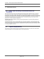
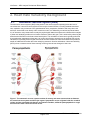
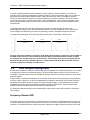
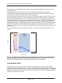
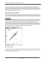
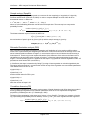
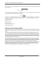
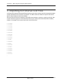
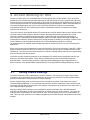
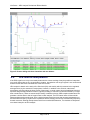
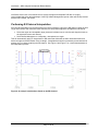
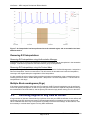
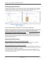
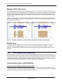
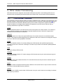
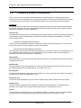
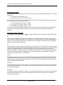
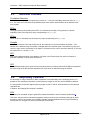
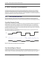
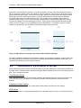
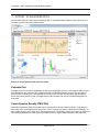
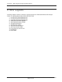
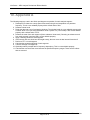
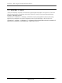
VivoSense™
User Manual – Heart Rate Variability (HRV)
Professional Edition
VivoSense™ HRV Professional Edition Version 2.0
Vivonoetics - San Diego Office
3231 Huerfano Court, San Diego, CA, 92117-3630
Tel. (858) 876-8486, Fax. (248) 692-0980
Email: [email protected];
Web: www.vivonoetics.com
VivoSense – HRV Analysis Professional Edition Module
Cautions and disclaimer
TM
VivoSense software is not a medical diagnostic tool. It is for research and investigational purposes only and
is not intended to be, or to replace, medical advice or review by a physician.
Copyright Notice
Copyright © 2012 Vivonoetics. All rights reserved.
User Documentation
HRV Standard Edition Module
Page 2 of 33
VivoSense – HRV Analysis Professional Edition Module
Table of Contents
1.
Introduction ............................................................................................................. 4
1.1.
Heart Rate Variability Professional Edition for VivoSense.............................................................. 4
1.2.
System Requirements ..................................................................................................................... 4
2.
Heart Rate Variability Background .......................................................................... 5
2.1.
Autonomic Nervous System (ANS) ................................................................................................. 5
2.2.
HRV Analysis Background .............................................................................................................. 6
3.
Importing R-R Interval Text Files .......................................................................... 11
4.
Artifact Marking for HRV ....................................................................................... 12
4.1.
Editing R-wave markings .............................................................................................................. 12
4.2.
R-R Interval Interpolation .............................................................................................................. 14
4.3.
Excluding Regions of Ecg Data as Artifact ................................................................................... 16
4.4.
Automated Artifact Marking ........................................................................................................... 18
4.5.
Artifact Statistics............................................................................................................................ 21
4.6.
Artifact Editing Layouts ................................................................................................................. 21
5.
HRV Data Processing ........................................................................................... 23
5.1.
Time Domain Channels ................................................................................................................ 23
5.2.
Frequency Domain Computation .................................................................................................. 24
5.3.
Nonlinear Channels....................................................................................................................... 26
5.4.
Respiratory Channels.................................................................................................................... 26
6.
HRV Channel Visualization................................................................................... 27
6.1.
HRV Window Selection ................................................................................................................. 27
6.2.
Calculations in the Presence of Artifact ........................................................................................ 28
7.
Other Visualizations .............................................................................................. 29
8.
HRV Exports ......................................................................................................... 30
9.
HRV Layouts ........................................................................................................ 31
10.
Appendix A ........................................................................................................... 32
11.
Works Cited .......................................................................................................... 33
User Documentation
HRV Standard Edition Module
Page 3 of 33
VivoSense – HRV Analysis Professional Edition Module
1. Introduction
1.1.
Heart Rate Variability Professional Edition for
VivoSense
This manual describes the heart rate variability (HRV) professional edition analysis module for VivoSense.
This module may be used to analyze and visualize several standard HRV indices. The manual includes a
background to the analysis of HRV, a description of the artifact editing capabilities included in the module and
a description of the various indices and methods of calculation and visualization. The module is delivered with
several layouts that facilitate the use of the HRV analysis. The module also allows for the export of HRV
parameters in a variety of possible configurations.
Familiarity with the core VivoSense module is an assumed prerequisite for use with the HRV professional
edition analysis module.
VivoSense HRV allows a user to visualize HRV indices of autonomic regulation, synchronized together with
relevant data channels from other sensors to provide a contextual significance to any research study. Further
automated and graphical artifact management capabilities allow for precise and accurate calculations of HRV
in a variety of application domains.
1.2.
System Requirements
This module is an add-on analysis module to VivoSense and requires the core module with a sensor import
module that supports an electrocardiogram (ECG) or R-R series waveform.
User Documentation
HRV Standard Edition Module
Page 4 of 33
VivoSense – HRV Analysis Professional Edition Module
2. Heart Rate Variability Background
2.1.
Autonomic Nervous System (ANS)
The autonomic nervous system (ANS) is the portion of the nervous system operating below the level of
consciousness. It acts as a control system for the body's visceral functions, including instantaneous heart
rate, respiration rate, movement of the gastrointestinal tract, perspiration, salivation and many other vital
activities. As the ANS is not directly under conscious control, it is affected by mental and emotional states.
It is of interest to many researchers to study the psychological states that influence the ANS and the analysis
of heart rate variability provides a non-invasive means to achieve this goal. This is achieved by observing the
affect that the ANS has on the beat to beat heart rhythm. The calculation of heart rate is typically performed
by averaging the instantaneous heart rate over a short time frame to smooth over the irregular beat to beat
variations. It is precisely these irregular moment-to-moment variations in heart rate however that provides a
wealth of additional information about the underlying autonomic function and balance. Heart rate variability
(HRV) is thus a measurement of these naturally occurring, beat-to-beat changes in heart rate.
Figure 1. The autonomic nervous system consists of sensory and motor neurons that run between
the central nervous system and the major organs. Sympathetic nerves originate inside the vertebral
column and are associated with thoracic and lumbar vertebrae, whilst the parasympathetic or vagal
division arises from cranial and sacral nerves.
User Documentation
HRV Standard Edition Module
Page 5 of 33
VivoSense – HRV Analysis Professional Edition Module
A number of health problems may be attributed in part to improper function or balance in the ANS. An
example of this is excessive sympathetic stimulation resulting in arterial constriction which can contribute to
hypertension and heart attacks. Measurements of HRV have thus been used to investigate autonomic
function in various affective disorders, and aberrant patterns of autonomic regulation. These have shown
promise in hypertension, congestive heart failure, heart transplantation, chronic mitral regurgitation, mitral
valve prolapse, sudden death or cardiac arrest, ventricular arrhythmias, supraventricular arrhythmias and
panic disorder.
In a healthy individual, the heart rate estimated at any given time represents the net effect of the
parasympathetic (vagus) nerves, which accelerates heart rate, and the sympathetic nerves, which slow it.
These changes are influenced by environment, pathology, emotions, thoughts and physical exercise.
A sample electrocardiogram (ECG) and describes how the HRV is determined is shown below.
46 BPM
49 BPM
54 BPM
1.3 seconds
1.2 seconds
1.1 seconds
Figure 2. Heart rate variability is a measure of the beat-to-beat changes in heart rate. The tall spikes in
the ECG are the R-waves. These control the electrical timing of the heart and the number of spikes
per minute is the average heart rate over that minute. These R-waves are not evenly spaced and the
timing of one R-wave to the following R-wave is called the R to R (R-R) or RR series. HRV analysis
seeks to quantify the variability in the R-R series.
2.2.
HRV Analysis Background
As described, changes in mental or emotional state result in changes to the ANS results, which in turn results
in changes to the beat to beat heart rate rhythm. The goal of HRV analysis is thus to work in reverse and
investigate a subjects affective state via the ANS by making inferences from a beat to beat time series of the
heart rate pattern.
A large number of specialized techniques for the analysis of HRV have been proposed by many researchers
all over the world. However in an effort to standardize the multitude of techniques, the European Society of
1
Cardiology and the North American Society of Pacing Electrophysiology in 1996 published a set of HRV
standards that the HRV professional edition VivoSense analysis module follows. These techniques are
divided into time and frequency domain calculations, discussed below.
For additional advanced techniques and methodologies, please refer to the premium edition of VivoSense
HRV analysis.
Frequency Domain HRV
The power spectrum of a time series is a representation of the frequency content within that time series. It is
a means of describing the power contained in every frequency. Thus if a selected R-R series has significant
variability, it is expected that there would be a greater contribution at higher frequencies relative to the lower
User Documentation
HRV Standard Edition Module
Page 6 of 33
VivoSense – HRV Analysis Professional Edition Module
frequencies that are associated with lower variability. This concept is formalized in the frequency domain
description of HRV.
A mathematical transformation is used to convert R-R data into a power spectral density (PSD)
representation. This power spectral transformation reduces the R-R signal into its constituent frequency
components and quantifies the relative power of these components.
The resulting power spectrum is then divided into three main frequency ranges. (see Figure 3). The very low
frequency range (VLF) (0.0033 to 0.04 Hz), represents the longer term, slower changes in heart rate in a
similar way to the average heart rate, and is sometimes used as an index of sympathetic activity. Due to the
low frequency variations, this index is best used in longer term recordings. The power in the high frequency
range (HF) (0.15 to 0.4 Hz) represents more rapid fluctuations in heart rate and is primarily influenced by
parasympathetic activity. The low frequency band (LF) is located between the VLF and HF bands and reflects
a mixture of sympathetic and parasympathetic activity, although it is frequently used to index sympathetic
modulation. It is more complex and is influenced by feedback from blood pressure signals sent from the heart
back to the brain.
Thus by calculating the power in these frequency ranges, it is possible to obtain some indication of ANS
function.
VLF
0.1
Low
Frequency
(LF)
High
Frequency
(HF)
Power [s2]
0.08
0.06
0.04
0.02
0
0.05
0.1
0.15
0.2
0.25
0.3
Frequency [Hz]
0.35
0.4
0.45
0.5
Figure 3. This figure shows a sample periodogram (averaged power spectrum) of the R-R waveform.
The power in each band is determined from the area under the curve over the frequency range of
interest and reflects the activity in the different branches of the nervous system.
Time domain indices
Several other commonly used HRV indices are based on simple statistics of the beat to beat variability.
These statistics tend to quantify the mean or variance of the variability over defined time intervals and may be
related to the frequency of the variability and hence an indirect measure of autonomic balance. The standard
deviation is a measure of all the changes in a time series, both high and low, and is directly mathematically
related to the total power in the series.
User Documentation
HRV Standard Edition Module
Page 7 of 33
VivoSense – HRV Analysis Professional Edition Module
Other time domain statistics are used to try and describe either the high or low frequency content in the
signals. For example, the standard deviation of the 5 minute means (SDANN) captures very slow changes
and is related to very low frequency changes. The root mean square of the differences (RMSSD) will be large
when there are large fluctuations in the consecutive differences and thus it is related to the high frequency
power and hence parasympathetic modulation.
Nonlinear measures of HRV
Advances in the analysis of nonlinear dynamics can be directly applied to the analysis of physiological time
series. It is now generally accepted that nonlinear methods can be more suitable to investigate more complex
underlying dynamics of the variations of the RR intervals. The nonlinear measures offered in VivoSense are:
Poincaré plots
The Poincaré plot displays RR(n+1) as a function of RR(n). In VivoSense, a Poincaré plot (see Figure 4) is
included in the Power Spectrum and Poincare layout.The screen dimensions of the plot are chosen to yield a
square shape in order to applying equal scaling to both x and y axis. In this plot short scale variations are
characterized by points lying far away from the line of identity (a radial line forming a 45⁰ angle). The
standard deviation of the distance of a points from the line of identity is denoted by SD1 and quantifies the
short term (i.e beat to beat) variations of RR. In addition, slow variations of the RR intervals are visualized as
points lining up along the line of identity. The standard deviation of the spread of the points along the line of
identity is denoted by SD2 and quantifies the long term variation of the RR intervals.
Figure 4: Poincaré Plot
In addition, the plot contains detailed beat to beat information such as outliers or clustering that cannot be
extracted from the measurement of SD1 and SD2. An ellipsis is drawn around the mean value of RR to aid in
the identification of physiological patterns.
User Documentation
HRV Standard Edition Module
Page 8 of 33
VivoSense – HRV Analysis Professional Edition Module
Sample entropy (SampEn)
Sample entropy (SampEn) was proposed as a measure for the complexity or irregularity of a signal by
Richman and Moorman (Richman JS, 2000). In order to compute SampEn one first forms all the m
dimensional vectors defined as
(
) where i = 1, 2, …N-m +1
where m is the embedding dimension and N is the RR sample size. The next step is to compute the
probability function
(
( )
)
The distance between a pair of vectors is defined as
[
]
the total number of pairs is given by (N-m+1)(N-m) and the sample entropy is given by
(
)
(
( ))
(
( ))
Detrended fluctuation analysis (DFA)
DFA is a method in stochastic processes to determine self-similarities of a time series on different time
scales. DFA is performed by first integrating the difference of RR time series minus the average of RR. This
series is then divided into subsets of length n. In each window a linear curve is fitted to the subset using a
least square fit. Then the root mean squared fluctuation of the difference of the series to the fitted curve is
calculated over the entire RR series to obtain a function F of the time scale parameterized by the subset
length n. The self-similarity factor α is obtained as the slope of F(n) plotted on a double logarithmic scale. VS
presents two such factors DFA α₁ and DFA α₂.
In VivoSense, this slope is determined by fitting F(n) using a linear regression on a double logarithmic plot.
The upper and lower limits of n, as well as the number of step of the regression are user defined parameters.
Their default values for DFA α₁ are:
n(upper limit) = 4
n(lower limit) = 16
and the default values for DFA α₂ are:
n(upper limit) = 4
n(lower limit) = 16
while the number of steps is 32.
Correlation dimension(CD)
The Correlation Dimension is a frequently used measure of fractal dimension and efforts have been made in
deriving pathological signatures from nonlinear parameters such as CD. VS implements the algorithm
proposed by Grassberger et al in (P. Grassberger, 1983).
The basis of the computation is the same set of vectors from SampEn. The idea is to compute a function
C(r) representing the probability that two arbitrary vectors and are closer together than the argument r.
( )
(
)
User Documentation
HRV Standard Edition Module
Page 9 of 33
VivoSense – HRV Analysis Professional Edition Module
The fundamental difference to SampEn is the use of the Euclidian metric to measure the distance d’ between
a pair of vectors:
[
]
√∑(
)
Chaotic signals have been shown to follow a power law ( )
the exponent D. The correlation dimension is defined as
where the dimensionality is quantified by
( )
In practice, it is determined by fitting D using a linear regression on a double logarithmic plot. The upper and
lower limits of r, as well as the number of step of the regression are user defined parameters in VivoSense.
Their default values are:
r(upper limit) = 0.06,
r(lower limit) = 0.16
Number of steps = 64
Embedding dimension M = 10
The time delay is fixed to 1.
Respiratory Sinus Arrhythmia (RSA)
There exists a natural cycle of heart rate variation that occurs through the influence of breathing on the flow
of sympathetic and vagus impulses to the sinoatrial node. This is cycle is termed respiratory sinus arrhythmia
(RSA).
The rhythm of the heart is primarily under the control of the vagus nerve, which inhibits heart rate and the
force of contraction. When we inhale, the vagus nerve activity is impeded and heart rate begins to increase.
When we exhale this pattern is reversed, that is the heart rate accelerates during inspiration and decelerates
during expiration. This alternating pattern of acceleration and deceleration corresponds to high frequency
changes in the R-R series and thus many researchers use the high frequency power as an index of RSA and
hence parasympathetic activity or vagal tone.
A number of laboratory studies, however, document that within-individual changes in respiratory parameters
of rate and tidal volume can seriously confound the association of RSA and cardiac vagal tone. Decreased
tidal volume and increased respiration rate can profoundly attenuate RSA under conditions in which cardiac
vagal tone remains constant. Thus measuring HRV to index RSA without simultaneously measuring
respiration may result in erroneous interpretation depending on the individual subjects breathing parameters.
Adjustment for respiratory parameters has been shown to improve relations between RSA and vagally
mediated heart rate and physical activity. In other words, concurrent monitoring of respiration and physical
activity enhances the ability of HRV to accurately estimate autonomic control.
User Documentation
HRV Standard Edition Module
Page 10 of 33
VivoSense – HRV Analysis Professional Edition Module
3. Importing R-R Interval Text Files
VivoSense HRV Analysis Professional Edition Module may be used to analyze data from supported hardware
formats described the the VivoSense Core Manual. The HRV module also allows for import of R-R Interval
files for further analysis of heart rate variability.
RR Interval files are text files containing a single RR Interval marking in seconds on each line of the file. Nonnumeric lines will be ignored. The RR Interval text file may be used to perform basic Heart Rate Variablity
analysis. An example of the format of the text file can be seen below:
0.9765034
0.9791907
0.9760966
0.9297528
0.9236943
0.9250374
0.9047443
0.9189222
0.9819303
1.034611
0.9886078
0.994711
0.9835241
1.020909
0.9838852
0.9268002
0.902474
0.8720775
…
User Documentation
HRV Standard Edition Module
Page 11 of 33
VivoSense – HRV Analysis Professional Edition Module
4. Artifact Marking for HRV
R-wave to R-wave (R-R) time series data channels markings will often contain artifacts. There are several
possible sources of artifact that may arise depending on the specific sensor used to generate the R-R series.
The raw sensor time series that the R-R series is derived from is typically an electrocardiogram (ECG) but RR data may also be derived from pulsephotoplethysmograhic (PPG) waveforms. Artifact will contaminate the
raw measured signal which may in turn result in erroneous detection of R-waves or corresponding
instantaneous heart rate. If the underlying raw data is contaminated it will not be possible to accurately
measure each heart beat.
The most commonly encountered artifact in R-wave detection is motion artifact. Other forms of artifact include
electrode movement with respect to the skin interface (disrupting electrochemical equilibrium); muscle
contraction resulting in unwanted electromyographic contamination that may share the desired signal
frequency band; vocalizations; temperature changes; sensor-cross-talk; optical path length changes and
electromagnetic induction. Different sensors have varying degrees of sensitivity to each type of artifact. Some
forms of artifact may be eliminated through the use of advanced filtering techniques and design
considerations such as shielded cables. Despite this however, artifact may still occur when measuring R-R
data series.
Errors in the location of the instantaneous heart beat will result in errors in the calculation of the HRV. HRV is
highly sensitive to artifact and errors in as low as even 2% of the data will result in unwanted biases in HRV
calculations. To ensure accurate results therefore it is critical to manage artifact and R-R errors appropriately
prior to performing any HRV analyses..
VivoSense provides several mechanisms for the management of artifact and the appropriate selection will
depend on the nature of the artifact. These different mechanisms and their recommended usage are
described below. The HRV Analysis module includes Ecg Artifact Management layouts appropriate for
different sensors in the “Modules\HRV Analysis\Dual Ecg” and “Modules\HRV Analysis\Single Ecg” folders.
4.1.
Editing R-wave markings
VivoSense calculates R-wave markings from an ECG waveform. If the waveform is noisy or has unusual
morphology due to arrhythmias, these markings may be erroneously calculated. The HRV analysis module
provides a mechanism to edit the location of R-wave markings.
R-wave marking editing must be performed from the actual R-wave channel. This channel is located in
“Electrocardiogram\Markings”. It is recommended that an ECG waveform channel be used to visually locate
erroneous markings and to correctly place new markings. This channel may be present on the same chart or
on an adjacent chart as preferred.
Manually editing R-wave markings is recommended for portions of the data where the QRS detection
algorithm may have failed, and the correct markings are clearly visible via visual inspection. This may occur
in the presence of EMG artifact or other sources of noise. This will typically occur for very short sections of
data. This is the most accurate form of artifact management prior to HRV analysis and should be performed if
possible.
User Documentation
HRV Standard Edition Module
Page 12 of 33
VivoSense – HRV Analysis Professional Edition Module
Deleting R-wave Markings
To delete an R-wave marking, the cursor must be located on a chart that includes a plot of the R-wave
marking. It is recommended to use the appropriate Ecg Artifact Management layout, which will identify
deleted R-wave markings as only the red outline, without the solid point. Position the cursor as close to the Rwave marking as possible and right click the mouse. Select Artifact Mangement->Edit Rwave->Delete. This
will delete the R-wave marking closest to the cursor. VivoSense will search for an Rwave marking within a
range of 0.1 seconds around the cursor. By default, an R-wave must be marked within a range of 0.1
seconds centered on the cursor for the menu item to appear. This distance is editable in the Rwave channel’s
Search Duration property. In addition, an annotation will be added to the annotation bar designating the
deleted R-wave marking. The annotation will be centered on the Rwave with default duration of 0.01
seconds, and all R-wave markings within the range of this annotation will be deleted. The default duration
may be modified with the Rwave channel’s Annotation Duration property. To undo this operation, right click
the mouse as close as possible to the deleted R-wave marking and select Artifact Mangement->Edit Rwave>Undo Delete.
Inserting R-wave Markings
To insert an R-wave marking, the cursor must be located on a chart that includes a plot of the R-wave
marking. It is recommended to use the appropriate Ecg Artifact Management layout, which will identify
insterted R-wave markings without the red outline. Position the cursor as close to the location where the Rwave marking should be and right click the mouse. Select Artifact Management->Edit Rwave->Insert. An Rwave marking will be inserted at the nearest peak within 50ms of the time at the cursor. In addition, an
annotation will be added to the annotation bar designating the inserted R-wave marking. To undo this
operation, right click the mouse as close as possible to the deleted R-wave marking and select Artifact
Mangement->Edit Rwave->Undo Insert. R-wave insertion uses the same Search Duration and Annotation
Duration properties as R-wave insertion.
Un-doing R-wave editing
Editing an R-wave marking does not alter the original R-wave channel, but rather modifies it in the areas
denoted by annotations. To undo multiple edits select a range on the R-wave channel including the edits to
delete and select Artifact Management->Edit Rwave->Undo Insert Annotations, or Artifact Management->Edit
Rwave->Undo Delete Annotations. Alternatively you may use the Annotation Manager to navigate, sort,
select and delete the annotations directly which will return those areas to the original R-wave channel.
Moving and Sizing R-wave edits
Sometimes it is desirable to have even more control over where the R-wave edit is placed. This can be done
by moving or sizing the Insert or Delete annotation by dragging and releasing the annotation itself on the
annotation bar. The result of the change will visible as you move or size the annotation. Delete edits may
delete multiple markings. Insert edits will always insert a single marking at the maximum value within the
annotation range. Delete edits always override insert edits. Edits saved in VivoSense prior to version 2.0 will
not be sizable or movable, so you will have to remove them and make new ones if you need this behavior.
User Documentation
HRV Standard Edition Module
Page 13 of 33
VivoSense – HRV Analysis Professional Edition Module
Figure 5. R-wave editing with three insertions and one deletion.
4.2.
R-R Interval Interpolation
If the ECG signal is too noisy to accurately determine the correct markings it may be possible to interpolate
over small regions that are one or two beats in duration. Interpolation over longer regions is not recommened
however as this will cause unwanted bias in the HRV results.
HRV analysis is based on the study of the Sino Atrial (SA) node activity which is assumed to be regulated,
amongst others, by the autonomic neural system. However, in addition to the SA node, other latent
pacemakers exist throughout the heart. Some of these may, in certain cases, introduce additional electrical
impulses that generate premature R-waves, typically resulting in a shorter R-R interval followed by a longer
than normal interval. These are termed ectopic beats. In addition to these, QRS complex misdetections can
generate a similar effect to that of ectopic beats in HRV analysis. The R-R interval trace will thus exhibit
sharp transients at the ectopic beat. Even a single isolated ectopic beat can alter spectral estimates due to
the broad-band frequency content of the impulse-like artifact, thereby erroneously overestimating frequencydomain measures. Although Ectopic beats result from accurate QRS detection, it is desirable to interpolate
over these beats prior to HRV analysis.
User Documentation
HRV Standard Edition Module
Page 14 of 33
VivoSense – HRV Analysis Professional Edition Module
VivoSense offers a set of convenient tools to quickly manage and interpolate R-R data. It is highly
recommended that users take advantage of the Ecg Artifact Management layouts, which will identify marked
artifacts with a dotted, red outline.
Performing R-R Interval Interpolation
R-R interval interpolation may be performed on any chart containing a plot of the RR channel. Using the time
range and minimum and maximum values selected, the interpolation algorithm will adjust the RR interval.


Select the region and acceptable range (select the left hand corner, left-click and drag the mouse to
the right hand corner and release).
Select Artifact Management > Interpolate > Interpolate over region
This will automatically apply an interpolation to RR values that fall below the lower horizontal border and
above the upper horizontal border of the rectangle. Interpolated areas will be marked by an annotation that
appears only on charts containing the RR channel. See Figure 6 and Figure 7 for a visual demonstration of
the interpolation process.
An ectopic beat
Figure 6. An ectopic beat has been found on the RR channel.
User Documentation
HRV Standard Edition Module
Page 15 of 33
VivoSense – HRV Analysis Professional Edition Module
Figure 7. An interpolation has been performed over the selected region, and an annotation has been
added to mark it.
Removing R-R Interpolations
Removing R-R Interpolations using the Annotation Manager
Interpolations may be removed by deleting the annotation associated with the interpolation in the annotation
manager. Note that it is possible to select and delete a group of interpolations.
Removing R-R Interpolations using the Context Menu
It is possible to right click on an R-R interpolation annotation and select “Artifact Management > Interpolate >
Remove interpolation” from the context menu. This will remove the annotation and undo the interpolation,
reverting to the original state prior to application of the interpolation.
It is also possible to select a range of data containing at least one interpolation using a rectangle and upon
releasing the mouse select “Artifact Management > Interpolate > Remove interpolations”. This will undo all
interpolations in the range.
Multiple Electrocardiograms (Ecgs)
If the sensor system supports more than one Ecg channel, the R-R interval interpolation may be performed
on the final primary RR channel, as well as any of the source RR channels. Separate interpolation markings
are maintained for each RR channel, and the primary RR channel simply allows viewing of one or the other.
4.3.
Excluding Regions of Ecg Data as Artifact
If large sections of data are contaminated by significant noise with poor QRS identification, these artifacts will
significantly bias HRV analyses and must be managed appropriately. Interpolating over large regions will
cause unwanted bias and it may not be possible to visually correct R-wave markings. In this instance, it will
be necessary to exclude these regions from any HRV calculations.
User Documentation
HRV Standard Edition Module
Page 16 of 33
VivoSense – HRV Analysis Professional Edition Module
Performing Artifact Exclusion
To exclude a region as artifact, select a range with the mouse on any chart containing raw Ecg, filtered Ecg,
or RR data. Upon releasing the mouse a context menu will appear. Select “Artifact Management > Exclude >
Exclude as artifact” to add an annotation and exclude this region from all calculations.
Figure 8. A region of artifact is selected by the user (left) and then excluded (right).
Please note: It is generally faster to mark exclusions on the RR channel as marking on any of the Ecg
channels requires the R-wave picker algorithm to be re-run. Additionally, RR artifacts will not
automatically be updated if edits are performed on the Ecg channel. Thus any Ecg markings should
be performed prior to undertaking RR artifact management.
Once unwanted artifacts have been excluded, the HRV algorithms will take these regions into account
adjusting the calculations accordingly to produce meaningful indices. For example if a 10 minute range has 1
minute excluded, the calculations will be performed on the remaining good 9 minutes rather than eliminate
the entire range as invalid data.
Removing Artifact Exclusions
Removing Artifact Exclusions using the Annotation Manager
Exclusions may be removed by deleting the annotation associated with the exclusion in the annotation
manager. Please note that it is possible to select and delete a group of exclusions.
Removing Artifact Exclusions using the Context Menu
It is possible to right click on an artifact exclusion annotation and select “Artifact Management > Exclude >
Remove exclusion” from the context menu. This will remove the annotation and undo the exclusion, reverting
to the original state prior to application of the exclusion.
It is also possible to select a range of data containing at least one exclusion using a rectangle and upon
releasing the mouse select “Artifact Management > Exclude > Remove exclusions”. In this way it is possible
to undo all exclusions in the range.
User Documentation
HRV Standard Edition Module
Page 17 of 33
VivoSense – HRV Analysis Professional Edition Module
Merging Artifact Exclusions
When dealing with automatically marked artifacts (see section 3.4), it may be necessary to clean the data to
achieve the desired, fully annotated data set. For example where a few seconds of apparently clean RR data
sits between two large areas of artifact. We determine upon further inspection, that this short period is also
artifact, VivoSense provides a simple way to merge the period and the surrounding exclusions into a single
period of artifact.
Using the mouse, select a range that encompasses the two exclusions. In the context menu that appears,
select “Artifact Management > Exclude > Merge exclusions”. The two exclusions will be expanded to include
the middle area. See Figure 9.
Figure 9. Two adjacent exclusions (left) have been merged into a single exclusion (right).
Multiple Ecgs
If the sensor system supports more than one Ecg channel, artifact exclusions may applied on any Ecg
channel, the final primary RR channel, as well as any of the source RR channels. Separate exclusion
markings are maintained for each RR channel, and the primary RR channel simply allows viewing of one or
the other.
4.4.
Automated Artifact Marking
Artifact marking is a complicated and time-intensive process that for now requires human intervention to
achieve the best results. In many cases, however, a significant portion of the artifact marking process may be
automated to provide an initial “best guess” pass that can then be quickly cleaned by the user. The automatic
artifact marking algorithm in VivoSense is not meant to be 100% accurate, but instead is a time-saving tool
that can be tuned to quickly mark artifacts to the user’s desired level of sensitivity.
Performing Automatic Artifact Marking
Automatic Artifact Marking using the Session Menu
To perform automatic artifact marking across an entire file, click on the “Session” menu and then choose
“Artifact Management > Automatic > Automatic Artifact Marking”. A window will appear displaying the options
that control the automatic artifact marking process. See Figure 10.
User Documentation
HRV Standard Edition Module
Page 18 of 33
VivoSense – HRV Analysis Professional Edition Module
Figure 10. The Automatic Artifact Marking options dialog.
The automatic artifact marking algorithm in VivoSense may be tuned by a small set of intuitive parameters to
best fit the needs of a particular file. The options available are:





Max HR (bpm) – This sets the maximum allowable heart rate. Areas with heart rates found above this
threshold will be marked as artifact
Min HR (bpm) – This sets the minimum allowable heart rate. Areas with heart rates found below this
threshold will be marked as artifact
Ectopic Beat Detection – Ectopic beats can bias HRV results. This setting determines whether
ectopic beats will be specifically detected and eliminated from the data
Noise Filtering – Signal noise from a variety of sources can bias or make data unusable. This setting
controls the level of filtering to be used
Max Interpolation Length – Long interpolations can bias data. When creating automatic markings,
this setting controls the maximum length for an automatic interpolation. Artifacts longer than this
threshold will be excluded
After the desired options have been selected, press the OK button to begin the process. When completed, a
statistics dialog will appear, detailing the markings created and their sources. See Figure 11.
User Documentation
HRV Standard Edition Module
Page 19 of 33
VivoSense – HRV Analysis Professional Edition Module
Figure 11. Statistics calculated over entire session after performing automatic artifact marking.
Press OK to close this dialog and view the results of the algorithm application. Using the annotation manager,
it is possible to browse all of the annotations created, and through the annotation description, also inspect the
reason for a particular marking made by application of the algorithm.
Automatic Artifact Marking using the Context Menu
Automatic artifact making may also be applied over a region, rather than an entire file. To do this, use the
mouse to select a region on any chart with an RR channel. In the context menu that appears, select “Artifact
Management > Automatic > Automatic Artifact Marking”. This will bring up the options screen and then
marking will proceed as normal. Please note: Statistics shown at the end of the process will be
calculated only over the region selected.
Undoing Automatic Artifact Marking
Undoing Automatic Artifact Marking using the Session Menu
To undo automatic artifact marking for an entire file, click on the “Session” menu and then choose “Artifact
Management > Automatic > Undo Automatic Artifact Marking”. All automatic artifact markings will be
removed, however, all user generated interpolations and exclusions will be left in place.
Undoing Automatic Artifact Marking using the Context Menu
To undo a single automatic artifact marking, right click on the desired marking’s annotation, and then in the
context menu choose “Artifact Management > Automatic > Undo Automatic Artifact Marking”.
Likewise, a group of automatic artifact markings can be removed together by dragging a region and then
selecting the same option from the context menu.
User Documentation
HRV Standard Edition Module
Page 20 of 33
VivoSense – HRV Analysis Professional Edition Module
4.5.
Artifact Statistics
It is possible to report statistics on the number and type of artifact markings.
Global Statistics
To report statistics for artifacts for the entire session, click on the “Session” menu and then choose “Artifact
Management > Statistics > Calculate”.
Regional Statistics
To report statistics for artifacts for a selected range, drag a rectangle area with the mouse over the desired
time span on any RR channel. Upon releasing the mouse, select “Artifact Management > Statistics >
Calculate” from the context menu.
Total count and percentage of area covered will be reported in a dialog box for each of the following statistics
(see Figure 11):







4.6.
RR artifacts/Automatic RR artifacts
Exclusions/Automatic exclusions
Interpolations/Automatic interpolations
Artifacts due to ectopic beats
Artifacts due to noise
Artifacts due to abnormal heart rate
Artifacts marked by the user
Artifact Editing Layouts
Artifact editing layouts are included in the professional HRV module to help streamline the artifact
management process. VivoSense contains three basic layouts, one for each of the Ecg signals in dual Ecg
hardware systems, and one for single Ecg systems.
To begin using a layout, open a file with Ecg data and then select the desired Ecg Artifact Management
layout from the HRV Analysis folder in the Layout Manager. Two charts will be placed on the screen – the
first shows the desired Ecg plot and its associated R-wave markings. The second chart displays the RR
intervals, derived from the Ecg data. See Figure 12.
One special plot that shows the original state of the data has been added to each of the charts. As edits are
made to either the Ecg, R-wave, or RR data, the user will be able to visualize exactly what changes have
been made and how these affect the data. In the Ecg chart, the original R-wave markings made by the Rwave picker are shown as a black square with a surrounding red box. User inserted markings will just show
the empty red box. Likewise, the original RR intervals will always be visible on the RR channel as a dotted
red line, even after interpolations and exclusions have been added.
User Documentation
HRV Standard Edition Module
Page 21 of 33
VivoSense – HRV Analysis Professional Edition Module
Figure 12. Artifact Management Layout.
User Documentation
HRV Standard Edition Module
Page 22 of 33
VivoSense – HRV Analysis Professional Edition Module
5. HRV Data Processing
HRV indices fall into two categories: time domain and frequency domain. In the following section we will
summarize the corresponding channels and discuss the steps used in the derivation of these parameters.
5.1.
Time Domain Channels
The terminology for these channels follows conventions established in the 1996 Task Force publication of the
1
European Society of Cardiology and the North American Society of Pacing and Electrophysiology . Here the
R-R interval data is termed N-N or NN data referring to the normal to normal sinus rhythm interval. Time
domain calculations are straight forward statistical computations on the RR interval channels and the
following calculations are provided in VivoSense.
SDNN
This is a standard deviation of the NN intervals, which is the square root of their variance. The variance is
mathematically equivalent to the total power of spectral analysis and thus it reflects all components of
variability and is an estimate of overall HRV.
RMSSD
This is the square root of the mean squared differences of successive intervals over a defined analysis
window. This measure quantifies high-frequency variations in heart rate in short-term recordings and may be
used as an estimate of parasympathetic modulation.
SDSD
This is the standard deviation of successive differences of NN intervals and quantifies high-frequency
variations in heart rate in short-term recordings. This index may be used as an estimate of parasympathetic
modulation.
ANN
This is the average of NN intervals.
SDANN
This is the standard deviation of 5 minute averages of NN intervals and may be used to estimate long term
components of HRV.
SDNNi
This is the mean of the standard deviation of 5 minute NN intervals and may be used to estimate long term
components of HRV.
NN50
This is the number of adjacent NN intervals with a difference of less than 50ms. It may be used in short term
recordings to estimate high frequency variations.
pNN50
This is the ratio of NN50 to total number of NN intervals. It may be used in short term recordings to estimate
high frequency variations.
User Documentation
HRV Standard Edition Module
Page 23 of 33
VivoSense – HRV Analysis Professional Edition Module
5.2.
Frequency Domain Computation
There are two commonly accepted methods described in the HRV literature for estimating the spectral
content of a time series: parametric and non-parametric methods. The results for both methods are available
in VivoSense and can be selected as a user editable property in any of the frequency domain channels.
Properties
The spectral function is shared by all the frequency domain channels and can be accessed and modified by
any of them. A change to any of the parameters described below above will affect all the frequency domain
channels simultaneously. These parameters are:
Estimation Type
The supported estimation types are: Autoregressive (AR), Welch (Scaled, to minimize frequency dependency
of the absolute values of the total power), and Welch (Unscaled, for backward compatibility). The default
value is Welch_Scaled.
Parametric (Autoregressive) Estimation
In the AR model, the parameter estimation is obtained by solving a set linear equations. The model order is
given by the number of the linear equations used in the estimation.
Non-Parametric (Periodogram) Estimation
The computation used is based on the Welch Periodogram. For each HRV interval, a new periodogram must
be computed and the indices derived. For a detailed list of all the necessary steps for the derivation of a
Power Spectral Density (PSD) estimate see Appendix A.
Window Width
The Window Width is the size of the individual estimation windows. It is measured as the number of samples.
The default value is 512.
AR Model Order
The autoregressive model order quantifies the number of linear equations solved by the model. There is no
corresponding parameter in the PSD estimate. The default value is 16.
Resampling Rate
Any RR signal is detrended, interpolated and resampled to an evenly spaced time series prior to processing.
The default value for the resampling rate is 3 Hz.
Interpolation Type
The choices for the interpolation type are Linear and Spline (cubic), with the default value being Spline.
Window Overlap
The PSD estimate is obtained as the average over multiple successive windows. The overlap of these
windows is user editable and is expressed as a relative fraction. The default value is 0.75.
Detrend
The entire data set is detrended prior to any estimation calculation. In addition, the user can decide whether
to detrend every window individually by setting the Detrend parameter to true (default) or false.
User Documentation
HRV Standard Edition Module
Page 24 of 33
VivoSense – HRV Analysis Professional Edition Module
Calculation of Indices
Once a PSD estimate is available, the power in the various frequency bands may be computed. The relevant
integrals are:
1. Total power (area under total curve)
2. Area under curve for VLF, LF and HF ranges
All other frequency domain indices are derived from these metrics. The default frequency ranges are given in
the Task Force paper and are summarized here:
1. Very low frequency (VLF) range: 0 - 0.04Hz
2. Low frequency (LF) range: 0.04Hz - 0.15Hz
3. High frequency (HF) range: 0.15Hz - 0.4Hz
These frequency ranges may be modified by the user. Please note: unlike the PSD parameters described in
the previous section, these frequency limits can only be accessed as a property of the corresponding
channels.
Frequency Domain Channels
1
The following indices are then computed and available as channels in the professional edition HRV module:
HF
High frequency variability, specifically due to respiration is on average between 0.15-0.4Hz.This measure
thus reflects the respiratory modulation on the heart rate or the RSA and is used to estimate parasympathetic
response. If more accurate measures of the respiration rate are available, they should be used to adjust the
HF band to reflect respiratory frequency.
LF
The recommended frequency range for the low frequency contribution is 0.04-0.15Hz. The power in this band
measure reflects both sympathetic and parasympathetic activity. However, it is thought to be a more accurate
indication of sympathetic activity in long-term recordings. The actual respiration rate may influence this
measurement and if an estimate of the true rate is available, it should be used to adjust this measure. Biases
may occur during particularly low respiration rates. This measure should be interpreted with caution and
examined in the context of the HF metric as well.
LF/HF
This measure is a ratio of the LF to HF component and indexes the overall balance between the sympathetic
and parasympathetic systems. Higher values reflect stronger sympathetic innervations, whilst lower values
indicate stronger vagal or parasympathetic influence. Like HF and LF, this parameter may be biased during
lower than average respiration rates.
HF(norm)
This measure minimizes the effect of changes in the very low frequency power and is used to index changes
in parasympathetic modulation. This measure is normalized and thus may be more suitable for comparisons
across a range of subjects.
LF(norm)
This measure minimizes the effect of changes in the very low frequency power and is used to index changes
in sympathetic modulation. This measure is normalized and thus may be more suitable for comparisons
across a range of subjects.
User Documentation
HRV Standard Edition Module
Page 25 of 33
VivoSense – HRV Analysis Professional Edition Module
5.3.
Nonlinear Channels
Correlation Dimension
The correlation dimension is computed using a value
for the embedding dimension and
. The value of CD increases as the data becomes more chaotic and decreases as the data becomes
more regular.
DFA α₁
The high frequency self-similarity factor DFA α₁ is obtained as the slope of F(n) plotted on a double
logarithmic scale in the frequency range corresponding to
.
DFA α₂
Same as DFA α₁ calculated over the frequency range corresponding to
.
SampEn
SampEn is a function of the total sample size N, the subset size m and the tolerance parameter r. The
sample size is determined by the number of samples within the selected region. Note that N may vary from
region to region even if the duration of the region is constant as in the case of trend-like channels. In VS uses
the subset size m = 10 and r = 0.15.
SD1
SD1 is the standard variation of the distance of all point in the Poincaré plot from the line of identity. It
quantifies variations in consecutive RR intervals.
SD2
The standard deviation of the spread of the points along the line of identity is denoted by SD2 and quantifies
the entire range of the RR intervals regardless of the time scale on which this range is reached.
5.4.
Respiratory Channels
An advantage of using VivoSense for HRV computation is that depending on the underlying sensor, it is
possible to use respiratory information to seed frequency ranges as well as to derive additional channels.
It is thus possible to manually adjust frequency ranges for the LF and HF channels based on the observed
respiration rate.
In addition, the following RSA channel is available:
RSA
2,3
This channel is calculated using the peak-valley method described in various academic publications .
This metric may be used to index parasympathetic activity over short term recordings. Although the index
provides a value for each breath, a more stable estimate of parasympathetic activity may be obtained by
trending this over a longer time interval containing several breaths.
User Documentation
HRV Standard Edition Module
Page 26 of 33
VivoSense – HRV Analysis Professional Edition Module
6. HRV Channel Visualization
VivoSense provides frequency domain HRV measures as data channels so that they can be visualized in
concert with other data channels in time on the synchronized chart panel. Vivonoetics terms this concept
VisualHRV™. HRV indices are always calculated from the R-R interval channel over a given time range. A
single index is computed for the entire time range that is used for computation. In VivoSense this single index
is typically visualized over the entire range as a staircase plot.
6.1.
HRV Window Selection
Any HRV indices are derived from the Power Spectral Density calculated over a particular window. As a
result, the visualization of HRV indices in the time-domain can be classified by the way the windows are
selected. The two methods used here are: trend-like (Trends directory) and user selected (Regions directory).
Trend-like Channels (Trends)
Using this method, each HRV index is calculated over a series of evenly spaced windows of equal width. The
parameterization and visualization is analogous to trend computations (see Figure 13). The properties of
Trend-like HRV channels that may be adjusted by the user include window duration and overlap duration.
To change the properties of all HRV channels, one has to select all the channels in the folder and adjust the
properties of the group selection. There are only two HRV folders that contain relevant indices: Time Domain
and Frequency Domain and Respiratory.
This method of analysis is a convenient way to track HRV changes over time in a general manner in the
same way that trended data may be explored.
HRV
Channel
R-R Interval
Channel
HRV Analysis
Interval
HRV Analysis
Interval
HRV Analysis
Interval
HRV Analysis
Interval
HRV Analysis
Interval
HRV Analysis
Interval
HRV Analysis
Interval
Figure 13. HRV channel as regular interval trend channel
User Selected Regions Channels
In performing HRV analyses, the user may frequently wish to examine the HRV over one or more well
defined user selectable intervals. Typically, these regions are not regularly spaced and they may not span the
entire file duration. This situation may be managed using a collection of channels located in the ‘Regions’
User Documentation
HRV Standard Edition Module
Page 27 of 33
VivoSense – HRV Analysis Professional Edition Module
directories in the Data Explorer window. To use this functionality, add any of the desired channels from the
HRV/ ‘sub’/Regions directory (here ‘sub’ stands for Frequency Domain, Time Domain of Respiratory) to the
synchronized chart panel (SCP). Then select a time range using the left mouse button and choosing ‘Select
HRV Region’ from the resulting pop-up menu. VivoSense will annotate the selected region of data and
compute all HRV indices over that particular region. This procedure can be repeated multiple times. A
previously selected region can be removed by right clicking within the corresponding region and selecting
‘Remove HRV Region’ from the resulting pop-up menu. Those regions not selected will not show any data
(NaN’s) as seen in Figure 14. No overlapping regions are allowed here. To calculate a single set of HRV
indices over the entire file, use the Session->Select HRV Region main menu option.
HRV
Annotation
HRV
Annotation
HRV
Channel
R-R Interval
Channel
HRV Analysis
Interval
HRV Analysis
Interval
Figure 14. HRV channel as irregular event channel with annotation markings
The HRV annotations will appear in the annotation manager. If an annotation is deleted, VivoSense will undo
the corresponding HRV calculation and replace the selected area with blank data (NaN). Please note: the
regions are shared among all the ‘Regions’ channels.
6.2.
Calculations in the Presence of Artifact
Artifact management allows either correction of artifact or removal of data that is contaminated by artifacts. In
the latter case, VivoSense is able to generate meaningful HRV indices based on the non-excluded portions of
data. This is managed as follows:
Time Domain Indices
This is handled the same way as the underlying statistics are managed (See VivoSense Core Manual). This
means that the index is calculated only on the set of available data. Any NaNs are excluded from the
analysis.
Frequency Domain Indices
For the Welch method, in step 5, any window that contains NaNs is excluded from the average.
RSA Indices
These are calculated on a breath by breath basis and are handled in the same way as Time Domain Indices.
User Documentation
HRV Standard Edition Module
Page 28 of 33
VivoSense – HRV Analysis Professional Edition Module
7. Other Visualizations
Several other charts are useful when visualizing HRV. To view these charts, load the Power Spectrum and
Poincare layout from the HRV Analysis folder.
Figure 15. Power Spectrum and Poincare Layout
Poincaré Plot
Poincaré Plots are a nonlinear visualization of HRV, by plotting RR[n+1] on the y-axis against RR[n] on the xaxis. Statistically, this represents the correlation between consecutive intervals. A set of axes are defined
about the line of identity (y=x). The nonlinear HRV indices SD1 and SD2 are calculated, and an ellipse is
drawn using these indices as radii. The appearance of the Poincaré Plot may be modified through the Plot
Properties.
Power Spectral Density (PSD) Plot
Power Spectral Density Plots are another way to visualize HRV over the frequency domain, by plotting the
RR Power on the y-axis against frequency on the x-axis. The frequency bands, represented by Shading, are
color coded yellow for VLF, green for LF, and magenta for HF. The Shading ranges and colors, as well as the
PSD Settings (independent of the frequency domain channels) may be edited through the plot properties.
User Documentation
HRV Standard Edition Module
Page 29 of 33
VivoSense – HRV Analysis Professional Edition Module
8. HRV Exports
To assist with the export of HRV data, several pre-configured exports are available in the VivoSense HRV
module. Exporting data using the standard core export functionality will allow the generation of HRV exports
that are meaningful. For example selecting a known range and exporting data in that range will provide a
table of HRV indices and the corresponding exported values. The preconfigured HRV exports under “HRV
Analysis” are:
1. Regions: all channels based on user selected regions
2. RSA: all RSA channels
3. Trends: all trend-like channels
User Documentation
HRV Standard Edition Module
Page 30 of 33
VivoSense – HRV Analysis Professional Edition Module
9. HRV Layouts
VivoSense software contains a collection of Layouts specific to the Professional Edition HRV Analysis
module. The following layouts are provided with this module:
1.
2.
3.
4.
5.
6.
7.
8.
9.
10.
11.
12.
Dual Ecg: Ecg1 Artifact Management
Dual Ecg: Ecg2 Artifact Management
Single Ecg: Ecg Artifact Management
HRV Frequency Domain Regions
HRV Frequency Domain Trends
HRV Nonlinear Regions
HRV Nonlinear Trends
HRV Time Domain Regions
HRV Time Domain Trends
Power Spectrum and Poincare
RSA Regions
RSA Trends
User Documentation
HRV Standard Edition Module
Page 31 of 33
VivoSense – HRV Analysis Professional Edition Module
10. Appendix A
The following steps are used in the Welch periodogram computation for each analysis segment.
1. Resample R-R channel to evenly spaced data series using linear interpolation at a particular
frequency. This is a user editable property with a default value of 3Hz.
2. Subtract a linear trend
3. Divide the data into a set of overlapping windows. The window length is a user editable property with
a default value of 512 (for best performance chose a power of 2). The overlap is also a user editable
property with a default value of 75%.
4. Subtract the mean from each segment (Some subtract a linear trend). Choosing to subtract a trend
from each segment is optional and is a user editable property.
5. Apply a Hanning window to each segment.
6. If the interval does not divide into this length exactly, then we move the last interval forward to fit
7. Perform a FFT on each segment
8. Calculate the squared magnitude of each segment
9. Take the average of all segments
10. Optionally scale by sample rate for frequency dependency. This is a user editable property.
11. Calculate the area under the curve between the specified frequency ranges. These are the indices
that are returned.
User Documentation
HRV Standard Edition Module
Page 32 of 33
VivoSense – HRV Analysis Professional Edition Module
11. Works Cited
1. Heart rate variability: standards of measurement, physiological interpretation and clinical use. Task Force
of the European Society of Cardiology and the North American Society of Pacing and Electrophysiology.
Circulation. 1996; 93(5):1043-65.
2. Grossman, P., Karemaker, J., & Wieling, W. Prediction of tonic parasympathetic cardiac control using
respiratory sinus arrhythmia: the need for respiratory control. Psychophysiology , 1991; 28; 201–216.
3. Grossman, P., van Beek, J., & Wientjes, C. A comparison of three quantification methods for estimation of
respiratory sinus arrhythmia. Psychophysiology , 1990; 27(6); 702-714.
User Documentation
HRV Standard Edition Module
Page 33 of 33