Download ExpEYES Programmer`s Manual

.
ExpEYES Programmer's Manual
Ajith Kumar B.P
Inter-University Accelerator Centre
New Delhi 110 067
Version 1 (May, 2011)
http://expeyes.in
1
Contents
1 Introduction
4
2 Hardware Communication
6
1.1 Software . . . . . . . . . . . . . . . . . . . . . . . . . . . . . . . . . . . . . . . .
2.1 Digital Inputs (ID0 and ID1) . . . . . . . . . . . . . . . . . . . .
2.1.1 read_inputs . . . . . . . . . . . . . . . . . . . . . . . . . .
2.2 Digital Outputs (OD0 and OD1) . . . . . . . . . . . . . . . . . .
2.2.1 write_outputs . . . . . . . . . . . . . . . . . . . . . . . . .
2.3 Analog Outputs . . . . . . . . . . . . . . . . . . . . . . . . . . . .
2.3.1 set_upv . . . . . . . . . . . . . . . . . . . . . . . . . . . .
2.3.2 set_current . . . . . . . . . . . . . . . . . . . . . . . . . .
2.3.3 set_bpv . . . . . . . . . . . . . . . . . . . . . . . . . . . .
2.4 Analog Inputs . . . . . . . . . . . . . . . . . . . . . . . . . . . . .
2.4.1 get_voltage . . . . . . . . . . . . . . . . . . . . . . . . . .
2.4.2 capture . . . . . . . . . . . . . . . . . . . . . . . . . . . .
2.4.3 capture01 . . . . . . . . . . . . . . . . . . . . . . . . . . .
2.5 Capture modiers . . . . . . . . . . . . . . . . . . . . . . . . . . .
2.5.1 disable_actions, enable_wait_high, (low, falling or rising)
2.5.2 enable_set_high, enable_set_low . . . . . . . . . . . . .
2.5.3 enable_pulse_high, enable_pulse_low . . . . . . . . . . .
2.6 Waveform Generation . . . . . . . . . . . . . . . . . . . . . . . . .
2.6.1 set_sqr1 . . . . . . . . . . . . . . . . . . . . . . . . . . . .
2.6.2 set_sqr2 . . . . . . . . . . . . . . . . . . . . . . . . . . . .
2.6.3 set_pulse . . . . . . . . . . . . . . . . . . . . . . . . . . .
2.7 Frequency Counters . . . . . . . . . . . . . . . . . . . . . . . . . .
2.7.1 digin_frequency . . . . . . . . . . . . . . . . . . . . . . . .
2.7.2 ampin_frequency . . . . . . . . . . . . . . . . . . . . . . .
2.7.3 sensor_frequency . . . . . . . . . . . . . . . . . . . . . . .
2.8 Passive Time Interval Measurements . . . . . . . . . . . . . . . .
2.8.1 r2ftime, f2rtime, r2rtime, f2ftime . . . . . . . . . . . . . .
2.8.2 multi_r2rtime . . . . . . . . . . . . . . . . . . . . . . . . .
2.9 Active Time Interval Measurements . . . . . . . . . . . . . . . . .
2
.
.
.
.
.
.
.
.
.
.
.
.
.
.
.
.
.
.
.
.
.
.
.
.
.
.
.
.
.
.
.
.
.
.
.
.
.
.
.
.
.
.
.
.
.
.
.
.
.
.
.
.
.
.
.
.
.
.
.
.
.
.
.
.
.
.
.
.
.
.
.
.
.
.
.
.
.
.
.
.
.
.
.
.
.
.
.
.
.
.
.
.
.
.
.
.
.
.
.
.
.
.
.
.
.
.
.
.
.
.
.
.
.
.
.
.
.
.
.
.
.
.
.
.
.
.
.
.
.
.
.
.
.
.
.
.
.
.
.
.
.
.
.
.
.
.
.
.
.
.
.
.
.
.
.
.
.
.
.
.
.
.
.
.
.
.
.
.
.
.
.
.
.
.
.
.
.
.
.
.
.
.
.
.
.
.
.
.
.
.
.
.
.
.
.
.
.
.
.
.
.
.
.
.
.
.
.
.
.
.
.
.
.
.
.
.
.
.
.
.
.
.
.
.
5
6
6
7
7
7
7
7
8
8
8
8
9
9
10
10
10
11
11
11
12
12
12
12
13
13
13
13
14
2.9.0.1 set2rtime, set2ftime, clr2rtime, clr2ftime
2.9.0.2 pulse2rtime, pulse2ftime . . . . . . . . .
2.9.0.3 set_pulse_width . . . . . . . . . . . . .
2.9.0.4 set_pulsepol . . . . . . . . . . . . . . .
2.10 Disk Writing . . . . . . . . . . . . . . . . . . . . . . . . .
2.10.1 save_data . . . . . . . . . . . . . . . . . . . . . .
3 Data processing
3.0.2 t_sine . .
3.0.3 t_dsine . .
3.0.4 t_exp . . .
3.0.4.1 t
.
.
.
.
.
.
.
.
.
.
.
.
.
.
.
.
.
.
.
.
.
.
.
.
.
.
.
.
.
.
.
.
.
.
.
.
.
.
.
.
.
.
.
.
4 Experiments
.
.
.
.
.
.
.
.
.
.
.
.
.
.
.
.
.
.
.
.
.
.
.
.
.
.
.
.
.
.
.
.
.
.
.
.
.
.
.
.
.
.
.
.
.
.
.
.
.
.
.
.
.
.
.
.
.
.
.
.
.
.
.
.
.
.
.
.
.
.
.
.
.
.
.
.
.
.
.
.
.
.
.
.
.
.
.
.
.
.
.
.
.
.
.
.
.
.
.
.
.
.
.
.
.
.
.
.
.
.
.
.
.
.
.
.
.
.
.
.
.
.
.
.
.
.
.
.
.
.
.
.
.
.
.
.
.
.
.
.
.
.
.
.
.
.
.
.
.
.
.
.
.
.
.
.
.
.
.
.
.
.
.
.
.
.
.
.
.
.
14
14
14
15
15
15
16
16
16
17
17
18
4.1 IV curve of a resistor . . . . . . . . . . . . . . . . . . . . . . . . . . . . . . . . . 18
4.2 Transient response of RC circuits . . . . . . . . . . . . . . . . . . . . . . . . . . 19
3
Chapter 1
Introduction
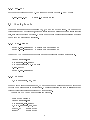
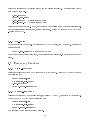
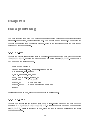
The design of expEYES is shown schematically in the block diagram below. Python functions
are available for accessing every feature of the expEYES hardware, like measuring a voltage
or frequency, setting a voltage or frequency, measuring time intervals etc. Data analysis and
graphics functions are given in two separate modules. Application programs are developed
using these modules.
The top panel showing the 32 Input/Output connectors.
4
1.1 Software
There are mainly three modules under the expeyes package:
• eyes.py : hardware communication
• eyeplot.py : Graphics using using Tkinter module
• eyemath.py : data analysis using modules numpy and scipy
They can be installed by using the .tgz les or the .deb packages provided on http://expeyes.in.
5
Chapter 2
Hardware Communication
The module expeyes.py contains all the functions required for communicating to the hardware
in addition to some utility functions. The functions are inside a class and the open() function
returns an object of this class if expEYES hardware is detected. After that the function calls
to access expEYES are done using this object, as shown in the example below.
import expeyes.eyes
# import the eyes library
p = expeyes.eyes.open() # returns an object if hardware is found
print p.get_voltage(0) # print the voltage at input A0
The hardware communication functions can be broadly grouped into analog inputs, analog
outputs, digital inputs, digital outputs, time interval measurements, waveform generation etc.
For making plots using the data from expEYES, we will use the matplotlib package1 .
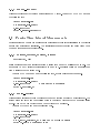
2.1 Digital Inputs (ID0 and ID1)
You can connect them externally to ground or 5 volts , to make the voltage level HIGH or
LOW. The software can read the voltage level present the inputs. A voltage less than 1 volt is
taken as a LOW or 0. Anything greater than 2 volts is treated as a HIGH or 1.
One of the powerful feature of digital inputs is the ability to measure the time between level
transitions with microsecond resolution.
2.1.1 read_inputs
Returns an integer whose 2 LSBs represents the voltage level present at the Digital Inputs ID0
& ID1.
print p.read_inputs() & 3
# print only the 2 LSBs
will print the number 3 ( 11bin ) if nothing is connected to the sockets, they are all internally
pulled up to 5 volts. With only ID0 grounded, the result will be 2, (10bin ).
1 You
can learn more about this package from http://matplotlib.sourceforge.net . The python book at
http://expeyes.in/sites/default/les/mapy.pdf gives an introduction to matplotlib.
6
2.2 Digital Outputs (OD0 and OD1)
You can set the voltage level on them to LOW or HIGH volts using software. The rst Digital
Output, OD0 is transistor buered and capable of driving up to 100 mA current but OD1 can
drive only 5 mA. If you connect LEDs to them, use a 1KΩ series resistor for current limiting.
2.2.1 write_outputs
The function takes an integer as argument whose 2 LSBs are used for setting the voltage level
on the four Digital Output sockets.
p.write_outputs(1)
p.write_outputs(2)
p.write_outputs(3)
# Sets OD0 HIGH
# Sets OD1 HIGH
# sets both HIGH
Measure the outputs with a voltmeter or by connecting an LED from the terminal to ground
with a 1kΩ resistor in series.
2.3 Analog Outputs
ExpEYES has two Programmable Voltage Sources, the Unipolar Programmable Voltage (UPV)
and the Bipolar Programmable Voltage (BPV). The voltage level on UPV can be set from 0
to 5V. The resolution is 12 bits, means the minimum step is around 1.25 mV. The voltage at
BPV can be set from -5 volts to +5 volts.
UPV is the direct output of a DAC. BPV is made from a unipolar signal using summing
circuits that may give some oset. If the requirement is only from 0 to 5 volts, use UPV.
2.3.1 set_upv
Set the output voltage of the UPV. The value of V should be from 0 to 5 volts
p.set_upv(2.5)
# Sets 2.5 volts on UPV
2.3.2 set_current
Set the output current at CS, between 0.05 mA to 1 mA. This function returns the voltage
at the current source output, that will be decided by the value of the external load resistor
connected. For example, setting 1 mA and connecting a 1kΩ resistor from CS to Ground, the
voltage read will be 1 volt (0.001A × 1000Ω) . The load and the current should be chosen such
that the product is less than 2 volts.
print p.set_current(1.0)
# prints the IR drop across the load.
Note: You can use either UPV ot CS at a time, since they share the same DAC output.
7
2.3.3 set_bpv
Set the output voltage of the BPV. The value of V should between -5 and +5 volts
p.set_bpv(-2.5)
# Sets -2.5 volts on BPV
2.4 Analog Inputs
There are four analog input channels: A0,A1,A2 and the SENsor input. We can read the
voltage level at any of this inputs, either as single reads or multiple reads in a single function
call, normally to capture a waveform. The time gap between consecutive reads inside a capture
can be set with microsecond resolution.
2.4.1 get_voltage
print p.get_voltage(0) # prints the voltage at A0
print p.get_voltage(2) # prints the voltage at A2
Connect BPV to A0 using a piece of wire and run the following program several times.
import expeyes.eyes
p = expeyes.eyes.open()
v = input('Enter V (-5 to 5)')
p.set_bpv(v)
print p.get_voltage(0)
2.4.2 capture
t,v = capture(ch, NP, tg)
where ch is the input channel number, NP is the number of measurements and tg is the time
between two measurements in microseconds. Two lists containing the time (milliseconds) and
voltage (volts) coordinates are returned by this function.
Connect SINE to A0 and run the following program.
from pylab import *
import expeyes.eyes
p = expeyes.eyes.open()
t,v = p.capture(0,300,100)
plot(t,v)
# from pylab
show()
# from pylab
8
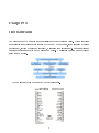
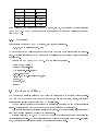
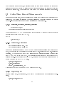
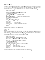
Terminal Channel # Range(V)
A0
A1
A2
SEN
CS
0
1
2
4
6
-5
-5
0
0
0
to
to
to
to
to
+5
+5
5
5
5
If the voltage to be measured is in the 0 to 5V range, use A2, that will give a better resolution
than A0 or A1. The SEN input is capable of measuring the value of a resistance connected
from it to GND.
2.4.3 capture01
This function captures A0 and A1 together, with timing correlation.
t,v,tt,vv = capture01(NP, tg)
NP is the number of measurements and tg is the time between two measurements in microsec-
onds. Four lists containing the two pairs of time (milliseconds) and voltage (volts) coordinates
are returned.
Connect SINE to A0 and SQR1 to A1. Run the following program.
from pylab import *
import expeyes.eyes
p = expeyes.eyes.open()
p.set_sqr1(100)
t,v,tt,vv = p.capture01(300,100)
plot(t,v)
plot(tt,vv)
show()
2.5 Capture modiers
The behavior of capture calls can be modied in several ways to enhance their exibility.
They can be made to start only when the input is between some specied limits, this feature
is essential for getting a stable trace for CRO applications.
You can also synchronize the beginning of digitization process with some external logical
signal. Digitization is made to wait for specied level changes on a digital input.
This feature is useful for digitizing transient waveforms. The synchronizing signal is derived
from the waveform itself and applied to a digital input.
It is also possible to SET, CLEAR or PULSE one of the digital outputs just before starting
the digitization process. The control functions only changes the settings at the micro-controller
end, the actions are visible only during the subsequent capture calls.
9
2.5.1 disable_actions, enable_wait_high, (low, falling or rising)
Calling this function makes all the subsequent capture and capture01 calls to wait for the
specied digital input socket to go HIGH / LOW before starting digitization. If that does not
happen, a timeout error will happen. Connect SQR1 to both A0 and ID0 and run the following
program.
from pylab import *
import expeyes.eyes
p = expeyes.eyes.open()
p.set_sqr1(100)
p.enable_wait_rising(0)
t,v = p.capture(0,200,100)
plot(t,v)
p.disable_actions()
t,v = p.capture(0,200,100)
plot(t,v)
show()
# wait for a LOW on ID0
# start at a rising edge
# removes all modifiers
# can start from anywhere
2.5.2 enable_set_high, enable_set_low
In some applications, it would be necessary to make a digital output socket go high/low before
digitization starts. This function, when called with a digital output socket number as argument,
makes the subsequent capture function set/clear OD0 or OD1 before it begins the capture
process. Action can be dened on only one digital output at a time.
Capturing the voltage across a capacitor while charging / discharging is a typical application
of this feature. Connect a 1uF capacitor between A0 and GND. Connect a 1KΩ resistor from
OD1 to A0 and run the following code.
from pylab import *
import expeyes.eyes
p = expeyes.eyes.open()
p.write_outputs(2)
# Take OD1 HIGH
p.enable_set_low(1)
# OD1 go LOW before capture
t,v = p.capture(0,200,20)
plot(t,v)
show()
The enable_set_low(2) makes OD1 to be taken HIGH just before digitizing the voltage on A0.
2.5.3 enable_pulse_high, enable_pulse_low
In some applications, it would be useful to send a PULSE on a digital output before digitization
starts. The enable_pulse_high() makes the specied output HIGH for some duration and then
10
makes it LOW. The duration is set by the set_pulsewidth() function. The calling program
should make sure that the socket is set to LOW before calling capture, else a HIGH to LOW
transition will result instead of a pulse. The enable_pulse_low() takes the output LOW and
then HIGH after some duration.
This function can be used to capture a waveform that is triggered by an input signal. For
example, connect the digital output OD1 to the input of a IC555 mono-shot circuit and connect
the 555 output to A0. Set the mono-shot delay to around a millisecond and run the following
code.
from pylab import *
import expeyes.eyes
p.write_outputs(2)
# OD1 to HIGH
p.set_pulse_width(1)
p.enable_pulse_low(1)
# LOW TRUE pulse
t,v = p.capture(0,300, 10)
plot(t,v)
show()
2.6 Waveform Generation
ExpEYES can generate square waves on SQR1 and SQR2. Variable duty cycle pulse of 488 Hz
can be generated on the PULSE output. The output SQR2 require an external variable resistor
for its operation.
2.6.1 set_sqr1
Generates a square waveform, having 50% duty cycle, on SQR1. The frequency can vary from
15Hz to 4MHz, but all intermediate values are not possible. The function returns the actual
frequency set.
import expeyes.eyes
p = expeyes.eyes.open()
print p.set_sqr1(1000)
print p.set_sqr1(1005)
The rst line will print '1000.0' but the second line will print '1008.06', that is the possible
frequency just above the requested one.
2.6.2 set_sqr2
Generates a square waveform on SQR2. The frequency can vary from .7Hz to 90 kHz in four
ranges. Setting the desired frequency will automatically select that range. Then you need to
11
adjust the external 22kΩ potentiometer to get the desired frequency. The actual value can be
read through software.
p.set_sqr2(10)
print p.get_sqr2()
p.set_sqr2(0)
# sets SQR2 to HIGH
p.set_sqr2(-1)
# sets SQR2 to LOW
will print anything between .7 to 25, depending on the position of the external potentiometer.
If no external resistor is connected, result will be zero. Setting 0 will make SQR2 HIGH and
-1 will make it LOW.
2.6.3 set_pulse
Sets the dutycycle of the 488.3 Hz pulse on the PULSE output, from 0 to 100%. Returns the
actual value set
print p.set_pulse(30) # duty cycle to 30%
Even though the requested value is 30, the actual value set will be 29.8% since it is done in 255
steps.
2.7 Frequency Counters
2.7.1 digin_frequency
Measure the frequency of a 0 to 5V square wave at ID0 or ID1. Connect SQR1 to ID0 and run
the following code
import expeyes.eyes
p = expeyes.eyes.open()
p.set_sqr1(500)
print p.digin_frequency(0)
2.7.2 ampin_frequency
Measure the frequency of a bipolar signal, amplitude > 100 mV, connected to Terminal 15.
Connect SINE to T15 and run the following code
import expeyes.eyes
p = expeyes.eyes.open()
print p.ampin_frequency()
The frequency of the sinewave will be printed.
12
2.7.3 sensor_frequency
Measure the frequency of voltage uctuations at SEN input. Connect SQR1 to SEN and run
the following code
import expeyes.eyes
p = expeyes.eyes.open()
p.set_sqr1(100)
print p.sensor_frequency()
2.8 Passive Time Interval Measurements
Digital Inputs can be used for measuring time intervals between level transitions on the digital
inputs with microsecond resolution. The transitions dening the start and nish could be on
the same terminal or on dierent ones.
2.8.1 r2ftime, f2rtime, r2rtime, f2ftime
r2ftime(in1, in2)
r2ftime returns delay in microseconds from a rising edge on in1 to a falling edge on in2. The
arguments ( 0 or 1) indicate digital inputs ID0 and ID1. Similarly f2rtime() measures time
from a falling edge to a riding edge.
Connect SQR1 to ID0 and run the following code, should print around 500 usecs.
import expeyes.eyes
p = expeyes.eyes.open()
p.set_sqr1(1000)
# half period = 500 usecs
print p.r2ftime(0,0)
2.8.2 multi_r2rtime
Measures time interval between two rising edges of a waveform applied to a digital input. The
second argument is the number of rising edges to be skipped between the two measured rising
edges. This way we can decide the number of cycles to be measured.
Connect SQ1to ID0 and run the following code.
import expeyes.eyes
p = expeyes.eyes.open()
p.set_sqr1(1000)
a = p.multi_r2rtime(0,9) # time for 10 cycles in usecs
print 10.0e6/a # frequency in Hz
13
For a periodic waveform input, the rst line returns the time for one cycle and the second one
returns the time for 10 cycles ( 9 rising edges in between skipped). This call can be used for
frequency measurement. The accuracy can be improved by measuring larges number of cycles.
2.9 Active Time Interval Measurements
During some experiments, we need to initiate some action and measure the time interval to the
result of it. The actions are initiated by setting, clearing or by sending pulses on the Digital
Outputs. The results will generate voltage transitions on Digital Inputs.
2.9.0.1 set2rtime, set2ftime, clr2rtime, clr2ftime
int set2rtime(out, in)
(remaining functions have similar prototypes)
These functions SET/CLEAR a digital output socket specied by out and wait for the digital
input specied by in to go HIGH /LOW.
USAGE
p.set2rtime(0, 1)
2.9.0.2 pulse2rtime, pulse2ftime
int pulse2rtime(int out, in)
int pulse2rtime(int out, in)
Sends out a single pulse on out (OD0 or OD1) and waits for a rising/falling edge on in (ID0 or
ID1). The duration and the polarity of the pulse is set by set_pulsewidth() and set_pulsepol()
functions. On powerup the width is 13 microseconds and polarity is positive ( voltage goes
from 0V to 5V and comes back to 0V). The initial level of out should be set according to the
polarity setting. If the polarity is LOW TRUE, the level must be set high beforehand and it
should be set low for HIGH TRUE pulse.
p.set_pulse_width(1)
p.set_pulsepol(1)
print p.pulse2rtime(0, 1)
measures the time from a pulse on OD0 to a rising edge on ID1.
2.9.0.3 set_pulse_width
Sets the pulse width, in microseconds, to be used by the pulse2ftime() and pulse2rtime() functions.
p.set_pulse_width(10)
14
2.9.0.4 set_pulsepol
Sets the pulse polarity to be used by the pulse2ftime() and pulse2rtime() functions. pol = 0
means a HIGH TRUE pulse and pol=1 means a LOW TRUE pulse.
p.set_pulsepol(1)
2.10 Disk Writing
2.10.1 save_data
Input data is of the form, [ [x1,y1], [x2,y2],....] where x and y are vectors, are save to a text
le.
Save the data returned by the capture functions into a text le. Default lename is `plot.dat',
that can be overriden by the second argument. Connect SINE to A0 and run the following code.
import expeyes.eyes
p = expeyes.eyes.open()
t,v = p.capture(0, 200, 100)
p.save([[t,v]], 'sine.dat')
open the le using the command
$xmgrace sine.dat
15
Chapter 3
Data processing
The data acquired from expEYES hardware is analyzed using various mathematical techniques
like least-square tting, Fourier transform etc. The module named eyemath.py does this with
the help of functions from the 'scipy' package. Most of the functions accepts the data format
returned by capture functions.
3.0.2 t_sine
Accepts two vectors [x] and [y] and tries to do a least-square tting of the data with the equation
A sin (2πf t + θ) + C . Returns the tted data and the parameter list[A, f, θ, C]. Connect SINE
to A0 and run the following code.
from pylab import *
import expeyes.eyes, expeyes.eyemath as em
p = expeyes.eyes.open()
t,v= p.capture(0,400,100)
vfit, par = em.fit_sine(t,v)
print par
# A, f, θ, C
plot(t,v)
# The raw data
plot(t,vfit)
# data calculated from par
show()
par[1] is frequency in kHz, since the time is given in milliseconds.
3.0.3 t_dsine
Accepts two vectors [x] and [y] and tries to do a least-square tting of the data with the
equation A = A0 sin (2πf t + θ) × exp(−dt) + C . Returns the tted data and the parameter
list[A, f, θ, C, d]. par[1] is frequency in kHz, since the time is given in milliseconds and 'd' is
the damping factor.
16
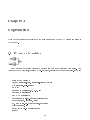
3.0.4 t_exp
Accepts two vectors [x] and [y] and tries to do a least-square tting of the data with the equation
A = A0 exp (kt) + C . Returns the tted data and the parameter list[A, k, C]. Connect a 1uF
capacitor from A0 to GND, 1kΩ resistor from OD1 to A0 and run the following code.
from pylab import *
import expeyes.eyes, expeyes.eyemath as em
p = expeyes.eyes.open()
p.write_outputs(2)
# Take OD1 HIGH
p.enable_set_low(1)
# OD1 go LOW before capture
t,v = p.capture(0,200,20)
plot(t,v)
vfit, par = em.fit_exp(t,v)
print par
plot(t,v)
# The raw data
plot(t,vfit)
# data calculated from par
show()
par[1] is the time constant RC in milliseconds.
3.0.4.1 t
Does a Fourier transform of a given data set. The sampling interval in milliseconds is the
second argument. Returns the frequency spectrum, ie. the relative strength of each frequency
component. Connect SINE to A0 and run the following code.
from pylab import *
import expeyes.eyes, expeyes.eyemath as em
ns = 1000 # number of points to be captured
tg = 100
# time between reads in usecs
p = expeyes.eyes.open()
t,v= capture(0, ns, tg)
x,y = em.fft(t, tg * 0.001) # tg in millisecs
plot(t,v)
# The raw data
plot(x,y)
# data calculated from par
show()
Modify this program to show the frequency spectrum of a square wave.
17
Chapter 4
Experiments
Most of the experiments described in the user manual can be done by writing few lines of
Python code.
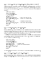
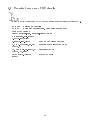
4.1 IV curve of a resistor
Make an array of current values and another one with same size lled with zeros. The
voltage at the CS terminal, returned by set_current(), is lled in to the second array. Both are
from pylab import *
import expeyes.eyes, expeyes.eyemath as em
p = expeyes.eyes.open()
NP = 20
current = linspace(.1, 2.0, NP)
voltage = zeros(NP)
for k in range(NP):
voltage[k] = p.set_current(current[k])
plot(current, voltage, 'x')
vf, par = em.fit_line(current,voltage)
plot(current, vf)
print 'R = %5.3f kOhm'%par[0]
show()
18
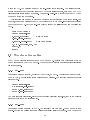
4.2 Transient response of RC circuits
We need to apply a voltage step at OD1 and immediately start capturing the voltage at A0.
NP = 200 # number of readings
tg = 10
# time gap between them, keep NP*tg around 3*RC
from pylab import *
import expeyes.eyes, expeyes.eyemath as em
p = expeyes.eyes.open()
p.write_outputs(2)
p.enable_set_low(1)
# OD1 go LOW before capture
t,v = p.capture(0,NP,tg)
# choose NP*tg according to RC
plot(t,v)
vf, par = em.fit_exp(t,v) # exponential fit
plot(t, vf,'r')
print abs(1./par[1])
# print RC value
show()
19