Download Innovative Experiments using Phoenix

.
Innovative Experiments
using
PHOENIX
Ajith Kumar B.P
Inter-University Accelerator Centre
New Delhi 110 067
&
Pramode C.E.
I.C.Software
Trissur, Kerala
Version 1 (2006)
1
Contents
1 Introduction
5
1.1
Objectives of PHOENIX . . . . . . . . . . . . . . . . . . . . .
5
1.2
Features for Developing Experiments . . . . . . . . . . . . . .
7
1.3
Microcontroller development system . . . . . . . . . . . . . . .
8
1.4
Stand-alone Systems . . . . . . . . . . . . . . . . . . . . . . .
9
2 Hardware and Software
10
2.1
The front panel . . . . . . . . . . . . . . . . . . . . . . . . . . 11
2.2
Things to be careful about when using Phoenix . . . . . . . . 14
2.3
Installing Software for PC interfacing . . . . . . . . . . . . . . 15
2.3.1
2.4
Software for programming ATmega16
Powering Up . . . . . . . . . . . . . . . . . . . . . . . . . . . . 16
3 Interacting with Phoenix-M
3.1
. . . . . . . . . 15
17
The Digital Outputs . . . . . . . . . . . . . . . . . . . . . . . 18
3.1.1
Blinking LED . . . . . . . . . . . . . . . . . . . . . . . 19
3.1.1.1
Exercise . . . . . . . . . . . . . . . . . . . . . 20
3.2
Digital Inputs . . . . . . . . . . . . . . . . . . . . . . . . . . . 20
3.3
Waveform Generation and Frequency Counting
3.4
Digital to Analog converter (DAC) . . . . . . . . . . . . . . . 22
3.5
Analog to Digital converter
. . . . . . . . 21
. . . . . . . . . . . . . . . . . . . 23
3.5.1
Introduction . . . . . . . . . . . . . . . . . . . . . . . . 23
3.5.2
Waveform Digitization . . . . . . . . . . . . . . . . . . 25
3.6
Time Measurement Functions . . . . . . . . . . . . . . . . . . 28
3.7
Non-programmable units . . . . . . . . . . . . . . . . . . . . . 29
2
3.8
3.9
3.7.1
Converting bipolar signals to unipolar . . . . . . . . . . 29
3.7.2
Inverting Op-Amps with externally controllable gain
3.7.3
Non-Inverting variable gain Amplier . . . . . . . . . . 31
3.7.4
The Constant Current Source Module . . . . . . . . . . 31
Plug-in Modules . . . . . . . . . . . . . . . . . . . . . . . . . . 32
3.8.1
16 character LCD display . . . . . . . . . . . . . . . . 32
3.8.2
High resolution AD/DA card
3.8.3
Radiation detection system
. . . . . . . . . . . . . . . 32
3.9.1
Light barrier . . . . . . . . . . . . . . . . . . . . . . . . 33
3.9.2
Rod Pendulum . . . . . . . . . . . . . . . . . . . . . . 33
3.9.3
Pendulum motion digitizer using DC motor . . . . . . 33
3.9.4
Temperature Sensors . . . . . . . . . . . . . . . . . . . 33
34
A sine wave for free - Power line pickup . . . . . . . . . . . . . 34
4.1.1
4.2
. . . . . . . . . . . . . . 32
Other Accessories . . . . . . . . . . . . . . . . . . . . . . . . . 32
4 Experiments
4.1
. 30
Mathematical analysis of the data . . . . . . . . . . . . 36
Capacitor charging and discharging . . . . . . . . . . . . . . . 38
4.2.1
Linear Charging of a Capacitor . . . . . . . . . . . . . 42
4.3
IV Characteristics of Diodes . . . . . . . . . . . . . . . . . . . 42
4.4
Mathematical operations using RC circuits . . . . . . . . . . . 44
4.5
Digitizing audio signals using a condenser microphone . . . . . 47
4.5.1
Exercise . . . . . . . . . . . . . . . . . . . . . . . . . . 48
4.6
Synchronizing Digitization with External 'Events' . . . . . . . 48
4.7
Temperature Measurements . . . . . . . . . . . . . . . . . . . 49
4.7.1
4.8
4.9
Temperature of cooling water using PT100 . . . . . . . 50
Measuring Velocity of sound . . . . . . . . . . . . . . . . . . . 53
4.8.1
Piezo transceiver . . . . . . . . . . . . . . . . . . . . . 53
4.8.2
Condenser microphone . . . . . . . . . . . . . . . . . . 55
Study of Pendulum . . . . . . . . . . . . . . . . . . . . . . . . 56
4.9.1
A Rod Pendulum - measuring acceleration due to gravity 57
4.9.2
Nature of oscillations of the pendulum . . . . . . . . . 57
4.9.3
Acceleration due to gravity by time of ight method . . 61
3
4.10 Study of Timer and Delay circuits using 555 IC . . . . . . . . 62
4.10.1 Timer using 555 . . . . . . . . . . . . . . . . . . . . . . 62
4.10.2 Mono-stable multi-vibrator
. . . . . . . . . . . . . . . 63
5 Micro-controller development system
5.1
5.2
Hardware Basics
65
. . . . . . . . . . . . . . . . . . . . . . . . . 67
5.1.1
Programming tools . . . . . . . . . . . . . . . . . . . . 68
5.1.2
Setting Clock Speed by Programming Fuses . . . . . . 68
5.1.3
Uploading the HEX le . . . . . . . . . . . . . . . . . . 70
Example Programs . . . . . . . . . . . . . . . . . . . . . . . . 71
5.2.1
Blinking Lights . . . . . . . . . . . . . . . . . . . . . . 71
5.2.2
Writing to the LCD Display . . . . . . . . . . . . . . . 72
5.2.3
Analog to Digital Converters . . . . . . . . . . . . . . . 74
5.2.4
Pulse width modulation using Timer/Counters . . . . . 75
6 Building Standalone Systems
76
6.1
Frequency Counter for 5V square wave signal
6.2
Room Temperature Monitor . . . . . . . . . . . . . . . . . . . 79
6.2.1
. . . . . . . . . 76
Exercise . . . . . . . . . . . . . . . . . . . . . . . . . . 81
7 Appendix A - Number systems
82
8 Appendix B - Introduction to Python Language
85
8.0.1.1
Exercises . . . . . . . . . . . . . . . . . . . . 91
9 Appendix C - Signal Processing with Python Numeric
96
9.1
Constructing a `sampled' sine wave . . . . . . . . . . . . . . . 97
9.2
Taking the FFT . . . . . . . . . . . . . . . . . . . . . . . . . . 98
10 Appendix D - Python API Library for Phoenix-M
4
101
Chapter 1
Introduction
Phoenix-M is an equipment that can be used for developing computer interfaced science experiments without getting into the details of electronics or
computer programming. For developing experiments this is a middle path
between the push − buttonsystems and the developf romscratch approach.
Emphasis is on leveraging the power of personal computers for experiment
control, data acquisition and processing. Phoenix-M can also function as a
micro-controller development system helping embedded system designs.
Phoenix-M is developed by Inter-University Accelerator Centre 1 . IUAC
is an autonomous research institute of University Grants Commission, India,
providing particle accelerator based research facilities to the Universities.
This document provides and overview of the equipment, its operation at
various levels of sophistication and several experiments that can be done
using it.
1.1 Objectives of PHOENIX
One may question the relevance of using a computer for experimental data
collection and advocate taking readings manually to improve the experimental skill of the students. The objective of Phoenix is to approach the process
1 Being
a product meant for the education sector, IUAC has granted permission for
commercial production of it without any royalty. For more details visitwww.iuac.res.in/
~elab/phoenix/vendors
5
of laboratory experiments from a dierent plane. Performing experiments
should be the fun part of learning science subjects but students at the college level do the traditional lab experiments by just following a given set of
inexible steps to take some measurements. Limitations of the apparatus
does not allow taking sucient data points involving fast changing parameters like position of a moving body or a uctuating temperature. This to a
major extent aects the accuracy of results, especially where the time measurements are concerned. Generally the students take three readings and
calculate the average value. The statistical error analysis techniques are
never done and are not possible owing to the lack of sucient data. One is
forced to make assumptions whose validity cannot be checked. The process
of experiments is more or less done like performing a ritual and the students
have no condence in the results they obtain.
A more important point is that the ability to perform experiments with
some condence in the results, opens up an entirely new way of learning
science. From the experimental data, students can construct a mathematical model and examine the fundamental laws governing various phenomena.
Research laboratories around the world performing physics experiments use
various types of sensors interfaced to computers for data acquisition. They
formulate hypotheses, design and perform experiments, analyze the data to
check whether they agree with the theory. Unfortunately the data acquisition hardware used by scientists is too expensive for college laboratories
where teaching is the main goal and not research. With the advent of inexpensive personal computers the only missing link is the data acquisition
hardware that is fast and sensitive enough to do physics experiments. If
such a data acquisition hardware is cheap enough then college level or even
school laboratories could aord to do experiments using computers and perform numerical analysis of the data. Physics with Home-made Equipment
and Innovative Experiments, PHOENIX is a step in that direction. Phoenix
provides microsecond level accuracy for timing measurements but the present
version gives only 0.1 % resolution for analog parameters, limited by the 10
bit ADC used.
The basic unit only provides an interface to the PC and the kind of ex6
periments you can do depends on the sensor elements available. The layered
software design does not demand much programming skills from the user. At
the same time we do not encourage the use of black boxes where you get the
results at the click of a mouse button. The approach is to get the data by
typing one or two lines of Python code.
Phoenix-M is the micro-controller based version of this interface which
also doubles as a training kit for electronics engineering and computer science students. Collecting data from the sensor elements and controlling the
dierent parameters of the experiment from the PC is one of the features
of Phoenix-M. This is achieved by loading the required software into the
micro-controller. At the same time the tools to change this resident code
also is being provided along with the system. This enables the students to
use it as a general purpose micro-controller development kit and designing
stand-alone projects.
1.2 Features for Developing Experiments
Phoenix-M oers the following features through the front panel sockets for
developing computerized science experiments.
1. Four channels of Analog Inputs
2. Programmable voltage source
3. Four Digital Inputs
4. Analog Comparator Input
5. Four Digital outputs (One with 100 mA drive capability)
6. Square Wave Generator (10 Hz to 4 MHz)
7. Frequency Counter ( 1 Hz to 1 MHz)
8. Constant Current Source (1 mA)
9. Two Variable Gain Inverting Ampliers
7
10. One Variable Gain Non-Inverting Amplier
11. Two Bipolar to Unipolar Converting Ampliers
12. 5V Regulated DC Output (from the external 9V DC input)
13. Serial Interface to PC
14. Easy to use Python language library
To develop science and electronics experiments suitable sensor elements are
wired to the front panel sockets and accessed from the PC using the Python
library. The program running on the micro-controller accepts the commands
from the PC, performs the tasks and sends the reply. Phoenix-M can run
on any computer with a Serial Port and a Python Interpreter with a library
to access the serial port. Free Software platforms like GNU/Linux is highly
recommended. Required software for both GNU/Linux and MS-Windows
are provided on the CD.
The system can also be used by booting from the Live CD without installing anything to the computer hard disk.
1.3 Microcontroller development system
This is another level of application of Phoenix-M and those who are only
interested in developing PC interfaced experiments may ignore it.
The
ATmeag16[1] microcontroller inside Phoenix-M can be programmed in C or
assembler. The program is compiled on the PC and the output hex format
le is uploaded to the micro-controller through a cable connected to the Parallel port of PC. The C compiler and development tools for this purpose are
provided on the CD for both GNU/Linux and MS-Windows operating systems. Most of the ATmega8 micro-controller Input/Output pins are available
through the front panel sockets. A 16 Character LCD Display is provided
along with C functions to access it. Details of using Phoenix-M as a microcontroller development system will be discussed in chapter 5.
8
1.4 Stand-alone Systems
The unit can be converted into standalone equipment like frequency counter,
function generator, temperature controller etc. by loading appropriate programs and using the sockets and the LCD display for Input/Output. Example
applications will be discussed in chapter 6.
9
Chapter 2
Hardware and Software
Phoenix-M kit comes with some accessories to try some simple experiments
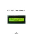
quickly. Verify that you get the following components with your Phoenix kit:
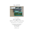
1. The Phoenix box (Figure 2.1)
2. 9V DC adapter
3. Serial port cable for communicating with the PC
4. Bootable CD containing Phoenix driver software and assorted tools
5. LED with resistor and three pins (one)
6. RC measurement cable with 4 pins (one)
7. 15 cm long wire with 2mm banana pins (three)
8. 25 cm long wire with 2mm banana pins (two)
9. Condenser microphone with biasing and signal cables (one)
10. 1 KΩ and 100 Ω resistors with pins, for variable gain amplier. (two+one)
11. 5V DC powered Piezo buzzer (without pin)
12. Metal lm Resistors 10 KΩ, 500Ω, 200Ω, 10Ω
The following accessories are available separately:
10
1. 16x1 LCD display
2. Parallel port cable for micro-controller programming
3. Diode Char Set (Setup to Study several PN junctions)
4. Light barrier (Time measurements by intercepting a beam of light)
5. Pendulum waveform digitizer using DC motor as transducer
6. Rod pendulum
7. PT100 temperature sensor
8. LM35 temperature sensor
9. 40KHz piezo transceiver pair ( for sound wave experiments )
10. 10 cm cable with pins (pack of 10)
11. 20 cm cable with pins (pack of 10)
2.1 The front panel
On the front panel you will nd several 2mm banana sockets with dierent
colors. Their functions are briey explained below.
1. 5V OUT - This is a regulated 5V power supply that can be used for
powering external circuits. It can deliver only upto 100mA current ,
which is derived from the 9V unregulated DC supply from the adapter.
2. Digital outputs - four RED sockets at the lower left corner . The
socket marked D0* is buered with a transistor; it can be used to drive
5V relay coils. The logic HIGH output on D0 will be about 4.57V
whereas on D1, D2, D3 it will be about 5.0V. D0 should not be used in
applications involving precise timing of less than a few milli seconds.
11
Figure 2.1: The Phoenix-M box
12
3. Digital inputs - four GREEN sockets at the lower left corner. It might
sometimes be necessary to connect analog outputs swinging between
-5V to +5V to the digital inputs. In this case, you MUST use a 1K
resistor in series between your analog output and the digital input pin.
4. ADC inputs - four GREEN sockets marked CH0 to CH3
5. PWG - Programmable Waveform Generator
6. DAC - 8 bit Digital to Analog Converter output
7. CMP - Analog Comparator negative input, the positive input is tied
to the internal 1.23 V reference.
8. CNTR - Digital frequency counter (only for 0 to 5V pulses)
9. 1 mA CCS - Constant Current Source, BLUE Socket, mainly for Resistance Temperature Detectors, RTD.
10. Two variable gain inverting ampliers, GREEN sockets marked IN and
BLUE sockets marked OUT with YELLOW sockets in between to insert
resistors. The ampliers are built using TL084 Op-Amps and have a
certain oset which has to be measured by grounding the input and
accounted for when making precise measurements.
11. One variable gain non-inverting amplier. This is located on the bottom right corner of the front panel. The gain can be programmed by
connecting appropriate resistors from the Yellow socket to ground.
12. Two oset ampliers to convert -5V to +5V signals to 0 to 5V signals.
This is required since our ADC can only take 0 to 5V input range.
For digitizing signals swinging between -5V to +5V we need to convert
them rst to 0 to 5V range. Input is GREEN and output is BLUE.
To reduce the chances of feeding signals to output sockets by mistake the
following Color Convention is used
• GREEN - Inputs, digital or analog
13
• RED - Digital Outputs and the 5V regulated DC output
• BLUE - Analog Outputs
• YELLOW - Gain selection resistors
• BLACK - Ground connections
2.2 Things to be careful about when using Phoenix
1. The digital output pins can drive only 5mA. Don't connect any load
less than 1K Ohm to them.
2. Digital output D0 is transistor buered and can provide 100 mA. Don't
use it for timing controls.
3. Digital and ADC inputs should not be negative or above 5V, ie. should
be from 0 to 5V.
4. Variable gain amplier outputs should be connected to Digital Inputs
only through a One KOhm series resistor.
5. Amplier inputs should be within -5 to +5V range.
6. Output pins should not be tied together.
7. Do not draw more than 100mA current from the 5V regulated supply.
Take necessary protections against back emf when connecting inductive
loads like motors or relay coils.
8. Forcibly Inserting Multi Meter probes with diameter more than 2 mm
to the front panel sockets will damage them.
9. And, don't pour coee into the sockets !
14
2.3 Installing Software for PC interfacing
There is no need to install any software if you plan to use Phoenix-M by
booting from the Live CD. Otherwise on a GNU/Linux distribution you need
to install the pyserial module and the phm.py module. To install pyserial
, unzip the le pyserial − 2.2.zip, located inside the directory P hoenix −
M/Linux on the CD, into a directory and run the following commands from
that directory.
#python setup.py build
#python setup.py install
To install the phoenix-M library just copy the le phm.py to directory named
site − packages inside the python directory.
1
On MSWindows install the les inside the directory M Swin on the CD,
by clicking on them, and copy phm.py to the directory named lib inside the
python directory (python24 inside the root directory of C: drive) .
2.3.1 Software for programming ATmega16
Again there is no need to install any software if you are working from the
live CD. Otherwise you need to install the AVR GCC compiler and other
development tools. On GNU/Linux systems that supports installing 'rpm'
les , goto the Linux/RPM directory on the CD and run the install script by
typing,
#sh install.sh
This will install all the necessary tools for software development on AVR
micro-controllers including ATmega16. On MS-Windows run the self extracting archive W inAV RGCC.exe to install the development suite. Example programs are available inside directory cprogs on the CD.
1 On
most systems this will be /usr/lib/python2.x, where x is the version number
15
2.4 Powering Up
Connect the the provided serial cable between the 9 pin D connector on the
Phoenix box and COM1 (rst serial port) of the PC2 . Connect the 9V DC
adapter to the socket on the Phoenix box and apply power. The power LED
near the 5V socket should light up. The easiest way to use Phoenix-M is
to boot the PC with the supplied GNU/Linux live CD; you will get a text
prompt along with instructions on how to proceed further.
Enter graphics mode by running the commands `xconf' followed by `startx'.
You can read various documents concerning Phoenix-M and other other educational tools by simply running the browser. Start a command shell and
you are ready to get into the fascinating world of Phoenix-M!3
2 If
COM1 is not available, you can use COM2, but you will have to make a very small
change during library initialization
3 If you using it under MS-Windows install Python Interpreter , Pywin32, Pyserial
and Phoenix library modules provided on the CD. Phoenix Library 'phm.py' should be
copied to the directory 'Python24\lib' .Start python from the command prompt by typing
'python24\python' at the 'C:\>' prompt.
16
Chapter 3
Interacting with Phoenix-M
This chapter is a tutorial introduction on accessing Phoenix-M from the PC
using the Python Library. The emphasis is on getting familiar with hardware
and software features rather than doing actual experiments. Phoenix-M library functions are explained in Appendix D and a brief introduction to the
Python programming language is given in Appendix B. It is assumed that
Python Interpreter and Phoenix-M library are installed and the equipment
is connected to the serial port of the PC.
Start the Python Interpreter from the command prompt. You should see
something like the following
Python 2.3.4 (#1, Oct 26 2004, 16:42:40)
[GCC 3.4.2 20041017 (Red Hat 3.4.2-6.fc3)] on linux2
Type "help", "copyright", "credits" or "license" for more information.
>>>
The rst step is to import the phoenix library and create and object of type
class 'phm'. This is done by the the following lines of code
> > > import phm
> > > p = phm.phm()
The variable 'p' is an object of class 'phm' and represents the Phoenix box
in software. These two lines must be present in the beginning of all Python
17
programs accessing Phoenix-M. Let us start by accessing the features of
Phoenix-M one by one.
Again we remind you NOT to connect any signals greater than 5 VOLTS
to Phoenix-M.
3.1 The Digital Outputs
You should see four sockets labeled D0 to D3 in a section marked `Digital Outputs'. It's possible to make these pins go high and low under program
control.
Invoke the Python interpreter and enter the following lines:
> > > p.write_outputs(0)
Connect an LED and a 1K Ohm resistor in series between digital output pin
D3 and ground1 (any one of the Black sockets) - make sure that the longer
leg (the anode) of the LED is connected to D3. You will see that the LED
is OFF. Now, type the following line:
> > > p.write_outputs(8)
You will see that the LED has lighted up! Want to put it o? Type:
> > > p.write_outputs(0)
again! What is happening here?
> > >p.write_outputs(8)
we are asking the Phoenix box to write the number 8 to the digital output
lines. Now, what does that really mean?
The number 15 can be expressed as 1000 in binary - let's call the rightmost
bit `bit0' or the least signicant bit and the leftmost bit `bit3' or the most
1A
single strand wire with a bit of insulation stripped o its end and bent into a thin
hook can be conveniently inserted into the Phoenix connectors. The LED and resistor can
be placed on a breadboard.
18
signicant bit. The value of these bits have a relation to the voltages on
digital output pins D0 to D3. If bit0 is 1, the voltage on D0 will be +5V and
if it is 0, the voltage would be 0V. Thus, when we write 8, bit3 is 1 and the
output on pin D3 will be high2 .
If you are new to binary arithmetic, make sure that you understand this
clearly3 .
Exercises
1. With a multimeter (or LED's), verify which all pins are high/low when
you execute p.write_outputs(10). Is D0 dierent ?
2. How would you call p.write_outputs() if you want D0 and D3 to be
high and all other pins low?
3.1.1 Blinking LED
It's time to make the LED blink! Type the following code at the Python
prompt:
> > > import time
> > > while 1:
p.write_outputs(1)
time.sleep(1)
p.write_outputs(0)
time.sleep(1)
...
>>>
The logic is easy to understand - writing a `1' results in digital output pin
D0 going high; we then delay execution for one second by calling the `sleep'
2 The
socket marked D0* is buered using a transistor and can be used for driving 5V
relay coils. This output works well only with some load connected to ground. The HIGH
level voltage of D0 is slightly less than 5V due to the transistor.
3 This is absolutely important - unless you understand this idea properly, you will not
be able to do anything with the Phoenix box
19
routine - the LED stays high during this period. We then make it go low by
writing a `0' and again sleeps for 1 second. The whole process gets repeated
innitely. Press Ctrl-C to come out of the loop.
3.1.1.1 Exercise
Connect an LED each (in series with a 1KOhm resistor) between digital
output pins D0, D1, D2, D3 and ground. Write a Python program to make
these LED's light up (and go o) sequentially.
3.2 Digital Inputs
The Phoenix box is equipped with four digital input pins labeled D0, D1, D2,
D3 (look at the section of the panel marked `DIGITAL INPUTS'). Execute
the following Python code segment and repeat it after connecting a wire from
D3 (GREEN socket) to Ground.
> > > p.read_inputs()
15
> > >p.read_inputs()
7
How do we interpret the results. If we express 15 and 7 in binary forms, we
get the bit patterns:
1111 and 0111
According to our convention, we call the rightmost bit `bit0' and the leftmost
bit, `bit3'. If `bit3' is 1, it means that the voltage on digital input pin D3 is
HIGH4 , ie +5V and if it is 0, it means that the voltage on D3 is LOW, ie,
0V. Similar is the case with all the other bits. All bits are internally pulled
up to 5V and we got the 15 , when D3 is grounded we got 7.
Another experiment. Connect digital output pins D3 to the digital input
pins D3. Execute the following code fragment:
4 We
will follow this HIGH means +5V and LOW means 0V convention throughout
this document.
20
>>>
>>>
7
>>>
>>>
15
p.write_outputs(0)
p.read_inputs()
p.write_outputs(8)
p.read_inputs()
It's easy to justify the results which we are getting!
The digital inputs are versatile - We will come to the time measurements
with microsecond accuracy using them.
3.3 Waveform Generation and Frequency Counting
Identify the socket marked `PWG' (Programmable Waveform Generator) on
the Phoenix box. Now execute the following command at the Python prompt:
> > > p.set_frequency(1000)
1000
>>>
This results in a 1000Hz (0 to 5V) square waveform being generated on
PWG5 . If you have a CRO, you can observe the waveform on it. An easier
way is to simply connect the PWG socket to a socket marked `CNTR' - the
Phoenix box has a built-in frequency counter which can measure frequencies
upto 1 MHz. Measuring frequency is simple - once the signal is connected to
the CNTR socket, execute the following Python function:
> > > p.measure_frequency()
1000
>>>
5 It
is possible to set frequencies from 15Hz to 4MHz - but it need not always set the
exact frequency which you have specied, only something close to it. The actual frequency
set is returned by the function.
21
In this case, we are getting 1000, which is the frequency of the waveform on
the PWG socket. If you have a 0 to 5V range Square wave you can measure
its frequency using this call. You can measure the frequency of an external
oscillator signal by connecting it to the CNTR input , provided it is a 0 to
5V signal. Measuring frequency using the Digital input sockets and Analog
Comparator Socket will be discussed later.
3.4 Digital to Analog converter (DAC)
An analog output voltage ranging from 0 to +5V can be programmed to the
socket marked PVS, Programmable Voltage Source. Execute the following
lines of code and measure the output with a multimeter after each step.
> > >p.set_dac(0)
> > >p.set_dac(128)
> > >p.set_dac(255)
The output can be varied from 0 to 5V in 256 steps. When using this function,
you need to calculate the number to be used for a given voltage. This can
be avoided by using
> > >p.set_voltage(2000)
The output should now measure near 2000 millivolts. Remember that you
can set the voltage in steps of nearly 20 mV only since 5000 mV range is
covered in 256 steps.
The DAC on the Phoenix box is made by ltering the Pulse Width Modulated signal from the Programmable Waveform Generator, PWG. Due to this
one can't use both PWG and DAC at the same time. If you call 'set_dac()'
while a waveform is being generated on the PWG, it's frequency will change.
Similarly, if you call `set_frequency()' after xing a specic voltage level on
the DAC, the voltage will change.
22
3.5 Analog to Digital converter
3.5.1 Introduction
Analog to Digital converters are a critical part of computerized measurement
and control systems. Let's say we wish to measure temperature - a sensor
like the LM35 converts temperature in degree Celsius to voltage in milli volts
at a rate of 10mV per degree Celsius. Thus, if room temperature is 27 degree
Celsius, the sensor output would be 270mV. An ADC helps us convert this
voltage into a numerical quantity. Let's see how.
Say the minimum voltage we would like to measure is 0V and maximum
is 5000mV (ie, 5V). Let's divide this 0 - 5000 range into 256 discrete steps,
each step of `size' 19.53 (ie, 5000.0/256). The zeroth step is from 0 to 19.53,
the rst step from 19.53 to 39.06 and so on ... If we have a device which
accepts as input a voltage in the range 0 to 5000mV and returns the number
of the step to which the input belongs to, our objective of converting the
analog input to digital is achieved! An 8 bit (8 bits give you 256 dierent
numbers from 0 to 255) ADC does exactly this. We call the number `8' the
`resolution' of the ADC.
We note that there is a certain amount of inaccuracy in the conversion
process - an 8 bit ADC will resolve all voltages in a certain `step' to one
particular step number - thus, you will not be able to dierentiate whether
your input was exactly 0mV, or 1mV or 2mV or 19.53mV - all these inputs
simply map to step zero.
A 10 bit ADC can do a better job - as 10 bits can hold numbers from 0
to 1023 (1024 combinations), a 0 to 5000mV range can be broken down into
steps of size 5mV each.
Analog inputs are one of the important features of Phoenix-M. There are
four channels of Analog inputs that can digitize a voltage between 0 to 5V.
Feeding a voltage outside these limits may damage the micro-controller. The
Analog to Digital Converter resolution can set by the user (default is 8 bit).
The speed of the ADC (the time it takes to convert an analog input to digital)
also can be set within certain limits. To explore the ADCs, connect the DAC
23
output to channel zero of the ADC and issue the following commands
> > >p.set_dac(200)
> > >p.select_adc(0)
> > > print p.read_adc()
(1148439372.3935859, 199)
The select_adc() function is used for selecting the channel to which we have
connected the input. The read_adc() call returned two values instead of one.
The rst is the system time stamp from the PC (we are not concerned with it
at present) and the second is the output of the ADC received from PhoenixM. The value is not 200 but 199, this is mainly due to the limitations of the
DAC. The above exercise can be done more conveniently by the following
functions.
> > > p.set_voltage(4000)
> > > m = p.zero_to_5000()
> > > print m
(1148440112.655, 4019.6078431372548)
> > > print m[1]
4019.6078431372548
The zero_to_5000() function converts the ADC output into milli volts, the
rst number in the output is again the time stamp from PC.
The maximum resolution of the ADC output is 10 bits but it can be
reduced to 8 bits for faster data transfer. The conversion time of the ADC
also can be set by the user by calling `p.set_adc_delay'. When set to 10 bit
resolution the conversion time should be set to larger than 200 microseconds.
If we wish to measure static (or slowly changing) parameters like temperature
accurately, we better use 10 bit resolution and a conversion delay of over 200
micro seconds. If the objective is to visualize (plot a graph of) a fast varying
signal, it is better to use 8 bit resolution and a conversion delay of 10 micro
seconds.
We will do one or two experiments to have a better idea of how things
work. First, connect digital output D3 to ADC channel 0 and execute:
24
> > > p.write_outputs(15)
> > > p.set_adc_size(2)
> > > p.set_adc_delay(200)
> > > p.select_adc(0)
> > > p.read_adc()
1023
> > >p.zero_to_5000()
(1148537333.2460589, 5000.0)
The ADC is now working in 10 bit mode (the function call 'p.set_adc_size(2)'
does this) - digital output pin is high (close to +5V), ADC range is 0 to
5000mV - so the ADC will output a value close to 1023 (maximum possible
10 bit number). The zero_to_5000() function converts the output of the
ADC into voltage from 0 to 5000 mV irrespective of the adc data size (8 ro
10 bits).
> > > p.set_adc_size(1)
> > > m = p.read_adc()
> > > print m[1]
255
The ADC is now working in 8 bit mode (maximum output is 255) - the range
is 0-5000mV and the input is close to 5V - so the output should be close to
255.
3.5.2 Waveform Digitization
In certain applications, you will be required to capture data from one (or
more) ADC channel(s) in bulk (say 200 samples) at precisely timed intervals.
There are functions available in the Phoenix library to do exactly this.
There are two important block read functions - `read_block' and `multi_read_block'.
We will examine `read_block' rst. Connect 5V to ADC channel 0 and execute the following code fragment:
> > > p.select_adc(0)
25
> > > p.set_adc_size(1)
> > > m = p.read_block(100, 50, 0)
> > >print m
We are basically asking the Phoenix box to take 100 readings from the ADC
,from the currently selected channel, with an inter-read delay of 50 microseconds. The last argument to read_block will be 1 only when we are analyzing
bipolar signals, connected through the (-X+5)/2 gain block. Here are the
rst few readings which you might expect:
[(0, 4941.1764705882351), (50, 4980.3921568627447),
(100, 4941.1764705882351), (150, 4980.3921568627447), (200,
4960.7843137254904)]
Each item of the list is a two-element tuple. The rst element of the tuple
is the time in microseconds at which the reading was taken by the Microcontroller's ADC and the second element is the voltage (in mV) read. The
very rst reading has a time-stamp of 0 and subsequent readings have a
dierence of 50 microseconds between them - this value has been specied
by us as the second argument to read_block.
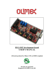
Now you can try another experiment. Connect the PWG to channel 0 of
the ADC and execute the following code segment:
> > > p.set_frequency(1000)
> > > m = p.read_block(100, 50, 0)
> > > p.plot(m)
Figure 3.1 is the plot you would get:
Let's now play with the `multi_read_block' function. The function reads
analog data from multiple channels (remember, the Phoenix ADC has 4
channels) and returns them as a list of the form:
[[ts1, adval0, ... advaln], [ts2, adval0, ... advaln], ......]
where adval0 is value read from channel 0, adval1 is data read from channel
1 and so on. Let's try an experiment. Connect channel 0 of the ADC to
GND and Channel 1 to +5V. Now, execute the following code segment:
26
Figure 3.1: Square wave digitized by ADC
> > > p.add_channel(1)
> > > m = p.multi_read_block(100, 50, 0)
> > > print m
Here are the rst few readings:
[[0, 19.607843137254903, 4960.7843137254904], [50, 0.0, 4980.3921568627447],
[100, 0.0, 4980.3921568627447], [150, 0.0, 4980.3921568627447],
[200, 0.0, 4960.7843137254904]]
Note the time-stamp values increasing in steps of 50 micro seconds while
channel 0 and channel 1 values stay close to 0V and 5V.
How does the multi_read_block function know what all channels have
to be digitized? Code running on the Phoenix box maintains a channel list
which will by default have only channel 0. You can add channels to the
list by calling `add_channel 'and remove channels from the list by calling
`del_channel'. Whenever a multi_read_block is invoked, this channel list
is consulted and analog values on all the channels in the list are digitized.
As an experiment, try deleting one channel from the list and re-issuing the
`multi_read_block' call.
27
Figure 3.2: Rising-to-falling edge delay
The multi_read_block function examines only the channel list - it does
not care which channel has been set by calling select_adc(). The channel list
is maintained internal to the memory of the micro-controller which controls
the Phoenix box - if an application adds a channel to the list, a call to
multi_read_block() later from another application will result in that channel
also getting digitized. Programs like CROs must remove all channels from
the list while starting and then add the required ones.
3.6 Time Measurement Functions
The Phoenix library includes several functions which can be invoked to measure time periods. Most of these functions basically measure time delays
between rising/falling edges on the various Digital Input pins or Analog Comparator Input. Say you wish to compute the on time of a square wave applied
to digital input pin D0 (see gure 3.2); you can simply connect the PWG
socket to D0 and execute:
> > > p.set_frequency(1000)
> > > p.r2ftime(0, 0)
500
The function accepts two digital input pin numbers (which can be the same
or dierent) and returns the time in microseconds between two consecutive
rising and falling edges.
Similarly we can measure the falling edge to rising edge time also using
the 'p.f2rtime(0,0) call. From which we can calculate the period of the wave
and the duty cycle. The arguments can be dierent. For example you can
measure the time between a rising edge on one Input to a rising edge on
another Input.
28
Digital Inputs are specied by argument values from 0 to 3. If the Input
is connected to the Analog Comparator use the argument value '4' as shown
below.
> > > p.r2ftime(4, 4)
500
Time measurement capability is important for many experiments. Direct
measurement of the velocity of sound, period of a pendulum etc. will be
done using this feature. For measuring the time period of a signal applied
to an Input we can use the function 'p.multi_r2rtime(pin, skipcycles)'. The
skip cycles mentions the number of cycles to be skipped in between. If it
is zero, you get the period of the wave. Higher number can be used to get
the eect of averaging. The result of measuring a 1 KHz signal connected to
'Input 0', the result is the time taken for 10 cycles.
> > > p.multi_r2rtime(0,9)
10000
You will nd more information regarding these functions in the API reference.
3.7 Non-programmable units
We have had a brief tour of all the programmable features which the Phoenix
box provides. There are a few functional units within the Phoenix box which
can't be manipulated by code; understanding how these units work is essential for doing practical experiments with Phoenix. In the next part of this
document, we shall look at these non-programmable units.
3.7.1 Converting bipolar signals to unipolar
The ADC channels accept only unipolar signals (0-5V); the Phoenix box
comes with two ampliers which take a bipolar -5V to +5V signal and raises
it to 0 - 5V. Search around the front panel for a section which looks like what
is shown in Figure 3.3
29
OUT
(-X+5)/2
IN
Figure 3.3: Oset amplier
If the input voltage is X, output is (-X + 5)/2. Test this out by applying 0V and 5V at one of the inputs and measuring the voltage at the
corresponding output using a multimeter.
Exercise Test the oset amplier with an input of -5V. You can use the
inverting Op-Amps described in the next section to generate -5V.
3.7.2 Inverting Op-Amps with externally controllable
gain6
In many practical applications, it would be necessary for us to take a very
weak signal (say a few millivolts) and convert it into a `stronger' one which
can be processed by the ADC, Analog comparator or digital inputs. We will
have to amplify the signal hundreds of times. The Phoenix box provides two
inverting ampliers (Figure ??) whose gain (ie, amplication factor) can be
set by connecting an external resistor of appropriate value7 . The value of the
resistor is found using the formula:
Gain = 10KΩ/Ri
6 The
operational ampliers used for implemeting them require both positive and negative supply voltages. Phoenix-M generates them by using a charge pump IC that gives
output from +/- 6V to +/-7V range. Due to this reason ampliers in some units may
saturate at around 4.5 V. You can test this by giving the +5V supply to the inverting
amplier and check the output using a multimeter (insert a 10K gain resistor for unity
gain).
7 The ampliers can also be used for implementing summing junctions and other inverting op-amp circuits.
30
Ri
IN
OUT
Figure 3.4: Inverting Amplier
So, if you want a gain of 10, you will choose a resistor of value Ri = 1K (note
that resistor values are never exact - a 1K resistor will be never exactly 1K so don't expect to get a gain of precisely 10). Connect the resistor between
the two YELLOW sockets, apply input to the GREEN socket marked `IN'
and take output from the BLUE socket marked OUT. Make sure that you
don't choose a gain greater than 40. You can take the output of one amplier
and feed it into the input of another one if you want larger amplication.
The units are implemented by TL084 op-amps and will have some `oset'
- that is, there will be some voltage at the output even when the input is
zero. To measure this, ground the input, supply a gain resistor of 10K Ohm
and measure the output. You should see a value in the range of 1-2 mV. Try
with a gain resistance value of 1KOhm and you will note that it is in the
range of 10-20 mV. You should take this eect in consideration when you are
doing precise measurements.
3.7.3 Non-Inverting variable gain Amplier
There is one Non-Inverting amplier whose gain can be controlled by a pluggin resistor Rg connected between the Yellow socket and ground. The Internal feed back resistor is 10 KOhm and the gain will be 1 + 10000/Rg. This
unit is useful for amplifying the RTD type temperature sensor outputs.
3.7.4 The Constant Current Source Module
Phoenix box has a socket labeled `CCS' - it's a 1mA constant current source.
Connect a 1K resistor between the CCS and ground and measure the voltage
across the resistor - it will be 1V. The current through a circuit should vary
31
as you change the value of the resistance, but a CCS will maintain a constant
ow (in this case, 1 milli ampere). Try to verify this behavior!
The CCS module is useful when measuring temperature using thermistors.
3.8 Plug-in Modules
There is a 16 pin connector on the front side of Phoenix-M. It is meant
for plugging in the LCD display and other additional circuitry as explained
below.
3.8.1 16 character LCD display
3.8.2 High resolution AD/DA card
3.8.3 Radiation detection system
3.9 Other Accessories
For doing experiments using Phoenix we require dierent kinds of sensors.
Sensors for measuring temperature, pressure etc. are commercially available.
Most of them provide a low level voltage output proportional to the measured
parameter. This can be fed to one of the ADC inputs after amplication.
The gain decided in such a way that the maximum output from the sensor
is amplied to the upper limit of the ADC input. For example, if we plan to
measure temperature up to 1000 celcius and the sensor output is 100 mV at
that temperature the gain is selected is 50, to get a maximum 5V at the ADC
input. This is required to utilize the ADC to its maximum resolution. There
are several other sensors and accessories that we can make using available
components.
32
100
L14G1
1K
2N2222
1K
5V
GND
OUT
Figure 3.5: Light barrier circuit
3.9.1 Light barrier
The light barrier is a U shaped structure with a photo-transistor and a Light
Emitting Diode facing each other with a gap of 2 cm in between, as shown in
gure 3.5 . There are three connections to the module, Ground, 5V supply
and the signal output. The output of the module is generally LOW and
goes high when the light emitted by the LED is prevented from reaching the
photo-transistor. By connecting this to Phoenix Digital Input sockets one
can measure time intervals.
3.9.2 Rod Pendulum
3.9.3 Pendulum motion digitizer using DC motor
3.9.4 Temperature Sensors
33
Chapter 4
Experiments
Phoenix-M is a computer interface with some added features. Several experiments on electricity and electronics can be done without much extra
accessories. Science experiments require sensor elements that converts physical parameters into electrical signals. The number of science experiments
one can do with Phoenix-M is limited mainly by the availability of sensor
elements. Here we describe several experiments that can be done using some
sensor elements that are easily available. During the tutorial introduction we
interacted with Phoenix-M by typing commands at Python prompt. Typing
them in a le using a text editor and executing under python makes correcting errors much easier. Here we will follow that approach and all the
programs listed below are available on the Phoenix CD.
4.1 A sine wave for free - Power line pickup
There are two types of electric power available ,generally known as AC and
DC power. The Direct Current or DC ows in the same direction and is
generally made available from battery cells. The electricity coming to our
houses is Alternating Current or AC, which changes the direction of ow
continuously. What is the nature of this direction change. The frequency of
AC power available in India is 50 Hz. Let us explore this using Phoenix-M
and a piece of wire. A frequency of 50 Hz means the period of the wave
34
is 20 milliseconds. If we capture the signal for 100 milliseconds there will
be 5 cycles during that time interval. Let us digitize 200 samples at 500
microsecond intervals and analyze it.
Connect one and of a 25 cm wire to the Ch0 input of the ADC and let the
other end oat. The 50 Hz signals picked up by the ADC can be displayed
as a function of time by the read_block() and plot_data() functions. With
few lines of code you are making a simple CRO !
Type in the following program in a text editor
1
and save it as a le
named say `pickup.py'.
import phm
p = phm.phm()
p.select_adc(0)
while p.read_inputs() == 15:
v = p.read_block(200, 500,1)
p.plot_data(v)
p.save_data(v, 'pickup.dat')
Run the program (by typing `python pickup.py' at the Operating System
command prompt) after plugging one end of 25 cm wire to Ch0 of the ADC.
Make sure that none of the digital input pins are grounded. You should see
a waveform similar to that of gure 4.1. Adjust the position of the wire or
touch the oating end with your hand to see the changes in the waveform.
How do you terminate the program? The `while' loop is continuously
reading from the digital inputs and checking whether the value is 15 - if none
of the sockets D0 to D3 are grounded, the value returned by read_inputs()
will denitely be 15 and the loop body will execute. If you ground one of the
digital inputs, the value returned by read_inputs will be something other
than 15; this will result in the loop terminating. Terminate the program
when a good trace is on the screen, last sample collected is saved to the disk
le 'pickup.dat' just before exiting.
1 if
you are not familiar with standard GNU/Linux editors like vi or emacs, you can use
`Nedit', which is available from the start menu of the Live-CD. Notepad under MSWindows
35
Figure 4.1: Power line Pickup
4.1.1 Mathematical analysis of the data
By counting the number of waves within a given time interval one can roughly
gure out the frequency of the line pickup but it won't be accurate and don't
tell us much about the nature of the wave. Let us approach the problem in a
more systematic manner. We have measured the value of the voltage at 200
dierent instances of time and want to nd out the function that governs the
time dependency of the voltage. Problems of this class are solved by tting
the experimental data with some mathematical formula provided by the theory governing the physical phenomena under investigation. Curve tting is
a method of comparing experimental results with a theoretical model.
Here the theoretical value of voltage as a function of time is given by a
sinusoidal wave represented by the equation V = V0 sin 2πf , where V0 is
the amplitude and f is the frequency. The experimental data can be 'tted'
using this equation to extract these parameters. We use the two dimensional
plotting package xmgrace [2] for plotting a tting the data. Xmgrace is free
software and included on the CD along with user manual and a tutorial.
Xmgrace is started from the command prompt with le 'pickup.dat' , saved
36
4000
Voltage (mV)
2000
0
-2000
-4000
0
20000
40000
60000
Time (usecs)
80000
1e+05
Figure 4.2: Power line pickup and its sine wave t
by the python program, as the argument.
# xmgrace pickup.dat
Select Data− > T ransf ormation− > N onLinearCurveF itting from the
main menu and enter the equation V (t)= V0 sin(2πf t/1000000.0 + θ) + C .
Xmgrace accepts the adjustable parameters as A0, A1 etc.
• V (t) is the value of voltage at time = t
• V0 is the amplitude. The value will be close to 5000 milli volts (represented by parameter A0)
• f is the frequency of the wave (parameter A1)
• t is the value of time, divided by 1000000 to convert micro seconds to
seconds
• θis the phase oset since we are not starting the digitization at zero
crossing (parameter A2)
37
• C is the amplitude oset that may be present (parameter A4)
Reasonable starting values should be given by the user for V0 and f to guide
the tting algorithm. Try dierent values until you get a good t. The gure
4.2 shows the data plotted along with the tted curve. The Curve tting
window 4.3 shows the parameter values.
The extracted value of frequency is 48.73 Hz ! Did not believe it and cross
checked it by feeding a 50 Hz sine wave from a precision function generator
to the ADC input. The result of a similar analysis gave 49.98 Hz. Checked
with the power distribution people and conrmed that the line frequency was
really below 49 Hz.
Exercise: Repeat the experiment by changing the length of the wire,
touching one end by your hand and rising the other hand, moving it near
any electrical equipment etc. (do not touch any power line). You can also
analyze other wave forms if you have a signal generator.
4.2 Capacitor charging and discharging
Every student learning about electricity knows that a capacitor charges and
discharges exponentially but not very many has seen it doing so. Such experiments require fast data acquisition since the entire process is over within
milli seconds. Let us explore this phenomena using Phoenix-M. All you need
is a capacitor and a resistor.
Refer Figure 4.4 on page 40 for the experimental setup. The RC circuit
under study is connected between the Digital output socket D3 and Ground.
The voltage across the capacitor is monitored by the ADC channel 0. The
voltage on D3 can be set to 0V or 5V under software control. Taking D3
to 5V will make the capacitor charge to 5V through the resistor R and then
taking D3 to 0V will cause it to discharge. All we need to do is digitize
the voltage across C just after changing the output of D3. Let us study the
discharge process rst. The python program cap.py listed below does the
job.
import phm, time
38
Figure 4.3: Curve tting window of xmgrace
39
D3
1K
1uF
ADC CH0
Figure 4.4: Circuit to study Capacitor
p = phm.phm()
p.select_adc(0)
p.write_outputs(8)
time.sleep(1)
p.enable_set_low(3)
data = p.read_block(200,50, 0)
p.plot_data(data)
time.sleep(5)
We make the digital output pins go high and sleep for 1 second (allowing
the capacitor to charge to full 5V). The call to function p.enable_set_low(3)
is similar to select_adc() or add_channel() ,whose eect is seen only later,
when a read_block or multi_read_block is called. The idea is this - in
certain situations, an ADC read should begin immediately after a few digital
outputs are set to 1 or 0 - so we can combine the two together and ask
the ADC read functions themselves to do the `set to LOW or HIGH' and
then start reading. In this case, it brings to logic LOW pin D3, thereby
starting the capacitor discharge process. The function then starts reading
the voltage across the capacitor applied on ADC channel 0 at 250 microsecond
intervals2 . The voltage across the capacitor as a function of time is shown
2 You
may wonder as to why such a seemingly complicated function like enable_set_low
is required. We can as well make the digital output pin go high by calling write_outputs
and then call read_block. The problem is that all these functions communicate with
the Phoenix box using a slow-speed serial cable. For example, the read_block function
simply sends a request (which is encoded as a number) over the serial line asking the
micro-controller in the Phoenix box to digitize some input and send it back. By the time
this request reaches the micro-controller over the serial line, the capacitor would have
discharged to a certain extend! So we have to instruct the Phoenix micro-controller in
just ONE command to set a pin LOW and then start the digitization process.
40
Figure 4.5: RC Discharge Plot
in Figure 4.5, which looks like an exponential function. When the rate of
change of something is proportional to its instantaneous value the change is
exponential.
Let us examine why it is exponential and what is an exponential function
with the help of some elementary relationships.
The discharge of the capacitor results in a current I through the resistor
and according to Ohm's law V = IR.
Voltage across the capacitor at any instant is proportional to the stored
charge at that instant, V = Q/C .
These two relations imply I =
of ow of charge, I =
Q
RC
and we current is nothing but the rate
dQ
.
dt
Solving the dierential equation
t
Q
dQ
= RC
dt
t
results in Q(t) = Q0 e− RC which
also implies V (t) = V0 e− RC
Exercise: Modify the python program to watch the charging process.
Change the code to make D3 LOW by calling p.write_outputs(0) and set
it to HIGH just before digitization with p.enable_set_high(3). Extract the
RC value by tting the data using the equation using xmgrace package.
41
CCS
ADC CH0
D3
Figure 4.6: Linear Charging of Capacitor
4.2.1 Linear Charging of a Capacitor
Exponential charging and discharging of capacitors are explained in the previous section. If we can keep the current owing through the resistor constant, the capacitor will charge linearly. Let's wire up the circuit shown in
Figure 4.6 When D3 is HIGH no charging occurs. When D0 goes LOW the
capacitor starts charging through the 1mA constant current source.
and run the following Python script:
import phm, time
p = phm.phm()
p.enable_set_low(3)
p.write_outputs(8)
time.sleep(1)
v = p.multi_read_block(400, 20, 0)
p.plot_data(v)
time.sleep(5)
You will obtain a graph like the one shown in Figure
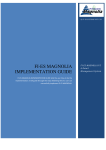
4.3 IV Characteristics of Diodes
Diode IV characteristic can be obtained easily using the DAC and ADC
features. The circuit for this is shown in gure 4.8. Connect one end of a 1
42
Figure 4.7: Linear charging. R = 1 KOhm , C = 1 uF
DAC
Ch0
1K
GND
Figure 4.8: Circuit for Diode IV Characteristic
KOhm resistor to the DAC output. The other end is connected to the ADC
Ch0 Input. Positive terminal of the diode also is connected to the ADC Ch0
and negative to ground. The Voltage across the diode is directly measured
by the ADC and the current is calculated using Ohm's law since the voltage
at both ends of the 1 KOhm resistor is known.
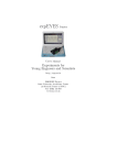
We have tried to study dierent diodes including Light Emitting Diodes
with dierent wavelengths. The code 'iv.py' is ran for each diode and the
output redirected to dierent les. For example; 'python iv.py > red.dat'
after connecting the RED LED. The code 'iv.py' is listed below.
import phm, time
p=phm.phm()
43
5
4148
DR150
4
Current (mA)
RED GREEN YELLOW
3
WHITE
2
1
1.
0
0
500
1000
1500
Voltage (mV)
2000
2500
3000
Figure 4.9: Diode Characteristics
p.set_adc_size(2)
p.set_adc_delay(200)
va = 0.0
while va <= 5000.0:
p.set_voltage(va)
time.sleep(0.001)
vb = p.zero_to_5000()[1]
va = va + 19.6
print vb, ' ' , (va-vb)/1000.0
The program output is redirected to a le and plotted using the program
'xmgrace', by specifying all the data les as command line arguments. The
output is shown in the gure 4.9. Note the dierence between dierent diodes.
If the frequency of the LEDs are known it is possible to estimate the value
of Plank's constant from these results.
4.4 Mathematical operations using RC circuits
RC circuits can be used for integration and dierentiation of waveforms with
respect to time. For example a square-wave of a particular frequency can be
integrated to a triangular wave using proper RC values. In this experiment,
44
PWG
1K
ADC CH0
ADC CH1
1uF
Figure 4.10: Integration circuit
we will apply a square wave (produced by the PWG) to CH0 of the Phoenix
ADC. We will apply the same signal to an RC circuit (R=1K, C=1uF) and
observe the waveform across the capacitor. The circuit is shown in gure
4.10.We will repeat the experiment for 3 dierent cases by varying the Period
of the square wave to show the dierent results.
1. RC ≈T , Results in a Triangular wave form4.11
2. RC > > T, The result is a DC level with some ripple4.12
3. RC < < T, The sharp edges becomes exponential. 4.13
The code 'sqintegrate.py' which generated these three plots is as follows:
"""data was taken with 1K resistor, 1uF capacitor
Three sets are taken:
a) freq=1000 Hz and sampling delay = 10micro seconds, samples=400
b) freq=5000 Hz and sampling delay = 10micro seconds, samples=300
c) freq=100 Hz sampling delay = 20micro seconds, samples=300
"""
import phm
p = phm.phm()
45
Figure 4.11: RC > T
Figure 4.12: RC > > T
Figure 4.13: RC < < T
46
+5V
PWG
1 uF
1K
Piezo
Buzzer
20x
20x
(-X+5)/2
ADC CH0
MIC
Figure 4.14: Microphone digitizing buzzer sound
freq = 1000
samples = 300
delay = 10
p.add_channel(0)
p.add_channel(1)
print p.set_frequency(freq)
while p.read_inputs() == 15:
p.plot_data(p.multi_read_block(samples, delay, 0 ))
Run the code by changing the frequency to study the relation between RC
and T
4.5 Digitizing audio signals using a condenser
microphone
A condenser microphone is wired as shown in gure 4.14to capture the audio
signals. One end of the microphone goes to Vcc through a resistor, the other
end is grounded. The output is taken via a capacitor to block the DC used
for biasing the microphone. The signal is amplied by two variable gain
inverting ampliers in series with a total gain of 400. The amplied output
is level shifted and connected to ADC channel 0. The program 'cro.py' is
47
3000
Volatge (mV)
2000
1000
0
-1000
-2000
0
1000
2000
3000
Time (usecs)
4000
5000
Figure 4.15: Buzzer output digitized
used to capture the waveform and a screen-shot is shown in gure 4.15.
4.5.1 Exercise
The data collected by the program 'cro.py' is in the le 'buzzer.dat' on the
CD. Open it in xmgrace and do a curve tting to extract the frequency as
described in section 4.1. The frequency can be roughly estimated by looking
through the data le for time interval between two zero crossings. Hint:The
value is close to 3.7KHz
The technique of taking Fourier Transforms using Python is discussed in
an Appendix. Go through it and see whether you can calculate the frequency
using that.
4.6 Synchronizing Digitization with External 'Events'
In the previous examples we have seen how to digitize a continuous waveform.
We can start the digitization process at any time and get the results. This
is not the case for transient signals. We have to synchronize the digitization
process with the process that generates the signal. For example, the signal
induced in a coil if you drop a magnet into it. Phoenix-M does this by making
the 'read_block()' and 'multi_read_block()' calls to wait on a transition on
the Digital Inputs or Analog Comparator Input.
48
Connect the condenser microphone as shown in gure. Congure the two
inverting ampliers to give a gain of 20 and 10. (rst plug-in resistor is
500 Ohm and second one is 1 KOhm). The output of the second inverting
amplier is given to Digital Input D3 through a 1K resistor. The same is
given to ADC through the level shifting amplier.
Make some sound to the microphone. The 'p.enable_rising_wait(3)' will
make the read_block() function to wait until D3 goes HIGH. With no input
signal the input to D0 will be near 0V, that is taken as LOW. The program
'wcro.py' used is listed below.
import phm
p = phm.phm()
p.select_adc(0)
p.enable_rising_wait(3)
while 1:
v = p.read_block(200,20,1)
if v != None:
p.plot_data(v)
Exercise: Use a similar setup to study the voltage induced on a coil when
a magnet is suddenly dropped into it.
4.7 Temperature Measurements
In certain experiments it is necessary to measure temperature at regular
time intervals. This can be done by connecting the output of a temperature
sensor to one of the ADC inputs of Phoenix and record the value at regular
intervals. There are several sensors available for measuring temperature,
like thermocouples, platinum resistance elements and solid state devices like
AD590 and LM35. They work on dierent principles and require dierent
kind of signal processing circuits to convert their output into the 0 to 5V
range required by the ADC. We will examine some of the sensors in the
following sections.
49
Figure 4.16: Collision sound.microphone
CCS
PT100
GND
gain = 1+10K/330
+
330
Ch0
GND
Figure 4.17: PT100 Circuit
4.7.1 Temperature of cooling water using PT100
PT100 is an easily available Resistance Temperature Detector , RTD, that
can be used from -2000 C to 8000 C. It has a resistance of 100 Ohms at zero
degree Celsius; the temperature vs resistance charts are available. The circuit
for connecting PT100 with Phoenix-M is shown in gure 4.17
The PT100 sensor is connected between the 1mA Constant Current Source
and ground. The voltage across PT100 is given by Ohm's law, for example
if the resistance is 100Ω the voltage will be 100 * 1 mA = 100 mV. This
must be amplied before giving to the ADC. The gain is chosen in such a
50
way that that amplier output is close to 5V at the maximum temperature
we are planning to measure. In the present experiment we just observe the
cooling curve of hot water in a beaker. The maximum temperature is 1000 C
and the resistance of PT100 is 138Ωat that point that gives 138 mV across
it. We have chosen a gain of roughly 30 to amplify this voltage. The gain is
provided by the non-inverting amplier with a 330Ωresistor from the Yellow
socket to ground.
How do we calculate the temperature from the measured voltage ? The
resistance is easily obtained by dividing the measured voltage by the gain
of the amplier. To get the temperature from the resistance one need the
calibration chart of P100 or use the equation to calculate it.
RT = R0 [1 + AT + BT 2 − 100CT 3 + CT 4 ]
• RT = Resistance at temperature T
• R0 is the resistance at 00 Celsius.
• A = 3.9083 × 10-3
• B = −5.775 × 10-7
The rst three terms are enough for temperatures above zero degree Celsius and the resulting quadratic equation can be solved for T. The program
'pt100.py' listed below prints the temperature at regular intervals. The output of the program is redirected to a le named 'cooling_pt100.dat' and
plotted used xmgrace as shown in gure4.18
import phm, math,
p = phm.phm()
gain = 30.7
offset = 0.0
ccs_current = 1.0
def r2t(r):
r0 = 100.0
A = 3.9083e-3
time
#
#
#
#
amplifier gain
Amplifier offset, measured with input grounded
CCS output 1 mA
Convert resistance to temperature for PT100
51
90
Temp (Celcius)
80
70
60
50
0
500
1000
Time (seconds)
2000
1500
Figure 4.18: PT100. Cooling water temperature
B = -5.7750e-7
c = 1 - r/r0
b4ac = math.sqrt( A*A - 4 * B * c)
t = (-A + b4ac) / (2.0 * B)
return t
def v2r(v):
v = (v + offset)/gain
return v / ccs_current
p.select_adc(0)
p.set_adc_size(2)
p.set_adc_delay(200)
strt = p.zero_to_5000()[0]
for x in range(1000):
res = p.zero_to_5000()
r = v2r(res[1])
temp = r2t(r)
print '%5.2f %5.2f' %(res[0]-strt, temp)
time.sleep(1.0)
Even though the experiment looks simple there are several errors that
need to be eliminated. The CCS is marked as 1 mA but the resistors in the
circuit implemented that can have upto 1% error. To nd out the actual
52
current do the following. Take a 100 Ohm resistor and measure its resistance
'R' with a good multimeter. Connect it from CCS to ground and measure
the voltage 'V' across it. Now V/R gives you the actual current output from
CCS.
For measurements around room temperature the voltage output is under
a couple of hundred millivolts. For better precision this need to be amplied
to 5V, to utilize the full range of the ADC. A gain of 20 to 30, depends
on the upper limit of measurement, can be implemented using the variable
gain ampliers. The oset voltage of the amplier should be measured by
grounding the input and subtracted from the actual readings. The actual
gain should also should be calculated by measuring the input and output at
a a couple of voltages.
Another method of calibrating the setup is to measure the ADC output
at 00 and1000 and assume a linear relation, which may not be very accurate,
between the ADC output and the temperature.
4.8 Measuring Velocity of sound
The simplest way to measure the velocity of anything is to divide the distance
s by time taken. Since phoenix can measure time intervals with microsecond
accuracy we can apply the same method to measure the velocity of sound.
We will rst try to do this with a pair of piezo electric crystals and later by
using a microphone.
4.8.1 Piezo transceiver
A piezo electric crystal has mechanical and electrical axes. It deforms along
the mechanical axis if a voltage is applied along the electrical axis. If a force
is applied along the mechanical axis a voltage is generated along the electrical
axis. We are using a commercially available piezo transmitter and receiver
pair that has a resonant frequency of 40 KHz. The experimental setup is
shown in gure 4.19.
The transmitter piezo is excited by sending a 13 micro seconds wide pulse
53
100 Ohm 100x
Digout D3
Tx
GND
Rx
Digin D3
1K
GND 100 Ohm 100x
Figure 4.19: Piezo Transceiver setup measuring velocity of sound
Distance (cm)
4
5
6
7
Timeusec)
224
253
282
310
Dist. dierence
Time di.
Vel. (m/s
1
2
3
29
58
86
344.8
344.8
348.8
Table 4.1: Velocity of sound
on Digital Output Socket D3 to generate a sound wave. The sound wave
reaches the receiver piezo kept several centimeters away and induces a small
voltage across it. This signal is amplied by two variable gain ampliers in
series, each with a gain of 100. The output is fed to Digital Input D3 through
a 1K resistor3 . The interval between the output pulse and the rising edge of
D3 is measured by the following program 'piezo.py'. The output is redirected
to a le
import phm
p=phm.phm()
p.write_outputs(0)
for x in range(10):
print p.pulse2rtime(3,3,13,0)
To avoid gross errors in this experiment one should be aware of the following. Applying one pulse to the transmitter piezo is like banging a metal plate
3 It
is very important to use this resistor. The amplier output is bipolar and goes
negative values. Feeding negative voltage to D3 may damage the micro-controller. The
1KOhm resistor acts as a current limiter for the diode that protects the micro-controller
from negative inputs.
54
to make sound, it generates a train of waves whose frequency is around 40
KHz. The receiver output is a wave envelope whose amplitude rises quickly
and then goes down rather slowly. When we amplify this signal one of the
crests during the building up of the envelope makes the Digital Input HIGH.
When we increase the distance between the crystals the amplitude of the
signal also goes down. At some point this will result in sudden jump of 25
microseconds in the time measurement which is caused by D3 going HIGH by
the next pulse. This can be avoided by taking groups of reading at dierent
distances varying it by 3 to 4 centi meters.
4.8.2 Condenser microphone
Velocity of sound can be measured by banging two metal plates together and
recording the time of arrival of sound at a microphone kept at a distance.
One metallic plate is connected to ground, another one is connected to a
digital input say D0. The generated sound travels through air and reaches
the microphone and induces an electrical signal. The electrical signal is
amplied 200 times by two ampliers in series and connected to D3. The
experimental setup is shown gure 4.20. We have used 1 mm thick aluminium
plates to generate the sound. When we strike one by the other, the digital
input D0 gets grounded resulting in a falling edge at D0. The amplied
sound signal causes a rising edge on D1 4 . The software measures the time
interval between two falling edges using the following lines of code. To get
better results repeat the measurement several times and take average.
import pm
p = phm.phm()
print p.f2ftime(0,1)
Here is a table of measurements obtained experimentally:
4 Rising
or falling edge depends on the amplier oset etc. If the amplier output will
start oscillating when the sound signal arrives. If is already HIGH it will go LOW when
the sound signal arrives and we should look for a falling edge.
55
Grounded Plate
Digital input D0
5V
1K
distance
Mic
Digital Input D1
1uF 20x
1K
10x
GND
Figure 4.20: Velocity of sound by microphone
Distance (cm)
Time (milli seconds)
Speed = distance/time
0
0.060
To be treated as oset
10
0.350
344.8
20
0.645
341.8
30
0.925
346.8
40
1.218
345.4
50
1517
343.1
60
1810
342.8
4.9 Study of Pendulum
Studying the oscillations of a pendulum is part of any elementary physics
course. Since the time period of a pendulum is a function of acceleration
due to gravity, one can calculate g by doing a pendulum experiment. The
accuracy of the result depends mainly on how accurate we can measure the
period T of the pendulum. Let us explore the pendulum using phoenix.
56
4.9.1 A Rod Pendulum - measuring acceleration due to
gravity
A rod pendulum is very easy to fabricate. We took a cylindrical rod and xed
a knife edge at one end of it to make a T shaped structure. The pendulum is
suspended on the knife edges and its lower end intercepts a light barrier while
oscillating. The light barrier is made of an LED and photo transistor. The
output of the light barrier is connected to Digital Input D3. The program
'rodpend.py' is used for measuring T and calculating the value of g . The
code is listed below.
import phm, math
p=phm.phm()
length = 14.65
# length of the rod pendulum
pisqr = math.pi * math.pi
for i in range(50):
T = p.pendulum_period(3)/1000000.0
g = 4.0 * pisqr * 2.0 * length / (3.0 * T * T)
print i, ' ',T, ' ', g
The output of the program is redirected to a le and a histogram is made
using 'xmgrace' program as shown in gure 4.21. The mean value and percentage error in the measurement can be obtained from the width of the
histogram peak.
4.9.2 Nature of oscillations of the pendulum
A simple pendulum can be studied in several dierent ways depending on the
sensor you have got. If you have an angle encoder the angular displacement
of the pendulum can be measured as a function of time. What we used is
a DC motor with the pendulum attached to its shaft. When the pendulum
oscillates it rotates the axis of the motor and a small time varying voltage
is induced across the terminal of the motor. This voltage is amplied and
57
20
frequency
15
10
5
0
979
979.5
980
gravity ’g’
981
980.5
Figure 4.21: Measured 'g'. Histogram
plotted as a function of time. The experimental setup and output are shown
in gure 4.22 on the facing page. The program pend_digitize.py is listed
below.
The output of the program is send to a le and plotted using xmgrace.
The period of oscillation can be extracted by tting the data with the equation of an exponentially decaying sinusoidal wave. The equation used for
tting the data is the following.
A(t) = A0 sin(ωt + θ)e-dt + C
• A(t) - Displacement at time t
• A0 - Maximum displacement
• ω - Angular velocity
• θ - displacement at t=0
• d - Damping factor
• C - Constant to take care of DC oset from ampliers
The angular velocity ω is found to be 7.87 and the length of the pendulum is
15.7 cm. The calculated value of 'g' using the simple pendulum equation ω 2 L
= 972 cm/sec2 . The errors are due to the simple pendulum approaximation
and the error in measurement of length.
58
DC Motor
200x
(X+5)/2
CH0
GND
Pendulum
Figure 4.22: Pendulum block diagram
4000
Voltage (mV)
2000
0
-2000
-4000
0
2
4
Time (sec)
6
8
10
Figure 4.23: Decaying oscillations
59
60
Figure 4.24: Pendulum Data tted with equation
COIL
GND
D0 (output)
D0(Input)
Ion
ball
Contact sensor
Figure 4.25: Gravity by free fall
4.9.3 Acceleration due to gravity by time of ight method
There are many ways to time the free fall of an object under gravity - here is
one interesting idea. Take a small relay and remove its cover so that you can
access the coil directly. Connect one end of the coil to the Digital Output
D0 ( the only output with transistor buering). We have used the coil from
12V relay with a coil resistance of 150 Ohms. The coil resistance should not
be less than 100 Ohms and it should be able to magnetically hold a metal
ball of radius around 1 cm. The experimental setup is shown in gure 4.25.
Digital Output D0 is made high to energize the coil. Now attach the metal
ball to the relay and and release it under software control. The ball falls on
the contact sensor and takes the Input D0 to LOW. The code 'gdirect.py' is
listed below.
import phm, time
p=phm.phm()
p.write_outputs(1)
# energize the coil
time.sleep(2)
# time to attach the ball to the coil
print p.clr2ftime(0,0)# time of flight
The value of gravity g can be calculated using the expression S = 12 gt2 where
S is the distance and t is the time of ight. There are certain sources of error
in this experiment. We assume that the ball is released at the moment the
61
current is withdrawn but due the inductance of the coil the balls falls after a
delay. This delay error can be estimated by taking the readings at dierent
heights. Using two light barriers at dierent hieghts is another solution.
4.10 Study of Timer and Delay circuits using
555 IC
Constructing astable and monostable multi-vibrators using IC555 is done
in elementary electronics practicals. Using phoenix one can measure the
frequency and duty-cycle of the output with micro second accuracy. In the
case of mono-stable Phoenix can apply the trigger pulse and measure the
width of the output.
4.10.1 Timer using 555
An astable multi-vibrator is wired using IC 555 as shown in gure 4.26. The
output of the circuit is fed to CNTR input for frequency measurement and
then to Digital Input D0 for duty cycle measurement. The code used is
shown below along with the results obtained at each step.
print p.measure_frequency()
904
print p.r2ftime(0,0)
733
print p.f2rtime(0,0)
371
# signal connected to CNTR
# signal to D0 input
Exercise: Cross check the above results with that predicted by the equation for frequency and duty cycle. The resistor values used are of 1% tolerance
and capacitor of 5% tolerance.
62
5V
4
8
4K7
7
3
IC 555
D0 (input)
6
4K7
2
0.1uF
5
0.01uF
1
Figure 4.26: 555 oscillator circuit
4.10.2 Mono-stable multi-vibrator
The monostable circuit is wired up as shown in gure4.27 . The 555 IC
require a LOW TRUE signal at pin 2 to trigger it. The output goes HIGH
for a duration decided by the R and C values and comes back to LOW.
The following lines of code is used for triggering 555 and measuring the time
interval from trigger to the falling edge of the signal from pin 3.
p.write_outputs(8)
p.pulse2ftime(3,0,1,1)
123
# keep D3 high
# 1 usec wide LOW TRUE pulse on D3 to a falling edge
Again it is left as an exercise to the reader to verify whether 123 microseconds
is acceptable based on the RC values used.
63
5V
4
10K
7
8
3
IC 555
D3 (output)
6
0.01uF
2
D3
Input
5
1
0.1uF
Figure 4.27: Monostable multi-vibrator using 555
64
Chapter 5
Micro-controller development
system
The heart of Phoenix-M hardware is an ATmega16 micro-controller. The
system comes with a pre-loaded program that listens for commands from
the PC through the Serial Port. This program is developed using the same
hardware setup and the AVR GCC compiler. The program is compiled on the
PC and the executable output is uploaded to the micro-controller through
a cable connected to the Parallel port of PC. The AVR GCC compiler for
both GNU/Linux and MS-Windows is provided on the Phoenix CD . Most of
the ATmega16 micro-controller Input/Output pins are available through the
front panel sockets. A 16 Character LCD Display is provided along with C
routines to access it. An introduction to ATmega16 micro-controller is given
below. For more details refer to the PDF document on the CD.
Features
High-performance, Low-power AVR 8-bit Micro-controller
Advanced RISC Architecture
- 131 Powerful Instructions - Most Single Clock Cycle Execution
- 32 x 8 General Purpose Working Registers
- Up to 6 MIPS Throughput at 16MHz
- Fully Static Operation
- On-chip 2-cycle Multiplier
65
Nonvolatile Program and Data Memories
- 16k Bytes of In-System Self-Programmable Flash
- Optional Boot Code Section with Independent Lock Bits
- 512K Bytes EEPROM
- Programming Lock for Software Security
JTAG (IEEE std. 1149.1 Compliant) Interface
- Boundary-scan Capabilities According to the JTAG Standard
- Extensive On-chip Debug Support
- Programming of Flash, EEPROM, Fuses, and Lock Bits through the
JAGS
Interface
Peripheral Features
- On-chip Analog Comparator
- Programmable Watchdog Timer with Separate On-chip Oscillator
- Master/Slave SPI Serial Interface
- Two 8-bit Timer/Counters with Separate Prescalar, Compare
- One 16-bit TImer/Counter with Separate Prescaler, Compare and Capture mode
- Real TIme Counter with Separate Oscillator
- Four PWM Channels
- 8-channel, 10-bit ADC
- Byte-oriented Two-wire Serial Interface
- Programmable Serial USART
Special Micro-controller Features
- Power-on Reset and Programmable Brown-out Detection
- Internal Calibrated RC Oscillator
- External and Internal Interrupt Sources
- Six Sleep Modes: Idle, ADC Noise Reduction, Power-save, Power-down,
Standby, and Extended Standby
I/O and Packages
- 32 Programmable I/O Lines
- 40-pin PDIP, 44-lead TQFP, and 44-pad MLF
Operating Voltages
66
Figure 5.1: ATmega16 . Pin diagram and DIP package
- 4.5-5.5V for ATmega16
Speed Grades
- 0-16 MHz for ATmega16
Power Consumption at 4 Mhz, 3V, 35 ◦ C
- Active: 1.1mA
- Idle Mode: 0.35mA
- Power-down Mode: < 1 µA
5.1 Hardware Basics
ATmega16 interacts with the external world through four I/O ports, named
as A,B,C and D. The ports are 8 bit wide and each bit can be congured as
input or output. The behavior of the ports are controlled by programming
the corresponding internal registers. In addition to the normal digital Input/Output operation, most of the pins have alternate functions as shown in
67
gure 5.1. Once the alternate functions are enabled internally, corresponding PIN will get connected to those units. For example enabling the on-chip
ADC will make Port A pins as ADC inputs. We will try to introduce the
dierent features of ATmega16 by small example programs. For more details
refer to the ATmega16 manual provided on the CD. Refer to the schematic
diagram5.2 to nd out the wiring between the front panel sockets and ATmega8.
5.1.1 Programming tools
The AVR GCC compiler and associated tools are on the CD. It is desirable
to start with the Live CD rst, where all the programs are installed and
ready to use. On GNU/Linux systems install the 'rpm' les using the script
'install.sh' in the RPM directory. The directory /opt/cdk4avr/bin should be
added to the path for the tools to work properly. Under MS-Windows run
the le W inAV R − install.exe to install the compiler and tools. To save
typing the necessary commands are put in a le named 'compile.bat' 1 . This
script can be used for compiling the code and generate the executable format
le.
echo "compiling $1.c"
avr-gcc -Wall -O2 -mmcu=atmega16 -Wl,-Map,$1.map -o $1 $1.c
avr-objcopy -j .text -j .data -O ihex $1 $1.hex
avr-objdump -S $1 > $1.lst
More information on the AVR GCC compiler and the library functions are
on the CD in 'html' format.
5.1.2 Setting Clock Speed by Programming Fuses
Several parameters like processor clock source, clock speed etc. can be programmed through the same cable that is used for uploading the executable
1 The
.bat extension may look odd but there is a reason. With that extension it can be
used under MSWindows also.
68
Figure 5.2: Phoenix-M Hardware schematics
69
6pin con. pin #
1
2
3
4
5,6
Signal
RESET
SCK
MISO
MOSI
GROUND
AT pin #
9
8
7
6
11
P.Port pin #
16
1
11
2
19
Table 5.1: Parallel port programming cable
code. To set 8MHz clock speed with external crystal and disable the JTAG
interface, set the fuse LOW to EF and HIGH to D9.
uisp -dprog=dapa -dpart=atmega16 -dlpt=0x378 --wr_fuse_l=0xEF
uisp -dprog=dapa -dpart=atmega16 -dlpt=0x378 --wr_fuse_h=0xD9
The Phoenix-M programs are written for 8MHz clock speed. The RS232
baud rates are derived from the processor clock and it is 38400 baud for
8MHz clock. The Python library uses this speed and the processor MUST
be set to 8MHz for things to work . Refer to the ATmega16 documentation
for more details.
5.1.3 Uploading the HEX le
The executable le is generated in the HEX format. It is uploaded to ATmega16 through the PC parallel port using the cable provided. The pin
connections of the cable are shown in table5.1. One end of the cable is a 6
pin connector and other end is 25 pin D connector for the PC parallel port.
A program named uisp is used for uploading the HEX le. The same
program is used for setting the fuses of ATmega16. The script 'load.bat' ,
listed below, contains the commands to upload a le. The usage of this is
explained in the examples section.
echo "Uploading $1.c"
uisp -dprog=dapa -dpart=atmega16 -dlpt=0x378 --erase
uisp --verify -dprog=dapa -dpart=atmega16 -dlpt=0x378 --upload if=$1.hex
70
For example, executing the following command from the directory where
'load.bat' and '.hex' are located will upload 'avrk.hex' to the micro-controller.
# ./load.bat avrk
Uploading this program is necessary for the python library to communicate
to Atmega8. After trying any of the following examples load avrk if you
want to restore the functioning of Phoenix-M as a PC interface.
5.2 Example Programs
The example programs will use Phoenix-M hardware for demonstrating various features of ATmega16. Extra hardware will be plugged into the front
panel sockets as required. It is desirable to have a multimeter to test the
results.
5.2.1 Blinking Lights
If you have booted from the live CD, open a command prompt and set
the default directory as 'root/phm'. Create a le named 'blink.c' with the
following lines in it. Connect an LED from the socket marked ADC Ch0 to
ground through a 1KOhm resistor.
#include <stdio.h>
#include <stdlib.h>
#include <inttypes.h>
#include <avr/io.h>
void delay (uint16_t k) // roughly 2 usec per loop at 8 MHz system clock
{
volatile uint16_t x = k;
while (x) --x;
}
int main (void)
{
71
DDRA = 0xff;
// Configure all bits of PORT A as output
for(;;)
{
PORTA = 255;
delay(20000);
PORTA = 0;
delay(20000);
}
}
Compile the code and upload it to ATmega8 using the scripts as shown below;
# ./compile.bat blink
# ./load.bat blink
Now the LED should start blinking. What is happening? How our ADC
input became an output ? . The program blink.c has congured the PORT
A as an output port and we have not enabled the ADC. All the four ports
can be congured as input or output in a similar fashion.
5.2.2 Writing to the LCD Display
Phoenix-M has a provision to attach a 16 character LCD display to the board.
We have used the Hitachi 44780 based LCD display that is available easily.
The connections between the LCD module and ATmega16 are shown in the
table5.2 . There are total seven connections between LCD and ATmega16,
four of them are data lines and three are control lines.
Programming details of the LCD module and the example programs are
available on given on the CD. We will use the le lcd16.c from the cprog
directory. A program named lcdtest.c also is given in the same directory.
Here is a small program hello.c that writes to the LCD display. LCD Display
was the main debugging tool during Phoenix-M program development.
#include <stdio.h>
#include <stdlib.h>
72
Pin
1
2
3
4
5
6
7
8
9
10
11
12
13
14
15
16
Function
Vss
Vdd
V0
RS
R/W
EN
DB0
DB1
DB2
DB3
DB4
DB5
DB6
DB7
x
x
Description
Ground pin
+5V supply
Intensity, 0V for maximum
HIGH for Data, LOW for Commands
H for read, L for write
Enable signal
Back light LED control, not used
Table 5.2: LCD connections
#include <inttypes.h>
#include <avr/io.h>
#include "lcd16.c"
int main (void)
{
DDRA = 255;
// PORT A as output
DDRD = 255;
// PORT D as output
initDisplay ();
writeLCD('H');
writeLCD('e');
writeLCD('l');
writeLCD('l');
writeLCD('o');
}
73
ATmega8 Pin
PD4
PD3
PD2
PA4
PA5
PA6
PA7
5.2.3 Analog to Digital Converters
The on-chip 10 bit ADC has 8 multiplexed inputs. ATmega16 has analog
supply volatge pin AVCC and an external ADC reference voltage pin. Internal reference voltage source also has been provided. T. Phoenix-M circuit
gives same 5V DC to both AVCC and AREF. Operation of the ADC is controlled through the special registers provided for that purpose. ADCSRA,
ADMUX, ADCL, ADCH etc are the important registers to control the ADC.
Let us explore the ADC functioning using the program adc.c listed below,
which reads the input of channel 0 and writes the digital output to the LCD
display.
#include <stdio.h>
#include <inttypes.h>
#include <avr/sfr_defs.h>
#include <avr/io.h>
#include "lcd16.c"
uint8_t lo, hi;
uint16_t dat;
// 16 bit unsigned datatype
int main()
{
DDRA = 0xf0;
// 4 bits ADC Input + 4 bits LCD data output
DDRD = 255;
// PORTD as output
for(;;)
{
initDisplay();
ADMUX = 0; // External reference, 10 bit data, channel 0
ADCSRA = BV(ADEN) | BV(ADSC) | 7;
// Enable, Start, Low clock speed
while ( !(ADCSRA & (1< <ADIF)) ) ; // wait for ADC conversion
lo = ADCL;
hi = ADCH;
sbi(ADCSRA, ADIF);
// get ready for next conversion
dat = (hi < < 8) | lo;
write16(dat);
74
delay(10000);
}
}
5.2.4 Pulse width modulation using Timer/Counters
ATmega16 has three Timer/Counter units, two of them are 8 bit and one is
16 bit. For a quick demo let us generate a 31.25 KHz pulse on OC2 (pin #
21). For this we program the control register and set point registers of TC2
as shown in the code pwm.c below.
#include <avr/sfr_defs.h>
#include <avr/io.h>
int main()
{
DDRD = 255;
OCR2 = 127; // Change this from 0 to 255 for changing duty cycle
TCCR2 = BV(WGM21) | BV(WGM20) | BV(COM21) | 1; // Fast PWM mode
TCNT2 = 0;
}
Timer/Counters are very versatile and programming them could become really complex depending on the application. Read the documentation for
more details.
75
Chapter 6
Building Standalone Systems
The Phoenix-M hardware can be converted into standalone systems that
can be used independent of the PC. The LCD panel provides a minimalistic
display device. The front panel sockets can be congured for Input/Output
of various kinds. The concept is demonstrated with the following examples.
6.1 Frequency Counter for 5V square wave signal
The CNTR socket is connected to PB0 (T0). We will congure Timer/Counter
0 to count the external pulses applied to this pin and count the number of
pulses for one second. The 16 bit Timer/Counter TC1 will be programmed
to run on a 1 MHz clock generated internally to generate a signal when we
reach one second. The result is displayed on the LCD panel. The program
'frcount.c' is listed below.
#include
#include
#include
#include
#include
#include
<stdio.h>
<stdlib.h>
<inttypes.h>
<avr/sfr_defs.h>
<avr/io.h>
"lcd16.c"
76
uint32_t x;
uint16_t tmp16;
uint8_t tmp8;
char ss[20];
int main()
{
DDRA = 0xf0;
// 4 bits ADC Input + 4 bits LCD data output
DDRB = 0x00;
// Configure as input
PORTB = 255;
DDRC = 0xf0;
// Low nibble Input & High nibble output
PORTC = 15;
// Enable pullup resistors (low 4)
DDRD = 255;
// PORTD as output
// Three lines of code below generates a 31.25 KHz pulse on PWG.
// Connect PWG to CNTR for testing the standalone frequency meter
OCR2 = 127; // Change this from 0 to 255 for changing duty cycle
TCCR2 = BV(WGM21) | BV(WGM20) | BV(COM21) | 1;
// Fast PWM mode
TCNT2 = 0;
// Frequency counter code starts here
while (1)
{
TCCR1B = BV(WGM12) | BV(CS11);// Wavegen mode, Clock/8 to TCC1
TCCR0 = 7;
// normal, External clock
TIFR = 255;
// clear all flags
OCR1A = 49999;
tmp16 = 0;
tmp8 = 0;
TCNT0 = 0;
// counts external input
TCNT1 = 0;
// to keep time with clk/8
while(1)
{
if(TIFR & BV(OCF1A))
// 50000 usecs elapsed
{
if (++tmp8 == 20)
77
{
TCCR0 = 0;
break;
}
TIFR |= BV(OCF1A);
}
// 1 second. Stop counting
if(TIFR & BV(TOV0))
// overflow after 255 counts
{
++tmp16;
TIFR |= BV(TOV0);
// Clear OVF flag
}
}
x = tmp16;
x = (x < < 8) | TCNT0;
sprintf(ss,"%ld",x);
initDisplay();
tmp8 = 0;
while(ss[tmp8]) writeLCD(ss[tmp8++]);
delay(20000);
}
}
The above program also generates a 31.25 KHz square wave on PWG (pin 21
of ATmega8) that can be used for quick testing of the system. The following
table gives the values measured by this program for dierent frequency inputs
from a HP33120A function generator.
78
Frequency from HP33120A
displayed by ATmega8 program
50
50
100
100
1000
1000
5000
4999
10000
9999
50000
49992
100000
99983
500000
4999913
1000000
999828
For counting small amplitude signals amplify them using the gain blocks
provided on Phoenix and feed to the CNTR input through a 1KOhm resistor
in series.
6.2 Room Temperature Monitor
We use the LM35 temperature sensor along with phoenix-M to display the
room temperature on the LCD display. LM35 is a three pin IC with 5V
supply, Ground and the output leads. The output voltage is zero at 0 degree
Celsius and increases 10mV per degree. The output of LM35 is amplied by
the non-inverting amplier. A 1K resistor is used to get a gain of 11. The
amplier output is fed to ADC Ch0. The program 'lm35.c' listed below is
uploaded to the system.
#include
#include
#include
#include
#include
#include
int gain
uint16_t
uint8_t
<stdio.h>
<stdlib.h>
<inttypes.h>
<avr/sfr_defs.h>
<avr/io.h>
"lcd16.c"
= 11;
// amplifier gain is 11 for 1K resistor
tmp16;
tmp8;
79
uint32_t x,y;
char
ss[20];
int main()
{
DDRA = 0xf0;
// 4 bits ADC Input + 4 bits LCD data
DDRB = 0x00;
// Configure as input
PORTB = 255;
DDRC = 0xf0;
// Low nibble Input & High nibble output
PORTC = 15;
// Enable pullup resistors (low 4)
DDRD = 255;
// PORTD as output
ADMUX = 0;
// 10 bit data, channel 0
while (1)
{
ADMUX = 0;
// 10 bit data, channel 0
ADCSRA = BV(ADEN) | BV(ADSC) | 7;
// Low clock speed
while ( !(ADCSRA & (1< <ADIF)) ) ;
// wait for ADC conversio
tmp8 = ADCL;
tmp16 = (ADCH < < 8) | tmp8;
sbi(ADCSRA, ADIF);
x = tmp16;
x = x * 5000;
x = x/1023/gain;
y = x;
x = x / 10;
sprintf(ss,"%ld.%ld",x,y-(x*10));
initDisplay();
tmp8 = 0;
while(ss[tmp8]) writeLCD(ss[tmp8++]);
delay(32000);
}
}
80
Floating point calculations are avoided. Loading the oating point library
will make the size of the executable beyond 16 kilo bytes.
6.2.1 Exercise
Modify the above system to make a temperature controller. Pin #26 (PC4)
of ATmega8 is transistor buered on the phoenix board. This can be used
for driving a 5V relay that in turn will switch the heater power On or OFF.
The state of PC4 can be controlled by software depending on the dierence
between the measured temperature and the reference point.
81
Chapter 7
Appendix A - Number systems
A basic understanding of binary and hexadecimal number systems is required
to work with Phoenix-M.
The Binary Number System
Only two digits, 1 and 0 are available for counting in binary; here is how you
do it: 00, 01, 10, 11, 100, 101, 110, 111, 1000, .... and so on.
Converting a binary number to decimal is simple. Let's convert 1011 to
decimal:
1 ∗ 20 + 1 ∗ 21 + 0 ∗ 22 + 1 ∗ 23
Take each digit of the binary number (from the rightmost one) and keep
multiplying it with increasing powers of 2. Converting small decimal numbers
to binary becomes quite easy with practice - simply visualize this sequence:
.... 128
64
32
16
8
4
2
1
Say you want to convert 37 to binary; 37 is 32 + 4 + 1, so you visualize a
bit pattern
0
0
1
0
0
1
0 1
82
with 1's at positions occupied by 32, 4 and 1 and zero's at all other places.
The rightmost bit (the so called `least signicant bit') of an eight bit
pattern will be labeled D0 and the leftmost bit (the most signicant bit) will
be labeled D7.
The Hexadecimal Number System
Counting
You count in decimal like this: 0, 1, 2, .... 8, 9, 10, 11, 12 ..... There are
only ten distinct symbols from 0 to 9 available. In hexadecimal, you have
16 distinct symbols - you count in hex like this: 0, 1, 2, ....8, 9, A, B, C, D,
E, F, 10, 11, .... 18, 19, 1A, 1B, 1C, 1D, 1E, 1F, 20, ....... The symbol A
represents 10 in decimal, symbol B represents 11 and so on.
Conversion to decimal
It's very easy to convert a hexadecimal number to decimal; let's take the hex
number 12 as an example. The procedure is:
2 ∗ 160 + 1 ∗ 161
The result is 18, which is the equivalent decimal number. One more example
would make things clear. Let's convert the number 2ab3 to decimal. The
procedure is:
3 ∗ 160 + 11 ∗ 161 + 10 ∗ 162 + 2 ∗ 163
We are simply taking each digit of the number from the least signicant
(rightmost) to the most signicant, converting it to decimal and multiplying
it by increasing powers of 16.
83
Conversion to binary
Lets convert the hex number 2A to binary - the idea is to take each hex digit
and convert it into a 4 bit binary number and append all the 4 bit sequences
obtained.
The number A in hex is 10 in decimal - the equivalent binary is 1010.
The number 2 in binary is 0010. So 2A is:
00101010
The reverse conversion (binary to hex) too is simple - group the binary number into 4 bit sequences, convert each 4 bit sequence to hex and append all
the hex digits together.
84
Chapter 8
Appendix B - Introduction to
Python Language
After booting your machine with the Live-CD and logging in as `root' (as
per the instructions provided on the boot up screen), you should familiarize
yourself with the Python programming language as it will be your primary
vehicle for interacting with the Phoenix box.
Arithmetic
Python (http://www.python.org) is a very high level language with clear
syntax and predictable behavior (unlike `C', which never works the way you
imagine it to work!). You can start interacting with it by invoking the command:
python
at the interpreter prompt. You would see something similar to this:
[root@don user-manual]# python
Python 2.3.4 (#1, Sep 11 2004, 22:35:14)
[GCC 3.3.2 20031022 (Red Hat Linux 3.3.2-1)] on linux2
Type "help", "copyright", "credits" or "license" for more information.
>>>
85
The > > > sequence represents the Python `prompt' where you can interactively enter short Python programs. Let's try out our rst program:
> > > print 1+2
3
> > > 1+2
3
> > > print "hello,world"
hello,world
>>>
That's about as simple as you can get1 ! You can do all standard math
operations:
>>> 2 * 3
6
> > > 2 ** 3
8
> > > 2 ** 50L
1125899906842624L
>>> 1 / 2
0
> > > 1/2.0
0.5
>>>
Note that adding a sux `L' converts the number to a `long' integer which
can have as many digits as can be computed within the constraints of time
and space.
It's possible to represent integer constants in three separate bases - decimal (default), octal and hexadecimal.
1 Be
careful not to insert any additional space before the rst character of each line you
type at the prompt! Python has some unusual interpretations for whitespace which may
bewilder a newbie.
86
> > > 0x10
16
> > > 010
8
> > > hex(255)
'0x'
> > > oct(8)
'010'
>>>
The `0x' prex stands for hexadecimal and a simple `0' prex makes the
constant an octal constant.
The dynamic nature of Python
Let's look at a few lines of Python code:
> > > a=1
> > > type(a)
<type 'int'>
> > > a='hello'
> > > type(a)
<type 'str'>
Python does not have any kind of variable declaration, unlike C/C++. A
Python variable is created when an assignment statement is executed. So, the
variable `a' is created only when the statement `a=1' executes - the interpreter
assigns the type `int' to `a' at that point of time. Later, `a' can be assigned
to an object of an entirely dierent type (as in the example above).
Strings
A Python string is a sequence of characters written within single or double
quotations.
87
> > > a= 'hello'
> > > b = 'world'
> > > print a[0]
'h'
> > > print a[-1]
'o'
> > > print a+b
'helloworld'
> > > print a * 3
'hellohellohello'
The manipulations done above are very simple. You can extract individual
characters of a string by `indexing' it - the rst index starts at `0'. It is
possible to do `negative indexing' which helps you extract elements from
right to left. The addition and multiplication operations behave logically.
Let's try another experiment:
> > > str(123)
'123'
> > > str(1.23)
'1.23'
>>>
The `str' functions converts an integer to string. We will nd this useful when
we wish to concatenate an integer or oating point number and a string.
Let's nd out the ASCII value of a character:
> > > ord('A')
65
> > > ord('a')
97
>>>
And let's convert an ASCII value into its equivalent character form:
88
> > > chr(65)
'A'
> > > chr(97)
'a'
>>>
Complex Numbers
Python has built-in complex numbers. Here are a few statements which
demonstrates this capability:
> > > a = (1 + 2j)
> > > b = (3 + 4j)
>>> a + b
4 + 6j
>>> a * b
-5 + 10j
>>>
Arrays (Lists)
Here is how you go about manipulating a set of numbers (or any other objects) in Python:
> > > a = [1,2,3.9,"hello]
> > > a[0]
1
> > > print a[3]
hello
> > > a[4]
Traceback (most recent call last)
File "<stdin>", line 1, in ?
IndexError: list index out of range
89
The expression `a[0]' is said to `index' the array with 0, the rst index. Note
that it is not possible to index the array with 4 as the last element is at index
3; the Python interpreter generates what is called an `exception' if you try
doing it. This is standard behaviour.
You can concatenate arrays, and do more interesting stu:
> > > a = [1, 2, 3]
> > > b = [4, 5, 6]
>>> a + b
[1, 2, 3, 4, 5, 6]
>>> a * 3
[1, 2, 3, 1, 2, 3, 1, 2, 3]
> > > a.append(10)
> > > print a
[1, 2, 3, 10]
> > > print a[0:3] # from index 0 to index 2
[1, 2, 3]
> > > print a[-1] # negative indexing
10
> > > a = range(10)
> > > print a
[0, 1, 2, 3, 4, 5, 6, 7, 8, 9]
>>>
The `#' sign is the comment symbol in Python; comment lines are ignored
by the language interpreter and are written for readability's sake.
Tuples
Tuples are like lists, but with a major dierence. You can't modify the
contents of a tuple in any way.
> > > a=(1,2,3) # a sequence of objects within ordinary parenthesis forms a tuple
> > >a[0] = 9 #error
90
Functions
Here is how you dene a function in Python:
> > > def sqr(x): # note the `colon'
...
return x*x
. . .
>>>
The `...' character sequence (which appears automatically only if you are in
the interactive mode) denotes the fact that you are now within a function
denition. Python syntax says that body of a function should be `indented'
- I have used a `tab' for this purpose2 . We have dened a simple function
`sqr' which accepts a number3 and returns it's square. Here is how we call it:
> > > sqr(3)
9
>>>
Here is another example:
def add(a, b):
return (a+b, a-b)
A Python function can return anything - in this case, we are building a tuple
containing a+b and a-b and returning it.
8.0.1.1 Exercises
1. Write a function which accepts time in seconds and returns the distance
travelled by an object falling under gravity. Test it out!
2. Write a function which accepts four `co-ordinates' x1, y1, x2, y2 and
returns the distance between (x1, y1) and (x2, y2).
2 Be
careful with the way you do the indentation - if your function has multiple lines,
each line should be indented at the same level - use a single `tab' before each statement
and do not mix space and tab. The Python interpreter uses indentation to judge which
all statements are within a function (or a loop) - if you don't get it right, you might end
up with subtle syntax errors!
3 Called a `parameter' or `argument' to the function
91
While and For loops
Here is an example of the Python `while' loop:
a=0
while (a < 10):
print a
a=a+1
print 'over'
The indented statements are within the body of the loop. Note the use of
`colon' after `while'. This is the way the loop works: the Python interpreter
rst evaluates the expression `a<10' - as it is true, the body is executed.
The interpreter again evaluates the expression `a<10' which is found to be
true, so the body is executed once again. The sequence repeats until the
expression evaluates to false (which happens when `a' is 10); at this point,
control comes out of the loop and the `print over' statement executes. The
loop prints numbers from 0 to 9 and then terminates.
The `for' loop in Python is used mostly for the purpose of examining
elements of an array one by one. Here is an example:
a = [10, 'hello', 20]
for i in a:
print i
The loop will repeat as many times as there are elements in the array `a'.
The rst time, value of `i' will be a[0], next time a[1] and so on. Here is a
nested for loop, written under the assumption that all the elements of the
list being processed are themselves lists:
a = [[1,2,3], [4,5], ['hello', 10]]
for m in a:
for i in m:
print i
The value of `m' in the rst iteration of the outer loop will be [1,2,3]. The
inner loop simply extracts all the elements of this list and prints them out.
The process is repeated for the two other sub-lists.
92
If statement
Here is a Python code segment which makes use of an `if' statement:
a = input()
if a > 5:
print 'hello'
elif a < 2:
print 'world'
else:
print 'nothing'
Importing libraries
You might sometimes have to make use of functions which are not part of
the core Python interpreter but dened in some external `library' - good
examples are the math functions sin, cos etc. Here is how you go about
doing it:
> > > import math
> > > math.sin(0)
0.0
> > > math.cos(0)
1.0
>>>
The `import' statement lets you use the functions dened in the math library;
note that the function names have to be prexed with the library name. An
alternate notation is:
> > > from math import *
> > > sin(0)
0.0
> > > cos(0)
1.0
>>>
93
Note that now we don't have to prex the function name with the library
name.
With this much of a background in Python, we are ready to conduct
experiments with our Phoenix box! Later, as the need arises, we shall explore
a bit more of Python syntax (looping, plotting, higher order functions etc)
to make our experiments more sophisticated.
Data manipulation in Python*
The Phoenix-M library makes very heavy use of the elegant list manipulation
abilities of Python. As you start writing more advanced programs on your
own, you will feel the need for doing non-trivial list manipulations. Let us
look at two examples:
Let's say we have a list of the form [(1,20), (2, 15), (3,36)]. Now we want
to generate a new list of the form [(1,2,3), (20,15,36)]. Here is a program
which does just this:
a = [(1,20), (2,15), (3,36)]
b = [[], []]
for v in a:
b[0].append(v[0])
b[1].append(v[1])
print b
Now, lets do the reverse process, ie, take a list of the form [(1,2,3), (20,15,36)]
and convert it into a list of the form [(1,20),(2,15),(3,36)].
a = [(1,2,3), (20,15,36)]
b = []
n = len(a[0])
for i in range(n):
b.append((a[i], b[i]))
94
There are 3 functions in Python, `map', `lter' and `reduce' using which
you can perform complex list manipulations in a compact way. The interested reader should look up these functions once he gets a rm foundation
in Python basics4 .
Plotting with Python
The Phoenix LiveCD comes with the Grace plotting package which can be
accessed from Python. Here is how you do a simple plot:
> > > import pygrace
> > > pg = pygrace.grace()
> > > x = [1,2,3]
> > > y = [4,5,6]
> > > pg.plot(x, y)
Using the idea presented in section 8.0.1.1 it should now be possible for you
to visualize the RC discharge curve using Pygrace.
Running programs in batch mode
If your program is more than a few lines long, its better to save it in a le
to make future modications easier. The convention is that Python program
les have an extension of .py - a typical name would be `hello.py'. Once the
le has been created, you can run it by typing:
python hello.py
at the Operating System command prompt.
4 An
earlier version of this document had explained these functions - but participants
of a workshop on Phoenix found it dicult to understand - so we thought og eliminating
them from this introductory document.
95
Chapter 9
Appendix C - Signal Processing
with Python Numeric
One of the disadvantages of Python is that it is slow - a Python program
runs considerably slower than an equivalent C program. This becomes an
issue when we start doing compute intensive applications like say nding out
the Fourier Transform or doing matrix math. But there is a way out - it's
possible to call high-speed C code directly from Python. The designers of
the `Numeric' extension to Python have taken this approach and the result
is a powerful library using which we can do complex numerical computation
eciently.
Let's start with a simple program:
> > > from Numeric import *
> > > x = array([1,2,3,4])
> > > y = sin(x)
> > > print y, y[0
The function `array' takes an ordinary Python list as argument and returns
a `special' Numeric array. The Numeric array is very dierent from a Python
list - even though it can be indexed like a list, it can be used to store only
integers, real numbers or complex numbers. There are specialized functions
to manipulate the elements of a Numeric array at a very high speed. The
96
`sin' function used in the program above is one example; it is not the usual
Python `sin' function - you note that this function accepts a Numeric array
and nds out the sin of each and every element of the array - a new array
holding the computed values is returned. This is the behaviour of almost all
Numeric function - they act on arrays as a whole.
9.1 Constructing a `sampled' sine wave
Let's imitate what the Phoenix ADC does in software - we will `sample'
a 50Hz sine wave at a frequency of 1KHz; we will take 200 samples. The
samples will be taken at points of time 0.001, 0.002, .003 .... Let's create a
Numeric array to represent these points in time:
> > > t = arange(0, 200) * 0.001
> > > print m
The `arange' function creates a Numeric array of 200 numbers from 0 to 199
- the multiplication operator acts on each and every element of this array
and the result is stored in m. Now, let us create our `sampled sine wave':
> > > signal1 = sin(50*2*pi*t)
To verify that we are indeed getting a sine wave, we can think of writing a
simple Python script to store the elements of the array `signal 1'to a le and
then do a plot using `xmgrace'. We will be getting 10 full cycles of a sine
wave (signal frequency is 50Hz and sampling frequency is 1KHz; so if we take
1000 samples, there will be 50 cycles in it; if we take 200 samples, we will
get 10 cycles).
Let's now create another signal with a frequency of 25Hz:
> > > signal2 = sin(25*2*pi*t)
We will combine these signals:
> > > signal = signal1 + signal2
97
Note that the addition operator is adding up the corresponding elements of
both the arrays (the addition operator works in a very dierent way when
applied to ordinary Python lists; it simply returns a concatenated list!).
A fundamental problem in signal processing is: given a digitized waveform, identify what all frequencies are present in it. In the above example,
the question is whether it is possible to nd out, given the array `signal' and
the sampling frequency (1KHz), that `signal' is composed to two sine waves
of frequency 25Hz and 50Hz. The magic of Fourier transforms lets us do it!
9.2 Taking the FFT
Let's execute the following program:
from Numeric import *
from FFT import *
t = arange(0,200) * 0.001
signal1 = sin(50*2*pi*t)
signal2 = sin(25*2*pi*t)
signal = signal1 + signal2
f = abs(real_t(signal))
for i in f:
print i
The real_t function returns a 100 element array of complex numbers (the
input array was 200 elements long; the reason for this reduction in half is that
the remaining elements are simply complex conjugates). We are interested
in the absolute value of these complex numbers - so we take the `abs'. Now
we have a hundred element array of numbers which if analyzed properly will
give us a clear picture as to what all frequencies are present in our `signal' !
Running the above program results in a lot of numbers getting printed
on the screen. Assuming you are working on GNU/Linux, you can use `redirection' at the shell prompt to store these numbers in a le; you simply
type:
98
python analyze.py > data
Now, the data can be plotted using xmgrace. Figure 9.1 is the resulting
graph. You see two peaks, one at 5 and the other at 10. How do you
interpret this?
We have a 100 element array of numbers. Our sampling frequency was
1000Hz and we had 200 samples. The 100 numbers in the array represent a
frequency spectrum from 0 to 500. Each slot of the array should be thought
of as a bin which holds the `strength' of signals of frequency 0-4Hz, 5-9Hz,
10-14Hz etc in the original signal. We have two peaks at slots 5 and 10
because the two frequency components of our signal are 25Hz and 50Hz. We
have been able to recover frequency information from a sequence of sampled
data points. This is a very powerful idea, so powerful that much of modern
multimedia, audio and video processing would not exist without it.
99
Figure 9.1:
100
Chapter 10
Appendix D - Python API
Library for Phoenix-M
The Python Application Programming Interface (API) used for manipulating
the Phoenix box has a collection of around 30 functions. A list of these
functions together with their parameters and typical invocation is presented
in this Appendix.
Conventions
A statement of the form:
void write_outputs(integer n)
Describes a function whose name is write_outputs, which does not return
anything and which has just one argument whose type is integer. Note that
this is just an elaborate description of the function (called a PROTOTYPE
in C terminology) and does not represent the way in which the function is to
be invoked in a Python program; that is described in detailed in the tutorial
presented in the Chapter Interacting with Phoenix-M.
101
Simple Digital I/O
write_outputs
PROTOTYPE
void write_outputs(integer n)
DESCRIPTION
The function writes the number `n' to the digital outputs D0
to D3
EXAMPLE
p.write_outputs(1)
read_inputs
PROTOTYPE
integer read_inputs(void)
DESCRIPTION
The function reads data from the digital inputs and returns
it as an integer
EXAMPLE
m = p.read_inputs()
print m
102
read_acomp
PROTOTYPE
integer read_acomp(void)
DESCRIPTION
Returns 1 or 0 depending on whether the voltage on the Analog Comparator input is respectively less than or greater than
1.23V.
EXAMPLE
p.read_acomp()
Waveform generation, frequency counting and
time measurement
set_frequency
PROTOTYPE
integer set_frequency(integer n)
DESCRIPTION
The function generates a square waveform on the PWG socket
of the Phoenix box whose frequency is `n' Hz. The frequency can
vary from 15Hz to 4MHz. We may not get the exact frequency
which we have specied, only something close to it. The function
returns the actual frequency in Hz. Note that waveform generation is done purely in hardware - the Phoenix box can perform
some other action while the waveform is being generated.
The DAC unit should not be used while PWG is running doing so will result in a waveform of a dierent frequency.
EXAMPLE
m = p.set_frequency(1000)
103
measure_frequency
PROTOTYPE
integer measure_frequency(void)
DESCRIPTION
Measure the frequency of the square waveform at the CNTR
input. Returns the frequency in Hz. The function is very accurate
for values up to 100KHz.
EXAMPLE
f = p.measure_frequency()
adc_freq
PROTOTYPE
integer adc_freq(integer chan)
DESCRIPTION
Measure the time period of a signal applied on one of the ADC
channels. Returns period in microseconds.
pulse_out
PROTOTYPE
integer pulse_out(integer delay_us)
DESCRIPTION
Send one pulse out on digital output pin D3 with high time
equal to delay_us
EXAMPLE
p.pulse_out(1000) # generate 1ms pulse
104
pendulum_period
PROTOTYPE
integer pendulum_period(integer pin)
DESCRIPTION
range 0 to 4 (0, 1, 2, or 3 if the light barrier output is connected to digital input pins D0 to D3; 4 if connected to analog
comparator input)
multi_r2rtime
PROTOTYPE
integer multi_r2rtime(integer pin, integer skipcycles)
DESCRIPTION
Measure time in microseconds between two rising edges of a
waveform applied to a digital input pin (D0 to D3) or analog
comparator input. If `skipcycles' is zero, period of the waveform
is returned. In general, `skipcycles' number of consecutive rising
and falling edges are skipped between the two rising edges.
EXAMPLE
p.multi_r2rtime(0, 3)
pulse2rtime, pulse2ftime
PROTOTYPE
integer pulse2rtime(integer tx, integer rx, integer width, integer pol)
integer pulse2ftime(integer tx, integer rx, integer width, integer pol)
105
DESCRIPTION
This function sends out a single pulse of width `width' on the
digital output pin specied by tx and waits for a rising/falling
edge on the digital input or analog comparator input pin specied
by rx (rx = 0-3 means digital inputs D0 to D3; rx = 4 means
analog comparator input). If `pol' is 0, the pulse is logic HIGH
and if it is 1, the pulse is logic LOW.
This call is useful for doing experiments like measuring velocity of sound using ultrasound transducers - the idea is to send out
a pulse on the transmitter and wait for reception at the receiver.
EXAMPLE
p.pulse2rtime(0, 1, 20, 0)
r2ftime, r2rtime, f2rtime, f2ftime
PROTOTYPE
integer r2ftime(integer pin1, integer pin2)
(remaining functions have similar prototypes)
DESCRIPTION
r2ftime returns delay in microseconds between a rising edge
on pin1 and falling edge on pin2 - the pins can be the same.
Pin numbers 0 to 3 indicate digital input pins D0 to D3 and pin
number 4 stands for the analog comparator input. The remaining
functions behave similarly, computing the time dierence between
two consecutive rising edges, falling and rising edges and two
consecutive falling edges. However, there is one restriction. In
the case of r2rtime and f2ftime, the pins CAN NOT be the same.
EXAMPLE
p.r2ftime(0, 1)
106
set2rtime, set2ftime, clr2rtime, clr2ftime
PROTOTYPE
integer set2rtime(pin1, pin2)
(remaining functions have similar prototypes)
DESCRIPTION
These functions set/clear a digital output pin specied by
`pin1' and wait for the digital input (or analog comparator) pin
specied by `pin2' to go high or low.
EXAMPLE
p.set2rtime(0, 1)
DAC Functions
set_dac
PROTOTYPE
void set_dac(integer n)
DESCRIPTION
Write a one byte value to the 8 bit DAC. The DAC output
varies from 0 to 5000 mV. Writing a 0 to the DAC results in an
output voltage of 0 and writing a 255 results in an output voltage
of 5V. Intermediate values give appropriately scaled outputs. Almost always, you will not have to use this function in your code
- the set_voltage function is much more convenient.
Note that using the PWG (by calling set_frequency ) will result in the DAC output changing - these units should not be used
at the same time.
EXAMPLE
p.set_dac(127)
107
set_voltage
PROTOTYPE
void set_voltage(integer n)
DESCRIPTION
Set the output voltage of the DAC. The value of n should be
an integer between 0 and 5000. It represents voltage in mV.
EXAMPLE
p.set_voltage(1250)
ADC functions
read_adc
PROTOTYPE
tuple read_adc(void)
DESCRIPTION
Digitizes the analog voltage on the current ADC channel (set
by the `select_adc' call) and returns a number in the range 0255 or 0-1023 (depending on the ADC sample size set by the
`set_adc_size' function) and the system time stamp as a tuple.
EXAMPLE
p.read_adc()
108
select_adc
PROTOTYPE
void select_adc(integer channel)
DESCRIPTION
Selects the current ADC channel. The functions read_adc,
minus5000_to_5000, zero_to_5000 and read_block read from
the channel selected by invoking select_adc.
EXAMPLE
select_adc(2) # select channel 2
minus5000_to_5000
PROTOTYPE
tuple minus5000_to_5000(void)
DESCRIPTION
Reads the analog voltage on the current ADC channel and
returns a voltage reading in mV between -5000 and +5000. This
call is used only when we wish to read bipolar signals level shifted
to 0-5V range by the (-X+5)/2 amplier. System time stamp is
also returned.
EXAMPLE
p.minus5000_to_5000()
109
zero_to_5000
PROTOTYPE
tuple zero_to_5000(void)
DESCRIPTION
Reads the analog voltage on the current ADC channel and
returns a voltage reading in mV between 0 and +5000. This call
is used when we wish to read unipolar signals connected directly
to the ADC channels. System time stamp is also returned.
EXAMPLE
p.zero_to_5000()
cro_read
PROTOTYPE
list cro_read(integer np)
DESCRIPTION
Special function to support the CRO program. Assumes that
ADC data size is 1 byte. The parameter is the number of samples
to take. Returns a list of tuples with raw 8 bit ADC data
EXAMPLE
p.cro_read(100)
110
multi_read_block
PROTOTYPE
list multi_read_block(integer np, integer delay, integer bipolar)
DESCRIPTION
Returns a block of data from the ADC. The rst argument
species the number of samples to read. The second argument
is the delay between two samples (in microseconds). The third
argument should be 1 if the ADC reading is to be interpreted
as bipolar (ie, between -5V and +5V); it should be 0 otherwise.
The function reads from multiple ADC channels specied by a
channel list; on powerup, the list will contain only channel 0.
The functions get_chanmask,add_channel and del_channel can
be used to manipulate the channel list.
The list returned by the function will look like this, assuming
channel 0 and channel 1 are there in the channel list:
[[ts0, chan0_val0, chan1_val0],[ts1, chan0_val1, chan1_val1],
.... [tsn, chan0_valn, chan1_valn]]
The rst element of each list is the time stamp and the subsequent elements are the readings (in mV) taken from the respective
channels.
Care should be taken to see to it that np * num_channels *
sample_size is less than 800, which is the maximum buer size
allowed for storing ADC data.
EXAMPLE
p.add_channel(1) # add channel 1 also to the list, channel 0
is present by default
v = p.multi_read_block(100, 10, 0)
111
read_block
PROTOTYPE
list read_block(integer np, integer delay, integer bipolar)
DESCRIPTION
Similar to multi_read_block - only dierence is that data is
read from a single channel selected by the select_adc call.
ExAMPLE
p.read_block(100, 10, 0)
set_adc_delay
PROTOTYPE
void set_adc_delay(int delay_us)
DESCRIPTION
Sets the delay between ADC conversions. A delay of 6 to 100
microseconds is good for 8 bit conversions while 10 bit conversions
will require more than 100 microseconds delay. Default is set to
10 microseconds.
EXAMPLE
p.set_adc_delay(20)
112
set_adc_size
PROTOTYPE
void set_adc_size(int size)
DESCRIPTION
The Phoenix-M ADC can take 8 bit or 10 bit samples. Calling
this function with argument 1 will choose 8 bits, an argument of
2 chooses 10 bits. Default size is 8 bits.
EXAMPLE
p.set_adc_size(1)
get_chanmask, add_channel, del_channel
PROTOTYPE
integer get_chanmask(void)
void add_channel(integer channel)
void del_channel(integer channel)
DESCRIPTION
get_chanmask returns the current ADC channel mask. The
channel mask decides which all channels will be read by a multi_read_block
call. Let's say the channel mask's value is 5. Expressed in binary,
5 is 0101. Bits D0 (rightmost bit) as well as D2 are set - this
means that channels 0 and 2 will be read by a multi_read_block
call.
add_channel adds a channel to the mask. Say the current
mask is 5 (channels 0 and 2 present); calling add_channel(1) will
result in the mask becoming 7 (binar 0111 - bits D0, D1 and D2
set and D3 clear). Calling del_channel results in the specied
channel being removed from the mask.
113
set_adc_trig
PROTOTYPE
void set_adc_trig(integer tr1, integer tr2)
DESCRIPTION
This function is useful when writing a CRO application. The
eect of the function is evident only when a MULTIREADBLOCK
function is called to read data in bulk. A CRO application typically reads a number of samples from the ADC in bulk and plots
it on to the screen; this process is repeated. If every time we start
digitizing from a dierent part of the signal (say a periodic sine
wave), the display will not remain static and will tend to `run
around'. The solution is to sample the waveform at a xed point
every time. If we call the function set_adc_trig with arguments
say 10 and 20, each MULTIREADBLOCK will digitize the signal
when it is on a `rising' path between 10 and 20.
EXAMPLE
p.set_adc_trig(10,20)
enable_set_high, enable_set_low
PROTOTYPE
void enable_set_high(integer pin)
void enable_set_low(integer pin)
DESCRIPTION
In some applications, it would be necessary to make a digital
output pin go high/low before digitization starts. It is ofcourse
possible to do this by rst calling write_outputs and then starting digitization - but the in-between delay may not be acceptable
114
in some applications. This function, when called with a digital
output pin number as argument, makes a subsequent ADC block
digitization function set/clear the pin before it begins the digitization process.
EXAMPLE
p.enable_set_high(integer pin)
p.enable_set_low(integer pin)
disable_set
PROTOTYPE
void disable_set(void)
DESCRIPTION
If this function is called, the ADC block read functions will
no longer set a digital output pin high or low before starting
digitization. In short, this function cancels the eect of calling
enable_set_high or enable_set_low
EXAMPLE
p.disable_set()
enable_rising_wait, enable_falling_wait
PROTOTYPE
void enable_rising_wait(integer pin)
vooid enable_falling_wait(integer pin)
DESCRIPTION
115
If an ADC block read function is called after invoking one of
these functions, the block read will wait for one of the digital
(0 to 3) or analog comparator (4) inputs to go high/low before
starting the digitization process.
EXAMPLE
p.enable_rising_wait(2)
p.enable_falling_wait(1)
disable_wait
PROTOTYPE
void disable_wait(void)
DESCRIPTION
Similar to disable_set. This function will cancel the eect of
calling enable_rising_wait or enable_falling_wait.
save_data
PROTOTYPE
void save_data(data, fn='plot.dat')
DESCRIPTION
Save the data returned by the ADC block read functions into
a le in multi column format. Default lename is `plot.dat'; this
can be overriden.
EXAMPLE
v = p.read_block(200, 10, 1)
p.save_data(v, 'sine.dat')
116
Plotting Functions
PROTOTYPE
void plot(data, width=400, height=300, parent=None)
DESCRIPTION
Plots the data returned by read_block and multi_read_block.
Provides grid, window resizing and coordinate measurement facilities. Any previous plot existing on the window will be deleted.
EXAMPLE
v = p.read_block(200, 10, 1)
p.plot(v)
PROTOTYPE
void plot_data(data, width=400, height=300)
DESCRIPTION
Plots the data returned by read_block and multi_read_block.
Use this inside innite loops where plot() function may not work
properly.
EXAMPLE
v = p.read_block(200, 10, 1)
p.plot_data(v)
117
Bibliography
[1] ATMega16 Documentation, Atmel corporation www.atmel.com/dyn/
resources/prod_documents/doc2466.pdf
[2] Plotting
package
xmgrace
http://plasma-gate.weizmann.ac.il/
Grace/
118