1
OSCILLOSCOPE
PRIMER
TEK• OSCILLOSCOPES
MULTI-PURPOSE
THEXVZs
OF USING A SCOPE
jC
I, C
~'\,
~,".
I
!
I COMMITTED
TO EXCELLENCE
I
CONTENTS
INTRODUCTION
PART II. Making Measurements
PART I. Scopes, Controls, & Probes
Chapter 1. THE DISPLAY SYSTEM
Beam Finder
Intensity
Focus
Trace Rotation
Chapter 2. THE VERTICAL SYSTEM
Vertical Position
Input Coupling
Vertical Sensitivity
variable VOLTS,DIV
Channel 2 Inversion
Vertical Operating Modes
Alternate Sweep Separation
Using the Vertical Controls
Chapter 3. THE HORIZONTAL SYSTEM
Horizontal Position
Horizor ~al Operating Modes
Sweer:; Speeds
Variabllc3ECDIV
Horizontal Magnification
The DELAY TIME and MULTIPLIER Controls
The B DELAY TI ME POSITION Control
Using the Horizontal Controls
Chapter 4. THE TRIGGER SYSTEM
Trigger Level and Slope
Variable Trigger Holdoff
Trigger Sources
Trigger Operating Modes
Trigger Coupling
Using the Trigger Controls
Chapter 5. ALL ABOUT PROBES
Circuit Loading
Measurement System Bandwidth
Probe Types
Picking a Probe
©
1983, Tektronix,
4
4
4
4
5
Using the Display Controls
Copyright
2
5
6
6
6
6
7
7
7
8
8
10
10
10
10
11
11
11
11
11
19
Chapter 6. WAVEFORMS
19
Chapter 7. SAFETY
22
Chapter 8. GETTING STARTED
Compensating the Probe
Checking the Controls
Handling Probe
22
22
22
22
Chapter 9. MEASUREMENT TECHNIQUES
The Foundations Amplitude and Time Measurements
Frequency and Other Derived Measurements
Pulse Measurements
Phase Measurements
X-Y Measurements
2.1
Using the Z-Axis
USing TV Triggering
Delayed Sweep Measurements
Single Time Base Scopes
Dual Time Base Scopes
Chapter 10. SCOPE PERFORMANCE
Square Wave Response and High Freauency Response
Instrument Rise Time and Measured Rise Times
Bandwidth and Rise Time
INDEX
2.1
25
25
26
26
27
28
28
28
29
32
32
32
33
3.1
12
13
14
14
15
16
16
17
17
17
18
18
Inc. All rights reserved
••
INTRODUCTION
If you watch an electrical engineertackling a tough design
project, or a service engineer
troubleshooting a stubborn
problem, you'll see them grab a
scope, fit probes or cables, and
start turning knobs and setting
switches without ever seeming
to glance at the front panel. To
these experienced users, the
oscilloscope is their most important tool but their minds are focused on solving the problem,
not on using the scope.
Making oscilloscope measurements is second nature to
them. It can be for you too, but
before you can duplicate the
ease with which they use a
scope, you will need to concentrate on learning about the
scope itself: both how it works
and how to make it work for you.
The purpose of this primer is
to help you learn enough about
oscilloscopes and oscilloscope
measurements that you will be
able to use these measurement
tools quickly, easily, and accurately.
The text is divided into two
parts:
The first four chapters of Part I
describe the functional parts of
scopes and the controls associated with those parts. Then a
chapter on probes concludes
the section.
Part II allows you to build on
the knowledge and experience
you gained from Part I. The signals you'll see on the screen of
an oscilloscope are identified by
waveshape and the terms for
parts of waveforms are discussed. The next two chapters
cover safety topics and instrument set-up procedures.
Then Chapter 9 describes
measurement techniques.
Exercises there let you practice
some basic measurements. and
several examples of advanced
techniques that can help you
make more accurate and convenient measurements are also
included. The last chapter in this
primer discusses oscilloscope
performance and its effects on
your measurements.
Having a scope in front of you
while working through the chapters is the best way to both learn
and practice applying your new
knowledge. While the fundamentals will apply to almost any
scope, the exercises and illustrations use two specific instruments: the Tektronix 2213 and
2215 Portable Osci 1I0scopes.
The 2213 is a dual-channel, 60
MHz portable designed as an
easy-to-use, lightweight,
general-purpose oscilloscope.
The 2215 is a dual time base
oscilloscope with more features
and capabilities; it's included so
you will understand dual time
base scopes and appreciate
the additional measurement
capabilities they offer
If you have comments or
questions about the material in
this primer, please don't hesitate
to write.
Chet Heyberger
Portable Scopes Technical
Communications Manager
Marshall E. Pryor
2200 Series Product Line
Marketing Manager
PrimerDS 39/199
Tektronix, Inc.
PO. Box 500
Beaverton. OR 97077
PART I. SCOPES, CONTROLS, & PROBES
You can measure almost anything with the two-dimensional
graph drawn by an oscilloscope. In most applications the
scope shows you a graph of
voltage (on the vertical axis)
versus time (on the horizontal
axis). This general-purpose
display presents far more information than is available from
other test and measurement instruments like frequency counters or multimeters. For example, with a scope you can find
out how much of a signal is direct, how much is alternating.
how much is noise (and whether
or not the noise is changing with
time), and what the frequency of
the signal is as well. Using a
scope lets you see everything at
once rather than requiring you to
make many separate tests.
Most electrical sig nals can be
easily connected to the scope
with either probes or cables
And then for measuring nonelectrical phenomena, transducers are available. Transducers change one kind of energy
into another. Speakers and
microphones are two examples;
the first changes electrical energy to sound waves and the
second converts sound into
electricity. Other typical transducers can transform mechanical stress, pressure, light, or
heat into electrical signals. You
can see that given the proper
transducer, your test and measurement capabilities are almost endless with an oscilloscope.
Making measurements is
easier if you understand the
basics of how a scope works.
You can think of the instrument in
terms of the functional blocks illustrated in Figure 1:vertical system, trigger system, horizontal
system, and display system.
2
Figure 1.
THE BASIC OSCI LLOSCOPE in its most general form has
vertical. horizontal. trigger and display systems (and
display system is also sometimes called the CRT (for cathode-ray
Each is named for its function.
The vertical system controls the
vertical axis of the graph; anytime the electron beam that
draws the graph moves up or
down, it does so under control of
the vertical system. The horizontal system controls the left to
right movement of the beam.
The trigger system determines
when the oscilloscope draws; it
triggers the beginning of the
horizontal sweep across the
screen. And the display system
contains the cathode-ray tube.
where the graph is drawn.
This part of the primer is divided into chapters for each of
those functional blocks. The
controls for each block are
named first, and you can use a
furlctional blocks:
sections). The
tube) section
two-page. fold-out illustration of
a Tektronix 2213 front panel at
the back of the primer to locate
them on your scope. Next the
controls and their functions are
described. and at the end of
each chapter there are handson exercises using those controls.
The last chapter in this section
describes probes. When you
finish reading these five chapters, you'll be ready to make fast
and accurate oscilloscope
measurements.
But before you turn on your
scope, remember that you
should always be careful when
you work with electrical equipment. Observe all safety precautions in your test and measurement operations. Always
plug the power cord of the
scope into a properly-wired receptacle before connecting
your probes or turning on the
scope; use the proper power
cord for your scope, and use
only the correct fuse. Don't remove the covers and panels of
your scope.
Now fold out the front panel
illustration at the back of the
primer so that it is visible as you
read. Use the foldout and follow
Exercise 1 to initialize (set in
standard positions) the scope
cortro's. These standard settings are necessary so that as
you follow the directions on
these pages, you'll see the
sarre thing on your scope's CRT
as is pictured or described here.
PART I
Exercise 1. INITIALIZING THE SCOPE
Use the foldout figure and callouts to locate the controls mentioned here.
1. DISPLAY SYSTEM CONTROLS. Set the AUTO IN TENSITY control at midrange (about
halfway from either stop). Turn
the AUTO FOCUS knob completely clockwise.
2. VERTICAL SYSTEM CONTROLS: Turn the channel 1 POSIT/ON control completely
counterclockwise. Make sure
the lefthand VERTICAL MODE
switch is set to CH 1. Move both
channel VOLTSID/V switches to
the least sensitive setting by
rotating them completely counterclockwise. And make sure
the center, red CAL controls are
locked in their detents at the extreme clockwise position. Input
coupling switches should be set
to GND.
3. HORIZONTAL SYSTEM
CONTROLS. Make sure the
HORIZONTAL MODE switch is
set to NO DLY for no delay (If
you're using a 2215, move the
switch to the A sweep position.)
Rotate the SEC/DIV switch to
0.5 millisecond (0.5 ms). Make
sure the red CAL (variable)
switch in the center ofthe knob
is in its detent position by moving it completely clockwise. And
push In on the CAL sWitch to
make sure the scope is not in a
magnified mode.
4. TRIGGER SYSTEM CONTROLS. Make sure the CAL
HOLD OFF control is set to its full
counterclockwise position. Set
the trigger MODE switch (2215.
A TRIGGER MODE) on AUTO.
And move the trigger SOURCE
switch (A SOURCE on a 2215) to
INT (internal) and the INT selection switch (A&B INT on a 2215)
to CH1.
After following the steps in
Exercise 1 you should plug your
scope into a properly-grounded
outlet and turn it on. With a Tektronix 2200 scope there's no
need to change the scope's
power supply settings to match
the local power line, the scopes
operate on main power from 90
to 250 Vac at 48 to 62 Hz.
3
v
CHAPTER 1. THE DISPLAY SYSTEM
The oscilloscope draws a graph
by moving an electron beam
across a phosphor coating on
the inside of the CRT (cathoderay tube). The result IS a glow for
a short time afterward tracing
the path of the beam. A grid of
lines etched on the inside of the
faceplate serves as the reference for your measurements;
this is the graticule shown in
Figure 2.
CE-NTEf(.
GRATICUL..E
l..INES
M\NOR
PNltSlONS
MA.JoR
O\\J\5\ONS
Figure 2.
THE GRATICULE is a grid of lines tYPically etched or silk-screened
on 'he inSide of
the CRT faceplate
Putting the graticule inside - on the sarne piane as 'he trace
drawn by the electron beam and not on the outside of the glass - elirll"ates
measurernent inaccuracies called parallax errors. Parallax errors occur \,-,hen :he
trace and the graticule are on different planes and the observer is shifted
the direct line of sight Though different sized CRT's may be used
usually laid out in an 8 x 10 pattern. Each of the eight vertical and ten horizonta, 11~.es
block off major divisions (or just divisions) of the screen The labeling on scope
controls always refers to major divisions The tick marks on the center graticule lines
represent minor divisions or subdivisions
Since rise time measurements are very
common. 2200 Series scope gratlcules Include rise time measurement markmgs
dashed lines for 0 and 100% points and labeiecj gra'icule lines for 10 and 90%
4
Common controls for display
systems include intensity and
focus; less often. you will also
find beam finder and trace rotation controls. On a Tektronix
2200 Series instrument they are
all present. grouped next to and
on the right of the CRT Atthe top
of the group is the intensity control (labeled AUTO INTENSITY
on a 2200 because these instruments automatically maintain the trace intensity once it is
set). The TRACE ROTATION adjustment is under that. and then
the beam finder (BEAM FIND).
Under the probe adjustment
jack is the focus control (labeled
AUTO FOCUS because it's also
automatic). The functions of
these controls are described
below and their positions on the
Tektronix 2213 Portable Oscilloscope are illustrated by the foldout illustration at the rear of the
booklet.
Beam Finder
The beam firlder is a convenience control that allows you to
locate the electron beam anytime it's off-screen. When you
push the BEAM FINO button,
you reduce the vertical and
horizontal deflection voltages
(more about deflection voltages
later) and over-ride the intensity
control so that the beam always
appears within the 8 x 10centimeter screen When you
see which quadrant of the
screen the beam appears in,
you'll know which directions to
turn the horizontal and vertical
POSITION controls to reposition
the trace on the screen for normal operations.
Intensity
An intensity control adjusts the
brightness of the trace. It's
necessary because you use a
scope in different ambient light
conditions and with many kinds
of signals. For instance, on
square waves you might want to
change the trace brightness to
look at different parts of the
waveform because the slower
horizontal components will always appear brighter than the
faster vertical components.
Intensity controls are also useful because the intensity of a
trace is a function of both how
bright the beam is and how long
it's on-screen As you select different sweep speeds (a sweep
is one movement of the electror
beam across the scope screenl
with the SEC/DIV switch, the
beam ON and OFF times
change and the beam has more
or less time to excite the phosphor.
On most scopes, you have tc
turn the intensity up or down to
restore the initial brightness Or
the 2200 Series scopes, however, the automatic intensity ci'CUlt compensates for changes
in sweep speed from 0.5 milliseconds (05 ms) to 0.5 microseconds (0.5 (Ls). Within this
range, the automatic circuit
maintains the same trace intensity you initially set with the
AUTO INTENSITY control.
Focus
The scope's electron beam is
focused on the CRT faceplate
by an electrical grid within the
tube. The focus control adjusts
that grid fe optimum trace
focus. Or a 2200 scope, the
AUTO F:=;CUS circuit maintains
your f::::::JSsettings over most
inters':, settings (0.5 ms to
0.5 fJ_S
PART I
Trace Rotation
Another display control you'll
find on the front panel of a 2200
Series instrument is TRACE ROTATION. The trace rotation adjustment allows you to electrically align the horizontal deflecS>\:':Gn
HOf<.\:2ONlAltion of the trace with the fixed
graticule. To avoid accidental
lR\ffi~1
misalignments when the scope
is in use, the control is recessed
and must be adjusted with a
small screwdriver.
If this seems like a calibration
item that should be adjusted
once and then forgotten, you're
right; that's true for most oscilloscope applications. But the
earth's magnetic field affects
Figure 3.
the trace alignment and when a
THE DISPLAY SYSTEM of your scope
scope is used in many different
consists of the cathode-ray tube and its
positions - as a service scope
controls. To draw the graph of your measurements. the vertical system of the
will be - it's very handy to have
scope supplies the Y or vertical. coordia front panel trace rotation adnates and the horizontal system
justment.
supplies the X coordinates. There is also
Using the Display Controls
The display system and its controls are shown as functional
blocks in Figure 3. Use Exercise
2 to review the display controls.
%Ci\ON
I~
r---L-1~l'6llYI
I
[RXlb
BeAM
\JE'F:T\CAL-
FINDeR
~110N
$::110f'J
I
1l<,tlC.r;?
CRf CCN11<D\..-
L
r.·u...
a Z dimension in a scope; it determines
whether or not the electron beam is
turned on, and how bright it is when it's
on.
•••u
••
--- --'"••
,,u ••••
"THE Z-AXIS OF A CRT
c;tTey<N\I~~SItH:;: t::¥-16l-1TNf?3;
q:= -n-\E: E:=l-a::n<ON
~AM
u
AND WHE:'T11GR IT IS ON Oy< OFF.
~)(-I
Exercise 2. THE DISPLAY SYSTEM CONTROLS
In Exercise 1 you initialized your
scope and turned on the power.
Now you can find the display
system controls labeled on the
foldout front panel illustration
and use them as you follow
these instructions.
2. AUTO FOCUS: The trace you
have on the screen now should
be out of focus. Make it as sharp
as possible with the AUTO
FOCUS control.
1. BEAM FIND. Locate the position of the electron beam by
pushing and holding in the
BEAM FIND button, then use the
channel 1 vertical POSITION
knob to position the trace on the
center horizontal graticule line.
Keep BEAM FIND depressed
and use the horizontal POSITION control to center the trace.
Release the beam finder.
4.
3. AUTO INTENSITY Set the
brightness at a level you like.
Vertical POSITION. Now you
can use the vertical POSITION
control to line up the trace with
the first major division line above
the center of the graticule.
5. TRACE ROTATION: Use a
small screwdriver and the
TRACE ROTATION control to rotate the trace in both directions.
When you finish, align the trace
parallel to the horizontal division
line closest to it. (After setting
the trace rotation, you may have
to use the vertical POSITION
control again to align the trace
on the graticule line)
You have used all the scope's
display system controls. If at the
end of one of these chapters
you're not going to go on immediately, be sure to turn your
scope off.
5
/
r
CHAPTER 2. THE VERTICAL SYSTEM
The vertical system of your
scope supplies the display system with the Y axis ~ or vertical
~ information for the graph on
the CRT screen. To do this, the
vertical system takes the input
signals and develops deflection
voltages. The display system
then uses the deflection voltages to control ~ deflect ~ the
electron beam.
The vertical system also gives
you a choice of how you connect
the input signals (called coupling and described below).
And the vertical system provides internal signals for the
trigger circuit (described in
Chapter 4). Figure 4 illustrates
the vertical system schematically.
Some of the vertical system
controls ~ see the foldout front
panel illustration for their locations ~ are: vertical position,
sensitivity, and input coupling.
Because all 2200s are twochannel scopes, you will have
one set of these switches for
each channel. There are also
two switches for choosing the
scope's vertical display mode
and one control that allows you
to invert the polarity of the channel2 signal.
For the exercises in this chapter, you'll need a 10X probe like
the Tektronix P6120 10X Probes
supplied with every 2200 Series
scope
Vertical Position
Your scope's POSITION controls
let you place the trace exactly
where you want it on the screen.
The two vertical POSITION controls (there's one for each channel) change the vertical placement of the traces from each
vertical channel; the horizontal
POSITION control changes the
horizontal position of both
channels at once.
Alf~UA-rOlZ
Figure 4.
THE VERTICAL SYSTEM of a Tektronix 2200 Series scope consists of two identical
channels though only one is shown in the drawing. Each channel has circuits to
couple an Input signal to that channel, attenuate (reduce) the input signal when
necessary, preampllfy It, delay it and finally amplify the signal for use by the display
system. The delay line lets you see the beginning of a waveform even when the
scope is triggering on it
6
Input Coupling
The input coupling switch for
each vertical channel lets you
control how the input signal is
coupled to the vertical channel.
DC (the abbreviation normally
stands for direct current) input
coupling lets you see all of an
input signal. AC (alternating current) coupling blocks the constant signal components and
permits only the alternating
components of the input signal
to reach the channel. An illustration of the differences is shown
in Figure 5.
The middle position of the
coupling switches is marked
GND for ground. Choosing this
position disconnects the input
signal from the vertical system
and makes a triggered display
show the scope's chassis
ground. The position of the trace
on the screen in this mode is the
ground reference level. Switching from AC or DC to GND and
back is a handy way to measure
signal voltage levels with respect to chassis ground. (Using
the GND position does not
ground the signal in the circuit
you're probing,)
Vertical Sensitivity
A volts/ division rotary switch
controls the sensitivity of each
vertical channel. Having different sensitivities extends the
range of the scope's applications; with a VOLTSIDIV switch,
a multipurpose scope is capable of accurately displaying signallevels from millivolts to many
volts.
Using the volts/ division
switch to change sensitivity also
changes the scale factor, the
value of each major division on
the screen. Each setting of the
control knob is marked with a
number that represents the
scale factor for that channel. For
example, with a setting of 10 V,
•
each of the eight vertical major
divisions represents 10 volts and
the entire screen can show 80
volts from bottom to top. With a
VOLTSIDIV setting of 2 millivolts, the screen can display 16
mV from top to bottom.
If you pronounce the "j" in
VOLTSIDIV as "per" when you
read the setting, then you'll remember the setting is a scale
factor; for example, read a 20
mV setting as "20 millivolts per
division"
The probe you use influences
the scale factor. Note that there
are two unshaded areas under
the skirts of the VOLTS/DIV
switches. The right-hand area
shows the scale factor when you
use the standard 10X probe. The
left area shows the factor for a 1X
probe.
Variable VOLTS/D1V
The red CAL control in the centerofthe VOLTS/DIV switch provides a continuously variable
change in the scale factor to a
maximum greater than 2.5 times
the VOLTSIDIV setting.
A variable sensitivity control is
useful when you want to make
quick amplitude comparisons
on a series of signals. You could,
for example, take a known signal of almost any amplitude and
use the CAL control to make
sure the waveform fits exactly on
major division graticule lines.
Then as you used the same vertical channel to look at other signals, you could quickly see
whether or not the later signals
had the same amplitude.
Channel 2 Inversion
To make differential measurements (described in Part II) you
have to invert the polarity of one
of your input channels. The INVERT control on the vertical
amplifier for channel 2 provides
this facility. When you push it in.
the signal on channel 2 is inverted. When the switch is out.
both channels have the same
polarity.
Figure 5.
VERTICAL CHANNEL
INPUT COUPLING
CONTROLS
Ie'
choose AC and DC
input coupling and
DC
conC.ec~s the
input signal to the
vertical channel.
couoll~g
co~stant signal co.~ponents and only connects alternating co~pcne~ts
to ~he vertical channel The GND
disconnects
the input signal and shows you the scope's chaSSIS ground
AC coupling is
handy when the entire sigr,a
plus constant CO~f)orlerlts) might be too
large for the VOLTS/DIV
you want. In a case
this you might see
something like the first photo But
:he direct component allows you to look
at the alternating signal with a VOLTS DIV set'ing that is more convenient as in the
second photo
Vertical Operating Modes
Scopes are more useful if they
have more than one vertical display mode, and with your Tektronix 2200, you have several
controlled by two VERTICAL
MODE switches: channel 1
alone; channel 2 alone; both
channels in either the alternate
or chopped mode; and both
channels algebraically
summed.
To make the scope display
only channel 1, use the CH 1 position on the left-hand switch.
To display only channel2, use
the CH 2 position on the lefthand switch.
To see both channels in the
alternate vertical mode. move
the left-hand switch to BOTH
(which enables the right-hand
switch) and then move the
right-hand switch to ALT Now
you can see both channels
since the signals are drawn alternately. The scope completes
a sweep on channel 1, then a
sweep on channel 2, and so on.
To display both channels in
the chop mode, you move the
left-hand switch to BOTH and
the right-hand one to CHOP In
the chop mode, the scope
draws small parts of both signals by switching back and forth
at a fast fixed rate while your
eyes fill in the gaps.
7
I
I-/
THE VERTICAL SYSTEM
CONT
Both chop and alternate are
provided so that you can look at
two signals at any sweep speed.
The alternate mode draws first
one trace and then the other, but
not both at the same time. This
works great at the faster sweep
speeds when your eyes can't
see the alternating. To see two
signals at the slower sweeps,
you need the chop mode.
If you want to see the two input
signals combined into one
waveform on the screen, use
BOTH on the left-hand and ADO
on the right-hand switch. This
gives you an algebraicallycombined signal: either channel
1 and 2 added, (CH 1) + (CH 2);
or channel 1 minus channel 2
when channel 2 is inverted,
(+CH 1) + (-CH 2),
Alternate Sweep Separation
On the 2215 dual time base
scope, there is also a sweep
separation control: A/B SWP
SEP It's used to change the position of the scope's B sweep
traces with respect to the A
sweeps, Using th,e A/B sweep
separation in conjunction with
the vertical POSITION controls
lets you place all four traces (two
channels and two time bases)
on the screen so that they don't
overlap. (Dual time base scope
measurements are described in
Chapter 9.)
Figure 6.
THE TEKTRONIX
P6120 10X PROBE connects
to the BNC connector
of either chan-
nel1 (shown) or 2: uniike the photo. the probe's ground strap is usually connected to
the ground of the circuit you are working on. The probe adjustment jack is labeled
PROBE ADJUST and is located near the CRT controls on the front panel
Using the Vertical Controls
Before using the vertical system
controls, make sure all the controls are positioned where you
left them at the end of the last
chapter
• AUTO INTENSITY and AUTO
FOCUS set for a bright. crisp
trace;
• trigger SOURCE (A SOURCE
on the 2215) switch on INT and
the INT (2215 A&B INT) switch
on CH 1;
• trigger MODE (2215: A TRIGGER MODE) switch on AUTO
• trigger VAR HOLDOFF control
in its extreme counterclockwise position;
• SEC/DIV (2215: A and B
SEC/DIV) switch to 0.5 ms;
• both channel VOLTS/DIV
switches on 100 V (10X probe
reading);
• both CAL VOLTS/DIV switches
in their detents at the extreme
clockwise position;
• input coupling levers in GND;
• VERTICAL MODE is CH 1;
• and HORIZONTAL MODE is
NO DLY (2215 mode is A).
Now connect your 10X probe
on the channel 1 BNC connector
on the front panel of your scope.
(BNC means "bayonet NeillConcelman"; named for Paul
Neill, who developed the N
Series connector at Bell Labs,
and Carl Concelman, who
developed the C Series connector)
collarof the channel 2 BNC
connector as shown in Figure 6.
Use the callouts on the foldout
figure to remind yourself of the
control locations and follow the
directions in Exercises 3 to review the vertical system controls.
Put the tip of the probe into the
PROBE ADJ jack. Probes come
with an alligator-clip ground
strap that's used to ground the
probe to the circuit-under-test
Clip the ground lead onto the
8
I
PF.RT I
Exercise 3. VERTICAL SYSTEM CONTROLS
Compensating Your Probe
1. Turn on the scope and move
the CH 1 VOLTS/DIV switch
clockwise to 0.5 V, remember
the P6120 is a lOX probe, so use
the VOLTS /OIV readout to the
right.
2. Switch the channel 1 input
coupling to AG.
3. If the signal on the screen isn't
steady, turn the trigger LEVEL (A
TRIGGER LEVEL on the 2215)
control until the signal stops
moving and the TRIG '0 light is
on. (Use the AUTO FOCUS control if you think you can get the
signal sharper, and AUTO INTENSITY to adjust the brightness)
4. Next, compensate your
probe. There's a screwdriver adjustment on the compensation
box at the base of the probe;
turn it until the tops and bottoms
of the square wave on the
screen are flat. (There's more information about probes and
compensation in Chapter 5)
Controlling Vertical Sensitivity
1. The probe adjustment signal
is a square wave of approximately 0.5 volts, and the scale
factor for channel 1 is now a
half-volt per division. At this setting every major division on the
screen represents half a volt.
Use the channel 1 vertical POSITION control to line up the bottom edge of the waveform with
the center graticule line. The
tops of the square wave should
be just touching the next major
division line, proving the probe
adjustment signal is approximately 0.5 volts. (Note that the
probe adjustment signal is not a
critical circuit in the scope; this
is why the square wave is approximately 0.5 volts)
2. Turn the VOLTS /OIV switch
two more click stops to the right.
The channel 1 scale factor is
now 0.1 volts/division, and the
signal-still half a volt -is now
about five major divisions in
amplitude.
3. Turn the CAL VOLTS DIV control to the left. That will take it out
of its calibrated detent position
and let you see its effect. Since it
reduces the scale factor ?o2V2
times, the signal should be less
than two major divisions in
amplitude with this control all the
way to the left. If it isn't exactly
that, don't worry The variable
volts /division controls are used
to compare signals, not make
amplitude measurements, and
consequently the exact range of
variation isn't critical Return the
variable control to its detent.
Coupling The Signal
1. Switch your channel 1 input
coupling to GND and position
the trace on the center graticule.
Switch back to the AC coupling
position. Note that the waveform
is centered on the screen. Move
the CH 1 VOLTS /OIV switch
back to 0.5 volts and note that
the waveform is still centered
around the zero reference line.
2. Switch to DC coupling. The
top of the probe adjustment signal should be on the center
graticule line and the signal
should reach to the next lower
major division. Now you can see
the difference between AC and
DC coupling. AC coupling
blocked the constant part of the
signal and just showed you a
half-volt, peak-to-peak, square
wave centered on the zero reference you set at the center of
the screen. But the DC coupling
showed you that the constant
component of the square wave
was all negative-gomg with respect to ground, because in DC,
all signal components are connected to the vertical channel
The Vertical Mode Controls
So far you've been using your
scope to see what channel1 can
tell you, but that's only one of
many possible vertical modes.
Look at the trace for channel2
by moving the scope's left-most
VERTICAL MODE switch to CH
2. The input coupling for channel2 should still be GND at this
point, so what you'll see is the
ground reference line. Line up
this trace with the graticule line
second from the top of the
screen with the channel 2
POSITION control
1.
2. Now move the lever on the
left-hand vertical mode switch to
BOTH. That lets you pick one of
the vertical modes controlled by
the right-hand side vertical
mode switch; move it to AU
You've just selected the alternate vertical mode. In this mode,
your scope alternates between
the signals on channel 1 and 2,
drawing one complete sweep
on channel 1 first. and then
drawing a complete sweep on
channel2. You can see this
happening when you slow down
the sweep speed, so move the
SEC/OIV swtich left to 0.1 seconds per division. Now you can
see the two dots from the ACcoupled channel 1 move across
the screen for one sweep. Then
the single dot from channel2 will
move across the screen. The
point is that in the alternate
mode each channel is drawn
completely before the scope
switches to the other channel
3. Turn the SEC/OIV switch back
to 0.5 ms and switch to CHOP as
your vertical mode. The display
looks a lot like the alternate
mode, but the way it's achieved
is entirely different. In alternate,
you saw that one channel's signal was completely written before the other started. When
you're looking at slow signals
with your scope, that can be a
bother because only one trace
at a time will be on-screen. In the
chop mode, however, the scope
switches back and forth very
quickly between the two traces
so that a little part of each is
drawn before going on to the
next. When you look at the
screen, both signals seem continuous because the scope is
"chopping" back and forth at a
very fast rate -approximately
250 kHz in the 2200 Series. You
can see the chopping if you pick
a very fast sweep speed Move
the SEC/DIV switch to 10 fJ-S.
Now the display shows broken
lines because of the chopping.
CHOP is most useful for slow
sweep speeds, and ALT for
faster sweeps.
4. Move the SEC/OIV switch
back to 0.5 ms. There's one
more vertical mode. ADD. In the
add mode, the two signals are
algebraically summed (either
CH1 + CH2. orCH1 - CH2
when channel 2 is inverted). To
see it in operation, move the
right-hand VERTICAL MODE
switch to ADD. Now you can see
the combined signal roughly
halfway between where the two
separate signals were.
9
CHAPTER 3. THE HORIZONTAL SYSTEM
To draw a graph, your scope
needs horizontal as well as vertical data. The horizontal system
of your scope supplies the second dimension by providing the
deflection voltages to move the
electron beam horizontally And
the horizontal system contains a
sweep generator which produces a sawtooth waveform. or
ramp (see Figure 7), that is used
to control the scope's sweep
rates.
It's the sweep generator that
makes the unique functions of
the modern oscilloscope possible. The circuit that made the
rate of rise in the ramp linear - a
refinement pioneered by Tektronix - was one of the most
important advances in oscillography It meant that the horizontal beam movement could
be calibrated directly in units of
time. That advance made it possible for you to measure time between events much more accurately on the scope screen.
Because it is calibrated in
time, the sweep generator is
often called the time base. It lets
you pick the time units, observing the signal for either very
short times measured in
nanoseconds or microseconds,
or relatively long times of several
seconds.
t
~L.-e::::..T\Oj'J
VOi.----rAG~
I
RAMP
I
~
HOL-Oo'f'f
Figure 7.
THE SAWTOOTH WAVEFORM is a voltage ramp produced by the sweep generator
The
portion of the waveform IS called the ramp; the falling edge is the retrace;
and the
between ramps is the holdoff time. The sweep of the electron beam
across the screen 01 a scope IS controlled by the ramp and the return of the beam to
the left side 01the screen takes place during the retrace.
The horizontal system controls of a Tektronix 2213 scope
are shown in the foldout figure:
the horizontal POSITION control
is near the top of the panel, and
the HORIZONTAL MODE control is below it; the magnification
and variable sweep speed control is a red knob in the center of
the SEC/DIV switch; at the bottom of the column of horizontal
system controls are the DELAY
TIME switch and the delay time
MULTIPLIER. The dual time
base 2215 has two concentric
SEC/DIV controls, and a B
DELAY TIME POSITION control
instead of the delay time switch
and multiplier. (The scope controls that you use to position the
start of a delayed sweep are
also often called delay time multipliers or DTMs.)
Horizontal Position
Like the vertical POSITION controls, you use the horizontal POSITION control to change the location of the waveforms on the
screen.
10
I cf<.~'C
Horizontal Operating Modes
Single time base scopes usually have only one horizontal operating mode, but the 2213
offers normal, intensified, or
delayed-sweep operating
modes. Dual time base scopes
like the 2215 usually let you
select either of two sweeps. The
A sweep is undelayed (like the
sweep of a single time base instrument), while the B sweep is
started after a delay time. Additionally some scopes with two
time bases- and the 2215 is an
example again -let you see the
two sweeps at once: the A
sweep intensified by the B
sweep and the B sweep itself.
This is called an alternate horizonta/ operating mode.
Only the normal horizontal
operating mode is used in these
first few chapters. so leave your
scope's HORIZONTAL OPERATING MODE switch in NO DLY
(no delay) on the 2213 and A (for
A sweep only) on the 2215.
Chapter 9, in the second section
of this primer, describes how to
make delayed sweep measurements.
Sweep Speeds
The seconds/division switch
lets you select the rate at which
the beam sweeps across the
screen; changing SEC/DIV
switch settings allows you to
look at longer or shorter time
intervals of the input signal. Like
the vertical system VOLTS/DIV
switch, the control's markings
refer to the screen's scale factors. If the SEC/DIV setting is 1
ms, that means that each horizontal major division represents
1 ms and the total screen will
show you 10 ms.
On the 2215, which has two
time bases, there are two SEC/
DIV controls. The A sweep offers
all the settings described below;
the SEC/DIV switch for the delayed B sweep has settings for
0.05 fLS/div to 50 ms/div
PART I
All the instruments of the Tektronix 2200 Series offer sweep
speeds from a half-second for
each division to 0.05 j.Ls/
division. The markings appearing on the scopes are:
,5 s
.2 s
1s
50 ms
half a second
0.2 second
0.1 second
50 milliseconds
20 ms
(0.05 second)
20 milliseconds
10 ms
(0.02 second)
10 milliseconds
5 ms
(0.01 second)
5 milliseconds
2 ms
(0.005 second)
2 milliseconds
1 ms
(0.002 second)
1 millisecond
.5 ms
(0.001 second)
half a millisecond
2 ms
(0.0005 second)
0.2 millisecond
.1 ms
(0.0002 second)
0.1 millisecond
50
J-LS
20
I-Ls
10
J.LS
5
f..LS
2
J.LS
1 J.LS
5/Ls
2
J.LS
.1
/-LS
.05/Ls
(0.0001 second)
50 microseconds
(0.00005 second)
20 microseconds
(0.00002 second)
10 microseconds
(0.00001 second)
5 microseconds
(0.000005 second)
2 microseconds
(0.000002 second)
1 microsecond
(0000001
second)
half a microsecond
(0.0000005 second)
0.2 microsecond
(0.0000002 second)
0.1 microsecond
(0.0000001 second)
0.05 microseconds
(0.00000005
second)
Horizontal Magnification
Most scopes offer some means
of horizontally magnifying the
waveforms on the screen. The
effect of magnification is to multiply the sweep speed by the
amount of magnification. On
2200 Series scopes there is a
10X horizontal magnification
that you engage by pulling out
on the red CAL switch. The 10X
horizontal magnification gives
you a sweep speed ten times
faster than the SECIDIV switch
setting; for example, 0.05 j.Ls/
division magnified is a very fast
5-nanosecond/ division sweep.
The 10X magnification is useful when you want to look at signals and see details that occur
very closely together in time.
The DELAY TIME and
MULTIPLIER Controls
This switch and dial are used in
conjunction with either the intensified or delayed-sweep
horizontal operating modes in
the 2213. These features are described later under "Delayed
Sweep Measurement" in
Chapter 9.
The B DELAY TIME POSITION
Control
This calibrated 10-turn dial is
used to position the beginning
of the B sweep relative to the A
sweep in a 2215. Its uses are
described under "Delayed
Sweep Measurements" in
Chapter 9.
Using the Horizontal Controls
As you can see in Figure 8, the
horizontal system can be divided into two functional blocks:
the horizontal amplifier and the
sweep generator.
Z-AXIS
SGNAL
"10
CRT
Scopes also have an XY setting on the SECIDIV switch for
making the X-Y measurements
described in Chapter 9.
Variable SEC/DIV
Besides the calibrated speeds,
you can change any sweep
speed by turning the red CAL
control in the center of the
SECIDIV switch counterclockwise. This control slows the
sweep speed by at least 2.5:1,
making the slowest sweep you
have 0.5 seconds x 2.5, or 1.25
seconds/division.
Remember
that the detent in the extreme
clockwise direction is the calibrated position.
r:£C/DIV
iRleG~f<. HO\..DCff
~De.
Figure 8.
HORIZONTAL SYSTEM components include the sweep generator and the horizontal amplifier. The sweep generator produces a
sawtooth waveform that is processed by the amplifier and applied to the horizontal deflection plates of the CRT The horizontal
system also provides the Z axis of the scope; the Z axis determines whether or not the electron beam is turned on - and how bright
it is when it's on.
11
THE HORIZONTAL SYSTEM
To familiarize yourself with the
horizontal system controls, follow the directions in Exercise 4
and refer to the foldout for controllocations
First, make sure
the front panel controls have
these settings
• the SECIDIV switch is on 0.5
ms;
• the trigger SOURCE (A TRIGGER SOURCE on the 2215) is
INT; INT (2215 A&B INT) is on
CH 1;
• the trigger MODE (2215 A
TRIGGER MODE) is AUTO:
• the channel2 INVERT switch is
out (no signal inverting);
• and HORIZONTAL MODE is
NO DLY (A on the 2215)
CONT
Exercise 4. THE HORIZONTAL SYSTEM CONTROLS
1. Switch the VERTICAL MODE
to CH 1 and the CH 1 VOLTS IDiV
setting to 0.5 volt. Be sure your
probe is connected to channel 1
and the PROBE ADJ jack. Turn
on your scope and move the
channel 1 input coupling lever to
GND and center the signal on
the screen with the POSITION
control. Switch to AC coupling.
2. Now you can use the horizontal system of your scope to look
at the probe adjustment signal.
Move the waveform with the
horizontal POSITION control
until one rising edge of the
waveform is lined up with the
center vertical graticule.
Examine the screen to see
where the leading edge of the
next pulse crosses the horizontal center line of the graticule.
Count major and minor graticule
markings along the center horizontal graticule and remember
the number
3. Change sweeps to 0.2 ms,
line up a rising edge with the
vertical graticule on the left
edge of the screen and count to
the next rising edge. Because
the switch was changed from
0.5 to 0.2 ms. the waveform will
look 2.5 times as long as before.
Of course, the signal hasn't
changed, only the scale factor
4. In the middle ofthe SEC'DIV
switch is the red variable control; in its counterclockwise detent, the settings of the SE C·' DIV
switch are calibrated Move the
control from its detent to see its
effect on the sweep speed. Note
that now the cycles of the waveform are approximately twoand-a-half times smaller Return
the CAL control to its detent.
5. Move the SECiDlV switch to
0.5 ms and then pullout the red
CAL control. This gives you a
lOX magnification ofthe sweep
speed. In other words, every
setting on the SECIDIV switch
will result in a sweep that's ten
times faster; for example, the
sweep now is 0.05 msldivision,
not05 ms.
6. While your scope is magnifying the probe adjustment signal,
use the horizontal POSITION
control. Its range is now magnified as well, and the combination of magnified signal and
POSITION control gives you the
ability to examine small parts of
a waveform in great detail. Return your scope to its normal
sweep speed range by pushing
the CAL switch in.
CHAPTER 4. THE TRIGGER SYSTEM
So far you've found that the display system draws the waveforms on the screen. the vertical
system supplies the vertical information for the drawing, and
the horizontal system provides
the time axis. In other words, you
know how the oscilloscope
draws a graph; the only thing
missing is the "when". when
should the other circuits of your
scope start drawing the signal
and when shouldn't they?
12
The when is the trigger and it's
important for a number of reasons. First, because getting
time-related information is one
of the reasons you use a scope.
Equally important is that each
drawing start with the same
"when."
Obviously the graph drawn on
the screen isn't the same one all
the time you're watching If
you're using the 0.05 fLs SEC
DIV setting, the scope is draw-
ing 1 graph every 0.5 fLS (0.05
fLsdivision times ten screen divisions). That's 2,000,000
graphs every minute (not counting retrace and holdoff times,
which we'll get to shortly). Imagine the jumble on the screen if
each sweep started at a different place on the signal.
But each sweep does start at
the right time - if you make the
right trigger system control settings. Here's how it's done. You
tell the trigger circuit which trig-
ger signal to select with the
source switches. With an external signal, you connect the trigger signal to the trigger system
circuit with the external coupling
controls. Next you set the trigger
circuit to recognize a particular
voltage level on the trigger signal with the slope and level controls. Then every time that level
occurs. the sweep generator is
turned on. The process is diagrammed in Figure 9.
THE TRIGGER SYSTEM
Figure 9.
TRIGGERING GIVES YOU A STABLE
the sweep each time. Slope and level
signal. When you look at a waveform
overlaid into what appears to be one
PART I
DISPLAY because the sametrigger
point starts
controls define the trigger points on the ~rlgger
on the screen, you're seeing all those sweeps
picture.
Instruments like those in the
Tektronix 2200 Portable Oscilloscope family offer a variety of
trigger controls. Besides those
already mentioned, you also
have controls that determine
how the trigger system operates
(trigger operating mode) and
how long the scope waits between triggers (holdoff).
The control positions are illustrated by the foldout at the end
of the primer. All are located on
the far right of the front panel. On
the 2213, the variable trigger
holdoff (VAR HOLDOFF) is at the
top, and immediately below it is
the trigger MODE switch. Below
that the trigger SLOPE and
LEVEL controls are grouped.
Then a set of three switches con-
trois the trigger sources and the
external trigger coupling. At the
bottom of the column of trigger
controls is the external trigger
input BNC connector.
On dual time base 2215
scopes, there is a slightly different control panel layout because you can have a separate
trigger for the B sweep.
Trigger Level and Slope
These controls define the trigger
point. The SLOPE control determines whether the trigger
point is found on the rising orthe
falling edge of a signal. The
LEVEL control determines
where on that edge the trigger
point occurs. See Figure 10.
Figure 10.
SLOPE AND LEVEL CONTROLS determine where on the trigger signal the trigger
actually occurs. The SLOPE control specifies either a positive (also called the rising
or positive-going)
edge or on a negative (falling or negative-going)
edge The LEVEL
control allows you to pick where on the selected edge the trigger event will take
place.
13
I
J
THE TRIGGER SYSTEM
CONT.
Variable Trigger Holdoff
Not every trigger event can be
accepted as a trigger. The trigger system will not recognize a
trigger during the sweep or the
retrace, and for a short time afterward called the holdoff
period. The retrace, as you remember from the last chapter, is
the time it takes the electron
beam to return to the left side of
the screen to start another
sweep. The holdoff period provides additional time beyond
the retrace that is used to ensure
that your display is stable, as
illustrated by Figure 11.
Sometimes the normal holdoff
period isn't long enough to ensure that you get a stable display; this possibility exists when
the trigger signal is a complex
waveform with many possible
trigger points on it. Though the
waveform is repetitive, a simple
trigger might get you a series of
patterns on the screen instead
of the same pattern each time.
Digital pulse trains are a good
example; each pulse is very
much like any other, so there are
many possible trigger points,
not all of which resu It in the same
display.
What you need now is some
way to control when a trigger
point is accepted. The variable
trigger holdoff control provides
the capability. (The control is actually part of the horizontal system - because it adjusts the
holdoff time of the sweep
generator - but its function
interacts with the trigger controls.) Figure 12 diagrams a situation where the variable holdoff
is useful.
Trigger Sources
Trigger sources are grouped
into two categories that depend
on whether the trigger signal is
provided internally or externally.
The source makes no difference
in how the trigger circuit operates, but internal triggering usually means your scope is triggering on the same signal that it is
14
Figure 11.
TRIGGER HOLDOFF TIME ensures valid triggering
In the drawing only the labeled
points start the display because no trigger can be recognized during the sweep or
the retrace and holdoff period. The retrace and hold off times are necessary because
the electron beam must be returned tothe left side of the screen after the sweep, and
because the sweep generator needs reset time. The CRT Z axis is blanked between
sweeps and unb/anked during sweeps.
Figure 12.
THE VARIABLE HOLDOFF
CONTROL
lets you make the scope ignore some
potential trigger points. In the example,
all the possible trigger points in the input
signal would result in an unstable display. Changing the holdoff time to make
sure that the trigger point appears on
the same pulse in each repetition of the
input signal is the only way to ensure a
stable waveform.
INPU-r
SIGNAl.-
r:F-CIFrC£
U-J
~
~HOLDOFF
W\-rH
5-rANDAfZp
Hal-DOFF
PART I
displaying. That has the obvious
advantage of letting you see
where you're triggering.
Two switches on the front
panel (labeled SOURCE and
INT) determine the trigger
source. The internal triggering
sources are enabled when you
move the SOURCE lever to INT
In this position, you can trigger
the scope on the signal from
either channel, or you can
switch to VERT MODE.
Triggering on one of the
channels works just like it
sounds: you've set the scope to
trigger on some part of the
waveform present on that
channel.
Using the VERTICAL MODE
setting on the internal source
switch means that the scope's
VERTICAL MODE switches determine what signal is used for
triggering. If the VERTICAL
MODE switches are set at CH 1,
then the signal on channel 1
triggers the scope. If you're looking at channel 2, then that channel triggers it. If you switch to the
alternate vertical mode, then the
scope looks for triggers alternately on the two channels. If the
vertical mode is ADD, then CH 1
+ CH 2 is the triggering signal.
And in the CHOP vertical mode,
the scope triggers the same as
in ADD, which prevents the instrument from triggering on the
chop frequency instead of your
signals.
You can see that vertical
mode triggering is a kind of automatic source selection that
you can use when you must
switch back and forth between
vertical modes to look at different signals.
But triggering on the displayed signal isn't always what
you need, so external triggering
is also available. It often gives
you more control over the display. To use an external trigger,
you set the SOURCE switch to
its EXT position and connect the
triggering signal to the BNC
connector marked EXT INPUT
on the front panel. Occasions
when external triggering is useful often occur in digital design
and repair; there you might want
to look at a long train of very
similar pulses while triggering
with an external clock or with a
signal from another part of the
circuit.
The LINE position on the
SOURCE switch gives you
another triggering possibility:
the power line. Line triggering is
useful anytime you're looking at
circuits that are dependent on
the power line frequency.
Examples include devices like
light dimmers and power
supplies.
These are all the trigger
source possibilities on a 2200
Series scope:
Switch Positions
Trigger Source
SOURCE
INT
channel 1 only
channel 2 only
external
line
vertical mode
INT
INT
EXT
LINE
INT
CH1
CH 2
disabled
disabled
VERT MODE
(either channel
1 or 2 or both)
Trigger Operating Modes
The 2200 Series trigger circuits
can operate in four modes: normal, automatic, television, and
vertical mode.
One of the most useful is the
normal trigger mode (marked
NORM on the MODE switch)
because it can handle a wider
range oftrigger signals than any
other triggering mode. The normal mode does not permit a
trace to be drawn on the screen
if there's no trigger. The normal
mode gives you the widest
range of triggering signals: from
DC to 60 MHz.
In the automatic (or "bright
baseline") mode (labeled AUTO
on the front panel): a trigger
starts a sweep; the sweep ends
and the holdoff period expires.
At that point a timer begins to
run; if another trigger isn't found
before the timer runs out, a trigger is generated anyway causing the bright baseline to appear
even when there is no waveform
on the channel. In the 2200
Series, the automatic mode is a
signal-seeking auto mode. This
means that for most of the signals you'll be measuring, the
auto mode will match the trigger
level control to the trigger signal.
That makes it most unlikely that
you will set the trigger level control outside of the signal range.
The auto mode lets you trigger
on signals with changing voltage amplitudes or waveshapes
without making an adjustment of
the LEVEL control.
Another useful operating
mode is television triggering.
Most scopes with this mode let
you trigger on tv fields at
sweeps of 100 fLsl division and
slower, and tv lines at 50 fLs/div
or faster. With a 2200 Series
scope, you can trigger on either
fields or lines at any sweep
speed; for tv field triggering, use
the TV FIELD switch position,
and fortelevision line triggering,
use the NORM or AUTO
settings.
the scope triggers alternately on
the two vertical channels. That
means you can look at two completely unrelated signals. Most
scopes only trigger on one
channel or the other when the
two signals are not synchronous.
Here's a review of the 2200
trigger modes:
Trigger
Operating
Mode
normal
automatic
television
tield
television
line
vertical
mode
Switch Settings
NORM on the MODE switch
AUTO on the MODE switch
TV FI ELD on the MODE
switch
NORM or AUTO on the
MODE switch
VERT MODE on the INT
switch
You'll probably use the normal
and automatic modes the most
often. The AUTO because it's
essentially totally automatic,
and normal because it's the
most versatile. For example, it's
possible to have a low frequency signal with a repetition
rate that is mismatched to the
run-out of an automatic mode
timer; when that happens the
signal will not be steady in the
auto mode. Moreover, the automatic signal-seeking mode
can't trigger on very low frequency trigger signals. The
normal mode, however, will give
you a steady signal at any rep
rate.
The last 2200 Series trigger
operating mode, the vertical
mode, is unique in its advantages. Selecting the VERT
MODE position on the INT
switch automatically selects the
trigger source as you read in
"Trigger Source" above. It also
makes alternate triggering possible. In this operating mode,
15
I
THE TRIGGER SYSTEM
CO NT
Triggering Coupling
Just as you may pick either alternating or direct coupling
when you connect an input signal to your scope's vertical system, you can select the kind of
coupling you need when you
connect a trigger signal to the
trigger system's circuits For
internal triggers, the vertical
input coupling selects the trigger coupling. For external trigger signals, however, you must
select the coupling you want:
Coupling
Applications
DC
DC couples
triggering
DC) to the
DC with
attenuation
.......................
•...
all eler:,ents cf ~he
(both AC c:rj
..
HOFIZONTAL-
SS::T\ON
CirCUit
If you want DC
a-C
the external trigger
arge
for the trigger system mJve
the TRIGGER COUPLING
switch to its DC--;.-10 settir,g.
SD\JPCs I- LEV8L-
SL.orS
Mope
AC
Using the Trigger Controls
To review what you've learned
about the trigger circuit and its
controls (shown schematically
in Figure 13). first make sure all
your controls are in these positions:
·0.5 VOLTS/OIV on channel 1
and CAL in its detent position;
• AC vertical coupling;
• CH 1 on the VERTICAL MODE
switch;
• 0.5 ms sweep speed and no
magnification or variable
SEC/OIV;
• your trigger settings should be
AUTO for MODE. INT for
SOURCE. and CH 1 for INT
Turn your scope on with the
probe connected to the channel
1 BNC connector and the probe
adjustment jack. Use the foldout
figure to remind yourself of the
control locations and follow the
directions in Exercise 5.
16
n .. ,u.UUnu
Exercise 5. TRIGGER CONTROLS
1. Move the trace to the right
with the horizontal POSIT/ON
control until you can see the
beginning of the signal (you'll
probably have to increase the
intensity to see the faster vertical
part of the waveform) Watch the
signal while you operate the
SLOPE control. If you pick +, the
signal on the screen starts with a
rising edge; the other SLOPE
control position makes the
scope trigger on a falling edge.
2. Now move the LEVEL control
back and forth through all its
travel; you'll see the leading
edge climb up and down the
signal. The scope remains
triggered because you are
using the AUTO setting.
3. Turn the MODE switch to
NORM Now when you use the
LEVEL control to move the trigger point, you'll find places
where the scope is untriggered.
This is an illustration of the essential difference between normal and automatic triggering.
4. You can also see the difference between the two triggering
modes by using channel 2, even
with that channel coupled to
GND for ground. Change both
the vertical display mode and
the INT (2215.A&B INT)
switches to CH 2. With NORM
triggering, there's no signal,
with AUTO. you'll see the
baseline. Try it.
5. Without a trigger signal
applied to the EXT INPUT BNC
connector. it's impossible to
show you the use of this trigger
source, but the trigger MODE,
SLOPE. and LEVEL controls will
all operate the same for either
internal or external triggers. One
difference between internal and
external sources, however, is
the sensitivity of the trigger circuit. All external sources are
measured in voltage (say, 150
millivolts) while the internal
sources are rated in divisions. In
other words, for internal signals,
the displayed amplitude makes
a difference. Now change the
VERTICAL MODE and INT
switches back to CH 1, and
switch to the NORM mode. Use
the LEVEL control and notice
how much control range there
is. Now change the CH 1
VOLTSIDIV switch to 0.1 Vand
use the LEVEL control. There's
more control range now.
6. The alternate-channel triggering with vertical mode triggering
can't be demonstrated without
two unrelated signals on the
channels, but you'll find it
useful the first time such an occasion comes up. You can take
another look at the difference
between the normal and auto
trigger operating modes. Move
the LEVEL control slowly in the
NORM mode until the scope is
untriggered. Now switch the
trigger operating mode to AUTO
and note that the waveform is
automatically triggered.
,
CHAPTER 5. ALL ABOUT PROBES
Connecting all the measurement test points you'll need to
the inputs of your oscilloscope is
best done with a probe like the
one illustrated in Figure 14,
Though you could connect the
scope and circuit-under-test
with just a wire, this simplest of
all possible connections would
not let you realize the full
capacities of your scope, The
connection would probably load
the circuit and the wire would
act as an antenna and pick up
stray signals - 60 Hz power,
CBers, radio and tv stationsand these would be displayed
on the screen along with the
signal of interest.
Circuit Loading
Using a probe instead of a bare
wire minimizes stray signals, but
there's still an effect from putting
a probe in a circuit called circuit
loading. Circuit loading modifies the environment of the signals in the circuit you want to
measure; it changes the signals
in the circuit-under-test, either a
little or lot, depending on how
great the loading is.
Circuit loading is resistive,
capacitive, and inductive. For
signal frequencies under 5 kHz,
the most important component
of loading is resistance. To avoid
significant circuit loading here,
all you need is a probe with a
resistance at least two orders of
magnitude greater than the circuit impedance (100 MD probes
for 1 MD sources; 1 MD probes
for 10 kD sources, and so on).
When you are making measurements on a circuit that contains high frequency signals, inductance and capacitance become important. You can't avoid
adding capacitance when you
make connections, but you can
avoid adding more capacitance
than necessary
One way to do that is to use an
attenuator probe; its design
greatly reduces loading. Instead of loading the circuit with
capacitance from the probe tip
plus the cable plus the scopes
own input. the 10X attenuator
probe introduces about ten
times less capacitance, as little
as 10-14 picofarads (pF). The
penalty is the reduction in signal
amplitude from the 10:1
attenuation.
These probes are adjustable
to compensate for variations in
oscilloscope input capacitance
and your scope has a reference
signal available at the front
panel. Making this adjustment is
called probe compensation and
you did it as the first step in
Exercise 3 of Chapter 2.
Remember when you are
measuring high frequencies.
that the probe's impedance (resistance and reactance)
changes with frequency The
probe's specification sheet or
manual will contain a chart like
that in Figure 15 that shows this
change. Another point to remember when making high frequency measurements is to be
sure to securely ground your
probe with as short a ground
clip as possible. As a matter of
fact, in some very high frequency applications a special
socket is provided in the Circuit
and the probe is plugged into
that.
Measurement System
Bandwidth
Then there is one more probe
characteristic to consider
bandwidth. Like scopes, probes
have bandwidth limitations;
each has a specified range
within which it does not attenuate the signal's amplitude
more than -3 dB (0.707 of the
original value). But don't assume that a 60 M Hz probe and a
60 MHz scope give you a 60
MHz measurement capability
The combination will approximately equal the square root of
the sum of the squares of the
rise times (also see Chapter 10).
PART I
, I
Figure 14.
PROBES CONNECT THE SCOPE AND THE CIRCUIT-UNDER-TEST
Tektronix probes
CO~Slst of a pa:ected resistive cable and a grounded shield. Two P6120 probes and
the accessories pictured above are supplied with every 2200 Series scope. The
is a high IMpedance. minimum loading 10 X passive probe. The accessories
each probe (from left to right) are a grabber tip for ICs and small diameter leads; a
Iip: and IC tester tip cover; an Insulating ground cover; marker
the center) the ground lead
For example if both probe and
scope have rise times of 5.83
nanoseconds:
Tr (system)
= \.
Tr = V 34
+
T,2(scopel
+ T,2(probe)
34
That works out to 8.25
nanoseconds, the equivalent to
a bandwidth of 42.43 MHz because:
you use the particular probe designed for that instrument. For
example, in the case of the 2200
Series scopes and the P6120
10X Passive Probe, the probe
and the scope have been designed to function together and
you have the full 60 MHz bandwidth at the probe tip.
350
BW(megahertz)
Tr (nanoseconds)
To get the full bandwidth from
your scope. you need more
bandwidth from the probe. Or
17
l
ALL ABOUT PROBES
Probe Types
Generally you can divide probes
by function, into voltagesensing and current-sensing
types. Then voltage probes can
be further divided into passive
and active types. One of these
should meet your measurement
requirements.
CONT
PROBE TYPES
CHARACTERISTICS
1X passive,
voltage-sensing
No signal reduction, which allows the maximum sensitivity
at the probe tip; limited bandwidths:
4-34 MHz; high capacitance'
32-112 pF; signal handling to 500 V
10XI100XI1000X
passive,
voltage-sensing,
attenuator
Attenuates signals; bandwidths
to 300
MHz; adjustable capacitance;
signal
handling to 500 V (1OX). 1.5 kV (100X).
or 20 kV (1000X)
active,
voltage-sensing,
FET
Switchable
expensive,
bandwidths
current-sensing
Measure
high voltage
Signal handling
attenuation:
capacitance
as low as 1.5 pF; more
less rugged th~n ,other types: limited dynamic range;
to 900 MHz; minimum circuit loading
currents
but,
from 1 mA to 1000 A; DC to 50 MHz; very low loading
to 40 kV
~
1 M
X
100K
10K
lK
100
0.1
1
10
f'r<e:Q~l'C-y'
Figure 15.
PROBE IMPEDANCE
100
(M rt~)
IS RELATED TO FREOUENCY
as shown in the table above.
The curves plot both resistance (R) and reactance (Xl in ohms against frequency
megahertz. The plot shown is for the Tektronix P6120 probe on a 1-meter cable.
Picking A Probe
For most applications, the
probes that were supplied with
your scope are the ones you
should use. These will usually
be attenuator probes. Then, to
make sure that the probe can
faithfully reproduce the signal
for your scope, the compensation of the probe should be adjustable. If you're not going to
use the probes that came with
your scope, pick your probe
18
in
based on the voltage you intend
to measure. For example, if
you're going to be looking at a
50 volt signal and your largest
vertical sensitivity is 5 volts, that
signal will take up ten major divisions of the screen. This is a
situation where you need attenuation; a 10X probe would
reduce the amplitude of your
signal to reasonable proportions.
Proper termination is important to avoid unwanted reflections of the signal you want to
measure within the cable.
Probe/cable combinations designed to drive 1 megohm
(1 MO) inputs are engineered to
suppress these reflections. But
for 50 0 scopes, 500 probes
should be used. The proper
termination is also necessary
when you use a coaxial cable
instead of a probe. If you use a
500 cable and a 1 MO scope,
be sure you also use a 50 0
terminator at the scope input.
The probe's ruggedness, its
flexibility, and the length of the
cable can also be important (but
remember, the more cable
length, the more capacitance at
the probe tip). And check the
specifications to see if the
bandwidth of the probe is sufficient, and make sure you have
the adapters and tips you'll
need. Most modern probes feature interchangeable tips and
adaptors for many applications.
Retractable hook tips let you attach the probe to most circuit
components. Other adaptors
connect probe leads to coaxial
connectors or slip over square
pins. Alligator clips for contacting large diameter test points
are another possibility.
But for the reasons already
mentioned (probe bandwidth,
loading, termination), the best
way to ensure that your scope
and probe measurement system has the least effect on your
measurements is to use the
probe recommended for your
scope. And always make sure
it's compensated.
PART II. MAKING MEASUREMENTS
~
I
!
"I
The first five chapters described
how to select the exact oscilloscope functions you need to
make the measurements you
want. Now you can put what
you've learned into practice with
this section of the primer.
It begins with a review of
waveform shapes and characteristics in Chapter 6. Then the
discussions in Chapter 7 start
with safety because you should
always observe safety precautions when working on electrical
equipment.
The first step in ensuring accurate measurements is making
sure your scope is set up properly, and this subject is discussed in Chapter 8.
Chapter 9 discusses measurement techniques, beginning with fundamental time and
amplitude measurements and
ending with delayed sweep
measurements.
The last chapter in the primer
describes oscilloscope performance and how it affects your
measurements.
CHAPTER 6. WAVEFORMS
The definition of a wave is "a
disturbance traveling through a
medium" while the definition of a
waveform is "a graphic representation of a wave."
-Like a wave, a waveform is
dependent on two things:
movement and time. The ripple
on the surface of a pond exists
as a movement of water in time.
The waveform on your scope's
screen is the movement of an
electron beam during time.
The changes in the waveform
with time form the waveshape,
the most readily identifiable
characteristic of a waveform.
Figure 16 illustrates some common waveshapes.
Figure 16.
BASIC WAVESHAPES include sine
waves, and various non-sinusoidal
waves such as triangle waves, square
waves, and sawtooth waves. A square
wave has equal amounts of time for its
two states. Triangle and sawtooth waves
are usually the result of circuits designed to control voltage with respect to
time, like the sweep of an oscilloscope
and some television circuits. In these
SINe WAVE
SQ,UAQ WA't/6
fb51\1~1'
-
l'SAK
o
waveforms, one (or both) transitions
from state to state are made with a
steady variation at a constant rate, a
ramp. (Changes from one state to
another on all waveforms except sine
waves are called transitions.) The last
two drawings represent aperiodic,
single-shot waveforms. The first is a
pulse; all pulses are marked by a rise, a
finite duration, and a decay. The second
one is astep, which is actually a single
transition.
o
TIMr:
1"R.IANaL.E
SAWTOOTH WAve.
WA't/S
ClfWU
o
o
TIMS
•
PULSE
o-DIIM£----~~
TIME
•
19
I
••
/
MAKING MEASUREMENT
Waveshapes tell you a great
deal about the signal. Anytime
you see a change in the vertical
dimension of a signal, you know
that this amplitude change represents a change in voltage.
Anytime there's a flat horizontal
line, there was no change for
that length of time. Straight
diagonal lines mean a linear
change, equal rise (or fall) of
voltage for equal amounts of
time. Sharp angles on a
waveform mean a sudden
change. But waveshapes alone
are not the whole story. When
you want to completely describe
a waveform, you'll want to find
the parameters of that particular
waveform Depending on the
signal, these parameters might
be amplitude, period, frequency, width, rise time, or
phase. You can review these
signal parameters with Figures
17 through 22.
CONT.
T
o
PE:Ai<-1"o-rtAK 0
AMPL\1"UOE:
.
V
SINE
WAVE
I
liME:
176
Ai<-
1
_
STEP
•
CJIZ.
MAXIMUM
AMPU'UD~
o
T
feA\<-1"O-\'I?A'I<
o
i
AMf'I..\1"VO!:'
1
Figure 17.
AMPLITUDE IS A CHARACTERISTIC
OF
ALL WAVEFORMS. It is the amount of
displacement
from equilibrium at a particular point in time Note that without a
modifier, the word means the maximum
change from a reference without regard
to the direction of the change In the first
two drawings above (sine wave and
square wave), the amplitude is the same
even though the sine wave is larger from
peak to peak. In the third drawing an
alternating current waveform is shown
with peak (or maximum) amplitude and
peak-to-peak amplitude parameters
annotated. In oscilloscope
measurements, amplitude usually means peakto-peak amplitude.
NOISE
SQUARE WAVE
"ME:
•
1
f"eA\<- 1"0- fFAl<
AMPl- I1tJPS
1
o
OAMPED$'NE
WAVe
Figure 18.
PERIOD IS THE TIME REQUIRED FOR ONE CYC'-.E OF A SIGNAL if the signal
repeats itself. Period is a parameter whether the signal is symmetrically
shaped like
the sine and square waves above, or whether it has a more complex and asymmetrical shape like the rectangular wave and damped sine wave. Period is always
expressed in units of time. Naturally. one-time signals like the step or uncorrelated
Signals (without a time relation) like noise have no period.
20
I
PART II
~WI[XH
H
'\ secoND
1'\ 1'\ 1'\ 1'\ 1'\ 1'\
/VVVVVV\
1\
mmu
k-I
~~IOt7
PEP-IOD == 0.143
FREQUENCY' ==
0'
900
100' '210'
360'
+1
o
-1
DUTY CYCLE - ?O %
SEe
7 H7-
X 100 == N '70
WI D1l..yR::!<IOD
Figure 19.
IF A SIGNAL IS PERIODIC. IT HAS A FREQUENCY Frequency is the nue-ber of:l"'es
a signal repeats itself in a second: frequency is CCleasured in Hertz 1 Hz ~ 1 cyc.e per
second. 1 kHz (kilohertz) ~ 1000 cycles secord: and 1 MHz (megahertz) ~
1.000.000 cycles second. Period and frequency are reciprocal: 1 period ~ frequency and 1 frequency ~ period. For exaCClple. a 7 Hz Signal has a perioc of 0.143
seconds: 1 '7 Hz ~ 0.143 s. and 1 0.143 s ~ 7 Hz.
H
~WlvrH
JLJl
l-fE\ZIOP
1-1
sa::CNI
o
==
100"70
Du'Y CYCLE
\<EP::TI"T\OM
==
?O '70
~TE =
I.j.SECOND
RISE
TIME
AMPliTUDE
104
Figure
20.
THE PARAMETERS OF A PULSE can be important in a number of different applications. Digital Circuitry. X-ray equipCClect. and data communications
are examples
Pulse speCifications Include transitloc ti",es measured on the leading edge of a
positive-going
transition. this is the rise ti."1e. Fall time is the transition time on a
negative-going
trailing edge. Pulse sidth is measured at the 50% pods and
amplitude from 0 to 100% Any dispiacencent from 0 volts for the base of the pulse is
the baseline offset
Figure 21.
DUTY CYCLE
DUTY FACTOR. AND
REPETITION RATE are para"1eters of all
rec'argulac waves. They are particularly
tant in digital circul'ry. Duty cycle
ratio of pulse width to signal period
expressed as a percentage.
For square
\\'aves ·~'s al\\:3':,'8 50% as '~/oucan see:
for 'he
'.vave in the second drawIng. ITs
factor is the same
thing as dutl'
except it is expressed as a decIMal. not a percentage
A repetition rate describes how often a
pulse train occurs and ISused instead of
frequency. to describe waveforms like
that in the second drawing
Figure 22.
PHASE is best explained with a sine
wave. Remember that this waveform IS
based on the sine of all the angles from 0
through 360. The result is a plot that
changes from 0 to 0' 1 at 90",0 again at
180' -1 at 2700 and finally 0 again at
360" Consequently. it IS useful to refer to
the phase angle (or simply phase. when
there is no ambiquity) of a sine wave
when you want to describe how much of
the period has alapsed. Another use of
phase is found when you want to describe a relationship between two signals Picture two clocks with their second hands sweeping the dial every 60
seconds
If the sacond hands touch the
twelve at the same time. the clocks arein
phase; if they don't then they're out of
phase. To express how far out of phase
they are. you use phase shift in degrees
To illustrate. the waveform labeled
CURRENT in the drawing above is said
to be 90" out of phase with the voltage
waveform. Other ways of reporting the
same information ara "the current
waveform has a 90 degree phase angle
with respect to the voltage waveform" or
"the current waveform lags the voltage
waveform by 900 Note that there is always a reference to another waveform;
in this case. between the voltage and
current waveforms of an inductor.
21
I
I
~
CHAPTER 7. SAFETY
Before you make any oscilloscope measurement, remember
that you must be careful when
you work with electrical equipment. Always observe all safety
precautions described in the
operators or service manual for
the equipment you're working
on.
Some general rules about
servicing electrical equipment
are worth repeating here. Don't
service electrical devices alone.
Know the symbols for dangerous circuits and observe the
safety instructions for the
equipment you're working on.
Don't operate an electrical device in an explosive atmosphere. Always ground the scope
to the circuit, and ground both
your scope and the circuit-
under-test. Remember that if
you lose the ground, all accessible conductive parts - including knobs that appear to be
insulated - can give you a
shock. To avoid personal injury,
don't touch exposed connections and components in the
circuit-under-test when the
power is on. And remember to
consult the service manual for
the equipment you're working
on.
Then there are few rules about
the scope itself To avoid a
shock, plug the power cord of
the scope into a properly-wired
receptacle before connecting
your probes; only use the power
cord for your scope, and don't
use one that isn't in good condition (cracked, broken, missing
ground pin, etc.). Use the right
fuse to avoid fire hazards. Don't
remove covers and panels on
your scope.
CHAPTER 8. GETTING STARTED
Accurate oscilloscope measurements require that you
make sure your system is properly setup each time you begin
to use your scope.
Compensating the Probe
Most measurements you make
with an oscilloscope require an
attenuator probe, which is any
probe that reduces voltage. The
most common are 10X ("times
ten") passive probes which reduce the amplitude of the signal
and the circuit loading by 10:1.
But before you make any
measurement with an attenuator
probe, you should make sure it's
compensated. Figure 23 illustrates what can happen to the
waveforms you'll see when the
probe is not properly compensated.
Note that you should compensate your probe as it will be
used when you make the measurement. Compensate it with
the accessory tip you'll be using
and don't compensate the
probe in one vertical channel
and then use it on another
Checking the Controls
The most common mistake in
making oscilloscope measurements is forgetting to compensate the probe. The second
most frequent source of inaccuracies is forgetting to check
the controls to make sure they're
where you think they are. Here
are some things to check on
your Tektronix 2200 Series
scope (arranged according to
the functional blocks of your
scope):
• Check all the vertical system
controls: variable controls (CH
1 and CH 2 VOLTS/DIV CAL)
should be in their calibrated detent positions; make sure CH 2
isn't inverted (unless you want it
to be); check the vertical mode
switches to make sure the signal from the proper channel(s)
will be displayed; check the two
vertical system VOLTS/DIV
switches to see if their settings
are right (and don't forget to use
the VOLTS/DIV readout that
matches the probe, either 1X or
10X); check the input coupling
levers too.
• Check the horizontal system
control settings: magnification
is off (push in the red CAL
switch in the middle of the
SEC/DIV switch); variable
SEC/DIV is in its calibrated detent position. Make sure the
horizontal mode switch is
where you need it: NO DLY
when you're not making delayed sweep measurements,
INTENS for making measurements with an intensified zone,
or DLY'D if you want a delayed
sweep (A. ALT,or B on a 2215) .
• Then check your trigger system controls to make sure your
scope will pick the right slope
on the trigger signal, that the
right coupling is selected, and
that the correct operating
mode will be used Also make
sure that the trigger variable
holdoff control is at its minimum position.
Handling a Probe
Before you probe a circuit, you
should make sure you have the
right probe tips and adaptors for
the circuits you will be working
on. (Tips available for the Tektronix P6120 10X probes were
shown in Figure 14, Chapter 5.)
Then make sure that the
ground in the circuit-under-test
is the same as the scope ground
- don't just assume it is. The
scope ground will always be
earth ground as long as you're
using the proper power cord
and plug. Check the circuit
ground by touching the probe
tip to the point you think is
ground before you make a hard
ground by attaching the ground
strap of your probe.
If you're going to be probing a
lot of different points in the same
circuit and measuring frequencies less than 5 MHz, you can
ground that circuitto your scope
once instead of each time you
move the probe. Connect the
circuit ground to the jack
marked GND on the front panel.
22
I
GETTING STARTED
1
CONT.
PART II
I
I
I
!
Af.UJST7v1ENT
. l1<oBe
S'GNAL
SGUAAE
WAVF3
10-.
Figure 23.
IMPROPERLY COMPENSATED PROBES can distort the waveforms you see on the
screen of your scope. In the photographs the probe adjustment signa! and a 1 MHz
square wave are shown as they will appear with proper and improper compensations. Notice the amplitude and ringing changes on the square wave with the
differences in compensation.
23
I
-
:J
-
CHAPTER 9. MEASUREMENT TECHNIQUES
Rather than attempt to describe
how to make every possible
measurement, this chapter describes common measurement
techniques you can use in many
applications,
The Foundations: Amplitude
and Time Measurements
The two most basic measurements you can make are
amplitude and time; almost
every other measurement you'll
make is based on one of these
two fundamental techniques,
Since the oscilloscope is a
voltage-measuring device, voltage is shown as amplitude on
your scope screen, Of course,
voltage, current. resistance and
power are related
current
=
resistance
power
voltage
resistance
=-
voltage
curre:lt
= current
x voltage
Amplitude measurements are
best made with a signal that
covers most of the screen vertically Use Exercise 6 to practice
making amplitude measurements
Time measurements are also
more accurate when the signal
covers a large area of the
screen, Continue with the set-up
you had for the amplitude measurement. but now use Exercise
7 to make a period measurement.
Exercise 6. AMPLITUDE MEASUREMENTS
1. Connect your probe to the
channel1 BNC connector and to
the probe adjustmentjack
Attach the probe ground strap to
the collar of the channel2 BNC
Make sure your probe is compensated and that all the variable controls are set in their detent positions,
2. The trigger MODE switch
should be set to NORM for normal triggering, The HORIZONTAL MODE should be NO DLY (A
on the 2215), Make sure the
channel 1 coupling switch IS set
to AC and that the trigger
SOURCE switch is on internal
and the INT switch on CH 1, Set
~eVERnCALMODEswitch~
CH 1 as well.
3. Use the trigger LEVEL control
to obtain a stable trace and
move the volts division switch
until the probe adjust square
wave is about five divisions
high Now turn the seconds I
division switch until two cycles
of the waveform are on your
MAIC~ AMr\..ITUD~
Mt=ASUR~\v1t:::N1S
ON 1\--lt; CeNlf\<.
\j8\ZllCAl8RA-r\CUl-S
I..-INB-
screen, (The settings should be
0,1 V on the VOLTS DIV and 0.2
ms on the SEC DIV switches.)
4. Now use the CH 1 vertical
POSITION control to move the
square wave so that its top is on
the second horizontal graticule
line from the top edge of the
screen. Use the horizontal position control to move the signal so
that the bottom of one cycle intersects the center vertical
graticule line,
5. Now you can count major and
minor divisions down the center
vertical graticule line and multiply by the VOLTS IDIV setting to
make the measurement, For
example, 5,0 divisions times 0,1
volts equals 0,5 volts, (If the
voltage of the probe adjustment
square wave in your scope is
different from this example,
that's because this signal is not
a critical part of your scope and
tight tolerances and exact calibration are not required.)
Exercise 7. TIME MEASUREMENTS
Time measurements are best
made with the center horizontal
graticule line, Use the instrument settings from Exercise 6
and center the square wave vertically with the vertical POSITION control. Then line up one
rising edge ofthe square wave
with the graticule line that's second from the lefthand side of the
screen with the HORIZONTAL
position control. Make sure the
next rising edge intersects the
center horizontal graticule,
Count major and minor diviSions
across the center horizontal
graticule line from left to right as
shown in the photo above, Multiply by the SEC/DIV setting, for
example, 5,7 divisions times 0.2
l1i~
MAi<~ 11M!;; Me:ASUFf:M!;;N'B ON
ceNteR HO~\"tONIAL.. O!<A-r\CUL..E: [",1Nt::.
milliseconds equals 1,14 milliseconds, (If the period of the
probe adjustment square wave
in your scope is different from
this example, remember that
this signal is not a critical part of
the calibration of your scope.)
24
I
PART II
Frequency and Other Derived
Measurements
The voltage and time measurements you just made are two
examples of direct measurements. Once you·ve made a direct measurement. there are derived measurements you can
calculate. Frequency is one
example; it's derived from
period measurements. While
period is the length of time required to complete one cycle of
a periodic waveform, frequency
is the number of cycles that take
place in a second. The measurement unit is a hertz (1
cycle/second) and it's the reciprocal of the period So a period
of 000114 second (or 1.14 milliseconds) means a frequency
of 877 Hz.
More examples of derived
measurements are the alternating current measurements illustrated by Figure 24.
Figure 24.
DERIVED MEASUREMENTS are the result of calculations made after direct
measurements.
For example. alternating current measurements
require an
amplitude measurement first The
easiest place to start is with a peak-topeak amplitude measurement of the
voltage - in this case 330 volts because peak-to-peak
measurements
ignore positive and negative signs The
peak voltage ISone-half that (when there
is no DC offset). and is also called a
maximum value. ItS 165 V in this case.
Theaverage value is the total area under
the voltage curves divided by the period
in radians: in the case of a Sine wave. the
average value is 0 because the positive
and negative values are equal The RMS
(root mean square) voltage for this sine
wave - which represents the li~e voltage in the United States - IS eoual to
the maximum value diVided
the
square root of 2: 165 -c 1.414 ~ 17 volts
You get from peak-to-peak
to RMS voltage with peak-la-peak
-c 2 x the souare
root of 2.
Pulse Measurements
Pulse measurements are important when you work with digital
equipment and data communications devices. Some of the
signal parameters of a pulse
were shown in Figure 20. but
that was an illustration of an
ideal pulse. not one that exists in
the real world. The most important parameters of a real pulse
are shown in Figure 25.
Use Exercise 8 to make derived measurements with the
probe adjustment square wave.
i'\ME
SETTLI NG
I
i
RISE
liME
Figure 25.
REAL PULSE t,1EASUREMENTS include a few more parameters than those for an
loes pu'se. Ic :he diagrarr. above. several are shown Preshooting IS a change of
a~o ·:uoe
:he opposite direction that precedes the pulse. Overshooting and
see cha-ges tha: occur after the initial transition. Ringing is a set of
c",a~ges - usually a
sinusoid - that follows overshooting.
All
a'e exo'esseo as percentages of
Settling time expresses how long It
"a<2s:~
oulse
reach I' 'Taxl"lum amplitude
Droop Is a decrease in the maximum
a~o:u
e
'1~le Ac,j noriic,earity is any variation from a straight line drawn
~'::cug"; ~e 10 3."'d 90°'0 poir~s of a transition
Exercise 8. DERIVED MEASUREMENTS
With the period measurement
you just made in Exercise 7, calculate the frequency of the
probe adjustment square wave.
For example if the period is 1
millisecond. then the frequency
is the reciproca/1
0.001 or 1000
Hz. Other derived measurements you can make are duty
cycle, duty factor and repetition
rate. Duty cycle is the ralio of
pulse width to signal period expressed as a percentage 0.5
ms + 1 ms, or50%. But you
knew that because for square
waves, it's always 50%. Duty
factor is 0.5 And the repetition
rate (describing how often a
pulse train occurs) is 1000 second
in this case because repetition
rate and frequency are equal for
square waves. Your probe adjustment signal might differ
slightly from this example; calculate the derived measurements for it. You can also calculate the peak, peak-to-peak,
and average values of the probe
adjustment square wave in your
scope. Don't forget that you
need both the alternating and
direct components of the signal
to make these measurements,
so be sure to use direct coupling
(DC) on the vertical channel
you're using.
25
,
:
I
/
"
.,.-..
MEASUREMENT TECHNIQUES
Use the directions in Exercise
9 to make a pulse measurement
on the probe adjustment square
wave.
Exercise 9.
PULSE WIDTH
MEASUREMENTS
Tomeasure the pulse width of
the probe adjustment square
wave quickly and easily, set your
scope to trigger on and display
channel 1. Your probe should
still be connected to the channel
1 BNC connector and the probe
adjustment jack from the previous exercises. Use 0.1 ms I
division and the no delay horizontal mode (A sweep if you're
using a 2215). Use AUTO triggering on the positive slope and
adjust the trigger LEVEL control
to get as much of the leading
edge as possible on your
screen. Switch the coupling on
channel 1 to ground and center
the baseline on the center horizontal graticule. Now use AC
coupling because that will center the signal on the screen and
you make pulse width measurements at the 50% point of
the waveform. Use your horizontal POSITION control to line up
the 50% point with the first major
graticule from the left side of the
screen. Now you can count divisions and subdivisions across
the center horizontal and multiply by the SECIDIV switch setting to find the pulse width.
26
Phase Measurements
You know that a waveform has
phase, the amount of time that
has passed since the cycle began, measured in degrees.
There is also a phase relationship between two or more
waveforms: the phase shift (if
any). There are two ways to
measure the phase shift between two waveforms. One is by
putting one waveform on each
channel of a dual-channel
scope and viewing them directly
in the chop or alternate vertical
mode; trigger on either channel.
Adjust the trigger LEVEL control
for a stable display and measure the period of the waveforms. Then increase the sweep
speed so that you have a display something like the second
drawing back in Figure 22. Then
measure the horizontal distance
between the same points on the
two waveforms. The phase shift
is the difference in time divided
by the period and multiplied by
360 to give you degrees.
Displaying the two waveforms
and measuring when one starts
with respect to another is possible with any dual trace scope,
but that isn't the only way to
make a phase measurement.
Look at the front panel and you'll
see that the vertical channel
BNC connectors are labeled X
and Y The last position on the
SECIDIV switch is XY, and when
you use it, the scope's time base
is bypassed. The channel 1
input signal is still the vertical
axis of the scope's display, but
now the signal on channel 2 becomes the horizontal axis. In the
X-Y mode, you can input one
sinusoidal on each channel and
your screen will display a Lissajous pattern. (They are named
for Jules Antoine Lissajous, a
French physicist; say "LEE-zashu"). The shape of the pattern
will indicate the phase difference between the two signal.
Some examples of Lissajous
patterns are shown in Figure 26.
CONT
Note that general purpose
oscilloscope Lissajous pattern
phase measurements are usually limited by the frequency response of the horizontal amplifier (typically designed with far
less bandwidth than vertical
channels). Specialized X-Y
scopes or monitors will have almost identical vertical and horizontal systems.
x-v Measurements
Finding the phase shift of two
sinusoidal signals with a Lissajous pattern is one example of
an X-Y measurement. The X-Y
capability can be used for other
measurements as well. The Lissajous patterns can also be
used to determine the frequency of an unknown signal
when you have a known signal
on the other channel. This is a
very accurate frequency mea-
surement as long as your known
signal is accurate and both signals are sine waves. The patterns you can see are illustrated
in Figure 26, where the effects of
both frequency and phase differences are shown.
Component checking in service or production situations is
another X-Y application; it requires only a simple transistor
checker like that shown in Figure 27.
There are many other applications for X-Y measurements in
television servicing, in engine
analysis, and in 2-way radio servicing, for examples. In fact, any
time you have physical phenomena that are interdependent
and not time-dependent, X-Y
measurements are the answer.
Aerodynamic lift and drag,
motor speed and torque, or
\
~
Figure 26.
FREQUEI\lCY MEASUREMENTS WITH LISSAJOUS PATTERNS require a known sine
wave on one channel. If there is no phase shift, the ratio between the known and
unknown signals will correspond to the ratio of horizontal and vertical lobes of the
pattern. When the frequencies are the same, only the shifts in phase will affect the
pattern. In the drawings above, both phase and frequency differences are shown.
PART II
Vet<TICAJ...
IN-CIlZcurT
120
VAC
JlI
oVT-OF-Cl!<CU
INPVT
IT
"'.3
Now set your volts! division
switches so that the two signals
are about equal in amplitude,
Then you can move the righthand VERTICAL MODE switch
to ADD and press the INVERT
button so that the common
mode signals have opposite
polarities,
VAC
If you use the channel 2
VOLTS/DIV switch and CALcontrol for maximum cancellation of
the common signal, the signal
that remains on-screen will only
contain the desired part of the
channel 1 input signal, The two
common mode signals have
cancelled out leaving only the
difference between the two,
HORltor'l\AJ...INrvr
W AVF=FOf<MS
Figure 27.
X- Y COMPONENT CHECKING requires the transistor checker shown above With it
connected to your scope and the scope in the X-Y mode, patterns like those
illustrated indicate the component's
condition. The waveforms shown are found
when the components are not in a circuit; in-circuit component patterns will differ
because of resistors and capacitors associated with the component.
pressure and volume of liquids
and gasses are more examples.
With the proper transducer, you
can use your scope to make any
of these measurements,
Differential Measurements
The ADD vertical mode and the
channel21NVERT button of your
2200 Series scope let you make
differential measurements.
Often differential measurements
let you eliminate undesirable
components from a signal that
you're trying to measure. If you
have a signal that's very similar
to the unnecessary noise, the
set up is simple. Put the signal
with the spurious information on
channel 1. Connect the signal
that is like unwanted components to channel 2, Set both
input coupling switches to DC
(use AC if the DC components of
the signal are too large), and
select the alternate vertical
mode by moving the VERTICAL
MODE switches to BOTH and
ALl
Figure 28.
DIFFERENTIAL MEASUREMENTS allow you to remove unwanted information from a
signal anytime you have another signal that closely resembles the unwanted components. For example. the first photo shows a 1 kHz square contaminated
by a 60 Hz
sine wave Once the common-mode
component (the sine wave) is inputto channel2
and that channel is inverted. the signals can be added with the ADD vertical mode.
The result is shown in the second photo
Using the Z Axis
Rememberfrom Part I that the
CRT in your scope has three
axes of information: X is the horizontal component of the graph.
Y is the vertical, and Z is the
brightness or darkness of the
electron beam, The 2200 Series
scopes all have an external
Z-axis input BNC connector on
the back of the instrument. This
input lets you change the
brightness (modulate the intensity) of the signal on the screen
with an external signal. The
Z-axis input will accept a signal
of up to 30 V through a usable
frequency range of DC to 5 MHz,
Positive voltages decrease the
brightness and negative voltages increase it; 5 volts will
cause a noticeable change,
The Z-axis input is an advantage to users that have their instruments set up for a long
series of tests. One example is
the testing of high fidelity
equipment illustrated by
Figure 29.
27
I
i
MEASUREMENT TECHNIQUES
Z-AXIS
INPJT"-...
SCOPE
c
C l
C.
L
C
LL
:@o
/(],
IO"~
'\::::.;~Lll
C (o)c @
L C
y
INPUT
1'-- ~PiJ-r
DJUSTA&<'
NOTO!
flLTE:1Z
I---l------~-I
fF.eGUE:t-K:.y
SWSE'l'
Figure 29.
USING THE Z-AXIS can provide additional information on the scope screen In the
set-up drawn above. a function generator sweeps through the frequencies of interest
during the product testing - 20 to 20,000 Hz, in this case. Then an adjustable notch
filter is used to generate a marker. at 15 kHz, for instance, and this signal is applied to
the Z-axis input to brighten the trace. This allows the tester to evaluate the product's
performance with a glance
Using TV Triggering
The composite video waveform
consists of two fields, each of
which contains 262 lines, Many
scopes offer television triggering to simplify looking at video
signals Usually, however, the
scope will only trigger on fields
at some sweep speeds and
lines at others, The 2200 Series
scopes allow you to trigger on
either lines or fields at any
sweep speed.
To look at tv fields with a 2200
Series scope, use the TV FIELD
mode. This mode allows the
scope to trigger at the field rate
of the composite video signal on
either field one or field two.
Since the trigger system cannot
recognize the difference between field one and field two. it
will trigger alternately on the two
fields and the display will be
confusing if you look at one line
ata time.
To prevent this, you add more
holdoff time, and there are two
ways to do that. You can use the
variable holdoff control, or you
CONT.
can simply switch the vertical
operating mode to display both
channels. That makes the total
holdoff time for one channel
greater than one field period,
Then Just position the unused
vertical channel off-screen to
avoid confusion.
It is also important to select
the trigger slope that corresponds to the edge of the
waveform where the sync
pulses are located Picking a
negative slope for pulses at the
bottom of the waveform allows
you to see as many sync pulses
as possible.
When you want to observe the
TV line portion of the composite
video signal, use the NORM
trigger mode and trigger on the
horizontal synchronization
pulses for a stable display. It is
usually best to select the blanking level of the sync waveform
so that the vertical field rate will
not cause double triggering,
Delayed Sweep
Measurements
Delayed sweep is a technique
that adds a precise amount of
time between the trigger point
and the beginning of a scope
sweep. Often delayed sweep is
used as a convenient way to
make a measurement (the rise
time measurement in Exercise
10 is a good example). To make
a rise time measurement without
delayed sweep, you must trigger on the edge occurring before the desired transition. With
delayed sweep. you may
choose to trigger anywhere
along the displayed waveform
and use the delay time control to
start the sweep exactly where
you want.
Sometimes, however, delayed sweep is the only way to
make a measurement. Suppose
that the part of the waveform you
want to measure is so far from
the only available trigger point
that it will not show on the
screen, The problem can be
solved with delayed sweep:
trigger where you have to, and
delay out to where you want the
sweep to start.
But the delayed sweep feature you'll probably use the most
often is the intensified sweep; it
lets you use the delayed sweep
as a positionable magnifier You
trigger normally and then use
the scope's intensified horizontal mode Now the signal on the
screen will show a brighter zone
after the delay time. Run the
delay time (and the intensified
zone) out to the part of the sig nal
that interests you. Then switch to
the delayed mode and increase
the sweep speed to magnify the
selected waveform portion so
that you can examine it in detail.
Since the 2200 Series has two
types of delayed sweep, read
the paragraphs and use the delayed sweep measurement
exercise below that applies to
your scope: "Single Time Base
Scopes" and Exercise 10 for delayed sweep measurements
with single time base scopes
like the Tektronix 2213; or "Dual
Time Base Scopes" and Exercise 11 for delayed sweep on
dual time base scopes like the
2215
Single Time Base Scopes
Very few single time base
scopes offer delayed sweep
measurements. Those that do
may have measurement
capabilities similar to those of
the Tektronix 2213 which has
three possible horizontal operating modes annotated on the
front panel as NO DLY, INTENS,
and DLYD.
When you set the HORIZONTAL MODE switch to NO DLY (no
delay)
the normal sweep
functiws
Whe'l you choose INTENS (intenslf'ec sweep), your scope
will aispiay the normal sweep
ana the trace will also be intensified after a delay time. The
amount of delay is determined
by both the DELAY TIME switch
(you can use 0.5 p.,s,10 p.,s,or
0.2 ms) and the DELAY TIME
MULTIPLIER control. The multi-
28
I
,
PART II
plier lets you pick from 1 to 20
times the switch setting.
The third position. DLY'D (delayed), makes the sweep start
after the delay time you've chosen. After selecting this position
you can move the SEC/DIV to a
faster sweep speed and
examine the waveform in
greater detail.
This list of horizontal modes
should begin to give ideas of
how useful these delayed
sweep features are. Start by
making the rise time measurement described below (Note
that when making rise time
measurements, you must take
the rise time of the measuring
instrument into account. Be sure
to read Chapter 10.)
Dual Time Base Scopes
Delayed sweep is normally
found on dual time base scopes
like the 2215 with two totally
separate horizontal sweep
generators. In dual time base
instruments, one sweep is
triggered in the normal fashion
and the start of the second
sweep is delayed. To keep these
two sweeps distinct when describing them, the delaying
sweep is called the A sweep; the
delayed sweep is called the B
sweep. The length of time between the start of the A sweep
and the start of the B sweep is
called the delay time.
Dual time base scopes offer
you all the measurement
capabilities of single time base
instruments, plus
• convenient comparisons of
signals at two different sweep
speeds
• jitter-free triggering of delayed
sweeps
• and timing measurement accuracy of 1.5%.
Most of this increase in measurement performance is available because you can separately control the two sweep
speeds and use them in three
horizontal operating modes.
These modesin a 2215- are
Exercise 10.2213 DELAYED SWEEP MEASUREMENTS
1. Connect your probe to the
channel 1 BNC connector and
the probe adjustment jack, hook
the ground strap onto the collar
of the channel2 BNC. and make
sure the probe is compensated.
2. Use these control settings.'
CH 1 VOLTS/D/V on 0.2 using
the lOX probe VOLTS/DIV readout; CH 1 input coupling on AC;
VERTICAL MODE is CH 1;
TRIGGER MODE is AUTO,
TRIGGER SLOPE is negative
(-), trigger SOURCE is INT (for
internal) and INT trigger switch
is either CH 1 or VERT MODE;
HORIZONTAL MODE is NO DLY,
SEC/DIV is 0.5 ms. Check allthe
variable controls to make sure
they're in their calibrated detent
positions.
3. Set the input coupling to GND
and center the trace. Switch
back to AC and set the trigger
LEVEL control for a stable display The waveform should look
like the first photo above.
4. Because a rise time measurement is best made at faster
sweep speeds, turn the SEC/
DIV control to 2 jJ..S. Use the trigger LEVE L control to try to get all
of the positive transition on the
screen. You can't; you lose your
trigger when you get off the
slope of the signal.
5. Turn back to 0.5 ms/div and
switch to the intensified display
with the HORIZONTAL MODE
switch. Switch the DELAY TIME
to 0.2 ms and use the DELAY
TIME MULTIPLIER to move the
intensified zone on the
waveform to a point before the
first complete positive-going
transition ofthe square wave.
The intensified zone now shows
you where the delayed sweep
will start, like the second photo.
6. Switch the horizontal mode to
DLY'D and the SEC/DIV switch
to 5 jJ..S. Now you can use the
horizontal POSITION and
DELAY TIME MULTIPLIER controls to get a single transition on
the screen.
A sweep only, B sweep only, or A
intensified by B as well as B delayed. The HORIZONTAL
MODE switch controls the operating mode and two SEC/DIV
switches - concentrically
mounted on a 2215 - control
the sweep speeds. See Figure
30.
sweep and the B sweep delayed. As you set faster sweeps
with the B SEC/DIV switch, you'll
see the intensified zone on the A
trace get smaller and the B
sweep expanded by the new
speed setting. As you move the
B DELAY TIME POSITION dial
and change where the B sweep
starts, you'll see the intensified
zone move across the A trace
and see the B waveform
change.
When you use the ALT (for alternate horizontal mode) position the HORIZONTAL MODE
switch, the scope will display
the A sweep intensified by the B
7. Change to 0.1 V/div and line
up the signal with the 0 and
100% dotted lines ofthe
graticule. (If you have a signal
that doesn't fit between the 0
and 100% lines of the graticule,
you have to count major and
minor divisions and estimate the
rise time while ignoring the first
and last 10% of the transition.)
8.
Use the horizontal POSITION
control to move the waveform
until it crosses a vertical
graticule line at the 10% marking. Adjust the FOCUS control
for a sharp waveform and make
your rise time measurement
from that vertical line to where
the step crosses the 90% line.
Now you can make a rise time
measurement on a waveform
like that in the third photograph.
For example, for 1major division
and 4 minor divisions: 1.8 times
the SEC/DIV setting of 5 jJ..S
is9 jJ..S.
This sounds more complicated in words than it is in practice. As you use the scope in
Exercise 11, you'll find that the
procedure is very easy. You will
always see exactly where the B
sweep starts. And you can use
the size of the intensified zone to
judge which B sweep speed you
need to make the measurement
you want.
29
I
i
~
MEASUREMENT TECHNIQUES
Measurements at Two Sweep
Speeds
Looking at a signal with two different sweep speeds makes
complicated timing measurements easy. The A sweep gives
you a large slice of time on the
signal to examine. The intensified zone will show you where
the B sweep is positioned. And
the faster B sweep speeds
magnify the smaller portions of
the signal in great detail. You'll
find this capability useful in
many measurement applications; see Figure 31 for two
illustrations
Because you can use the
scope to show A and B sweeps
from both channel 1 and channel 2, you can display four
traces. To prevent overlapping
traces, most dual time base
scopes offer an additional position control. On the 2215, it's
labeled ALT SWP SEP for alternate sweep separation. With it
and the two vertical channel
POSITION controls, you can
place all four traces on-screen
without confusion.
Separate B Trigger
Jitter can prevent an accurate
measurement anytime you want
to look at a signal that isn't perfectly periodic. But with two time
bases and delayed sweep, you
can solve the problem with the
separate trigger available for
the B sweep. You trigger the A
sweep normally and move the
intensified zone out to the portion of the waveform you want to
measure. Then you set the
scope up for a triggered B
sweep, rather than letting the B
sweep simply run after the delay
time.
On a 2215, the B TRIGGER
LEVEL control does double duty.
In its full clockwise position, it
selects the run-after-delay
mode. At any other position. it
functions as a trigger level control for the B trigger The B
TRIGGER SLOPE control lets
you pick positive or negative
transitions for the B trigger.
With these two controls you
can trigger a stable B sweep
even when the A sweep has
jitter.
Increased Timing
Measurement Accuracy
Besides examining signals at
two different sweep speeds and
seeing a jitter-free B sweep, you
get increased timing measurement accuracy with a dual time
base scope.
Note that the B DELAY TI ME
POSITION dial is a measuring
indicator as well as a positioning
device. The numbers in the window at the top of the dial are
calibrated to the major divisions
of the scope screen. The numbers around the circumference
divide the major division into
hundreds.
To make timing measurements accurate to 1.5% with the
B DELAY TIME POSITION dial
""r
AI:
POSITION
CONT.
¢
¢:l ?OSITION
_DC
Figure 30.
THE DELAYED SWEEP CONTROLS
of the dual time base 2215 are shown on the
photograph above. They include: HORIZONTAL MODE (under the horizontal POSITION control); B TRIGGER SLOPE and LEVEL; ALT SWP SEP (alternate sweep
separation, between the two vertical POSITION controls - not shown), and a
concentric A and B SEC/DIV control. The B DELAY TIME POSITION dial is at the
bottom of the column of horizontal
system controls.
• use the B runs-after-delay
mode.
• place the intensified zone (or
use the B sweep waveform)
where the timing measurement
begins, and note the B DELAY
TIME POSITION dial setting
• dial back to where the measurement ends and note the
reading there
• subtract the first reading from
the second and multiply by the
A sweep SECIDIV setting
You'll find an example of this
accurate - and easy - timing
measurement in Exercise 11.
Figure 31.
ALTERNATE DELAYED SWEEP MEASUREMENTS ace fast and accurate. One use,
examining timing In a digital circuit, is demonstrate:
- the first photograph. Suppose
you need to check the width of one pulse in a pulse :'ai~ iike the one shown. To make
sure which pulse you are measuring, you want to Ixk at a large portion of a signal.
Butto measure the one pulse accurately, you need a faster sweep speed. Looking at
both the big picture and a small enlarged portion of the signal is easy with alternate
delayed sweep. Another example is shown in the second photo. Here one field of a
composite video Signal is shown in the first waveform The intensified portion of that
field is the lines magnified by the faster B sweep. With a dual time base scope, you
can walk through the field with the B DELAY TIME POSITION dial and look at each line
individually.
30
I
PART II
,
Exercise 11. 2215 DELAYED SWEEP MEASUREMENTS
Rise Time Measurement
1. Connect your probe to the
channel 1 BNC connector and
the probe adjustment jack, hook
the ground strap onto the collar
of the channel2 BNC, and make
sure the probe is compensated.
2. Use these control settings:
CH 1 VOUS/DIV on 0.2 (remember to use the lOX probe
readout); CH 1 input coupling on
AC, VERTICAL MODE is CH 1; A
TRIGGER MODE is NORM; A
TRIGGER SLOPE is negative
(-); A SOURCE is INT and the
A&B INT trigger switch is either
CH 1 or VERT MODE; HORIZONTAL MODE is A; A and B
SEC/DIV is 0.2 ms. Check the
variable controls to make sure
they're in their calibrated detent
positions.
3. Set the A TRIGGER LEVEL
control for a stable display and
position the waveform in the top
half of the screen. Switch to the
AU (for alternate A and B
sweeps) display with the HORIZONTAL MODE switch. Use the
channel 1 POSITION and AU
SWP SEP (alternate sweep separation) controls to position the
two sweeps so that they don't
overlap.
4. Use the B DELAY TIME POSITION dial to move the beginning
of the intensified zone a point
before the first complete positive transition. Your screen
should look like the first photo
above.
5. Pullout on the SEC/DIV knob
and rotate it clockwise to
change the B sweep speed to 2
f.1S/division. This will make the
intensified zone smaller; move it
to the first rising edge of the
waveform as in the second
photograph.
6. Switch the horizontal mode to
B, the channel 1 vertical sensitivity to 0.1 volts I division, and the
sweep speed to 1 f.1SIdivision.
Use the horizontal and vertical
POSITION controls and the B
DELAY TIME POSITION control
to line up the waveform with the
o and 100% dotted lines of the
graticule. (If you have a signal
that doesn't fit between the 0
and 100% lines of the graticule,
you have to count major and
minor divisions and estimate the
rise time while ignoring the first
and last 10%.)
7. Position the waveform so that
it crosses a vertical graticule line
at the 10% marking. Adjust the
FOCUS control for a sharp
waveform and count major and
minor divisions across the
screen to where the step
crosses the 90% line. If there are
4 major and 8 minor divisions, 4
and 8110 times the SEC/DIV setting of 1 f.1Sis 4.8 f.1S.The third
photo shows how the screen
should look now. (Note: Any jitter
you see in the B sweep is from
the probe adjustment circuit, not
the time base.)
8. One last word on rise time
measurements: the accuracy of
the measurement you make depends on both the signal you're
examining and the performance
of your scope. In Chapter 10,
you'll find a description of how
the scope's own rise time affects
your measurement results.
Pulse Width Measurement
GER SOURCE is INT (for internal) and INT trigger switch is
either CH 1 or VERT MODE;
HORIZONTAL MODE is A; A
SEC/DIV is 0.2 ms while B
SEC/DIV is 0.05 f.1S.Check the
variable controls.
2. Center the first complete
pulse of the waveform horizontally Switch to the AU display
with the HORIZONTAL MODE
switch and move the B
waveform to the bottom of the
screen with the AU SWP SEP
control.
3. Center A sweep waveform
vertically Turn down the intensity so that it's easier to see the
small intensified zone.
4. Move the intensified zone to
the 50% point of the rising edge
ofthe waveform with the DELAY
TIME POSITION control as in the
first photo above. Note the delay
time reading (the number in the
window first, for example: 3.1).
Move the intensified zone to the
50% point of the trailing edge as
in the second photo and note
the reading.
5. The time measurement, a
pulse width in this case, is equal
to the second dial reading
minus the first times the A sweep
speed: 5.77 - 3.13 x 0.2 ms =
0.528 ms. In other words, the B
DELAY TIME POSITION dial indicates screen divisions for you,
1 complete turn for every major
division.
1. Use these control settings:
CH 1 VOUS/DIV on 0.1; CH 1
input coupling on AC, VERT!CALMODE is CH1; A TRIGGER
MODE is NORM; A TRIGGER
SLOPE is negative (-); A TRIG-
31
I
CHAPTER 10. SCOPE PERFORMANCE
There are two aspects to oscilloscope performance: the design
parameters of the instrument,
and its conformance to those
parameters at the time you are
making measurements, Making
the instrument conform to its design parameters simply means
calibration - including making
sure the probe is properly compensated as you've done many
times already But even with
proper calibration, there will be
some effect of the designed performance on your measurements,
Square Wave Response and
High Frequency Response
In the design of amplifiers like
those in a scope's vertical
channels, there is always some
compromise between the circuit's high frequency response
and its handling of signals with
square transitions, Extending
the frequency response can be
accomplished with high frequency compensation but too
much compensation resu Its in
overshoot on a step, Too little
extends the measured rise time,
The best rise times without overshoot are achieved when the
high frequency response is critically damped; the frequency
response then falls off smoothly
Figure 32 illustrates the effects
of high frequency compensation,
Instrument Rise Time and
Measured Rise Times
The rise time of an oscilloscope
is a very important specification
because the measuring Instrument's rise time affects the accuracy of your measured rise
times as expressed by this approximation
Tr (measurement)
V Tr (signal) 2
=
+
Tr (measuring systeml2
In practical terms this means
that the accuracy of a measured
signal will be predictable and
will be dependent on how much
faster your scope ISthan the rise
time you're measuring If the
measuring scope is five times
faster than the observed signal
the measurement error can be
as low as 2%. For measurement
TIME:-
1:1
151
2:1
31
accuracies of 1%, it takes a
scope 7 times faster, as you can
see on the chart In Figure 33
5:1
71
40%
,\,\,\\\\
\
1\
,
~
30%
20%
15%
10%
9%
8%
7%
6%
5%
,IME'-
4%
3%
2%
15%
Figure32,
HIGH FREOUENCY
COMPENSATION
In
a scope's vertical amplifier has a-effect
on the rise time at square 'I, aves "leasured by the scope. if too ~uch high
frequency compensatlcn
IS p'esec'
~he
rise times will show overshoe' ace pcssible ringing, as in the top dra'l!lno Too
little as shown in the seeocd
tends to rolloff the edges of ~he seuare
wave. A critically damped freoue-c:. resoonse IS best as in the third drav/lcg
1%
Figure 33,
MEASURED RISE TIME ERRORS depend on the ratio of the measuring system's rise
'i"le to the rise tiere of ~he signal being measured. As you can see from the chart.
when the scope is five tiMes faster the error IS a 2% increase in the measured rise
~icc,e.If the rise tiMes are equal, the error is a 41 % increase
32
I
PART II
Bandwidth and Rise Time
The vertical channels of an oscilloscope are designed for a
broad bandpass, generallyfrom
some low frequency (DC) to a
much higher frequency This is
the oscilloscope's bandwidth,
specified by listing the frequency at which a sinusoidal
input signal has been attenuated to 0,707 of the middle frequencies; this is called the
dB point. For older instruments,
specifications cited both a low
and high
dB point. Modern
instruments, however, have a
relatively flat frequency response down to 0 Hz (DC), so
only the upper number is quoted
as the bandwidth,
A bandwidth specification
gives you an idea of instrument's ability to handle high frequency signals within a specified attenuation, But bandwidth
specifications are derived from
the instrument's ability to display sine waves, A 35 MHz
scope will show a 35 MHz sine
wave with only
dB attenuation, but the effects on a square
wave at or near the scope's
upper bandwidth limit will be
much more severe because
high frequency information in
the square wave will not be accuratelyreproduced
by the
scope, See Figure 34 for an
example,
-3
-3
-3
Figure34.
BANDWIDTH
SPECIFICA'IONS
are
based on the scope's ability tc
duce sine waves The upper
is the frequency at which a sine wave is
reduced to 0 707 of the a~pli'ude
shown at middle frequencies
Though
this speCification tells you how well the
instrument reproduces sine waves. ~o:
every signal you examine is sinusoidal,
Square waves, for example, have a
great deal of high frequency inforcratioc
in their rising and failing edges that wiil
be lost as you approach the bandWidth
limits of the instrument. To illustrate. the
two CRT photos show a 15 MHz square
wave reproduced by 35 MHz (top)
and 60 MHz (bottom) oscilloscopes
The frequency response of
most scopes is designed so that
there is a constant that allows
you to relate the bandwidth and
rise time of the instrument. This
constant is 0,35 and the rise
time and bandwidth are related
by this approximation:
T _ 0,35
r-
BW
A simple way to apply the formulais:
CONCLUSION
This concludes your introduction to oscilloscopes and the
measurements you can make
with scopes, You've done well to
progress this far, but this primer
can only introduce the concepts
and measurement techniques,
With practice and experience,
you'll find yourself making faster
and more accurate measurements, Then you too will find that
using an oscilloscope is second
nature to you,
~
Tr (nanoseconds)
BW<megahertZ)
For the Tektronix 2200 Series
instruments with a bandwidth of
60 MHz, the rise time is 5,8
nanoseconds.
33
I
INDEX
o
A
A sweep 29
A/B SWP SEP8
DC coupling 6
Deflection voltages 6
AC coupling 6
Alternate horizontal operating
mode 10
Delay time 29
Delay time control 11
Delay time multiplier (DTM)
control 10
Alternate sweep separation
control 8
Delayed sweep 28
Amplitude 20
Amplitude measurements 24
Attenuation 6
B
B delay time position control 11
B sweep 29
BNC8
Bandwidth and rise time 33
Bandwidth specifications
Beam finder control 4
33
Blanking 14
Delayed sweep measurements
28
Delaying sweep 29
Derived measurements 25
Differential measurements 27
Display system 4
Divisions 4
Dual time base scopes 29
Duty cycle 21
Duty factor 21
E
Electron beam 4
c
Exercises, 24
Capacitance 17
Cathode ray tube (CRT) 2
Channel 2 inversion control 7
Amplitude measurement 24
Controlling vertical
sensitivity 9
Circuit loading 17
Compensating the probe 9
Delayed sweep 29
Scope initialization 3
Compensating
Compensation
Coupling 6
the probe 9
box 9
Signal coupling 9
Time measurement 24
F
Frequency measurements 25
Focus control 4
G
GND input coupling 6
Graticule 4
H
Holdoff 14
Horizontal magnification
control 11
Horizontal operating mode
control 10
Horizontal position control 10
Horizontal system 10
Initialization 3
Input coupling control 6
Internal triggering 14
Intensified sweep 28
Intensity control 4
L
Line triggering 15
Lissajous figures 26
M
Magnification
11
Major divisions 4
Measurement system bandwidth 17
Measurement techniques,
Amplitude 24
Differential 27
Delayed sweep 28
Derived 25
Fall time 25
Frequency 25
Period 24
Phase 26
Pulse 25
Pulse width 26
Rise time 29
Time 24
video 28
X-Y
26
Using the display controls 5
Using the horizontal
controls 12
Minor divisions 4
Using the trigger controls 16
Using the vertical controls 9
Vertical operating mode 9
Oscilloscope
o
performance
32
External triggering 6
34
I
PART II
p
T
u
Parallax errors 4
Period 24
Phase 21
Television triggering 28
Termination 18
Time base 10
Unblanking 14
Picking a probe 18
Phase measurements 26
Time measurements 24
Trace rotation control 5
Transducers 2
Variable SEe DIV control 11
Variable trigger holdoff
control 14
Transitions 19
Variable VOLTS/DIV control 7
Triangle waves 19
Trigger,
Vertical operating mode
control 7
Phosphor4
Position controls,
horizontal 10
vertical 6
Probes,
accessories 17
attenuator18
adjustment jack 4
bandwidth 17
compensation
current 18
17
handling 22
loading 17
passive 18
Pulse measurements 25
R
Ramp 10
Repetition rate 21
Retrace 10
Rise time and bandwidth 33
Rise times, scope and measurement 32
S
Safety 22
Sawtooth waves 19
Scale factors 6
SEC/DIV control 10
Screen 4
Sine waves 19
Single time base scopes 28
Square waves 19
Square wave and high frequency response 32
Steps 19
Subdivisions 4
automatic mode (AUTO) 15
coupling control 16
external 14
holdoff control 14
internal 14
line15
level control 12
normal mode (NORM) 15
operating modes control 15
point 13
slope control 12
source control 14
system 12
TV FIELD mode 15
V
Vertical operating modes, 7
ADD8
ALT (alternate) 7
BOTH 7
CHOP7
CH17
CH27
Vertical mode triggering 15
Vertical position control 6
Vertical sensitivity control 6
Vertical system 6
Vertical system coupling 6
VOLTS!DIV control 6
w
Waveforms,
Pulse 19
Sawtooth 19
Sine 19
Square 19
Step 19
Triangle 19
x
X axis 5
X-Y measurements 26
y
Y axis 5
z
Z axis 5
Sweep generator 10
Sweep speeds 10
35
TEK
Tektronix incorporated in 1946
and since then has grown to be
the largest manufacturer of oscilloscopes in the world. The list
of innovations pioneered by Tek
includes: triggered sweeps, calibrated time bases, low-loading
probes, bistable and fasttransfer storage. Included in
Tek's broad measurement instrument offerings are:
• Portable scopes small enough
to hold in your hand or fast
enough to measure 350 MHz
signals.
• Storage scopes (both analog
and digital types) with writing
rates as fast as 2500 cm/ ~s
and 14 GHz sampling scopes.
• Modular laboratory scopes as
fast as 1 GHz.
• General purpose plug-in instruments like digital counters
and multimeters, function
generators, distortion analyzers, and programmable calibrators.
• IEEE-488 programmable
struments.
in-
• And accessories to support
these instruments including
probes, cameras, cables, and
scope carts.
Behind all these products is the
world-wide Tektronix sales and
service organization with 45
offices in the United States and
over a hundred in 65 other countries around the world.
36
For further information, contact:
U.S.A., Asia, Australia, Central &
South America, Japan
Tektronix, Inc.
P.O. Box 1700
Beaverton. OR 97075
For additional literature, or the
address and phone number of the
Tektronix Sales Office nearest you,
contact:
Phone: 800/547-1512
Oregon only: 800/452-1877
TWX: 910-467-8708
TLX: 15-1754
Cable: TEKTRONIX
Europe, Africa,
Middle East
Tektronix Europe BV
European Headquarters
Postbox 827
1180 AV Amstelveen
The Nether.lands
Phone: (20) 4711-\6
Telex: 18312-18328
Canada
Tektronix Canada Inc.
P.O. Box 6500
Barrie, Ontario L4M 4V3
Phone: 705/737-2700
Tektronix sales and service
offices around the world:
Albania, Algeria, Angola, Argentina.
Australia, Austria. Bangladesh,
Belgium, Bolivia, Brazil, Canada,
Peoples Republic of China,
Chile, Colombia, Costa Rica,
Czechoslovakia. Denmark, East
Africa, Ecuador, Egypt, Federal
Republic of Germany, Finland,
France. Greece, Hong Kong,
Hungary, Iceland, India, Indonesia
Ireland, Israel. Italy, Ivory Coast,
Japan. Jordan, Korea, Kuwait,
Lebanon, Malaysia, Mexico,
Morocco, The Netherlands, New
Zealand, Nigeria, Norway. Pakistan.
Panama, Peru, Philippines, Poland.
Portugal, Qatar. Republic of South
Africa. Romania. Saudi Arabia,
Singapore, Spain, Sri Lanka,
Sudan. Sweden, Switzerland,
Syria, Taiwan, Thailand. Turkey.
Tunisia. United Kingdom. Uruguay.
USSR, Venezuela, Yugoslavia,
Zambia, Zimbabwe.
Copyright
© 1983. Tektronix, Inc. All rights
reserved.
Printed in U,S.A. Tektronix prod~
ucts are covered by U.S. and foreign patents, issued and pending. Information ir.
this publication
supersedes
Ihat In all pr,,"
viously published material. Specificatior.
and price change
privileges reserved
TEKTRONIX.
TEK, SCOPE-MOBilE.
TElE'Iiil areregisterea
QUIPMENT,
and
trademarks.
For further information, contac:
Tektronix, Inc., Corporate
Offices, PO. Box
500, Beaverton.
OR 97077
Phone: (503'
627-7111: TlX: 15-1754: TWX 910-467-8708
Cable
TEKTRONIX
Subsidiaries
and dIstributors worldWIde
1t!ktronoo
~mEXCEU.ENCE
6/83
41AX-4756-1

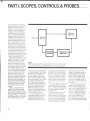
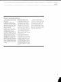
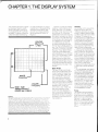
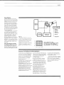


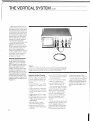


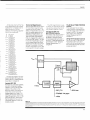


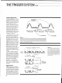


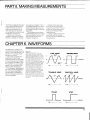
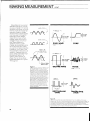
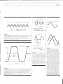

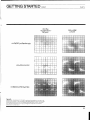

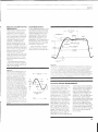
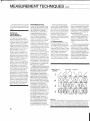


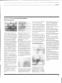

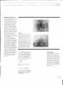

![Manual Audition 4 [By Dr.J.]](http://vs1.manualzilla.com/store/data/005935757_1-4addafd8884e379cc6f9c4cc1fe5fdba-150x150.png)