Download R&S FSW User Manual - Rohde & Schwarz Norway

R&S®FSW
Measurements
Available Measurement Functions
5 Measurements
In the Spectrum application, the R&S FSW provides a variety of different measurement
functions.
●
Basic measurements - measure the spectrum of your signal or watch your signal in
time domain
●
Power measurements - calculate the powers involved in modulated carrier signals
●
Emission measurements - detect unwanted signal emission
●
Statistic measurements - evaluate the spectral distribution of the signal
●
Special measurements - provide characteristic values of the signal
●
EMI measurements - detect electromagnetic interference in the signal
The individual functions are described in detail in the following chapters.
Measurements on I/Q-based data
The I/Q Analyzer application (not Master) in MSRA mode can also perform measurements on the captured I/Q data in the time and frequency domain.
The measurements are configured using the same settings as described here for the
Spectrum application.
The results, however, may differ slightly as hardware settings are not adapted automatically as for the Spectrum application. Additionally, the analysis interval used for the
measurement is indicated as in all MSRA applications.
For more information see the R&S FSW MSRA User Manual.
●
●
●
●
●
●
●
●
●
●
●
●
●
Available Measurement Functions........................................................................101
Channel Power and Adjacent-Channel Power (ACLR) Measurement..................106
Carrier-to-Noise Measurements............................................................................154
Occupied Bandwidth Measurement (OBW)..........................................................158
Spectrum Emission Mask (SEM) Measurement...................................................164
Spurious Emissions Measurement........................................................................195
Statistical Measurements (APD, CCDF)...............................................................208
Time Domain Power Measurement.......................................................................222
Harmonic Distortion Measurement........................................................................227
Third Order Intercept (TOI) Measurement............................................................233
AM Modulation Depth Measurement.....................................................................242
Basic Measurements.............................................................................................245
Electromagnetic Interference (EMI) Measurement (R&S FSW-K54)....................249
5.1 Available Measurement Functions
The measurement function determines which settings, functions and evaluation methods
are available in the R&S FSW. The various measurement functions are described in detail
here. They are selected in the "Select Measurement" dialog box that is displayed when
you press the MEAS key or tap "Select Measurement" in the configuration "Overview".
User Manual 1173.9411.02 ─ 13
101
R&S®FSW
Measurements
Available Measurement Functions
When you select a measurement function, the measurement is started with its default
settings immediately and the corresponding measurement configuration menu is displayed. The measurement configuration menu can be displayed at any time by pressing
the MEAS CONFIG key.
The easiest way to configure measurements is using the configuration "Overview", see ​
chapter 6.1, "Configuration Overview", on page 273.
In addition to the measurement-specific parameters, the general parameters can be configured as usual, see ​chapter 6, "Common Measurement Settings", on page 273. Many
measurement functions provide special result displays or evaluation methods; however,
in most cases the general evaluation methods are also available, see ​chapter 7, "Common Analysis and Display Functions", on page 397.
After a preset, the R&S FSW performs a basic frequency sweep.
Frequency Sweep.......................................................................................................102
Zero Span...................................................................................................................102
Ch Power ACLR..........................................................................................................103
C/N, C/No....................................................................................................................103
OBW............................................................................................................................103
Spectrum Emission Mask............................................................................................104
Spurious Emissions.....................................................................................................104
APD.............................................................................................................................104
CCDF..........................................................................................................................105
Time Domain Power....................................................................................................105
TOI..............................................................................................................................105
AM Mod Depth............................................................................................................105
Harmonic Distortion.....................................................................................................105
EMI..............................................................................................................................106
Marker Functions........................................................................................................106
All Functions Off..........................................................................................................106
Frequency Sweep
A common frequency sweep of the input signal over a specified span. Can be used for
general purposes to obtain basic measurement results such as peak levels and spectrum
traces. The "Frequency" menu is displayed. This is the default measurement if no other
function is selected.
Use the general measurement settings to configure the measurement, e.g. via the
"Overview" (see ​chapter 6, "Common Measurement Settings", on page 273).
Remote command:
​[SENSe:​]FREQuency:​STARt​ on page 765, ​[SENSe:​]FREQuency:​STOP​
on page 765
​INITiate[:​IMMediate]​ on page 635
​INITiate:​CONTinuous​ on page 634
Zero Span
A sweep in the time domain at the specified (center) frequency, i.e. the frequency span
is set to zero. The display shows the time on the x-axis and the signal level on the y-axis,
as on an oscilloscope. On the time axis, the grid lines correspond to 1/10 of the current
sweep time.
User Manual 1173.9411.02 ─ 13
102
R&S®FSW
Measurements
Available Measurement Functions
The "Frequency" menu is displayed. Use the general measurement settings to configure
the measurement, e.g. via the "Overview" (see ​chapter 6, "Common Measurement Settings", on page 273).
Most result evaluations can also be used for zero span measurements, although some
functions (e.g. markers) may work slightly differently and some may not be available. If
so, this will be indicated in the function descriptions (see ​chapter 7, "Common Analysis
and Display Functions", on page 397).
Remote command:
​[SENSe:​]FREQuency:​SPAN​ on page 765
​INITiate[:​IMMediate]​ on page 635
​INITiate:​CONTinuous​ on page 634
Ch Power ACLR
Measures the active channel or adjacent-channel power for one or more carrier signals,
depending on the current measurement configuration, and opens a submenu to configure
the channel power measurement.
For details see ​chapter 5.2, "Channel Power and Adjacent-Channel Power (ACLR) Measurement", on page 106.
Remote command:
CALC:MARK:FUNC:POW:SEL ACP, see ​CALCulate<n>:​MARKer<m>:​FUNCtion:​
POWer:​SELect​ on page 641
Results:
CALC:MARK:FUNC:POW:RES? ACP, see ​CALCulate:​MARKer:​FUNCtion:​POWer:​
RESult?​ on page 639
​chapter 11.5.3, "Measuring the Channel Power and ACLR", on page 643
C/N, C/No
Measures the carrier/noise ratio and opens a submenu to configure the measurement.
Measurements without (C/N) and measurements with reference to the bandwidth (C/No)
are possible.
Carrier/noise measurement is only possible in the frequency domain (span > 0).
For details see ​chapter 5.3, "Carrier-to-Noise Measurements", on page 154.
Remote command:
CALC:MARK:FUNC:POW:SEL CN | CN0​CALCulate<n>:​MARKer<m>:​FUNCtion:​
POWer:​SELect​ on page 641
Results:
CALC:MARK:FUNC:POW:RES? CN | CN0, see ​CALCulate:​MARKer:​FUNCtion:​
POWer:​RESult?​ on page 639
​chapter 11.5.4, "Measuring the Carrier-to-Noise Ratio", on page 670
OBW
Measures the occupied bandwidth, i.e. the bandwidth which must contain a defined percentage of the power, and opens a submenu to configure the measurement. For details
see ​chapter 5.4, "Occupied Bandwidth Measurement (OBW)", on page 158.
User Manual 1173.9411.02 ─ 13
103
R&S®FSW
Measurements
Available Measurement Functions
OBW measurement is only possible in the frequency domain (span > 0).
Remote command:
CALC:MARK:FUNC:POW:SEL OBW​CALCulate<n>:​MARKer<m>:​FUNCtion:​POWer:​
SELect​ on page 641
Results:
CALC:MARK:FUNC:POW:RES? OBW, see ​CALCulate:​MARKer:​FUNCtion:​POWer:​
RESult?​ on page 639
​chapter 11.5.5, "Measuring the Occupied Bandwidth", on page 671
Spectrum Emission Mask
Activates a Spectrum Emission Mask (SEM) measurement, which monitors compliance
with a spectral mask, and opens a submenu to configure the measurement.
For details see ​chapter 5.5, "Spectrum Emission Mask (SEM) Measurement",
on page 164.
Remote command:
SENS:SWE:MODE ESP, see ​[SENSe:​]SWEep:​MODE​ on page 674
Results:
CALC:MARK:FUNC:POW:RES? CPOW | PPOW, see ​CALCulate:​MARKer:​
FUNCtion:​POWer:​RESult?​ on page 639
CALC:LIM:FAIL?, see ​CALCulate:​LIMit<k>:​FAIL​ on page 905
​TRACe<n>[:​DATA]​ on page 853
​TRACe<n>[:​DATA]:​X?​ on page 854
​chapter 11.5.6, "Measuring the Spectrum Emission Mask", on page 673
Spurious Emissions
Activates the Spurious Emissions measurement, which monitors unwanted RF products
outside the assigned frequency band generated by an amplifier. A submenu to configure
the measurement is opened.
For details see ​chapter 5.6, "Spurious Emissions Measurement", on page 195.
Remote command:
SENS:SWE:MODE LIST, see ​[SENSe:​]SWEep:​MODE​ on page 674
Results:
TRAC:DATA? SPUR, see ​TRACe<n>[:​DATA]​ on page 853
​chapter 11.5.7, "Measuring Spurious Emissions", on page 699
APD
Measures the amplitude probability density (APD) and opens a submenu to configure the
measurement.
For details see ​chapter 5.7, "Statistical Measurements (APD, CCDF)", on page 208.
Remote command:
​CALCulate<n>:​STATistics:​APD[:​STATe]​ on page 712
Results:
​CALCulate:​STATistics:​RESult<t>?​ on page 719
User Manual 1173.9411.02 ─ 13
104
R&S®FSW
Measurements
Available Measurement Functions
CCDF
Measures the complementary cumulative distribution function (CCDF) and opens a submenu to configure the measurement.
For details see ​chapter 5.7, "Statistical Measurements (APD, CCDF)", on page 208.
Remote command:
​CALCulate<n>:​STATistics:​CCDF[:​STATe]​ on page 712
Results:
​CALCulate<n>:​STATistics:​CCDF:​X<t>?​ on page 718
​CALCulate:​STATistics:​RESult<t>?​ on page 719
Time Domain Power
Measures the power in zero span and opens a submenu to configure the measurement.
For details see ​chapter 5.12, "Basic Measurements", on page 245.
A time domain power measurement is only possible for zero span.
Remote command:
​CALCulate<n>:​MARKer<m>:​FUNCtion:​SUMMary[:​STATe]​ on page 722
​chapter 11.5.9, "Measuring the Time Domain Power", on page 721
TOI
Measures the third order intercept point and opens a submenu to configure the measurement.
For details see ​chapter 5.10, "Third Order Intercept (TOI) Measurement", on page 233.
Remote command:
​CALCulate<n>:​MARKer<m>:​FUNCtion:​TOI[:​STATe]​ on page 733
​CALCulate<n>:​MARKer<m>:​FUNCtion:​TOI:​RESult?​ on page 733
​chapter 11.5.11, "Measuring the Third Order Intercept Point", on page 732
AM Mod Depth
Measures the AM modulation depth and opens a submenu to configure the measurement. An AM-modulated carrier is required in the window to ensure correct operation.
For details see ​chapter 5.11, "AM Modulation Depth Measurement", on page 242.
Remote command:
​CALCulate<n>:​MARKer<m>:​FUNCtion:​MDEPth[:​STATe]​ on page 735
​CALCulate<n>:​MARKer<m>:​FUNCtion:​MDEPth:​RESult?​ on page 735
​chapter 11.5.12, "Measuring the AM Modulation Depth", on page 734
Harmonic Distortion
Measures the harmonic distortion, including the total harmonic distortion, and opens a
submenu to configure the measurement.
User Manual 1173.9411.02 ─ 13
105
R&S®FSW
Measurements
Channel Power and Adjacent-Channel Power (ACLR) Measurement
For details see ​chapter 5.9, "Harmonic Distortion Measurement", on page 227.
Remote command:
​CALCulate<n>:​MARKer<m>:​FUNCtion:​HARMonics[:​STATe]​ on page 729
First harmonic: ​CALCulate<n>:​MARKer<m>:​FUNCtion:​CENTer​ on page 762.
THD: ​CALCulate<n>:​MARKer<m>:​FUNCtion:​HARMonics:​DISTortion?​
on page 731
List of harmonics: ​CALCulate<n>:​MARKer<m>:​FUNCtion:​HARMonics:​LIST?​
on page 731
​chapter 11.5.10, "Measuring the Harmonic Distortion", on page 729
EMI
Detects electromagnetic interference in the signal, and opens a submenu to configure
the measurement.
For details see ​chapter 5.13, "Electromagnetic Interference (EMI) Measurement
(R&S FSW-K54)", on page 249.
Remote command:
​CALCulate:​MARKer:​FUNCtion:​FMEasurement:​STATe​ on page 737
​chapter 11.5.13, "Remote Commands for EMI Measurements", on page 736
Marker Functions
In addition to the measurement functions, some special marker functions are available.
See ​chapter 7.4.2.3, "Marker Function Configuration", on page 458.
All Functions Off
Switches off all measurement functions and returns to a basic frequency sweep.
5.2 Channel Power and Adjacent-Channel Power (ACLR)
Measurement
Measuring the power in channels adjacent to the carrier or transmission channel is useful
to detect interference. The results are displayed as a bar chart for the individual channels.
●
●
●
●
●
●
●
●
About Channel Power Measurements..................................................................106
Channel Power Results.........................................................................................107
Channel Power Basics..........................................................................................109
Channel Power Configuration...............................................................................119
MSR ACLR Configuration.....................................................................................129
How to Perform Channel Power Measurements...................................................143
Measurement Examples.......................................................................................147
Reference: Predefined CP/ACLR Standards........................................................153
5.2.1 About Channel Power Measurements
Measuring channel power and adjacent channel power is one of the most important tasks
for a signal analyzer with the necessary test routines in the field of digital transmission.
User Manual 1173.9411.02 ─ 13
106
R&S®FSW
Measurements
Channel Power and Adjacent-Channel Power (ACLR) Measurement
While, theoretically, channel power could be measured at highest accuracy with a power
meter, its low selectivity means that it is not suitable for measuring adjacent channel
power as an absolute value or relative to the transmit channel power. The power in the
adjacent channels can only be measured with a selective power meter.
A signal analyzer cannot be classified as a true power meter, because it displays the IF
envelope voltage. However, it is calibrated such as to correctly display the power of a
pure sine wave signal irrespective of the selected detector. This calibration cannot be
applied for non-sinusoidal signals. Assuming that the digitally modulated signal has a
Gaussian amplitude distribution, the signal power within the selected resolution bandwidth can be obtained using correction factors. These correction factors are normally
used by the signal analyzer's internal power measurement routines in order to determine
the signal power from IF envelope measurements. These factors apply if and only if the
assumption of a Gaussian amplitude distribution is correct.
Apart from this common method, the R&S FSW also has a true power detector, i.e. an
RMS detector. It displays the power of the test signal within the selected resolution bandwidth correctly, irrespective of the amplitude distribution, without additional correction
factors being required.
The R&S FSW allows you to perform ACLR measurements on input containing multiple
signals for different communication standards. A measurement standard is provided that
allows you to define multiple discontiguous transmit channels at specified frequencies,
independant from the selected center frequency. The ACLR measurement determines
the power levels of the individual transmit, adjacent, and CACLR channels, as well as
the total power for each subblock of transmit channels.
A detailed measurement example is provided in ​chapter 5.2.7, "Measurement Examples", on page 147.
5.2.2 Channel Power Results
For channel or adjacent-channel power measurements, the individual channels are indicated by different colored bars in the diagram. The height of each bar corresponds to the
measured power of that channel. In addition, the name of the channel ("Adj", "Alt1",
"TX1", etc. or a user-defined name) is indicated above the bar (separated by a line which
has no further meaning). For "Fast ACLR" measurements, which are performed in the
time domain, the power versus time is shown for each channel.
User Manual 1173.9411.02 ─ 13
107
R&S®FSW
Measurements
Channel Power and Adjacent-Channel Power (ACLR) Measurement
Results are provided for the TX channel and the number of defined adjacent channels
above and below the TX channel. If more than one TX channel is defined, the carrier
channel to which the relative adjacent-channel power values should be referenced must
be defined. By default, this is the TX channel with the maximum power.
Table 5-1: Measurements performed depending on the number of adjacent channels
0
Only the channel powers are measured.
1
The channel powers and the power of the upper and lower adjacent channel are measured.
2
The channel powers, the power of the upper and lower adjacent channel, and of the next higher
and lower channel (alternate channel 1) are measured.
3
The channel power, the power of the upper and lower adjacent channel, the power of the next
higher and lower channel (alternate channel 1), and of the next but one higher and lower adjacent
channel (alternate channel 2) are measured.
…
…
12
The channel power, the power of the upper and lower adjacent channel, and the power of all the
higher and lower channels (alternate channels 1 to 11) are measured.
In the R&S FSW's display, only the first neighboring channel of the carrier (TX) channel
is labelled "Adj" (adjacent) channel; all others are labelled "Alt" (alternate) channels. In
this manual, "adjacent" refers to both adjacent and alternate channels.
The measured power values for the TX and adjacent channels are also output as a table
in the second window. Which powers are measured depends on the number of configured
channels.
For each channel, the following values are displayed:
User Manual 1173.9411.02 ─ 13
108
R&S®FSW
Measurements
Channel Power and Adjacent-Channel Power (ACLR) Measurement
Label
Description
Channel
Channel name as specified in the "Channel Settings" (see ​"Channel Names"
on page 129).
Bandwidth
Configured channel bandwidth (see ​"Channel Bandwidths" on page 127)
Offset
Offset of the channel to the TX channel (Configured channel spacing, see ​"Channel
Bandwidths" on page 127)
Power
The measured power values for the TX and lower and upper adjacent channels. The
powers of the transmission channels are output in dBm or dBm/Hz, or in dBc, relative
to the specified reference TX channel.
(Lower/Upper)
Retrieving Results via Remote Control
All or specific channel power measurement results can be retrieved using the
CALC:MARK:FUNC:POW:RES? command from a remote computer (see ​CALCulate:​
MARKer:​FUNCtion:​POWer:​RESult?​ on page 639). Alternatively, the results can be
output as channel power density, i.e. in reference to the measurement bandwidth.
Furthermore, the measured power values of the displayed trace can be retrieved as usual
using the TRAC:DATA? commands (see ​TRACe<n>[:​DATA]​ on page 853). In this case,
the measured power value for each sweep point (by default 1001) is returned.
5.2.3 Channel Power Basics
Some background knowledge on basic terms and principles used in channel power
measurements is provided here for a better understanding of the required configuration
settings.
●
●
●
●
5.2.3.1
Measurement Methods.........................................................................................109
Measurement Repeatability..................................................................................111
Recommended Common Measurement Parameters............................................112
Measurement on Multi-Standard Radio (MSR) Signals........................................116
Measurement Methods
The channel power is defined as the integration of the power across the channel bandwidth.
The Adjacent Channel Leakage Power Ratio (ACLR), also known as the Adjacent
Channel Power Ratio (ACPR), is defined as the ratio between the total power of the
adjacent channel to the carrier channel's power. An ACLR measurement with several
carrier channels (also known as transmission or TX channels) is also possible and is
referred to as a "multicarrier ACLR measurement".
There are two possible methods for measuring channel and adjacent channel power with
a signal analyzer:
●
IBW method (Integration BandWidth method)
●
Fast ACLR (Zero-span method ), i.e. using a channel filter
User Manual 1173.9411.02 ─ 13
109
R&S®FSW
Measurements
Channel Power and Adjacent-Channel Power (ACLR) Measurement
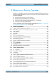
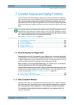
IBW method
When measuring the channel power, the R&S FSW integrates the linear power which
corresponds to the levels of the measurement points within the selected channel. The
signal analyzer uses a resolution bandwidth which is far smaller than the channel bandwidth. When sweeping over the channel, the channel filter is formed by the passband
characteristics of the resolution bandwidth.
Fig. 5-1: Approximating the channel filter by sweeping with a small resolution bandwidth
The following steps are performed:
1. The linear power of all the trace points within the channel is calculated.
Pi = 10(Li/10)
where Pi = power of the trace pixel i
Li = displayed level of trace point i
2. The powers of all trace points within the channel are summed up and the sum is
divided by the number of trace points in the channel.
3. The result is multiplied by the quotient of the selected channel bandwidth and the
noise bandwidth of the resolution filter (RBW).
Since the power calculation is performed by integrating the trace within the channel
bandwidth, this method is called the IBW method (Integration Bandwidth method).
Fast ACLR
The integrated bandwidth method (IBW) calculates channel power and ACLR from the
trace data obtained during a continuous sweep over the selected span. Most parts of this
sweep are neither part of the channel itself nor the defined adjacent channels. Therefore,
most of the samples taken during the sweep time cannot be used for channel power or
ACLR calculation.
To decrease the measurement times, the R&S FSW offers a "Fast ACLR" mode. In Fast
ACLR mode, the power of the frequency range between the channels of interest is not
measured, because it is not required for channel power or ACLR calculation. The measurement time per channel is set with the sweep time. It is equal to the selected measurement time divided by the selected number of channels.
User Manual 1173.9411.02 ─ 13
110
R&S®FSW
Measurements
Channel Power and Adjacent-Channel Power (ACLR) Measurement
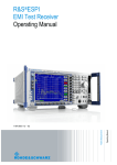
In the "Fast ACLR" mode, the R&S FSW measures the power of each channel in the time
domain, with the defined channel bandwidth, at the center frequency of the channel in
question. The digital implementation of the resolution bandwidths makes it possible to
select filter characteristics that are precisely tailored to the signal. In case of CDMA2000,
for example, the power in the useful channel is measured with a bandwidth of 1.23 MHz
and that of the adjacent channels with a bandwidth of 30 kHz. Therefore the R&S FSW
changes from one channel to the other and measures the power at a bandwidth of
1.23 MHz or 30 kHz using the RMS detector.
Fig. 5-2: Measuring the channel power and adjacent channel power ratio for CDMA2000 signals with
zero span (Fast ACLR)
5.2.3.2
Measurement Repeatability
The repeatability of the results, especially in the narrow adjacent channels, strongly
depends on the measurement time for a given resolution bandwidth. A longer sweep time
may increase the probability that the measured value converges to the true value of the
adjacent channel power, but obviously increases measurement time.
Assuming a measurement with five channels (1 channel plus 2 lower and 2 upper adjacent channels) and a sweep time of 100 ms, a measurement time per channel of 20 ms
is required. The number of effective samples taken into account for power calculation in
one channel is the product of sweep time in channel times the selected resolution bandwidth.
Assuming a sweep time of 100 ms, there are (30 kHz / 4.19 MHz) * 100 ms * 10 kHz ≈
7 samples. Whereas in Fast ACLR mode, there are (100 ms / 5) * 30 kHz ≈ 600 samples.
Comparing these numbers explains the increase of repeatability with a 95% confidence
level (2δ) from ± 2.8 dB to ± 0.34 dB for a sweep time of 100 ms.
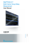
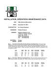
For the same repeatability, the sweep time would have to be set to 8.5 s with the integration method. The ​figure 5-3 shows the standard deviation of the results as a function
of the sweep time.
User Manual 1173.9411.02 ─ 13
111
R&S®FSW
Measurements
Channel Power and Adjacent-Channel Power (ACLR) Measurement
Fig. 5-3: Repeatability of adjacent channel power measurement on CDMA2000 standard signals if the
integration bandwidth method is used
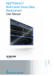
The ​figure 5-4 shows the repeatability of power measurements in the transmit channel
and of relative power measurements in the adjacent channels as a function of sweep
time. The standard deviation of measurement results is calculated from 100 consecutive
measurements. Take scaling into account if comparing power values.
Fig. 5-4: Repeatability of adjacent channel power measurements on CDMA2000 signals in the fast ACLR
mode
5.2.3.3
Recommended Common Measurement Parameters
The following sections provide recommendations on the most important measurement
parameters for channel power measurements.
User Manual 1173.9411.02 ─ 13
112
R&S®FSW
Measurements
Channel Power and Adjacent-Channel Power (ACLR) Measurement
All instrument settings for the selected channel setup (channel bandwidth, channel spacing) can be optimized automatically using the "Adjust Settings" function (see ​"Optimized
Settings (Adjust Settings)" on page 125).
The easiest way to configure a measurement is using the configuration "Overview", see
​chapter 6.1, "Configuration Overview", on page 273.
Sweep Time
The sweep time is selected depending on the desired reproducibility of results. Reproducibility increases with sweep time since power measurement is then performed over a
longer time period. As a general approach, it can be assumed that approx. 500 noncorrelated measured values are required for a reproducibility of 0.5 dB (99 % of the
measurements are within 0.5 dB of the true measured value). This holds true for white
noise. The measured values are considered as non-correlated if their time interval corresponds to the reciprocal of the measured bandwidth.
With IS 136 the measurement bandwidth is approx. 25 kHz, i.e. measured values at an
interval of 40 µs are considered as non-correlated. A measurement time of 40 ms is thus
required per channel for 1000 measured values. This is the default sweep time which the
R&S FSW sets in coupled mode. Approx. 5000 measured values are required for a
reproducibility of 0.1 dB (99 %), i.e. the measurement time is to be increased to 200 ms.
The number of A/D converter values, N, used to calculate the power, is defined by the
sweep time. The time per trace pixel for power measurements is directly proportional to
the selected sweep time.
If the sample detector is used, it is best to select the smallest sweep time possible for a
given span and resolution bandwidth. The minimum time is obtained if the setting is coupled. This means that the time per measurement is minimal. Extending the measurement
time does not have any advantages as the number of samples for calculating the power
is defined by the number of trace points in the channel.
If the RMS detector is used, the repeatability of the measurement results can be influenced by the selection of sweep times. Repeatability is increased at longer sweep times.
If the RMS detector is used, the number of samples can be estimated as follows:
Since only uncorrelated samples contribute to the RMS value, the number of samples
can be calculated from the sweep time and the resolution bandwidth.
Samples can be assumed to be uncorrelated if sampling is performed at intervals of 1/
RBW. The number of uncorrelated samples is calculated as follows:
Ndecorr = SWT * RBW
(Ndecorr means uncorrelated samples)
The number of uncorrelated samples per trace pixel is obtained by dividing Ndecorr by 1001
(= pixels per trace).
The "Sweep Time" can be defined using the softkey in the "Ch Power" menu or in the
"Sweep" configuration dialog box (see ​"Sweep Time" on page 126).
User Manual 1173.9411.02 ─ 13
113
R&S®FSW
Measurements
Channel Power and Adjacent-Channel Power (ACLR) Measurement
Frequency Span
The frequency span must cover at least the channels to be measured plus a measurement margin of approximately 10 %.
If the frequency span is large in comparison to the channel bandwidth (or the adjacentchannel bandwidths) being analyzed, only a few points on the trace are available per
channel. This reduces the accuracy of the waveform calculation for the channel filter
used, which has a negative effect on the measurement accuracy. It is therefore strongly
recommended that the formulas mentioned be taken into consideration when selecting
the frequency span.
The frequency span for the defined channel settings can be optimized using the "Adjust
Settings" function in the "Ch Power" menu or the "General Settings" tab of the "ACLR
Setup" dialog box (see ​"Optimized Settings (Adjust Settings)" on page 125). You can set
the frequency span manually in the "Frequency" configuration dialog box, see ​chapter 6.3.3, "How To Define the Frequency Range", on page 351.
For channel power measurements the "Adjust Settings" function sets the frequency span
as follows:
"(No. of transmission channels – 1) x transmission channel spacing + 2 x transmission
channel bandwidth + measurement margin"
For adjacent-channel power measurements, the "Adjust Settings" function sets the frequency span as a function of the number of transmission channels, the transmission
channel spacing, the adjacent-channel spacing, and the bandwidth of one of adjacentchannels ADJ, ALT1 or ALT2, whichever is furthest away from the transmission channels:
"(No. of transmission channels – 1) x transmission channel spacing + 2 x (adjacentchannel spacing + adjacent-channel bandwidth) + measurement margin"
The measurement margin is approx. 10 % of the value obtained by adding the channel
spacing and the channel bandwidth.
Resolution Bandwidth (RBW)
To ensure both acceptable measurement speed and the required selection (to suppress
spectral components outside the channel to be measured, especially of the adjacent
channels), the resolution bandwidth must not be selected too small or too large. As a
general approach, the resolution bandwidth is to be set to values between 1% and 4%
of the channel bandwidth.
A larger resolution bandwidth can be selected if the spectrum within the channel to be
measured and around it has a flat characteristic. In the standard setting, e.g. for standard
IS95A REV at an adjacent channel bandwidth of 30 kHz, a resolution bandwidth of
30 kHz is used. This yields correct results since the spectrum in the neighborhood of the
adjacent channels normally has a constant level.
The resolution bandwidth for the defined channel settings can be optimized using the
"Adjust Settings" function in the "Ch Power" menu or the "General Settings" tab of the
"ACLR Setup" dialog box (see ​"Optimized Settings (Adjust Settings)" on page 125). You
can set the RBW manually in the "Bandwidth" configuration dialog box, see ​"RBW"
on page 264.
User Manual 1173.9411.02 ─ 13
114
R&S®FSW
Measurements
Channel Power and Adjacent-Channel Power (ACLR) Measurement
With the exception of the IS95 CDMA standards, the "Adjust Settings" function sets the
resolution bandwidth (RBW) as a function of the channel bandwidth:
"RBW ≤ 1/40 of channel bandwidth"
The maximum possible resolution bandwidth (with respect to the requirement RBW ≤
1/40) resulting from the available RBW steps (1, 3) is selected.
Video Bandwidth (VBW)
For a correct power measurement, the video signal must not be limited in bandwidth. A
restricted bandwidth of the logarithmic video signal would cause signal averaging and
thus result in a too low indication of the power (-2.51 dB at very low video bandwidths).
The video bandwidth should therefore be selected at least three times the resolution
bandwidth:
"VBW ≥ 3 x RBW"
The video bandwidth for the defined channel settings can be optimized using the "Adjust
Settings" function in the "Ch Power" menu or the "General Settings" tab of the "ACLR
Setup" dialog box (see ​"Optimized Settings (Adjust Settings)" on page 125). You can set
the VBW manually in the "Bandwidth" configuration dialog box, see ​"VBW"
on page 369.
The video bandwidth (VBW) is set as a function of the channel bandwidth (see formula
above) and the smallest possible VBW with regard to the available step size is selected.
Detector
The RMS detector correctly indicates the power irrespective of the characteristics of the
signal to be measured. The whole IF envelope is used to calculate the power for each
measurement point. The IF envelope is digitized using a sampling frequency which is at
least five times the resolution bandwidth which has been selected. Based on the sample
values, the power is calculated for each measurement point using the following formula:
PRMS 
1 N 2
  si
N i 1
where:
si = linear digitized video voltage at the output of the A/D converter
N = number of A/D converter values per measurement point
PRMS = power represented by a measurement point
When the power has been calculated, the power units are converted into decibels and
the value is displayed as a measurement point.
In principle, the sample detector would be possible as well. Due to the limited number of
measurement points used to calculate the power in the channel, the sample detector
would yield less stable results.
The RMS detector can be set for the defined channel settings automatically using the
"Adjust Settings" function in the "Ch Power" menu or the "General Settings" tab of the
"ACLR Setup" dialog box (see ​"Optimized Settings (Adjust Settings)" on page 125). You
User Manual 1173.9411.02 ─ 13
115
R&S®FSW
Measurements
Channel Power and Adjacent-Channel Power (ACLR) Measurement
can set the detector manually in the "Traces" configuration dialog box, see ​"Detector"
on page 419.
Trace Averaging
Averaging, which is often performed to stabilize the measurement results, leads to a level
indication that is too low and should therefore be avoided. The reduction in the displayed
power depends on the number of averages and the signal characteristics in the channel
to be measured.
The "Adjust Settings" function switches off trace averaging. You can deactivate the trace
averaging manually in the "Traces" configuration dialog box, see ​"Average Mode"
on page 420.
Reference Level
To achieve an optimum dynamic range, the reference level has to be set such that the
signal is as close to the reference level as possible without forcing an overload message
or limiting the dynamic range by an S/N ratio that is too small. Since the measurement
bandwidth for channel power measurements is significantly smaller than the signal bandwidth, the signal path may be overloaded although the trace is still significantly below the
reference level.
The reference level is not influenced by the selection of a predefined standard or by the
automatic setting adjustment. The reference level can be set automatically using the
"Auto Level" function in the AUTO SET menu, or manually in the "Amplitude" menu.
5.2.3.4
Measurement on Multi-Standard Radio (MSR) Signals
Modern base stations may contain multiple signals for different communication standards. A new measurement standard is provided for the R&S FSW ACLR measurement
that allows you to measure such MSR signals, including non-contiguous setups. Multiple
(also non-)contiguous transmit channels can be specified at absolute frequencies, independant from the common center frequency selected for display.
Signal structure
Up to 18 transmit channels can be grouped in a maximum of 5 subblocks. Between two
subblocks, two gaps are defined: a lower gap and an upper gap. Each gap in turn contains
2 channels. The channels in the upper gap are identical to those in the lower gap, but
inverted. To either side of the outermost transmit channels, lower and upper adjacent
channels can be defined as in common ACLR measurement setups.
User Manual 1173.9411.02 ─ 13
116
R&S®FSW
Measurements
Channel Power and Adjacent-Channel Power (ACLR) Measurement
Fig. 5-5: MSR signal structure
Subblock and channel definition
The subblocks are defined by a specified center frequency, RF bandwidth, and number
of transmit channels.
Fig. 5-6: Subblock definition
As opposed to common ACLR channel definitions, the Tx channels are defined at absolute frequencies, rather than by a spacing relative to the (common) center frequency.
Each transmit channel can be assigned a different technology, used to predefine the
required bandwidth.
User Manual 1173.9411.02 ─ 13
117
R&S®FSW
Measurements
Channel Power and Adjacent-Channel Power (ACLR) Measurement
CACLR channels
If two or more subblocks are defined, the power in the gaps between the subblocks must
also be measured (referred to as the Cumulative Adjacent Channel Leakage Ratio
(CACLR) power). According to the MSR standard, the CACLR is measured in the two
channels for the upper and lower gap (thus referred to as CACLR channels). The power
in the CACLR channels is then set in relation to the power of the two closest transmission
channels to either side of the gap.
CACLR channels are defined using bandwidths and spacings, relative to the outer edges
of the surrounding subblocks. Since the upper and lower CACLR channels are identical,
only two channels must be configured. The required spacing can be determined according to the following formula (indicated for lower channels):
Spacing = [CF of the gap channel] - [left subblock center] + ([RF bandwidth of left subblock] /2)
Adjacent channels
Adjacent channels are defined as in common ACLR measurements, using bandwidths
and spacings, however, relative to the start and stop frequency of the total block of transmit channels:
●
The spacing of the lower adjacent channels refers to the CF of the first Tx channel in
the first subblock.
●
The spacing of the upper adjacent channels refers to the CF of the last Tx channel
in the last subblock.
Channel display for MSR signals
As in common ACLR measurements, the individual channels are indicated by different
colored bars in the diagram. The height of each bar corresponds to the measured power
of that channel. In addition, the name of the channel is indicated above the bar. Subblocks
are named A,B,C,D,E and are also indicated by a slim blue bar along the frequency axis.
Note that Tx channel names correspond to the specified technology (for LTE including
the bandwidth), followed by a consecutive number. (If the channel is too narrow to display
the channel name, it is replaced by "..." on the screen.) Channel names cannot be defined
manually. The assigned subblock is indicated with the channel name, e.g.
"B:LTE_5M1" for the first Tx channel in subblock B that uses the LTE 5 MHz bandwidth
technology.
Gap channels (CACLR) are indicated by the names of the surrounding subblocks (e.g.
"AB" for the gap between subblocks A and B), followed by the channel name ("Gap1" or
"Gap2") and an "L" (for lower) or a "U" (for upper). Both the lower and upper gap channels
are displayed. However, if the gap between two subblocks is too narrow, the second gap
channel may not be displayed. If the gap is even narrower, no gap channels are displayed.
Adjacent and alternate channels are displayed as in common ACLR measurements.
Channel power results
The Result Summary for MRS signal measurements is similar to to the table for common
signals (see ​chapter 5.2.2, "Channel Power Results", on page 107). However, the Tx
User Manual 1173.9411.02 ─ 13
118
R&S®FSW
Measurements
Channel Power and Adjacent-Channel Power (ACLR) Measurement
channel results are grouped by subblocks, and subblock totals are provided instead of a
total Tx channel power. Instead of the individual channel frequency offsets, the absolute
center frequencies are indicated for the transmit channels. The CACLR results for each
gap channel are appended at the end of the table. The CACLR results are calculated as
the power in the CACLR channel divided by the power sum of the two closest transmission channels to either side of it.
Restrictions and dependencies
As the signal structure in multi-standard radio signals may vary considerably, the channels can be defined very flexibly for the ACLR measurement with the R&S FSW. No
checks or limitations are implemented concerning the channel definitions, apart from the
maximum number of channels to be defined. Thus, you will not be notified if transmit
channels for a specific subblock lie outside the subblock's defined frequency range, or if
transmit and CACLR channels overlap.
5.2.4 Channel Power Configuration
Channel Power (CP) and Adjacent-Channel Power (ACLR) measurements are selected
via the "Channel Power ACLR" button in the "Select Measurement" dialog box. The
measurement is started immediately with the default settings. It can be configured via the
MEAS CONFIG key or in the "ACLR Setup" dialog box, which is displayed when you
select the "CP/ACLR Config" softkey from the "CH Power" menu.
If the "Multi-Standard Radio" standard is selected (see ​"Standard" on page 121), the
"ACLR Setup" dialog box is replaced by the "MSR ACLR Setup" dialog box. See ​chapter 5.2.5, "MSR ACLR Configuration", on page 129 for a description of these settings.
User Manual 1173.9411.02 ─ 13
119
R&S®FSW
Measurements
Channel Power and Adjacent-Channel Power (ACLR) Measurement
The easiest way to configure a measurement is using the configuration "Overview", see
​chapter 6.1, "Configuration Overview", on page 273.
The remote commands required to perform these tasks are described in ​chapter 11.5.3,
"Measuring the Channel Power and ACLR", on page 643.
●
●
5.2.4.1
General CP/ACLR Measurement Settings............................................................120
Channel Setup......................................................................................................126
General CP/ACLR Measurement Settings
General measurement settings are defined in the "ACLR Setup" dialog, in the "General
Settings" tab.
Standard......................................................................................................................121
└ Predefined Standards...................................................................................121
└ User-Defined Standards...............................................................................121
Number of Channels (Tx, ADJ)...................................................................................123
Reference Channel.....................................................................................................123
Noise cancellation.......................................................................................................124
Fast ACLR...................................................................................................................124
Selected Trace............................................................................................................124
Absolute and Relative Values (ACLR Mode)..............................................................124
Channel Power Levels and Density (Power Unit).......................................................125
Power Mode................................................................................................................125
User Manual 1173.9411.02 ─ 13
120
R&S®FSW
Measurements
Channel Power and Adjacent-Channel Power (ACLR) Measurement
Setting a Fixed Reference for Channel Power Measurements (Set CP Reference)
....................................................................................................................................125
Optimized Settings (Adjust Settings)...........................................................................125
Sweep Time................................................................................................................126
Standard
The main measurement settings can be stored as a standard file. When such a standard
is loaded, the required channel and general measurement settings are automatically set
on the R&S FSW. However, the settings can be changed. Predefined standards are
available for standard measurements, but standard files with user-defined configurations
can also be created.
Note: If the "Multi-Standard Radio" standard is selected, the "ACLR Setup" dialog box is
replaced by the "MSR ACLR Setup" dialog box (see ​chapter 5.2.5, "MSR ACLR Configuration", on page 129).
If any other predefined standard (or "NONE") is selected, the "ACLR Setup" dialog box
is restored (see ​chapter 5.2.4, "Channel Power Configuration", on page 119).
Note that changes in the configuration are not stored when the dialog boxes are
exchanged.
Predefined Standards ← Standard
Predefined standards contain the main measurement settings for standard measurements. When such a standard is loaded, the required channel settings are automatically
set on the R&S FSW. However, the settings can be changed.
The predefined standards contain the following settings:
●
●
●
●
●
●
Channel bandwidths
Channel spacings
Detector
Trace Average setting
Resolution Bandwidth (RBW)
Weighting Filter
Predefined standards can be selected via the "CP/ACLR Standard" softkey in the "CH
Power" menu or in the "General Settings" tab of the "CP/ACLR Setup" dialog box.
For details on the available standards see ​chapter 5.2.8, "Reference: Predefined CP/
ACLR Standards", on page 153.
Remote command:
​CALCulate<n>:​MARKer<m>:​FUNCtion:​POWer:​PRESet​ on page 643
User-Defined Standards ← Standard
In addition to the predefined standards you can save your own standards with your specific measurement settings in an xml file so you can use them again at a later time. Userdefined standards are stored on the instrument in the C:\R_S\instr\acp_std directory.
A sample file is provided for an MSR ACLR measurement (MSR_ACLRExample.xml). It
sets up the measurement for the MSR signal generator waveform described in the file
C:\R_S\instr\user\waveform\MSRA_GSM_WCDMA_LET_GSM.wv.
Note that ACLR user standards are not supported for Fast ACLR and multicarrier ACLR
measurements.
User Manual 1173.9411.02 ─ 13
121
R&S®FSW
Measurements
Channel Power and Adjacent-Channel Power (ACLR) Measurement
Note: User standards created on an analyzer of the R&S FSP family are compatible to
the R&S FSW. User standards created on an R&S FSW, however, are not necessarily
compatible to the analyzers of the R&S FSP family and may not work there.
The following parameter definitions are saved in a user-defined standard:
● Number of adjacent channels
● Channel bandwidth of transmission (Tx), adjacent (Adj) and alternate (Alt) channels
● Channel spacings
● Weighting filters
● Resolution bandwidth
● Video bandwidth
● Detector
● ACLR limits and their state
● Sweep time and sweep time coupling
● Trace and power mode
● (MSR only: subblock and gap channel definition)
User-defined standards are managed in the "Manage" dialog box which is displayed when
you select the "Manage User Standards" button in the "General Settings" tab of the "CP/
ACLR Setup" dialog box.
In the "Manage" dialog box you can save the current measurement settings as a userdefined standard, or load a stored measurement configuration. Furthermore, you can
delete an existing configuration file.
User Manual 1173.9411.02 ─ 13
122
R&S®FSW
Measurements
Channel Power and Adjacent-Channel Power (ACLR) Measurement
For details see ​chapter 5.2.6.4, "How to Manage User-Defined Configurations",
on page 146.
Remote command:
To query all available standards:
​CALCulate<n>:​MARKer<m>:​FUNCtion:​POWer:​STANdard:​CATalog?​
on page 644
To load a standard:
​CALCulate<n>:​MARKer<m>:​FUNCtion:​POWer:​PRESet​ on page 643
To save a standard:
​CALCulate<n>:​MARKer<m>:​FUNCtion:​POWer:​STANdard:​SAVE​ on page 644
To delete a standard:
​CALCulate<n>:​MARKer<m>:​FUNCtion:​POWer:​STANdard:​DELete​ on page 644
Number of Channels (Tx, ADJ)
Up to 18 carrier channels and up to 12 adjacent channels can be defined.
Results are provided for the Tx channel and the number of defined adjacent channels
above and below the Tx channel. If more than one Tx channel is defined, the carrier
channel to which the relative adjacent-channel power values should be referenced must
be defined (see ​"Reference Channel" on page 123).
Note: If several carriers (Tx channels) are activated for the measurement, the number of
sweep points is increased to ensure that adjacent-channel powers are measured with
adequate accuracy.
For more information on how the number of channels affects the measured powers, see
​chapter 5.2.2, "Channel Power Results", on page 107.
Remote command:
Number of Tx channels:
​[SENSe:​]POWer:​ACHannel:​TXCHannel:​COUNt​ on page 648
Number of Adjacent channels:
​[SENSe:​]POWer:​ACHannel:​ACPairs​ on page 645
Reference Channel
The measured power values in the adjacent channels can be displayed relative to the
transmission channel. If more than one Tx channel is defined, you must select which one
is to be used as a reference channel.
Tx Channel 1
Transmission channel 1 is used.
(Not available for MSR ACLR)
Min Power Tx Channel The transmission channel with the lowest power is used as a reference channel.
Max Power Tx Channel The transmission channel with the highest power is used as a reference channel
(Default).
Lowest & Highest
Channel
The outer left-hand transmission channel is the reference channel for the lower
adjacent channels, the outer right-hand transmission channel that for the upper
adjacent channels.
Remote command:
​[SENSe:​]POWer:​ACHannel:​REFerence:​TXCHannel:​MANual​ on page 650
​[SENSe:​]POWer:​ACHannel:​REFerence:​TXCHannel:​AUTO​ on page 650
User Manual 1173.9411.02 ─ 13
123
R&S®FSW
Measurements
Channel Power and Adjacent-Channel Power (ACLR) Measurement
Noise cancellation
The results can be corrected by the instrument's inherent noise, which increases the
dynamic range.
In this case, a reference measurement of the instrument's inherent noise is carried out.
The measured noise power is then subtracted from the power in the channel that is being
analyzed (first active trace only).
The inherent noise of the instrument depends on the selected center frequency, resolution bandwidth and level setting. Therefore, the correction function is disabled whenever
one of these parameters is changed. A disable message is displayed on the screen. To
enable the correction function after changing one of these settings, activate it again. A
new reference measurement is carried out.
Noise cancellation is also available in zero span.
Currently, noise cancellation is only available for the following trace detectors (see ​
"Detector" on page 419):
●
●
●
●
RMS
Average
Sample
Positive Peak
Remote command:
​[SENSe:​]POWer:​NCORrection​ on page 776
Fast ACLR
If activated, instead of using the IBW method, the R&S FSW sets the center frequency
to the different channel center frequencies consecutively and measures the power with
the selected measurement time (= sweep time/number of channels).
Remote command:
​[SENSe:​]POWer:​HSPeed​ on page 656
Selected Trace
The CP/ACLR measurement can be performed on any active trace.
Remote command:
​[SENSe:​]POWer:​TRACe​ on page 642
Absolute and Relative Values (ACLR Mode)
The powers of the adjacent channels are output in dBm or dBm/Hz (absolute values), or
in dBc, relative to the specified reference Tx channel.
"Abs"
The absolute power in the adjacent channels is displayed in the unit of
the y-axis, e.g. in dBm, dBµV.
"Rel"
The level of the adjacent channels is displayed relative to the level of
the transmission channel in dBc.
Remote command:
​[SENSe:​]POWer:​ACHannel:​MODE​ on page 665
User Manual 1173.9411.02 ─ 13
124
R&S®FSW
Measurements
Channel Power and Adjacent-Channel Power (ACLR) Measurement
Channel Power Levels and Density (Power Unit)
By default, the channel power is displayed in absolute values. If "/Hz" is activated, the
channel power density is displayed instead. Thus, the absolute unit of the channel power
is switched from dBm to dBm/Hz.
Note: The channel power density in dBm/Hz corresponds to the power inside a bandwidth
of 1 Hz and is calculated as follows:
"channel power density = channel power – log10(channel bandwidth)"
Thus you can measure the signal/noise power density, for example, or use the additional
functions ​Absolute and Relative Values (ACLR Mode) and ​Reference Channel to obtain
the signal to noise ratio.
Remote command:
​CALCulate<n>:​MARKer<m>:​FUNCtion:​POWer:​RESult:​PHZ​ on page 665
Power Mode
The measured power values can be displayed directly for each trace ("Clear/Write"), or
only the maximum values over a series of measurements can be displayed ("Max
Hold"). In the latter case, the power values are calculated from the current trace and
compared with the previous power value using a maximum algorithm. The higher value
is retained. If "Max Hold" mode is activated, "Pwr Max" is indicated in the table header.
Note that the trace mode remains unaffected by this setting.
Remote command:
​CALCulate<n>:​MARKer<m>:​FUNCtion:​POWer:​MODE​ on page 639
Setting a Fixed Reference for Channel Power Measurements (Set CP Reference)
For pure channel power measurements (no adjacent channels defined) with only one Tx
channel, the currently measured channel power can be used as a fixed reference value
for subsequent channel power measurements.
When you select this button, the channel power currently measured on the Tx channel
is stored as a fixed reference power. In the following channel power measurements, the
power is indicated relative to the fixed reference power. The reference value is displayed
in the "Reference" field (in relative ACLR mode); the default value is 0 dBm.
Note: In adjacent-channel power measurement, the power is always referenced to a
transmission channel (see ​"Reference Channel" on page 123), thus, this function is not
available.
Remote command:
​[SENSe:​]POWer:​ACHannel:​REFerence:​AUTO ONCE​ on page 650
Optimized Settings (Adjust Settings)
All instrument settings for the selected channel setup (channel bandwidth, channel spacing) can be optimized automatically.
The adjustment is carried out only once. If necessary, the instrument settings can be
changed later.
The following settings are optimized by "Adjust Settings":
●
●
●
​"Frequency Span" on page 114
​"Resolution Bandwidth (RBW)" on page 114
​"Video Bandwidth (VBW)" on page 115
User Manual 1173.9411.02 ─ 13
125
R&S®FSW
Measurements
Channel Power and Adjacent-Channel Power (ACLR) Measurement
●
●
​"Detector" on page 115
​"Trace Averaging" on page 116
Note: The reference level is not affected by this function. To adjust the reference level
automatically, use the ​Setting the Reference Level Automatically (Auto Level) function in
the AUTO SET menu.
Remote command:
​[SENSe:​]POWer:​ACHannel:​PRESet​ on page 642
Sweep Time
With the RMS detector, a longer sweep time increases the stability of the measurement
results. For recommendations on setting this parameter, see ​"Sweep Time"
on page 113.
The sweep time can be set via the softkey in the "Ch Power" menu and is identical to the
general setting in the "Sweep" configuration dialog box.
Remote command:
​[SENSe:​]SWEep:​TIME​ on page 772
5.2.4.2
Channel Setup
The "Channel Settings" tab in the "ACLR Setup" dialog box provides all the channel settings to configure the channel power or ACLR measurement. You can define the channel
settings for all channels, independant of the defined number of used Tx or adjacent
channels (see ​"Number of Channels (Tx, ADJ)" on page 123).
For details on setting up channels, see ​chapter 5.2.6.2, "How to Set up the Channels",
on page 144.
In addition to the specific channel settings, the general settings ​"Standard"
on page 121 and ​"Number of Channels (Tx, ADJ)" on page 123 are also available in this
tab.
The following settings are available in individual subtabs of the "Channel Settings" tab.
Channel Bandwidths...................................................................................................127
Channel Spacings.......................................................................................................127
Limit Checking.............................................................................................................128
Weighting Filters.........................................................................................................129
Channel Names..........................................................................................................129
User Manual 1173.9411.02 ─ 13
126
R&S®FSW
Measurements
Channel Power and Adjacent-Channel Power (ACLR) Measurement
Channel Bandwidths
The Tx channel bandwidth is normally defined by the transmission standard. The correct
bandwidth is set automatically for the selected standard. The bandwidth for each channel
is indicated by a colored bar in the display.
For measurements that require channel bandwidths which deviate from those defined in
the selected standard, use the IBW method ("Fast ACLR Off"). With the IBW method, the
channel bandwidth borders are right and left of the channel center frequency. Thus, you
can visually check whether the entire power of the signal under test is within the selected
channel bandwidth.
The value entered for any Tx channel is automatically also defined for all subsequent Tx
channels. Thus, only one value needs to be entered if all Tx channels have the same
bandwidth.
The value entered for any ADJ or ALT channel is automatically also defined for all alternate (ALT) channels. Thus, only one value needs to be entered if all adjacent channels
have the same bandwidth.
Remote command:
​[SENSe:​]POWer:​ACHannel:​BANDwidth|BWIDth[:​CHANnel<ch>]​ on page 646
​[SENSe:​]POWer:​ACHannel:​BANDwidth|BWIDth:​ACHannel​ on page 645
​[SENSe:​]POWer:​ACHannel:​BANDwidth|BWIDth:​ALTernate<ch>​ on page 645
Channel Spacings
Channel spacings are normally defined by the selected standard but can be changed.
If the spacings are not equal, the channel distribution in relation to the center frequency
is as follows:
User Manual 1173.9411.02 ─ 13
127
R&S®FSW
Measurements
Channel Power and Adjacent-Channel Power (ACLR) Measurement
Odd number of Tx channels
The middle Tx channel is centered to center frequency.
Even number of Tx channels
The two Tx channels in the middle are used to calculate the frequency
between those two channels. This frequency is aligned to the center
frequency.
The spacings between all Tx channels can be defined individually. When you change the
spacing for one channel, the value is automatically also defined for all subsequent Tx
channels in order to set up a system with equal Tx channel spacing quickly. For different
spacings, a setup from top to bottom is necessary.
Tx1-2
spacing between the first and the second carrier
Tx2-3
spacing between the second and the third carrier
…
…
If you change the adjacent-channel spacing (ADJ), all higher adjacent channel spacings
(ALT1, ALT2, …) are multiplied by the same factor (new spacing value/old spacing value).
Again, only one value needs to be entered for equal channel spacing. For different spacing, configure the spacings from top to bottom.
For details see ​chapter 5.2.6.2, "How to Set up the Channels", on page 144
Remote command:
​[SENSe:​]POWer:​ACHannel:​SPACing:​CHANnel<ch>​ on page 647
​[SENSe:​]POWer:​ACHannel:​SPACing[:​ACHannel]​ on page 646
​[SENSe:​]POWer:​ACHannel:​SPACing:​ALTernate<ch>​ on page 647
Limit Checking
During an ACLR measurement, the power values can be checked whether they exceed
user-defined or standard-defined limits. A relative or absolute limit can be defined, or
both. Both limit types are considered, regardless whether the measured levels are absolute or relative values. The check of both limit values can be activated independently. If
any active limit value is exceeded, the measured value is displayed in red and marked
by a preceding asterisk in the result table.
User Manual 1173.9411.02 ─ 13
128
R&S®FSW
Measurements
Channel Power and Adjacent-Channel Power (ACLR) Measurement
The results of the power limit checks are also indicated in the STAT:QUES:ACPL status
registry (see ​"STATus:QUEStionable:ACPLimit Register" on page 578).
Remote command:
​CALCulate:​LIMit:​ACPower[:​STATe]​ on page 655
​CALCulate:​LIMit:​ACPower:​ACHannel:​ABSolute:​STATe​ on page 652
​CALCulate:​LIMit:​ACPower:​ACHannel:​ABSolute​ on page 651
​CALCulate:​LIMit:​ACPower:​ACHannel[:​RELative]:​STATe​ on page 653
​CALCulate:​LIMit:​ACPower:​ACHannel[:​RELative]​ on page 652
​CALCulate:​LIMit:​ACPower:​ALTernate<ch>:​ABSolute:​STATe​ on page 653
​CALCulate:​LIMit:​ACPower:​ALTernate<ch>:​ABSolute​ on page 653
​CALCulate:​LIMit:​ACPower:​ALTernate<ch>[:​RELative]:​STATe​ on page 654
​CALCulate:​LIMit:​ACPower:​ALTernate<ch>[:​RELative]​ on page 654
​CALCulate:​LIMit:​ACPower:​ACHannel:​RESult?​ on page 652
Weighting Filters
Weighting filters allow you to determine the influence of individual channels on the total
measurement result. For each channel you can activate or deactivate the use of the
weighting filter and define an individual weighting factor ("Alpha" value).
Weighting filters are not available for all supported standards and cannot always be
defined manually where they are available.
Remote command:
Activating/Deactivating:
​[SENSe:​]POWer:​ACHannel:​FILTer[:​STATe]:​CHANnel<ch>​ on page 650
​[SENSe:​]POWer:​ACHannel:​FILTer[:​STATe]:​ACHannel​ on page 649
​[SENSe:​]POWer:​ACHannel:​FILTer[:​STATe]:​ALTernate<ch>​ on page 649
Alpha value:
​[SENSe:​]POWer:​ACHannel:​FILTer:​ALPHa:​CHANnel<ch>​ on page 649
​[SENSe:​]POWer:​ACHannel:​FILTer:​ALPHa:​ACHannel​ on page 648
​[SENSe:​]POWer:​ACHannel:​FILTer:​ALPHa:​ALTernate<ch>​ on page 648
Channel Names
In the R&S FSW's display, carrier channels are labelled "Tx" by default; the first neighboring channel is labelled "Adj" (adjacent) channel; all others are labelled "Alt" (alternate)
channels. You can define user-specific channel names for each channel which are displayed in the result diagram and result table.
Remote command:
​[SENSe:​]POWer:​ACHannel:​NAME:​ACHannel​ on page 646
​[SENSe:​]POWer:​ACHannel:​NAME:​ALTernate<ch>​ on page 646
​[SENSe:​]POWer:​ACHannel:​NAME:​CHANnel<ch>​ on page 646
5.2.5 MSR ACLR Configuration
ACLR measurements can also be performed on input containing multiple signals for different communication standards. A new measurement standard is provided that allows
you to define multiple discontiguous transmit channels at specified frequencies, independant from the selected center frequency. If the "Multi-Standard Radio" standard is
User Manual 1173.9411.02 ─ 13
129
R&S®FSW
Measurements
Channel Power and Adjacent-Channel Power (ACLR) Measurement
selected (see ​"Standard" on page 121), the "ACLR Setup" dialog box is replaced by the
"MSR ACLR Setup" dialog box.
To display the "MSR ACLR Setup" dialog box dialog box, do one of the following:
●
Select the "CP/ACLR Standard" softkey from the "CH Power" menu and select the
"Multi-Standard Radio" standard. Then select the "CP/ACLR Config" softkey.
●
Select the "CP/ACLR Config" softkey from the "CH Power" menu. Then select the
"Multi-Standard Radio" standard from the "Standard" selection list.
For more information see ​chapter 5.2.3.4, "Measurement on Multi-Standard Radio (MSR)
Signals", on page 116.
The remote commands required to perform these tasks are described in ​chapter 11.5.3,
"Measuring the Channel Power and ACLR", on page 643.
●
●
●
5.2.5.1
General MSR ACLR Measurement Settings.........................................................130
MSR Subblock and Tx Channel Definition............................................................135
MSR Adjacent and Gap Channel Setup................................................................138
General MSR ACLR Measurement Settings
General MSR ACLR measurement settings are defined in the "MSR ACLR Setup" dialog,
in the "MSR General Settings" tab.
Standard......................................................................................................................131
└ Predefined Standards...................................................................................131
└ User-Defined Standards...............................................................................131
Number of Subblocks..................................................................................................133
Reference Channel.....................................................................................................133
Noise cancellation.......................................................................................................133
Selected Trace............................................................................................................134
Absolute and Relative Values (ACLR Mode)..............................................................134
Channel Power Levels and Density (Power Unit).......................................................134
Power Mode................................................................................................................135
Optimized Settings (Adjust Settings)...........................................................................135
User Manual 1173.9411.02 ─ 13
130
R&S®FSW
Measurements
Channel Power and Adjacent-Channel Power (ACLR) Measurement
Standard
The main measurement settings can be stored as a standard file. When such a standard
is loaded, the required channel and general measurement settings are automatically set
on the R&S FSW. However, the settings can be changed. Predefined standards are
available for standard measurements, but standard files with user-defined configurations
can also be created.
Note: If the "Multi-Standard Radio" standard is selected, the "ACLR Setup" dialog box is
replaced by the "MSR ACLR Setup" dialog box (see ​chapter 5.2.5, "MSR ACLR Configuration", on page 129).
If any other predefined standard (or "NONE") is selected, the "ACLR Setup" dialog box
is restored (see ​chapter 5.2.4, "Channel Power Configuration", on page 119).
Note that changes in the configuration are not stored when the dialog boxes are
exchanged.
Predefined Standards ← Standard
Predefined standards contain the main measurement settings for standard measurements. When such a standard is loaded, the required channel settings are automatically
set on the R&S FSW. However, the settings can be changed.
The predefined standards contain the following settings:
●
●
●
●
●
●
Channel bandwidths
Channel spacings
Detector
Trace Average setting
Resolution Bandwidth (RBW)
Weighting Filter
Predefined standards can be selected via the "CP/ACLR Standard" softkey in the "CH
Power" menu or in the "General Settings" tab of the "CP/ACLR Setup" dialog box.
For details on the available standards see ​chapter 5.2.8, "Reference: Predefined CP/
ACLR Standards", on page 153.
Remote command:
​CALCulate<n>:​MARKer<m>:​FUNCtion:​POWer:​PRESet​ on page 643
User-Defined Standards ← Standard
In addition to the predefined standards you can save your own standards with your specific measurement settings in an xml file so you can use them again at a later time. Userdefined standards are stored on the instrument in the C:\R_S\instr\acp_std directory.
A sample file is provided for an MSR ACLR measurement (MSR_ACLRExample.xml). It
sets up the measurement for the MSR signal generator waveform described in the file
C:\R_S\instr\user\waveform\MSRA_GSM_WCDMA_LET_GSM.wv.
Note that ACLR user standards are not supported for Fast ACLR and multicarrier ACLR
measurements.
Note: User standards created on an analyzer of the R&S FSP family are compatible to
the R&S FSW. User standards created on an R&S FSW, however, are not necessarily
compatible to the analyzers of the R&S FSP family and may not work there.
User Manual 1173.9411.02 ─ 13
131
R&S®FSW
Measurements
Channel Power and Adjacent-Channel Power (ACLR) Measurement
The following parameter definitions are saved in a user-defined standard:
● Number of adjacent channels
● Channel bandwidth of transmission (Tx), adjacent (Adj) and alternate (Alt) channels
● Channel spacings
● Weighting filters
● Resolution bandwidth
● Video bandwidth
● Detector
● ACLR limits and their state
● Sweep time and sweep time coupling
● Trace and power mode
● (MSR only: subblock and gap channel definition)
User-defined standards are managed in the "Manage" dialog box which is displayed when
you select the "Manage User Standards" button in the "General Settings" tab of the "CP/
ACLR Setup" dialog box.
In the "Manage" dialog box you can save the current measurement settings as a userdefined standard, or load a stored measurement configuration. Furthermore, you can
delete an existing configuration file.
User Manual 1173.9411.02 ─ 13
132
R&S®FSW
Measurements
Channel Power and Adjacent-Channel Power (ACLR) Measurement
For details see ​chapter 5.2.6.4, "How to Manage User-Defined Configurations",
on page 146.
Remote command:
To query all available standards:
​CALCulate<n>:​MARKer<m>:​FUNCtion:​POWer:​STANdard:​CATalog?​
on page 644
To load a standard:
​CALCulate<n>:​MARKer<m>:​FUNCtion:​POWer:​PRESet​ on page 643
To save a standard:
​CALCulate<n>:​MARKer<m>:​FUNCtion:​POWer:​STANdard:​SAVE​ on page 644
To delete a standard:
​CALCulate<n>:​MARKer<m>:​FUNCtion:​POWer:​STANdard:​DELete​ on page 644
Number of Subblocks
Defines the number of subblocks, i.e. groups of transmission channels in an MSR signal.
For more information see ​chapter 5.2.3.4, "Measurement on Multi-Standard Radio (MSR)
Signals", on page 116.
Remote command:
​[SENSe:​]POWer:​ACHannel:​SBCount​ on page 661
Reference Channel
The measured power values in the adjacent channels can be displayed relative to the
transmission channel. If more than one Tx channel is defined, you must select which one
is to be used as a reference channel.
Tx Channel 1
Transmission channel 1 is used.
(Not available for MSR ACLR)
Min Power Tx Channel The transmission channel with the lowest power is used as a reference channel.
Max Power Tx Channel The transmission channel with the highest power is used as a reference channel
(Default).
Lowest & Highest
Channel
The outer left-hand transmission channel is the reference channel for the lower
adjacent channels, the outer right-hand transmission channel that for the upper
adjacent channels.
Remote command:
​[SENSe:​]POWer:​ACHannel:​REFerence:​TXCHannel:​MANual​ on page 650
​[SENSe:​]POWer:​ACHannel:​REFerence:​TXCHannel:​AUTO​ on page 650
Noise cancellation
The results can be corrected by the instrument's inherent noise, which increases the
dynamic range.
In this case, a reference measurement of the instrument's inherent noise is carried out.
The measured noise power is then subtracted from the power in the channel that is being
analyzed (first active trace only).
User Manual 1173.9411.02 ─ 13
133
R&S®FSW
Measurements
Channel Power and Adjacent-Channel Power (ACLR) Measurement
The inherent noise of the instrument depends on the selected center frequency, resolution bandwidth and level setting. Therefore, the correction function is disabled whenever
one of these parameters is changed. A disable message is displayed on the screen. To
enable the correction function after changing one of these settings, activate it again. A
new reference measurement is carried out.
Noise cancellation is also available in zero span.
Currently, noise cancellation is only available for the following trace detectors (see ​
"Detector" on page 419):
●
●
●
●
RMS
Average
Sample
Positive Peak
Remote command:
​[SENSe:​]POWer:​NCORrection​ on page 776
Selected Trace
The CP/ACLR measurement can be performed on any active trace.
Remote command:
​[SENSe:​]POWer:​TRACe​ on page 642
Absolute and Relative Values (ACLR Mode)
The powers of the adjacent channels are output in dBm or dBm/Hz (absolute values), or
in dBc, relative to the specified reference Tx channel.
"Abs"
The absolute power in the adjacent channels is displayed in the unit of
the y-axis, e.g. in dBm, dBµV.
"Rel"
The level of the adjacent channels is displayed relative to the level of
the transmission channel in dBc.
Remote command:
​[SENSe:​]POWer:​ACHannel:​MODE​ on page 665
Channel Power Levels and Density (Power Unit)
By default, the channel power is displayed in absolute values. If "/Hz" is activated, the
channel power density is displayed instead. Thus, the absolute unit of the channel power
is switched from dBm to dBm/Hz.
Note: The channel power density in dBm/Hz corresponds to the power inside a bandwidth
of 1 Hz and is calculated as follows:
"channel power density = channel power – log10(channel bandwidth)"
Thus you can measure the signal/noise power density, for example, or use the additional
functions ​Absolute and Relative Values (ACLR Mode) and ​Reference Channel to obtain
the signal to noise ratio.
Remote command:
​CALCulate<n>:​MARKer<m>:​FUNCtion:​POWer:​RESult:​PHZ​ on page 665
User Manual 1173.9411.02 ─ 13
134
R&S®FSW
Measurements
Channel Power and Adjacent-Channel Power (ACLR) Measurement
Power Mode
The measured power values can be displayed directly for each trace ("Clear/Write"), or
only the maximum values over a series of measurements can be displayed ("Max
Hold"). In the latter case, the power values are calculated from the current trace and
compared with the previous power value using a maximum algorithm. The higher value
is retained. If "Max Hold" mode is activated, "Pwr Max" is indicated in the table header.
Note that the trace mode remains unaffected by this setting.
Remote command:
​CALCulate<n>:​MARKer<m>:​FUNCtion:​POWer:​MODE​ on page 639
Optimized Settings (Adjust Settings)
All instrument settings for the selected channel setup (channel bandwidth, channel spacing) can be optimized automatically.
The adjustment is carried out only once. If necessary, the instrument settings can be
changed later.
The following settings are optimized by "Adjust Settings":
●
●
●
●
●
​"Frequency Span" on page 114
​"Resolution Bandwidth (RBW)" on page 114
​"Video Bandwidth (VBW)" on page 115
​"Detector" on page 115
​"Trace Averaging" on page 116
Note: The reference level is not affected by this function. To adjust the reference level
automatically, use the ​Setting the Reference Level Automatically (Auto Level) function in
the AUTO SET menu.
Remote command:
​[SENSe:​]POWer:​ACHannel:​PRESet​ on page 642
5.2.5.2
MSR Subblock and Tx Channel Definition
The "Tx Channel Settings" tab in the "MSR ACLR Setup" dialog box provides all the
channel settings to configure subblocks and Tx channels in MSR ACLR measurements.
User Manual 1173.9411.02 ─ 13
135
R&S®FSW
Measurements
Channel Power and Adjacent-Channel Power (ACLR) Measurement
For details on MSR signals see ​chapter 5.2.3.4, "Measurement on Multi-Standard Radio
(MSR) Signals", on page 116.
For details on setting up channels, see ​chapter 5.2.6.3, "How to Configure an MSR ACLR
Measurement", on page 145.
The Tx channel settings for the individual subblocks are configured in individual subtabs
of the "Tx Channel Settings" tab.
Subblock Definition.....................................................................................................136
└ Subblock Center Frequency.........................................................................137
└ RF Bandwidth...............................................................................................137
└ Number of Tx Channels (Tx Count)..............................................................137
Tx Channel Definition..................................................................................................137
└ Tx Center Frequency....................................................................................137
└ Technology Used for Transmission..............................................................138
└ Tx Channel Bandwidth..................................................................................138
└ Weighting Filters...........................................................................................138
Subblock Definition
Subblocks are groups of transmit channels in an MSR signal. Up to 5 subblocks can be
defined. They are defined as an RF bandwidth around a center frequency with a specific
number of transmit channels (max. 18).
Subblocks are named A,B,C,D,E and are indicated by a slim blue bar along the frequency
axis.
User Manual 1173.9411.02 ─ 13
136
R&S®FSW
Measurements
Channel Power and Adjacent-Channel Power (ACLR) Measurement
Subblock Center Frequency ← Subblock Definition
Defines the center of an MSR subblock. Note that the position of the subblock also affects
the position of the adjacent gap channels (CACLR).
Remote command:
​[SENSe:​]POWer:​ACHannel:​SBLock<sb>:​FREQuency:​CENTer​ on page 662
RF Bandwidth ← Subblock Definition
Defines the bandwidth of the individual MSR subblock. Note that subblock ranges also
affect the position of the adjacent gap channels (CACLR).
Remote command:
​[SENSe:​]POWer:​ACHannel:​SBLock<sb>:​RFBWidth​ on page 662
Number of Tx Channels (Tx Count) ← Subblock Definition
Defines the number of transmit channels the specific subblock contains. The maximum
is 18 Tx channels.
Remote command:
​[SENSe:​]POWer:​ACHannel:​SBLock<sb>:​TXCHannel:​COUNt​ on page 663
Tx Channel Definition
As opposed to common ACLR channel definitions, the Tx channels are defined at absolute frequencies, rather than by a spacing relative to the (common) center frequency.
Each transmit channel can be assigned a different technology, used to predefine the
required bandwidth.
The Tx channel settings for the individual subblocks are configured in individual subtabs
of the "Tx Channel Settings" tab.
For details on configuring MSR Tx channels see ​chapter 5.2.6.3, "How to Configure an
MSR ACLR Measurement", on page 145.
Note: Channel names. In MSR ACLR measurements, Tx channel names correspond to
the specified technology (for LTE including the bandwidth), followed by a consecutive
number. (If the channel is too narrow to display the channel name, it is replaced by "..."
on the screen.) Channel names cannot be defined manually. The assigned subblock
(A,B,C,D,E) is indicated with the channel name (e.g. B:LTE_5M1).
Remote command:
​[SENSe:​]POWer:​ACHannel:​SBLock<sb>:​NAME[:​CHANnel<ch>]?​ on page 662
Tx Center Frequency ← Tx Channel Definition
Defines the (absolute) center frequency of an MSR Tx channel. Each Tx channel is
defined independantly of the others; automatic spacing as in common ACLR measurements is not performed.
Note that the position of the first Tx channel in the first subblock and the last Tx channel
in the last subblock also affect the position of the adjacent channels.
Remote command:
​[SENSe:​]POWer:​ACHannel:​SBLock<sb>:​CENTer[:​CHANnel<ch>]​ on page 661
User Manual 1173.9411.02 ─ 13
137
R&S®FSW
Measurements
Channel Power and Adjacent-Channel Power (ACLR) Measurement
Technology Used for Transmission ← Tx Channel Definition
The technology used for transmission by the individual channel can be defined for each
channel. The required channel bandwidth and use of a weighting filter are preconfigured
automatically according to the selected technology standard.
"GSM"
Transmission according to GSM standard
"W-CDMA"
Transmission according to W-CDMA standard
"LTE_1_40""LTE_3_00""LTE_5_00""LTE_10_00""LTE_15_00""LTE_20_00"
Transmission according to LTE standard for different channel bandwidths
"USER"
User-defined transmission; no automatic preconfiguration possible
Remote command:
​[SENSe:​]POWer:​ACHannel:​SBLock<sb>:​TECHnology[:​CHANnel<ch>]​
on page 663
Tx Channel Bandwidth ← Tx Channel Definition
The Tx channel bandwidth is normally defined by the transmission technology standard.
The correct bandwidth is predefined automatically for the selected technology. Each Tx
channel is defined independantly of the others; automatic bandwidth configuration for
subsequent channels as in common ACLR measurements is not performed.
The bandwidth for each channel is indicated by a colored bar in the display.
Remote command:
​[SENSe:​]POWer:​ACHannel:​SBLock<sb>:​BANDwidth|BWIDth[:​CHANnel<ch>]​
on page 661
Weighting Filters ← Tx Channel Definition
Weighting filters allow you to determine the influence of individual channels on the total
measurement result. For each channel you can activate or deactivate the use of the
weighting filter and define an individual weighting factor ("Alpha" value).
Remote command:
Activating/Deactivating:
​[SENSe:​]POWer:​ACHannel:​FILTer:​STATe:​SBLock<sb>:​CHANnel<ch>​
on page 660
Alpha value:
​[SENSe:​]POWer:​ACHannel:​FILTer:​ALPHa:​SBLock<sb>:​CHANnel<ch>​
on page 660
5.2.5.3
MSR Adjacent and Gap Channel Setup
The "Adj/Gap Channel Settings" tab in the "MSR ACLR Setup" dialog box provides all
the channel settings to configure adjacent and gap (CACLR) channels in MSR ACLR
measurements.
User Manual 1173.9411.02 ─ 13
138
R&S®FSW
Measurements
Channel Power and Adjacent-Channel Power (ACLR) Measurement
For details on MSR signals see ​chapter 5.2.3.4, "Measurement on Multi-Standard Radio
(MSR) Signals", on page 116.
For details on setting up channels see ​chapter 5.2.6.3, "How to Configure an MSR ACLR
Measurement", on page 145.
Number of Adjacent Channels (ADJ Count)...............................................................139
Limit Checking.............................................................................................................139
Adjacent Channel Definition........................................................................................140
└ Adjacent Channel Spacings..........................................................................140
└ Adjacent Channel Bandwidths......................................................................140
└ Weighting Filters...........................................................................................141
└ Limit Checking..............................................................................................141
Gap (CACLR) Channel Definition...............................................................................142
└ Gap (CACLR) Channel Spacings.................................................................142
└ Gap (CACLR) Channel Bandwidths..............................................................142
└ Weighting Filters...........................................................................................142
└ Limit Checking..............................................................................................143
Number of Adjacent Channels (ADJ Count)
Defines the number of adjacent channels above and below the Tx channel block in an
MSR signal. The carrier channel to which the relative adjacent-channel power values
should be referenced must be defined (see ​"Reference Channel" on page 123).
Remote command:
​[SENSe:​]POWer:​ACHannel:​ACPairs​ on page 645
Limit Checking
Activates or deactivates limit checks globally for all adjacent and gap (CACLR) channels.
In addition, limits must be defined and activated individually for each channel.
User Manual 1173.9411.02 ─ 13
139
R&S®FSW
Measurements
Channel Power and Adjacent-Channel Power (ACLR) Measurement
The results of the power limit checks are also indicated in the STAT:QUES:ACPL status
registry (see ​"STATus:QUEStionable:ACPLimit Register" on page 578).
Remote command:
​CALCulate:​LIMit:​ACPower[:​STATe]​ on page 655
Adjacent Channel Definition
Defines the channels adjacent to the transmission channel block in MSR signals. A maximum of 12 adjacent channels can be defined.
For MSR signals, adjacent channels are defined in relation to the center frequency of the
first and last transmission channel in the entire block, i.e.:
The lower adjacent channels are defined in relation to the CF of the first Tx channel in
the first subblock.
The upper adjacent channels are defined in relation to the CF of the last Tx channel in
the last subblock.
Adjacent channels are named "Adj" and "Alt1" to "Alt11"; the names cannot be changed
manually.
In all other respects, channel definition is identical to common ACLR measurements.
Adjacent Channel Spacings ← Adjacent Channel Definition
Channel spacings are normally predefined by the selected technology but can be
changed.
For MSR signals, adjacent channels are defined in relation to the center frequency of the
first and last transmission channel in the entire block, i.e.:
The spacing of the lower adjacent channels refers to the CF of the first Tx channel in the
first subblock.
The spacing of the upper adjacent channels refers to the CF of the last Tx channel in the
last subblock.
If you change the adjacent-channel spacing (ADJ), all higher adjacent channel spacings
(ALT1, ALT2, …) are multiplied by the same factor (new spacing value/old spacing value).
Again, only one value needs to be entered for equal channel spacing. For different spacing, configure the spacings from top to bottom.
For details see ​chapter 5.2.6.3, "How to Configure an MSR ACLR Measurement",
on page 145
Remote command:
​[SENSe:​]POWer:​ACHannel:​SPACing[:​ACHannel]​ on page 646
​[SENSe:​]POWer:​ACHannel:​SPACing:​ALTernate<ch>​ on page 647
Adjacent Channel Bandwidths ← Adjacent Channel Definition
The adjacent channel bandwidth is normally predefined by the transmission technology
standard. The correct bandwidth is set automatically for the selected technology. The
bandwidth for each channel is indicated by a colored bar in the display.
User Manual 1173.9411.02 ─ 13
140
R&S®FSW
Measurements
Channel Power and Adjacent-Channel Power (ACLR) Measurement
The value entered for any ADJ or ALT channel is automatically also defined for all subsequent alternate (ALT) channels. Thus, only one value needs to be entered if all adjacent
channels have the same bandwidth.
Remote command:
​[SENSe:​]POWer:​ACHannel:​BANDwidth|BWIDth:​ACHannel​ on page 645
​[SENSe:​]POWer:​ACHannel:​BANDwidth|BWIDth:​ALTernate<ch>​ on page 645
Weighting Filters ← Adjacent Channel Definition
Weighting filters allow you to determine the influence of individual channels on the total
measurement result. For each channel you can activate or deactivate the use of the
weighting filter and define an individual weighting factor ("Alpha" value).
Remote command:
Activating/Deactivating:
​[SENSe:​]POWer:​ACHannel:​FILTer[:​STATe]:​ACHannel​ on page 649
​[SENSe:​]POWer:​ACHannel:​FILTer[:​STATe]:​ALTernate<ch>​ on page 649
Alpha value:
​[SENSe:​]POWer:​ACHannel:​FILTer:​ALPHa:​ACHannel​ on page 648
​[SENSe:​]POWer:​ACHannel:​FILTer:​ALPHa:​ALTernate<ch>​ on page 648
Limit Checking ← Adjacent Channel Definition
During an ACLR measurement, the power values can be checked whether they exceed
user-defined or standard-defined limits. A relative or absolute limit can be defined, or
both, for each individual adjacent channel. Both limit types are considered, regardless
whether the measured levels are absolute or relative values. The check of both limit
values can be activated independently. If any active limit value is exceeded, the measured value is displayed in red and marked by a preceding asterisk in the result table.
Note that in addition to activating limit checking for individual channels, limit checking
must also be activated globally for the MSR ACLR measurement (see ​"Limit Checking"
on page 139).
Remote command:
​CALCulate:​LIMit:​ACPower[:​STATe]​ on page 655
​CALCulate:​LIMit:​ACPower:​ACHannel:​ABSolute:​STATe​ on page 652
​CALCulate:​LIMit:​ACPower:​ACHannel:​ABSolute​ on page 651
​CALCulate:​LIMit:​ACPower:​ACHannel[:​RELative]:​STATe​ on page 653
​CALCulate:​LIMit:​ACPower:​ACHannel[:​RELative]​ on page 652
​CALCulate:​LIMit:​ACPower:​ALTernate<ch>:​ABSolute:​STATe​ on page 653
​CALCulate:​LIMit:​ACPower:​ALTernate<ch>:​ABSolute​ on page 653
​CALCulate:​LIMit:​ACPower:​ALTernate<ch>[:​RELative]:​STATe​ on page 654
​CALCulate:​LIMit:​ACPower:​ALTernate<ch>[:​RELative]​ on page 654
​CALCulate:​LIMit:​ACPower:​ACHannel:​RESult?​ on page 652
User Manual 1173.9411.02 ─ 13
141
R&S®FSW
Measurements
Channel Power and Adjacent-Channel Power (ACLR) Measurement
Gap (CACLR) Channel Definition
Between two subblocks in an MSR signal, two gaps are defined: a lower gap and an
upper gap. Each gap in turn contains 2 channels, the CACLR channels. The channels in
the upper gap are identical to those in the lower gap, but inverted. Thus, in the R&S FSW
MSR ACLR measurement, only 2 gap channels are configured.
Gap channels (CACLR) are indicated by the names of the surrounding subblocks (e.g.
"AB" for the gap between subblocks A and B), followed by the channel name ("Gap1" or
"Gap2") and an "L" (for lower) or a "U" (for upper). Both the lower and upper gap channels
are displayed. However, if the gap between two subblocks is too narrow, the second gap
channel may not be displayed. If the gap is even narrower, no gap channels are displayed.
Gap (CACLR) Channel Spacings ← Gap (CACLR) Channel Definition
CACLR channel spacings are normally predefined by the MSR standard but can be
changed.
CACLR channels are defined using bandwidths and spacings, relative to the outer edges
of the surrounding subblocks. Since the upper and lower CACLR channels are identical,
only two channels must be configured. The required spacing can be determined according to the following formula (indicated for lower channels):
Spacing = [CF of the gap channel] - [left subblock center] + ([RF bandwidth of left subblock] /2)
Spacing = [CF of the gap channel] - [left subblock center] + ([RF bandwidth of left subblock] /2)
(See also ​figure 5-5 and ​figure 5-6.)
For details see ​chapter 5.2.6.3, "How to Configure an MSR ACLR Measurement",
on page 145.
Remote command:
​[SENSe:​]POWer:​ACHannel:​SPACing:​GAP<gap>​ on page 664
Gap (CACLR) Channel Bandwidths ← Gap (CACLR) Channel Definition
The gap channel bandwidth is normally predefined by the transmission technology standard. The correct bandwidth is set automatically for the selected technology. The bandwidth for each channel is indicated by a colored bar in the display (if the gap is not too
narrow, see ​"Channel display for MSR signals" on page 118).
Remote command:
​[SENSe:​]POWer:​ACHannel:​BANDwidth|BWIDth:​GAP<gap>​ on page 659
Weighting Filters ← Gap (CACLR) Channel Definition
Weighting filters allow you to determine the influence of individual channels on the total
measurement result. For each channel you can activate or deactivate the use of the
weighting filter and define an individual weighting factor ("Alpha" value).
Remote command:
​[SENSe:​]POWer:​ACHannel:​FILTer:​STATe:​GAP<gap>​ on page 660
​[SENSe:​]POWer:​ACHannel:​FILTer:​ALPHa:​GAP<gap>​ on page 659
User Manual 1173.9411.02 ─ 13
142
R&S®FSW
Measurements
Channel Power and Adjacent-Channel Power (ACLR) Measurement
Limit Checking ← Gap (CACLR) Channel Definition
During an ACLR measurement, the power values can be checked whether they exceed
user-defined or standard-defined limits. A relative or absolute limit can be defined, or
both, for each individual gap channel. Both limit types are considered, regardless whether
the measured levels are absolute or relative values. The check of both limit values can
be activated independently. If any active limit value is exceeded, the measured value is
displayed in red and marked by a preceding asterisk in the result table.
Note that in addition to activating limit checking for individual channels, limit checking
must also be activated globally for the MSR ACLR measurement (see ​"Limit Checking"
on page 139).
Remote command:
​CALCulate:​LIMit:​ACPower[:​STATe]​ on page 655
​CALCulate:​LIMit:​ACPower:​GAP<gap>:​ABSolute:​STATe​ on page 657
​CALCulate:​LIMit:​ACPower:​GAP<gap>:​ABSolute​ on page 657
​CALCulate:​LIMit:​ACPower:​GAP<gap>[:​RELative:​]STATe​ on page 658
​CALCulate:​LIMit:​ACPower:​GAP<gap>[:​RELative]​ on page 658
​CALCulate:​LIMit:​ACPower:​GAP<gap>:​RESult?​ on page 658
5.2.6 How to Perform Channel Power Measurements
The following step-by-step instructions demonstrate the most common tasks when performing channel power measurements.
●
●
●
●
●
5.2.6.1
How to Perform a Standard Channel Power Measurement..................................143
How to Set up the Channels.................................................................................144
How to Configure an MSR ACLR Measurement...................................................145
How to Manage User-Defined Configurations.......................................................146
How to Compare the Tx Channel Power in Successive Measurements...............147
How to Perform a Standard Channel Power Measurement
Performing a channel power or ACLR measurement according to common standards is
a very easy and straightforward task with the R&S FSW.
1. Press the MEAS key or tap "Select Measurement" in the "Overview".
2. Select "Channel Power ACLR".
The measurement is started immediately with the default settings.
3. Select the "CP / ACLR Standard" softkey and select a standard from the list.
The measurement is restarted with the predefined settings for the selected standard.
4. If necessary, edit the settings for your specific measurement as described in ​chapter 5.2.6.2, "How to Set up the Channels", on page 144, or load a user-defined configuration (see ​"To load a user-defined configuration" on page 147).
User Manual 1173.9411.02 ─ 13
143
R&S®FSW
Measurements
Channel Power and Adjacent-Channel Power (ACLR) Measurement
5.2.6.2
How to Set up the Channels
Channel definition is the basis for measuring power levels in certain frequency ranges.
Usually, the power levels in one or more carrier (Tx) channels and possibly the adjacent
channels are of interest. Up to 18 carrier channels and up to 12 adjacent channels can
be defined.
When a measurement standard is selected in the "Ch Power" menu or the "ACLR
Setup" dialog box, all settings including the channel bandwidths and channel spacings
are set according to the selected standard and can be adjusted afterwards.
Channel setup consists of the following settings:
●
The number of transmission (Tx) and adjacent channels
●
The bandwidth of each channel
●
For multicarrier ACLR measurements: which Tx channel is used as a reference
●
The spacing between the individual channels
●
Optionally: the names of the channels displayed in the diagram and result table
●
Optionally: the influence of individual channels on the total measurement result
("Weighting Filter")
●
Optionally: limits for a limit check on the measured power levels
Changes to an existing standard can be stored as a user-defined standard, see ​chapter 5.2.6.4, "How to Manage User-Defined Configurations", on page 146.
► In the "Ch Power" menu, select the "CP / ACLR Config" softkey, then select the
"Channel Settings" tab to configure the channels in the "ACLR Setup" dialog box.
In the "Channel Setup" dialog box you can define the channel settings for all channels,
independant of the defined number of used Tx or adjacent channels.
To define channel spacings
Channel spacings are normally defined by the selected standard but can be changed.
► In the "Channel Settings" tab of the "ACLR Setup" dialog box, select the "Spacing"
subtab.
The value entered for any Tx channel is automatically also defined for all subsequent
Tx channels. Thus, only one value needs to be entered if all Tx channels have the
same spacing.
If the channel spacing for the adjacent or an alternate channel is changed, all higher
alternate channel spacings are multiplied by the same factor (new spacing value/old
spacing value). The lower adjacent-channel spacings remain unchanged. Only one
value needs to be entered for equal channel spacing.
User Manual 1173.9411.02 ─ 13
144
R&S®FSW
Measurements
Channel Power and Adjacent-Channel Power (ACLR) Measurement
Example: Defining channel spacing
In the default setting, the adjacent channels have the following spacing: 20 kHz ("ADJ"),
40 kHz ("ALT1"), 60 kHz ("ALT2"), 80 kHz ("ALT3"), 100 kHz ("ALT4"), …
If the spacing of the first adjacent channel ("ADJ") is set to 40 kHz, the spacing of all other
adjacent channels is multiplied by factor 2 to result in 80 kHz ("ALT1"), 120 kHz ("ALT2"),
160 kHz ("ALT3"), …
If, starting from the default setting, the spacing of the 5th adjacent channel ("ALT4") is
set to 150 kHz, the spacing of all higher adjacent channels is multiplied by factor 1.5 to
result in 180 kHz ("ALT5"), 210 kHz ("ALT6"), 240 kHz ("ALT7"), …
5.2.6.3
How to Configure an MSR ACLR Measurement
Performing an ACLR measurement on MSR signals is supported by a special configuration with the R&S FSW.
1. Press the MEAS key or tap "Select Measurement" in the "Overview".
2. Select "Channel Power ACLR".
The measurement is started immediately with the default settings.
3. Select the "CP / ACLR Standard" softkey and select the "Multi-Standard Radio"
standard from the list.
4. Select the "CP / ACLR Config" softkey to configure general MSR settings, including
the number of subblocks (up to 5).
5. Select the "Tx Channel Settings" tab to configure the subblocks and transmission
channels.
For each subblock:
a) Define the (center frequency) position and bandwidth of the subblock, as well as
the number of transmission channels it contains.
b) For each transmission channel in the subblock, define the center frequency and
select the technology used for transmission. If necessary, edit the bandwidth and
define the use of a weighting filter for the channel.
6. Select the "Adj/Gap Channel Settings" tab to configure the adjacent and gap
(CACLR) channels.
7. Define the number of adjacent channels and the settings for each channel:
●
●
●
●
The spacing, defined as the distance from the center frequency of the first transmission channel in the first subblock. If the distance between each adjacent
channel and the next is identical, you only need to define the spacing for the first
adjacent channel, the others are adapted automatically.
The bandwidth; if it is identical for all adjacent channels, you only need to define
the bandwidth for the first channel, the others are adapted automatically.
If necessary, a weighting filter
Optionally, define and activate relative or absolute limits, or both, against which
the power levels of the channel are to be checked.
User Manual 1173.9411.02 ─ 13
145
R&S®FSW
Measurements
Channel Power and Adjacent-Channel Power (ACLR) Measurement
8. Define the settings for the two (upper or lower) gap (CACLR) channels; since the
upper and lower channels are identical, it is only necessary to configure two channels.
●
●
●
●
The spacing, defined as the distance from the outer edge of the subblock to the
left or right of the gap. The required spacing can be determined as follows:
Spacing = [CF of the gap channel] - [left subblock center] + ([RF bandwidth of left
subblock] /2)
The bandwidth
If necessary, a weighting filter
Optionally, define and activate relative or absolute limits, or both, against which
the power levels of the channel are to be checked.
9. If power limits are defined and activated, activate global limit checking for the measurement on the "Adj/Gap Channel Settings" tab.
10. Optionally, store the settings for the MSR ACLR measurement as a user-defined
standard as described in ​"To store a user-defined configuration" on page 146. Otherwise the configuration will be lost when you select a different measurement standard!
5.2.6.4
How to Manage User-Defined Configurations
You can define measurement configurations independently of a predefinded standard
and save the current ACLR configuration as a "user standard" in an xml file. You can then
load the file and thus the settings again at a later time.
User-defined standards are not supported for "Fast ACLR" and multicarrier ACLR measurements.
Compatibility to R&S FSP
User standards created on an analyzer of the R&S FSP family are compatible to the
R&S FSW. User standards created on an R&S FSW, however, are not necessarily compatible to the analyzers of the R&S FSP family and may not work there.
To store a user-defined configuration
1. In the "Ch Power" menu, select the "CP / ACLR Config" softkey to display the "ACLR
Setup" dialog box.
2. Configure the measurement as required (see also ​chapter 5.2.6.2, "How to Set up
the Channels", on page 144).
3. In the "General Settings" tab, select the "Manage User Standards" button to display
the "Manage" dialog box.
4. Define a file name for the user standard and select its storage location.
By default, the xml file is stored in C:\R_S\Instr\acp_std\. However, you can
define any other storage location.
5. Select "Save".
User Manual 1173.9411.02 ─ 13
146
R&S®FSW
Measurements
Channel Power and Adjacent-Channel Power (ACLR) Measurement
To load a user-defined configuration
1. In the "General Settings" tab of the "ACLR Setup" dialog box, select the "Manage
User Standards" button to display the "Manage" dialog box.
2. Select the user standard file.
3. Select "Load".
The stored settings are automatically set on the R&S FSW and the measurement is
restarted with the new parameters.
5.2.6.5
How to Compare the Tx Channel Power in Successive Measurements
For pure channel power measurements, where no adjacent channels and only one Tx
channel is defined, you can define a fixed reference power and compare subsequent
measurement results to the stored reference power.
1. Configure a measurement with only one Tx channel and no adjacent channels (see
also ​chapter 5.2.6.2, "How to Set up the Channels", on page 144).
2. Select the "Set CP Reference" softkey in the "Ch Power" menu, or the "Set CP Reference" button in the "ACLR Setup" dialog box.
The channel power currently measured on the Tx channel is stored as a fixed reference power. The reference value is displayed in the "Reference" field of the result
table (in relative ACLR mode).
3. Start a new measurement.
The resulting power is indicated relative to the fixed reference power.
4. Repeat this for any number of measurements.
5. To start a new measurement without the fixed reference, temporarily define a second
channel or preset the instrument.
5.2.7 Measurement Examples
The R&S FSW has test routines for simple channel and adjacent channel power measurements. These routines give quick results without any complex or tedious setting procedures.
●
●
●
Measurement Example 1 – ACPR Measurement on an CDMA2000 Signal........148
Measurement Example 2 – Measuring Adjacent Channel Power of a W-CDMA Uplink
Signal....................................................................................................................149
Measurement Example 3 – Measuring the Intrinsic Noise of the R&S FSW with the
Channel Power Function.......................................................................................152
User Manual 1173.9411.02 ─ 13
147
R&S®FSW
Measurements
Channel Power and Adjacent-Channel Power (ACLR) Measurement
5.2.7.1
Measurement Example 1 – ACPR Measurement on an CDMA2000 Signal
Test setup:
Signal
Generator
R&S FSW
Signal generator settings (e.g. R&S SMU):
Frequency:
850 MHz
Level:
0 dBm
Modulation:
CDMA2000
Procedure:
1. Preset the R&S FSW.
2. Set the center frequency to 850 MHz.
3. Set the span to 4 MHz.
4. Set the reference level to +10 dBm.
5. Select the "Channel Power ACLR" measurement function from the "Select Measurement" dialog box.
6. Set the "CDMA2000 1X" standard for adjacent channel power measurement in the
"ACLR Setup" dialog box.
The R&S FSW sets the channel configuration according to the 2000 standard with 2
adjacent channels above and 2 below the transmit channel. The spectrum is displayed in the upper part of the screen, the numeric values of the results and the
channel configuration in the lower part of the screen. The various channels are represented by vertical lines on the graph.
The frequency span, resolution bandwidth, video bandwidth and detector are
selected automatically to give correct results. To obtain stable results – especially in
the adjacent channels (30 kHz bandwidth) which are narrow in comparison with the
transmission channel bandwidth (1.23 MHz) – the RMS detector is used.
7. Set the optimal reference level and RF attenuation for the applied signal level using
the "Auto Level" function in the AUTO SET menu.
8. Activate "Fast ACLR" mode in the "ACLR Setup" dialog box to increase the repeatability of results.
The R&S FSW sets the optimal RF attenuation and the reference level based on the
transmission channel power to obtain the maximum dynamic range. The ​figure 5-7
shows the result of the measurement.
User Manual 1173.9411.02 ─ 13
148
R&S®FSW
Measurements
Channel Power and Adjacent-Channel Power (ACLR) Measurement
Fig. 5-7: Adjacent channel power measurement on a CDMA2000 1x signal
5.2.7.2
Measurement Example 2 – Measuring Adjacent Channel Power of a W-CDMA
Uplink Signal
Test setup:
Signal
Generator
R&S FSW
Signal generator settings (e.g. R&S FSW SMU):
Frequency:
1950 MHz
Level:
4 dBm
Modulation:
3GPP W-CDMA Reverse Link
Procedure:
1. Preset the R&S FSW.
2. Set the center frequency to 1950 MHz.
3. Select the "Channel Power ACLR" measurement function from the "Select Measurement" dialog box.
4. Set the "W-CDMA 3GPP REV" standard for adjacent channel power measurement
in the "ACLR Setup" dialog box.
User Manual 1173.9411.02 ─ 13
149
R&S®FSW
Measurements
Channel Power and Adjacent-Channel Power (ACLR) Measurement
The R&S FSW sets the channel configuration to the W-CDMA standard for mobiles
with two adjacent channels above and below the transmit channel. The frequency
span, the resolution and video bandwidth and the detector are automatically set to
the correct values. The spectrum is displayed in the upper window and the channel
power, the level ratios of the adjacent channel powers and the channel configuration
in the lower window. The individual channels are displayed as bars in the graph.
5. Set the optimal reference level and RF attenuation for the applied signal level using
the "Auto Level" function.
The R&S FSW sets the optimum RF attenuation and the reference level for the power
in the transmission channel to obtain the maximum dynamic range. The following
figure shows the result of the measurement.
Fig. 5-8: Measuring the relative adjacent channel power on a W-CDMA uplink signal
The R&S FSW measures the power of the individual channels with zero span. A root
raised cosine filter with the parameters α = 0.22 and chip rate 3.84 Mcps (= receive
filter for W-CDMA) is used as channel filter.
Optimum Level Setting for ACLR Measurements on W-CDMA Signals
The dynamic range for ACLR measurements is limited by the thermal noise floor, the
phase noise and the intermodulation (spectral regrowth) of the signal analyzer. The power
values produced by the R&S FSW due to these factors accumulate linearly. They depend
on the applied level at the input mixer. The three factors are shown in the figure below
for the adjacent channel (5 MHz carrier offset).
User Manual 1173.9411.02 ─ 13
150
R&S®FSW
Measurements
Channel Power and Adjacent-Channel Power (ACLR) Measurement
Fig. 5-9: Dynamic range for ACLR measurements on W-CDMA uplink signals as a function of the mixer
level
The level of the W-CDMA signal at the input mixer is shown on the horizontal axis, i.e.
the measured signal level minus the selected RF attenuation. The individual components
which contribute to the power in the adjacent channel and the resulting relative level (total
ACPR) in the adjacent channel are displayed on the vertical axis. The optimum mixer
level is -12 dBm. The relative adjacent channel power (ACPR) at an optimum mixer level
is -77 dBc. Since, at a given signal level, the mixer level is set in 1 dB steps with the
1 dB RF attenuator, the optimum range spreads from -10 dBm to -14 dBm.
To set the attenuation parameter manually, the following method is recommended:
► Set the RF attenuation so that the mixer level (= measured channel power – RF
attenuation) is between -10 dBm and -14 dBm.
This method is automated with the "Auto Level" function. Especially in remote control
mode, e.g. in production environments, it is best to correctly set the attenuation parameters prior to the measurement, as the time required for automatic setting can be saved.
To measure the R&S FSW's intrinsic dynamic range for W-CDMA adjacent channel
power measurements, a filter which suppresses the adjacent channel power is required
at the output of the transmitter. A SAW filter with a bandwidth of 4 MHz, for example, can
be used.
User Manual 1173.9411.02 ─ 13
151
R&S®FSW
Measurements
Channel Power and Adjacent-Channel Power (ACLR) Measurement
5.2.7.3
Measurement Example 3 – Measuring the Intrinsic Noise of the R&S FSW with the
Channel Power Function
Noise in any bandwidth can be measured with the channel power measurement functions. Thus the noise power in a communication channel can be determined, for example.
If the noise spectrum within the channel bandwidth is flat, the noise marker can be used
to determine the noise power in the channel by considering the channel bandwidth. If,
however, phase noise and noise that normally increases towards the carrier is dominant
in the channel to be measured, or if there are discrete spurious signals in the channel,
the channel power measurement method must be used to obtain correct measurement
results.
Test setup:
► Leave the RF input of the R&S FSW open-circuited or terminate it with 50 Ω.
Procedure:
1. Preset the R&S FSW.
2. Set the center frequency to 1 GHz and the span to 1 MHz.
3. To obtain maximum sensitivity, set RF attenuation to 0 dB and the reference level to
-40 dBm.
4. Select the "Channel Power ACLR" measurement function from the "Select Measurement" dialog box.
5. In the "ACLR Setup" dialog box, set up a single Tx channel with the channel bandwidth 1.23 MHz.
6. Select the "Adjust Settings" softkey.
The settings for the frequency span, the bandwidth (RBW and VBW) and the detector
are automatically set to the optimum values required for the measurement.
7. Stabilize the measurement result by increasing the sweep time.
Set the sweep time to 1 s.
The trace becomes much smoother because of the RMS detector and the channel
power measurement display is much more stable.
User Manual 1173.9411.02 ─ 13
152
R&S®FSW
Measurements
Channel Power and Adjacent-Channel Power (ACLR) Measurement
Fig. 5-10: Measurement of the R&S FSW's intrinsic noise power in a 1.23 MHz channel bandwidth.
5.2.8 Reference: Predefined CP/ACLR Standards
When using predefined standards for ACLR measurement, the test parameters for the
channel and adjacent-channel measurements are configured automatically.
You can select a predefined standard via the "CP / ACLR Standard" softkey in the "Ch
Power" menu or the selection list in the "General Settings" tab of the "ACLR Setup" dialog
box (see ​"Standard" on page 121).
Table 5-2: Predefined CP / ACLR standards with remote command parameters
Standard
Remote parameter
None
NONE
Multi-Standard Radio
MSR
EUTRA/LTE Square
EUTRa
EUTRA/LTE Square/RRC
REUTra
W-CDMA 3GPP FWD
FW3Gppcdma
W-CDMA 3GPP REV
RW3Gppcdma
CDMA IS95A FWD
F8CDma
CDMA IS95A REV
R8CDma
CDMA IS95C Class 0 FWD
FIS95c0
CDMA IS95C Class 0 REV
RIS95c0
CDMA J-STD008 FWD
F19Cdma
CDMA J-STD008 REV
R19Cdma
User Manual 1173.9411.02 ─ 13
153
R&S®FSW
Measurements
Carrier-to-Noise Measurements
Standard
Remote parameter
CDMA IS95C Class 1 FWD
FIS95c1
CDMA IS95C Class 1 REV
RIS95c1
CDMA2000
S2CDma
TD-SCDMA FWD
FTCDma
TD-SCDMA REV
TRCDma
WLAN 802.11A
AWLAN
WLAN 802.11B
BWLAN
WIMAX
WIMax
WIBRO
WIBRo
GSM
GSM
RFID 14443
RFID14443
TETRA
TETRa
PDC
PDC
PHS
PHS
CDPD
CDPD
APCO-25 P2
PAPCo25
User Standard
USER
Customized Standard
<string>
For the R&S FSW, the channel spacing is defined as the distance between the center
frequency of the adjacent channel and the center frequency of the transmission channel.
The definition of the adjacent-channel spacing in standards IS95C and CDMA 2000 is
different. These standards define the adjacent-channel spacing from the center of the
transmission channel to the closest border of the adjacent channel. This definition is also
used by the R&S FSW for the standards marked with an asterisk *).
5.3 Carrier-to-Noise Measurements
The R&S FSW can easily determine the carrier-to-noise ratio, also normalized to a 1 Hz
bandwidth.
●
●
●
●
About the Measurement........................................................................................155
Carrier-to-Noise Results........................................................................................155
Carrier-to-Noise Configuration..............................................................................156
How to Determine the Carrier-to-Noise Ratio.......................................................158
User Manual 1173.9411.02 ─ 13
154
R&S®FSW
Measurements
Carrier-to-Noise Measurements
5.3.1 About the Measurement
The largest signal in the frequency span is the carrier. It is searched when the C/N or C/
NO function is activated and is marked using a fixed reference marker ("FXD").
To determine the noise power, a channel with a defined bandwidth at the defined center
frequency is analyzed. The power within this channel is integrated to obtain the noise
power level. (If the carrier is within this channel, an extra step is required to determine
the correct noise power level, see below.)
The noise power of the channel is subtracted from the maximum carrier signal level, and
in the case of a C/NO measurement, it is referred to a 1 Hz bandwidth.
For this measurement, the RMS detector is activated.
The carrier-to-noise measurements are only available in the frequency domain (span >0).
Measurement process
Depending on whether the carrier is inside or outside the analyzed channel, the measurement process for the carrier-to-noise ratio varies:
●
The carrier is outside the analyzed channel: In this case, it is sufficient to switch on
the desired measurement function and to set the channel bandwidth. The carrier/
noise ratio is displayed on the screen.
●
The carrier is inside the analyzed channel: In this case, the measurement must be
performed in two steps:
– First, perform the reference measurement by switching on either the C/N or the
C/NO measurement and waiting for the end of the next measurement run. The
fixed reference marker is set to the maximum of the measured carrier signal.
–
Then, switch off the carrier so that only the noise of the test setup is active in the
channel. The carrier-to-noise ratio is displayed after the subsequent measurement has been completed.
Frequency Span
The frequency span should be set to approximately 4 times the channel bandwidth in
order to measure the carrier-to-noise ratio correctly. This setting is defined automatically
by the "Adjust Settings" function.
5.3.2 Carrier-to-Noise Results
As a result of the carrier-to-noise measurement the evaluated bandwidth and the calculated C/N ratio are displayed in the result window. The fixed reference marker is indicated
in the diagram.
User Manual 1173.9411.02 ─ 13
155
R&S®FSW
Measurements
Carrier-to-Noise Measurements
Remote command:
You can also query the determined carrier-to-noise ratio via the remote command
CALC:MARK:FUNC:POW:RES? CN or CALC:MARK:FUNC:POW:RES? CN0, see ​
CALCulate:​MARKer:​FUNCtion:​POWer:​RESult?​ on page 639.
5.3.3 Carrier-to-Noise Configuration
The Carrier-to-noise ratio (C/N) and the Carrier-to-noise ratio in relation to the bandwidth
(C/N0) measurements are selected via the corresponding button in the "Select Measurement" dialog box. The measurement is started immediately with the default settings. It
can be configured via the MEAS CONFIG key or in the "Carrier Noise" configuration
dialog box, which is displayed as a tab in the "Analysis" dialog box or when you select
the "Carrier Noise Config" softkey from the "Carrier Noise" menu.
Carrier-to-noise measurements are not available in zero span mode.
The easiest way to configure a measurement is using the configuration "Overview", see
​chapter 6.1, "Configuration Overview", on page 273.
User Manual 1173.9411.02 ─ 13
156
R&S®FSW
Measurements
Carrier-to-Noise Measurements
The remote commands required to perform these tasks are described in ​chapter 11.5.4,
"Measuring the Carrier-to-Noise Ratio", on page 670.
C/N..............................................................................................................................157
C/No............................................................................................................................157
Channel Bandwidth.....................................................................................................157
Adjust Settings............................................................................................................157
C/N
Switches the measurement of the carrier/noise ratio on or off. If no marker is active,
marker 1 is activated.
The measurement is performed on the trace that marker 1 is assigned to. To shift marker
1 and measure another trace, use the "Marker to Trace" softkey in the "Marker" menu
(see ​"Assigning the Marker to a Trace" on page 261).
Remote command:
​CALCulate<n>:​MARKer<m>:​FUNCtion:​POWer:​SELect​ on page 641
​CALCulate:​MARKer:​FUNCtion:​POWer:​RESult?​ on page 639
​CALCulate<n>:​MARKer<m>:​FUNCtion:​POWer[:​STATe]​ on page 641
C/No
Switches the measurement of the carrier/noise ratio with reference to a 1 Hz bandwidth
on or off. If no marker is active, marker 1 is activated.
The measurement is performed on the trace that marker 1 is assigned to. To shift marker
1 and measure another trace, use the "Marker to Trace" softkey in the "Marker" menu
(see ​"Assigning the Marker to a Trace" on page 261).
Remote command:
​CALCulate<n>:​MARKer<m>:​FUNCtion:​POWer:​SELect​ on page 641
​CALCulate:​MARKer:​FUNCtion:​POWer:​RESult?​ on page 639
​CALCulate<n>:​MARKer<m>:​FUNCtion:​POWer[:​STATe]​ on page 641
Channel Bandwidth
Defines the measurement channel bandwidth.
The default setting is 14 kHz.
Remote command:
​[SENSe:​]POWer:​ACHannel:​BANDwidth|BWIDth[:​CHANnel<ch>]​ on page 646
Adjust Settings
Enables the RMS detector and adjusts the span to the selected channel bandwidth
according to:
"4 x channel bandwidth + measurement margin"
The adjustment is performed once; if necessary, the setting can be changed later on.
Remote command:
​[SENSe:​]POWer:​ACHannel:​PRESet​ on page 642
User Manual 1173.9411.02 ─ 13
157
R&S®FSW
Measurements
Occupied Bandwidth Measurement (OBW)
5.3.4 How to Determine the Carrier-to-Noise Ratio
1. Press the "C/N, C/NO" softkey to configure the carrier-to-noise ratio measurement.
2. To change the channel bandwidth to be analyzed, press the "Channel Bandwidth"
softkey.
3. To optimize the settings for the selected channel configuration, press the "Adjust
Settings" softkey.
4. To activate the measurements without reference to the bandwidth, press the "C/N"
softkey.
To activate the measurements with reference to the bandwidth, press the "C/NO"
softkey .
5. If the carrier signal is located within the analyzed channel bandwidth, switch off the
carrier signal so that only the noise is displayed in the channel and perform a second
measurement.
The carrier-to-noise ratio is displayed after the measurement has been completed.
5.4 Occupied Bandwidth Measurement (OBW)
An important characteristic of a modulated signal is its occupied bandwidth. In a radio
communications system, for instance, the occupied bandwidth must be limited to enable
distortion-free transmission in adjacent channels.
●
●
●
●
●
About the Measurement........................................................................................158
OBW Results.........................................................................................................160
OBW Configuration...............................................................................................161
How to Determine the Occupied Bandwidth.........................................................163
Measurement Example.........................................................................................163
5.4.1 About the Measurement
The occupied bandwidth is defined as the bandwidth containing a defined percentage of
the total transmitted power. A percentage between 10 % and 99.9 % can be set.
Measurement principle
The bandwidth containing 99% of the signal power is to be determined, for example. The
algorithm first calculates the total power of all displayed points of the trace. In the next
step, the points from the right edge of the trace are summed up until 0.5 % of the total
power is reached. Auxiliary marker 1 is positioned at the corresponding frequency. Then
the points from the left edge of the trace are summed up until 0.5 % of the power is
reached. Auxiliary marker 2 is positioned at this point. 99 % of the power is now between
the two markers. The distance between the two frequency markers is the occupied bandwidth which is displayed in the marker field.
User Manual 1173.9411.02 ─ 13
158
R&S®FSW
Measurements
Occupied Bandwidth Measurement (OBW)
OBW within defined search limits - multicarrier OBW measurement in one sweep
The occupied bandwidth of the signal can also be determined within defined search limits
instead of for the entire signal. Thus, only a single sweep is required to determine the
OBW for a multicarrier signal. To do so, search limits are defined for an individual carrier
and the OBW measurement is restricted to the frequency range contained within those
limits. Then the search limits are adapted for the next carrier and the OBW is automatically
re-calculated for the new range.
For step-by-step instructions see ​"How to determine the OBW for a multicarrier signal
using search limits" on page 163.
Prerequisites
To ensure correct power measurement, especially for noise signals, and to obtain the
correct occupied bandwidth, the following prerequisites and settings are necessary:
●
Only the signal to be measured is displayed in the window, or search limits are defined
to include only one (carrier) signal. An additional signal would falsify the measurement.
●
RBW << occupied bandwidth (approx. 1/20 of occupied bandwidth, for voice communication type: 300 Hz or 1 kHz)
●
VBW ≥ 3 x RBW
●
RMS detector
●
Span ≥ 2 to 3 x occupied bandwidth
Some of the measurement specifications (e.g. PDC, RCR STD-27B) require measurement of the occupied bandwidth using a peak detector. The detector setting of the
R&S FSW has to be changed accordingly then.
User Manual 1173.9411.02 ─ 13
159
R&S®FSW
Measurements
Occupied Bandwidth Measurement (OBW)
5.4.2 OBW Results
As a result of the OBW measurement the occupied bandwidth ("Occ BW") is indicated in
the marker results. Furthermore, the marker at the center frequency and the temporary
markers are indicated.
The measurement is performed on the trace with marker 1. In order to evaluate another
trace, marker 1 must be placed on another trace (see ​Assigning the Marker to a Trace).
The OBW calculation is repeated if the ​Search Limits are changed, without performing a
new sweep. Thus, the OBW for a multicarrier signal can be determined using only one
sweep.
Remote command:
The determined occupied bandwidth can also be queried using the remote command
CALC:MARK:FUNC:POW:RES? OBW or CALC:MARK:FUNC:POW:RES? AOBW. While
the OBW parameter returns only the occupied bandwidth, the AOBW parameter also returns
the position and level of the temporary markers T1 and T2 used to calculate the occupied
bandwidth.
CALC:MARK:FUNC:POW:SEL OBW, see ​CALCulate<n>:​MARKer<m>:​FUNCtion:​
POWer:​SELect​ on page 641
​CALCulate<n>:​MARKer<m>:​FUNCtion:​POWer[:​STATe]​ on page 641
CALC:MARK:FUNC:POW:RES? OBW, see ​CALCulate:​MARKer:​FUNCtion:​POWer:​
RESult?​ on page 639
User Manual 1173.9411.02 ─ 13
160
R&S®FSW
Measurements
Occupied Bandwidth Measurement (OBW)
5.4.3 OBW Configuration
OBW measurements are selected via the "OBW" button in the "Select Measurement"
dialog box. The measurement is started immediately with the default settings. It can be
configured via the MEAS CONFIG key or in the "Occupied Bandwidth" dialog box, which
is displayed as a tab in the "Analysis" dialog box or when you select the "OBW Config"
softkey from the "OBW" menu.
This measurement is not available in zero span.
Configuring search limits for OBW measurement
The OBW measurement uses the same search limits as defined for marker search (see
​"Search Limits" on page 452). However, only the left and right limits are considered.
The remote commands required to perform these tasks are described in ​chapter 11.5.5,
"Measuring the Occupied Bandwidth", on page 671.
% Power Bandwidth....................................................................................................161
Channel Bandwidth.....................................................................................................162
Adjust Settings............................................................................................................162
Search Limits (Left / Right)..........................................................................................162
Deactivating All Search Limits.....................................................................................162
% Power Bandwidth
Defines the percentage of total power in the displayed frequency range which defines the
occupied bandwidth. Values from 10% to 99.9% are allowed.
Remote command:
​[SENSe:​]POWer:​BANDwidth|BWIDth​ on page 672
User Manual 1173.9411.02 ─ 13
161
R&S®FSW
Measurements
Occupied Bandwidth Measurement (OBW)
Channel Bandwidth
Defines the channel bandwidth for the transmission channel in single-carrier measurements. This bandwidth is used to optimize the test parameters (for details see ​"Adjust
Settings" on page 162). The default setting is 14 kHz.
For measurements according to a specific transmission standard, define the bandwidth
specified by the standard for the transmission channel.
For multicarrier measurements this setting is irrelevant.
Remote command:
​[SENSe:​]POWer:​ACHannel:​BANDwidth|BWIDth[:​CHANnel<ch>]​ on page 646
Adjust Settings
Optimizes the instrument settings for the measurement of the occupied bandwidth
according to the specified channel bandwidth.
This function is only useful for single carrier measurements.
All instrument settings relevant for power measurement within a specific frequency range
are optimized:
●
●
●
●
Frequency span: 3 × channel bandwidth
RBW ≤ 1/40 of channel bandwidth
VBW ≥ 3 × RBW
Detector: RMS
The reference level is not affected by "Adjust Settings". For an optimum dynamic range
it should be selected such that the signal maximum is close to the reference level (see ​
"Setting the Reference Level Automatically (Auto Level)" on page 357).
The adjustment is carried out only once. If necessary, the instrument settings can be
changed later.
Remote command:
​[SENSe:​]POWer:​ACHannel:​PRESet​ on page 642
Search Limits (Left / Right)
If activated, limit lines are defined and displayed for the search. Only results within the
limited search range are considered.
For details on limit lines for searches see ​"Peak search limits" on page 439.
Remote command:
​CALCulate:​MARKer:​X:​SLIMits[:​STATe]​ on page 862
​CALCulate:​MARKer:​X:​SLIMits:​LEFT​ on page 863
​CALCulate:​MARKer:​X:​SLIMits:​RIGHT​ on page 863
Deactivating All Search Limits
Deactivates the search range limits.
Remote command:
​CALCulate:​MARKer:​X:​SLIMits[:​STATe]​ on page 862
​CALCulate:​THReshold:​STATe​ on page 864
User Manual 1173.9411.02 ─ 13
162
R&S®FSW
Measurements
Occupied Bandwidth Measurement (OBW)
5.4.4 How to Determine the Occupied Bandwidth
How to determine the OBW for a single signal
1. Select the "OBW" measurement function from the "Select Measurement" dialog box.
2. Select the "OBW Config" softkey to display the "Occupied Bandwidth" configuration
dialog box.
3. Define the percentage of power ("% Power Bandwidth") that defines the bandwidth
to be determined.
4. If necessary, change the channel bandwidth for the transmission channel.
5. To optimize the settings for the selected channel configuration, select "Adjust Settings".
6. Start a sweep.
The result is displayed as OBW in the marker results.
How to determine the OBW for a multicarrier signal using search limits
1. Select the "OBW" measurement function from the "Select Measurement" dialog box.
2. Select the "OBW Config" softkey to display the "Occupied Bandwidth" configuration
dialog box.
3. Define the percentage of power ("% Power Bandwidth") that defines the bandwidth
to be determined.
4. Define search limits so the search area contains only the first carrier signal:
a) Enter values for the left or right limits, or both.
b) Enable the use of the required limits.
5. Start a sweep.
The result for the first carrier is displayed as OBW in the marker results.
6. Change the search limits so the search area contains the next carrier signal as
described in step ​step 4.
The OBW is re-calculated and the result for the next carrier is displayed. A new sweep
is not necessary!
7. Continue in this way until all carriers have been measured.
5.4.5 Measurement Example
In the following example, the bandwidth that occupies 99% of the total power of a PDC
signal at 800 MHz, level 0 dBm is measured.
1. Preset the R&S FSW.
User Manual 1173.9411.02 ─ 13
163
R&S®FSW
Measurements
Spectrum Emission Mask (SEM) Measurement
2. Set the center frequency to 800 MHz.
3. Set the reference level to -10 dBm.
4. Select the "OBW" measurement function from the "Select Measurement" dialog box.
5. Set the percentage of power to 99%.
6. Set the channel bandwidth to 21 kHz as specified by the PDC standard.
7. Optimize the settings for the selected channel configuration by selecting "Adjust Settings".
8. Adjust the reference level to the measured total power by selecting the "Auto
Level" softkey in the AUTO SET menu.
9. The PDC standard requires the peak detector for OBW measurement. In the
"Traces" configuration dialog, set the trace detector to "Positive Peak".
10. Start a sweep.
The result is displayed as OBW in the marker results.
5.5 Spectrum Emission Mask (SEM) Measurement
The R&S FSW supports Spectrum Emission Mask (SEM) measurements.
●
●
●
●
●
●
●
About the Measurement........................................................................................164
Typical Applications..............................................................................................165
SEM Results.........................................................................................................165
SEM Basics...........................................................................................................167
SEM Configuration................................................................................................173
How to Perform a Spectrum Emission Mask Measurement..................................185
Reference: SEM File Descriptions........................................................................189
5.5.1 About the Measurement
The Spectrum Emission Mask (SEM) measurement defines a measurement that monitors compliance with a spectral mask. The mask is defined with reference to the input
signal power. The R&S FSW allows for a flexible definition of all parameters in the SEM
measurement. The analyzer performs measurements in predefined frequency ranges
with settings that can be specified individually for each of these ranges.
SEM measurement configurations can be saved to an xml file which can then be exported
to another application or loaded on the R&S FSW again at a later time. Some predefined
XML files are provided that contain ranges and parameters according to the selected
standard.
In order to improve the performance of the R&S FSW for spectrum emission mask measurements, a "Fast SEM" mode is available.
User Manual 1173.9411.02 ─ 13
164
R&S®FSW
Measurements
Spectrum Emission Mask (SEM) Measurement
Monitoring compliance of the spectrum is supported by a special limit check for SEM
measurements.
5.5.2 Typical Applications
Spectrum Emission Mask measurements are typically performed to ensure that modulated signals remain within the valid signal level ranges defined by a particular transmission standard, both in the transmission channel and neighboring channels. Any violations
of the mask may interfere with other transmissions.
The 3GPP TS 34.122 standard, for example, defines a mask for emissions outside the
transmission channel. This mask is defined relative to the input signal power. Three frequency ranges to each side of the transmission channel are defined.
5.5.3 SEM Results
As a result of the Spectrum Emission Mask measurement, the measured signal levels,
the result of the limit check (mask monitoring) and the defined limit lines are displayed in
a diagram (see also ​chapter 5.5.4.2, "Limit Lines in SEM Measurements",
on page 169). Furthermore, the TX channel power "P" is indicated with the used power
class.
Example:
For example, "P<31" is indicated if the lowest power class is defined from infinity to 31
and the power is currently 17 dBm.
In addition to the graphical results of the SEM measurement displayed in the diagram, a
result table is displayed to evaluate the limit check results (see also ​chapter 5.5.4.2, "Limit
Lines in SEM Measurements", on page 169).
User Manual 1173.9411.02 ─ 13
165
R&S®FSW
Measurements
Spectrum Emission Mask (SEM) Measurement
The following information is provided in the result table:
Label
Description
General Information
Standard
Loaded standard settings
Tx Power
Power of the reference range
Tx Bandwidth
Tx bandwidth used by the reference range
RBW
RBW used by the reference range
Range results
Range Low
Frequency range start for the range the peak value belongs to
Range Up
Frequency range end for the range the peak value belongs to
RBW
RBW of the range
Frequency
Frequency
Power Abs
Absolute power level
Power Rel
Power level relative to the TX channel power
ΔLimit
Deviation of the power level from the defined limit
In which detail the data is displayed in the result table can be defined in the "List Evaluation" settings (see ​chapter 5.5.5.6, "List Evaluation", on page 184). By default, one peak
per range is displayed. However, you can change the settings to display only peaks that
exceed a threshold ("Margin").
In addition to listing the peaks in the list evaluation, detected peaks can be indicated by
blue squares in the diagram ("Show Peaks").
Furthermore, you can save the evaluation list to a file which can be exported to another
application for further analysis.
User Manual 1173.9411.02 ─ 13
166
R&S®FSW
Measurements
Spectrum Emission Mask (SEM) Measurement
Retrieving Results via Remote Control
The measurement results of the spectrum emission mask test can be retrieved using the
CALC:LIM:FAIL? command from a remote computer (see ​CALCulate:​LIMit<k>:​
FAIL​ on page 905 for a detailed description).
The power result for the reference range can be queried using
CALC:MARK:FUNC:POW:RES? CPOW, the peak power for the reference range using
CALC:MARK:FUNC:POW:RES? PPOW, see ​CALCulate:​MARKer:​FUNCtion:​POWer:​
RESult?​ on page 639.
The measured power trace can be queried using TRAC:DATA? and TRAC:DATA:X?, see
​TRACe<n>[:​DATA]​ on page 853 and ​TRACe<n>[:​DATA]:​X?​ on page 854:
The measured peak power list can be queried using TRAC:DATA? LIST​TRACe<n>[:​
DATA]​ on page 853.
5.5.4 SEM Basics
Some background knowledge on basic terms and principles used in SEM measurements
is provided here for a better understanding of the required configuration settings.
●
●
●
●
5.5.4.1
Ranges and Range Settings.................................................................................167
Limit Lines in SEM Measurements........................................................................169
Fast SEM Measurements......................................................................................171
Multi-Standard Radio (MSR) SEM Measurements...............................................172
Ranges and Range Settings
In the Spectrum Emission Mask measurements, a range defines a segment for which
you can define the following parameters separately:
●
Start and stop frequency
●
RBW
●
VBW
●
Sweep time
●
Sweep points
●
Reference level
●
Attenuator settings
●
Preamplifier settings
●
Transducer settings
●
Limit values
Via the sweep list, you define the ranges and their settings. For details on settings refer
to ​chapter 5.5.5.1, "Sweep List", on page 173.
For details on defining the limits (masks) see ​chapter 5.5.4.2, "Limit Lines in SEM Measurements", on page 169.
User Manual 1173.9411.02 ─ 13
167
R&S®FSW
Measurements
Spectrum Emission Mask (SEM) Measurement
For details on defining the limits (masks) see the base unit description "Working with
Lines in SEM".
Range definition
After a preset, the sweep list contains a set of default ranges and parameters. For each
range, you can change the parameters listed above. You can insert or delete ranges.
The changes of the sweep list are only kept until you load another parameter set (by
pressing PRESET or by loading an XML file). If you want a parameter set to be available
permanently, create an XML file for this configuration (for details refer to ​"How to save a
user-defined SEM settings file" on page 187).
If you load one of the provided XML files, the sweep list contains ranges and parameters
according to the selected standard.
Reference range
The range centered around the center frequency is defined as the reference range for all
other ranges in the sweep list. All range limits are defined in relation to the reference
range. Power levels in the result table are also calculated in relation to the reference
range. You can define whether the power used for reference is the peak power level or
the integrated power of the reference range. In the "Sweep List", the reference range is
highlighted in blue and cannot be deleted.
Rules
The following rules apply to ranges:
●
The minimum span of a range is 20 Hz.
●
The individual ranges must not overlap (but may have gaps).
●
The maximum number of ranges is 30 (in frimware versions < 1.60: 20 ranges).
●
The minimum number of ranges is 3.
●
The reference range cannot be deleted.
●
The reference range has to be centered on the center frequency.
●
The minimum span of the reference range is given by the current TX Bandwidth.
●
Frequency values for each range have to be defined relative to the center frequency.
In order to change the start frequency of the first range or the stop frequency of the last
range, select the appropriate span with the SPAN key. If you set a span that is smaller
than the overall span of the ranges, the measurement includes only the ranges that lie
within the defined span and have a minimum span of 20 Hz. The first and last ranges are
adapted to the given span as long as the minimum span of 20 Hz is not violated.
Symmetrical ranges
You can easily define a sweep list with symmetrical range settings, i.e. the ranges to the
left and right of the reference range are defined symmectrically. When symmetrical setup
is activated, the current sweep list configuration is changed to define a symmetrical setup
regarding the reference range. The number of ranges to the left of the reference range
is reflected to the right, i.e. any missing ranges on the right are inserted, while superfluous
User Manual 1173.9411.02 ─ 13
168
R&S®FSW
Measurements
Spectrum Emission Mask (SEM) Measurement
ranges are removed. The values in the ranges to the right of the reference range are
adapted symmetrically to those in the left ranges.
Symmetrical ranges fulfull the conditions required for "Fast SEM" mode (see ​chapter 5.5.4.3, "Fast SEM Measurements", on page 171).
Power classes
If the signal power level to be monitored may vary and the limits will vary accordingly,
you can define power classes, which can then be assigned to the frequency ranges. Thus,
the limits for the signal levels can be defined differently for varying input levels. For
instance, for higher input levels a transmission standard may allow for higher power levels
in adjacent channels, whereas for lower input levels the allowed deviation may be stricter.
Up to four different power classes can be defined.
5.5.4.2
Limit Lines in SEM Measurements
On the R&S FSW, the spectrum emission mask is defined using limit lines. Limit lines
allow you to check the measured data against specified limit values. Generally, it is possible to define limit lines for any measurement in the Spectrum application using the
LINES key. For SEM measurements, however, special limit lines are available via the
"Sweep List", and it is strongly recommended that you use only these limit line definitions.
In the "Sweep List" you can define a limit line for each power class that varies its level
according to the specified frequency ranges. Distinguished limit lines
("_SEM_LINE_ABS<0...3>"/ "_SEM_LINE_REL<0...3>") are automatically defined for
each power class according to the current "Sweep List" settings every time the settings
change.
The limit line defined for the currently used power class is indicated by a red line in the
display, and the result of the limit check is indicated at the top of the diagram. Note that
only "Pass" or "Fail" is indicated; a "margin" function as for general limit lines is not available.
User Manual 1173.9411.02 ─ 13
169
R&S®FSW
Measurements
Spectrum Emission Mask (SEM) Measurement
The indicated limit line depends on the settings in the "Sweep List". Several types of limit
checks are possible:
Table 5-3: Limit check types
Limit check type
Pass/fail criteria
Absolute
Absolute power levels may not exceed Defined by the "Abs Limit Start"/ "Abs Limit
limit line
Stop" values for each range
Relative
Power deviations relative to the TX
channel power may not exceed limit
line
Defined by the "Rel Limit Start"/ "Rel Limit
Stop" values (relative to the TX channel power),
fixed for each range.
Relative with function f(x)
If the power exceeds both the absolute and the relative limits, the check
fails.
Defined by the maximum of the absolute or relative (relative to the TX channel power) "Rel
Limit Start"/ "Rel Limit Stop" values for each
range. Thus, the start or stop point of the limit
range, or both, are variable (since the maximum
may vary).
Abs and Rel
If the power exceeds both the absolute and the relative limits, the check
fails.
The less strict (higher) limit line is displayed for
each range.
Abs or Rel
Limit line definition
If you use a function to define the relative limit
start or stop value, the signal is checked against
an additional condition: the power must exceed
the absolute limit, as well as the absolute and
relative function values.
If the power exceeds either the abso- The stricter (lower) limit line is displayed for
lute or the relative limits, the check
each range.
fails.
If you use a function to define the relative limit
start or stop value, the signal is checked against
an additional condition: if the power exceeds
the absolute limit, or the higher of the absolute
and relative function values, the check fails.
Relative limit line functions
A new function allows you to define limit lines whose start or end points (or both) are
variable, depending on the carrier power. Thus, the resulting limit line may change its
slope within the range, depending on the carrier power. Common relative limit lines are
calculated once for the defined start and end points and maintain a constant slope.
If the relative limit value function is used in combination with the "Abs and Rel" or "Abs
or Rel" limit check types, an additional condition is considered for the limit check (see ​
table 5-3).
Limit check results in the evaluation list
The largest deviations of the power from the limit line for each range are displayed in the
evaluation list. Furthermore, the absolute powers for those values, as well as the relative
deviation from the TX channel power are displayed. Values that exceed the limit are
indicated in red and by an asterisk (*).
User Manual 1173.9411.02 ─ 13
170
R&S®FSW
Measurements
Spectrum Emission Mask (SEM) Measurement
Although a margin functionality is not available for the limit check, a margin (threshold)
for the peak values to be displayed in the evaluation list can be defined in the list evaluation settings. For details see ​chapter 5.5.5.6, "List Evaluation", on page 184.
5.5.4.3
Fast SEM Measurements
In order to improve the performance of the R&S FSW for spectrum emission mask measurements, a "Fast SEM" mode is available. If this mode is activated, several consecutive
ranges with identical sweep settings are combined to one sweep internally, which makes
the measurement considerably more efficient. The displayed results remain unchanged
and still consist of several ranges. Thus, measurement settings that apply only to the
results, such as limits or transducer factors, can nevertheless be defined individually for
each range.
Prerequisites
"Fast SEM" mode is available if the following criteria apply:
●
The frequency ranges are consecutive, without frequency gaps
●
The following sweep settings are identical (for details see ​chapter 5.5.5.1, "Sweep
List", on page 173):
– Filter Type
–
RBW
–
VBW
–
Sweep Time Mode
–
Reference Level
–
Rf Attenuation Mode
–
RF Attenuation
–
Preamplificiation
Activating Fast SEM mode
"Fast SEM" mode is activated in the sweep list (see ​chapter 5.5.5.1, "Sweep List",
on page 173) or using a remote command. Activating the mode for one range automatically activates it for all ranges in the sweep list.
Remote command:
​[SENSe:​]ESPectrum:​HighSPeed​ on page 676
Consequences
When the "Fast SEM" mode is activated, the ranges for which these criteria apply are
displayed as one single range. The sweep time is defined as the sum of the individual
sweep times, initially, but can be changed.
User Manual 1173.9411.02 ─ 13
171
R&S®FSW
Measurements
Spectrum Emission Mask (SEM) Measurement
If "Symmetrical Setup" mode is active when "Fast SEM" mode is activated, not all sweep
list settings can be configured symmetrically automatically (see also ​"Symmetric
Setup" on page 177).
Any other changes to the sweep settings of the combined range are applied to each
included range and remain changed even after deactivating "Fast SEM" mode.
Example
Fig. 5-11: Sweep list using Fast SEM mode
In ​figure 5-11, a sweep list is shown for which Fast SEM is activated. The formerly 5
separately defined ranges are combined to 2 sweep ranges internally.
5.5.4.4
Multi-Standard Radio (MSR) SEM Measurements
Multi-standard radio (MSR) measurements allow you to perform SEM tests on signals
with multiple carriers using different digital standards. MSR measurements are described
in the specification 3GPP TS 37.141. Various typical combinations of standards for base
station tests are described, e.g. LTE FDD and W-CDMA carriers. By performing an MSR
SEM measurement you can determine if or how the different carriers affect each other,
i.e. if unwanted emissions occur. On the R&S FSW, the MSR SEM measurement is a
standard measurement as for single carriers. The MSR settings merely provide a convenient way of configuring the sweep list for all required ranges according to the specification very quickly.
User Manual 1173.9411.02 ─ 13
172
R&S®FSW
Measurements
Spectrum Emission Mask (SEM) Measurement
5.5.5 SEM Configuration
SEM measurements are selected via the "Spectrum Emission Mask" button in the "Select
Measurement" dialog box. The measurement is started immediately with the default settings. It can be configured via the MEAS CONFIG key or in the "Spectrum Emission
Mask" configuration dialog box, which is displayed when you select the "SEM Setup"
button in the "Overview" or one of the softkeys from the "SEMask" menu.
The remote commands required to perform these tasks are described in ​chapter 11.5.6,
"Measuring the Spectrum Emission Mask", on page 673.
The following settings are available in individual tabs of the "Spectrum Emission Mask"
configuration dialog box.
●
●
●
●
●
●
5.5.5.1
Sweep List.............................................................................................................173
Reference Range..................................................................................................178
Power Classes......................................................................................................179
MSR Settings........................................................................................................180
Standard Files.......................................................................................................182
List Evaluation.......................................................................................................184
Sweep List
For SEM measurements, the input signal is split into several frequency ranges which are
swept individually and for which different limitations apply. In the "Sweep List" tab of the
"Spectrum Emission Mask" dialog box you configure the individual frequency ranges and
mask limits.
If you edit the sweep list, always follow the rules and consider the limitations described
in ​chapter 5.5.4.1, "Ranges and Range Settings", on page 167.
User Manual 1173.9411.02 ─ 13
173
R&S®FSW
Measurements
Spectrum Emission Mask (SEM) Measurement
Range Start / Range Stop...........................................................................................174
Fast SEM....................................................................................................................174
Filter Type...................................................................................................................174
RBW............................................................................................................................175
VBW............................................................................................................................175
Sweep Time Mode......................................................................................................175
Sweep Time................................................................................................................175
Ref. Level....................................................................................................................175
RF Att. Mode...............................................................................................................175
RF Attenuator..............................................................................................................176
Preamp........................................................................................................................176
Transd. Factor.............................................................................................................176
Limit Check 1-4...........................................................................................................176
Abs Limit Start/Stop....................................................................................................176
Rel Limit Start/Stop.....................................................................................................176
Insert before/after Range............................................................................................177
Delete Range..............................................................................................................177
Symmetric Setup.........................................................................................................177
Range Start / Range Stop
Sets the start frequency/stop frequency of the selected range.
In order to change the start/stop frequency of the first or last range, respectively, select
the appropriate span with the SPAN key. If you set a span that is smaller than the overall
span of the ranges, the measurement includes only the ranges that lie within the defined
span and have a minimum span of 20 Hz. The first and last ranges are adapted to the
given span as long as the minimum span of 20 Hz is not violated.
Frequency values for each range have to be defined relative to the center frequency. The
reference range has to be centered on the center frequency. The minimum span of the
reference range is given by the current ​Channel Power Settings.
Remote command:
​[SENSe:​]ESPectrum:​RANGe<range>[:​FREQuency]:​STARt​ on page 678
​[SENSe:​]ESPectrum:​RANGe<range>[:​FREQuency]:​STOP​ on page 678
Fast SEM
Activates "Fast SEM" mode for all ranges in the sweep list. For details see ​chapter 5.5.4.3,
"Fast SEM Measurements", on page 171.
Note: If "Fast SEM" mode is deactivated while "Symmetrical Setup" mode is on, "Symmetrical Setup" mode is automatically also deactivated.
If "Fast SEM" mode is activated while "Symmetrical Setup" mode is on, not all range
settings can be set automatically.
Remote command:
​[SENSe:​]ESPectrum:​HighSPeed​ on page 676
Filter Type
Sets the filter type for this range.
User Manual 1173.9411.02 ─ 13
174
R&S®FSW
Measurements
Spectrum Emission Mask (SEM) Measurement
For details on filter types see ​chapter 6.5.1.6, "Which Data May Pass: Filter Types",
on page 365.
Remote command:
​[SENSe:​]ESPectrum:​RANGe<range>:​FILTer:​TYPE​ on page 677
RBW
Sets the RBW value for this range.
For details on the RBW see ​chapter 6.5.1.1, "Separating Signals by Selecting an Appropriate Resolution Bandwidth", on page 362.
Remote command:
​[SENSe:​]ESPectrum:​RANGe<range>:​BANDwidth[:​RESolution]​ on page 676
VBW
Sets the VBW value for this range.
For details on the VBW see ​chapter 6.5.1.2, "Smoothing the Trace Using the Video
Bandwidth", on page 363.
Remote command:
​[SENSe:​]ESPectrum:​RANGe<range>:​BANDwidth:​VIDeo​ on page 676
Sweep Time Mode
Activates or deactivates the auto mode for the sweep time.
For details on the sweep time mode see ​chapter 6.5.1.7, "How Long the Data is Measured: Sweep Time", on page 366
Remote command:
​[SENSe:​]ESPectrum:​RANGe<range>:​SWEep:​TIME:​AUTO​ on page 687
Sweep Time
Sets the sweep time value for the range.
For details on the sweep time see ​chapter 6.5.1.7, "How Long the Data is Measured:
Sweep Time", on page 366
Remote command:
​[SENSe:​]ESPectrum:​RANGe<range>:​SWEep:​TIME​ on page 686
Ref. Level
Sets the reference level for the range.
For details on the reference level see ​chapter 6.4.1.1, "Reference Level", on page 353.
Remote command:
​[SENSe:​]ESPectrum:​RANGe<range>:​RLEVel​ on page 686
RF Att. Mode
Activates or deactivates the auto mode for RF attenuation.
For details on attenuation see ​chapter 6.4.1.2, "RF Attenuation", on page 354.
Remote command:
​[SENSe:​]ESPectrum:​RANGe<range>:​INPut:​ATTenuation:​AUTO​ on page 679
User Manual 1173.9411.02 ─ 13
175
R&S®FSW
Measurements
Spectrum Emission Mask (SEM) Measurement
RF Attenuator
Sets the attenuation value for that range.
For details on attenuation see ​chapter 6.4.1.2, "RF Attenuation", on page 354.
Remote command:
​[SENSe:​]ESPectrum:​RANGe<range>:​INPut:​ATTenuation​ on page 679
Preamp
Switches the preamplifier on or off.
For details on the preamplifier see ​"Preamplifier (option B24)" on page 358.
Remote command:
​[SENSe:​]ESPectrum:​RANGe<range>:​INPut:​GAIN:​STATe​ on page 680
Transd. Factor
Sets a transducer for the specified range. You can only choose a transducer that fulfills
the following conditions:
●
●
●
The transducer overlaps or equals the span of the range.
The x-axis is linear.
The unit is dB.
For details on transducers see ​chapter 9.2, "Basics on Transducer Factors",
on page 513.
Remote command:
​[SENSe:​]ESPectrum:​RANGe<range>:​TRANsducer​ on page 687
Limit Check 1-4
Sets the type of limit check for all ranges.
For details on limit checks see ​chapter 5.5.4.2, "Limit Lines in SEM Measurements",
on page 169.
The limit state affects the availability of all limit settings.
Depending on the number of active power classes (see ​chapter 5.5.5.3, "Power
Classes", on page 179), the number of limits that can be set varies. Up to four limits are
possible. The sweep list is extended accordingly.
Remote command:
​[SENSe:​]ESPectrum:​RANGe:​LIMit<PClass>:​STATe​ on page 685
​CALCulate:​LIMit<k>:​FAIL​ on page 905
Abs Limit Start/Stop
Sets an absolute limit value at the start or stop frequency of the range [dBm].
Remote command:
​[SENSe:​]ESPectrum:​RANGe<range>:​LIMit<PClass>:​ABSolute:​STARt​
on page 681
​[SENSe:​]ESPectrum:​RANGe<range>:​LIMit<PClass>:​ABSolute:​STOP​
on page 681
Rel Limit Start/Stop
Sets a relative limit value at the start or stop frequency of the range [dBc].
User Manual 1173.9411.02 ─ 13
176
R&S®FSW
Measurements
Spectrum Emission Mask (SEM) Measurement
By default, this value is a fixed relative level, i.e. no function is defined. To define a function
for the relative limit, tap the input field for "Rel Limit Start" or "Rel Limit Stop" and select
the "f(x)" icon that appears.
If the function is set to "MAX", you can define a relative and an absolute level. In this
case, the maximum of the two values is used as the limit level.
For more information see ​"Relative limit line functions" on page 170.
Remote command:
​[SENSe:​]ESPectrum:​RANGe<range>:​LIMit<PClass>:​RELative:​STARt​
on page 682
​[SENSe:​]ESPectrum:​RANGe<range>:​LIMit<PClass>:​RELative:​STOP​
on page 684
​[SENSe:​]ESPectrum:​RANGe<range>:​LIMit<PClass>:​RELative:​STARt:​
FUNCtion​ on page 683
​[SENSe:​]ESPectrum:​RANGe<range>:​LIMit<PClass>:​RELative:​STOP:​
FUNCtion​ on page 685
​[SENSe:​]ESPectrum:​RANGe<range>:​LIMit<PClass>:​RELative:​STARt:​ABS​
on page 682
​[SENSe:​]ESPectrum:​RANGe<range>:​LIMit<PClass>:​RELative:​STOP:​
ABSolute​ on page 684
Insert before/after Range
Inserts a new range to the left of the currently focused range (before) or to the right (after).
The range numbers of the currently focused range and all higher ranges are increased
accordingly. The maximum number of ranges is 30.
Remote command:
​[SENSe:​]ESPectrum:​RANGe<range>:​INSert​ on page 680
Delete Range
Deletes the currently focused range, if possible (The reference range cannot be deleted.
A minimum of 3 ranges is required.) The range numbers are updated accordingly.
Remote command:
​[SENSe:​]ESPectrum:​RANGe<range>:​DELete​ on page 677
Symmetric Setup
Any changes to the range settings in active "Symmetric Setup" mode lead to symmetrical
changes in the other ranges (where possible). In particular, this means:
User Manual 1173.9411.02 ─ 13
177
R&S®FSW
Measurements
Spectrum Emission Mask (SEM) Measurement
●
●
●
Inserting ranges: a symmetrical range is inserted on the other side of the reference
range
Deleting ranges: the symmetrical range on the other side of the reference range is
also deleted
Editing range settings: the settings in the symmetrical range are adapted accordingly
Note: If "Fast SEM" mode is deactivated while "Symmetric Setup" mode is on, "Sym
Setup" mode is automatically also deactivated.
If "Fast SEM" mode is activated while "Symmetric Setup" mode is on, not all range settings can be set automatically.
5.5.5.2
Reference Range
The range centered around the center frequency is defined as the reference range for all
other ranges in the sweep list.
In the "Reference Range" tab of the "Spectrum Emission Mask" dialog box you define
the general settings for the reference range.
Power Reference Type...............................................................................................178
Channel Power Settings..............................................................................................179
└ Tx Bandwidth................................................................................................179
└ RRC Filter State............................................................................................179
└ Alpha.............................................................................................................179
Power Reference Type
Defines how the reference power is calculated.
"Channel
Power"
Measures the channel power within the reference range using the integral bandwidth method (see also ​"IBW method" on page 110). Additional settings can be configured for this method.
"Peak Power"
Determines the peak power within the reference range.
Remote command:
​[SENSe:​]ESPectrum:​RTYPe​ on page 688
User Manual 1173.9411.02 ─ 13
178
R&S®FSW
Measurements
Spectrum Emission Mask (SEM) Measurement
Channel Power Settings
If the Power Reference Type "Channel Power" was selected, additional parameters can
be configured.
Tx Bandwidth ← Channel Power Settings
Defines the bandwidth used for measuring the channel power, with:
minimum span ≤ Tx Bandwidth ≤ span of reference range
Remote command:
​[SENSe:​]ESPectrum:​BWID​ on page 687
RRC Filter State ← Channel Power Settings
Activates or deactivates the use of an RRC filter.
Remote command:
​[SENSe:​]ESPectrum:​FILTer[:​RRC][:​STATe]​ on page 688
Alpha ← Channel Power Settings
Sets the alpha value of the RRC filter (if activated).
Remote command:
​[SENSe:​]ESPectrum:​FILTer[:​RRC]:​ALPHa​ on page 688
5.5.5.3
Power Classes
In the "Power Classes" tab of the "Spectrum Emission Mask" dialog box you configure
power classes which can then be assigned to the sweep list ranges. For details see ​
"Power classes" on page 169.
Used Power Classes...................................................................................................180
PMin/PMax..................................................................................................................180
Sweep List...................................................................................................................180
Adding or Removing a Power Class...........................................................................180
User Manual 1173.9411.02 ─ 13
179
R&S®FSW
Measurements
Spectrum Emission Mask (SEM) Measurement
Used Power Classes
Defines which power classes are considered for the SEM measurement. Limits can be
defined only for used power classes. It is only possible to select either one specific power
class or all of the defined power classes.
If "All" is selected, the power class that corresponds to the currently measured power in
the reference range is used for monitoring. The limits assigned to that power class are
applied (see ​"Limit Check 1-4" on page 176).
Remote command:
​CALCulate:​LIMit:​ESPectrum:​PCLass<class>[:​EXCLusive]​ on page 691
To define all limits in one step:
​CALCulate:​LIMit:​ESPectrum:​PCLass<class>:​LIMit[:​STATe]​ on page 691
PMin/PMax
Defines the level limits for each power class. The range always starts at -200 dBm (-INF)
and always stops at 200 dBm (+INF). These fields cannot be modified. If more than one
power class is defined, the value of "PMin" must be equal to the value of "PMax" of the
previous power class and vice versa.
Note that the power level may be equal to the lower limit, but must be lower than the
upper limit:
Pmin≦P<Pmax
Remote command:
​CALCulate:​LIMit:​ESPectrum:​PCLass<class>:​MINimum​ on page 692
​CALCulate:​LIMit:​ESPectrum:​PCLass<class>:​MAXimum​ on page 692
Sweep List
Switches to the "Sweep List" tab of the "Spectrum Emission Mask" dialog box and focuses
the "Limit Check" setting for the corresponding power class (1-4) in the reference range
(see ​"Limit Check 1-4" on page 176).
Adding or Removing a Power Class
Adds a new power class at the end of the list or removes the last power class. After adding
or removing, the last power class is adapted to end at "+INF".
Remote command:
​CALCulate:​LIMit:​ESPectrum:​PCLass<class>[:​EXCLusive]​ on page 691
5.5.5.4
MSR Settings
In the "MSR Settings" tab of the "Spectrum Emission Mask" dialog box you configure
multi-standard radio (MSR) measurements, which allow you to perform SEM tests on
multiple carriers using different digital standards.
For details see ​chapter 5.5.4.4, "Multi-Standard Radio (MSR) SEM Measurements",
on page 172.
User Manual 1173.9411.02 ─ 13
180
R&S®FSW
Measurements
Spectrum Emission Mask (SEM) Measurement
Band Category............................................................................................................181
Base Station RF Bandwidth........................................................................................181
Carrier Adjacent to RF Bandwidth Edge.....................................................................181
Apply to SEM..............................................................................................................182
Band Category
Defines the band category for MSR measurements, i.e. the combination of available carriers to measure.
"BC1"
LTE FDD and W-CDMA
"BC2"
LTE FDD, W-CDMA and GSM/EDGE
"BC3"
LTE TDD and TD-SCDMA
Remote command:
​[SENSe:​]ESPectrum:​MSR:​BCATegory​ on page 693
Base Station RF Bandwidth
Defines the relevant RF bandwidth (span) required to measure all available carriers in
MSR SEM measurements.
Remote command:
​[SENSe:​]ESPectrum:​MSR:​RFBWidth​ on page 694
Carrier Adjacent to RF Bandwidth Edge
For particular measurement setups the specification demands specific limits for the SEM
ranges.
These settings are only available for ​Band Category 2.
"GSM/EDGE
present"
User Manual 1173.9411.02 ─ 13
A GSM/EDGE carrier is located at the edge of the RF bandwidth.
181
R&S®FSW
Measurements
Spectrum Emission Mask (SEM) Measurement
"LTE FDD 1.4
MHz / 3 MHz
present"
An LTE FDD 1.4 MHz or 3 MHz carrier is located at the edge of the RF
bandwidth.
Remote command:
​[SENSe:​]ESPectrum:​MSR:​GSM:​CPResent​ on page 694
​[SENSe:​]ESPectrum:​MSR:​LTE:​CPResent​ on page 694
Apply to SEM
Configures the SEM sweep list according to the specified MSR settings.
Remote command:
​[SENSe:​]ESPectrum:​MSR:​APPLy​ on page 693
5.5.5.5
Standard Files
In the "Standard Files" tab of the "Spectrum Emission Mask" dialog box you can save the
current measurement settings as a user-defined standard, or load stored measurement
settings. Furthermore, you can delete an existing settings file.
For details see ​chapter 5.5.6.1, "How to Manage SEM Settings Files", on page 187.
Selecting the Storage Location - Drive/ Path/ Files
Select the storage location of the settings file on the instrument or an external drive.
The "Drive" indicates the internal (C:) or any connected external drives (e.g. a USB storage device).
The "Path" contains the drive and the complete file path to the currently selected folder.
The "Files" list contains all subfolders and files of the currently selected path.
User Manual 1173.9411.02 ─ 13
182
R&S®FSW
Measurements
Spectrum Emission Mask (SEM) Measurement
The default storage location for the SEM settings files is: C:\R_S\instr\sem_std.
Remote command:
​MMEMory:​CATalog?​ on page 907
File Name
Contain the name of the data file without the path or extension.
By default, the name of a settings file consists of a base name followed by an underscore.
Multiple files with the same base name are extended by three numbers, e.g.
limit_lines_005.
For details on the file name and location see ​chapter 8.2.2.2, "Storage Location and File
Name", on page 494.
Load Standard
Loads the selected measurement settings file.
Save Standard
Saves the current measurement settings for a specific standard as a file with the defined
name.
Delete Standard
Deletes the selected standard. Standards predefined by Rohde & Schwarz can also be
deleted. A confirmation query is displayed to avoid unintentional deletion of the standard.
Note: Restoring predefined standard files. The standards predefined by Rohde &
Schwarz available at the time of delivery can be restored using the "Restore Standards" softkey.
(See ​"Restore Standard Files" on page 183).
Restore Standard Files
Restores the standards predefined by Rohde & Schwarz available at the time of delivery.
The XML files from the C:\R_S\instr\sem_backup folder are copied to the C:
\R_S\instr\sem_std folder.
Note that this function will overwrite customized standards that have the same name as
predefined standards.
Remote command:
​[SENSe:​]ESPectrum:​PRESet:​RESTore​ on page 674
Restore Standard Files
Restores the standards predefined by Rohde & Schwarz available at the time of delivery.
The XML files from the C:\R_S\instr\sem_backup folder are copied to the C:
\R_S\instr\sem_std folder.
Note that this function will overwrite customized standards that have the same name as
predefined standards.
Remote command:
​[SENSe:​]ESPectrum:​PRESet:​RESTore​ on page 674
User Manual 1173.9411.02 ─ 13
183
R&S®FSW
Measurements
Spectrum Emission Mask (SEM) Measurement
5.5.5.6
List Evaluation
In the "List Evaluation" dialog box, which is displayed when you select the "Evaluations" button in the "Overview" or the "List Evaluation" softkey in the "SEMAsk" menu,
you configure the contents and display of the result list.
List Evaluation State...................................................................................................184
Show Peaks................................................................................................................184
Margin.........................................................................................................................184
Saving the Evaluation List...........................................................................................184
List Evaluation State
Activates or deactivates the list evaluation.
Remote command:
​CALCulate<n>:​ESPectrum:​PSEarch|PEAKsearch:​AUTO​ on page 695
​TRACe<n>[:​DATA]​ on page 853
Show Peaks
If activated, all peaks that have been detected during an active list evaluation are marked
with blue squares in the diagram.
Remote command:
​CALCulate<n>:​ESPectrum:​PSEarch|PEAKsearch:​PSHow​ on page 696
Margin
Although a margin functionality is not available for the limit check, a margin (threshold)
for the peak values to be displayed in the evaluation list (and diagram, if activated) can
be defined. Only peaks that exceed the margin value are displayed.
Remote command:
​CALCulate<n>:​ESPectrum:​PSEarch|PEAKsearch:​MARGin​ on page 695
Saving the Evaluation List
Exports the evaluation list of the SEM measurement to an ASCII file for evaluation in an
external application. If necessary, change the decimal separator for evaluation in other
languages.
User Manual 1173.9411.02 ─ 13
184
R&S®FSW
Measurements
Spectrum Emission Mask (SEM) Measurement
Define the file name and storage location in the file selection dialog box that is displayed
when you select the "Save" function.
For details see ​chapter 5.5.7.2, "ASCII File Export Format (Spectrum Emission Mask)",
on page 194.
Remote command:
​MMEMory:​STORe:​LIST​ on page 926
​FORMat:​DEXPort:​DSEParator​ on page 906
5.5.6 How to Perform a Spectrum Emission Mask Measurement
SEM measurements can be performed according to a specific standard or freely configured. Configuration for signals with a very regular channel definition can be configured
very quickly and easily. Selecting the SEM measurement is a prerequisite for all other
tasks. For multi-standard radio SEM measurements, configuration for specified scenarios
can be done automatically.
The following tasks are described:
●
​"To select an SEM measurement" on page 185
●
​"To perform an SEM measurement according to a standard" on page 185
●
​"To configure a user-defined SEM measurement" on page 185
●
​"To perform an MSR SEM measurement" on page 187
To select an SEM measurement
► Press the MEAS key, then select the "Spectrum Emission Mask" measurement.
To perform an SEM measurement according to a standard
► Load the settings file as described in ​"How to load an SEM settings file"
on page 187 and start a measurement.
To configure a user-defined SEM measurement
1. Define the span of the signal to be monitored in the general span settings.
2. Split the frequency span of the measurement into ranges for signal parts with similar
characteristics.
Starting from the center frequency, determine which sections of the signal to the left
and right can be swept and monitored using the same parameters. Criteria for such
a range definition may be, for example:
●
●
●
●
The signal power level
The required resolution bandwidth or sweep time
Transducer factors
Permitted deviation from the defined signal level, i.e. the required limit values for
monitoring
If the signal consists of a transmission channel and adjacent channels, the channel
ranges can usually be used for the range definition.
User Manual 1173.9411.02 ─ 13
185
R&S®FSW
Measurements
Spectrum Emission Mask (SEM) Measurement
3. If the signal power level to be monitored may vary and the limits will vary accordingly,
define power classes. For each range of levels that can be monitored in the same
way, define a power class.
a) Select the "Overview" softkey, then select the "SEM Setup" button and swtich to
the "Power Classes" tab.
b) Add a power class by selecting the "Add" button.
c) Enter the start and stop power levels to define the class.
d) Select the power classes to be used for the current measurement: either a specific
class, or all classes, to have the required class selected automatically according
to the input level measured in the reference range.
4. Select the "Sweep List" tab of the "Spectrum Emission Mask" dialog box.
5. Insert the required ranges using the "Insert before Range" and "Insert after Range"
buttons, which refer to the currently selected range (the reference range by default).
If the signal trace is symmetric to the center frequency, activate the "Sym Setup"
option to make setup easier and quicker.
6. Define the measurement parameters for each range as required. If symmetrical setup
is activated, you only have to configure the ranges to one side of the center range.
In particular, define the limits for each range of the signal, i.e. the area in which the
signal level may deviate without failing the limit check. If several power classes were
defined (see ​step 3), define limits for each power class.
a) Define the type of limit check, i.e. whether absolute values or relative values are
to be checked, or both. The type of limit check is identical for all power classes.
b) Define the limit start and stop values.
7. If the sweep list settings - other than the limit and transducer values - are identical
for several adjacent ranges, activate "Fast SEM" mode to speed up the measurement. You only have to activate the mode for one range, the others are adapted
automatically.
8. If necessary, change the settings for the reference power to which all SEM results
refer in the "Reference Range" tab.
9. To indicate the determined peaks in the display during an SEM measurement, select
the "Evaluations" button in the "Overview" and activate the "Show Peaks" option.
10. To save the current SEM measurement settings to a file to re-use them later, save a
settings file as described in ​"How to save a user-defined SEM settings file"
on page 187.
11. Start a sweep.
The determined powers and limit deviations for each range are indicated in the evaluation list. If activated, the peak power levels for each range are also indicated in the
diagram.
12. To save the evaluation list, export the results to a file as described in ​chapter 5.5.6.2,
"How to Save SEM Result Files", on page 188.
User Manual 1173.9411.02 ─ 13
186
R&S®FSW
Measurements
Spectrum Emission Mask (SEM) Measurement
To perform an MSR SEM measurement
1. Select the "MSR Config" softkey.
2. Select the band category that determines the digital standards used in the measurement setup (see ​"Band Category" on page 181).
3. Define the bandwidth that contains all relevent carrier signals to be measured.
4. For measurements with GSM/EDGE, LTE FDD and W-CDMA carriers (BC2), define
whether a GSM/EDGE or an LTE FDD carrier, or both, are located at the edge of the
bandwidth.
5. Select the "Apply to SEM" button.
The Sweep list is configured according to the MSR specification, with the required
number of ranges and defined limits.
6. Start a sweep.
The determined powers and limit deviations for each range are indicated in the evaluation list. If activated, the peak power levels for each range are also indicated in the
diagram.
7. To save the evaluation list, export the results to a file as described in ​chapter 5.5.6.2,
"How to Save SEM Result Files", on page 188.
5.5.6.1
How to Manage SEM Settings Files
SEM measurement settings can be saved to an xml file which can then be exported to
another application or loaded on the R&S FSW again at a later time. Some predefined
XML files are provided that contain ranges and parameters according to the selected
standard. All XML files are stored under C:\r_s\instr\sem_std.
For details on the file format of the SEM settings file, see ​chapter 5.5.7.1, "Format
Description of SEM XML Files", on page 189.
SEM settings or standard files are managed in the "Standards" tab of the "Spectrum
Emission Mask" dialog box. To display this dialog box, select the "Overview" softkey and
then the "SEM Setup" button.
How to load an SEM settings file
1. From the file selection dialog box, select the settings file (with an ".xml" extension).
2. Select the "Load" button.
The settings from the selected file are restored to the R&S FSW and you can repeat
the SEM measurement with the stored settings.
How to save a user-defined SEM settings file
1. Configure the SEM measurement as required (see ​chapter 5.5.6, "How to Perform a
Spectrum Emission Mask Measurement", on page 185).
User Manual 1173.9411.02 ─ 13
187
R&S®FSW
Measurements
Spectrum Emission Mask (SEM) Measurement
2. In the "Standard Files" tab of the "Spectrum Emission Mask" dialog box, define a file
name and storage location for the settings file.
3. Select the "Save" button.
The settings are stored to a file with the extension ".xml" as specified.
How to delete an SEM settings file
1. In the "Standard Files" tab of the "Spectrum Emission Mask" dialog box, select the
file you want to delete.
2. Select the "Delete" button.
3. Confirm the message.
The settings file is removed from the R&S FSW.
How to restore default SEM settings files
The R&S FSW is delivered with predefined settings files which can be edited and overwritten. However, you can restore the original files.
► In the "Standard Files" tab of the "Spectrum Emission Mask" dialog box, select the
"Restore Standard Files" button.
The original predefined settings files are available for selection on the R&S FSW.
5.5.6.2
How to Save SEM Result Files
The evaluation list from an SEM measurement can be saved to a file, which can be
exported to another application for further analysis, for example.
For details on the file format of the SEM export file, see ​chapter 5.5.7.2, "ASCII File Export
Format (Spectrum Emission Mask)", on page 194.
1. Configure and perform an SEM measurement as described in ​chapter 5.5.6, "How to
Perform a Spectrum Emission Mask Measurement", on page 185.
2. In the "Overview", select the "Evaluation" button.
3. If necessary, change the "Decimal Separator" to "COMMA" for evaluation in other
languages.
4. Select the "Save" button.
5. In the file selection dialog box, select a storage location and file name for the result
file.
6. Select the "Save" button.
The file with the specified name and the extension .dat is stored in the defined
storage location.
User Manual 1173.9411.02 ─ 13
188
R&S®FSW
Measurements
Spectrum Emission Mask (SEM) Measurement
5.5.7 Reference: SEM File Descriptions
This reference provides details on the format of the SEM settings and result files.
●
●
5.5.7.1
Format Description of SEM XML Files..................................................................189
ASCII File Export Format (Spectrum Emission Mask)..........................................194
Format Description of SEM XML Files
The SEM XML files offer a quick way to change the measurement settings. A set of readymade XML files for different standards is already provided. You can also create and use
your own XML files. Alternatively, edit the settings directly in the "Spectrum Emission
Mask" dialog box and save the XML file afterwards. This way, no modifications have to
be done in the XML file itself.
In addition to saving the current settings to a file, settings files can also be created independantly of the R&S FSW, in an exernal application. When creating your own XML files,
be sure to comply with the following conventions because the R&S FSW can only interpret
XML files of a known structure. For sample files look in the C:\r_s\instr\sem_std
directory of the R&S FSW.
To load a settings file, use the "Load" function in the "Standard Files" tab of the "Spectrum
Emission Mask" dialog box (see ​"How to load an SEM settings file" on page 187). All XML
files are stored under C:\r_s\instr\sem_std.
The files for importing range settings obey the rules of the XML standard. The child nodes,
attributes, and structure defined for the data import are described here.
Be sure to follow the structure exactly as shown below or else the R&S FSW is not able
to interpret the XML file and error messages are shown on the screen. It is recommended
that you make a copy of an existing file and edit the copy of the file.
Basically, the file consists of three elements that can be defined:
●
The "BaseFormat" element
●
The "PowerClass" element
●
The "Range" element
The "BaseFormat" element
It carries information about basic settings. In this element only the "ReferencePower"
child node has any effects on the measurement itself. The other attributes and child nodes
are used to display information about the Spectrum Emission Mask Standard on the
measurement screen. The child nodes and attributes of this element are shown in ​
table 5-4.
User Manual 1173.9411.02 ─ 13
189
R&S®FSW
Measurements
Spectrum Emission Mask (SEM) Measurement
Example:
In the sample file PowerClass_39_43.xml under
C:\r_s\instr\sem_std\WCDMA\3GPP, these attributes are defined as follows:
●
Standard="W-CDMA 3GPP"
●
LinkDirection="DL"
●
PowerClass="(39,43)dBm"
The "PowerClass" element
It is embedded in the "BaseFormat" element and contains settings information about the
power classes. Up to four different power classes can be defined. For details refer to ​
chapter 5.5.5.3, "Power Classes", on page 179. The child nodes and attributes of this
element are shown in ​table 5-5.
The "Range" element
This element is embedded in the "PowerClass" element. It contains the settings information of the range. There have to be at least three defined ranges: one reference range
and at least one range to either side of the reference range. The maximum number of
ranges is 30. Note that the R&S FSW uses the same ranges in each power class. Therefore, the contents of the ranges of each defined power class have to be identical to the
first power class. An exception are the Start and Stop values of the two Limit nodes that
are used to determine the power class. Note also, that there are two Limit nodes to be
defined: one that gives the limit in absolute values and one in relative values. Make sure
units for the Start and Stop nodes are identical for each Limit node.
For details refer to ​chapter 5.5.5.1, "Sweep List", on page 173. The child nodes and
attributes of this element are shown in ​table 5-6.
The following tables show the child nodes and attributes of each element and show if a
child node or attribute is mandatory for the R&S FSW to interpret the file or not. Since
the hierarchy of the XML can not be seen in the tables, either view one of the default files
already stored on the R&S FSW in the "C:\r_s\instr\sem_std" directory or check
the structure as shown below.
Below, a basic example of the structure of the file is shown, containing all mandatory
attributes and child nodes. Note that the "PowerClass" element and the range element
are themselves elements of the "BaseFormat" element and are to be inserted where
noted. The separation is done here simply for reasons of a better overview. Also, no
example values are given here to allow a quick reference to the tables above. Italic font
shows the placeholders for the values.
●
The "BaseFormat" element is structured as follows:
– <RS_SEM_ACP_FileFormat Version=""1.0.0.0"">
<Name>"Standard"</Name>
<Instrument>
<Type>"Instrument Type"</Type>
<Application>"Application"</Application>
</Instrument>
<LinkDirection Name=""Name"">
<ReferencePower>
User Manual 1173.9411.02 ─ 13
190
R&S®FSW
Measurements
Spectrum Emission Mask (SEM) Measurement
<Method>"Method"</Method>
</ReferencePower>
<PowerClass Index=""n"">
<!-- For contents of the PowerClass node see ​table 5-5 -->
<!-- Define up to four PowerClass nodes -->
</PowerClass>
</LinkDirection>
</RS_SEM_ACP_File>
●
The "PowerClass" element is structured as follows:
– <PowerClass Index=""n"">
<StartPower Unit=""dBm"" InclusiveFlag=""true"" Value=""StartPowerValue""/>
<StopPower Unit=""dBm"" InclusiveFlag=""false"" Value=""StopPowerValue""/>
<DefaultLimitFailMode>"Limit Fail Mode"</DefaultLimitFailMode>
<Range Index=""n"">
<!-- For contents of the Range node see ​table 5-6 -->
<!-- Define up to twenty Range nodes -->
</Range>
…
</PowerClass>
●
The "Range" element is structured as follows:
– <Range Index=""n"">
<Name=""Name"">
<ChannelType>"Channel Type"</Channel Type>
<WeightingFilter>
<Type>"FilterType"</Type>
<RollOffFactor>"Factor"</RollOffFactor>
<Bandwith>"Bandwidth"</Bandwidth>
</WeightingFilter>
<FrequencyRange>
<Start>"RangeStart"</Start>
<Stop>"RangeStop"</Stop>
</FrequencyRange>
<Limit>
<Start Unit=""Unit"" Value=""Value""/>
<Stop Unit=""Unit"" Value=""Value""/>
</Limit>
<Limit>
<Start Unit=""Unit"" Value=""Value""/>
<Stop Unit=""Unit"" Value=""Value""/>
</Limit>
<RBW Bandwidth=""Bandwidth"" Type=""FilterType""/>
<VBW Bandwidth=""Bandwidth""/>
<Detector>"Detector"</Detector>
<Sweep Mode=""SweepMode"" Time=""SweepTime""/>
<Amplitude>
<ReferenceLevel Unit=""dBm"" Value=""Value""/>
<RFAttenuation Mode=""Auto"" Unit=""dB"" Value=""Value""/>
<Preamplifier State=""State""/>
</Amplitude>
User Manual 1173.9411.02 ─ 13
191
R&S®FSW
Measurements
Spectrum Emission Mask (SEM) Measurement
</Range>
Table 5-4: Attributes and child nodes of the BaseFormat element
Child Node
Attribute
Value
FileFormatVersion
1.0.0.0
Date
YYYY-MM-DD
HH:MM:SS
Date in ISO 8601 format
No
<string>
Name of the standard
Yes
Type
FSL
Name of the instrument
No
Application
SA | K72 | K82
Name of the application
No
Name
Downlink | Uplink |
None
Yes
ShortName
DL | UL
No
Name
Instrument
LinkDirection
Parameter Description
Yes
ReferencePower
Method
Mand.
Yes
TX Channel Power |
Yes
TX Channel Peak
Power
ReferenceChannel
<string>
No
Table 5-5: Attributes and child nodes of the PowerClass element
Child Node
Attribute
Value
Parameter Description
StartPower
Value
<power in dBm>
The start power must be equal Yes
to the stop power of the previous power class. The StartPower value of the first range is
-200
Unit
dBm
Yes
InclusiveFlag
true
Yes
Value
<power in dBm>
Unit
dBm
InclusiveFlag
false
Yes
Absolute | Relative |
Absolute and Relative | Absolute or
Relative
Yes
StopPower
DefaultLimitFailMode
User Manual 1173.9411.02 ─ 13
The stop power must be equal
to the start power of the next
power class. The StopPower
value of the last range is 200
Mand.
Yes
192
R&S®FSW
Measurements
Spectrum Emission Mask (SEM) Measurement
Table 5-6: Attributes and child nodes of the Range element (normal ranges)
Child Node
Attribute
Value
Parameter Description
Mand.
Index
0…19
Inde XE s are continuous
and have to start with 0
Yes
Name
<string>
Name of the range
Only if ReferenceChannel contains a name and
the range is the
reference range
ShortName
<string>
Short name of the range
No
ChannelType
TX | Adjacent
Yes
WeightingFilter
Only if ReferencePower method
is TX Channel
Power and the
range is the reference range
Type
RRC | CFilter
Type of the weighting filter
Yes
Roll Off Factor
0…1
Excess bandwidth of the filter
Only if the filter
type is RRC
Bandwidth
<bandwidth in Hz>
Filter bandwidth
Only if the filter
type is RRC
FrequencyRange
Yes
Start
<frequency in Hz>
Start value of the range
Yes
Stop
<frequency in Hz>
Stop value of the range
Yes
Limit
dBm/Hz | dBm | dBc A Range must contain
Yes
| dBr | dB
exactly two limit nodes; one
of the limit nodes has to have
a relative unit (e.g. dBc), the
other one must have an
absolute unit (e.g. dBm)
Start
Stop
Value
<numeric_value>
Unit
dBm/Hz | dBm | dBc Sets the unit of the start
| dBr | dB
value
Value
<numeric_value>
Unit
dBm/Hz | dBm | dBc Sets the unit of the stop value
| dBr | dB
LimitFailMode
RBW
VBW
User Manual 1173.9411.02 ─ 13
Power limit at start frequency Yes
Power limit at stop frequency
Absolute | Relative | If used, it has to be identical
Absolute and Rela- to DefaultLimitFailMode
tive | Absolute or
Relative
Bandwidth
<bandwidth in Hz>
Type
NORM | PULS |
CFIL | RRC
Bandwidth
<bandwidth in Hz>
​"RBW" on page 175
No
Yes
No
​"VBW" on page 175
Yes
193
R&S®FSW
Measurements
Spectrum Emission Mask (SEM) Measurement
Child Node
Attribute
Detector
Sweep
Value
Parameter Description
NEG | POS | SAMP If used, it has to be identical
| RMS | AVER |
in all ranges.
QUAS
RFAttenuation
Manual | Auto
​"Sweep Time Mode"
on page 175
Yes
Time
<time in sec>
​"Sweep Time" on page 175
No
No
Value
<power in dBm>
​"Ref. Level" on page 175
Yes, if the ReferenceLevel child
node is used
Unit
dBm
Defines dBm as unit
Yes, if the ReferenceLevel node
is used
Mode
Manual | Auto
​"RF Att. Mode" on page 175
Yes, if the ReferenceLevel child
node is used
ON | OFF
​"Preamp" on page 176
Yes
Preamplifier
5.5.7.2
No
Mode
Amplitude
ReferenceLevel
Mand.
ASCII File Export Format (Spectrum Emission Mask)
When trace data from an SEM measurement is exported, the data is stored in ASCII
format as described below. The first part of the file lists information about the signal analyzer and the general setup.
File contents
Explanation
File header
Type;FSW-26;
Model
Version;1.00;
Firmware version
Date;31.Mar 11;
Storage date of data set
Mode;ANALYZER;SEM;
Operating mode and measurement function
Center Freq;13250000000.000000;Hz
X-axis settings
Freq Offset;0.000000;Hz
Span;25500000.000000;Hz
x-Axis;LIN;
Start;13237250000.000000;Hz
Stop;13262750000.000000;Hz
Level Offset;0.000000;dB
Y-axis settings
Ref Position;100.000000;%
y-Axis;LOG;
User Manual 1173.9411.02 ─ 13
194
R&S®FSW
Measurements
Spurious Emissions Measurement
File contents
Explanation
Level Range;100.000000;dB
Trace settings
Trace Mode;CLR/WRITE;
Detector;RMS;
Sweep Count;0;
Trace 1:;
x-Unit;Hz;
y-Unit;dBm;
List evaluation settings
Margin;200;
Peak List margin
Reference range settings
RefType; CPOWER;
Reference power type
TxBandwidth;3840000;;Hz
Channel power settings
Filter State; ON;
Alpha;0.22;
PeaksPerRange;1;
Max. number of peaks per range to be detected
Values;2;
Number of detected peaks
File data section
0;-12750000;-2515000;30000;13242367500;-43.844 Measured peak values:
722747802734;-0.33028793334960938;49.6697120 <range number>;
66650391;FAIL;
<start frequency>;
2;2515000;12750000;30000;13257632500;-43.8447 <stop frequency>;
22747802734;-0.33028793334960938;49.66971206
<resolution bandwidth of range>;
6650391;FAIL;
<frequency of peak>;
<absolute power in dBm of peak>;
<relative power in dBc of peak>; (related to the channel power)
<distance to the limit line in dB>; (positive value
means above the limit)
<limit fail (pass = 0, fail =1)>;
5.6 Spurious Emissions Measurement
The R&S FSW supports Spurious Emissions measurements.
●
●
●
About the Measurement........................................................................................196
Spurious Emissions Measurement Results...........................................................196
Spurious Emissions Basics...................................................................................197
User Manual 1173.9411.02 ─ 13
195
R&S®FSW
Measurements
Spurious Emissions Measurement
●
●
●
Spurious Emissions Measurement Configuration.................................................199
How to Perform a Spurious Emissions Measurement...........................................205
Reference: ASCII Export File Format (Spurious)..................................................206
5.6.1 About the Measurement
The Spurious Emissions measurement monitors unwanted RF products outside the
assigned frequency band generated by an amplifier. The spurious emissions are usually
measured across a wide frequency range. The Spurious Emissions measurement allows
a flexible definition of all parameters. A result table indicates the largest deviations of the
absolute power from the limit line for each range, and the results can be checked against
defined limits automatically.
5.6.2 Spurious Emissions Measurement Results
The measured signal, including any spurious emissions, and optionally the detected
peaks are displayed in the Spurious Emissions measurement diagram. If defined, the
limit lines and the limit check results are also indicated. In addition to the graphical results,
a result table can be displayed to evaluate the measured powers and limit check results
(see also ​chapter 5.6.3.2, "Limit Lines in Spurious Measurements", on page 198). The
details of the evaluation list can be configured.
The following information is provided in the evaluation list for each range:
User Manual 1173.9411.02 ─ 13
196
R&S®FSW
Measurements
Spurious Emissions Measurement
Column
Description
Range Low
Frequency range start for the range the peak value belongs to
Range Up
Frequency range end for the range the peak value belongs to
RBW
RBW of the range
Frequency
Frequency at the peak value
Power Abs
Absolute power level at the peak value
ΔLimit
Deviation of the absolute power level from the defined limit for the peak value
By default, one peak per range is displayed. However, you can change the settings to:
●
Display all peaks
●
Display a certain number of peaks per range
●
Display only peaks that exceed a threshold ("Margin")
In addition to listing the peaks in the list evaluation, detected peaks can be indicated by
blue squares in the diagram.
Furthermore, you can save the evaluation list to a file.
Retrieving Results via Remote Control
The measured spurious values of the displayed trace can be retrieved using the
TRAC:DATA? SPUR command (see ​TRACe<n>[:​DATA]​ on page 853).
5.6.3 Spurious Emissions Basics
Some background knowledge on basic terms and principles used in Spurious Emissions
measurements is provided here for a better understanding of the required configuration
settings.
●
●
Ranges and Range Settings.................................................................................198
Limit Lines in Spurious Measurements.................................................................198
User Manual 1173.9411.02 ─ 13
197
R&S®FSW
Measurements
Spurious Emissions Measurement
5.6.3.1
Ranges and Range Settings
Conditions for ranges
The following rules apply to ranges:
●
The minimum span of a range is 20 Hz.
●
The individual ranges must not overlap (but may have gaps).
●
The maximum number of ranges is 30 (in firmware versions < 1.60: 20 ranges).
●
The maximum number of sweep points in all ranges is limited to 100001.
If you set a span that is smaller than the overall span of the ranges, the measurement
includes only the ranges that lie within the defined span and have a minimum span of 20
Hz.
Defining ranges by remote control
In Spurious Emissions measurements, there are no remote commands to insert new
ranges between existing ranges directly. However, you can delete or re-define the existing ranges to create the required order.
A remote command example for defining parameters and ranges in Spurious Emissions
measurements is described in ​chapter 11.5.7.6, "Programming Example: Spurious Emissions Measurement", on page 709.
5.6.3.2
Limit Lines in Spurious Measurements
Limit lines allow you to check the measured data against specified limit values. Generally,
it is possible to define limit lines for any measurement in the Spectrum application using
the LINES key. For Spurious measurements, however, a special limit line is available via
the "Sweep List", and it is strongly recommended that you use only this limit line definition.
In the "Sweep List" you can define a limit line that varies its level according to the specified
frequency ranges. A distinguished limit line ("_SPURIOUS_LINE_ABS") is automatically
defined according to the current "Sweep List" settings every time the settings change.
If a limit check is activated in the "Sweep List", the "_SPURIOUS_LINE_ABS" limit line
is indicated by a red line in the display, and the result of the limit check is indicated at the
top of the diagram. Note that only "Pass" or "Fail" is indicated; a "margin" function as for
general limit lines is not available. Also, only absolute limits can be checked, not relative
ones.
User Manual 1173.9411.02 ─ 13
198
R&S®FSW
Measurements
Spurious Emissions Measurement
As for general limit lines, the results of each limit line check are displayed (here: "_SPURIOUS_LINE_ABS"), as well as the combined result for all defined limit lines ("Limit
Check").
The limit check is considered to be "failed" if any signal level outside the absolute limits
is measured.
In addition to the limit line itself, the largest deviations of the absolute power from the limit
line for each range are displayed in the evaluation list if the limit check is activated. Values
that exceed the limit are indicated in red and by an asterisk (*).
Although a margin functionality is not available for the limit check, a margin (threshold)
for the peak values to be displayed in the evaluation list can be defined in the list evaluation settings. Furthermore, you can define how many peaks per range are listed. For
details see ​chapter 5.6.4.3, "List Evaluation", on page 204.
5.6.4 Spurious Emissions Measurement Configuration
Spurious emissions measurements are selected via the "Spurious Emissions" button in
the "Select Measurement" dialog box. The measurement is started immediately with the
default settings. It can be configured via the MEAS CONFIG key or in the "Spurious
Emissions" dialog box, which is displayed when you select the "Spurious Setup" button
in the "Overview" or the "Sweep List" softkey from the "Spurious Emissions" menu.
For details on using the configuration "Overview", see ​chapter 6.1, "Configuration Overview", on page 273.
The remote commands required to perform these tasks are described in ​chapter 11.5.7,
"Measuring Spurious Emissions", on page 699.
The following settings are available in individual tabs of the "Spurious Emissions" configuration dialog box, or via softkeys in the "SpurEm" menu.
User Manual 1173.9411.02 ─ 13
199
R&S®FSW
Measurements
Spurious Emissions Measurement
●
●
●
5.6.4.1
Sweep List.............................................................................................................200
Adjusting the X-Axis to the Range Definitions.......................................................203
List Evaluation.......................................................................................................204
Sweep List
For Spurious Emissions measurements, the input signal is split into several frequency
ranges which are swept individually and for which different limitations apply. In the
"Sweep List" dialog box you configure the individual frequency ranges and limits.
If you edit the sweep list, always follow the rules and consider the limitations described
in ​chapter 5.6.3.1, "Ranges and Range Settings", on page 198.
Range Start / Range Stop...........................................................................................201
Filter Type...................................................................................................................201
RBW............................................................................................................................201
VBW............................................................................................................................201
Sweep Time Mode......................................................................................................201
Sweep Time................................................................................................................201
Detector.......................................................................................................................202
Ref. Level....................................................................................................................202
RF Att. Mode...............................................................................................................202
RF Attenuator..............................................................................................................202
Preamp........................................................................................................................202
Sweep Points..............................................................................................................202
Stop After Sweep........................................................................................................202
Transducer..................................................................................................................203
Limit Check.................................................................................................................203
User Manual 1173.9411.02 ─ 13
200
R&S®FSW
Measurements
Spurious Emissions Measurement
Abs Limit Start/Stop....................................................................................................203
Insert before/after Range............................................................................................203
Delete Range..............................................................................................................203
Range Start / Range Stop
Sets the start frequency/stop frequency of the selected range.
If you set a span that is smaller than the overall span of the ranges, the measurement
includes only the ranges that lie within the defined span and have a minimum span of 20
Hz.
Remote command:
​[SENSe:​]LIST:​RANGe<range>[:​FREQuency]:​STARt​ on page 703
​[SENSe:​]LIST:​RANGe<range>[:​FREQuency]:​STOP​ on page 703
Filter Type
Sets the filter type for this range.
For details on filter types see ​chapter 6.5.1.6, "Which Data May Pass: Filter Types",
on page 365.
Remote command:
​[SENSe:​]LIST:​RANGe<range>:​FILTer:​TYPE​ on page 702
RBW
Sets the RBW value for this range.
For details on the RBW see ​chapter 6.5.1.1, "Separating Signals by Selecting an Appropriate Resolution Bandwidth", on page 362.
Remote command:
​[SENSe:​]LIST:​RANGe<range>:​BANDwidth[:​RESolution]​ on page 700
VBW
Sets the VBW value for this range.
For details on the VBW see ​chapter 6.5.1.2, "Smoothing the Trace Using the Video
Bandwidth", on page 363.
Remote command:
​[SENSe:​]LIST:​RANGe<range>:​BANDwidth:​VIDeo​ on page 701
Sweep Time Mode
Activates or deactivates the auto mode for the sweep time.
For details on the sweep time mode see ​chapter 6.5.1.7, "How Long the Data is Measured: Sweep Time", on page 366
Remote command:
​[SENSe:​]LIST:​RANGe<range>:​SWEep:​TIME:​AUTO​ on page 707
Sweep Time
Sets the sweep time value for the range.
User Manual 1173.9411.02 ─ 13
201
R&S®FSW
Measurements
Spurious Emissions Measurement
For details on the sweep time see ​chapter 6.5.1.7, "How Long the Data is Measured:
Sweep Time", on page 366
Remote command:
​[SENSe:​]LIST:​RANGe<range>:​SWEep:​TIME​ on page 707
Detector
Sets the detector for the range. For details refer to ​chapter 7.3.1.1, "Mapping Samples
to Sweep Points with the Trace Detector", on page 406.
Remote command:
​[SENSe:​]LIST:​RANGe<range>:​DETector​ on page 702
Ref. Level
Sets the reference level for the range.
For details on the reference level see ​chapter 6.4.1.1, "Reference Level", on page 353.
Remote command:
​[SENSe:​]LIST:​RANGe<range>:​RLEVel​ on page 706
RF Att. Mode
Activates or deactivates the auto mode for RF attenuation.
For details on attenuation see ​chapter 6.4.1.2, "RF Attenuation", on page 354.
Remote command:
​[SENSe:​]LIST:​RANGe<range>:​INPut:​ATTenuation:​AUTO​ on page 704
RF Attenuator
Sets the attenuation value for that range.
For details on attenuation see ​chapter 6.4.1.2, "RF Attenuation", on page 354.
Remote command:
​[SENSe:​]LIST:​RANGe<range>:​INPut:​ATTenuation​ on page 704
Preamp
Switches the preamplifier on or off.
For details on the preamplifier see ​"Preamplifier (option B24)" on page 358.
Remote command:
​[SENSe:​]LIST:​RANGe<range>:​INPut:​GAIN:​STATe​ on page 705
Sweep Points
Sets the number of sweep points for the specified range.
For details on sweep points see ​chapter 6.5.1.8, "How Much Data is Measured: Sweep
Points and Sweep Count", on page 366.
Remote command:
​[SENSe:​]LIST:​RANGe<range>:​POINts​ on page 706
Stop After Sweep
This command configures the sweep behavior.
User Manual 1173.9411.02 ─ 13
202
R&S®FSW
Measurements
Spurious Emissions Measurement
"ON"
The R&S FSW stops after one range is swept and continues only if you
confirm (a message box is displayed).
"OFF"
The R&S FSW sweeps all ranges in one go.
Remote command:
​[SENSe:​]LIST:​RANGe:​BREak​ on page 701
Transducer
Sets a transducer for the specified range. You can only choose a transducer that fulfills
the following conditions:
●
●
●
The transducer overlaps or equals the span of the range.
The x-axis is linear.
The unit is dB.
For details on transducers see ​chapter 9.2, "Basics on Transducer Factors",
on page 513.
Remote command:
​[SENSe:​]LIST:​RANGe<range>:​TRANsducer​ on page 707
Limit Check
Activates or deactivates the limit check for all ranges.
For details on limit checks see ​chapter 5.6.3.2, "Limit Lines in Spurious Measurements", on page 198.
"Absolute"
Signal is checked against absolute limit values
"None"
No limit check is performed.
Remote command:
​[SENSe:​]LIST:​RANGe:​LIMit:​STATe​ on page 706
​CALCulate:​LIMit<k>:​FAIL​ on page 905
Abs Limit Start/Stop
Sets an absolute limit value at the start or stop frequency of the range [dBm].
Remote command:
​[SENSe:​]LIST:​RANGe<range>:​LIMit:​STARt​ on page 705
​[SENSe:​]LIST:​RANGe<range>:​LIMit:​STOP​ on page 706
Insert before/after Range
Inserts a new range to the left of the currently focused range (before) or to the right (after).
The range numbers of the currently focused range and all higher ranges are increased
accordingly. The maximum number of ranges is 30.
Delete Range
Deletes the currently focused range. The range numbers are updated accordingly.
5.6.4.2
Adjusting the X-Axis to the Range Definitions
The frequency axis of the measurement diagram can be adjusted automatically so that
the span of all sweep list ranges corresponds to the displayed span. Thus, the x-axis
User Manual 1173.9411.02 ─ 13
203
R&S®FSW
Measurements
Spurious Emissions Measurement
range is set from the start frequency of the first sweep range to the stop frequency of the
last sweep range.
5.6.4.3
List Evaluation
In the "List Evaluation" dialog box, which is displayed when you select the "Evaluations" button in the "Overview" or the "List Evaluation" softkey in the "Spurious Emissions" menu, you configure the contents and display of the result list.
List Evaluation State...................................................................................................204
Show Peaks................................................................................................................204
Margin.........................................................................................................................205
Details.........................................................................................................................205
Peaks per Range........................................................................................................205
Saving the Evaluation List...........................................................................................205
List Evaluation State
Activates or deactivates the list evaluation.
Remote command:
​CALCulate<n>:​ESPectrum:​PSEarch|PEAKsearch:​AUTO​ on page 695
​TRACe<n>[:​DATA]​ on page 853
Show Peaks
If activated, all peaks that have been detected during an active list evaluation are marked
with blue squares in the diagram.
Remote command:
​CALCulate<n>:​ESPectrum:​PSEarch|PEAKsearch:​PSHow​ on page 696
User Manual 1173.9411.02 ─ 13
204
R&S®FSW
Measurements
Spurious Emissions Measurement
Margin
Although a margin functionality is not available for the limit check, a margin (threshold)
for the peak values to be displayed in the evaluation list (and diagram, if activated) can
be defined. Only peaks that exceed the margin value are displayed.
Remote command:
​CALCulate<n>:​ESPectrum:​PSEarch|PEAKsearch:​MARGin​ on page 695
Details
Configures how detailed the list is.
On
Includes all detected peaks (up to a maximum defined by "Peaks per Range").
Off
Includes only one peak per range.
Peaks per Range
Defines the maximum number of peaks per range that are stored in the list. Once the
selected number of peaks has been reached, the peak search is stopped in the current
range and continued in the next range. The maximum value is 50.
Remote command:
​CALCulate<n>:​PSEarch|PEAKsearch:​SUBRanges​ on page 709
Saving the Evaluation List
Exports the evaluation list of the Spurious Emissions measurement to an ASCII file for
evaluation in an external application. If necessary, change the decimal separator for
evaluation in other languages.
Define the file name and storage location in the file selection dialog box that is displayed
when you select the "Save" function.
For details see ​"How to Save the Spurious Emissions Evaluation List" on page 206.
Remote command:
​MMEMory:​STORe:​LIST​ on page 926
​FORMat:​DEXPort:​DSEParator​ on page 906
5.6.5 How to Perform a Spurious Emissions Measurement
1. Press the MEAS key, then select the "Spurious Emissions" measurement.
2. Define the span of the signal to be monitored in the general span settings.
3. Select the "Overview" softkey, then select the "Spurious Setup" button.
The "Spurious Emissions" dialog box is displayed.
4. Split the frequency span of the measurement into ranges for signal parts with similar
characteristics.
Define the required ranges in the "Sweep List" using the "Insert before Range" and
"Insert after Range" buttons, which refer to the currently selected range.
5. Define the measurement parameters for each range as required.
User Manual 1173.9411.02 ─ 13
205
R&S®FSW
Measurements
Spurious Emissions Measurement
6. Optionally, define a limit check.
a) Activate the limit check by setting "Limit Check" to "Absolute". The limit check is
always activated or deactivated for all ranges simultaneously.
b) Define the limit line's start and stop values for each range of the signal. If a signal
level higher than the defined limit is measured, the limit check fails, which may
indicate a spurious emission.
7. Configure the peak detection during a Spurious Emissions measurement: select the
"Evaluations" button in the "Overview".
●
●
●
To indicate the determined peaks in the display, activate the "Show Peaks"
option.
To restrict peak detection, define a "Margin". Only peaks that exceed this value
are detected.
To allow for more peaks per range to be detected than the default 1, increase the
"Peaks Per Range" value and set "Details" to "On".
8. Start a sweep.
The determined powers and limit deviations for each range are indicated in the evaluation list. If activated, the peak power levels for each range are also indicated in the
diagram.
9. To save the evaluation list, export the results to a file as described in ​"How to Save
the Spurious Emissions Evaluation List" on page 206.
How to Save the Spurious Emissions Evaluation List
The evaluation list from a Spurious Emissions measurement can be saved to a file, which
can be exported to another application for further analysis, for example.
1. Configure and perform an Spurious Emissions measurement as described in ​chapter 5.6.5, "How to Perform a Spurious Emissions Measurement", on page 205.
2. Select the "Evaluations" button in the "Overview".
3. If necessary, change the "Decimal Separator" to "COMMA" for evaluation in other
languages.
4. Select the "Save" button.
5. In the file selection dialog box, select a storage location and file name for the result
file.
6. Select the "Save" button.
The file with the specified name and the extension .dat is stored in the defined
storage location.
5.6.6 Reference: ASCII Export File Format (Spurious)
The file has a header containing important parameters for scaling, several data sections
containing the sweep settings per range, and a data section containing the peak list.
User Manual 1173.9411.02 ─ 13
206
R&S®FSW
Measurements
Spurious Emissions Measurement
The header data is made up of three columns, separated by ';', with the syntax:
parameter name; numeric value; basic unit
File contents
Explanation
File header
Type;FSW-26;
Model
Version;1.00;
Firmware version
Date;31.Mar 11;
Storage date of data set
Mode;ANALYZER; SPURIOUS;
Operating mode and measurement function
Center Freq;13250000000.000000;Hz
X-axis settings
Freq Offset;0.000000;Hz
Span;26499982000.000000;Hz
x-Axis;LIN;
Start;9000.000000;Hz
Stop;8000000000.000000;Hz
Level Offset;0.000000;dB
Y-axis settings
Ref Position;100.000000;%
y-Axis;LOG;
Level Range;100.000000;dB
Trace settings
Trace Mode;CLR/WRITE;
Sweep Count;1;
TRACE 1:
Trace Mode;CLR/WRITE;
x-Unit;Hz;
y-Unit;dBm;
List evaluation settings
Margin;6.000000;s
Peak List margin
PeaksPerRange;25;
Max. number of peaks per range to be detected
Values;3;
Number of detected peaks
User Manual 1173.9411.02 ─ 13
207
R&S®FSW
Measurements
Statistical Measurements (APD, CCDF)
File contents
Explanation
File data section
0;9000;150000;1000;79500;-25.006643295288086;- Measured peak values:
12.006643295288086;PASS;
<range number>;
0;9000;150000;1000;101022.11126961483;-47.075 <start frequency>;
111389160156;-34.075111389160156;PASS;
<stop frequency>;
0;9000;150000;1000;58380.171184022824;-47.079
<resolution bandwidth of range>;
341888427734;-34.079341888427734;PASS;
<frequency of peak>;
<absolute power in dBm of peak>;
<distance to the limit line in dB>; (positive value
means above the limit)
<limit fail (pass = 0, fail =1)>;
5.7 Statistical Measurements (APD, CCDF)
To measure the amplitude distribution, the R&S FSW has simple measurement functions
to determine both the Amplitude Probability Distribution (APD) and the Complementary
Cumulative Distribution Function (CCDF). Only one of the signal statistic functions can
be switched on at a time.
●
●
●
●
●
●
●
●
About the Measurements......................................................................................208
Typical Applications..............................................................................................209
APD and CCDF Results........................................................................................209
APD and CCDF Basics - Gated Triggering...........................................................212
APD and CCDF Configuration..............................................................................213
How to Perform an APD or CCDF Measurement..................................................219
Examples..............................................................................................................220
Optimizing and Troubleshooting the Measurement..............................................222
5.7.1 About the Measurements
The probability of amplitude values can be measured with the Amplitude Probability Distribution function (APD). During a selectable measurement time all occurring amplitude
values are assigned to an amplitude range. The number of amplitude values in the individual ranges is counted and the result is displayed as a histogram.
Alternatively, the Complementary Cumulative Distribution Function (CCDF) can be displayed. It shows the probability that the mean signal power amplitude will be exceeded
in percent.
Only one of the signal statistic functions can be switched on at a time. When a statistic
function is switched on, the R&S FSW is set into zero span mode automatically. The
R&S FSW measures the statistics of the signal applied to the RF input with the defined
analysis bandwidth. To avoid affecting the peak amplitudes the video bandwidth is automatically set to 10 times the analysis bandwidth. The sample detector is used for detecting the video voltage.
User Manual 1173.9411.02 ─ 13
208
R&S®FSW
Measurements
Statistical Measurements (APD, CCDF)
Statistic measurements on pulsed signals can be performed using a gated trigger. For
details see ​chapter 5.7.4, "APD and CCDF Basics - Gated Triggering", on page 212.
5.7.2 Typical Applications
Digital modulated signals are similar to white noise within the transmit channel, but are
different in their amplitude distribution. In order to transmit the modulated signal without
distortion, all amplitudes of the signal have to be transmitted linearly from the output
power amplifier. Most critical are the peak amplitude values. Degradation in transmit
quality caused by a transmitter two port network is dependent on the amplitude of the
peak values as well as on their probability.
If modulation types are used that do not have a constant envelope in zero span, the
transmitter has to handle peak amplitudes that are greater than the average power. This
includes all modulation types that involve amplitude modulation, QPSK for example.
CDMA transmission modes in particular may have power peaks that are large compared
to the average power.
For signals of this kind, the transmitter must provide large reserves for the peak power
to prevent signal compression and thus an increase of the bit error rate at the receiver.
The peak power or the crest factor of a signal is therefore an important transmitter design
criterion. The crest factor is defined as the peak power to mean power ratio or, logarithmically, as the peak level minus the average level of the signal. To reduce power consumption and cut costs, transmitters are not designed for the largest power that could
ever occur, but for a power that has a specified probability of being exceeded (e.g.
0.01 %).
The statistical functions provide information on such signal criteria.
5.7.3 APD and CCDF Results
Amplitude Probability Distribution (APD)
As a result of the Amplitude Probability Distribution (APD) function, the probability of
measured amplitude values is displayed. During a selectable measurement time all measured amplitude values are assigned to an amplitude range. The number of amplitude
values in the specific ranges is counted and the result is displayed as a histogram. Each
bar of the histogram represents the percentage of measured amplitudes within the specific amplitude range. The x-axis represents the amplitude values and is scaled in absolute values (dBm).
User Manual 1173.9411.02 ─ 13
209
R&S®FSW
Measurements
Statistical Measurements (APD, CCDF)
In addition to the histogram, a result table is displayed containing the following information:
●
Number of samples used for calculation
●
For each displayed trace:
– Mean amplitude
–
Peak amplitude
–
Crest factor
The crest factor is defined as the peak power to mean power ratio or, logarithmically, as the peak level minus the average level of the signal.
Complementary Cumulative Distribution Function (CCDF)
The Complementary Cumulative Distribution Function (CCDF) shows the probability that
the mean signal power amplitude will be exceeded in percent. The level above the mean
power is plotted along the x-axis of the graph. The origin of the axis corresponds to the
mean power level. The probability that a level will be exceeded is plotted along the y-axis.
User Manual 1173.9411.02 ─ 13
210
R&S®FSW
Measurements
Statistical Measurements (APD, CCDF)
A red line indicates the ideal Gaussian distribution for the measured amplitude range.
The displayed amplitude range is indicated as "Mean Pwr + <x dB>"
In addition to the histogram, a result table is displayed containing the following information:
●
Number of samples used for calculation
●
For each displayed trace:
Mean
Mean power
Peak
Peak power
Crest
Crest factor (peak power – mean power)
10 %
Level values over 10 % above mean power
1%
Level values over 1 % above mean power
0,1 %
Level values over 0,1 % above mean power
0,01 %
Level values over 0,01 % above mean power
Percent marker
In addition to the results for specific percentages in the table, a percent marker can be
activated for a freely selectable percentage. This marker indicates how many level values
are over <x> % above the mean power.
User Manual 1173.9411.02 ─ 13
211
R&S®FSW
Measurements
Statistical Measurements (APD, CCDF)
Percent marker
As all markers, the percent marker can be moved simply by selecting it with a finger or
mouse cursor and dragging it to the desired position.
Diagram Scaling
The scaling for both the x-axis and y-axis of the statistics diagram can be configured. In
particular, you can restrict the range of amplitudes to be evaluated and the probabilities
to be displayed.
Remote commands:
​CALCulate<n>:​STATistics:​CCDF:​X<t>?​ on page 718
​CALCulate:​STATistics:​RESult<t>?​ on page 719
5.7.4 APD and CCDF Basics - Gated Triggering
Statistic measurements on pulsed signals can be performed using a gated trigger. An
external frame trigger is required as a time (frame) reference.
The gate ranges define the part of the measured data taken into account for the statistics
calculation. These ranges are defined relative to a reference point T=0. The gate interval
is repeated for each period until the end of the capture buffer.
The reference point T=0 is defined by the external trigger event and the instrument's
trigger offset.
For each trace you can define up to 3 separate ranges of a single period to be traced.
User Manual 1173.9411.02 ─ 13
212
R&S®FSW
Measurements
Statistical Measurements (APD, CCDF)
5.7.5 APD and CCDF Configuration
Configuration consists of the following settings:
●
●
●
5.7.5.1
Basic Settings.......................................................................................................213
Gate Range Definition for APD and CCDF...........................................................215
Scaling for Statistics Diagrams.............................................................................217
Basic Settings
APD measurements are selected via the "APD" button in the "Select Measurement" dialog box. CCDF measurements are selected via the "CCDF" button in the "Select Measurement" dialog box. The measurements are started immediately with the default settings. They can be configured via the MEAS CONFIG key or in the "APD/CCDF" dialog
User Manual 1173.9411.02 ─ 13
213
R&S®FSW
Measurements
Statistical Measurements (APD, CCDF)
boxes, which are displayed as a tab in the "Analysis" dialog box or when you select the
"APD Config" softkey from the "APD" menu or the "CCDF Config" softkey from the
"CCDF" menu.
The remote commands required to perform these tasks are described in ​chapter 11.5.8,
"Analyzing Statistics (APD, CCDF)", on page 712.
Both dialog boxes are identical except for the "Percent Marker" setting, which is only
available for CCDF measurements.
Percent Marker (CCDF only).......................................................................................214
Analysis Bandwidth.....................................................................................................214
Number of Samples....................................................................................................214
Gated Trigger..............................................................................................................215
Edit Gate Ranges........................................................................................................215
Adjust Settings............................................................................................................215
Percent Marker (CCDF only)
Defines a probability value. Thus, the power which is exceeded with a given probability
can be determined very easily. If marker 1 is deactivated, it is switched on automatically.
Remote command:
​CALCulate<n>:​MARKer<m>:​Y:​PERCent​ on page 713
Analysis Bandwidth
Defines the analysis bandwidth.
For correct measurement of the signal statistics, the analysis bandwidth has to be wider
than the signal bandwidth in order to measure the peaks of the signal amplitude correctly.
To avoid influencing the peak amplitudes, the video bandwidth is automatically set to
10 MHz. The sample detector is used for detecting the video voltage.
The calculated measurement time is displayed for reference only.
Remote command:
​[SENSe:​]BANDwidth|BWIDth[:​RESolution]​ on page 767
Number of Samples
Defines the number of power measurements that are taken into account for the statistics.
User Manual 1173.9411.02 ─ 13
214
R&S®FSW
Measurements
Statistical Measurements (APD, CCDF)
For statistics measurements with the R&S FSW, the number of samples to be measured
is defined instead of the sweep time. Since only statistically independent samples contribute to statistics, the sweep or measurement time is calculated automatically and displayed in the channel bar ("Meas Time"). The samples are statistically independent if the
time difference is at least 1/RBW. The measurement time is, therefore, expressed as
follows:
Meas Time = NSamples/RBW
Remote command:
​CALCulate<n>:​STATistics:​NSAMples​ on page 713
Gated Trigger
Activates and deactivates gating for statistics functions for the ACP and the CCDF measurements. If activated, the trigger source is changed to "External Trigger 1". The gate
ranges are defined using the ​Edit Gate Ranges function.
Remote command:
​[SENSe:​]SWEep:​EGATe:​TRACe<k>[:​STATe<range>]​ on page 715
Edit Gate Ranges
Opens a dialog box to configure up to 3 gate ranges for each trace. For details see ​
chapter 5.7.5.2, "Gate Range Definition for APD and CCDF", on page 215.
Adjust Settings
Adjusts the level settings according to the measured difference between peak and minimum power for APD measurement or peak and mean power for CCDF measurement in
order to obtain maximum power resolution. Adjusts the reference level to the current input
signal.
Remote command:
​CALCulate<n>:​STATistics:​SCALe:​AUTO ONCE​ on page 716
5.7.5.2
Gate Range Definition for APD and CCDF
Gate ranges for gated triggering in statistical measurements can be configured in the
"Gate Ranges" dialog box, which is displayed when you select the "Edit Gate Ranges"
button in the "APD" or "CCDF" configuration dialog boxes.
For background information on defining gate ranges see ​chapter 5.7.4, "APD and CCDF
Basics - Gated Triggering", on page 212.
The remote commands required to perform these tasks are described in ​chapter 11.5.8.3,
"Using Gate Ranges for Statistical Measurements", on page 713.
User Manual 1173.9411.02 ─ 13
215
R&S®FSW
Measurements
Statistical Measurements (APD, CCDF)
Up to three ranges can be defined for each of the six available traces.
Comment.....................................................................................................................216
Period..........................................................................................................................216
Range <x> Use...........................................................................................................216
Range <x> Start/Stop..................................................................................................216
Comment
An optional comment can be defined for the gate range settings of each trace.
Remote command:
​[SENSe:​]SWEep:​EGATe:​TRACe<k>:​COMMent​ on page 714
Period
Length of the period to be traced. The period is the same for all traces. If you change the
period for one trace, it is automatically changed for all traces.
Make sure the defined period is not longer than the total measurement time of the current
measurement. Keep in mind that the measurement time depends on the bandwidth and
the number of samples (see ​"Number of Samples" on page 214). The current measurement time is indicated as "Meas Time" in the channel bar.
Remote command:
​[SENSe:​]SWEep:​EGATe:​TRACe:​PERiod​ on page 714
Range <x> Use
Activates tracing of the defined range during a gated measurement.
Remote command:
​[SENSe:​]SWEep:​EGATe:​TRACe<k>[:​STATe<range>]​ on page 715
Range <x> Start/Stop
Defines the start and stop points of the range within the tracing period. Make sure the
value for the stopping time is smaller than the length of the period.
User Manual 1173.9411.02 ─ 13
216
R&S®FSW
Measurements
Statistical Measurements (APD, CCDF)
Note: You can define the time values with a greater numerical resolution than is displayed; the values are only rounded for display.
Remote command:
​[SENSe:​]SWEep:​EGATe:​TRACe<k>:​STARt<range>​ on page 714
​[SENSe:​]SWEep:​EGATe:​TRACe<k>:​STOP<range>​ on page 715
5.7.5.3
Scaling for Statistics Diagrams
The diagram scaling for statistical measurements can be configured in the "Scaling" dialog box, which is displayed when you select the AMPT key and then the "Scale Config"
softkey.
The remote commands required to perform these tasks are described in ​chapter 11.5.8.4,
"Scaling the Diagram", on page 715.
In statistical diagrams, the x-axis displays the signal level values (= y-axis in standard
display), while the y-axis displays the probability of the values.
X-Axis..........................................................................................................................218
└ Range...........................................................................................................218
└ Ref Level.......................................................................................................218
└ Shifting the Display (Offset)..........................................................................218
Y-Axis..........................................................................................................................218
└ Y-Unit............................................................................................................218
└ Y-Max / Y-Min...............................................................................................218
Default Settings...........................................................................................................218
Adjust Settings............................................................................................................219
User Manual 1173.9411.02 ─ 13
217
R&S®FSW
Measurements
Statistical Measurements (APD, CCDF)
X-Axis
Defines the scaling settings for signal level values.
Range ← X-Axis
Defines the level range in dB to be evaluated by the statistics measurement.
Remote command:
​CALCulate<n>:​STATistics:​SCALe:​X:​RANGe​ on page 717
Ref Level ← X-Axis
Defines the reference level for the signal levels in the currently active unit (dBm, dBµV,
etc).
For the APD function this value corresponds to the right diagram border. For the CCDF
function there is no direct representation of this value on the diagram as the x-axis is
scaled relatively to the measured mean power.
Remote command:
​CALCulate<n>:​STATistics:​SCALe:​X:​RLEVel​ on page 717
Shifting the Display (Offset) ← X-Axis
Defines an arithmetic level offset. This offset is added to the measured level irrespective
of the selected unit. The scaling of the x-axis is changed accordingly. The setting range
is ±200 dB in 0.1 dB steps.
Remote command:
​DISPlay[:​WINDow<n>]:​TRACe:​Y[:​SCALe]:​RLEVel:​OFFSet​ on page 775
Y-Axis
Defines the scaling settings for the probability distribution.
Y-Unit ← Y-Axis
Defines the scaling type of the y-axis as either percentage or absolute. The default value
is absolute scaling.
Remote command:
​CALCulate<n>:​STATistics:​SCALe:​Y:​UNIT​ on page 717
Y-Max / Y-Min ← Y-Axis
Defines the upper (max) and lower (min) limit of the displayed probability range. Values
on the y-axis are normalized which means that the maximum value is 1.0. The minimum
value must be in the range:
1E-9 < Y-Min < 0.1
The distance between Y-max and Y-min must be at least one decade.
Remote command:
​CALCulate<n>:​STATistics:​SCALe:​Y:​UPPer​ on page 718
​CALCulate<n>:​STATistics:​SCALe:​Y:​LOWer​ on page 717
Default Settings
Resets the x- and y-axis scalings to their preset values.
User Manual 1173.9411.02 ─ 13
218
R&S®FSW
Measurements
Statistical Measurements (APD, CCDF)
x-axis ref level:
-10 dBm
x-axis range APD:
100 dB
x-axis range CCDF:
20 dB
y-axis upper limit:
1.0
y-axis lower limit:
1E-6
Remote command:
​CALCulate<n>:​STATistics:​PRESet​ on page 716
Adjust Settings
Adjusts the level settings according to the measured difference between peak and minimum power for APD measurement or peak and mean power for CCDF measurement in
order to obtain maximum power resolution. Adjusts the reference level to the current input
signal.
Remote command:
​CALCulate<n>:​STATistics:​SCALe:​AUTO ONCE​ on page 716
5.7.6 How to Perform an APD or CCDF Measurement
To start a basic statistic measurement
1. Press the MEAS key, then select the "APD" or "CCDF" measurement.
2. Start a sweep.
As soon as the defined number of samples have been measured, the statistical evaluation is displayed.
To perform a statistic measurement using gate ranges
For pulsed signals, the transmission intervals should not be included in the statistical
evaluation. Thus, you must define gate ranges to be included in the measurement.
1. Press the MEAS CONFIG key, then select the "APD Config" or "CCDF Config" softkey.
The "APD" or "CCDF" dialog box is displayed.
2. Select the "Edit Gate Ranges" button.
3. Define the time period for which the input signal is to be analyzed, for example the
duration of 3 signal pulses.
4. For each active trace, define up to three ranges within the time period to be measured.
In the example covering 3 pulses, you could define one range for each pulse.
a) Assuming the external trigger determines T=0 as the start of the first pulse, define
the start time of range 1 at 0 s.
b) Define the stop time of range 1 at the duration of the first pulse.
User Manual 1173.9411.02 ─ 13
219
R&S®FSW
Measurements
Statistical Measurements (APD, CCDF)
c)
d)
e)
f)
g)
Activate range 1 by setting "Range 1 Use" to On.
Define the start time of range 2 as (duration of pulse 1 + duration of interval)
Define the stop time of range 2 as (start time of range 2 + duration of pulse 2)
Activate range 2 by setting "Range 2 Use" to On.
Define the third range in the same way.
5. Start a sweep.
As soon as the defined number of samples have been measured, the statistical evaluation is displayed. Only the signal levels within the pulse periods are considered.
5.7.7 Examples
5.7.7.1
Configuration Example: Gated Statistics
A statistics evaluation has to be done over the useful part of the signal between t3 and
t4. The period of the GSM signal is 4.61536 ms.
t1: External positive trigger slope
t2: Begin of burst (after 25 µs)
t3: Begin of useful part, to be used for statistics (after 40 µs)
t4: End of useful part, to be used for statistics (after 578 µs)
t5: End of burst (after 602 µs)
The instrument has to be configured as follows:
User Manual 1173.9411.02 ─ 13
220
R&S®FSW
Measurements
Statistical Measurements (APD, CCDF)
5.7.7.2
Trigger Offset
t2 – t1 = 25 µs
now the gate ranges are relative to t2
Range1 Start
t3 – t2 = 15 µs
start of range 1 relative to t2
Range1 End
t4 – t2 = 553 µs
end of range 1 relative to t2
Measurement Example – Measuring the APD and CCDF of White Noise Generated
by the R&S FSW
Setting the RBW
When the amplitude distribution is measured, the analysis bandwidth must be set so that
the complete spectrum of the signal to be measured falls within the bandwidth. This is
the only way of ensuring that all the amplitudes will pass through the IF filter without being
distorted. If the selected bandwidth is too small for a digitally modulated signal, the amplitude distribution at the output of the IF filter becomes a Gaussian distribution according
to the central limit theorem and thus corresponds to a white noise signal. The true amplitude distribution of the signal therefore cannot be determined.
1. Preset the R&S FSW.
2. Set the reference level to -60 dBm.
The R&S FSW's intrinsic noise is displayed at the top of the screen.
3. Select the "APD" measurement function from the "Select Measurement" dialog box.
The R&S FSW sets the frequency span to 0 Hz and measures the amplitude probability distribution (APD). The number of uncorrelated level measurements used for
the measurement is 100000. The mean power and the peak power are displayed in
dBm. The crest factor (peak power – mean power) is output as well.
Fig. 5-12: Amplitude probability distribution of white noise
User Manual 1173.9411.02 ─ 13
221
R&S®FSW
Measurements
Time Domain Power Measurement
4. Now select the "CCDF" measurement function from the "Select Measurement" dialog
box.
Fig. 5-13: CCDF of white noise
The CCDF trace indicates the probability that a level will exceed the mean power.
The level above the mean power is plotted along the x-axis of the graph. The origin
of the axis corresponds to the mean power level. The probability that a level will be
exceeded is plotted along the y-axis.
5.7.8 Optimizing and Troubleshooting the Measurement
If the results do not meet your expectations, try the following methods to optimize the
measurement:
●
Make sure the defined bandwidth is wide enough for the signal bandwidth of the
device under test to be fully analyzed (see ​"Analysis Bandwidth" on page 214).
●
If the complete signal is be measured, increase the number of samples so that the
resulting measurement time is longer than one period of a bursted signal.
●
If only parts of the signal are to be examined, define a trigger source and a gate.
5.8 Time Domain Power Measurement
The R&S FSW can determine the power of a signal in the time domain using the Time
Domain Power measurement function.
●
●
●
About the Measurement........................................................................................223
Time Domain Power Results.................................................................................223
Time Domain Power Basics - Range Definition Using Limit Lines........................224
User Manual 1173.9411.02 ─ 13
222
R&S®FSW
Measurements
Time Domain Power Measurement
●
●
●
Time Domain Power Configuration.......................................................................224
How to Measure Powers in the Time Domain.......................................................225
Measurement Example.........................................................................................226
5.8.1 About the Measurement
Using the Time Domain Power measurement function, the R&S FSW determines the
power of the signal in zero span by summing up the power at the individual measurement
points and dividing the result by the number of measurement points. Thus it is possible
to measure the power of TDMA signals during transmission, for example, or during the
muting phase. Both the mean power and the RMS power can be measured.
For this measurement, the sample detector is activated.
5.8.2 Time Domain Power Results
Several different power results can be determined simultaneously:
Mode
Description
Peak
Peak value from the points of the displayed trace or a segment thereof.
RMS
RMS value from the points of the displayed trace or a segment thereof.
Mean
Mean value from the points of the displayed trace or a segment thereof.
The linear mean value of the equivalent voltages is calculated.
For example to measure the mean power during a GSM burst
Std Dev
The standard deviation of the measurement points from the mean value.
The result is displayed in the marker results, indicated by "Power" and the selected power
mode, e.g. "RMS". The measured values are updated after each sweep or averaged over
a user-defined number of sweeps (trace averaging).
User Manual 1173.9411.02 ─ 13
223
R&S®FSW
Measurements
Time Domain Power Measurement
The results can also be queried using the remote commands described in ​chapter 11.5.9,
"Measuring the Time Domain Power", on page 721.
5.8.3 Time Domain Power Basics - Range Definition Using Limit Lines
The range of the measured signal to be evaluated for the power measurement can be
restricted using limit lines. The left and right limit lines (S1, S2) define the evaluation range
and are indicated by vertical red lines in the diagram. If activated, the power results are
only calculated from the levels within the limit lines.
For example, if both the on and off phase of a burst signal are displayed, the measurement
range can be limited to the transmission or to the muting phase. The ratio between signal
and noise power of a TDMA signal for instance can be measured by using a measurement
as a reference value and then varying the measurement range.
In order to get stable measurement results for a limited evaluation range, usually a trigger
is required.
5.8.4 Time Domain Power Configuration
Time Domain Power measurements are selected via the "Time Domain Power" button in
the "Select Measurement" dialog box. The measurement is started immediately with the
default settings. It can be configured via the MEAS CONFIG key or in the "Time Domain
Power" dialog box, which is displayed as a tab in the "Analysis" dialog box or when you
select the "Time Dom Power Config" softkey from the "Time Dom Pwr" menu.
The remote commands required to perform these tasks are described in ​chapter 11.5.9,
"Measuring the Time Domain Power", on page 721.
Results........................................................................................................................224
Limit State...................................................................................................................225
Left Limit / Right Limit..................................................................................................225
Results
Activates the power results to be evaluated from the displayed trace or a limited area of
the trace.
"Peak"
Peak power over several measurements (uses trace averaging, Max
Hold)
"RMS"
RMS value from the points of the displayed trace or a segment thereof.
"Mean"
Mean value from the points of the displayed trace or a segment thereof.
The linear mean value of the equivalent voltages is calculated.
User Manual 1173.9411.02 ─ 13
224
R&S®FSW
Measurements
Time Domain Power Measurement
"Std Dev"
The standard deviation of the measurement points from the mean
value.
The measurement of the mean power is automatically switched on at
the same time.
Remote command:
​CALCulate<n>:​MARKer<m>:​FUNCtion:​SUMMary:​PPEak[:​STATe]​ on page 723
​CALCulate<n>:​MARKer<m>:​FUNCtion:​SUMMary:​PPEak:​RESult?​ on page 725
​CALCulate<n>:​MARKer<m>:​FUNCtion:​SUMMary:​RMS[:​STATe]​ on page 723
​CALCulate<n>:​MARKer<m>:​FUNCtion:​SUMMary:​RMS:​RESult?​ on page 726
​CALCulate<n>:​MARKer<m>:​FUNCtion:​SUMMary:​MEAN[:​STATe]​ on page 723
​CALCulate<n>:​MARKer<m>:​FUNCtion:​SUMMary:​MEAN:​RESult?​ on page 725
Limit State
Switches the limitation of the evaluation range on or off. Default setting is off.
If deactivated, the entire sweep time is evaluated. If switched on, the evaluation range is
defined by the left and right limit. If only one limit is set, it corresponds to the left limit and
the right limit is defined by the stop frequency. If the second limit is also set, it defines the
right limit.
Remote command:
​CALCulate:​MARKer:​X:​SLIMits[:​STATe]​ on page 862
Left Limit / Right Limit
Defines a power level limit for line S1 (left) or S2 (right).
Remote command:
​CALCulate:​MARKer:​X:​SLIMits:​LEFT​ on page 863
​CALCulate:​MARKer:​X:​SLIMits:​RIGHT​ on page 863
5.8.5 How to Measure Powers in the Time Domain
To measure the power in the time domain
1. Select the "Time Domain Power" measurement function from the "Select Measurement" dialog box.
2. Select the type of power measurement results to be determined by selecting the
corresponding softkeys.
3. To restrict the power evaluation range, define limits:
a) Select the "Time Dom Power Config" softkey to display the "Time Domain
Power" configuration dialog box.
b) Switch on the limits by setting the "Limit State" to "On".
The limit lines S1 and S2 are displayed.
c) Define the left limit (limit line S1), the right limit (S2), or both.
User Manual 1173.9411.02 ─ 13
225
R&S®FSW
Measurements
Time Domain Power Measurement
4. Start a sweep.
The measured powers are displayed in the marker results.
5.8.6 Measurement Example
This measurement example demonstrates the time domain power calculation for a GSM
burst.
Test setup:
Signal
Generator
R&S FSW
Signal generator settings (e.g. R&S FSW SMU):
Frequency:
1.8 GHz
Level:
-10 dBm
Modulation:
GSM/EDGE
Procedure:
1. Preset the R&S FSW.
2. Set the center frequency to 1.8 GHz.
3. Set the RBW to 100 kHz.
4. Set the sweep time to 640 μs.
5. Set the trigger source to "IF Power".
6. Define a trigger offset of -50 μs.
7. Select the "Time Domain Power" measurement function from the "Select Measurement" dialog box.
8. In the Time Domain Power configuration dialog box, set all four results to "ON".
9. Set the "Limit State" to "ON".
10. Define the left limit at 326 μs and the right limit at 538 μs.
This range corresponds to the useful part of the GSM burst.
The mean power of the useful part of the GSM burst is calculated to be -13 dBm.
User Manual 1173.9411.02 ─ 13
226
R&S®FSW
Measurements
Harmonic Distortion Measurement
5.9 Harmonic Distortion Measurement
The harmonics and their distortion can be measured using the "Harmonic Distortion"
function.
●
●
●
●
●
About the Measurement........................................................................................227
Harmonic Distortion Basics...................................................................................228
Harmonic Distortion Results..................................................................................230
Harmonic Distortion Configuration........................................................................231
How to Determine the Harmonic Distortion...........................................................232
5.9.1 About the Measurement
With this measurement it is possible to measure the harmonics easily, for example from
a VCO. In addition, the total harmonic distortion (THD) is calculated.
For measurements in the frequency domain, the Harmonic Distortion measurement starts
with an automatic search for the first harmonic (= peak) within the set frequency range.
The center frequency is set to this frequency and the reference level is adjusted accordingly.
For measurements in zero span, the center frequency remains unchanged.
The Harmonic Distortion measurement then performs zero span sweeps at the center
frequency and at each harmonic, i.e. at frequencies that are a multiple of the center frequency.
As a result, the zero span sweeps on all harmonics are shown, as well as the RMS values
and the total harmonic distortion (THD).
User Manual 1173.9411.02 ─ 13
227
R&S®FSW
Measurements
Harmonic Distortion Measurement
5.9.2 Harmonic Distortion Basics
Measuring the harmonics of a signal is a frequent problem which can be solved best using
a signal analyzer. In general, every signal contains harmonics. Harmonics are generated
by nonlinear characteristics, which add frequencies to a pure sinewave. They can often
be reduced by low pass filters. Since the signal analyzer itself has a nonlinear characteristic, for example in its first mixer, measures must be taken to ensure that harmonics
produced in the signal analyzer do not cause spurious results. If necessary, the fundamental wave must be attenuated selectively with respect to the other harmonics with a
high pass filter. Harmonics are particularly critical regarding high-power transmitters such
as transceivers because large harmonics can interfere with other radio services.
Harmonic distortion can be determined as the level of the individual components, or as
the root mean square of all components together, the total harmonic distortion (THD).
The THD is set in relation to the power of the fundamental frequency (= center frequency).
Obtainable dynamic range
When harmonics are being measured, the obtainable dynamic range depends on the
second harmonic intercept of the signal analyzer. The second harmonic intercept is the
virtual input level at the RF input mixer at which the level of the 2nd harmonic becomes
equal to the level of the fundamental wave. In practice, however, applying a level of this
magnitude would damage the mixer. Nevertheless the available dynamic range for measuring the harmonic distance of a DUT can be calculated relatively easily using the second
harmonic intercept.
As shown in ​figure 5-14, the level of the 2nd harmonic drops by 20 dB if the level of the
fundamental wave is reduced by 10 dB.
Fig. 5-14: Extrapolation of the 1st and 2nd harmonics to the 2nd harmonic intercept at 40 dBm
The following formula for the obtainable harmonic distortion d2 in dB is derived from the
straight-line equations and the given intercept point:
d2 = S.H.I – PI (1)
User Manual 1173.9411.02 ─ 13
228
R&S®FSW
Measurements
Harmonic Distortion Measurement
where:
d2
=
harmonic distortion
S.H.I.
=
second harmonic intercept
PI
=
mixer level/dBm
The mixer level is the RF level applied to the RF input minus the set RF attenuation.
The formula for the internally generated level P1 at the 2nd harmonic in dBm is:
P1 = 2 * PI – S.H.I. (2)
The lower measurement limit for the harmonic is the noise floor of the signal analyzer.
The harmonic of the measured DUT should – if sufficiently averaged by means of a video
filter – be at least 4 dB above the noise floor so that the measurement error due to the
input noise is less than 1 dB.
Rules for measuring high harmonic ratios
The following rules for measuring high harmonic ratios can be derived:
●
Select the smallest possible IF bandwidth for a minimal noise floor.
●
Select an RF attenuation which is high enough to measure the harmonic ratio only.
The maximum harmonic distortion is obtained if the level of the harmonic equals the
intrinsic noise level of the receiver. The level applied to the mixer, according to (2), is:
At a resolution bandwidth of 10 Hz (noise level -143 dBm, S.H.I. = 40 dBm), the optimum
mixer level is – 51.5 dBm. According to (1) a maximum measurable harmonic distortion
of 91.5 dB minus a minimum S/N ratio of 4 dB is obtained.
Detecting the origin of harmonics
If the harmonic emerges from noise sufficiently (approx. >15 dB), it is easy to check (by
changing the RF attenuation) whether the harmonics originate from the DUT or are generated internally by the signal analyzer. If a harmonic originates from the DUT, its level
remains constant if the RF attenuation is increased by 10 dB. Only the displayed noise
is increased by 10 dB due to the additional attenuation. If the harmonic is exclusively
generated by the signal analyzer, the level of the harmonic is reduced by 20 dB or is lost
in noise. If both – the DUT and the signal analyzer – contribute to the harmonic, the
reduction in the harmonic level is correspondingly smaller.
High-sensitivity harmonics measurements
If harmonics have very small levels, the resolution bandwidth required to measure them
must be reduced considerably. The sweep time is, therefore, also increased considera-
User Manual 1173.9411.02 ─ 13
229
R&S®FSW
Measurements
Harmonic Distortion Measurement
bly. In this case, the measurement of individual harmonics is carried out with the
R&S FSW set to a small span. Only the frequency range around the harmonics will then
be measured with a small resolution bandwidth.
Required measurement time
During the harmonics measurement, zero span sweeps are performed at the center frequency and at each harmonic. The duration of each sweep ("Harmonic Sweep Time",
SWT) and the "Number of Harmonics" (n) are defined in the "Harmonic Distortion" configuration dialog box. Thus, the required measurement time for the harmonic distortion
measurement (Cumulated Measurement Time, CMT) is:
CMT = n*SWT
The required measurement time is indicated as "CMT" in the channel bar.
5.9.3 Harmonic Distortion Results
As a result of the harmonics distortion measurement, the zero span sweeps of all detected
harmonics are shown in the diagram, separated by red display lines. This provides a very
good overview of the measurement.
In addition, a result table is displayed providing the following information:
●
First harmonic frequency
●
THD (total harmonic distortion), relative and absolute values
●
For each detected harmonic:
– Frequency
–
RBW
–
Power
User Manual 1173.9411.02 ─ 13
230
R&S®FSW
Measurements
Harmonic Distortion Measurement
Remote commands
The results can also be queried using remote commands.
The first harmonic frequency can be read out via the general center frequency command
​CALCulate<n>:​MARKer<m>:​FUNCtion:​CENTer​ on page 762.
THD: ​CALCulate<n>:​MARKer<m>:​FUNCtion:​HARMonics:​DISTortion?​
on page 731
List of harmonics: ​CALCulate<n>:​MARKer<m>:​FUNCtion:​HARMonics:​LIST?​
on page 731
5.9.4 Harmonic Distortion Configuration
Harmonic Distortion measurements are selected via the "Harmonic Distortion" button in
the "Select Measurement" dialog box. The measurement is started immediately with the
default settings. It can be configured via the MEAS CONFIG key or in the "Harmonic
Distortion" dialog box, which is displayed as a tab in the "Analysis" dialog box or when
you select the "Harmonic Distortion Config" softkey from the "Harm Dist" menu.
The remote commands required to perform these tasks are described in ​chapter 11.5.10,
"Measuring the Harmonic Distortion", on page 729.
No. of Harmonics........................................................................................................231
Harmonic Sweep Time................................................................................................232
Harmonic RBW Auto...................................................................................................232
Adjust Settings............................................................................................................232
No. of Harmonics
Defines the number of harmonics to be measured. The range is from 1 to 26. Default is
10.
Remote command:
​CALCulate<n>:​MARKer<m>:​FUNCtion:​HARMonics:​NHARmonics​ on page 730
User Manual 1173.9411.02 ─ 13
231
R&S®FSW
Measurements
Harmonic Distortion Measurement
Harmonic Sweep Time
Defines the sweep time for the zero span measurement on each harmonic frequency.
This setting is identical to the normal sweep time for zero span, see also ​"Sweep Time"
on page 370.
Remote command:
​[SENSe:​]SWEep:​TIME:​AUTO​ on page 773
Harmonic RBW Auto
Enables/disables the automatic adjustment of the resolution bandwidth for Normal (3dB)
(Gaussian) and 5-Pole filter types. The automatic adjustment is carried out according to:
"RBWn = RBW1 * n"
If RBWn is not available, the next higher value is used.
Remote command:
​CALCulate<n>:​MARKer<m>:​FUNCtion:​HARMonics:​BANDwidth:​AUTO​
on page 730
Adjust Settings
If harmonic measurement was performed in the frequency domain, a new peak search
is started in the frequency range that was set before starting the harmonic measurement.
The center frequency is set to this frequency and the reference level is adjusted accordingly.
If harmonic measurement was performed in the time domain, this function adjusts the
reference level only.
Remote command:
​CALCulate<n>:​MARKer<m>:​FUNCtion:​HARMonics:​PRESet​ on page 730
5.9.5 How to Determine the Harmonic Distortion
In ​chapter 7.4.4, "Measurement Example: Measuring Harmonics Using Marker Functions", on page 473, measuring harmonics was described using marker functions. This
task can be performed much simpler using the Harmonic Distortion measurement, as
described in the following procedure.
1. Select the "Harmonic Distortion" measurement function from the "Select Measurement" dialog box.
2. Define the number of harmonics to be determined using the "No. of Harmonics" softkey.
3. Perform a sweep.
The trace for the determined harmonics are displayed in the diagram, separated by
red display lines. The measured power for each harmonic in relation to the fundamental is indicated in the result table.
User Manual 1173.9411.02 ─ 13
232
R&S®FSW
Measurements
Third Order Intercept (TOI) Measurement
4. If the signal changes significantly during or after the harmonics measurement, use
the "Adjust Settings" function to adjust the settings automatically and restart the
measurement.
5.10 Third Order Intercept (TOI) Measurement
The third order intercept point of the R&S FSW can be determined if a two-tone signal
with equal carrier levels is applied to the input.
●
●
●
●
●
●
About the TOI Measurement.................................................................................233
TOI Basics.............................................................................................................233
TOI Results...........................................................................................................237
TOI Configuration..................................................................................................238
How to Determine the Third Order Intercept.........................................................239
Measurement Example – Measuring the R&S FSW's Intrinsic Intermodulation
..............................................................................................................................240
5.10.1 About the TOI Measurement
If several signals are applied to a transmission two-port device with nonlinear characteristic, intermodulation products appear at its output at the sums and differences of the
signals. The nonlinear characteristic produces harmonics of the useful signals which
intermodulate at the characteristic. The intermodulation products of lower order have a
special effect since their level is largest and they are near the useful signals. The intermodulation product of third order causes the highest interference. It is the intermodulation
product generated from one of the useful signals and the 2nd harmonic of the second
useful signal in case of two-tone modulation.
In order to measure the third order intercept point (TOI), a two-tone signal with equal
carrier levels is expected at the R&S FSW input. Marker 1 and marker 2 (both normal
markers) are set to the maximum of the two signals. Marker 3 and marker 4 are placed
on the intermodulation products.
The R&S FSW calculates the third order intercept point from the level difference between
the first 2 markers and the markers 3 and 4 and displays it in the marker field.
5.10.2 TOI Basics
If several signals are applied to a transmission two-port device with nonlinear characteristic, intermodulation products appear at its output at the sums and differences of the
signals. The nonlinear characteristic produces harmonics of the useful signals which
intermodulate at the characteristic.
The frequencies of the intermodulation products are above and below the useful signals.
The ​figure 5-15 shows intermodulation products PS1 and PS2 generated by the two useful
signals PU1 and PU2.
User Manual 1173.9411.02 ─ 13
233
R&S®FSW
Measurements
Third Order Intercept (TOI) Measurement
Fig. 5-15: Intermodulation products Ps1 and Ps2
The intermodulation product at fi2 is generated by mixing the 2nd harmonic of useful signal
PU2 and signal PU1.
Tthe intermodulation product at fi1 is generated by mixing the 2nd harmonic of useful
signal PU1 and signal PU2.
fi1 = 2 × fu1 – fu2 (1)
fi2 = 2 × fu2 – fu1 (2)
Dependency on level of useful signals
The level of the intermodulation products depends on the level of the useful signals. If
the two useful signals are increased by 1 dB, the level of the intermodulation products
increases by 3 dB, which means that the spacing aD3 between intermodulation signals
and useful signals is reduced by 2 dB. This is illustrated in ​figure 5-16.
User Manual 1173.9411.02 ─ 13
234
R&S®FSW
Measurements
Third Order Intercept (TOI) Measurement
Fig. 5-16: Dependency of intermodulation products on level of useful signals
The useful signals at the two-port output increase proportionally with the input level as
long as the two-port is in the linear range. A level change of 1 dB at the input causes a
level change of 1 dB at the output. Beyond a certain input level, the two-port goes into
compression and the output level stops increasing. The intermodulation products of the
third order increase three times as quickly as the useful signals. The intercept point is the
fictitious level where the two lines intersect. It cannot be measured directly since the
useful level is previously limited by the maximum two-port output power.
Calculation method
However, the intercept point can be calculated from the known line slopes and the measured spacing aD3 at a given level according to the following formula:
IP3 
aD 3
 PN
2
The third order intercept point (TOI), for example, is calculated for an intermodulation of
60 dB and an input level PU of -20 dBm according to the following formula:
IP3 
60
 (20dBm)  10dBm
2
User Manual 1173.9411.02 ─ 13
235
R&S®FSW
Measurements
Third Order Intercept (TOI) Measurement
Intermodulation-free dynamic range
The "Intermodulation-free dynamic range", i.e. the level range in which no internal intermodulation products are generated if two-tone signals are measured, is determined by
the third order intercept point, the phase noise and the thermal noise of the signal analyzer. At high signal levels, the range is determined by intermodulation products. At low
signal levels, intermodulation products disappear below the noise floor, i.e. the noise floor
and the phase noise of the signal analyzer determine the range. The noise floor and the
phase noise depend on the resolution bandwidth that has been selected. At the smallest
resolution bandwidth, the noise floor and phase noise are at a minimum and so the maximum range is obtained. However, a large increase in sweep time is required for small
resolution bandwidths. It is therefore best to select the largest resolution bandwidth possible to obtain the range that is required. Since phase noise decreases as the carrieroffset increases, its influence decreases with increasing frequency offset from the useful
signals.
The following diagrams illustrate the intermodulation-free dynamic range as a function of
the selected bandwidth and of the level at the input mixer (= signal level – set RF attenuation) at different useful signal offsets.
Fig. 5-17: Intermodulation-free range as a function of level at the input mixer and the set resolution
bandwidth
(Useful signal offset = 1 MHz, DANL = -145 dBm/Hz, TOI = 15 dBm; typical values at 2
GHz)
The optimum mixer level, i.e. the level at which the intermodulation distance is at its
maximum, depends on the bandwidth. At a resolution bandwidth of 10 Hz, it is approx.
-35 dBm and at 1 kHz increases to approx. -30 dBm.
Phase noise has a considerable influence on the intermodulation-free range at carrier
offsets between 10 and 100 kHz ( see ​figure 5-18). At greater bandwidths, the influence
of the phase noise is greater than it would be with small bandwidths. The optimum mixer
level at the bandwidths under consideration becomes almost independent of bandwidth
and is approx. -40 dBm.
User Manual 1173.9411.02 ─ 13
236
R&S®FSW
Measurements
Third Order Intercept (TOI) Measurement
Fig. 5-18: Intermodulation-free dynamic range as a function of level at the input mixer and of the selected
resolution bandwidth
(Useful signal offset = 10 to 100 kHz, DANL = -145 dBm/Hz, TOI = 15 dBm; typical values
at 2 GHz).
If the intermodulation products of a DUT with a very high dynamic range are to be measured and the resolution bandwidth to be used is therefore very small, it is best to measure
the levels of the useful signals and those of the intermodulation products separately using
a small span. The measurement time will be reduced, in particular if the offset of the useful
signals is large. To find signals reliably when frequency span is small, it is best to synchronize the signal sources and the R&S FSW.
5.10.3 TOI Results
As a result of the TOI measurement, the following values are displayed in the marker
area of the diagram:
Label
Description
TOI
Third-order intercept point
M1
Maximum of first useful signal
M2
Maximum of second useful signal
M3
First intermodulation product
M4
Second intermodulation product
User Manual 1173.9411.02 ─ 13
237
R&S®FSW
Measurements
Third Order Intercept (TOI) Measurement
Remote command
The TOI can also be queried using the remote command ​CALCulate<n>:​
MARKer<m>:​FUNCtion:​TOI:​RESult?​ on page 733.
5.10.4 TOI Configuration
Third Order Intercept (TOI) measurements are selected via the "Third Order Intercept"
button in the "Select Measurement" dialog box. The measurement is started immediately
with the default settings. It can be configured via the MEAS CONFIG key or in the "Third
Order Intercept" dialog box, which is displayed as a tab in the "Analysis" dialog box, or
when you select the "TOI Config" softkey from the "TOI" menu.
User Manual 1173.9411.02 ─ 13
238
R&S®FSW
Measurements
Third Order Intercept (TOI) Measurement
The remote commands required to perform these tasks are described in ​chapter 11.5.11,
"Measuring the Third Order Intercept Point", on page 732.
Marker 1/2/3/4.............................................................................................................239
Search Signals............................................................................................................239
Marker 1/2/3/4
Indicates the detected characteristic values as determined by the TOI measurement (see
​chapter 5.10.3, "TOI Results", on page 237).
The marker positions can be edited; the TOI is then recalculated according to the new
marker values.
To reset all marker positions automatically, use the ​Search Signals function.
Remote command:
​CALCulate<n>:​MARKer<m>:​X​ on page 860
​CALCulate<n>:​DELTamarker<m>:​X​ on page 858
​CALCulate<n>:​DELTamarker<m>:​X:​RELative?​ on page 870
Search Signals
Performs a new search on the input signals and recalculates the TOI according to the
measured values.
Remote command:
​CALCulate:​MARKer:​FUNCtion:​TOI:​SEARchsignal ONCE​ on page 733
5.10.5 How to Determine the Third Order Intercept
The precise TOI for the R&S FSW in relation to the input signals is provided in the data
sheet.
1. Apply a two-tone signal with equal carrier levels to the R&S FSW input.
2. On the R&S FSW, press the MEAS key.
3. Select the "Third Order Intercept" measurement function from the "Select Measurement" dialog box.
The calculated TOI is indicated in the marker information. The markers required for
calculation are displayed in the marker table.
4. If the signal changes significantly during or after the TOI measurement, use the
"Search Signals" function to start a new signal search automatically and restart the
calculation of the TOI.
User Manual 1173.9411.02 ─ 13
239
R&S®FSW
Measurements
Third Order Intercept (TOI) Measurement
5.10.6 Measurement Example – Measuring the R&S FSW's Intrinsic Intermodulation
Test setup:
Signal
Generator 1
Coupler
[- 6 dB]
R&S FSW
Signal
Generator 2
Signal generator settings (e.g. R&S FSW SMU):
Device
Level
Frequency
Signal generator 1
-4 dBm
799.6 MHz
Signal generator 2
-4 dBm
800.4 MHz
Setting up the measurement
1. Preset the R&S FSW.
2. Set the center frequency to 800 MHz and the frequency span to 3 MHz.
3. Set the reference level to -10 dBm and RF attenuation to 0 dB.
4. Set the resolution bandwidth to 10 kHz.
The noise is reduced, the trace is smoothed further and the intermodulation products
can be seen clearly.
5. Set the VBW to "1 kHz".
Measuring intermodulation using the Third Order Intercept (TOI) measurement
function
1. Press the MEAS key and select the "Third Order Intercept" measurement function
from the "Select Measurement" dialog box.
The R&S FSW activates four markers to measure the intermodulation distance. Two
markers are positioned on the useful signals and two on the intermodulation products.
The TOI is calculated from the level difference between the useful signals and the
intermodulation products. It is then displayed on the screen:
User Manual 1173.9411.02 ─ 13
240
R&S®FSW
Measurements
Third Order Intercept (TOI) Measurement
The third order intercept (TOI) is displayed in the marker information.
2. The level of a signal analyzer's intrinsic intermodulation products depends on the RF
level of the useful signals at the input mixer. When the RF attenuation is added, the
mixer level is reduced and the intermodulation distance is increased. With an additional RF attenuation of 10 dB, the levels of the intermodulation products are reduced
by 20 dB. The noise level is, however, increased by 10 dB.
Increase the RF attenuation to 20 dB to reduce intermodulation products.
The R&S FSW's intrinsic intermodulation products disappear below the noise floor.
User Manual 1173.9411.02 ─ 13
241
R&S®FSW
Measurements
AM Modulation Depth Measurement
5.11 AM Modulation Depth Measurement
Using the R&S FSW you can measure the AM modulation depth of a modulated signal.
●
●
●
●
●
About the Measurement........................................................................................242
AM Modulation Depth Results...............................................................................242
AM Modulation Depth Configuration.....................................................................243
Optimizing and Troubleshooting the Measurement..............................................244
How to Determine the AM Modulation Depth........................................................245
5.11.1 About the Measurement
The AM modulation depth, also known as a modulation index, indicates how much the
modulated signal varies around the carrier amplitude. It is defined as:
MDepth = peak signal amplitude / unmodulated carrier amplitude
So for MDepth = 0.5, for example, the carrier amplitude varies by 50% above and below
its unmodulated level, and for MDepth = 1.0 it varies by 100%.
When this measurement is activated, marker 1 is set to the peak level, which is considered to be the carrier level. Delta markers 2 and 3 are automatically set symmetrically to
the carrier on the adjacent peak values of the trace. The markers can be adjusted manually, if necessary.
The R&S FSW calculates the power at the marker positions from the measured levels.
The AM modulation depth is calculated as the ratio between the power values at the
reference marker and at the delta markers. If the powers of the two AM side bands are
unequal, the mean value of the two power values is used for AM modulation depth calculation.
5.11.2 AM Modulation Depth Results
As a result of the AM Modulation Depth measurement, the following values are displayed
in the marker area of the diagram:
Label
Description
MDepth
AM modulation depth in percent
M1
Maximum of the signal (= carrier level)
D2
Offset of next peak to the right of the carrier
D3
Offset of the next peak to the left of the carrier
User Manual 1173.9411.02 ─ 13
242
R&S®FSW
Measurements
AM Modulation Depth Measurement
Remote command:
The AM modulation depth can also be queried using the remote command ​
CALCulate<n>:​MARKer<m>:​FUNCtion:​MDEPth:​RESult?​ on page 735.
5.11.3 AM Modulation Depth Configuration
AM Modulation Depth measurements are selected via the "AM Modulation Depth" button
in the "Select Measurement" dialog box. The measurement is started immediately with
the default settings. It can be configured via the MEAS CONFIG key or in the "AM Modulation Depth" dialog box, which is displayed as a tab in the "Analysis" dialog box or when
you select the "AM Mod Depth Config" softkey from the "AM Mod Depth" menu.
The remote commands required to perform these tasks are described in ​chapter 11.5.12,
"Measuring the AM Modulation Depth", on page 734.
Marker 1/2/3................................................................................................................244
Search Signals............................................................................................................244
User Manual 1173.9411.02 ─ 13
243
R&S®FSW
Measurements
AM Modulation Depth Measurement
Marker 1/2/3
Indicates the detected characteristic values as determined by the AM Modulation Depth
measurement:
Marker
Description
M1
Maximum of the signal (= carrier level)
D2
Offset of next peak to the right of the carrier
D3
Offset of the next peak to the left of the carrier
The marker positions can be edited; the modulation depth is then recalculated according
to the new marker values.
To reset all marker positions automatically, use the ​Search Signals function.
Note: Moving the marker positions manually. When the position of delta marker 2 is
changed, delta marker 3 is moved symmetrically with respect to the reference marker 1.
Delta marker 3, on the other hand, can be moved for fine adjustment independantly of
marker 2.
Marker 1 can also be moved manually for re-adjustment without affecting the position of
the delta markers.
Remote command:
​CALCulate<n>:​MARKer<m>:​X​ on page 860
​CALCulate<n>:​DELTamarker<m>:​X​ on page 858
​CALCulate<n>:​DELTamarker<m>:​X:​RELative?​ on page 870
Search Signals
Performs a new search on the input signal and recalculates the AM Modulation Depth
according to the measured values.
Remote command:
​CALCulate<n>:​MARKer<m>:​FUNCtion:​MDEPth:​SEARchsignal ONCE​
on page 735
5.11.4 Optimizing and Troubleshooting the Measurement
If the results do not meet your expectations, try the following methods to optimize the
measurement:
●
Set the center frequency to the frequency of the device under test.
●
Adjust the span so the peaks to the left and right of the carrier, produced by the AM
modulated signal, are clearly visible.
If the span is too wide, these signals may fall together with the carrier and the measurement can not be performed.
If the span is too narrow, theses signals are outside of the measured span and the
delta markers can not find these peaks.
The rule of thumb is to set the span to three times the value of the AM modulation
frequency.
User Manual 1173.9411.02 ─ 13
244
R&S®FSW
Measurements
Basic Measurements
5.11.5 How to Determine the AM Modulation Depth
1. Apply a modulated carrier signal to the R&S FSW input.
2. On the R&S FSW, press the MEAS key.
3. Select the "AM Modulation Depth" measurement function from the "Select Measurement" dialog box.
The calculated AM Modulation Depth is indicated in the marker information. The
markers required for calculation are displayed in the marker table.
4. If the signal changes significantly during or after the AM Modulation Depth measurement, use the "Search Signals" function to start a new peak search automatically and
restart the calculation of the AM Modulation Depth.
5.12 Basic Measurements
Basic measurements are common sweeps in the time or frequency domain which provide
an overview of the basic input signal characteristics.
If no other measurement function is selected, or if all measurement functions are switched
off, the R&S FSW performs a basic frequency or time sweep. After a preset, a frequency
sweep is performed.
Use the general measurement settings to configure the measurement, e.g. via the
"Overview" (see ​chapter 6, "Common Measurement Settings", on page 273).
5.12.1 How to Perform a Basic Sweep Measurement
To perform one or more single sweeps
1. Configure the frequency and span to be measured ("Frequency" dialog box, see ​
chapter 6.3, "Frequency and Span Configuration", on page 344).
2. Configure the number of sweeps to be performed in a single measurement ("Sweep
Config" dialog box, see ​"Sweep/Average Count" on page 371).
3. If necessary, configure how the signal is processed internally ("Bandwidth" dialog
box, see ​"Sweep Type" on page 372).
4. If necessary, configure a trigger for the measurement ("Trigger/Gate Settings" dialog
box, see ​chapter 6.6, "Trigger and Gate Configuration", on page 377).
5. Define how the results are evaluated for display ("Trace" dialog box, see ​chapter 7.3.2.1, "Trace Settings", on page 417).
6. If necessary, configure the vertical axis of the display ("Amplitude" dialog box, see ​
chapter 6.4, "Amplitude and Vertical Axis Configuration", on page 353).
User Manual 1173.9411.02 ─ 13
245
R&S®FSW
Measurements
Basic Measurements
7. To start the measurement, select one of the following:
●
●
RUN SINGLE key
"Single Sweep" softkey in the "Sweep" menu
The defined number of sweeps are performed, then the measurement is stopped.
While the measurement is running, the RUN SINGLE key is highlighted. To abort the
measurement, press the RUN SINGLE key again. The key is no longer highlighted.
The results are not deleted until a new measurement is started.
8. To repeat the same number of sweeps without deleting the last trace, select the
"Continue Single Sweep" softkey in the "Sweep" menu.
To start continuous sweeping
1. If you want to average the trace or search for a maximum over more (or less) than
10 sweeps, configure the "Average/Sweep Count" ("Sweep Config" dialog box, see ​
"Sweep/Average Count" on page 371).
2. To start the measurement, select one of the following:
●
●
RUN CONT key
"Continuous Sweep" softkey in the "Sweep" menu
After each sweep is completed, a new one is started automatically. While the measurement is running, the RUN CONT key is highlighted. To stop the measurement,
press the RUN CONT key again. The key is no longer highlighted. The results are
not deleted until a new measurement is started.
5.12.2 Measurement Example – Measuring Levels at Low S/N Ratios
The minimum signal level a signal analyzer can measure is limited by its intrinsic noise.
Small signals can be swamped by noise and therefore cannot be measured. For signals
that are just above the intrinsic noise, the accuracy of the level measurement is influenced
by the intrinsic noise of the signal analyzer.
The displayed noise level of a signal analyzer depends on its noise figure, the selected
RF attenuation, the selected reference level, the selected resolution and video bandwidth
and the detector.
For details see:
●
​chapter 6.4.1.2, "RF Attenuation", on page 354
●
​chapter 6.4.1.1, "Reference Level", on page 353
●
​chapter 6.5.1.1, "Separating Signals by Selecting an Appropriate Resolution Bandwidth", on page 362
●
​chapter 6.5.1.2, "Smoothing the Trace Using the Video Bandwidth", on page 363
●
​chapter 7.3.1.1, "Mapping Samples to Sweep Points with the Trace Detector",
on page 406
This measurement example shows the different factors influencing the S/N ratio.
User Manual 1173.9411.02 ─ 13
246
R&S®FSW
Measurements
Basic Measurements
Signal generator settings (e.g. R&S SMU):
Frequency:
128 MHz
Level:
- 95 dBm
Procedure:
1. Preset the R&S FSW.
2. Set the center frequency to 128 MHz.
3. Set the span to 100 MHz.
4. Set the reference level to-30 dBm.
5. Set the RF attenuation to 0 dB.
The signal is measured with the auto peak detector and is completely hidden in the
intrinsic noise of the R&S FSW.
Fig. 5-19: Sine wave signal with low S/N ratio
6. To suppress noise spikes, average the trace. In the "Traces" configuration dialog, set
the "Trace mode" to "Average" (see ​"Trace Mode" on page 418).
The traces of consecutive sweeps are averaged. To perform averaging, the
R&S FSW automatically switches on the sample detector. The RF signal, therefore,
can be more clearly distinguished from noise.
User Manual 1173.9411.02 ─ 13
247
R&S®FSW
Measurements
Basic Measurements
Fig. 5-20: RF sine wave signal with low S/N ratio with an averaged trace
7. Instead of trace averaging, you can select a video filter that is narrower than the
resolution bandwidth. Set the trace mode back to "Clear Write", then set the VBW to
10 kHz manually in the "Bandwidth" configuration dialog.
The RF signal can be distinguished from noise more clearly.
Fig. 5-21: RF sine wave signal with low S/N ratio with a smaller video bandwidth
8. By reducing the resolution bandwidth by a factor of 10, the noise is reduced by 10
dB. Set the RBW to 100 kHz.
User Manual 1173.9411.02 ─ 13
248
R&S®FSW
Measurements
Electromagnetic Interference (EMI) Measurement (R&S FSW-K54)
The displayed noise is reduced by approx. 10 dB. The signal, therefore, emerges
from noise by about 10 dB. Compared to the previous setting, the video bandwidth
has remained the same, i.e. it has increased relative to the smaller resolution bandwidth. The averaging effect of the video bandwidth is therefore reduced. The trace
will be noisier.
Fig. 5-22: Reference signal at a smaller resolution bandwidth
5.13 Electromagnetic Interference (EMI) Measurement
(R&S FSW-K54)
The optional electromagnetic interference (EMI) measurement (R&S FSW-K54) is suitable for measurements according to commercial and military electromagnetic compatibility (EMC) standards. The functionality of the measurement is particularly useful in
research and development.
The EMI measurement features:
●
EMI marker functionality
●
Marker demodulation
●
Measurement bandwidths and detectors for EMI measurements
●
Logarithmic scaling of the frequency axis
●
Additional predefined limit lines for EMC standards
●
Predefined transducer factors
●
LISN control
User Manual 1173.9411.02 ─ 13
249
R&S®FSW
Measurements
Electromagnetic Interference (EMI) Measurement (R&S FSW-K54)
5.13.1 About the EMI Measurement
EMI measurements can be very time-consuming, especially if weighting detectors are
required for the measurement. In addition, EMC testing often requires various procedures
to locate local EMI maxima. Such procedures are, for example, movements of an absorbing clamp, variations in the height of the test antenna or the rotation of the DUT.
Covering all test setups with one of the (slow) EMI weighting detectors over the required
frequency range would lead to very high measurement times.
Splitting the measurement procedure into several stages, however, can eliminate this
problem.
The first stage, or peak search, is used to get a rough idea about the location of peak
levels that may indicate interference over the required frequency range. You can use a
detector that allows for a fast sweep time, e.g. the peak detector.
During the second stage, or final test, the R&S FSW performs the actual EMC test, a
refined measurement with detectors designed for and required by EMC standards. To
keep measurement times brief, the R&S FSW performs a final measurement only on
frequencies you have marked with a marker or delta marker. You can assign a different
detector to every marker and thus test a particular frequency easily for compliance.
Optionally, you can activate continuous demodulation of the signal during the initial measurement and at the peak marker positions during the final test.
After the final measurement, you can check the signal levels against specified limits.
5.13.2 EMI Measurement Results
As the result of an R&S FSW EMI measurement, the measured signal levels and active
markers are displayed in a Spectrum diagram.
Fig. 5-23: EMI measurement results
User Manual 1173.9411.02 ─ 13
250
R&S®FSW
Measurements
Electromagnetic Interference (EMI) Measurement (R&S FSW-K54)
Initial peak search results - Marker Table
As a result of the initial peak search, the active markers are set to the positive peaks of
the measured signal.
If Auto peak search and limit lines are active, the active markers are set to the peak
delta values between the measured signal and the limit lines.
The active marker levels and positions are displayed in the Marker Table.
(Note: the marker results are also displayed in the Result Summary; in addition, the
Marker Table contains the marker results for those markers for which no final EMI test is
performed.)
Final test results - Result Summary
The results of the final EMI tests at the active marker frequencies are displayed in the
Result Summary.
The Result Summary provides the following information:
Label
Description
Type
Marker name
Ref
Reference marker for delta markers
Trace
Assigned trace
X-value
Marker x-value (frequency for final test)
Y-value
Marker y-value (level during inital measurement)
Final Test
Detector used for final EMI test
Line name
Line activated for limit check
Δ Limit
Delta between measured level and limit line (if active)
The value is colored to indicate the following states:
green: does not exceed limit
●
yellow: within margin
●
red: exceeds limit
●
Final Result
Value measured during final EMI test using specified detector at marker frequency
5.13.3 EMI Measurement Basics
Some background knowledge on basic terms and principles used in EMI measurements
is provided here for a better understanding of the required configuration settings.
●
●
●
●
●
●
●
●
Resolution Bandwidth and Filter Types.................................................................252
Detectors and Dwell Time.....................................................................................252
Frequency Resolution - Sweep Points and Scaling..............................................255
Controlling V-Networks (LISN)..............................................................................256
Using Transducer Factors.....................................................................................257
Initial Measurement - Peak Search.......................................................................257
Final Measurement at the Marker Position...........................................................258
Limit Checks..........................................................................................................259
User Manual 1173.9411.02 ─ 13
251
R&S®FSW
Measurements
Electromagnetic Interference (EMI) Measurement (R&S FSW-K54)
5.13.3.1
Resolution Bandwidth and Filter Types
EMI testing requires resolution filters with a 6 dB bandwidth. The R&S FSW EMI measurement adds the following bandwidths that comply to commercial and military standards to those already available with the base unit:
Commercial (CISPR, FFC etc.)
●
200 Hz
●
9 kHz
●
120 kHz
●
1 MHz (not with Quasipeak detector, see ​"Quasipeak detector (CISPR filter only)"
on page 253)
Military (MIL Std)
●
10 Hz
●
100 Hz
●
1 kHz
●
10 kHz
●
100 kHz
●
1 MHz
For the Quasipeak, CISPR Average, or Average RMS detector, the bandwidth is fixed
depending on the frequency. For more information see ​chapter 5.13.3.2, "Detectors and
Dwell Time", on page 252.
5.13.3.2
Detectors and Dwell Time
The R&S FSW EMI measurement adds new detectors to those already available with the
base unit. The additional detectors are especially designed for and required by EMI
applications.
The additional detectors are available only if the EMI (R&S FSW-K54) measurement
option is installed and the filter type "CISPR" or "MIL" is selected (see ​chapter 5.13.3.1,
"Resolution Bandwidth and Filter Types", on page 252). However, the EMI measurement
need not be active.
The detector to be used for the initial peak search is configured in the trace settings (see
​chapter 7.3.2.1, "Trace Settings", on page 417), while the detector for the final test is
configured in the EMI marker settings, see ​chapter 5.13.4.1, "EMI Marker Configuration", on page 260.
Dwell time
EMC tests often require a specific dwell time for an EMI measurement. The dwell time
defines how long the R&S FSW measures the signal at the individual frequencies. Each
detector needs a different period of time to fully charge and discharge; the individual
requirements on the dwell time are described for each detector. For details on defining
the dwell time for an R&S FSW EMI measurement see ​"Defining a Dwell Time for the
Final Measurement" on page 259.
User Manual 1173.9411.02 ─ 13
252
R&S®FSW
Measurements
Electromagnetic Interference (EMI) Measurement (R&S FSW-K54)
Positive and negative peak detector
The maximum and minimum peak detectors display the maximum and minimum signal
level that was detected during the specified dwell time.
The minimum and maximum peak detectors are already available with the base unit.
Consider the following when defining the dwell time:
●
Unmodulated signals: minimum time required by the detector
●
Pulsed signals: the time must be long enough to capture at least one complete pulse
Average detector
The average detector displays the average signal level of the samples that were collected
during the specified dwell time.
The average detector is already available with the base unit.
Consider the following when defining the dwell time:
●
Unmodulated signals: minimum time required by the detector
●
Pulsed signals: the time must be long enough to capture several complete pulses
(at least 10)
●
The time is determined by the lowest modulation frequency to be averaged
RMS detector
The RMS detector displays the root mean square (RMS) value over the specified dwell
time. The integration time is the specified dwell time.
The RMS detector is already available with the base unit.
The same considerations apply to the dwell time as for the average detector.
Sample detector
The sample detector displays the last value from the samples allocated to a pixel.
The sample detector is used for noise or phase noise marker calculation. However, it is
unreliable if the displayed span is much greater then the resolution bandwidth or if the
tuning steps of the local oscillator are too large. The sample detector is not recommended
for EMI tests.
Quasipeak detector (CISPR filter only)
The quasipeak detector displays the maximum signal level weighted to CISPR 16-1-1
that was detected during the dwell time.
The quasipeak detector is only available for the CISPR filter, and not for an RBW of
1 MHz.
The filter bandwidth and time parameters of the detector depend on the measured frequency. The time lag of the simulated pointer instrument reflects the weighting factor of
the signal depending on its form, modulation, etc.
User Manual 1173.9411.02 ─ 13
253
R&S®FSW
Measurements
Electromagnetic Interference (EMI) Measurement (R&S FSW-K54)
Table 5-7: Required parameters depending on frequency for CISPR quasipeak detector
Band A
Band B
Band C/D
Frequency range
< 150 kHz
150 kHz to 30 MHz
> 30 MHz
Resolution bandwidth
200 Hz
9 kHz
120 kHz
Charge time
45 ms
1 ms
1 ms
Discharge time
500 ms
160 ms
550 ms
Time lag of the simulated 160 ms
pointer instrument
160 ms
100 ms
Consider the following when defining the dwell time:
●
Unknown signals: select a dwell time of at least 1 second to ensure that pulses down
to a frequency of 5 Hz are weighted correctly
●
Known signals: shorter dwell time possible, as the signal level does not change
during the final measurement
When you change the frequency or the attenuation, the R&S FSW waits until the lowpass
filter has settled before starting the measurement.
CISPR Average detector (CISPR filter only)
The CISPR Average detector displays a weighted average signal level according to
CISPR 16-1-1.
The average value according to CISPR 16-1-1 is the maximum value detected while
calculating the linear average value during the specified dwell time.
The CISPR Average detector is only available for the CISPR filter.
The CISPR Average detector is applied to measure pulsed sinusoidal signals with a low
pulse frequency, for example. It is calibrated with the RMS value of an unmodulated
sinusoidal signal. The average value is determined by lowpass filters of the 2nd order
(simulating a mechanical pointer instrument).
The filter bandwidth and time lag of the detector depend on the measured frequency. The
time lag of the simulated pointer instrument reflects the weighting factor of the signal
depending on its form, modulation, etc.
Table 5-8: Required parameters depending on frequency for CISPR Average detector
Band A
Band B
Band C/D
Band E
Frequency range
<150 kHz
150 kHz to 30 MHz
30 MHz to 1 GHz
>1 GHz
IF bandwidth
200 Hz
9 kHz
120 kHz
1 MHz
Time lag of the
simulated pointer
instrument
160 ms
160 ms
100 ms
100 ms
Consider the following when defining the dwell time:
●
Unknown signals: select a dwell time of at least 1 second to ensure that pulses down
to a frequency of 5 Hz are weighted correctly
User Manual 1173.9411.02 ─ 13
254
R&S®FSW
Measurements
Electromagnetic Interference (EMI) Measurement (R&S FSW-K54)
●
Pulsed signals or signals that fluctuate slowly: the dwell time must cover at least
the time until the first signal peak is measured; can require long dwell time
●
unmodulated signals or signals with a high modulation frequency: the dwell time
must cover at least the time until the first signal peak is measured; usually shorter
than for pulsed signals
When you change the frequency or the attenuation, the R&S FSW waits until the lowpass
filter has settled before starting the measurement. In this case, the measurement time
depends on the resolution bandwidth and the characteristics of the signal.
RMS Average detector (CISPR filter only)
The RMS Average detector is a combination of the RMS detector (for pulse repetition
frequencies above a corner frequency) and the Average detector (for pulse repetition
frequencies below the corner frequency). It thus achieves a pulse response curve with
the following characteristics:
●
10 dB/decade above the corner frequency
●
20 dB/decade below the corner frequency
The average value is determined by lowpass filters of the 2nd order (simulation of a
mechanical pointer instrument).
The RMS Average detector is only available for the CISPR filter.
The detector is used, for example, to measure broadband emissions and may replace
the quasipeak detector in the future.
The detector parameters depend on the measured frequency. The time lag of the simulated pointer instrument reflects the weighting factor of the signal depending on its form,
modulation, etc.
Table 5-9: Required parameters depending on frequency for RMS Average detector
Band A
Band B
Band C/D
Band E
Frequency range
<150 kHz
150 kHz to 30 MHz
30 MHz to 1 GHz
>1 GHz
IF bandwidth
200 Hz
9 kHz
120 kHz
1 MHz
Time lag of simulated pointer instrument
160 ms
160 ms
100 ms
100 ms
Corner frequency
10 Hz
100 Hz
100 Hz
1 kHz
The same considerations apply to the dwell time as for the CISPR average detector.
5.13.3.3
Frequency Resolution - Sweep Points and Scaling
The number of sweep points defines the number of measurement values collected during
one sweep. Thus, increasing the sweep points also increases the accuracy of the results
regarding the frequency resolution.
Because EMI measurements often cover a large frequency range you should define an
adequate number of sweep points, especially when performing the measurement on a
User Manual 1173.9411.02 ─ 13
255
R&S®FSW
Measurements
Electromagnetic Interference (EMI) Measurement (R&S FSW-K54)
logarithmic axis. As on a linear axis, the distance from one sweep point to the next is
calculated graphically on a logarithmic axis, and is not based on the frequency itself.
Thus, the frequency resolution between two sweep points deteriorates with higher frequencies.
The resolution bandwidth should cover at least one sweep point (more is better). If this
condition is not met, signals or interferences could be missed during refined measurement of narrowband interferers. If the distance between two sweep points is larger than
RBW/3, a warning is displayed in the status bar ("Increase sweep points").
Example:
Linear axis:
With a linear axis, the distance between the sweep points is equal, e.g. 200 kHz.
Logarithmic axis:
With a logarithmic axis, the distance between sweep points is variable. In the spectrum
from 10 Hz to 100 Hz, the distance is a few Hz. Between 100 MHz and 1 GHz, the distance
is several MHz.
The R&S FSW EMI measurement supports a maximum of 200000 sweep points. This
number is based on typical bands measured with a single resolution bandwidth. There
are sufficient sweep points to make sure that a signal is found during the refined measurement, even when covering 30 MHz to 1 GHz with logarithmic scaling and 120 kHz
RBW.
5.13.3.4
Controlling V-Networks (LISN)
For measurements on power lines, the R&S FSW EMI measurement adds functionality
to control a line impedance stabilization network (LISN) directly. Thus you can determine
the interference caused by power supplies and cables.
You can connect the LISN to the user port of the R&S FSW. Control cables for the various
LISNs are available as accessories. The R&S FSW then controls which phase of the LISN
is to be tested and outputs the information to the user port.
The R&S FSW EMI measurement supports several V-networks. For each type of network,
you can define the phase you want to test for interferences. The R&S FSW EMI measurement allows you to test one phase at a time.
User Manual 1173.9411.02 ─ 13
256
R&S®FSW
Measurements
Electromagnetic Interference (EMI) Measurement (R&S FSW-K54)
Table 5-10: Supported networks and phases
Network type
Phases
Two-line V-networks
ESH3-Z5
N, L1
ENV216
N, L1
Four-line V-networks
ESH2-Z5
N, L1. L2, L3
ENV4200
N, L1. L2, L3
For the ENV216 network, a 150 kHz high pass filter is available to protect the input of the
R&S FSW.
5.13.3.5
Using Transducer Factors
The R&S FSW EMI measurement provides functionality to include transducer factors in
the test setup. Transducers are devices like antennas, probes or current probes that are
connected to the R&S FSW to measure interferences or useful signals. The transducer
converts the measured value such as field strength, current or RFI voltage into a voltage
across 50 Ω. During the measurement, the transducer is considered a part of the instrument.
A transducer usually has a frequency-dependent transducer factor that includes the frequency response of the corresponding device. During level measurement, the transducer
factor automatically converts the results into the correct unit and magnitude. A transducer
factor consists of a maximum of 1001 reference values. Each reference value includes
frequency, unit and level.
The R&S FSW EMI measurement adds several predefined transducer factors. In addition
you can also create new and edit existing transducer factors.
For more information see ​chapter 9.2, "Basics on Transducer Factors", on page 513.
5.13.3.6
Initial Measurement - Peak Search
The purpose of an initial peak search is to find signals with a high interference level
quickly. Usually the peak search is performed with a fast detector like the peak or average
detector. The initial peak search is the basis for a possible refined measurement of interferences with the detectors specific to EMI measurements.
The results of the initial peak search are shown in the Marker Table (see ​chapter 5.13.2,
"EMI Measurement Results", on page 250).
Peak searches can be performed automatically or manually.
Automatic peak search
If enabled, the automatic peak search starts as soon as you select the EMI measurement
and one or more markers are active. During automatic peak search, the R&S FSW looks
User Manual 1173.9411.02 ─ 13
257
R&S®FSW
Measurements
Electromagnetic Interference (EMI) Measurement (R&S FSW-K54)
for the strongest peaks in the frequency range you are measuring and positions a marker
on those peaks after each sweep. If a limit line is assigned to the trace, the peak search
is based on the level difference between the trace and the limit line. For each active
marker a peak is searched. You can use up to 16 markers simultaneously.
The largest peak is always assigned to the active marker with the lowest number; subsequent peaks are assigned to the active markers in ascending order.
The R&S FSW allows you to distribute markers among several traces. If you do so, the
marker with the lowest number assigned to a particular trace is positioned on the largest
peak of the corresponding trace.
Manual peak search
If automatic peak search is off, you can set the markers to any frequency you need more
information about manually. You can change the marker position with the rotary knob or
the cursor keys, or position it to a particular frequency with the number keys.
Setting markers is the same as setting markers in other Spectrum measurements. For
more information see ​chapter 7.4, "Marker Usage", on page 435.
Searching for peaks over several traces
You can search for peaks on six traces simultaneously with a different weighting detector
for each trace.
In this case, the R&S FSW searches for peaks on all traces separately, provided that you
have assigned at least one marker to each trace.
A typical selection for EMI measurement is to use the peak and the average detector.
After initial measurement, search for peaks on the peak trace and the average trace
separately so that the distribution of narrowband and wideband sources of interference
can be taken into account.
Example:
5.13.3.7
●
In the initial measurement, determine the peak on one trace using the average detector by assigning a marker to that trace. For the marker frequency, perform a refined
measurement using the CISPR or RMS average detector.
●
In the initial measurement, determine the peak on another trace using the peak
detector by assigning another marker to that trace. For this marker frequency, perform
a refined measurement using the quasipeak detector.
Final Measurement at the Marker Position
Finding peaks with the help of an initial marker peak search reduces data to be evaluated
and thus measurement time. A final measurement with a special EMI detector can then
refine the intial results.
The R&S FSW EMI measurement performs the final measurement automatically as soon
as a detector for the final test is defined for an EMI marker and the marker is activated.
The final measurement starts immediately after the marker has been set. The advantage
of an immediate final measurement is that it eliminates the risk of measurement errors
based on frequency drifts of the disturbance signal.
User Manual 1173.9411.02 ─ 13
258
R&S®FSW
Measurements
Electromagnetic Interference (EMI) Measurement (R&S FSW-K54)
The final measurement at the marker frequency may have a different detector than during
the initial peak search. Thus, the final measurement consumes much less time because
detectors with a long measurement time are needed only at the critical frequency.
The R&S FSW EMI measurement also allows you to use multiple detectors for the final
measurement. The advantage of multiple detection is that you only need one test run to
see if the results comply with the limits specified in a standard. The detectors for the final
EMI tests are defined in the marker configuration (as opposed to the trace detector which
is used for the initial peak search).
The results of the final measurement are shown in the Result Summary (see ​chapter 5.13.2, "EMI Measurement Results", on page 250).
Defining a Dwell Time for the Final Measurement
EMC tests often require a specific dwell time for an EMI measurement. The dwell time
defines how long the R&S FSW measures the signal at the frequencies of the marker
positions. The dwell time is identical for all EMI final measurements and is thus defined
in the EMI measurement configuration. Select a dwell time according to the characteristics of the measured signal. See also ​chapter 5.13.3.2, "Detectors and Dwell Time",
on page 252.
5.13.3.8
Limit Checks
General limit line functionality is provided by the R&S FSW base unit. The base unit also
provides various predefined limit lines that you can use for various applications. The
R&S FSW EMI measurement adds further predefined limit lines designed in compliance
with several EMC standards.
When using limit lines in combination with EMI measurements, the marker levels from
the initial measurement are compared to the limit line values. The result of the limit line
check is displayed in the diagram as usual.
In the EMI Result Summary, the limit check is based on the results of the final test. Since
the marker may be determined using a different detector than the final test results, the
two limit check results may differ. The difference between the limit line and the measured
value is colored to indicate the following states:
●
green: does not exceed limit
●
yellow: within margin
●
red: exceeds limit
For more information on using limit lines see ​chapter 7.5.2, "Basics on Limit Lines",
on page 475.
5.13.4 EMI Measurement Configuration
On the R&S FSW, EMI measurement configuration consists of the following settings,
most of which are accessible from the main EMI menu. This menu is displayed when you
select the EMI measurement and then press the MEAS CONFIG key.
User Manual 1173.9411.02 ─ 13
259
R&S®FSW
Measurements
Electromagnetic Interference (EMI) Measurement (R&S FSW-K54)
In addition, some common settings are also relevant for EMI measurements:
5.13.4.1
●
​chapter 9.3.2, "Transducer Settings", on page 518
●
​chapter 7.5.3.2, "Limit Line Settings and Functions", on page 479
●
●
●
EMI Marker Configuration.....................................................................................260
EMI Final Measurement Configuration..................................................................263
LISN Control Settings............................................................................................265
EMI Marker Configuration
The inital peak search for the R&S FSW EMI measurement is defined by the marker
configuration.
To configure EMI markers select the EMI measurement, then press the MEAS
CONFIG or MKR key and select "Marker Config".
Selected Marker..........................................................................................................260
Marker State................................................................................................................260
Marker Position (X-value)............................................................................................260
Marker Type................................................................................................................260
Reference Marker.......................................................................................................261
Linking to Another Marker...........................................................................................261
Assigning the Marker to a Trace.................................................................................261
Final Test Detector......................................................................................................261
Select Marker..............................................................................................................262
Selected Marker
Marker name. The marker which is currently selected for editing is highlighted orange.
Remote command:
Marker selected via suffix <m> in remote commands.
Marker State
Activates or deactivates the marker in the diagram.
Remote command:
​CALCulate<n>:​MARKer<m>[:​STATe]​ on page 859
​CALCulate<n>:​DELTamarker<m>[:​STATe]​ on page 858
Marker Position (X-value)
Defines the position (x-value) of the marker in the diagram.
Remote command:
​CALCulate<n>:​MARKer<m>:​X​ on page 860
​CALCulate<n>:​DELTamarker<m>:​X​ on page 858
Marker Type
Toggles the marker type.
The type for marker 1 is always "Normal", the type for delta marker 1 is always "Delta".
These types cannot be changed.
User Manual 1173.9411.02 ─ 13
260
R&S®FSW
Measurements
Electromagnetic Interference (EMI) Measurement (R&S FSW-K54)
Note: If normal marker 1 is the active marker, switching the "Mkr Type" activates an
additional delta marker 1. For any other marker, switching the marker type does not activate an additional marker, it only switches the type of the selected marker.
"Normal"
A normal marker indicates the absolute value at the defined position in
the diagram.
"Delta"
A delta marker defines the value of the marker relative to the specified
reference marker (marker 1 by default).
Remote command:
​CALCulate<n>:​MARKer<m>[:​STATe]​ on page 859
​CALCulate<n>:​DELTamarker<m>[:​STATe]​ on page 858
Reference Marker
Defines a marker as the reference marker which is used to determine relative analysis
results (delta marker values).
If a fixed reference point is configured (see ​"Defining a Fixed Reference" on page 449),
the reference point ("FXD") can also be selected instead of another marker.
Remote command:
​CALCulate<n>:​DELTamarker<m>:​MREF​ on page 857
Linking to Another Marker
Links the current marker to the marker selected from the list of active markers. If the xaxis value of the inital marker is changed, the linked marker follows on the same x-position. Linking is off by default.
Using this function you can set two markers on different traces to measure the difference
(e.g. between a max hold trace and a min hold trace or between a measurement and a
reference trace).
Remote command:
​CALCulate<n>:​MARKer<m1>:​LINK:​TO:​MARKer<m2>​ on page 859
​CALCulate<n>:​DELTamarker<m1>:​LINK:​TO:​MARKer<m2>​ on page 857
​CALCulate<n>:​DELTamarker<m>:​LINK​ on page 856
Assigning the Marker to a Trace
The "Trace" setting assigns the selected marker to an active trace. The trace determines
which value the marker shows at the marker position. If the marker was previously
assigned to a different trace, the marker remains on the previous frequency or time, but
indicates the value of the new trace.
The marker can also be assigned to the currently active trace using the "Marker to
Trace" softkey in the "Marker" menu.
If a trace is turned off, the assigned markers and marker functions are also deactivated.
Remote command:
​CALCulate<n>:​MARKer<m>:​TRACe​ on page 859
Final Test Detector
Defines the detector to be used for the final EMI test at the marker frequency. This setting
is only available if the EMI (R&S FSW-K54) measurement option is installed.
For details see ​chapter 5.13.3.2, "Detectors and Dwell Time", on page 252.
User Manual 1173.9411.02 ─ 13
261
R&S®FSW
Measurements
Electromagnetic Interference (EMI) Measurement (R&S FSW-K54)
Note: The trace detector configured in the trace settings is used for the initial peak search
only, see ​chapter 7.3.2.1, "Trace Settings", on page 417.
"Off"
No final test is performed.
"Positive peak" Determines the maximum signal level that was detected during the
specified dwell time.
"Average"
Determines the average signal level of the samples that were collected
during the specified dwell time.
"Quasipeak"
Determines the maximum signal level weighted to CISPR 16-1-1 that
was detected during the dwell time.
The quasipeak detector is only available for the CISPR filter, and not
for an RBW of 1 MHz.
"CISPR Average"
Determines a weighted average signal level according to CISPR
16-1-1.
The average value according to CISPR 16-1-1 is the maximum value
detected while calculating the linear average value during the specified
dwell time.
The CISPR Average detector is only available for the CISPR filter.
"RMS Average"
A combination of the RMS detector (for pulse repetition frequencies
above a corner frequency) and the Average detector (for pulse repetition frequencies below the corner frequency).
The average value is determined by lowpass filters of the 2nd order
(simulation of a mechanical pointer instrument).
The RMS Average detector is only available for the CISPR filter.
Remote command:
​CALCulate:​MARKer<m>:​FUNCtion:​FMEasurement:​DETector​ on page 738
​CALCulate:​DELTamarker<m>:​FUNCtion:​FMEasurement:​DETector​
on page 737
Select Marker
Opens a dialog box to select and activate or deactivate one or more markers quickly.
User Manual 1173.9411.02 ─ 13
262
R&S®FSW
Measurements
Electromagnetic Interference (EMI) Measurement (R&S FSW-K54)
Remote command:
Marker selected via suffix <m> in remote commands.
5.13.4.2
EMI Final Measurement Configuration
The final EMI measurement can be performed with different settings than the initial peak
search. These settings are described here.
The detector to be used for the final EMI test can be defined differently for each frequency,
thus the detector is configured in the EMI marker settings, see ​"Final Test Detector"
on page 261.
Filter Type...................................................................................................................263
RBW............................................................................................................................264
Automatic Peak Search...............................................................................................264
Dwell Time..................................................................................................................264
Frequency Axis Scaling...............................................................................................264
Res BW CISPR...........................................................................................................265
Res BW MIL................................................................................................................265
Filter Type
Defines the filter type.
The following filter types are available:
●
●
●
●
●
●
Normal (3dB)
Channel
RRC
5-Pole (not available for sweep type "FFT")
CISPR (6 dB) - requires EMI (R&S FSW-K54) option
MIL Std (6 dB) - requires EMI (R&S FSW-K54) option
For more information see ​chapter 6.5.1.6, "Which Data May Pass: Filter Types",
on page 365.
User Manual 1173.9411.02 ─ 13
263
R&S®FSW
Measurements
Electromagnetic Interference (EMI) Measurement (R&S FSW-K54)
Note: The EMI-specific filter types are available if the EMI (R&S FSW-K54) measurement
option is installed, even if EMI measurement is not active. For details see ​chapter 5.13.3.1, "Resolution Bandwidth and Filter Types", on page 252.
The RBW filter configured in the bandwidth settings is identical to the filter configured in
the EMI configuration.
Remote command:
​[SENSe:​]BANDwidth|BWIDth[:​RESolution]:​TYPE​ on page 769
RBW
Defines the resolution bandwidth. The available resolution bandwidths are specified in
the data sheet. Numeric input is always rounded to the nearest possible bandwidth.
If "AUTO" is selected, the resolution bandwidth is coupled to the selected span (for span
> 0). If the span is changed, the resolution bandwidth is automatically adjusted.
If the resolution bandwidth is defined manually, a green bullet is displayed next to the
"RBW" display in the channel bar.
For more information see ​chapter 6.5.1.1, "Separating Signals by Selecting an Appropriate Resolution Bandwidth", on page 362.
For measurements on I/Q data in the frequency domain, the maximum RBW is 1 MHz.
For EMI measurements using the quasipeak detector, the 1 MHz RBW filter is not available (see ​chapter 5.13.3.1, "Resolution Bandwidth and Filter Types", on page 252).
Remote command:
​[SENSe:​]BANDwidth|BWIDth[:​RESolution]​ on page 767
​[SENSe:​]BANDwidth|BWIDth[:​RESolution]:​AUTO​ on page 768
Automatic Peak Search
If activated, a peak search is performed automatically for all active markers after each
sweep.
If Auto peak search and limit lines are active, the active markers are set to the peak
delta values between the measured signal and the limit lines.
Note: The general search functions ​Auto Max / Min Peak Search are not available for
EMI measurements.
Remote command:
​CALCulate:​MARKer:​FUNCtion:​FMEasurement:​PSEarch|PEAKsearch:​AUTO​
on page 739
Dwell Time
Sets the dwell time for the EMI marker measurement.
For more information see ​chapter 5.13.3.2, "Detectors and Dwell Time", on page 252.
Remote command:
​CALCulate:​MARKer:​FUNCtion:​FMEasurement:​DWELl​ on page 739
Frequency Axis Scaling
Switches between linear and logarithmic scaling for the frequency axis.
User Manual 1173.9411.02 ─ 13
264
R&S®FSW
Measurements
Electromagnetic Interference (EMI) Measurement (R&S FSW-K54)
By default, the frequency axis has linear scaling. Logarithmic scaling of the frequency
axis, however, is common for EMI measurements over large frequency ranges as it
enhances the resolution of the lower frequencies. On the other hand, high frequencies
get more crowded and become harder to distinguish.
For more information see ​chapter 6.3.1.4, "Coping with Large Frequency Ranges - Logarithmic Scaling", on page 346.
Remote command:
​DISPlay[:​WINDow<n>]:​TRACe:​X:​SPACing​ on page 762
Res BW CISPR
Defines the measurement bandwidth for commercial EMC standards according to
CISPR.
For more information see ​chapter 5.13.3.1, "Resolution Bandwidth and Filter Types",
on page 252.
Remote command:
Filter type:
​[SENSe:​]BANDwidth|BWIDth[:​RESolution]:​TYPE​ on page 769
Filter bandwidth:
​[SENSe:​]BANDwidth|BWIDth[:​RESolution]​ on page 767
Res BW MIL
Defines the measurement bandwidth for military EMC standards.
For more information see ​chapter 5.13.3.1, "Resolution Bandwidth and Filter Types",
on page 252.
Remote command:
Filter type:
​[SENSe:​]BANDwidth|BWIDth[:​RESolution]:​TYPE​ on page 769
Filter bandwidth:
​[SENSe:​]BANDwidth|BWIDth[:​RESolution]​ on page 767
5.13.4.3
LISN Control Settings
For measurements with power lines, the following settings are available for the R&S FSW
to control which phase of the LISN is to be tested (e.g. for EMI measurements). LISN
control requires the EMI measurement (R&S FSW-K54) option.
The LISN control settings are available when you do one of the following:
●
If the EMI measurement is selected, press the MEAS CONFIG key, then select "LISN
Config".
●
Press the INPUT/OUTPUT key, then select "LISN Config".
●
In the "Overview", select "Output", then select "LISN Config".
User Manual 1173.9411.02 ─ 13
265
R&S®FSW
Measurements
Electromagnetic Interference (EMI) Measurement (R&S FSW-K54)
For more information see ​chapter 5.13.3.4, "Controlling V-Networks (LISN)",
on page 256.
LISN Type...................................................................................................................266
Phase..........................................................................................................................266
150 kHz Highpass Filter..............................................................................................266
LISN Type
Selects the network type and activates output to the network via the user port of the
R&S FSW. The network type determines the supported phases (see ​table 5-10).
"Off" disables LISN control and output.
Remote command:
​INPut:​LISN:​TYPE​ on page 740
Phase
Selects the phase to be measured. Phase N and L1 are included in all four LISN. Phase
L2 and L3 are only included in four-line networks.
You can select one phase only for each measurement.
Remote command:
​INPut:​LISN:​PHASe​ on page 739
150 kHz Highpass Filter
Enables or disables the use of an additional 150 kHz highpass filter to protect the
R&S FSW LISN from excessive input.
User Manual 1173.9411.02 ─ 13
266
R&S®FSW
Measurements
Electromagnetic Interference (EMI) Measurement (R&S FSW-K54)
The filter is available for the ENV 216 network only.
Remote command:
​INPut:​LISN:​FILTer:​HPASs[:​STATe] ​ on page 740
5.13.5 EMI Result Analysis
The R&S FSW EMI measurement provides functionality to analyze the results.
Marker Demodulation
The R&S FSW is able to demodulate AM and FM signals for acoustic tests and monitoring
purposes. When the demodulator function is active, the R&S FSW EMI measurement
demodulates the signal continuously (regardless of the "Continuous Demodulation" setting in the marker function configuration). The demodulation begins as soon as a marker
is activated. During the initial measurement, demodulation is performed for the entire
measurement span; during the final measurement only the detected peak marker positions are demodulated (for the defined dwell time). You can listen to the results during
the measurement with headphones or with the internal speaker.
For more information see ​"Marker Demodulation" on page 467.
Limit Lines
General limit line functionality is provided by the R&S FSW base unit. The base unit also
provides various predefined limit lines that you can use for various applications. The
R&S FSW EMI measurement adds further predefined limit lines designed in compliance
with several EMC standards.
Limit line configuration is described in ​chapter 7.5.3.2, "Limit Line Settings and Functions", on page 479.
5.13.6 How to Perform EMI Measurements
The following step-by-step instructions demonstrate how to perform an EMI measurement with the R&S FSW EMI measurement option.
1. Press the MODE key on the front panel and select the "Spectrum" application.
2. Define the frequency range of the EMI measurement.
a) Press the FREQ key and then the "Frequency Config" softkey.
b) Define the start and stop frequency.
3. Configure the traces for the intial EMI measurement.
a) Press the TRACE key.
b) Select the "Trace Config" softkey to configure as many traces as required.
c) Define the detectors to use for the initial measurement, for example the peak
detector and the average detector.
4. Press the MEAS key on the front panel and select the "EMI" measurement.
User Manual 1173.9411.02 ─ 13
267
R&S®FSW
Measurements
Electromagnetic Interference (EMI) Measurement (R&S FSW-K54)
The EMI main menu is displayed.
5. Select the "EMI Config" softkey and define the resolution bandwidth and filter type to
be used for the measurement.
By default, the R&S FSW uses a filter with a 3 db bandwidth. EMI measurements
usually require a filter with a 6 dB bandwidth.
6. Define the dwell time for which each marker position is measured during the final
measurement.
7. To obtain an overview of peak values in the input signal during the initial measurement, activate the "Auto Peak Search".
As soon as a sweep is started, the R&S FSW looks for the strongest peaks in the
frequency range you are measuring and positions one of the active markers on those
peaks. The number of active markers determines the number of detected peaks; no
additional markers are activated.
8. Define the type of scaling for the frequency axis according to the definition of the limit
lines in the standard.
9. Optionally, select the "LISN Config" softkey to configure a LISN control.
10. Configure the EMI measurement markers.
a) Select the "Marker Config" softkey and activate the number of markers or delta
markers you want to analyze.
b) For each active marker, select a detector to be used for the "Final Test", i.e. the
subsequent EMI measurement at the marker position.
c) If you already know which frequencies cause irregular values, set the markers to
those positions. (Otherwise perform an initial peak search to obtain an overview,
see step ​step 7).
11. Optionally, select the "Marker Demod Config" softkey to configure continuous marker
demodulation.
Demodulation begins immediately with the next measurement. During the initial measurement, demodulation is performed for the entire measurement span; during the
final measurement only the detected peak marker positions are demodulated (for the
defined dwell time).
12. Increase the number of sweep points for the EMI measurement.
a) Press the SWEEP key on the front panel.
b) Select the "Sweep Config" softkey.
c) Set the number of "Sweep Points" (up to 200001) so that the distance between
two sweep points is smaller than RBW/3.
13. Optionally, select or configure limit lines against which the marker results are
checked.
a) Press the LINES key and then the "Lines Config" softkey, then select the "Lines
Config" tab.
User Manual 1173.9411.02 ─ 13
268
R&S®FSW
Measurements
Electromagnetic Interference (EMI) Measurement (R&S FSW-K54)
b) In the "Line Config" dialog box, select the "View filter" option: "Show compatible".
All stored limit lines with the file extension .LIN in the limits subfolder of the
main installation folder of the instrument that are compatible to the current EMI
measurement settings are displayed in the overview.
c) Select the "Check Traces" setting for a limit line in the overview and select the
trace numbers to be included in the limit check. One limit line can be assigned to
several traces.
14. Define a suitable unit for the measured values, as the default unit dBm is not suitable
for EMI measurements, or select a transducer.
To change the unit:
Press the AMPT key, then select the "Amplitude Config" softkey and, in the "Amplitude" dialog box, select the required unit.
To select a transducer:
a) Press the SETUP key.
b) Select the "Transducer" softkey.
c) In the "Transducer" dialog box, set the "View Filter" to "Show compatible" to
determine the available transducers for the current EMI measurement setup.
d) Select a transducer line in the overview and select the "Active" setting for it.
15. Press the RUN SINGLE key to start a new EMI measurement.
If activated, a peak search is performed. For each active marker, a final measurement
is performed using the specified detector for the specified dwell time. If activated, the
signal is demodulated at the active marker positions.
The specified traces to be checked are compared with the active limit lines. The status
of the limit check for the final measurement is indicated in the Result Summary.
5.13.7 Measurement Example: Measuring Radio Frequency Interference
A common measurement task that you can do with the R&S FSW EMI measurement is
to detect radio frequency interference (RFI) or electromagnetic interferences (EMI).
The measurement shows signal levels over a particular frequency range. A typical frequency range for EMI measurements is 150 kHz to 1 GHz. As the captured signal characteristics will most likely be unknown, the best way to start the measurement is to preset
the R&S FSW and perform a peak search to obtain a general overview.
If you perform measurements according to a particular EMI standard, a preset also eliminates the risk of wrong settings inherited from previous measurements. Note that EMI
measurements are possible in the Spectrum application only.
Preparing the measurement
1. Press the PRESET key.
The R&S FSW restores the default settings.
2. Define the frequency range of the measurement.
User Manual 1173.9411.02 ─ 13
269
R&S®FSW
Measurements
Electromagnetic Interference (EMI) Measurement (R&S FSW-K54)
a) Press the FREQ key.
b) Press the "Start Frequency" softkey and enter a frequency of 150 kHz.
c) Press the "Stop Frequency" softkey and enter a frequency of 1 GHz.
The R&S FSW scales the horizontal axis accordingly.
3. Press the MEAS key on the front panel and select the "EMI" measurement.
The EMI main menu is displayed.
4. Select the "EMI Config" softkey and define the resolution bandwidth and filter type to
be used for the measurement.
By default, the R&S FSW uses a filter with a 3 db bandwidth. EMI measurements
usually require a filter with a 6R&S FSWdB bandwidth.
5. Define the dwell time for which each marker position is measured during the final
measurement.
6. To obtain an overview of exceptional values in the input signal during the initial measurement, activate the "Auto Peak Search".
7. Select the measurement bandwidth.
a) Select the "Res BW CISPR" softkey.
A CISPR (6 dB) filter is configured.
b) Set the bandwidth to 1 MHz.
The R&S FSW shows the currently selected resolution bandwidth in the diagram
header.
8. Configure the traces for the initial EMI measurement.
a) Press the TRACE key.
b) Press the "Trace Config" softkey to configure two traces.
c) Define the detectors to use for the initial measurement. Select the peak detector
for trace 1 and the average detector for trace 2.
The peak detector ensures that the detected peak levels in the frequency range
covered by one pixel are displayed.
The R&S FSW now displays two traces. Trace 1 shows the peak values, trace 2
shows the average values.
9. Increase the number of sweep points for the EMI measurement.
a) Press the SWEEP key on the front panel.
b) Select the "Sweep Config" softkey.
c) Set the number of "Sweep Points" to 200000.
10. Press the AMPT key, then select the "Amplitude Config" softkey and, in the "Amplitude" dialog box, select V as the "Unit".
Performing the measurement
1. Configure the EMI measurement markers. In this example we will use 6 markers.
a) Select the "Marker Config" softkey and activate six normal markers.
User Manual 1173.9411.02 ─ 13
270
R&S®FSW
Measurements
Electromagnetic Interference (EMI) Measurement (R&S FSW-K54)
b) Set markers 1 to 3 on trace 1. Set markers 4 to 6 on trace 2.
c) For each of these markers, select the "CISPR AV" detector to be used for the
"Final Test", i.e. the subsequent EMI measurement at the marker positions.
2. Select a limit line against which the marker results are checked.
a) Press the LINES key and then the "Lines Config" softkey, then select the "Lines
Config" tab.
b) In the "Line Config" dialog box, select the "View filter" option: "Show compatible".
All stored limit lines with the file extension .LIN in the limits subfolder of the
main installation folder of the instrument that are compatible to the current EMI
measurement settings are displayed in the overview.
c) In the overview, click the "Check Traces" setting for the EN55011A limit line and
select trace 1 to be included in the limit check. (Trace 2, which is defined as the
average, will always be lower than trace 1, which contains peak values.)
3. Press the RUN SINGLE key to start a new EMI measurement.
If activated, a peak search is performed. For each active marker, a final measurement
is performed using the specified detector for the specified dwell time.
If activated, the signal is demodulated. During the initial measurement, demodulation
is performed for the entire measurement span; during the final measurement only the
detected peak marker positions are demodulated (for the defined dwell time).
The specified traces to be checked are compared with the active limit line. The status
of the limit check for the final measurement is indicated in the Result Summary.
Evaluating the measurement
Check the Result Summary to detect exceeded limit values.
Zoom into the diagram at the conspicuous frequency for more details.
If necessary, decrease the span to the area in which irregular values occurred and repeat
the measurement.
5.13.8 Optimizing and Troubleshooting EMI Measurements
If the results do not meet your expectations, try the following methods to optimize the
measurement:
Number of sweep points
The resolution bandwidth should cover at least one sweep point (more is better). If this
condition is not met, signals or interferences could be missed during refined measurement of narrowband interferers. See ​chapter 5.13.3.3, "Frequency Resolution - Sweep
Points and Scaling", on page 255.
If the distance between two sweep points is larger than RBW/3, a warning is displayed
in the status bar ("Increase sweep points or RBW").
User Manual 1173.9411.02 ─ 13
271
R&S®FSW
Measurements
Electromagnetic Interference (EMI) Measurement (R&S FSW-K54)
Dwell time
Consider the following when defining the dwell time:
●
Unknown signals: select a dwell time of at least 1 second to ensure that pulses down
to a frequency of 5 Hz are weighted correctly
●
Pulsed signals or signals that fluctuate slowly: the dwell time must cover at least
the time until the first signal peak is measured; can require long dwell time
●
unmodulated signals or signals with a high modulation frequency: the dwell time
must cover at least the time until the first signal peak is measured; usually shorter
than for pulsed signals
User Manual 1173.9411.02 ─ 13
272
R&S®FSW
Common Measurement Settings
Configuration Overview
6 Common Measurement Settings
Basic measurement settings that are common to many measurement tasks, regardless
of the application or operating mode, are described here. If you are performing a specific
measurement task, using an operating mode other than Signal and Spectrum Analyzer
mode, or an application other than the Spectrum application, be sure to check the specific
application or mode description for settings that may deviate from these common settings.
●
●
●
●
●
●
●
Configuration Overview.........................................................................................273
Data Input and Output...........................................................................................275
Frequency and Span Configuration......................................................................344
Amplitude and Vertical Axis Configuration............................................................353
Bandwidth, Filter and Sweep Configuration..........................................................361
Trigger and Gate Configuration.............................................................................377
Adjusting Settings Automatically...........................................................................394
6.1 Configuration Overview
Throughout the measurement channel configuration, an overview of the most important
currently defined settings is provided in the configuration "Overview". The "Overview" is
displayed when you select the "Overview" icon, which is available at the bottom of all
softkey menus.
In addition to the main measurement settings, the "Overview" provides quick access to
the main settings dialog boxes. Thus, you can easily configure an entire measurement
channel from input over processing to output and analysis by stepping through the dialog
boxes as indicated in the "Overview".
In particular, the "Overview" provides quick access to the following configuration dialog
boxes (listed in the recommended order of processing):
1. "Select Measurement"
User Manual 1173.9411.02 ─ 13
273
R&S®FSW
Common Measurement Settings
Configuration Overview
See ​chapter 5.1, "Available Measurement Functions", on page 101
2. Input
See ​chapter 6.2.2, "Input Source Settings", on page 279
3. Amplitude
See ​chapter 6.4, "Amplitude and Vertical Axis Configuration", on page 353
4. Frequency
See ​chapter 6.3, "Frequency and Span Configuration", on page 344
5. (Optionally:) Trigger/Gate
See ​chapter 6.6, "Trigger and Gate Configuration", on page 377
6. Bandwidth
See ​chapter 6.5.2, "Bandwidth, Filter and Sweep Settings", on page 367
(For SEM measurements: SEM Setup, see ​chapter 5.5.5, "SEM Configuration",
on page 173)
(For Spurious measurements: Spurious Setup, see ​chapter 5.6.4, "Spurious Emissions Measurement Configuration", on page 199)
7. (Optionally:) Outputs
See ​chapter 6.2.6, "Output Settings", on page 341
8. Analysis
See ​chapter 7, "Common Analysis and Display Functions", on page 397
9. Display
See ​chapter 7.1, "Result Display Configuration", on page 397
To configure settings
► Select any button to open the corresponding dialog box. To configure a particular
setting displayed in the "Overview", simply select the setting on the touch screen. The
corresponding dialog box is opened with the focus on the selected setting.
Preset Channel
Select the "Preset Channel" button in the lower lefthand corner of the "Overview" to
restore all measurement settings in the current channel to their default values.
Note that the PRESET key on the front panel restores all measurements in all measurement channels on the R&S FSW to their default values!
For details see ​chapter 8.1, "Restoring the Default Instrument Configuration (Preset)",
on page 489.
Remote command:
​SYSTem:​PRESet:​CHANnel[:​EXECute]​ on page 918
User Manual 1173.9411.02 ─ 13
274
R&S®FSW
Common Measurement Settings
Data Input and Output
6.2 Data Input and Output
The R&S FSW can analyze signals from different input sources (such as RF, power sensors etc.) and provide various types of output (such as video or trigger signals).
●
●
●
●
●
●
Receiving Data Input and Providing Data Output.................................................275
Input Source Settings............................................................................................279
Power Sensors......................................................................................................282
External Generator Control (Option R&S FSW-B10)............................................291
External Mixer (Option R&S FSW-B21)................................................................318
Output Settings.....................................................................................................341
6.2.1 Receiving Data Input and Providing Data Output
The R&S FSW can analyze signals from different input sources and provide various types
of output (such as noise or trigger signals).
6.2.1.1
RF Input Protection
The RF input connector of the R&S FSW must be protected against signal levels that
exceed the ranges specified in the data sheet. Therefore, the R&S FSW is equipped with
an overload protection mechanism. This mechanism becomes active as soon as the
power at the input mixer exceeds the specified limit. It ensures that the connection
between RF input and input mixer is cut off.
When the overload protection is activated, an error message is displayed in the status
bar ("INPUT OVLD"), and a message box informs you that the RF Input was disconnected. Furthermore, a status bit (bit 3) in the STAT:QUES:POW status register is set. In this
case you must decrease the level at the RF input connector and then close the message
box. Then measurement is possible again. Reactivating the RF input is also possible via
the remote command ​INPut:​ATTenuation:​PROTection:​RESet ​.
6.2.1.2
RF Input from the Analog Baseband Connector
RF input can not only be taken from the RF INPUT connector on the front panel of the
R&S FSW. If the optional Analog Baseband Interface (R&S FSW-B71) is installed and
active for input, an RF signal can be input at the BASEBAND INPUT I connector and
redirected from there to the RF input path. A transducer is activated to compensate for
the additional path of the redirected signal. The signal is then processed as usual in the
frequency and time domain as for any other RF input.
This is useful, for example, to perform frequency sweep measurements with (singleended or differential) active probes, which can also be connected to the BASEBAND
INPUT I connector.
User Manual 1173.9411.02 ─ 13
275
R&S®FSW
Common Measurement Settings
Data Input and Output
Frequency sweep measurements on probe input
You can perform RF measurements (measurements in the time or frequency domain) by
connecting a probe to the BASEBAND INPUT I connector and switching the input source
to this connector in the RF input configuration (see ​"Input Connector" on page 281).
The probe's attenuation is compensated automatically by the R&S FSW using a transducer named "Probe on Baseband Input I". (The probe can only be connected on I, as
only input at the I connector can be redirected to the RF path). A comment is assigned
that includes the type, name and serial number of the detected probe. The transducer is
deleted as soon as the probe is disconnected.
For details on transducers see ​chapter 9.2, "Basics on Transducer Factors",
on page 513.
For information on using probes for input see ​chapter 6.2.1.3, "Using Probes",
on page 276.
6.2.1.3
Using Probes
As an alternative means of input to the R&S FSW, active probes from Rohde&Schwarz
can be connected to the optional BASEBAND INPUT connectors, if the Analog Baseband
Interface (option R&S FSW-B71) is installed. These probes allow you to perform voltage
measurements very flexibly and precisely on all sorts of devices to be tested, without
interfering with the signal.
Connecting probes
Probes are automatically detected when you plug them into the upper BASEBAND
INPUT connectors on the front panel of the R&S FSW. The detected information on the
probe is displayed in the "Probes" tab of the "Input" dialog box, individually for each connector.
Availability of probe input
Analog baseband input from connected probes can only be analyzed in applications that
support I/Q data processing and the Analog Baseband Interface (R&S FSW-B71), such
as the I/Q Analyzer, the Analog Demodulation application, or one of the optional applications.
Frequency sweep measurements with probes
Probes can also be used as an alternative method of providing RF input to the R&S FSW.
In this case, the probe must be connected to the BASEBAND INPUT I connector, and
the input is redirected to the RF input path (see ​chapter 6.2.1.2, "RF Input from the Analog
Baseband Connector", on page 275). As opposed to common RF input processing, a
transducer is activated before the common process to compensate for the additional path
of the redirected signal. Probe signals that are redirected to the RF input path can also
be analyzed in the Spectrum application of the R&S FSW base unit. Then you can
perform RF measurements (measurements in the time or frequency domain) on the input
from a probe.
User Manual 1173.9411.02 ─ 13
276
R&S®FSW
Common Measurement Settings
Data Input and Output
Microbutton action
You can define an action to be performed by the R&S FSW when the probe's microbutton
(if available) is pressed. Currently, a single data acquisition via the probe can be performed simply by pressing the microbutton.
Impedance and attenuation
The measured signal from the probe is attenuated internally by the probe's specific
attenuation. For probe signals that are redirected to the RF path, the attenuation is compensated using a transducer (see ​"Frequency sweep measurements on probe input"
on page 276). The reference level is adjusted automatically.
For analog baseband input, the attenuation is compensated without a transducer. In this
case, higher levels are available for the fullscale level.
A fixed impedance of 50 Ω is used for all probes to convert voltage values to power levels.
6.2.1.4
Input from Noise Sources
The R&S FSW provides a connector (NOISE SOURCE CONTROL) with a voltage supply
for an external noise source. By switching the supply voltage for an external noise source
on or off in the firmware, you can activate or deactive the device as required.
External noise sources are useful when you are measuring power levels that fall below
the noise floor of the R&S FSW itself, for example when measuring the noise level of an
amplifier.
In this case, you can first connect an external noise source (whose noise power level is
known in advance) to the R&S FSW and measure the total noise power. From this value
you can determine the noise power of the R&S FSW. Then when you measure the power
level of the actual DUT, you can deduct the known noise level from the total power to
obtain the power level of the DUT.
The noise source is controlled in the "Output" settings, see ​"Noise Source"
on page 343
6.2.1.5
Receiving and Providing Trigger Signals
Using one of the variable TRIGGER INPUT/OUTPUT connectors of the R&S FSW, the
R&S FSW can use a signal from an external reference as a trigger to capture data. Alternatively, the internal trigger signal used by the R&S FSW can be output for use by other
connected devices. Using the same trigger on several devices is useful to synchronize
the transmitted and received signals within a measurement.
For details on the connectors see the R&S FSW "Getting Started" manual.
External trigger as input
If the trigger signal for the R&S FSW is provided by an external reference, the reference
signal source must be connected to the R&S FSW and the trigger source must be defined
as "External" on the R&S FSW.
User Manual 1173.9411.02 ─ 13
277
R&S®FSW
Common Measurement Settings
Data Input and Output
Trigger output
The R&S FSW can send output to another device either to pass on the internal trigger
signal, or to indicate that the R&S FSW itself is ready to trigger.
The trigger signal can be output by the R&S FSW automatically, or manually by the user.
If it is sent automatically, a high signal is output when the R&S FSW has triggered due
to a sweep start ("Device Triggered"), or when the R&S FSW is ready to receive a trigger
signal after a sweep start ("Trigger Armed").
Manual triggering
If the trigger output signal is initiated manually, the length and level (high/low) of the trigger
pulse is also user-definable. Note, however, that the trigger pulse level is always opposite
to the constant signal level defined by the output "Level" setting, e.g. for "Level = High",
a constant high signal is output to the connector until the "Send Trigger" button is
selected. Then, a low pulse is sent.
Providing trigger signals as output is described in detail in the R&S FSW User Manual.
6.2.1.6
IF and Video Signal Output
The measured IF signal or displayed video signal (i.e. the filtered and detected IF signal)
can be sent to the IF/VIDEO/DEMOD output connector.
The video output is a signal of 1 V. It can be used, for example, to control demodulated
audio frequencies.
The IF output is a signal of the measured level at a specified frequency.
Restrictions
Note the following restrictions for IF output:
●
IF and video output is only available in the time domain (zero span).
●
For I/Q data, only IF output is available.
●
IF output is not available if any of the following conditions apply:
– The Digital Baseband Interface (R&S FSW-B17) is active (for input or output)
–
MSRA operating mode is active
–
The wideband extension is used (hardware option R&S FSW-B160/-B320; used
automatically for bandwidths > 80 MHz; in this case use the IF WIDE OUTPUT
connector)
–
The sample rate is larger than 200 MHz (upsampling)
IF WIDE OUTPUT
If the optional hardware R&S FSW-B160/-B320 for bandwidth extension is installed and
activated (i.e. for bandwidths > 80 MHz), the IF output is not sent to the IF/VIDEO/
User Manual 1173.9411.02 ─ 13
278
R&S®FSW
Common Measurement Settings
Data Input and Output
DEMOD output connector, but rather to the additional IF WIDE OUTPUT connector provided by the option.
In this case, the IF output frequency cannot be defined manually, but is determined automatically depending on the center frequency. For details on the used frequencies see the
data sheet. The currently used output frequency is indicated in the field otherwise used
to define the frequency manually (in the "Output" settings dialog box, see ​"IF (Wide) Out
Frequency" on page 342).
6.2.2 Input Source Settings
The input source determines which data the R&S FSW will analyze.
Input settings can be configured via the INPUT/OUTPUT key, in the "Input" dialog box.
Some settings are also available in the "Amplitude" tab of the "Amplitude" dialog box.
The Digital IQ input source is only available in applications that support I/Q data processing and is described in detail in the R&S FSW I/Q Analyzer User Manual.
External mixers are not supported in MSRA mode.
●
●
6.2.2.1
Radio Frequency Input..........................................................................................279
Probe Settings.......................................................................................................281
Radio Frequency Input
The default input source for the R&S FSW is "Radio Frequency", i.e. the signal at the RF
INPUT connector on the front panel of the R&S FSW. If no additional options are installed,
this is the only available input source.
Radio Frequency State...............................................................................................280
Input Coupling.............................................................................................................280
Impedance..................................................................................................................280
High-Pass Filter 1...3 GHz..........................................................................................280
YIG-Preselector...........................................................................................................280
Input Connector...........................................................................................................281
User Manual 1173.9411.02 ─ 13
279
R&S®FSW
Common Measurement Settings
Data Input and Output
Radio Frequency State
Activates input from the RF INPUT connector.
Remote command:
​INPut:​SELect​ on page 797
Input Coupling
The RF input of the R&S FSW can be coupled by alternating current (AC) or direct current
(DC).
AC coupling blocks any DC voltage from the input signal. This is the default setting to
prevent damage to the instrument. Very low frequencies in the input signal may be distorted.
However, some specifications require DC coupling. In this case, you must protect the
instrument from damaging DC input voltages manually. For details, refer to the data
sheet.
Remote command:
​INPut:​COUPling​ on page 796
Impedance
The reference impedance for the measured levels of the R&S FSW can be set to 50 Ω
or 75 Ω.
75 Ω should be selected if the 50 Ω input impedance is transformed to a higher impedance
using a 75 Ω adapter of the RAZ type (= 25 Ω in series to the input impedance of the
instrument). The correction value in this case is 1.76 dB = 10 log (75Ω/50Ω).
This value also affects the unit conversion (see ​"Reference Level" on page 356).
Remote command:
​INPut:​IMPedance​ on page 797
High-Pass Filter 1...3 GHz
Activates an additional internal high-pass filter for RF input signals from 1 GHz to 3 GHz.
This filter is used to remove the harmonics of the R&S FSW in order to measure the
harmonics for a DUT, for example.
This function requires option R&S FSW-B13.
(Note: for RF input signals outside the specified range, the high-pass filter has no effect.
For signals with a frequency of approximately 4 GHz upwards, the harmonics are suppressed sufficiently by the YIG filter.)
Remote command:
​INPut:​FILTer:​HPASs[:​STATe]​ on page 796
YIG-Preselector
Activates or deactivates the YIG-preselector.
An internal YIG-preselector at the input of the R&S FSW ensures that image frequencies
are rejected. However, this is only possible for a restricted bandwidth. In order to use the
maximum bandwidth for signal analysis you can deactivate the YIG-preselector at the
input of the R&S FSW, which may lead to image-frequency display.
User Manual 1173.9411.02 ─ 13
280
R&S®FSW
Common Measurement Settings
Data Input and Output
Note that the YIG-preselector is active only on frequencies greater than 8 GHz. Therefore,
switching the YIG-preselector on or off has no effect if the frequency is below that value.
Note:
For the following measurements, the YIG-Preselector is off by default (if available).
● I/Q Analyzer (and thus in all applications in MSRA operating mode)
● Multi-Carrier Group Delay
● GSM
● VSA
Remote command:
​INPut:​FILTer:​YIG[:​STATe]​ on page 797
Input Connector
Determines whether the RF input data is taken from the RF INPUT connector (default)
or the optional BASEBAND INPUT I connector. This setting is only available if the Analog
Baseband Interface (R&S FSW-B71) is installed and active for input.
For more information on the Analog Baseband Interface (R&S FSW-B71) see the
R&S FSW I/Q Analyzer and I/Q Input User Manual.
Remote command:
​INPut:​CONNector​ on page 796
6.2.2.2
Probe Settings
Probes are configured in a separate tab on the "Input" dialog box which is displayed when
you select the INPUT/OUTPUT key and then "Input Source Config".
For each possible probe connector (Baseband Input I, Baseband Input Q), the detected
type of probe, if any, is displayed. The following information is provided for each connected probe:
●
Probe name
●
Serial number
●
R&S part number
●
Type of probe ("Differential", "Single Ended")
For more information on using probes with an R&S FSW, see ​chapter 6.2.1.3, "Using
Probes", on page 276.
User Manual 1173.9411.02 ─ 13
281
R&S®FSW
Common Measurement Settings
Data Input and Output
For general information on the R&S®RTO probes, see the device manuals.
Microbutton Action......................................................................................................282
Microbutton Action
Active R&S probes (except for RT-ZS10E) have a configurable microbutton on the probe
head. By pressing this button, you can perform an action on the instrument directly from
the probe.
Select the action that you want to start from the probe:
"Run single"
Starts one data acquisition.
"No action"
Prevents unwanted actions due to unintended usage of the microbutton.
Remote command:
​[SENSe:​]PROBe<p>:​SETup:​MODE​ on page 813
6.2.3 Power Sensors
The R&S FSW can also analyze data from a connected power sensor.
●
●
●
6.2.3.1
Basics on Power Sensors.....................................................................................282
Power Sensor Settings..........................................................................................284
How to Work With a Power Sensor.......................................................................289
Basics on Power Sensors
For precise power measurement up to 4 power sensors can be connected to the instrument via the power sensor interface (on the front panel). Both manual operation and
remote control are supported.
Currently, only R&S NRP-Zxy power sensors are supported. For a detailed list of supported sensors see the data sheet.
Power sensors can also be used to trigger a measurement at a specified power level,
e.g. from a signal generator (see ​"Using a Power Sensor as an External Power Trigger" on page 283).
Signal
source
Power
sensor
R&S®
FSW
Fig. 6-1: Power sensor support – standard test setup
User Manual 1173.9411.02 ─ 13
282
R&S®FSW
Common Measurement Settings
Data Input and Output
Using the power sensor with several applications
The power sensor cannot be used from the R&S FSW firmware and the R&S Power
Viewer Plus (virtual power meter for displaying results of the R&S NRP power sensors)
simultaneously.
Result display
The results of the power sensor measurements are displayed in the marker table. For
each power sensor, a row is inserted. The sensor index is indicated in the "Type" column.
Using a Power Sensor as an External Power Trigger
Power sensors can be used to trigger a measurement at a specified power level, e.g.
from a signal generator.
Currently, only the following power sensors are supported as power triggers:
●
R&S NRP-Z81
●
R&S NRP-Z85
●
R&S NRP-Z86
With the R&S FSW, the power sensors can be connected to the "Power Sensor" interface
directly, and no further cables are required. They can then be configured as an external
power sensor trigger.
User Manual 1173.9411.02 ─ 13
283
R&S®FSW
Common Measurement Settings
Data Input and Output
Fig. 6-2: Connecting a power sensor using the POWER SENSOR interface
The R&S FSW receives an external trigger signal when the defined trigger level is measured by the power sensor. Power measurement results are provided as usual.
The "Gate Mode" Level is not supported for R&S power sensors. The signal sent by these
sensors merely reflects the instant the level is first exceeded, rather than a time period.
However, only time periods can be used for gating in level mode. Thus, the trigger impulse
from the sensors is not long enough for a fully gated measurement; the measurement
cannot be completed. For details on gating see ​chapter 6.6.1.2, "Gated Measurements", on page 379.
For details see ​"How to Configure a Power Sensor as an External (PSE) Trigger"
on page 291.
6.2.3.2
Power Sensor Settings
Power sensor settings are available in the "Power Sensor" tab of the "Input" dialog box.
Each sensor is configured on a separate tab.
User Manual 1173.9411.02 ─ 13
284
R&S®FSW
Common Measurement Settings
Data Input and Output
State............................................................................................................................285
Continuous Value Update...........................................................................................286
Select..........................................................................................................................286
Zeroing Power Sensor................................................................................................286
Frequency Manual......................................................................................................286
Frequency Coupling....................................................................................................287
Unit/Scale....................................................................................................................287
Meas Time/Average....................................................................................................287
Setting the Reference Level from the Measurement (Meas->Ref)..............................287
Reference Value.........................................................................................................287
Use Ref Lev Offset......................................................................................................288
Average Count (Number of Readings)........................................................................288
Duty Cycle...................................................................................................................288
Using the power sensor as an external trigger............................................................288
└ External Trigger Level...................................................................................288
└ Hysteresis.....................................................................................................289
└ Trigger Holdoff..............................................................................................289
└ Drop-Out Time..............................................................................................289
└ Slope.............................................................................................................289
State
Switches the power measurement for all power sensors on or off. Note that in addition to
this general setting, each power sensor can be activated or deactivated individually by
the ​Select setting on each tab. However, the general setting overrides the individual
settings.
Remote command:
​[SENSe:​]PMETer<p>[:​STATe]​ on page 832
User Manual 1173.9411.02 ─ 13
285
R&S®FSW
Common Measurement Settings
Data Input and Output
Continuous Value Update
If activated, the power sensor data is updated continuously during a sweep with a long
sweep time, and even after a single sweep has completed.
This function cannot be activated for individual sensors.
If the power sensor is being used as a trigger (see ​"Using the power sensor as an external
trigger" on page 288), continuous update is not possible; this setting is ignored.
Remote command:
​[SENSe:​]PMETer<p>:​UPDate[:​STATe]​ on page 832
Select
Selects the individual power sensor for usage if power measurement is generally activated (​State function).
The detected serial numbers of the power sensors connected to the instrument are
provided in a selection list. For each of the four available power sensor indexes ("Power
Sensor 1"..."Power Sensor 4"), which correspond to the tabs in the configuration dialog,
one of the detected serial numbers can be assigned. The physical sensor is thus assigned
to the configuration setting for the selected power sensor index.
By default, serial numbers not yet assigned are automatically assigned to the next free
power sensor index for which "Auto Assignment" is selected.
Alternatively, you can assign the sensors manually by deactivating the "Auto" option and
selecting a serial number from the list.
Remote command:
​[SENSe:​]PMETer<p>[:​STATe]​ on page 832
​SYSTem:​COMMunicate:​RDEVice:​PMETer<p>:​DEFine​ on page 826
​SYSTem:​COMMunicate:​RDEVice:​PMETer<p>:​CONFigure:​AUTO[:​STATe]​
on page 825
​SYSTem:​COMMunicate:​RDEVice:​PMETer:​COUNt?​ on page 825
Zeroing Power Sensor
Starts zeroing of the power sensor.
For details on the zeroing process refer to ​"How to Zero the Power Sensor"
on page 290.
Remote command:
​CALibration:​PMETer<p>:​ZERO:​AUTO ONCE​ on page 827
Frequency Manual
Defines the frequency of the signal to be measured. The power sensor has a memory
with frequency-dependent correction factors. This allows extreme accuracy for signals of
a known frequency.
Remote command:
​[SENSe:​]PMETer<p>:​FREQuency​ on page 829
User Manual 1173.9411.02 ─ 13
286
R&S®FSW
Common Measurement Settings
Data Input and Output
Frequency Coupling
Selects the coupling option. The frequency can be coupled automatically to the center
frequency of the instrument or to the frequency of marker 1.
Remote command:
​[SENSe:​]PMETer<p>:​FREQuency:​LINK​ on page 830
Unit/Scale
Selects the unit with which the measured power is to be displayed. Available units are
dBm, dB, W and %.
If dB or % is selected, the display is relative to the reference value that is defined with
either the "Meas -> Ref" setting or the "Reference Value" setting.
Remote command:
​UNIT<n>:​PMETer<p>:​POWer​ on page 832
​UNIT<n>:​PMETer<p>:​POWer:​RATio​ on page 833
Meas Time/Average
Selects the measurement time or switches to manual averaging mode. In general, results
are more precise with longer measurement times. The following settings are recommended for different signal types to obtain stable and precise results:
"Short"
Stationary signals with high power (> -40dBm), because they require
only a short measurement time and short measurement time provides
the highest repetition rates.
"Normal"
Signals with lower power or modulated signals
"Long"
Signals at the lower end of the measurement range (<-50 dBm) or
Signals with lower power to minimize the influence of noise
"Manual"
Manual averaging mode. The average count is set with the ​Average
Count (Number of Readings) setting.
Remote command:
​[SENSe:​]PMETer<p>:​MTIMe​ on page 830
​[SENSe:​]PMETer<p>:​MTIMe:​AVERage[:​STATe]​ on page 831
Setting the Reference Level from the Measurement (Meas->Ref)
Sets the currently measured power as a reference value for the relative display. The
reference value can also be set manually via the ​Reference Value setting.
Remote command:
​CALCulate<n>:​PMETer<p>:​RELative[:​MAGNitude]:​AUTO ONCE​ on page 827
Reference Value
Defines the reference value for relative measurements in the unit dBm.
Remote command:
​CALCulate<n>:​PMETer<p>:​RELative[:​MAGNitude]​ on page 827
User Manual 1173.9411.02 ─ 13
287
R&S®FSW
Common Measurement Settings
Data Input and Output
Use Ref Lev Offset
If activated, takes the reference level offset defined for the analyzer into account for the
measured power (see ​"Shifting the Display (Offset)" on page 356). If deactivated, takes
no offset into account.
Remote command:
​[SENSe:​]PMETer<p>:​ROFFset[:​STATe]​ on page 831
Average Count (Number of Readings)
Defines the number of readings (averages) to be performed after a single sweep has
been started. This setting is only available if manual averaging is selected (​Meas Time/
Average setting).
The values for the average count range from 0 to 256 in binary steps (1, 2, 4, 8, …). For
average count = 0 or 1, one reading is performed. The general averaging and sweep
count for the trace are independent from this setting.
Results become more stable with extended average, particularly if signals with low power
are measured. This setting can be used to minimize the influence of noise in the power
sensor measurement.
Remote command:
​[SENSe:​]PMETer<p>:​MTIMe:​AVERage:​COUNt​ on page 830
Duty Cycle
Sets the duty cycle to a percent value for the correction of pulse-modulated signals and
activates the duty cycle correction. With the correction activated, the sensor calculates
the signal pulse power from this value and the mean power.
Remote command:
​[SENSe:​]PMETer<p>:​DCYCle[:​STATe]​ on page 829
​[SENSe:​]PMETer<p>:​DCYCle:​VALue​ on page 829
Using the power sensor as an external trigger
If activated, the power sensor creates a trigger signal when a power higher than the
defined "External Trigger Level" is measured. This trigger signal can be used as an
external power trigger by the R&S FSW.
This setting is only available in conjunction with a compatible power sensor.
For details on using a power sensor as an external trigger, see ​"Using a Power Sensor
as an External Power Trigger" on page 283.
Remote command:
​[SENSe:​]PMETer<p>:​TRIGger[:​STATe]​ on page 835
TRIG:SOUR PSE, see ​TRIGger[:​SEQuence]:​SOURce​ on page 785
External Trigger Level ← Using the power sensor as an external trigger
Defines the trigger level for the power sensor trigger.
For details on supported trigger levels, see the data sheet.
Remote command:
​[SENSe:​]PMETer<p>:​TRIGger:​LEVel​ on page 834
User Manual 1173.9411.02 ─ 13
288
R&S®FSW
Common Measurement Settings
Data Input and Output
Hysteresis ← Using the power sensor as an external trigger
Defines the distance in dB to the trigger level that the trigger source must exceed before
a trigger event occurs. Setting a hysteresis avoids unwanted trigger events caused by
noise oscillation around the trigger level.
Remote command:
​[SENSe:​]PMETer<p>:​TRIGger:​HYSTeresis​ on page 834
Trigger Holdoff ← Using the power sensor as an external trigger
Defines the minimum time (in seconds) that must pass between two trigger events. Trigger events that occur during the holdoff time are ignored.
Remote command:
​[SENSe:​]PMETer<p>:​TRIGger:​HOLDoff​ on page 833
Drop-Out Time ← Using the power sensor as an external trigger
Defines the time the input signal must stay below the trigger level before triggering again.
Slope ← Using the power sensor as an external trigger
Defines whether triggering occurs when the signal rises to the trigger level or falls down
to it.
Remote command:
​[SENSe:​]PMETer<p>:​TRIGger:​SLOPe​ on page 835
6.2.3.3
How to Work With a Power Sensor
The following step-by-step instructions demonstrate how to set up a power sensor. For
details on individual functions and settings see ​chapter 6.2.3.2, "Power Sensor Settings", on page 284.
The remote commands required to perform these tasks are described in ​chapter 11.7.6.5,
"Working with Power Sensors", on page 825.
Power sensors can also be used to trigger a measurement at a specified power level,
e.g. from a signal generator. This is described in ​"How to Configure a Power Sensor as
an External (PSE) Trigger" on page 291.
How to Set Up a Power Sensor
Up to 4 external power sensors can be configured separately and used for precise power
measurement, as a trigger, or both. All power sensors can be activated and deactivated
individually.
The following procedure describes in detail how to configure and activate power sensors.
1. To display the "Power Sensor" tab of the "Input" dialog box, do one of the following:
●
●
Select "Input" from the "Overview".
Select the INPUT/OUTPUT key and then the "Power Sensor Config" softkey.
2. Select the tab for the power sensor index you want to configure, e.g. "Sensor 1".
User Manual 1173.9411.02 ─ 13
289
R&S®FSW
Common Measurement Settings
Data Input and Output
3. Press "Select" to analyze the power sensor data according to the current configuration when power measurement is activated.
4. From the selection list with serial numbers of connected power sensors, select the
sensor you want to configure.
To have newly connected power sensors assigned to a tab automatically (default),
select "Auto".
5. Define the frequency of the signal whose power you want to measure.
a) To define the frequency manually, select "Frequency Manual" and enter a frequency.
b) To determine the frequency automatically, select "Frequency Coupling" and then
either "Center", to use the center frequency, or "Marker", to use the frequency
defined by marker 1.
6. Select the unit for the power result display.
7. Select the measurement time for which the average is calculated, or define the number of readings to average. To define the number of readings to be taken into account
manually, select "Manual" and enter the number in the "Number of Readings" field.
8. To activate the duty cycle correction, select "DutyCycle" and enter a percentage as
the correction value.
9. If you selected "dB" or "%" as units (relative display), define a reference value:
a) To set the currently measured power as a reference value, press the "Meas ->
Ref" button.
b) Alternatively, enter a value manually in the "Reference Value" field.
c) Optionally, select the "Use Ref Level Offset" option to take the reference level
offset set for the analyzer into account for the measured power.
10. To use the power sensor as an external power trigger, select the "External Power
Trigger" option and define the trigger settings.
For details see ​"How to Configure a Power Sensor as an External (PSE) Trigger"
on page 291.
11. If necessary, repeat steps 3-10 for another power sensor.
12. Set the "Power Sensor State" at the top of the "Power Sensor" tab to "On" to activate
power measurement for the selected power sensors.
The results of the power measurement are displayed in the marker table (Function:
"Sensor<1...4>").
How to Zero the Power Sensor
1. To display the "Power Sensor" tab of the "Input" dialog box, do one of the following:
●
●
Select "Input" from the "Overview".
Select the INPUT/OUTPUT key and then the "Power Sensor Config" softkey.
2. Select the tab that is assigned to the power sensor you want to zero.
User Manual 1173.9411.02 ─ 13
290
R&S®FSW
Common Measurement Settings
Data Input and Output
3. Press the "Zeroing Power Sensor" button.
A dialog box is displayed that prompts you to disconnect all signals from the input of
the power sensor.
4. Disconnect all signals sending input to the power sensor and press ENTER to continue.
5. Wait until zeroing is complete.
A corresponding message is displayed.
How to Configure a Power Sensor as an External (PSE) Trigger
The following step-by-step instructions demonstrate how to configure a power sensor to
be used as an external power sensor trigger.
To configure a power sensor as an external power sensor (PSE) trigger
1. Connect a compatible power sensor to the "Power Sensor" interface on the front
panel of the R&S FSW. (For details on supported sensors see ​"Using a Power Sensor
as an External Power Trigger" on page 283).
2. Set up the power sensor as described in ​"How to Set Up a Power Sensor"
on page 289.
3. In the "Power Sensor" tab of the "Input" dialog box, select the "External Power Trigger" option.
4. Enter the power level at which a trigger signal is to be generated ("External Trigger
Level") and the other trigger settings for the power sensor trigger.
5. Press the TRIG key on the front panel of the instrument and then select "Trigger /
Gate Config".
6. In the "Trigger and Gate" dialog box, select "Signal Source" = "PSE".
The R&S FSW is configured to trigger when the defined conditions for the power
sensor occur. Power measurement results are provided as usual.
6.2.4 External Generator Control (Option R&S FSW-B10)
If the R&S FSW External Generator Control (R&S FSW-B10) is installed, you can operate
various commercially available generators as an external generator with the R&S FSW.
Thus, scalar network analysis with the R&S FSW is possible.
●
●
●
●
●
About External Generator Control.........................................................................292
Basics on External Generator Control...................................................................292
External Generator Control Settings.....................................................................302
How to Work With External Generator Control.....................................................310
Measurement Example: Calibration with an External Generator..........................312
User Manual 1173.9411.02 ─ 13
291
R&S®FSW
Common Measurement Settings
Data Input and Output
6.2.4.1
About External Generator Control
A common measurement setup includes a signal generator, a device under test (DUT),
and a signal and spectrum analyzer, for example the R&S FSW. In this setup, the signal
analyzer can control which signal the generator is to send, which is in turn measured by
the analyzer. This process is referred to as external generator control. The generator in
this setup is referred to as a tracking generator.
A measurement with a tracking generator is useful to measure any effects on the power
level caused by the cables and connectors from the signal generator and the signal analyzer in advance. The known effects can then be removed from the measurement results
in order to obtain accurate information on the DUT.
6.2.4.2
Basics on External Generator Control
Some background knowledge on basic terms and principles used for external generator
control is provided here for a better understanding of the required configuration settings.
External generator control is only available in the Spectrum, I/Q Analyzer and Analog
Demodulation applications.
●
●
●
●
●
●
●
●
External Generator Connections...........................................................................292
Overview of Generators Supported by the R&S FSW-B10 Option.......................294
Generator Setup Files...........................................................................................295
Calibration Mechanism..........................................................................................296
Normalization........................................................................................................296
Reference Trace, Reference Line and Reference Level.......................................298
Coupling the Frequencies.....................................................................................299
Displayed Information and Errors..........................................................................301
External Generator Connections
The external generator is controlled either via a LAN connection or via the EXT. GEN.
CONTROL GPIB interface of the R&S FSW supplied with the R&S FSW-B10 option.
For more information on configuring interfaces see ​chapter 10.1.1, "Remote Control
Interfaces and Protocols", on page 554.
TTL synchronization
In addition, TTL synchronization can be used with some Rohde & Schwarz generators
connected via GPIB. The TTL interface is included in the AUX CONTROL connector of
the R&S FSW-B10 option.
Using the TTL interface allows for considerably higher measurement rates than pure
GPIB control, because the frequency stepping of the R&S FSW is directly coupled with
the frequency stepping of the generator. For details see ​"Coupling the Frequencies"
on page 299.
User Manual 1173.9411.02 ─ 13
292
R&S®FSW
Common Measurement Settings
Data Input and Output
In ​figure 6-3 the TTL connection is illustrated using an SMU generator, for example.
Fig. 6-3: TTL connection for an SMU generator
The external generator can be used to calibrate the data source by performing either
transmission or reflection measurements.
Transmission Measurement
This measurement yields the transmission characteristics of a two-port network. The
external generator is used as a signal source. It is connected to the input connector of
the DUT. The input of the R&S FSW is fed from the output of the DUT. A calibration can
be carried out to compensate for the effects of the test setup (e.g. frequency response
of connecting cables).
Fig. 6-4: Test setup for transmission measurement
Reflection Measurement
Scalar reflection measurements can be carried out using a reflection-coefficient measurement bridge.
User Manual 1173.9411.02 ─ 13
293
R&S®FSW
Common Measurement Settings
Data Input and Output
Fig. 6-5: Test setup for reflection measurement
Generated signal input
In order to use the functions of the external generator, an appropriate generator must be
connected and configured correctly. In particular, the generator output must be connected
to the RF input of the R&S FSW.
External reference frequency
In order to enhance measurement accuracy, a common reference frequency should be
used for both the R&S FSW and the generator. If no independent 10 MHz reference
frequency is available, it is recommended that you connect the reference output of the
generator with the reference input of the R&S FSW and that you enable usage of the
external reference on the R&S FSW via "SETUP" > "Reference" > "External Reference".
For more information on external references see ​"Reference Frequency Input"
on page 516.
Connection errors
If no external generator is connected, if the GPIB or TCP/IP address is not correct, or the
generator is not ready for operation, an error message is displayed ("Ext. Generator GPIB
Handshake Error!" or "Ext. Generator TCPIP Handshake Error!", see ​"Displayed Information and Errors" on page 301).
Overview of Generators Supported by the R&S FSW-B10 Option
The R&S SMA and R&S SMU require the following firmware versions:
R&S SMA: V2.10.x or higher
R&S SMU: V1.10 or higher
Generator type
TTL support
Generator type
TTL support
SMA01A
X
SMR40
X
SMBV100A3
X
SMR40B11 1)
X
1) Requires the option SMR-B11
User Manual 1173.9411.02 ─ 13
294
R&S®FSW
Common Measurement Settings
Data Input and Output
Generator type
TTL support
Generator type
TTL support
SMBV100A6
X
SMR50
X
SMC100A1
X
SMR50B11 1)
X
SMC100A3
X
SMR60
X
SME02
X
SMR60B11 1)
X
SME03
X
SMP02
X
SME06
X
SMP03
X
SMG
-
SMP04
X
SMGL
-
SMP22
X
SMGU
-
SMT02
-
SMH
-
SMT03
-
SMHU
-
SMT06
-
SMIQ02B
X
SMV03
-
SMIQ02E
-
SMU02B31
X
SMIQ03B
X
SMU03
X
SMIQ03E
-
SMU03B31
X
SMIQ04B
X
SMU04
X
SMIQ06B
X
SMU04B31
X
SML01
-
SMU06
X
SML02
-
SMU06B31
X
SML03
-
SMX
-
SMR20
X
SMY01
-
SMR20B11 1)
X
SMY02
-
SMR27
X
HP8340A
-
SMR27B11 1)
X
HP8648
-
SMR30
X
HP ESG-A Series 1000A, 2000A,
3000A, 4000A
-
SMR30B11 1)
X
HP ESG-D SERIES E4432B
-
1) Requires the option SMR-B11
Generator Setup Files
For each signal generator type to be controlled by the R&S FSW a generator setup file
must be configured and stored on the R&S FSW. The setup file defines the frequency
and power ranges supported by the generator, as well as information required for communication. For the signal generators listed in ​"Overview of Generators Supported by the
R&S FSW-B10 Option" on page 294, default setup files are provided. If necessary, these
files can be edited or duplicated for varying measurement setups or other instruments.
User Manual 1173.9411.02 ─ 13
295
R&S®FSW
Common Measurement Settings
Data Input and Output
The existing setup files can be displayed in an editor in read-only mode directly from the
"External Generator" configuration dialog box. They must be saved under a different
name (using "File > SaveAs"). To add a new generator to the selection list in the "Interface
Configuration", edit the setup file for an existing generator as required, then save the file
with the extension ".gen". After you close the configuration dialog and re-open it, the
new generator is available in the ​Generator Type list with the name of the saved setup
file.
Be careful, however, to adhere to the required syntax and commands - only change the
values of the parameters. Errors will only be detected and displayed when you try to use
the new generator (see also ​"Displayed Information and Errors" on page 301).
Calibration Mechanism
A common measurement setup includes a signal generator, a device under test (DUT),
and a signal and spectrum analyzer. Therefore, it is useful to measure the attenuation or
gain caused by the cables and connectors from the signal generator and the signal analyzer in advance. The known level offsets can then be removed from the measurement
results in order to obtain accurate information on the DUT.
Calculating the difference between the currently measured power and a reference trace
is referred to as calibration. Thus, the measurement results from the controlled external
generator - including the inherent distortions - can be used as a reference trace to calibrate the measurement setup.
The inherent frequency and power level distortions can be determined by connecting the
R&S FSW to the signal generator. The R&S FSW sends a predefined list of frequencies
to the signal generator (see also ​"Coupling the Frequencies" on page 299). The signal
generator then sends a signal with the specified level at each frequency in the predefined
list. The R&S FSW measures the signal and determines the level offsets to the expected
values.
Saving calibration results
A reference dataset for the calibration results is stored internally as a table of value pairs
(frequency/level), one for each sweep point. The measured offsets can then be used as
calibration factors for subsequent measurement results.
The calibration can be performed using either transmission or reflection measurements.
The selected type of measurement used to determine the reference trace is included in
the reference dataset.
Normalization
Once the measurement setup has been calibrated and the reference trace is available,
subsequent measurement results can be corrected according to the calibration factors,
if necessary. This is done by subtracting the reference trace from the measurement
results. This process is referred to as normalization and can be activated or deactivated
as required. If normalization is activated, "NOR" is displayed in the channel bar, next to
the indication that an external generator is being used ("Ext.Gen").The normalized trace
from the calibration sweep is a constant 0 dB line, as <calibration trace> - <reference
trace> = 0.
User Manual 1173.9411.02 ─ 13
296
R&S®FSW
Common Measurement Settings
Data Input and Output
As long as the same settings are used for measurement as for calibration, the normalized
measurement results should not contain any inherent frequency or power distortions.
Thus, the measured DUT values are very accurate.
Approximate normalization
As soon as any of the calibration measurement settings are changed, the stored reference trace will no longer be identical to the new measurement results. However, if the
measurement settings do not deviate too much, the measurement results can still be
normalized approximately using the stored reference trace. This is indicated by the
"APX" label in the channel bar (instead of "NOR").
This is the case if one or more of the following values deviate from the calibration settings:
●
coupling (RBW, VBW, SWT)
●
reference level, RF attenuation
●
start or stop frequency
●
output level of external generator
●
detector (max. peak, min. peak, sample, etc.)
●
frequency deviation at a maximum of 1001 points within the set sweep limits (corresponds to a doubling of the span)
Differences in level settings between the reference trace and the current instrument settings are taken into account automatically. If the span is reduced, a linear interpolation
of the intermediate values is applied. If the span increases, the values at the left or right
border of the reference dataset are extrapolated to the current start or stop frequency,
i.e. the reference dataset is extended by constant values.
Thus, the instrument settings can be changed in a wide area without giving up normalization. This reduces the necessity to carry out a new normalization to a minimum.
If approximation becomes too poor, however, normalization is aborted and an error message is displayed (see ​"Displayed Information and Errors" on page 301).
The normalized trace in the display
The normalized reference trace is also displayed in the spectrum diagram, by default at
the top of the diagram (= 100% of the window height). It is indicated by a red line labeled
"NOR", followed by the current reference value. However, it can be shifted vertically to
reflect an attenuation or gain caused by the measured DUT (see also ​"Shifting the reference line (and normalized trace)" on page 298).
Restoring the calibration settings
If the measurement settings no longer match the instrument settings with which the calibration was performed (indicated by the "APX" or no label next to "Ext.TG" in the channel
bar), you can restore the calibration settings, which are stored with the reference dataset
on the R&S FSW.
Storing the normalized reference trace as a transducer factor
The (inverse) normalized reference trace can also be stored as a transducer factor for
use in other R&S FSW applications that do not support external generator control. The
User Manual 1173.9411.02 ─ 13
297
R&S®FSW
Common Measurement Settings
Data Input and Output
normalized trace data is converted to a transducer with unit dB and stored in a file with
the specified name and the suffix .trd under c:\r_s\instr\trd. The frequency
points are allocated in equidistant steps between the start and stop frequency.
This is useful, for example, to determine the effects of a particular device component and
then remove these effects from a subsequent measurement which includes this component.
For an example see ​"How to Remove the Effects of a Particular Component from Measurement Results Using Calibration" on page 311.
Note that the normalized measurement data is stored, not the original reference trace!
Thus, if you store the normalized trace directly after calibration, without changing any
settings, the transducer factor will be 0 dB for the entire span (by definition of the normalized trace).
Reference Trace, Reference Line and Reference Level
Reference trace
The calibration results are stored internally on the R&S FSW as a reference trace. For
each measured sweep point the offset to the expected values is determined. If normalization is activated, the offsets in the reference trace are removed from the current measurement results to compensate for the inherent distortions.
Reference line
The reference line is defined by the ​Reference Value and ​Reference Position in the
"External Generator" > "Source Calibration" settings. It is similar to the ​Reference
Level defined in the "Amplitude" settings. However, as opposed to the reference level,
this reference line only affects the y-axis scaling in the diagram, it has no effect on the
expected input power level or the hardware settings.
The reference line determines the range and the scaling of the y-axis, just as the reference level does.
The normalized reference trace (0 dB directly after calibration) is displayed on this reference line, indicated by a red line in the diagram. By default, the reference line is displayed at the top of the diagram. If you shift the reference line, the normalized trace is
shifted, as well.
Shifting the reference line (and normalized trace)
You can shift the reference line - and thus the normalized trace - in the result display by
changing the ​Reference Position or the ​Reference Value.
User Manual 1173.9411.02 ─ 13
298
R&S®FSW
Common Measurement Settings
Data Input and Output
Fig. 6-6: Shifted reference line
If the DUT inserts a gain or an attenuation in the measurement, this effect can be reflected
in the result display on the R&S FSW. To reflect a power offset in the measurement trace,
change the ​Reference Value.
For a detailed example see ​chapter 6.2.4.5, "Measurement Example: Calibration with an
External Generator", on page 312.
Coupling the Frequencies
As described in ​"Normalization" on page 296, normalized measurement results are very
accurate as long as the same settings are used as for calibration. Although approximate
normalization is possible, it is important to consider the required frequencies for calibration in advance. The frequencies and levels supported by the connected signal generator
are provided for reference with the interface configuration.
Two different methods are available to define the frequencies for calibration, that is to
couple the frequencies of the R&S FSW with those of the signal generator:
●
Manual coupling: a single frequency is defined
●
Automatic coupling: a series of frequencies is defined (one for each sweep point),
based on the current frequency at the RF input of the R&S FSW; the RF frequency
range covers the currently defined span of the R&S FSW (unless limited by the range
of the signal generator)
Automatic coupling
If automatic coupling is used, the output frequency of the generator (source frequency)
is calculated as follows:
Source Freq  RF 
Numerator
 Offset
Denominato r
Output frequency of the generator (6 - 1)
where:
User Manual 1173.9411.02 ─ 13
299
R&S®FSW
Common Measurement Settings
Data Input and Output
FGenerator = output frequency of the generator
FAnalyzer = current frequency at the RF input of the R&S FSW
Numerator = multiplication factor for the current analyzer frequency
Denominator = division factor for the current analyzer frequency
FOffset = frequency offset for the current analyzer frequency, for example for frequencyconverting measurements or harmonics measurements
The value range for the offset depends on the selected generator. The default setting is
0 Hz. Offsets other than 0 Hz are indicated by the "FRQ" label in the channel bar (see
also ​"Displayed Information and Errors" on page 301).
Swept frequency range
The FAnalyzer values for the calibration sweep start with the start frequency and end with
the stop frequency defined in the "Frequency" settings of the R&S FSW. The resulting
output frequencies (​Result Frequency Start and ​Result Frequency Stop) are displayed in
the "External Generator" > "Measurement Configuration" for reference.
If the resulting frequency range exeeds the allowed ranges of the signal generator, an
error message is displayed (see ​"Displayed Information and Errors" on page 301) and
the ​Result Frequency Start and ​Result Frequency Stop values are corrected to comply
with the range limits.
The calibration sweep nevertheless covers the entire span defined by the R&S FSW;
however, no input is received from the generator outside the generator's defined limits.
TTL synchronization
Some Rohde & Schwarz signal generators support TTL synchronization when connected
via GPIB. The TTL interface is included in the AUX CONTROL connector of the
R&S FSW-B10 option.
When pure GPIB connections are used between the R&S FSW and the signal generator,
the R&S FSW sets the generator frequency for each frequency point individually via
GPIB, and only when the setting procedure is finished, the R&S FSW can measure the
next sweep point.
For generators with a TTL interface, the R&S FSW sends a list of the frequencies to be
set to the generator before the beginning of the first sweep. Then the R&S FSW starts
the sweep and the next frequency point is selected by both the R&S FSW and the generator using the TTL handshake line "TRIGGER". The R&S FSW can only measure a
value when the generator signals the end of the setting procedure via the "BLANK" signal.
Using the TTL interface allows for considerably higher measurement rates than pure
GPIB control, because the frequency stepping of the R&S FSW is directly coupled with
the frequency stepping of the generator.
User Manual 1173.9411.02 ─ 13
300
R&S®FSW
Common Measurement Settings
Data Input and Output
Reverse sweep
The frequency offset for automatic coupling can be used to sweep in the reverse direction.
To do so, define a negative offset in the external generator measurement configuration.
(Note that the frequency is defined as the unsigned value of the equation, thus a negative
frequency is not possible.)
Example: Example for reverse sweep
FAnalyzerStart= 100 MHz
FAnalyzerStop = 200 MHz
FOffset = -300 MHz
Numerator = Denominator = 1
→FGeneratorStart = 200 MHz
→FGeneratorStop = 100 MHz
If the offset is adjusted so that the sweep of the generator crosses the minimum generator
frequency, a message is displayed in the status bar ("Reverse Sweep via min. Ext. Generator Frequency!").
Example: Example for reverse sweep via minimum frequency
FAnalyzerStart= 100 MHz
FAnalyzerStop = 200 MHz
FOffset = -150 MHz
Fmin = 20 MHz
Numerator = Denominator = 1
→FGeneratorStart = 50 MHz
→FGeneratorStop = 50 MHz via Fmin
Displayed Information and Errors
Channel bar
If external generator control is active, some additional information is displayed in the
channel bar.
Label
Description
EXT TG: <source power>
External generator active; signal sent with <source power> level
LVL
Power Offset (see ​"Source Offset" on page 306
FRQ
Frequency Offset (see ​"(Automatic) Source Frequency (Numerator/Denominator/Offset)" on page 306
NOR
Normalization on;
No difference between reference setting and measurement
User Manual 1173.9411.02 ─ 13
301
R&S®FSW
Common Measurement Settings
Data Input and Output
Label
APX (approximation)
Description
Normalization on;
Deviation from the reference setting occurs
-
Aborted normalization or no calibration performed yet
Error and status messages
The following status and error messages may occur during external generator control.
Message
Description
"Ext. Generator GPIB Handshake Error!" /
Connection to the generator is not possible, e.g. due to a
cable damage or loose connection or wrong address.
"Ext. Generator TCPIP Handshake Error!" /
"Ext. Generator TTL Handshake Error!"
"Ext. Generator Limits Exceeded!"
The allowed frequency or power ranges for the generator
were exceeded.
"Reverse Sweep via min. Ext. Generator Frequency!"
Reverse sweep is performed; frequencies are reduced to
the minimum frequency, then increased again; see ​
"Reverse sweep" on page 301
"Ext. Generator File Syntax Error!"
Syntax error in the generator setup file (see ​"Generator
Setup Files" on page 295
"Ext. Generator Command Error!"
Missing or wrong command in the generator setup file (see
​"Generator Setup Files" on page 295
"Ext. Generator Visa Error!!"
Error with Visa driver provided with installation (very
unlikely)
Overloading
At a reference level of -10 dBm and at a external generator output level of the same value,
the R&S FSW operates without overrange reserve. That means the R&S FSW is in danger of being overloaded if a signal is applied whose amplitude is higher than the reference
line. In this case, either the message "RF OVLD" for overload or "IF OVLD" for exceeded
display range (clipping of the trace at the upper diagram border = overrange) is displayed
in the status line.
Overloading can be avoided as follows:
6.2.4.3
●
Reducing the output level of the external generator (​"Source Power" on page 306 in
"External Generator > Measurement Configuration")
●
Increasing the reference level (​Reference Level in the "Amplitude" menu)
External Generator Control Settings
The "External Generator" settings are available in the "Input" dialog box if the R&S FSW
External Generator Control option (R&S FSW-B10) is installed. For each measurement
User Manual 1173.9411.02 ─ 13
302
R&S®FSW
Common Measurement Settings
Data Input and Output
channel one external generator can be configured. To switch between different configurations define multiple measurement channels.
To display this dialog box, press the INPUT/OUPUT key and then select "External Generator Config".
For more information on external generator control see ​chapter 6.2.4.2, "Basics on External Generator Control", on page 292.
●
●
●
Interface Configuration Settings............................................................................303
Measurement Settings..........................................................................................305
Source Calibration Functions................................................................................307
Interface Configuration Settings
The interface settings for the connection to the external generator are defined in the
"Interface Configuration" subtab of the "External Generator" tab.
For more information on configuring interfaces see ​chapter 10.1.1, "Remote Control
Interfaces and Protocols", on page 554.
Generator Type...........................................................................................................303
Interface......................................................................................................................304
TTL Handshake...........................................................................................................304
GPIB Address / TCP/IP Address.................................................................................304
Reference....................................................................................................................304
Edit Generator Setup File............................................................................................304
Frequency Min. / Frequency Max................................................................................305
Level Min. / Level Max................................................................................................305
Generator Type
Selects the generator type and thus defines the generator setup file to use.
See also ​"Overview of Generators Supported by the R&S FSW-B10 Option"
on page 294.
User Manual 1173.9411.02 ─ 13
303
R&S®FSW
Common Measurement Settings
Data Input and Output
For an overview of supported generators see ​"Overview of Generators Supported by the
R&S FSW-B10 Option" on page 294. For information on generator setup files see ​"Generator Setup Files" on page 295.
Remote command:
​SYSTem:​COMMunicate:​RDEVice:​GENerator:​TYPE​ on page 819
Interface
Type of interface connection used. The following interfaces are currently supported:
●
●
GPIB
TCP/IP (not by all generators)
For details on which signal generators support which interfaces, see the documentation
of the corresponding signal generator.
Remote command:
​SYSTem:​COMMunicate:​RDEVice:​GENerator:​INTerface​ on page 819
TTL Handshake
If available for the specified generator type, this option activates TTL synchronization via
handshake for GPIB connections.
Using the TTL interface allows for considerably higher measurement rates than pure
GPIB control, because the frequency stepping of the R&S FSW is directly coupled with
the frequency stepping of the generator.
For more information on TTL synchronization see ​"TTL synchronization" on page 300.
For an overview of which generators support TTL synchronization see ​"Overview of
Generators Supported by the R&S FSW-B10 Option" on page 294.
Remote command:
​SYSTem:​COMMunicate:​RDEVice:​GENerator:​LINK​ on page 819
GPIB Address / TCP/IP Address
For LAN connections: TCP/IP address of the signal generator
For GPIB connections: GPIB address of the signal generator.
Remote command:
​SYSTem:​COMMunicate:​GPIB:​RDEVice:​GENerator:​ADDRess​ on page 818
​SYSTem:​COMMunicate:​TCPip:​RDEVice:​GENerator:​ADDRess​ on page 820
Reference
Selects the internal R&S FSW or an external frequency reference to synchronize the
R&S FSW with the generator (default: internal).
Remote command:
​SOURce:​EXTernal:​ROSCillator[:​SOURce]​ on page 818
Edit Generator Setup File
Displays the setup file for the currently selected ​Generator Type in read-only mode in an
editor.
Although the existing setup files are displayed in read-only mode in the editor, they can
be saved under a different name (using "File > SaveAs").
User Manual 1173.9411.02 ─ 13
304
R&S®FSW
Common Measurement Settings
Data Input and Output
Be careful, however, to adhere to the required syntax and commands. Errors will only be
detected and displayed when you try to use the new generator (see also ​"Displayed
Information and Errors" on page 301).
For details see ​"Generator Setup Files" on page 295.
Frequency Min. / Frequency Max.
For reference only: Lower and upper frequency limit for the generator.
Level Min. / Level Max.
For reference only: Lower and upper power limit for the generator.
Measurement Settings
The measurement settings for external generator control are configured in the "Measurement Configuration" subtab of the "External Generator" tab.
Source State...............................................................................................................305
Source Power..............................................................................................................306
Source Offset..............................................................................................................306
Source Frequency Coupling........................................................................................306
(Manual) Source Frequency........................................................................................306
(Automatic) Source Frequency (Numerator/Denominator/Offset)...............................306
Result Frequency Start...............................................................................................307
Result Frequency Stop................................................................................................307
Source State
Activates or deactivates control of an external generator.
Remote command:
​SOURce:​EXTernal[:​STATe]​ on page 817
User Manual 1173.9411.02 ─ 13
305
R&S®FSW
Common Measurement Settings
Data Input and Output
Source Power
The output power of the external generator. The default output power is -20 dBm. The
range is specified in the data sheet.
Remote command:
​SOURce:​EXTernal:​POWer[:​LEVel]​ on page 817
Source Offset
Constant level offset for the external generator. Values from -200 dB to +200 dB in 1 dB
steps are allowed. The default setting is 0 dB. Offsets are indicated by the "LVL" label in
the channel bar (see also ​"Displayed Information and Errors" on page 301).
With this offset, attenuators or amplifiers at the output connector of the external generator
can be taken into account for the displayed output power values on screen or during data
entry, for example. Positive offsets apply to an amplifier and negative offsets to an
attenuator subsequent to the external generator.
Remote command:
​SOURce:​POWer[:​LEVel][:​IMMediate]:​OFFSet​ on page 817
Source Frequency Coupling
Defines the frequency coupling mode between the R&S FSW and the generator.
For more information on coupling frequencies see ​"Coupling the Frequencies"
on page 299.
"Auto"
Default setting: a series of frequencies is defined (one for each sweep
point), based on the current frequency at the RF input of the R&S FSW
(see ​"(Automatic) Source Frequency (Numerator/Denominator/Offset)" on page 306); the RF frequency range covers the currently
defined span of the R&S FSW (unless limited by the range of the signal
generator)
"Manual"
The generator uses a single fixed frequency, defined by ​(Manual)
Source Frequency which is displayed when you select "Manual" coupling.
Remote command:
​SOURce:​EXTernal:​FREQuency:​COUPling[:​STATe]​ on page 815
(Manual) Source Frequency
Defines the fixed frequency to be used by the generator.
Remote command:
​SOURce:​EXTernal:​FREQuency​ on page 815
(Automatic) Source Frequency (Numerator/Denominator/Offset)
With automatic frequency coupling, a series of frequencies is defined (one for each sweep
point), based on the current frequency at the RF input of the R&S FSW.
However, the frequency used by the generator may differ from the input from the
R&S FSW. The RF frequency may be multiplied by a specified factor, or a frequency
offset can be added, or both.
Note: The input for the generator frequency is not validated, i.e. you can enter any values.
However, if the allowed frequency ranges of the generator are exceeded, an error mes-
User Manual 1173.9411.02 ─ 13
306
R&S®FSW
Common Measurement Settings
Data Input and Output
sage is displayed on the R&S FSW and the values for ​Result Frequency Start and ​Result
Frequency Stop are corrected to comply with the range limits.
The value range for the offset depends on the selected generator. The default setting is
0 Hz. Offsets <> 0 Hz are indicated by the "FRQ" label in the channel bar. Negative offsets
can be used to define reverse sweeps.
For more information on coupling frequencies and reverse sweeps see ​"Coupling the
Frequencies" on page 299. For more information on error messages and the channel bar
see ​"Displayed Information and Errors" on page 301.
Remote command:
​SOURce:​EXTernal:​FREQuency[:​FACTor]:​DENominator​ on page 816
​SOURce:​EXTernal:​FREQuency[:​FACTor]:​NUMerator​ on page 816
​SOURce:​EXTernal:​FREQuency:​OFFSet​ on page 816
Result Frequency Start
For reference only: The start frequency for the generator, calculated from the configured
generator frequency and the start value defined for the R&S FSW.
Result Frequency Stop
For reference only: The stop frequency for the generator, calculated from the configured
generator frequency and the stop value defined for the R&S FSW.
Source Calibration Functions
The calibration functions of the external generator are available in the "Source Calibration" subtab of the "External Generator" tab, but only if external generator control is
active (see ​"Source State" on page 305).
Calibrate Transmission...............................................................................................308
Calibrate Reflection Short...........................................................................................308
Calibrate Reflection Open...........................................................................................308
Source Calibration Normalize.....................................................................................308
User Manual 1173.9411.02 ─ 13
307
R&S®FSW
Common Measurement Settings
Data Input and Output
Recall..........................................................................................................................309
Save As Trd Factor.....................................................................................................309
Reference Position......................................................................................................309
Reference Value.........................................................................................................309
Calibrate Transmission
Starts a transmission type measurement to determine a reference trace. This trace is
used to calculate the difference for the normalized values.
For details see ​"Calibration Mechanism" on page 296.
Remote command:
​[SENSe:​]CORRection:​METHod​ on page 822
Calibrate Reflection Short
Starts a short-circuit reflection type measurement to determine a reference trace for calibration.
If both calibrations (open circuit, short circuit) are carried out, the calibration trace is calculated by averaging the two measurements. The order of the two calibration measurements is irrelevant.
Remote command:
​[SENSe:​]CORRection:​METHod​ on page 822
Selects the reflection method.
​[SENSe:​]CORRection:​COLLect[:​ACQuire]​ on page 821
Starts the sweep for short-circuit calibration.
Calibrate Reflection Open
Starts an open-circuit reflection type measurement to determine a reference trace for
calibration.
If both reflection-type calibrations (open circuit, short circuit) are carried out, the reference
trace is calculated by averaging the two measurements. The order of the two calibration
measurements is irrelevant.
Remote command:
​[SENSe:​]CORRection:​METHod​ on page 822
Selects the reflection method.
​[SENSe:​]CORRection:​COLLect[:​ACQuire]​ on page 821
Starts the sweep for open-circuit calibration.
Source Calibration Normalize
Switches the normalization of measurement results on or off. This function is only available if the memory contains a reference trace, that is, after a calibration has been performed.
For details on normalization see ​"Normalization" on page 296.
Remote command:
​[SENSe:​]CORRection[:​STATe]​ on page 822
User Manual 1173.9411.02 ─ 13
308
R&S®FSW
Common Measurement Settings
Data Input and Output
Recall
Restores the settings that were used during source calibration. This can be useful if
instrument settings were changed after calibration (e.g. center frequency, frequency
deviation, reference level, etc).
Remote command:
​[SENSe:​]CORRection:​RECall​ on page 822
Save As Trd Factor
Uses the normalized measurement data to generate a transducer factor. The trace data
is converted to a transducer with unit dB and stored in a file with the specified name and
the suffix .trd under "c:\r_s\instr\trd". The frequency points are allocated in
equidistant steps between start and stop frequency. The generated transducer factor can
be further adapted using the "Transducer" softkey in the SETUP menu.
For more information on transducers see ​chapter 9.2, "Basics on Transducer Factors",
on page 513.
This function is only available if ​Source Calibration Normalize is switched on.
Note: Note that the normalized measurement data is used, not the reference trace! Thus,
if you store the normalized trace directly after calibration, without changing any settings,
the transducer factor will be 0 dB for the entire span (by definition of the normalized trace).
Remote command:
​[SENSe:​]CORRection:​TRANsducer:​GENerator​ on page 823
Reference Position
Defines the position of the ​Result Frequency Stop in percent of the total y-axis range.
The top of the diagram is 100%, the bottom is 0%. By default, the 0 dB line is displayed
at the top of the diagram (100%).
This setting is only available if normalization is on (see ​"Source Calibration Normalize"
on page 308).
The reference line defined by the reference value and reference position is similar to the
​Reference Level defined in the "Amplitude" settings. However, this reference line only
affects the y-axis scaling in the diagram, it has no effect on the expected input power
level or the hardware settings.
The normalized trace (0 dB directly after calibration) is displayed on this reference line,
indicated by a red line in the diagram. If you shift the reference line, the normalized trace
is shifted, as well.
Remote command:
​DISPlay[:​WINDow<n>]:​TRACe:​Y[:​SCALe]:​RPOSition​ on page 780
Reference Value
Defines the reference value to be displayed at the specified ​Result Frequency Start.
This setting can be used to shift the reference line and thus the normalized trace, similar
to the ​Shifting the Display (Offset) defined in the "Amplitude" settings shifts the reference
level in the display.
User Manual 1173.9411.02 ─ 13
309
R&S®FSW
Common Measurement Settings
Data Input and Output
Shifting the normalized trace is useful, for example, to reflect an attenuation or gain
caused by the measured DUT. If you then zoom into the diagram around the normalized
trace, the measured trace still remains fully visible.
Remote command:
​DISPlay[:​WINDow<n>]:​TRACe:​Y[:​SCALe]:​RVALue​ on page 821
6.2.4.4
How to Work With External Generator Control
The following step-by-step instructions demonstrate how to work with External Generator
Control (R&S FSW-B10 option).
●
●
●
How to Calibrate a Measurement Setup using an External Generator.................310
How to Remove the Effects of a Particular Component from Measurement Results
Using Calibration...................................................................................................311
How to Compensate for Additional Gain or Attenuation after Calibration.............312
How to Calibrate a Measurement Setup using an External Generator
1. Connect the signal generator's GPIB interface connector to the EXT.
GEN.CONTROL GPIB connector on the rear panel of the R&S FSW.
2. Connect the signal generator output to the RF INPUT connector on the front panel
of the R&S FSW.
3. If the signal generator supports TTL synchronization, connect the signal generator to
the FSW - B10 AUX.CONTROL port.
4. If the measurement setup does not require the full span of the R&S FSW, change the
"Frequency Start" and "Frequency Stop" values (FREQ key > "Frequency Config"
softkey).
5. Press the INPUT/OUTPUT key and select "External Generator Config".
6. In the "Interface Configuration" subtab, select the "Generator Type" connected to the
R&S FSW.
If the required generator type is not available, proceed as follows:
a) Select a generator type that has similar characteristics (frequency and power
ranges).
b) Select "Edit Generator Setup File".
The configuration file for the selected generator type is displayed (read-only) in
an editor.
c) Edit the configuration values according to your generator. Be sure not to change
the syntax of the file.
d) Save the file under a different name with the extension .gen.
e) Now you can select the new generator type from the selection list on the "Interface
Configuration" tab.
7. Select the type of interface (GPIB, TCP/IP) and the address used to connect the
generator to the R&S FSW.
User Manual 1173.9411.02 ─ 13
310
R&S®FSW
Common Measurement Settings
Data Input and Output
8. If the generator supports "TTL Synchronization", activate this function.
9. Select "Reference: External" to synchronize the analyzer with the generator.
10. Switch to the "Measurement Configuration" subtab.
11. Set the "Source State" to "On".
12. Define the generator output level as the "Source Power".
13. Optionally, to define a constant level offset for the external generator, define a
"Source Offset".
14. The default frequency list for the calibration sweep contains 1001 values, divided in
equi-distant frequencies between the R&S FSW's start and stop frequency. For most
cases, this automatic coupling should be correct. Check the "Result Frequency
Start" and "Result Frequency Stop" values to make sure the required measurement
span is covered. If necessary, change the frequency settings on the R&S FSW
(FREQ key > "Frequency Config" softkey), or use a different generator type.
15. Switch to the "Source Calibration" subtab.
16. Select the "Source Calibration Type": "Transmission" to perform a calibration sweep
and store a reference trace for the measurement setup.
17. Select "Source Calibration Normalize": "On".
18. Optionally, shift the reference line further down in the result display by descreasing
the "Reference": "Position".
The measurement setup is now calibrated. Subsequent measurement results are
normalized, so that any unwanted effects from the cables and connectors are
removed.
How to Remove the Effects of a Particular Component from Measurement Results
Using Calibration
1. Set up the measurement, including the component, and perform a calibration as
described in ​"How to Calibrate a Measurement Setup using an External Generator"
on page 310.
2. After setting "Source Calibration Normalize": "On", select "Save as Trd Factor" to
store the normalized reference trace as a transducer factor.
3. If necessary, switch to another measurement channel for a different R&S FSW application.
4. Press the SETUP key, then select the "Transducer" softkey.
5. Select the stored transducer in the list of available transducers and select the
"Active" setting for it.
User Manual 1173.9411.02 ─ 13
311
R&S®FSW
Common Measurement Settings
Data Input and Output
6. Perform any measurement with the setup that contains the calibrated component.
The measurement results do not include the effects from the component.
How to Compensate for Additional Gain or Attenuation after Calibration
If a gain or an attenuation is inserted in the measurement after calibration, this effect can
be reflected in the display of the normalized trace on the R&S FSW. Thus, the measured
trace and the normalized trace are not so far apart in the display, so that you can zoom
into the normalized trace without cropping the measurement trace.
Prerequisite: a calibration has been performed for the original measurement setup,
except for the component causing an additional gain or attenuation (as described in ​"How
to Calibrate a Measurement Setup using an External Generator" on page 310)
1. Insert the additional component in the calibrated measurement setup and perform a
new measurement.
2. Press the INPUT/OUTPUT key and select "External Generator Config".
3. Switch to the "Source Calibration" subtab.
4. With active normalization, set the "Reference":"Value" to the same value as the gain
or attenuation the inserted component causes.
5. Optionally, shift the reference line further down in the result display by decreasing
the "Reference": "Position".
The normalized reference trace moves to the position of the measured trace.
6. Optionally, zoom into the measured trace by changing the y-axis scaling (or the range:
"AMPT > Scale Config > Range").
The measured trace is still fully visible, and the absolute values are still valid.
6.2.4.5
Measurement Example: Calibration with an External Generator
The following measurement example demonstrates the most common functions using an
external generator. This example requires the External Generator Control (R&S FSWB10) option.
The example assumes an SMU06 generator is connected to the R&S FSW. A band
elimination filter is the device under test. After calibration, an additional attenuator is
inserted between the DUT and the R&S FSW.
The following procedures are described:
●
​"Calibrating the measurement setup" on page 312
●
​"Measuring the effects of the DUT" on page 314
●
​"Compensating the effects of additional attenuation after calibration" on page 316
Calibrating the measurement setup
1. Connect the signal generator's GPIB interface connector to the EXT.
GEN.CONTROL GPIB connector on the rear panel of the R&S FSW.
User Manual 1173.9411.02 ─ 13
312
R&S®FSW
Common Measurement Settings
Data Input and Output
2. Connect the signal generator output to the RF INPUT connector on the front panel
of the R&S FSW.
3. Adapt the measurement range of the R&S FSW to the filter to be tested. In this measurement, define the following settings:
a) Press the FREQ key, select "Frequency Config" and enter "Frequency Start":
100 MHz.
b) Enter "Frequency Stop": 300 MHz
4. Press the INPUT/OUTPUT key and select "External Generator Config".
5. In the "Interface Configuration" sub-tab, select "Generator Type":"SMU06".
6. Select "Reference: External" to synchronize the analyzer with the generator.
7. Switch to the "Measurement Configuration" sub-tab.
8. Set the "Source State" to "On".
9. Define the generator output level as the "Source Power": -20 dBm.
10. Set the "Coupling State" to "Auto".
The "Result Frequency Start" value for the generator is indicated as 100.0 MHz.
The "Result Frequency Stop" value is indicated as 300.0 MHz.
11. Switch to the "Source Calibration" sub-tab.
12. Select the "Source Calibration Type": "Transmission" to perform a calibration sweep
and store a reference trace for the measurement setup.
Fig. 6-7: Measurement results from generator, analyzer and connecting cables
13. Select "Source Calibration Normalize": "On" to set the measurement results for the
current setup to 0, thus eliminating all effects from the generator, the analyzer and
User Manual 1173.9411.02 ─ 13
313
R&S®FSW
Common Measurement Settings
Data Input and Output
the connecting cables from subsequent measurements with the band elimination filter.
The reference line is displayed at 0 dB at the top of the diagram (100%).
Fig. 6-8: Normalized measurement results after calibration
Measuring the effects of the DUT
After calibration we can insert the band elimination filter (our DUT) in the measurement
setup.
1. Connect the signal generator output to the band elimination filter.
2. Connect the band elimination filter output to the RF INPUT connector on the front
panel of the R&S FSW.
User Manual 1173.9411.02 ─ 13
314
R&S®FSW
Common Measurement Settings
Data Input and Output
Fig. 6-9: Band elimination filter results
3. Shift the reference line from the top of the diagram to the middle of the diagram by
changing the position of the reference point 0.0 dB to 50 %.
In the "Source Calibration" tab, enter "Position": 50 %.
At the same time, the range of the displayed y-axis moves from [-100.0 dB to 0 dB]
to [-50 dB to +50 dB].
Fig. 6-10: Reference line shifted to middle of diagram (50%)
User Manual 1173.9411.02 ─ 13
315
R&S®FSW
Common Measurement Settings
Data Input and Output
Compensating the effects of additional attenuation after calibration
After calibration, an additional attenuator is inserted between the DUT and the R&S FSW.
This may be necessary, for example, to protect the analyzer's input connector. Nevertheless, we are only interested in the effects of the DUT, not those of the additional protective attenuator. Thus, we will compensate these effects in the result display on the
R&S FSW by moving the reference line.
1. Connect a 3 dB attenuator between the band elimination filter output and the RF
INPUT connector on the R&S FSW.
The measurement results are now 3 dB lower.
Fig. 6-11: Measurement results with additional attenuator
2. In the "Source Calibration" tab, enter "Reference Value":-3 dB.
The reference line is shifted down by 3 dB so that the measurement trace is displayed
on the reference line again.
At the same time, the scaling of the y-axis is changed: -3 dB are now shown at 50%
of the diagram; the range is [-53 dB to +47 dB].
User Manual 1173.9411.02 ─ 13
316
R&S®FSW
Common Measurement Settings
Data Input and Output
Fig. 6-12: Reference line with an offset of -3 dB and shifted to middle of diagram (50%)
3. After the reference trace has been shifted, you can zoom into the measured trace to
determine the offsets to the reference line, which represent the effects of the band
elimination filter in the measurement setup.
Change the y-axis scaling to 1 dB/div (or the range to 10 dB).
a) Press the AMPT key, then select "Scale Config" > "Range".
b) Enter 10 dB.
Fig. 6-13: Reference line with measurement results using larger scale
User Manual 1173.9411.02 ─ 13
317
R&S®FSW
Common Measurement Settings
Data Input and Output
6.2.5 External Mixer (Option R&S FSW-B21)
If the R&S FSW External Mixer option (R&S FSW-B21) is installed, an external mixer can
be connected to the R&S FSW to increase the available frequency range. In this case,
the input to measure is not taken from the RF input connector, but from the EXT
MIXER connector(s).
●
●
●
●
6.2.5.1
Basics on External Mixers.....................................................................................318
External Mixer Settings.........................................................................................326
How to Work with External Mixers........................................................................336
Measurement Example: Using an External Mixer.................................................339
Basics on External Mixers
Some background knowledge on basic terms and principles used with external mixers is
provided here for a better understanding of the required configuration settings.
●
●
●
●
●
Frequency Ranges................................................................................................318
Two-port and Three-port Mixers............................................................................319
Bias Current..........................................................................................................320
Conversion Loss Tables........................................................................................321
Automatic Signal Identification..............................................................................322
Frequency Ranges
In a common spectrum analyzer, rather than providing one large (and thus inaccurate)
filter, or providing several filters to cover the required frequency range of the input signal
(at a high cost), a single, very accurate filter is used. Therefore, the input signal must be
converted to the frequencies covered by the single accurate filter. This is done by a mixer,
which converts and multiplies the frequency of the input signal with the help of the local
oscillator (LO). The result is a higher and lower intermediate frequency (IF). The local
oscillator can be tuned within the supported frequency range of the input signal.
In order to extend the supported frequency range of the input signal, an external mixer
can be used. In this case, the LO frequency is output to the external mixer, where it is
mixed with the RF input from the original input signal. In addition, the harmonics of the
LO are mixed with the input signal, and converted to new intermediate frequencies. Thus,
a wider range of frequencies can be obtained. The IF from the external mixer is then
returned to the spectrum analyzer.
The frequency of the input signal can be expressed as a function of the LO frequency
and the selected harmonic of the first LO as follows:
fin = n * fLO + fIF
where:
fin: frequency of input signal
n: order of harmonic used for conversion
fLO: frequency of first LO: 7.65 GHz to 17.45 GHz
fIF: intermediate frequency (variable; defined internally depending on RBW and span)
User Manual 1173.9411.02 ─ 13
318
R&S®FSW
Common Measurement Settings
Data Input and Output
Thus, depending on the required frequency band, the appropriate order of harmonic must
be selected. For commonly required frequency ranges, predefined-bands with the appropriate harmonic order setting are provided. By default, the lowest harmonic order is
selected that allows conversion of input signals in the whole band.
For the band "USER", the order of harmonic is defined by the user. The order of harmonic
can be between 2 and 61, the lowest usable frequency being 16.53 GHz.
The frequency ranges for pre-defined bands are described in ​table 11-3.
Changes to the band and mixer settings are maintained even after using the PRESET
function. A "Preset band" function allows you to restore the original band settings.
Extending predefined ranges
In some cases, the harmonics defined for a specific band allow for an even larger frequency range than the band requires. By default, the pre-defined range is used. However,
you can take advantage of the extended frequency range by overriding the defined start
and stop frequencies by the maximum possible values ("RF Overrange" option).
Additional ranges
If due to the LO frequency the conversion of the input signal is not possible using one
harmonic, the band must be split. An adjacent, partially overlapping frequency range can
be defined using different harmonics. In this case, the sweep begins using the harmonic
defined for the first range, and at a specified frequency in the overlapping range ("handover frequency"), switches to the harmonic for the second range.
Which harmonics are supported depends on the mixer type.
Two-port and Three-port Mixers
External mixers are connected to the R&S FSW at the LO OUT/IF IN and IF IN connectors.
When using three-port mixers, the LO signal output from the R&S FSW and the IF input
from the mixer are transmitted on separate connectors, whereas for two-port mixers, both
signals are exchanged via the same connector (LO OUT/IF IN). Because of the diplexer
contained in the R&S FSW, the IF signal can be tapped from the line which is used to
feed the LO signal to the mixer.
User Manual 1173.9411.02 ─ 13
319
R&S®FSW
Common Measurement Settings
Data Input and Output
Two-port mixer
Three-port mixer
In both cases, the nominal LO level is 15.5 dBm.
Bias Current
Single-diode mixers generally require a DC voltage which is applied via the LO line. This
DC voltage is to be tuned to the minimum conversion loss versus frequency. Such a DC
voltage can be set via the "BIAS" function using the D/A converter of the R&S FSW. The
value to be entered is not the voltage but the short-circuit current. The current is defined
in the "Bias Settings" or set to the value of the conversion loss table (see ​"Bias Settings" on page 331 and ​"Bias" on page 335.
Fig. 6-14: Bias circuit of the R&S FSW
The voltage U0 at the output of the operational amplifier can be set in the range –2.0 to
+2.0 V. An open-circuit voltage Vbias of –0.5 to +0.5 V is obtained accordingly at the output
of the voltage divider. A short-circuit current of Ishort = V0 / 200 Ω = 10 mA to + 10 mA is
obtained for a short circuit at the output of the voltage divider. In order to use biasing it
User Manual 1173.9411.02 ─ 13
320
R&S®FSW
Common Measurement Settings
Data Input and Output
is not important to know the exact current flowing through the diode since the conversion
loss must be set to a minimum with the frequency. Therefore, it makes no difference
whether the setting is performed by an open-circuit voltage or by a short-circuit current.
A DC return path is ensured via the 66 Ω resistor, which is an advantage in some mixers.
Conversion Loss Tables
Conversion loss tables consist of value pairs that describe the correction values for conversion loss at certain frequencies. Correction values for frequencies between the reference values are obtained by interpolation. Linear interpolation is performed if the table
contains only two values. If it contains more than two reference values, spline interpolation is carried out. Outside the frequency range covered by the table the conversion loss
is assumed to be the same as that for the first and last reference value (see ​figure 6-15).
Fig. 6-15: Conversion loss outside the band's frequency range
Predefined conversion loss tables are often provided with the external mixer and can be
imported to the R&S FSW. Alternatively, you can define your own conversion loss tables.
Conversion loss tables are configured and managed in the "Conversion loss Table Settings" tab of the "External Mixer Configuration" dialog box (see ​"Managing Conversion
Loss Tables" on page 332).
Importing CVL tables
The conversion loss table to be used for a particular range is also defined in the "External
Mixer Configuration" dialog box. All tables stored on the instrument in the
C:\r_s\instr\user\cvl\ directory are offered for selection. A validation check is
then performed on the selected table to ensure that it complies with the settings. In particular, the following is checked:
●
the assigned band name
●
the harmonic order
●
the mixer type
User Manual 1173.9411.02 ─ 13
321
R&S®FSW
Common Measurement Settings
Data Input and Output
●
the table must contain at least one frequency that lies within the frequency range for
the band
Reference level
The maximum possible reference level depends on the maximum used conversion loss
value. Thus, the reference level can be adjusted for each range according to the used
conversion loss table or average conversion loss value. If a conversion loss value is used
which exceeds the maximum reference level, the reference level is adjusted to the maximum value permitted by the firmware.
Automatic Signal Identification
Automatic signal identification allows you to compare the upper and lower band results
of the mixer, thus detecting unwanted mixer products due to conversion.
Note that automatic signal identification is only available for measurements that perform
frequency sweeps (not in vector signal analysis or the I/Q Analyzer, for instance).
Signal ID function
Two sweeps are performed alternately. Trace 1 shows the trace measured on the upper
side band (USB) of the LO (the test sweep), trace 2 shows the trace measured on the
lower side band (LSB), i.e. the reference sweep.
Fig. 6-16: Signal identification function (Signal ID) with external mixer (B21)
User Manual 1173.9411.02 ─ 13
322
R&S®FSW
Common Measurement Settings
Data Input and Output
The reference sweep is performed using an LO setting shifted downwards by 2*IF/<Harmonic order>. Input signals in the desired sideband that are converted using the specified
harmonic are displayed in both traces at the same position on the frequency axis. Image
signals and mixer products caused by other harmonics are displayed at different positions
in both traces. The user identifies the signals visually by comparing the two traces.
Since the LO frequency is displaced downwards in the reference sweep, the conversion
loss of the mixer may differ from the test sweep. Therefore the signal level should only
be measured in the test sweep (trace 1).
Auto ID function
The Auto ID fucntion basically functions like ​Signal ID function. However, the test and
reference sweeps are converted into a single trace by a comparison of maximum peak
values of each sweep point. The result of this comparison is displayed in trace 3 if "Signal
ID" is active at the same time. If "Signal ID" is not active, the result can be displayed in
any of the traces 1 to 3. Unwanted mixer products are suppressed in this calculated trace.
Test sweep and reference sweep traces
Depending on which of the automatic signal identification functions are used, the traces
are used to display either the test sweep (the upper side-band sweep) or the reference
sweep (lower side-band sweep).
Function
Trace 1
Trace 2
Trace 3
Signal ID
Signal ID upper side-band
Signal ID lower side-band
-
Auto ID
Auto ID
-
-
Signal ID + Auto ID
Signal ID upper side-band
Signal ID lower side-band
Auto ID
Tolerance for the comparison of test sweep and reference
Since the LO frequency is displaced downwards in the reference sweep, the conversion
loss of the mixer may differ from that of the test sweep. This is due to the fact that the LO
output power of the R&S FSW varies with the frequency, and also due to the non-ideal
characteristics of the mixer. A certain tolerance should therefore be permitted for the
comparison of the signal levels in the test sweep and reference sweep. A user-defined
threshold is used to determine deviations.
Auto ID detection threshold
Real input signals are displayed at the same frequency in the test and reference sweeps,
i.e. theoretically, identical signal levels are expected at the frequency of the real mixer
product in both sweeps. If the level difference is lower than the the user-defined threshold,
the signal obtained in the test sweep is displayed. If a signal occurs only in the test sweep
or reference sweep, it is an unwanted mixer product. The level of this signal is compared
to the noise floor in the other sweep. If the S/N ratio is sufficiently large, the threshold is
exceeded. This means that the signal with the lower level, i.e. noise in this case, is displayed.
User Manual 1173.9411.02 ─ 13
323
R&S®FSW
Common Measurement Settings
Data Input and Output
Note that the Auto ID method operates according to the fail-safe principle, i.e. unwanted
mixer products may not be detected as such but signals which are in fact real input signals
are not blanked out.
Time-constant spectrum
The automatic comparison of the test sweep and reference sweep with the Auto ID function can only be applied usefully for signals with a time-constant spectrum since the two
sweeps are always required to determine the actual spectrum.
Mixer products with low S/N ratio
If the S/N ratio of a mixer product is lower than the user-defined thereshold, the level
difference between the test sweep and reference sweep at the frequency of this mixer
product is always within limits, even if the signal occurs in one of the sweeps only. Such
mixer products cannot be identified by the Auto ID function. It is therefore recommended
that you perform a visual comparison of the test sweep and reference sweep using the
Signal ID function.
Examining unwanted mixer products with small span
With large spans in which non-modulated sinewave signals are represented as single
lines, unwanted mixer products are generally completely blanked out. However, if you
examine the frequency range containing a blanked signal in detail using a small span,
e.g. an image-frequency response, part of the signal may nevertheless be displayed. This
happens when the displayed components of a blanked signal have a level difference
which is smaller than the user-defined threshold when compared with the noise floor.
These components are therefore not blanked out.
An unwanted signal with a S/N ratio that corresponds approximately to the user-defined
threshold may not be blanked out permanently. Due to the fact that the noise display
varies from one sweep to another, the S/N ratio changes and thus the level difference
between the test sweep and reference sweep measured at a frequency changes as well.
As a result, the criterion for detecting unwanted signals is not fulfilled. To blank out
unwanted signals permanently, an almost constant noise indication is therefore required.
This can be achieved by reducing the video bandwidth. Since the average noise indication lies well below the generated noise peak values, the minimum level diminishes. For
identification using the Auto ID function, signals should have this minimum noise level.
Display of mixer products at the same frequency
If the input signal consists of a very large number of spectral components, it will become
more and more probable that two different unwanted mixer products will be displayed at
the same frequency in the test sweep and reference sweep.
User Manual 1173.9411.02 ─ 13
324
R&S®FSW
Common Measurement Settings
Data Input and Output
Fig. 6-17: Different mixer products displayed at the same frequency in the test sweep and reference
sweep (large span)
Example:
The external mixer is set to use the 2nd order harmonic. The signal recorded in the test
sweep is displayed by trace 1. The IF filter of the R&S FSW is represented at a 3 dB
bandwidth of 20 kHz, the real IF bandwidth being 30 kHz. If, however, the 3 dB bandwidth
of the signal recorded in the reference sweep is examined (trace 2), it will be found to be
larger exactly by a factor of 2. This shows that the two products were generated by mixing
with LO harmonics of different orders. The signal recorded in the test sweep was generated by mixing with the 3rd order harmonic. Since the frequency axis scaling is based on
the 2nd order, the mixer product or the resulting diagram of the IF filter is compressed by
a factor of 2/3. The signal recorded in the reference sweep was generated by mixing with
the fundamental of the LO signal. Since the frequency axis scaling is based on the 2nd
order, the mixer product or the resulting diagram of the IF filter is expanded by a factor
of 2.
Automatic identification with a large span is not possible since the two mixer products are
displayed at the same frequency. The diagram shown in ​figure 6-18 is obtained when
examining products with a narrow span using the Auto ID function. You can easily recognize unwanted mixer products in the diagram obtained using one of the automatic
detection functions.
User Manual 1173.9411.02 ─ 13
325
R&S®FSW
Common Measurement Settings
Data Input and Output
Fig. 6-18: Unwanted mixer products displayed for small span
6.2.5.2
External Mixer Settings
The external mixer is configured in the "External Mixer" tab of the "Input" dialog box which
is available when you do one of the following, if the R&S FSW-B21 option is installed:
●
Press the INPUT/OUTPUT key, then select the "External Mixer Config" softkey.
●
From the "Overview", select "Input", then switch to the "External Mixer" tab under
"Input Source".
Note that external mixers are not supported in MSRA mode.
●
●
●
●
Mixer Settings.......................................................................................................326
Basic Settings.......................................................................................................330
Managing Conversion Loss Tables.......................................................................332
Creating and Editing Conversion Loss Tables......................................................333
Mixer Settings
In this tab you configure the band and specific mixer settings.
User Manual 1173.9411.02 ─ 13
326
R&S®FSW
Common Measurement Settings
Data Input and Output
External Mixer State....................................................................................................327
RF Start / RF Stop.......................................................................................................327
Handover Freq............................................................................................................328
Band............................................................................................................................328
RF Overrange.............................................................................................................328
Preset Band................................................................................................................328
Mixer Type..................................................................................................................328
Mixer Settings (Harmonics Configuration)..................................................................328
└ Harmonic Type..............................................................................................329
└ Range 1/2.....................................................................................................329
└ Harmonic Order............................................................................................329
└ Conversion loss............................................................................................329
External Mixer State
Activates or deactivates the external mixer for input. If activated, "ExtMix" is indicated in
the channel bar of the application, together with the used band (see ​"Band"
on page 328).
Remote command:
​[SENSe:​]MIXer[:​STATe]​ on page 799
RF Start / RF Stop
Displays the start and stop frequency of the selected band (read-only).
The frequency range for the user-defined band is defined via the harmonics configuration
(see ​"Range 1/2" on page 329).
For details on available frequency ranges see ​table 11-3.
Remote command:
​[SENSe:​]MIXer:​FREQuency:​STARt?​ on page 801
​[SENSe:​]MIXer:​FREQuency:​STOP?​ on page 802
User Manual 1173.9411.02 ─ 13
327
R&S®FSW
Common Measurement Settings
Data Input and Output
Handover Freq.
Defines the frequency at which the mixer switches from one range to the next (if two
different ranges are selected). The handover frequency can be selected freely within the
overlapping frequency range.
Remote command:
​[SENSe:​]MIXer:​FREQuency:​HANDover​ on page 801
Band
Defines the waveguide band or user-defined band to be used by the mixer.
The start and stop frequencies of the selected band are displayed in the "RF Start" and
"RF Stop" fields.
For a definition of the frequency range for the pre-defined bands, see ​table 11-3).
The mixer settings for the user-defined band can be selected freely. The frequency range
for the user-defined band is defined via the harmonics configuration (see ​"Range 1/2"
on page 329).
Remote command:
​[SENSe:​]MIXer:​HARMonic:​BAND[:​VALue]​ on page 802
RF Overrange
If enabled, the frequency range is not restricted by the band limits ("RF Start" and "RF
Stop"). In this case, the full LO range of the selected harmonics is used.
Remote command:
​[SENSe:​]MIXer:​RFOVerrange[:​STATe]​ on page 805
Preset Band
Restores the presettings for the selected band.
Note: changes to the band and mixer settings are maintained even after using the
PRESET function. This function allows you to restore the original band settings.
Remote command:
​[SENSe:​]MIXer:​HARMonic:​BAND:​PRESet​ on page 802
Mixer Type
The R&S FSW option B21 supports the following external mixer types:
"2 Port"
LO and IF data use the same port
"3 Port"
LO and IF data use separate ports
Remote command:
​[SENSe:​]MIXer:​PORTs​ on page 805
Mixer Settings (Harmonics Configuration)
The harmonics configuration determines the frequency range for user-defined bands (see
​"Band" on page 328).
User Manual 1173.9411.02 ─ 13
328
R&S®FSW
Common Measurement Settings
Data Input and Output
Harmonic Type ← Mixer Settings (Harmonics Configuration)
Defines if only even, only odd, or even and odd harmonics can be used for conversion.
Depending on this selection, the order of harmonic to be used for conversion changes
(see ​"Harmonic Order" on page 329). Which harmonics are supported depends on the
mixer type.
Remote command:
​[SENSe:​]MIXer:​HARMonic:​TYPE​ on page 803
Range 1/2 ← Mixer Settings (Harmonics Configuration)
Enables the use of a second harmonic to cover the band's frequency range.
For each range you can define which harmonic to use and how the ​Conversion loss is
handled.
Remote command:
​[SENSe:​]MIXer:​HARMonic:​HIGH:​STATe​ on page 803
Harmonic Order ← Mixer Settings (Harmonics Configuration)
Defines which of the available harmonic orders of the LO is used to cover the frequency
range.
By default, the lowest order of the specified harmonic type is selected that allows conversion of input signals in the whole band. If due to the LO frequency the conversion is
not possible using one harmonic, the band is split.
For the band "USER", the order of harmonic is defined by the user. The order of harmonic
can be between 2 and 61, the lowest usable frequency being 26.5 GHz.
Remote command:
​[SENSe:​]MIXer:​HARMonic[:​LOW]​ on page 804
​[SENSe:​]MIXer:​HARMonic:​HIGH[:​VALue]​ on page 803
Conversion loss ← Mixer Settings (Harmonics Configuration)
Defines how the conversion loss is handled. The following methods are available:
"Average"
User Manual 1173.9411.02 ─ 13
Defines the average conversion loss for the entire range in dB.
329
R&S®FSW
Common Measurement Settings
Data Input and Output
"Table"
Defines the conversion loss via the table selected from the list. Predefined conversion loss tables are often provided with the external mixer
and can be imported to the R&S FSW. Alternatively, you can define
your own conversion loss tables. Imported tables are checked for compatibility with the current settings before being assigned.
Conversion loss tables are configured and managed in the ​Managing
Conversion Loss Tables tab.
For details on conversion loss tables, see ​"Conversion Loss Tables"
on page 321.
For details on importing tables, see ​"Import Table" on page 333.
Remote command:
Average for range 1:
​[SENSe:​]MIXer:​LOSS[:​LOW]​ on page 805
Table for range 1:
​[SENSe:​]MIXer:​LOSS:​TABLe[:​LOW]​ on page 804
Average for range 2:
​[SENSe:​]MIXer:​LOSS:​HIGH​ on page 804
Table for range 2:
​[SENSe:​]MIXer:​LOSS:​TABLe:​HIGH​ on page 804
Basic Settings
The basic settings concern general use of an external mixer. They are only available if
the ​External Mixer State is "On".
LO Level......................................................................................................................330
Signal ID......................................................................................................................331
Auto ID........................................................................................................................331
Auto ID Threshold.......................................................................................................331
Bias Settings...............................................................................................................331
└ Write to <CVL table name>...........................................................................332
LO Level
Defines the LO level of the external mixer's LO port. Possible values are from 13.0 dBm
to 17.0 dBm in 0.1 dB steps. Default value is 15.5 dB.
Remote command:
​[SENSe:​]MIXer:​LOPower​ on page 800
User Manual 1173.9411.02 ─ 13
330
R&S®FSW
Common Measurement Settings
Data Input and Output
Signal ID
Activates or deactivates visual signal identification. Two sweeps are performed alternately. Trace 1 shows the trace measured on the upper side band (USB) of the LO (the
test sweep), trace 2 shows the trace measured on the lower side band (LSB), i.e. the
reference sweep.
Note that automatic signal identification is only available for measurements that perform
frequency sweeps (not in vector signal analysis or the I/Q Analyzer, for instance).
(See also ​"Automatic Signal Identification" on page 322).
Mathematical functions with traces and trace copy cannot be used with the Signal ID
function.
Remote command:
​[SENSe:​]MIXer:​SIGNal​ on page 800
Auto ID
Activates or deactivates automatic signal identification.
Auto ID basically functions like ​Signal ID. However, the test and reference sweeps are
converted into a single trace by a comparison of maximum peak values of each sweep
point. The result of this comparison is displayed in trace 3 if "Signal ID" is active at the
same time. If "Signal ID" is not active, the result can be displayed in any of the traces 1
to 3. Unwanted mixer products are suppressed in this calculated trace.
Note that automatic signal identification is only available for measurements that perform
frequency sweeps (not in vector signal analysis or the I/Q Analyzer, for instance).
(See also ​"Automatic Signal Identification" on page 322).
Remote command:
​[SENSe:​]MIXer:​SIGNal​ on page 800
Auto ID Threshold
Defines the maximum permissible level difference between test sweep and reference
sweep to be corrected during automatic comparison (​"Auto ID" on page 331 function).
The input range is between 0.1 dB and 100 dB. Values of about 10 dB (i.e. default setting)
generally yield satisfactory results.
(See also ​"Automatic Signal Identification" on page 322).
Remote command:
​[SENSe:​]MIXer:​THReshold​ on page 800
Bias Settings
Define the bias current for each range, which is required to set the mixer to its optimum
operating point. It corresponds to the short-circuit current. The bias current can range
from -10 mA to 10 mA. The actual bias current is lower because of the forward voltage
of the mixer diode(s).
User Manual 1173.9411.02 ─ 13
331
R&S®FSW
Common Measurement Settings
Data Input and Output
The trace is adapted to the settings immediately so you can check the results. To store
the bias setting in the currently selected conversion loss table, select the ​Write to <CVL
table name> button.
Remote command:
​[SENSe:​]MIXer:​BIAS[:​LOW]​ on page 799
​[SENSe:​]MIXer:​BIAS:​HIGH​ on page 799
Write to <CVL table name> ← Bias Settings
Stores the bias setting in the currently selected "Conversion loss table" for the range (see
​"Managing Conversion Loss Tables" on page 332). If no conversion loss table is selected
yet, this function is not available ("CVL Table not selected").
Remote command:
​[SENSe:​]CORRection:​CVL:​BIAS​ on page 806
Managing Conversion Loss Tables
In this tab you configure and manage conversion loss tables. Conversion loss tables
consist of value pairs that describe the correction values for conversion loss at certain
frequencies. The correction values for frequencies between the reference points are
obtained via interpolation.
The currently selected table for each range is displayed at the top of the dialog box. All
conversion loss tables found in the instrument's C:\r_s\instr\user\cvl\ directory
are listed in the "Modify Tables" list.
New Table...................................................................................................................333
Edit Table....................................................................................................................333
Delete Table................................................................................................................333
Import Table................................................................................................................333
User Manual 1173.9411.02 ─ 13
332
R&S®FSW
Common Measurement Settings
Data Input and Output
New Table
Opens the "Edit Conversion loss table" dialog box to configure a new conversion loss
table. For details on table configuration see ​"Creating and Editing Conversion Loss
Tables" on page 333.
Remote command:
​[SENSe:​]CORRection:​CVL:​SELect​ on page 809
Edit Table
Opens the "Edit Conversion loss table" dialog box to edit the selected conversion loss
table. For details on table configuration see ​"Creating and Editing Conversion Loss
Tables" on page 333.
Remote command:
​[SENSe:​]CORRection:​CVL:​SELect​ on page 809
Delete Table
Deletes the currently selected conversion loss table after you confirm the action.
Remote command:
​[SENSe:​]CORRection:​CVL:​CLEAr​ on page 807
Import Table
Imports a stored conversion loss table from any directory and copies it to the instrument's
C:\r_s\instr\user\cvl\ directory. It can then be assigned for use for a specific
frequency range (see ​"Conversion loss" on page 329).
Creating and Editing Conversion Loss Tables
Conversion loss tables can be defined and edited in the "Edit conversion loss table" dialog
box which is displayed when you select the "New Table" button in the "External Mixer >
Conversion loss table" settings.
A preview pane displays the current configuration of the conversion loss function as
described by the position/value entries.
User Manual 1173.9411.02 ─ 13
333
R&S®FSW
Common Measurement Settings
Data Input and Output
File Name....................................................................................................................334
Comment.....................................................................................................................335
Band............................................................................................................................335
Harmonic Order...........................................................................................................335
Bias.............................................................................................................................335
Mixer Name.................................................................................................................335
Mixer S/N....................................................................................................................335
Mixer Type..................................................................................................................336
Position/Value.............................................................................................................336
Insert Value.................................................................................................................336
Delete Value................................................................................................................336
Shift x..........................................................................................................................336
Shift y..........................................................................................................................336
Save............................................................................................................................336
File Name
Defines the name under which the table is stored in the C:\r_s\instr\user\cvl\
directory on the instrument. The name of the table is identical with the name of the file
(without extension) in which the table is stored. This setting is mandatory. The .ACL
extension is automatically appended during storage.
Remote command:
​[SENSe:​]CORRection:​CVL:​SELect​ on page 809
User Manual 1173.9411.02 ─ 13
334
R&S®FSW
Common Measurement Settings
Data Input and Output
Comment
An optional comment that describes the conversion loss table. The comment can be
freely defined by the user.
Remote command:
​[SENSe:​]CORRection:​CVL:​COMMent​ on page 807
Band
The waveguide or user-defined band for which the table is to be applied. This setting is
checked against the current mixer setting before the table can be assigned to the range.
For a definition of the frequency range for the pre-defined bands, see ​table 11-3).
Remote command:
​[SENSe:​]CORRection:​CVL:​BAND​ on page 806
Harmonic Order
The harmonic order of the range for which the table is to be applied. This setting is
checked against the current mixer setting before the table can be assigned to the range.
Remote command:
​[SENSe:​]CORRection:​CVL:​HARMonic​ on page 808
Bias
The bias current which is required to set the mixer to its optimum operating point. It corresponds to the short-circuit current. The bias current can range from -10 mA to 10 mA.
The actual bias current is lower because of the forward voltage of the mixer diode(s).
Tip: You can also define the bias interactively while a preview of the trace with the
changed setting is displayed, see ​"Bias Settings" on page 331.
Remote command:
​[SENSe:​]CORRection:​CVL:​BIAS​ on page 806
Mixer Name
Specifies the name of the external mixer for which the table is to be applied. This setting
is checked against the current mixer setting before the table can be assigned to the range.
Remote command:
​[SENSe:​]CORRection:​CVL:​MIXer​ on page 808
Mixer S/N
Specifies the serial number of the external mixer for which the table is to be applied.
This setting is checked against the current mixer setting before the table can be assigned
to the range.
Remote command:
​[SENSe:​]CORRection:​CVL:​SNUMber​ on page 809
User Manual 1173.9411.02 ─ 13
335
R&S®FSW
Common Measurement Settings
Data Input and Output
Mixer Type
Specifies whether the external mixer for which the table is to be applied is a two-port or
three-port type. This setting is checked against the current mixer setting before the table
can be assigned to the range.
Remote command:
​[SENSe:​]CORRection:​CVL:​PORTs​ on page 809
Position/Value
Each position/value pair defines the correction value for conversion loss for a specific
frequency. The reference values must be entered in order of increasing frequencies. A
maximum of 50 reference values can be entered. To enter a new value pair, tap the
"Position/Value" table, or select the ​Insert Value button.
Correction values for frequencies between the reference values are obtained by interpolation. Linear interpolation is performed if the table contains only two values. If it contains more than two reference values, spline interpolation is carried out. Outside the frequency range covered by the table the conversion loss is assumed to be the same as
that for the first and last reference value.
The current configuration of the conversion loss function as described by the position/
value entries is displayed in the preview pane to the right of the table.
Remote command:
​[SENSe:​]CORRection:​CVL:​DATA​ on page 808
Insert Value
Inserts a new position/value entry in the table.
If the table is empty, a new entry at 0 Hz is inserted.
If entries already exist, a new entry is inserted above the selected entry. The position of
the new entry is selected such that it divides the span to the previous entry in half.
Delete Value
Deletes the currently selected position/value entry.
Shift x
Shifts all positions in the table by a specific value. The value can be entered in the edit
dialog box. The conversion loss function in the preview pane is shifted along the x-axis.
Shift y
Shifts all conversion loss values by a specific value. The value can be entered in the edit
dialog box. The conversion loss function in the preview pane is shifted along the y-axis.
Save
The conversion loss table is stored under the specified name in the
C:\r_s\instr\user\cvl\ directory of the instrument.
6.2.5.3
How to Work with External Mixers
The required tasks to work with external mixers are described step-by-step:
●
​"To connect a three-port mixer" on page 337
User Manual 1173.9411.02 ─ 13
336
R&S®FSW
Common Measurement Settings
Data Input and Output
●
​"To connect a two-port mixer" on page 338
●
​"To activate and configure the external mixer" on page 338
●
​"To define a new conversion loss table" on page 339
●
​"To shift the conversion loss values" on page 339
To connect a three-port mixer
External mixers can be connected at the LO OUT/IF IN and IF IN female connectors
(option R&S FSW-B21). Both two-port and three-port mixers can be used. Connect the
mixer as follows:
Use the supplied coaxial cable to feed in the LO signal. If no external mixers are connected to the R&S FSW, cover the two front connectors LO OUT / IF IN and IF IN with
the SMA caps supplied.
1. Connect the LO OUT / IF IN output of the R&S FSW to the LO port of the external
mixer.
2. Connect the IF IN input of the R&S FSW to the IF port of the external mixer.
3. Feed the signal to be measured to the RF input of the external mixer.
User Manual 1173.9411.02 ─ 13
337
R&S®FSW
Common Measurement Settings
Data Input and Output
To connect a two-port mixer
1. 1. Connect the LO OUT / IF IN output of the R&S FSW to the LO/IF port of the external
mixer. The nominal LO level is 15.5 dBm.
Because of the diplexer contained in the R&S FSW, the IF signal can be tapped from
the line which is used to feed the LO signal to the mixer.
2. Feed the signal to be measured to the RF input of the external mixer.
To activate and configure the external mixer
1. Select "INPUT > Input Source Config > External Mixer: ON" to activate the external
mixer for the current application.
2. Select "Mixer Settings > Band" to define the required frequency range.
3. From the "Band" selection list, select the required band.
4. In the Mixer Settings, select "Conversion Loss: Table" for Range 1 to define frequency-dependent level correction.
5. From the selection list, select a conversion loss table stored on the instrument. No
further settings are necessary since the selected file contains all required parameters.
If the selected table is not valid for the selected band, an error message is displayed.
If no conversion loss table is available yet, create a new table first (as described in ​
"To define a new conversion loss table" on page 339).
6. Optionally, select "Basic Settings> Auto ID: On" to activate automatic signal identification.
7. If necessary, adapt the tolerance limit by selecting "Basic Settings> Auto ID Threshold".
User Manual 1173.9411.02 ─ 13
338
R&S®FSW
Common Measurement Settings
Data Input and Output
To define a new conversion loss table
1. Select "INPUT > Input Source Config > External Mixer > Conversion Loss Table".
2. Select "New Table".
3. Define a file name and, optionally, a comment for the new table.
4. Define the band and mixer settings for which the conversion loss table is to be used.
These settings will be compared to the current mixer settings during the validation
check when the table is imported.
5. Define the reference values for the frequency-dependant conversion loss:
a) Select "Insert Value" to add a new row in the table.
b) Enter the first reference frequency.
c) Enter the corresponding conversion loss value.
The conversion loss function is updated and displayed in the preview diagram in
the dialog box.
d) Repeat these steps to define up to 50 reference values.
6. Select "Save".
The table is stored and is then available for import and assignment to a specific frequency range.
To shift the conversion loss values
In order to increase each reference value in the conversion-loss table a constant value
(a0), the values can be shifted either in x-directoin or in y-direction.
1. Select "INPUT > Input Source Config > External Mixer > Conversion Loss Table".
2. Select the assigned conversion loss table.
3. Select "Edit Table".
4. Select "Shift y" and enter the constant value <a0> to shift all y-values in the table by
this value.
Or:
Select "Shift x" and enter the constant value <a0> to shift all x-values in the table by
this value.
5. Select "Save".
6.2.5.4
Measurement Example: Using an External Mixer
The following example demonstrates the operation of external mixers as well as the
required settings. A sine wave signal with f = 14.5 GHz is applied to the input of a multiplier. The spectrum at the multiplier output is to be recorded in the range of 52 GHz to
60 GHz using a 2-port mixer for the V band. The mixer used is a double-diode mixer. The
example of operation is described in the following steps:
●
​"To set up the measurement" on page 340
User Manual 1173.9411.02 ─ 13
339
R&S®FSW
Common Measurement Settings
Data Input and Output
●
​"To activate and configure the external mixer" on page 340
●
​"To take into account the cable loss in the IF path" on page 341
To set up the measurement
Fig. 6-19: External Mixer test setup
1. 1. Connect the LO OUT / IF IN output of the R&S FSW to the LO/IF port of the external
mixer.
2. Connect the multiplier to the RF input of the external mixer.
3. Apply a sine wave signal with f = 14.5 GHz to the input of the multiplier.
To activate and configure the external mixer
1. Select "INPUT > Input Source Config > External Mixer: ON" to activate the external
mixer for the current application.
2. Select "Mixer Settings > Band" to define the required frequency range.
3. From the "Band" selection list, select the band "V".
4. In the Mixer Settings, select "Conversion Loss: Table" for Range 1 to define frequency-dependent level correction.
5. From the selection list, select a conversion loss table stored on the instrument. No
further settings are necessary since the selected file contains all required parameters.
If the selected table is not valid for the selected band, an error message is displayed.
User Manual 1173.9411.02 ─ 13
340
R&S®FSW
Common Measurement Settings
Data Input and Output
If no conversion loss table is available yet, create a new table first (as described in ​
"To define a new conversion loss table" on page 339).
6. A span is automatically set which covers the whole V band (50 to 75 GHz).
7. Reduce the video bandwidth by selecting "BW > Video Bandwidth Manual"=1 MHz.
This allows for correct signal identification using the Auto ID function (see also ​
"Automatic Signal Identification" on page 322).
8. Select "Basic Settings> Auto ID: On" to activate automatic signal identification.
9. Adapt the tolerance limit by selecting "Basic Settings> Auto ID Threshold". The tolerance limit is set to 5 dB in this example.
To take into account the cable loss in the IF path
On performing level correction, the conversion loss of the mixer and also the insertion
loss a0 of the cable used to tap off the IF signal are to be taken into account. This additional
loss is frequency-dependent.
1. Determine the insertion of the cable at the used intermediate frequency.
2. Increase each reference value in the conversion-loss table by the insertion loss (a0).
a) Select "INPUT > Input Source Config > External Mixer > Conversion Loss
Table".
b) Select the assigned conversion loss table.
c) Select "Edit Table".
d) Select "Shift y" and enter the insertion loss value <a0> to shift all y-values in the
table by this value.
3. Select "Save".
6.2.6 Output Settings
The R&S FSW can provide output to special connectors for other devices.
For details on connectors refer to the R&S FSW Getting Started manual, "Front / Rear
Panel View" chapters.
Providing trigger signals as output is described in ​chapter 6.6.4, "How to Output a Trigger
Signal", on page 393.
Providing output for LISN control in EMI measurements is described in ​chapter 5.13.4.3,
"LISN Control Settings", on page 265.
Output settings can be configured via the INPUT/OUTPUT key or in the "Outputs" dialog
box.
User Manual 1173.9411.02 ─ 13
341
R&S®FSW
Common Measurement Settings
Data Input and Output
IF/Video Output...........................................................................................................342
IF (Wide) Out Frequency.............................................................................................342
Noise Source...............................................................................................................343
Trigger 2/3...................................................................................................................343
└ Output Type..................................................................................................343
└ Level...................................................................................................344
└ Pulse Length.......................................................................................344
└ Send Trigger.......................................................................................344
IF/Video Output
Defines the type of signal sent to the IF/VIDEO/DEMOD connector on the rear panel of
the R&S FSW.
For restrictions and additional information see ​chapter 6.2.1.6, "IF and Video Signal Output", on page 278.
"IF"
Sends the measured IF value at the frequency defined in ​"IF (Wide) Out
Frequency" on page 342 to the IF/VIDEO/DEMOD output connector.
"VIDEO"
Sends the displayed video signal (i.e. the filtered and detected IF signal)
to the IF/VIDEO/DEMOD output connector.
This setting is required to send demodulated audio frequencies to the
output.
Remote command:
OUTP:IF VID , see ​OUTPut:​IF[:​SOURce]​ on page 836
IF (Wide) Out Frequency
Defines the frequency at which the IF signal level is sent to the IF/VIDEO/DEMOD connector if ​IF/Video Output is set to "IF".
Note: The IF output frequency of the IF WIDE OUTPUT connector cannot be defined
manually, but is determined automatically depending on the center frequency. It is indicated in this field when the IF WIDE OUTPUT connector is used. For details on the used
frequencies see the data sheet.
User Manual 1173.9411.02 ─ 13
342
R&S®FSW
Common Measurement Settings
Data Input and Output
The IF WIDE OUTPUT connector is used automatically instead of the IF/VIDEO/
DEMOD connector if the bandwidth extension (hardware option R&S FSW-B160 / -U160)
is activated (i.e. for bandwidths > 80 MHz).
For more information see ​chapter 6.2.1.6, "IF and Video Signal Output", on page 278.
Remote command:
​OUTPut:​IF:​IFFRequency​ on page 837
Noise Source
Switches the supply voltage for an external noise source on or off.
External noise sources are useful when you are measuring power levels that fall below
the noise floor of the R&S FSW itself, for example when measuring the noise level of a
DUT.
For details see ​chapter 6.2.1.4, "Input from Noise Sources", on page 277
Remote command:
​DIAGnostic:​SERVice:​NSOurce​ on page 836
Trigger 2/3
Defines the usage of the variable TRIGGER INPUT/OUTPUT connectors, where:
"Trigger 2": TRIGGER INPUT/OUTPUT connector on the front panel
"Trigger 3": TRIGGER 3 INPUT/ OUTPUT connector on the rear panel
(Trigger 1 is INPUT only.)
Note: Providing trigger signals as output is described in detail in the R&S FSW User
Manual.
"Input"
The signal at the connector is used as an external trigger source by the
R&S FSW. No further trigger parameters are available for the connector.
"Output"
The R&S FSW sends a trigger signal to the output connector to be used
by connected devices.
Further trigger parameters are available for the connector.
Remote command:
​OUTPut:​TRIGger<port>:​LEVel​ on page 790
​OUTPut:​TRIGger<port>:​DIRection​ on page 789
Output Type ← Trigger 2/3
Type of signal to be sent to the output
"Device Triggered"
(Default) Sends a trigger when the R&S FSW triggers.
"Trigger
Armed"
Sends a (high level) trigger when the R&S FSW is in "Ready for trigger" state.
This state is indicated by a status bit in the STATus:OPERation register (bit 5), as well as by a low level signal at the AUX port (pin 9).
For details see ​"STATus:OPERation Register" on page 575 and the
R&S FSW Getting Started manual.
User Manual 1173.9411.02 ─ 13
343
R&S®FSW
Common Measurement Settings
Frequency and Span Configuration
"User Defined"
Sends a trigger when user selects "Send Trigger" button.
In this case, further parameters are available for the output signal.
Remote command:
​OUTPut:​TRIGger<port>:​OTYPe​ on page 790
Level ← Output Type ← Trigger 2/3
Defines whether a constant high (1) or low (0) signal is sent to the output connector.
Remote command:
​OUTPut:​TRIGger<port>:​LEVel​ on page 790
Pulse Length ← Output Type ← Trigger 2/3
Defines the length of the pulse sent as a trigger to the output connector.
Remote command:
​OUTPut:​TRIGger<port>:​PULSe:​LENGth​ on page 791
Send Trigger ← Output Type ← Trigger 2/3
Sends a user-defined trigger to the output connector immediately. Note that the trigger
pulse level is always opposite to the constant signal level defined by the output "Level"
setting, e.g. for "Level = High", a constant high signal is output to the connector until the
"Send Trigger" button is selected. Then, a low pulse is sent.
Which pulse level will be sent is indicated by a graphic on the button.
Remote command:
​OUTPut:​TRIGger<port>:​PULSe:​IMMediate​ on page 791
6.3 Frequency and Span Configuration
The frequency and span settings define the scope of the signal and spectrum to be analyzed with the R&S FSW.
●
●
●
●
●
Impact of the Frequency and Span Settings.........................................................344
Frequency and Span Settings...............................................................................347
How To Define the Frequency Range...................................................................351
How to Move the Center Frequency through the Frequency Range....................352
How to Keep the Center Frequency Stable...........................................................352
6.3.1 Impact of the Frequency and Span Settings
Some background knowledge on the impact of the described settings is provided here
for a better understanding of the required configuration.
●
●
●
●
Defining the Scope of the Measurement - Frequency Range...............................345
Stepping Through the Frequency Range - Center Frequency Stepsize...............345
Keeping the Center Frequency Stable - Signal Tracking......................................345
Coping with Large Frequency Ranges - Logarithmic Scaling...............................346
User Manual 1173.9411.02 ─ 13
344
R&S®FSW
Common Measurement Settings
Frequency and Span Configuration
6.3.1.1
Defining the Scope of the Measurement - Frequency Range
The frequency range defines the scope of the signal and spectrum to be analyzed. It can
either be defined as a span around a center frequency, or as a range from a start to a
stop frequency. Furthermore, the full span comprising the entire possible frequency range
can be selected, or a zero span. The full span option allows you to perform an overview
measurement over the entire span. Using the "Last Span" function you can easily switch
back to the detailed measurement of a specific frequency range.
For sinusoidal signals, the center frequency can be defined automatically by the
R&S FSW as the highest frequency level in the frequency span (see ​"Adjusting the Center
Frequency Automatically (Auto Freq)" on page 395).
6.3.1.2
Stepping Through the Frequency Range - Center Frequency Stepsize
Using the arrow keys you can move the center frequency in discrete steps through the
available frequency range. The step size by which the center frequency is increased or
decreased is defined by the "Center Frequency Stepsize".
The "Center Frequency Stepsize" also defines the step size by which the value is
increased or decreased when you use the rotary knob to change the center frequency;
however, the rotary knob moves in steps of only 1/10 of the "Center Frequency Stepsize" to allow for a more precise setting.
By default, the step size is set in relation to the selected span or resolution bandwidth
(for zero span measurements). In some cases, however, it may be useful to set the step
size to other values.
For example, to analyze signal harmonics, you can define the step size to be equal to
the center frequency. In this case, each stroke of the arrow key selects the center frequency of another harmonic. Similarly, you can define the step size to be equal to the
current marker frequency.
6.3.1.3
Keeping the Center Frequency Stable - Signal Tracking
If the signal drifts on the display but you want to keep the center frequency on the signal
peak, the center frequency can be adjusted automatically using signal tracking. In this
case, the signal trace is surveyed in a specified bandwidth around the expected center
frequency. After each sweep, the center frequency is set to the maximum signal found
within the searched bandwidth. If no maximum signal above a defined threshold value is
found in the searched bandwidth, the center frequency remains unchanged. The search
bandwidth and the threshold value are shown in the diagram by red lines which are
labeled as "TRK".
User Manual 1173.9411.02 ─ 13
345
R&S®FSW
Common Measurement Settings
Frequency and Span Configuration
6.3.1.4
Coping with Large Frequency Ranges - Logarithmic Scaling
In a linear display, the frequencies are distributed linearly across the x-axis. That means
the entire frequency range is divided by the number of sweep points, and the distance
between sweep points is equal. Linear scaling is useful to determine precise frequencies
within a small range.
Fig. 6-20: Linear x-axis scaling: the distance between the sweep points is equal, e.g. 200 kHz
However, if high and low frequencies appear in the same display, it is difficult to determine
individual frequencies precisely or to distinguish frequencies that are close together.
In a logarithmic display, lower frequencies are distributed amoung a much larger area of
the display, while high frequencies are condensed to a smaller area. Now it is much easier
to distinguish several lower frequencies, as they are spread over a wider area. Logarithmic scaling is useful for overview measurements when a large span must be displayed
in one diagram.
However, with logarithmic scaling, the frequency resolution between two sweep points
deteriorates with higher frequencies.
Fig. 6-21: Logarithmic x-axis scaling: the distance between sweep points is variable
In the spectrum from 10 Hz to 100 Hz, the distance is a few Hz. Between 100 MHz and
1 GHz, the distance is several MHz.
Thus, for logarithmic x-axis scaling, the number of sweep points must be sufficiently high
in order to distinguish high frequencies precisely. The resolution bandwidth should cover
at least one sweep point (that means: the distance between two sweep points should not
exceed the RBW). If this condition is not met, signals or interferences could be missed,
especially narrowband interferences.
User Manual 1173.9411.02 ─ 13
346
R&S®FSW
Common Measurement Settings
Frequency and Span Configuration
6.3.2 Frequency and Span Settings
Frequency and span settings can be configured via the "Frequency" dialog box. Signal
tracking is configured in the "Signal Tracking" tab of this dialog box. For details see ​
chapter 6.3.3, "How To Define the Frequency Range", on page 351.
User Manual 1173.9411.02 ─ 13
347
R&S®FSW
Common Measurement Settings
Frequency and Span Configuration
Center.........................................................................................................................348
Span............................................................................................................................348
Start / Stop..................................................................................................................349
Frequency Axis Scaling...............................................................................................349
Full Span.....................................................................................................................349
Zero Span...................................................................................................................349
Last Span....................................................................................................................350
Center Frequency Stepsize.........................................................................................350
Frequency Offset.........................................................................................................350
Signal Tracking...........................................................................................................351
└ Signal Tracking State....................................................................................351
└ Tracking Bandwidth......................................................................................351
└ Tracking Threshold.......................................................................................351
└ Signal Track Trace........................................................................................351
Center
Defines the normal center frequency of the signal. The allowed range of values for the
center frequency depends on the frequency span.
span > 0: spanmin/2 ≤ fcenter ≤ fmax – spanmin/2
zero span: 0 Hz ≤ fcenter ≤ fmax
fmax and spanmin are specified in the data sheet.
Remote command:
​[SENSe:​]FREQuency:​CENTer​ on page 762
Span
Defines the frequency span. The center frequency is kept constant. The following range
is allowed:
User Manual 1173.9411.02 ─ 13
348
R&S®FSW
Common Measurement Settings
Frequency and Span Configuration
span = 0: 0 Hz
span >0: spanmin ≤ f span ≤ f max
fmax and spanmin are specified in the data sheet.
For more information see ​chapter 6.3.1.1, "Defining the Scope of the Measurement Frequency Range", on page 345.
Remote command:
​[SENSe:​]FREQuency:​SPAN​ on page 765
Start / Stop
Defines the start and stop frequencies. The following range of values is allowed:
fmin ≤ fstart ≤ fmax – spanmin
fmin + spanmin ≤ fstop ≤ fmax
fmin, fmax and spanmin are specified in the data sheet.
Remote command:
​[SENSe:​]FREQuency:​STARt​ on page 765
​[SENSe:​]FREQuency:​STOP​ on page 765
Frequency Axis Scaling
Switches between linear and logarithmic scaling for the frequency axis.
By default, the frequency axis has linear scaling. Logarithmic scaling of the frequency
axis, however, is common for EMI measurements over large frequency ranges as it
enhances the resolution of the lower frequencies. On the other hand, high frequencies
get more crowded and become harder to distinguish.
For more information see ​chapter 6.3.1.4, "Coping with Large Frequency Ranges - Logarithmic Scaling", on page 346.
Remote command:
​DISPlay[:​WINDow<n>]:​TRACe:​X:​SPACing​ on page 762
Full Span
Sets the span to the full frequency range of the R&S FSW specified in the data sheet.
This setting is useful for overview measurements.
Remote command:
​[SENSe:​]FREQuency:​SPAN:​FULL​ on page 765
Zero Span
Sets the span to 0 Hz (zero span). The x-axis becomes the time axis with the grid lines
corresponding to 1/10 of the current sweep time ("SWT").
For details see ​chapter 5.12, "Basic Measurements", on page 245.
Remote command:
FREQ:SPAN 0Hz, see ​[SENSe:​]FREQuency:​SPAN:​FULL​ on page 765
User Manual 1173.9411.02 ─ 13
349
R&S®FSW
Common Measurement Settings
Frequency and Span Configuration
Last Span
Sets the span to the previous value. With this function you can switch between an overview measurement and a detailed measurement quickly.
Remote command:
​[SENSe:​]FREQuency:​SPAN​ on page 765
Center Frequency Stepsize
Defines the step size by which the center frequency is increased or decreased when the
arrow keys are pressed. When you use the rotary knob the center frequency changes in
steps of only 1/10 of the "Center Frequency Stepsize".
The step size can be coupled to the span (span > 0) or the resolution bandwidth (span =
0), or it can be manually set to a fixed value.
For more details see ​chapter 6.3.1.2, "Stepping Through the Frequency Range - Center
Frequency Stepsize", on page 345.
"0.1 * Span /
RBW"
Sets the step size for the center frequency to 10 % of the span / RBW.
This is the default setting.
"0.5 * Span /
RBW"
Sets the step size for the center frequency to 50 % of the span / RBW.
"X * Span /
RBW"
Sets the step size for the center frequency to a manually defined factor
of the span / RBW. The "X-Factor" defines the percentage of the span /
RBW.
Values between 1 and 100 % in steps of 1 % are allowed. The default
setting is 10 %.
"= Center"
Sets the step size to the value of the center frequency and removes the
coupling of the step size to span or resolution bandwidth. The used
value is indicated in the "Value" field.
"= Marker"
This setting is only available if a marker is active.
Sets the step size to the value of the current marker and removes the
coupling of the step size to span or resolution bandwidth. The used
value is indicated in the "Value" field.
"Manual"
Defines a fixed step size for the center frequency. Enter the step size
in the "Value" field.
Remote command:
​[SENSe:​]FREQuency:​CENTer:​STEP:​LINK​ on page 764
​[SENSe:​]FREQuency:​CENTer:​STEP:​LINK:​FACTor​ on page 764
​[SENSe:​]FREQuency:​CENTer:​STEP​ on page 763
Frequency Offset
Shifts the displayed frequency range along the x-axis by the defined offset.
This parameter has no effect on the R&S FSW hardware, or on the captured data or on
data processing. It is simply a manipulation of the final results in which absolute frequency
values are displayed. Thus, the x-axis of a spectrum display is shifted by a constant offset
if it shows absolute frequencies, but not if it shows frequencies relative to the signal's
center frequency.
A frequency offset can be used to correct the display of a signal that is slightly distorted
by the measurement setup, for example.
User Manual 1173.9411.02 ─ 13
350
R&S®FSW
Common Measurement Settings
Frequency and Span Configuration
The allowed values range from -100 GHz to 100 GHz. The default setting is 0 Hz.
Remote command:
​[SENSe:​]FREQuency:​OFFSet​ on page 764
Signal Tracking
Defines the settings for signal tracking. These settings are only available for spans > 0.
For more details see ​chapter 6.3.1.3, "Keeping the Center Frequency Stable - Signal
Tracking", on page 345.
Signal Tracking State ← Signal Tracking
Activates or deactivates signal tracking. This function is only available for spans > 0.
If activated, after each sweep, the center frequency is set to the maximum level of the
specified trace found within the searched bandwidth.
Remote command:
​CALCulate:​MARKer:​FUNCtion:​STRack[:​STATe]​ on page 766
Tracking Bandwidth ← Signal Tracking
Defines the search bandwidth for signal tracking around the center frequency.
Remote command:
​CALCulate:​MARKer:​FUNCtion:​STRack:​BANDwidth​ on page 766
Tracking Threshold ← Signal Tracking
Defines the threshold value for signal tracking. If the signal level does not pass the
threshold, the center frequency is not changed.
Remote command:
​CALCulate:​MARKer:​FUNCtion:​STRack:​THReshold​ on page 767
Signal Track Trace ← Signal Tracking
Defines the trace to be tracked.
Remote command:
​CALCulate:​MARKer:​FUNCtion:​STRack:​TRACe​ on page 767
6.3.3 How To Define the Frequency Range
The following step-by-step instructions demonstrate how to configure the frequency and
span settings. For details on individual functions and settings see ​chapter 6.3.2, "Frequency and Span Settings", on page 347.
The remote commands required to perform these tasks are described in ​chapter 11.7.1,
"Defining the Frequency and Span", on page 761.
To configure the frequency and span
Frequency and span settings can be configured via the "Frequency" dialog box. Signal
tracking is configured in the "Signal Tracking" tab of this dialog box.
1. To display the "Frequency" dialog box, do one of the following:
User Manual 1173.9411.02 ─ 13
351
R&S®FSW
Common Measurement Settings
Frequency and Span Configuration
●
●
●
Select "Frequency" from the "Overview".
Select the FREQ key and then the "Frequency Config" softkey.
Select the SPAN key and then the "Frequency Config" softkey.
2. Define the frequency range using one of the following methods:
●
●
●
●
●
Define the "Center frequency" and "Span".
Define the "Start frequency" and "Stop frequency".
To perform a measurement in the time domain, define the "Center frequency" and
select the "Zero span" button.
To perform a measurement over the entire available frequency range, select the
"Full span" button.
To return to the previously set frequency range, select the "Last span" button.
6.3.4 How to Move the Center Frequency through the Frequency Range
In some cases it may be useful to move the center frequency through a larger frequency
range, for example from one harmonic to another.
1. In the "Frequency" dialog box, define the "Center Frequency Stepsize". This is the
size by which the center frequency is to be increased or decreased in each step.
Enter a manual or relative value, or set the step size to the current center frequency
or marker value. To move from one harmonic to the next, use the center frequency
or marker value.
2. Select the "Center Frequency" dialog field.
3. Use the arrow keys to move the center frequency in discrete steps through the available frequency range.
6.3.5 How to Keep the Center Frequency Stable
If the signal is slightly instable on the display but you want to keep the center frequency
on the signal peak, the center frequency can be adjusted automatically using signal
tracking.
1. In the "Frequency" dialog box, select the "Signal Tracking" tab.
2. Define the following settings:
●
●
●
"Signal Tracking Bandwidth": the frequency range around the center frequency
to be tracked
"Signal Tracking Threshold": the minimum level the trace must reach to be detected as a maximum
"Signal Tracking Trace": the trace to be tracked
User Manual 1173.9411.02 ─ 13
352
R&S®FSW
Common Measurement Settings
Amplitude and Vertical Axis Configuration
3. Activate signal tracking by selecting "State: ON".
After each sweep, the center frequency is set to the maximum signal found within the
searched bandwidth. If no maximum signal above the defined threshold value is found
in the searched bandwidth, the center frequency remains unchanged. The search
bandwidth and the threshold value are shown in the diagram by red lines which are
labeled as "TRK".
6.4 Amplitude and Vertical Axis Configuration
In the Spectrum application, measurement results usually consist of the measured signal
levels (amplitudes) displayed on the vertical (y-)axis for the determined frequency spectrum or for the measurement time (horizontal, x-axis). The settings for the vertical axis,
regarding amplitude and scaling, are described here.
●
●
●
●
Impact of the Vertical Axis Settings.......................................................................353
Amplitude Settings................................................................................................355
Scaling the Y-Axis.................................................................................................359
How to Optimize the Amplitude Display................................................................361
6.4.1 Impact of the Vertical Axis Settings
Some background knowledge on the impact of the described settings is provided here
for a better understanding of the required configuration.
●
●
●
6.4.1.1
Reference Level....................................................................................................353
RF Attenuation......................................................................................................354
Scaling..................................................................................................................354
Reference Level
The reference level value is the maximum value the AD converter can handle without
distortion of the measured value. Signal levels above this value will not be measured
correctly, which is indicated by the "IF OVLD" status display. The reference level should
correspond with the maximum expected RF input level.
When determining the expected input level, consider that the power from all input signals
contribute to the total power. The reference level must be higher than the total power from
all signals.
The optimum reference level for the current measurement settings can be set automatically by the R&S FSW (see ​"Reference Level" on page 356).
The reference level determines the amplitude represented by the topmost grid line in the
display. When you change the reference level, the measurement is not restarted; the
results are merely shifted in the display. Only if the reference level changes due to a
User Manual 1173.9411.02 ─ 13
353
R&S®FSW
Common Measurement Settings
Amplitude and Vertical Axis Configuration
coupled RF attenuation (see ​"Attenuation Mode / Value" on page 357), the measurement
is restarted.
In general, the R&S FSW measures the signal voltage at the RF input. The level display
is calibrated in RMS values of an unmodulated sine wave signal. In the default state, the
level is displayed at a power of 1 mW (= dBm). Via the known input impedance (50 Ω or
75 Ω, see ​"Impedance" on page 280), conversion to other units is possible.
6.4.1.2
RF Attenuation
The attenuation is meant to protect the input mixer from high RF input levels. The level
at the input mixer is determined by the set RF attenuation according to the formula:
"levelmixer = levelinput – RF attenuation"
The maximum mixer level allowed is -10 dBm. Mixer levels above this value may lead to
incorrect measurement results, which is indicated by the "RF OVLD" status display. Furthermore, higher input levels may damage the instrument. Therefore, the required RF
attenuation is determined automatically according to the reference level by default.
High attenuation levels also avoid intermodulation. On the other hand, attenuation must
be compensated for by re-amplifying the signal levels after the mixer. Thus, high attenuation values cause the inherent noise (i.e the noise floor) to rise and the sensitivity of the
analyzer decreases.
The sensitivity of a signal analyzer is directly influenced by the selected RF attenuation.
The highest sensitivity is obtained at an RF attenuation of 0 dB. Each additional 10 dB
step reduces the sensitivity by 10 dB, i.e. the displayed noise is increased by 10 dB. To
measure a signal with an improved signal-to-noise ratio, decrease the RF attenuation.
For ideal sinusoidal signals, the displayed signal level is independant of the RF attenuation.
Depending on the type of measurement evaluation that is required, a compromise must
be found between a low noise floor and high intermodulation levels, and protecting the
instrument from high input levels. This is best done by letting the R&S FSW determine
the optimum level automatically (see ​"Attenuation Mode / Value" on page 357).
Electronic attenuation
If option R&S FSW-B25 is installed, you can also activate an electronic attenuator. For
details see ​"Using Electronic Attenuation (Option B25)" on page 358.
6.4.1.3
Scaling
In a linear display, the measurement values are distributed linearly throughout the grid.
That means the entire range of measured values is divided by the number of rows in the
grid (10) and each row corresponds to 1/10 of the total range. Linear scaling is useful to
determine precise levels for a small range of values. However, if large and small values
User Manual 1173.9411.02 ─ 13
354
R&S®FSW
Common Measurement Settings
Amplitude and Vertical Axis Configuration
appear in the same display, it is difficult to determine individual values precisely or to
distinguish values that are close together.
In a logarithmic display, smaller values are distributed amoung a much larger area of the
display, while large values are condensed to a smaller area. Now it is much easier to
distinguish several lower values, as they are spread over a wider area. Logarithmic scaling is useful when large ranges of values must be combined in one display. Logarithmic
scaling is best applied to measurement values in logarithmic units (dB, dBm etc.).
In addition to linear or logarithmic scaling, the vertical axis can be set to display either
absolute or relative values. Absolute values show the measured levels, while relative
values show the difference between the measured level and the defined reference level.
Relative values are indicated in percent for linear scaling, and in dB for logarithmic scaling.
6.4.2 Amplitude Settings
Amplitude settings determine how the R&S FSW must process or display the expected
input power levels.
To configure the amplitude settings
Amplitude settings can be configured via the AMPT key or in the "Amplitude" dialog box.
► To display the "Amplitude" dialog box, do one of the following:
●
●
●
Select "Amplitude" from the "Overview".
Select "Input/Frontend" from the "Overview" and then switch to the "Amplitude"
tab.
Select the AMPT key and then the "Amplitude Config" softkey.
The remote commands required to define these settings are described in ​chapter 11.7.3.1, "Amplitude Settings", on page 774.
User Manual 1173.9411.02 ─ 13
355
R&S®FSW
Common Measurement Settings
Amplitude and Vertical Axis Configuration
Reference Level..........................................................................................................356
└ Shifting the Display (Offset)..........................................................................356
└ Unit................................................................................................................357
└ Setting the Reference Level Automatically (Auto Level)...............................357
RF Attenuation............................................................................................................357
└ Attenuation Mode / Value..............................................................................357
Using Electronic Attenuation (Option B25)..................................................................358
Input Settings..............................................................................................................358
└ Preamplifier (option B24)..............................................................................358
Noise cancellation.......................................................................................................359
Reference Level
Defines the expected maximum reference level. Signal levels above this value may not
be measured correctly, which is indicated by the "IF OVLD" status display ("OVLD" for
analog baseband or digitial baseband input).
Defines the expected maximum reference level. Signal levels above this value may not
be measured correctly, which is indicated by the "IF OVLD" status display.
The reference level is also used to scale power diagrams; the reference level is then used
as the maximum on the y-axis.
Since the R&S FSW hardware is adapted according to this value, it is recommended that
you set the reference level close above the expected maximum signal level to ensure an
optimum measurement (no compression, good signal-to-noise ratio).
Note that the "Reference Level" value ignores the ​Shifting the Display (Offset). It is
important to know the actual power level the R&S FSW must handle.
For details see ​chapter 6.4.1.1, "Reference Level", on page 353.
Note that for input from the External Mixer (R&S FSW-B21) the maximum reference level
also depends on the conversion loss, see ​"Reference level" on page 322.
Remote command:
​DISPlay[:​WINDow<n>]:​TRACe:​Y[:​SCALe]:​RLEVel​ on page 775
Shifting the Display (Offset) ← Reference Level
Defines an arithmetic level offset. This offset is added to the measured level irrespective
of the selected unit. The scaling of the y-axis is changed accordingly.
Define an offset if the signal is attenuated or amplified before it is fed into the R&S FSW
so the application shows correct power results. All displayed power level results will be
shifted by this value.
Note, however, that the ​Reference Level value ignores the "Reference Level Offset". It
is important to know the actual power level the R&S FSW must handle.
To determine the required offset, consider the external attenuation or gain applied to the
input signal. A positive value indicates that an attenuation took place (R&S FSW increases the displayed power values) , a negative value indicates an external gain (R&S FSW
decreases the displayed power values).
The setting range is ±200 dB in 0.01 dB steps.
Remote command:
​DISPlay[:​WINDow<n>]:​TRACe:​Y[:​SCALe]:​RLEVel:​OFFSet​ on page 775
User Manual 1173.9411.02 ─ 13
356
R&S®FSW
Common Measurement Settings
Amplitude and Vertical Axis Configuration
Unit ← Reference Level
The R&S FSW measures the signal voltage at the RF input. In the default state, the level
is displayed at a power of 1 mW (= dBm). Via the known input impedance (50 Ω or 75
Ω, see ​"Impedance" on page 280), conversion to other units is possible. The following
units are available and directly convertible:
●
●
●
●
●
●
●
●
dBm
dBmV
dBμV
dBμA
dBpW
Volt
Ampere
Watt
Remote command:
​INPut:​IMPedance​ on page 797
​CALCulate<n>:​UNIT:​POWer​ on page 775
Setting the Reference Level Automatically (Auto Level) ← Reference Level
Automatically determines the optimal reference level for the current input data. At the
same time, the internal attenuators and the preamplifier (for analog baseband input: the
fullscale level) are adjusted so the signal-to-noise ratio is optimized, while signal compression, clipping and overload conditions are minimized.
In order to do so, a level measurement is performed to determine the optimal reference
level.
You can change the measurement time for the level measurement if necessary (see ​
"Changing the Automatic Measurement Time (Meastime Manual)" on page 395).
Remote command:
​[SENSe:​]ADJust:​LEVel​ on page 795
RF Attenuation
Defines the attenuation applied to the RF input.
Attenuation Mode / Value ← RF Attenuation
The RF attenuation can be set automatically as a function of the selected reference level
(Auto mode). This ensures that the optimum RF attenuation is always used. It is the
default setting. By default and when ​Using Electronic Attenuation (Option B25) is not
available, mechanical attenuation is applied.
In "Manual" mode, you can set the RF attenuation in 1 dB steps (down to 0 dB, also using
the rotary knob). Other entries are rounded to the next integer value. The range is specified in the data sheet. If the defined reference level cannot be set for the defined RF
attenuation, the reference level is adjusted accordingly and the warning "Limit reached"
is displayed.
NOTICE! Risk of hardware damage due to high power levels. When decreasing the
attenuation manually, ensure that the power level does not exceed the maximum level
allowed at the RF input, as an overload may lead to hardware damage.
User Manual 1173.9411.02 ─ 13
357
R&S®FSW
Common Measurement Settings
Amplitude and Vertical Axis Configuration
For details see ​chapter 6.4.1.2, "RF Attenuation", on page 354.
Remote command:
​INPut:​ATTenuation​ on page 776
​INPut:​ATTenuation:​AUTO​ on page 777
Using Electronic Attenuation (Option B25)
If option R&S FSW-B25 is installed, you can also activate an electronic attenuator.
In "Auto" mode, the settings are defined automatically; in "Manual" mode, you can define
the mechanical and electronic attenuation separately.
Note: Electronic attenuation is not available for stop frequencies (or center frequencies
in zero span) >13.6 GHz.
In "Auto" mode, RF attenuation is provided by the electronic attenuator as much as possible to reduce the amount of mechanical switching required. Mechanical attenuation may
provide a better signal-to-noise ratio, however.
When you switch off electronic attenuation, the RF attenuation is automatically set to the
same mode (auto/manual) as the electronic attenuation was set to. Thus, the RF attenuation may be set to automatic mode, and the full attenuation is provided by the mechanical
attenuator, if possible.
Both the electronic and the mechanical attenuation can be varied in 1 dB steps. Other
entries are rounded to the next lower integer value.
If the defined reference level cannot be set for the given attenuation, the reference level
is adjusted accordingly and the warning "Limit reached" is displayed in the status bar.
Remote command:
​INPut:​EATT:​STATe​ on page 778
​INPut:​EATT:​AUTO​ on page 777
​INPut:​EATT​ on page 777
Input Settings
Some input settings affect the measured amplitude of the signal, as well.
The parameters "Input Coupling" and "Impedance" are identical to those in the "Input"
settings, see ​chapter 6.2.2, "Input Source Settings", on page 279.
Preamplifier (option B24) ← Input Settings
If option R&S FSW-B24 is installed, a preamplifier can be activated for the RF input signal.
For R&S FSW 26 models, the input signal is amplified by 30 dB if the preamplifier is
activated.
For R&S FSW 8 or 13 models, the following settings are available:
You can use a preamplifier to analyze signals from DUTs with low input power.
"Off"
Deactivates the preamplifier.
"15 dB"
The RF input signal is amplified by about 15 dB.
"30 dB"
The RF input signal is amplified by about 30 dB.
Remote command:
​INPut:​GAIN:​STATe​ on page 778
​INPut:​GAIN[:​VALue]​ on page 778
User Manual 1173.9411.02 ─ 13
358
R&S®FSW
Common Measurement Settings
Amplitude and Vertical Axis Configuration
Noise cancellation
The results can be corrected by the instrument's inherent noise, which increases the
dynamic range.
In this case, a reference measurement of the instrument's inherent noise is carried out.
The measured noise power is then subtracted from the power in the channel that is being
analyzed (first active trace only).
The inherent noise of the instrument depends on the selected center frequency, resolution bandwidth and level setting. Therefore, the correction function is disabled whenever
one of these parameters is changed. A disable message is displayed on the screen. To
enable the correction function after changing one of these settings, activate it again. A
new reference measurement is carried out.
Noise cancellation is also available in zero span.
Currently, noise cancellation is only available for the following trace detectors (see ​
"Detector" on page 419):
●
●
●
●
RMS
Average
Sample
Positive Peak
Remote command:
​[SENSe:​]POWer:​NCORrection​ on page 776
6.4.3 Scaling the Y-Axis
The individual scaling settings that affect the vertical axis are described here.
To configure the y-axis scaling settings
Vertical Axis settings can be configured via the AMPT key or in the "Amplitude" dialog
box.
► To display the "Amplitude" dialog box, do one of the following:
●
●
Select "Amplitude" from the "Overview".
Select the AMPT key and then the "Scale Config" softkey.
The remote commands required to define these settings are described in ​chapter 11.7.3,
"Configuring the Vertical Axis (Amplitude, Scaling)", on page 774.
User Manual 1173.9411.02 ─ 13
359
R&S®FSW
Common Measurement Settings
Amplitude and Vertical Axis Configuration
Range..........................................................................................................................360
Ref Level Position.......................................................................................................360
Auto Scale Once.........................................................................................................360
Scaling........................................................................................................................360
Range
Defines the displayed y-axis range in dB (frequency domain) or Hz (time domain).
The default value is 100 dB or 500 kHz.
Remote command:
​DISPlay[:​WINDow<n>]:​TRACe:​Y[:​SCALe]​ on page 779
Ref Level Position
Defines the reference level position, i.e. the position of the maximum AD converter value
on the level axis in %, where 0 % corresponds to the lower and 100 % to the upper limit
of the diagram.
Remote command:
​DISPlay[:​WINDow<n>]:​TRACe:​Y[:​SCALe]:​RPOSition​ on page 780
Auto Scale Once
Automatically determines the optimal range and reference level position to be displayed
for the current measurement settings.
The display is only set once; it is not adapted further if the measurement settings are
changed again.
Remote command:
​DISPlay[:​WINDow<n>]:​TRACe:​Y[:​SCALe]:​AUTO ONCE​ on page 779
Scaling
Defines the scaling method for the y-axis.
User Manual 1173.9411.02 ─ 13
360
R&S®FSW
Common Measurement Settings
Bandwidth, Filter and Sweep Configuration
For more information see ​chapter 6.4.1.3, "Scaling", on page 354.
"Logarithmic"
Logarithmic scaling (only available for logarithmic units - dB...)
"Linear Unit"
Linear scaling in the unit of the measured signal
"Linear Percent"
Linear scaling in percentages from 0 to 100
"Absolute"
The labeling of the level lines refers to the absolute value of the reference level (not available for "Linear Percent")
"Relative"
The scaling is in dB, relative to the reference level (only available for
logarithmic units - dB...). The upper line of the grid (reference level) is
always at 0 dB.
Remote command:
​DISPlay[:​WINDow<n>]:​TRACe:​Y:​SPACing​ on page 780
​DISPlay[:​WINDow<n>]:​TRACe:​Y[:​SCALe]:​MODE​ on page 780
6.4.4 How to Optimize the Amplitude Display
This section gives you some advice on how to optimize the display of the measured signal
amplitudes depending on the required evaluation.
1. Perform a measurement with the default settings to get an impression of the values
to be expected.
2. Use the "Auto Level" function (AUTO menu) to optimize the reference level.
3. Use the "Auto Scale" function (AUTO menu) to optimize the scaling.
4. To determine a precise level at a specific point in the signal:
●
●
Reduce the "Range" of the y-axis to a small area around the required level. If
necessary, change the "Ref Level Position" so the required range remains visible.
Select "Linear Unit" scaling.
Now you can set a marker at the point in question and read the result.
5. To detect a spurious signal close to the noise floor:
●
●
Set the "RF attenuation" to "Manual" mode and reduce the "Value" to lower the
noise floor.
Select "Relative - Logarithmic" scaling.
Now you can determine if any spurious levels of a certain size are visible.
6.5 Bandwidth, Filter and Sweep Configuration
The basic bandwidth, filter and sweep settings that apply to most measurements are
described here. These parameters define how the data is measured: how much data is
collected internally and which filters are used.
User Manual 1173.9411.02 ─ 13
361
R&S®FSW
Common Measurement Settings
Bandwidth, Filter and Sweep Configuration
●
●
●
Impact of the Bandwidth, Filter and Sweep Settings.............................................362
Bandwidth, Filter and Sweep Settings..................................................................367
Reference: List of Available RRC and Channel Filters.........................................375
6.5.1 Impact of the Bandwidth, Filter and Sweep Settings
The bandwidth, filter and sweep settings are closely related and interdependant. The
values available for resolution bandwidth and video bandwidth depend on the selected
filter type. In addition, these settings have an impact on other measurement parameters.
The following equation shows the interdependency of these settings:
TsweepMIN = K*Span/RBW2
where K = Filter constant
By default, a Gaussian filter is used. The resolution bandwidth, the video bandwidth and
the sweep time are set automatically according to the set span, and default coupling is
used. Thus, the following settings are applied:
RBW = 100 * Span
VBW = RBW = 100 * Span
Sweep time = Tmin for set Span, RBW, VBW
When defining the bandwidth and filter settings, consider the impact of the individual
settings on the other settings and the measurement result, as described in more detail in
the following sections.
●
●
●
●
●
●
●
●
●
6.5.1.1
Separating Signals by Selecting an Appropriate Resolution Bandwidth...............362
Smoothing the Trace Using the Video Bandwidth................................................363
Coupling VBW and RBW......................................................................................364
Coupling Span and RBW......................................................................................364
How Data is Measured: the Sweep Type..............................................................364
Which Data May Pass: Filter Types......................................................................365
How Long the Data is Measured: Sweep Time.....................................................366
How Much Data is Measured: Sweep Points and Sweep Count..........................366
How Often Data is Measured: Sweep Mode.........................................................366
Separating Signals by Selecting an Appropriate Resolution Bandwidth
The resolution bandwidth defines the 3 dB bandwidth of the resolution filter to be used.
An RF sinusoidal signal is displayed according to the passband characteristic of the resolution filter (RBW), i.e. the signal display reflects the shape of the filter.
A basic feature of a signal analyzer is being able to separate the spectral components of
a mixture of signals. The resolution at which the individual components can be separated
is determined by the resolution bandwidth. Selecting a resolution bandwidth that is too
large may make it impossible to distinguish between spectral components, i.e. they are
displayed as a single component. Smaller resolution bandwidths, however, increase the
required measurement time.
User Manual 1173.9411.02 ─ 13
362
R&S®FSW
Common Measurement Settings
Bandwidth, Filter and Sweep Configuration
Two signals with the same amplitude can be resolved if the resolution bandwidth is
smaller than or equal to the frequency spacing of the signal. If the resolution bandwidth
is equal to the frequency spacing, the spectrum display screen shows a level drop of 3
dB precisely in the center of the two signals. Decreasing the resolution bandwidth makes
the level drop larger, which thus makes the individual signals clearer.
The highest sensitivity is obtained at the smallest bandwidth (1 Hz). If the bandwidth is
increased, the reduction in sensitivity is proportional to the change in bandwidth. Increasing the bandwidth by a factor of 3 increases the displayed noise by approx. 5 dB (4.77
dB precisely). If the bandwidth is increased by a factor of 10, the displayed noise increases by a factor of 10, i.e. 10 dB.
If there are large level differences between signals, the resolution is determined by selectivity as well as by the resolution bandwidth that has been selected. The measure of
selectivity used for signal analyzers is the ratio of the 60 dB bandwidth to the 3 dB bandwidth (= shape factor).
For the R&S FSW, the shape factor for bandwidths is < 5, i.e. the 60 dB bandwidth of the
30 kHz filter is <150 kHz.
The higher spectral resolution with smaller bandwidths is won by longer sweep times for
the same span. The sweep time has to allow the resolution filters to settle during a sweep
at all signal levels and frequencies to be displayed.
If the RBW is too large, signal parts that are very far away (e.g. from a different signal)
are considered in the measurement and distort the results. The noise increases.
If the RBW is too small, parts of the signal are lost. As the displayed signal always reflects
the shape of the filter, select a bandwidth large enough so the displayed signal reflects
the entire shape of the filter.
6.5.1.2
Smoothing the Trace Using the Video Bandwidth
The video filters are responsible for smoothing the displayed trace. Using video bandwidths that are small compared to the resolution bandwidth, only the signal average is
displayed and noise peaks and pulsed signals are repressed. If pulsed signals are to be
measured, it is advisable to use a video bandwidth that is large compared to the resolution
bandwidth (VBW = 10 x RBW) for the amplitudes of pulses to be measured correctly.
The level of a sine wave signal is not influenced by the video bandwidth. A sine wave
signal can therefore be freed from noise by using a video bandwidth that is small compared with the resolution bandwidth, and thus be measured more accurately.
RMS/Average detector and VBW
If an RMS or average detector is used, the video bandwidth in the hardware is bypassed.
Thus, duplicate trace averaging with small VBWs and RMS or average detector no longer
occurs. However, the VBW is still considered when calculating the sweep time. This leads
to a longer sweep time for small VBW values. Thus, you can reduce the VBW value to
achieve more stable trace curves even when using an RMS or average detector. Normally, if the RMS or average detector is used the sweep time should be increased to get
more stable traces.
User Manual 1173.9411.02 ─ 13
363
R&S®FSW
Common Measurement Settings
Bandwidth, Filter and Sweep Configuration
6.5.1.3
Coupling VBW and RBW
The video bandwidth can be coupled to the resolution bandwidth automatically. In this
case, if the resolution bandwidth is changed, the video bandwidth is automatically adjusted.
Coupling is recommended if a minimum sweep time is required for a selected resolution
bandwidth. Narrow video bandwidths require longer sweep times due to the longer settling time. Wide bandwidths reduce the signal/noise ratio.
Table 6-1: Overview of RBW/VBW ratios and recommendations for use
Ratio RBW/VBW
Recommendation for use
1/1
Recommended for sinusoidal signals
This is the default setting for automatic coupling.
6.5.1.4
0.1
Recommended when the amplitudes of pulsed signals are to be measured
correctly. The IF filter is exclusively responsible for the pulse shape. No additional evaluation is performed by the video filter.
10
Recommended to suppress noise and pulsed signals in the video domain.
Manually set (0.001 to 1000)
Recommended for other measurement requirements
Coupling Span and RBW
The resolution bandwidth can be coupled to the span setting, either by a manually defined
factor or automatically. If the span is changed, the resolution bandwidth is automatically
adjusted. The automatic coupling adapts the resolution bandwidth to the currently set
frequency span/100. The 6 dB bandwidths 200 Hz, 9 kHz and 120 kHz and the available
channel filters are not changed by the coupling.
With a span/RBW ratio of 100 and a screen resolution of 1000 pixels, each frequency in
the spectrum is displayed by 10 pixels. A span/RBW ratio of 1000 provides the highest
resolution.
A higher span/RBW ratio (i.e. low RBW values and large frequency spans), however,
results in large amounts of data.
6.5.1.5
How Data is Measured: the Sweep Type
In a standard analog frequency sweep, the local oscillator of the analyzer sweeps the
input data quasi analog from the start to the stop frequency to determine the frequency
spectrum.
Alternatively, the analyzer can sample signal levels at a defined frequency and transform
the data by Fast Fourier Transformation (FFT sweep). This measurement method provides very precise results without spurious effects. However, the calculations add to the
overall measurement time, so that measurements with long sweep times and large numbers of sweep points may take longer than a common frequency sweep.
By default (Auto mode), the R&S FSW automatically uses the optimal sweep type
depending on the current measurement settings.
User Manual 1173.9411.02 ─ 13
364
R&S®FSW
Common Measurement Settings
Bandwidth, Filter and Sweep Configuration
Restrictions for FFT mode
FFT mode is not available when using 5-Pole filters, Channel filters or RRC filters, or the
Quasi peak detector. In this case, sweep mode is used.
The same applies when an external generator (option R&S FSW-B10) is active.
FFT Filter Mode
In order to convert a signal in the time domain to a spectrum of frequencies (e.g. in FFT
sweep mode), FFT analysis is performed. Several analysis steps are required to cover
the entire span. The partial span which is covered by one FFT analysis is defined by the
FFT filter. Narrow filters provide a better frequency resolution. On the other hand, the
narrower the filter, the more steps are required to cover the entire span, thus increasing
analysis time.
This allows you to perform measurements near a carrier with a reduced reference level
due to a narrower analog prefilter.
6.5.1.6
Which Data May Pass: Filter Types
While the filter is irrelevant when measuring individual narrowband signals (as long as
the signal remains within the RBW), the measurement result for broadband signals is
very dependant on the selected filter type and its shape. If the filter is too narrow, the
signal is distorted by the filter. If the filter is too wide, multiple signals can no longer be
distinguished. Generally, the smaller the filter width and the steeper its edges, the longer
the settling time and thus the longer the sweep time must be.
All resolution bandwidths are realized with digital filters. Normal (3dB) Gaussian filters
are set by default. Some communication standards require different filters.
FFT Filters
FFT filters are not supported as resolution or video filters in the R&S FSW. However,
when FFT sweeps are performed (Sweep type = FFT, see ​chapter 6.5.1.5, "How Data is
Measured: the Sweep Type", on page 364), FFT filters are used. The "FFT Filter
Mode" setting refers to the filter bandwidth in this sweep mode.
For a list of available filter types, see ​chapter 6.5.3, "Reference: List of Available RRC
and Channel Filters", on page 375.
Normal (3dB) Gaussian filters
Gaussian filters provide a good compromise between steep edges and a short settling
time. This filter is suitable for most measurement tasks and is used by default.
The available Gaussian (3dB) sweep filters are listed in the R&S FSW data sheet.
Channel filters
Channel filters are fairly steep but require a long settling time; they are useful for pulse
measurements in the time domain.
User Manual 1173.9411.02 ─ 13
365
R&S®FSW
Common Measurement Settings
Bandwidth, Filter and Sweep Configuration
RRC filters
Root raised cosine filters are similar in shape to channel filters and are required by some
measurement standards.
5-Pole filters
5-Pole filters are very broad and allow for a large bandwidth to pass.
6.5.1.7
How Long the Data is Measured: Sweep Time
Each filter has a settling time that must be awaited in order to obtain correct results. Since
the resolution bandwidth and video bandwidth define the filter, the smaller of the two
determines the minimum sweep time required for the measurement. Allowed values
depend on the ratio of span to RBW and RBW to VBW.
If the selected sweep time is too short for the selected bandwidth and span, level measurement errors will occur. In this case, the R&S FSW displays the error message "Sweep
time too low" and marks the indicated sweep time with a red bullet. Furthermore, a status
bit indicates an error (see ​"STATus:QUEStionable:TIMe Register" on page 582).
The sweep time can be coupled to the span (not zero span), video bandwidth (VBW) and
resolution bandwidth (RBW) automatically. If the span, resolution bandwidth or video
bandwidth is changed, the sweep time is automatically adjusted.
6.5.1.8
How Much Data is Measured: Sweep Points and Sweep Count
By default, 1001 data points are determined in a single sweep. During the next sweep,
1001 new data points are collected, and so on. The number of sweep points defines
how much of the entire span is covered by a single data point. By increasing the number
of sweep points you can increase the reliability of the individual data points and thus the
accuracy of the analyzed results. However, these data points are all stored on the instrument, occupying a large amount of memory, and each sweep point increases the overall
measurement time. Up to 200 000 points can be swept at once.
The number of sweeps to be performed in single sweep mode is defined by the "Sweep
Count". Values from 0 to 32767 are allowed. If the values 0 or 1 are set, one sweep is
performed. The sweep count is applied to all the traces in a diagram.
If the trace configurations "Average", "Max Hold" or "Min Hold" are set, the "sweep/average count" also determines the number of averaging or maximum search procedures
(see ​chapter 7.3.1.2, "Analyzing Several Traces - Trace Mode", on page 408).
For details on how the number of sweep points and the sweep count affect the trace
results on the screen, see ​chapter 7.3.1.1, "Mapping Samples to Sweep Points with the
Trace Detector", on page 406.
6.5.1.9
How Often Data is Measured: Sweep Mode
How often the spectrum is swept depends on the sweep mode. Either a certain number
of sweeps can be defined ("Sweep Count") which are performed in "Single Sweep" mode,
or the sweep is repeated continuously ("Continuous Sweep" mode).
User Manual 1173.9411.02 ─ 13
366
R&S®FSW
Common Measurement Settings
Bandwidth, Filter and Sweep Configuration
By default, the data is collected for the specified number of sweeps and the corresponding
trace is displayed. When the next sweep is started, the previous trace is deleted.
However, the data from a single sweep run can also be retained and displayed together
with the new data ("Continue Single Sweep" mode). This is particularly of interest when
using the trace configurations "Average" or "Max Hold" to take previously recorded
measurements into account for averaging/maximum search (see ​chapter 7.3.1.2, "Analyzing Several Traces - Trace Mode", on page 408).
6.5.2 Bandwidth, Filter and Sweep Settings
To configure the bandwidth, filter and sweep
Bandwidth and filter settings can be configured via the "Bandwidth" tab of the "Bandwidth" dialog box.
Sweep settings can be configured in the Sweep dialog box or via the "Sweep" tab of the
"Bandwidth" dialog box.
1. To display the "Bandwidth" dialog box, do one of the following:
●
●
●
Select "Bandwidth" from the "Overview".
Select the BW key and then the "Bandwidth Config" softkey.
Select the SWEEP key and then the "Sweep Config" softkey.
2. To display the "Sweep" dialog box, do one of the following:
●
●
Select "Bandwidth" from the "Overview" and switch to the "Sweep" tab in the
"Bandwidth" dialog box.
Select the SWEEP key and then the "Sweep Config" softkey.
The remote commands required to define these settings are described in ​chapter 11.7.2,
"Configuring Bandwidth and Sweep Settings", on page 767.
How to perform a basic sweep measurement is described in ​chapter 5.12.1, "How to
Perform a Basic Sweep Measurement", on page 245.
User Manual 1173.9411.02 ─ 13
367
R&S®FSW
Common Measurement Settings
Bandwidth, Filter and Sweep Configuration
Fig. 6-22: Bandwidth dialog box
Fig. 6-23: Sweep dialog box for spectrogram display
RBW............................................................................................................................369
VBW............................................................................................................................369
Sweep Time................................................................................................................370
Span/RBW..................................................................................................................370
RBW/VBW ..................................................................................................................370
Filter Type...................................................................................................................371
Default Coupling..........................................................................................................371
User Manual 1173.9411.02 ─ 13
368
R&S®FSW
Common Measurement Settings
Bandwidth, Filter and Sweep Configuration
Sweep/Average Count................................................................................................371
Sweep Points..............................................................................................................372
Optimization................................................................................................................372
Sweep Type................................................................................................................372
Single Sweep/ RUN SINGLE......................................................................................373
Continuous Sweep/RUN CONT..................................................................................373
Continue Single Sweep...............................................................................................373
Spectrogram Frames..................................................................................................374
└ Select frame..................................................................................................374
└ Continue Frame............................................................................................374
└ Frame Count.................................................................................................374
└ Clear Spectrogram........................................................................................374
RBW
Defines the resolution bandwidth. The available resolution bandwidths are specified in
the data sheet. Numeric input is always rounded to the nearest possible bandwidth.
If "AUTO" is selected, the resolution bandwidth is coupled to the selected span (for span
> 0). If the span is changed, the resolution bandwidth is automatically adjusted.
If the resolution bandwidth is defined manually, a green bullet is displayed next to the
"RBW" display in the channel bar.
For more information see ​chapter 6.5.1.1, "Separating Signals by Selecting an Appropriate Resolution Bandwidth", on page 362.
For measurements on I/Q data in the frequency domain, the maximum RBW is 1 MHz.
For EMI measurements using the quasipeak detector, the 1 MHz RBW filter is not available (see ​chapter 5.13.3.1, "Resolution Bandwidth and Filter Types", on page 252).
Remote command:
​[SENSe:​]BANDwidth|BWIDth[:​RESolution]​ on page 767
​[SENSe:​]BANDwidth|BWIDth[:​RESolution]:​AUTO​ on page 768
VBW
Defines the video bandwidth automatically or manually.
For more information see ​chapter 6.5.1.2, "Smoothing the Trace Using the Video Bandwidth", on page 363.
"Auto"
The video bandwidth is coupled to the resolution bandwidth. If the resolution bandwidth is changed, the video bandwidth is automatically
adjusted.
"Manual"
For manual mode, define the bandwidth value. The available video
bandwidths are specified in the data sheet. Numeric input is always
rounded to the nearest possible bandwidth.
If the video bandwidth is defined manually, a green bullet is displayed
next to the "VBW" display in the channel bar.
Remote command:
​[SENSe:​]BANDwidth|BWIDth:​VIDeo:​AUTO​ on page 769
​[SENSe:​]BANDwidth|BWIDth:​VIDeo​ on page 769
User Manual 1173.9411.02 ─ 13
369
R&S®FSW
Common Measurement Settings
Bandwidth, Filter and Sweep Configuration
Sweep Time
Defines the duration of a single sweep, during which the defined number of sweep points
are measured. The sweep time can be defined automatically or manually.
The allowed sweep times depend on the device model; refer to the data sheet.
For more information see ​chapter 6.5.1.7, "How Long the Data is Measured: Sweep
Time", on page 366.
"Auto"
The sweep time is coupled to the span (not zero span), video bandwidth
(VBW) and resolution bandwidth (RBW). If the span, resolution bandwidth or video bandwidth is changed, the sweep time is automatically
adjusted.
"Manual"
For manual mode, define the sweep time. Allowed values depend on
the ratio of span to RBW and RBW to VBW. For details refer to the data
sheet. Numeric input is always rounded to the nearest possible sweep
time.
Remote command:
​[SENSe:​]SWEep:​TIME:​AUTO​ on page 773
​[SENSe:​]SWEep:​TIME​ on page 772
Span/RBW
Sets the coupling ratio if ​RBW is set to auto mode.
For more information see ​chapter 6.5.1.4, "Coupling Span and RBW", on page 364.
"Auto [100]"
"resolution bandwidth = span/100"
This coupling ratio is the default setting of the R&S FSW.
"Manual"
The coupling ratio is defined manually.
The span/resolution bandwidth ratio can be set in the range from 1 to
10000.
Remote command:
​[SENSe:​]BANDwidth|BWIDth[:​RESolution]:​RATio​ on page 768
RBW/VBW
Sets the coupling ratio between the resolution bandwidth and the video bandwidth.
This setting is only effective if ​VBW is set to auto mode.
For more information see ​chapter 6.5.1.3, "Coupling VBW and RBW", on page 364.
"Sine [1/1]"
"video bandwidth = resolution bandwidth"
This is the default setting for the coupling ratio RBW/VBW and is recommended if sinusoidal signals are to be measured.
"Pulse [.1]"
"video bandwidth = 10 × resolution bandwidth"
or
"video bandwidth = 10 MHz (= max. VBW)"
Recommended for pulse signals
"Noise [10]"
"video bandwidth = resolution bandwidth/10"
Recommended for noise measurements
User Manual 1173.9411.02 ─ 13
370
R&S®FSW
Common Measurement Settings
Bandwidth, Filter and Sweep Configuration
"Manual"
The coupling ratio is defined manually.
The RBW/VBW ratio can be set in the range of 0.001 to 1000.
Remote command:
​[SENSe:​]BANDwidth|BWIDth:​VIDeo:​AUTO​ on page 769
​[SENSe:​]BANDwidth|BWIDth:​VIDeo:​RATio​ on page 770
Filter Type
Defines the filter type.
The following filter types are available:
●
●
●
●
●
●
Normal (3dB)
Channel
RRC
5-Pole (not available for sweep type "FFT")
CISPR (6 dB) - requires EMI (R&S FSW-K54) option
MIL Std (6 dB) - requires EMI (R&S FSW-K54) option
For more information see ​chapter 6.5.1.6, "Which Data May Pass: Filter Types",
on page 365.
Note: The EMI-specific filter types are available if the EMI (R&S FSW-K54) measurement
option is installed, even if EMI measurement is not active. For details see ​chapter 5.13.3.1, "Resolution Bandwidth and Filter Types", on page 252.
The RBW filter configured in the bandwidth settings is identical to the filter configured in
the EMI configuration.
Remote command:
​[SENSe:​]BANDwidth|BWIDth[:​RESolution]:​TYPE​ on page 769
Default Coupling
Sets all coupled functions to the default state ("AUTO"). In addition, the ratio "RBW/
VBW" is set to "SINE [1/1]" and the ratio "SPAN/RBW" to 100.
For more information see ​chapter 6.5.1.3, "Coupling VBW and RBW", on page 364.
Remote command:
​[SENSe:​]BANDwidth|BWIDth[:​RESolution]:​AUTO​ on page 768
​[SENSe:​]BANDwidth|BWIDth:​VIDeo:​AUTO​ on page 769
​[SENSe:​]SWEep:​TIME:​AUTO​ on page 773
Sweep/Average Count
Defines the number of sweeps to be performed in the single sweep mode. Values from
0 to 200000 are allowed. If the values 0 or 1 are set, one sweep is performed. The sweep
count is applied to all the traces in all diagrams.
If the trace configurations "Average", "Max Hold" or "Min Hold" are set, this value also
determines the number of averaging or maximum search procedures.
In continuous sweep mode, if sweep count = 0 (default), averaging is performed over 10
sweeps. For sweep count =1, no averaging, maxhold or minhold operations are performed.
For more information see ​chapter 6.5.1.8, "How Much Data is Measured: Sweep Points
and Sweep Count", on page 366.
User Manual 1173.9411.02 ─ 13
371
R&S®FSW
Common Measurement Settings
Bandwidth, Filter and Sweep Configuration
For spectrogram displays, the sweep count determines how many sweeps are combined
in one frame in the spectrogram, i.e. how many sweeps the R&S FSW performs to plot
one trace in the spectrogram result display. For more details see ​"Time Frames"
on page 413.
Remote command:
​[SENSe:​]SWEep:​COUNt​ on page 771
​[SENSe:​]AVERage:​COUNt​ on page 842
Sweep Points
Defines the number of measured values to be collected during one sweep.
For details see ​chapter 6.5.1.8, "How Much Data is Measured: Sweep Points and Sweep
Count", on page 366.
All values from 101 to 32001 can be set. The default value is 1001 sweep points.
For EMI measurements, 200001 sweep points are available.
Remote command:
​[SENSe:​]SWEep:​POINts​ on page 772
Optimization
Defines the FFT filter to be used for FFT sweep mode by defining the partial span size.
The partial span is the span which is covered by one FFT analysis.
"Auto"
Automatically applies the sweep optimization mode that is best for the
current measurement.
"Dynamic"
Optimizes the sweep mode for a large dynamic range.
"Speed"
Selects the fastest possible sweep mode for a slightly smaller measurement range.
Remote command:
​[SENSe:​]SWEep:​OPTimize​ on page 771
Sweep Type
Defines the sweep type.
"Auto"
Automatically sets the fastest available sweep type for the current measurement (Frequency or FFT). Auto mode is set by default.
"FFT"
The FFT sweep samples on a defined frequency value and transforms
it to the spectrum by fast Fourier transformation (FFT) (see also ​"Optimization" on page 372).
FFT is not available in the following cases:
●
when using 5-Pole filters, Channel filters or RRC filters
●
when using the Quasi peak detector
●
when an external generator (option B10) is active
In these cases, frequency sweep is used.
Remote command:
​[SENSe:​]SWEep:​TYPE​ on page 773
User Manual 1173.9411.02 ─ 13
372
R&S®FSW
Common Measurement Settings
Bandwidth, Filter and Sweep Configuration
Single Sweep/ RUN SINGLE
After triggering, starts the number of sweeps set in "Sweep Count". The measurement
stops after the defined number of sweeps has been performed.
While the measurement is running, the "Single Sweep" softkey and the RUN SINGLE
key are highlighted. The running measurement can be aborted by selecting the highlighted softkey or key again.
Note: Sequencer. If the Sequencer is active, the "Single Sweep" softkey only controls
the sweep mode for the currently selected channel; however, the sweep mode only has
an effect the next time the Sequencer activates that channel, and only for a channeldefined sequence. In this case, a channel in single sweep mode is swept only once by
the Sequencer.
Furthermore, the RUN SINGLE key on the front panel controls the Sequencer, not individual sweeps. RUN SINGLE starts the Sequencer in single mode.
If the Sequencer is off, only the evaluation for the currently displayed measurement
channel is updated.
For details on the Sequencer, see ​chapter 4.5.1, "The Sequencer Concept",
on page 96.
Remote command:
​INITiate[:​IMMediate]​ on page 635
Continuous Sweep/RUN CONT
After triggering, starts the sweep and repeats it continuously until stopped. This is the
default setting.
While the measurement is running, the "Continuous Sweep" softkey and the RUN
CONT key are highlighted. The running measurement can be aborted by selecting the
highlighted softkey or key again. The results are not deleted until a new measurement is
started.
Note: Sequencer. If the Sequencer is active, the "Continuous Sweep" softkey only controls the sweep mode for the currently selected channel; however, the sweep mode only
has an effect the next time the Sequencer activates that channel, and only for a channeldefined sequence. In this case, a channel in continuous sweep mode is swept repeatedly.
Furthermore, the RUN CONT key on the front panel controls the Sequencer, not individual sweeps. RUN CONT starts the Sequencer in continuous mode.
For details on the Sequencer, see ​chapter 4.5.1, "The Sequencer Concept",
on page 96.
Remote command:
​INITiate:​CONTinuous​ on page 634
Continue Single Sweep
After triggering, repeats the number of sweeps set in "Sweep Count", without deleting
the trace of the last measurement.
While the measurement is running, the "Continue Single Sweep" softkey and the RUN
SINGLE key are highlighted. The running measurement can be aborted by selecting the
highlighted softkey or key again.
Remote command:
​INITiate:​CONMeas​ on page 634
User Manual 1173.9411.02 ─ 13
373
R&S®FSW
Common Measurement Settings
Bandwidth, Filter and Sweep Configuration
Spectrogram Frames
These settings are only available if spectrogram display is active (see ​chapter 7.3.3.2,
"How to Display and Configure a Spectrogram", on page 430).
Select frame ← Spectrogram Frames
Selects a specific frame and loads the corresponding trace from the memory.
Note that activating a marker or changing the position of the active marker automatically
selects the frame that belongs to that marker.
This function is available in single sweep mode or if the sweep is stopped.
The most recent frame is number 0, all previous frames have a negative number.
For more information see ​"Time Frames" on page 413.
Remote command:
​CALCulate:​SGRam:​FRAMe:​SELect​ on page 846
Continue Frame ← Spectrogram Frames
Determines whether the results of the previous sweeps are included in the analysis of
the next sweeps for trace modes "Max Hold", "Min Hold", and "Average".
This function is available in single sweep mode only.
●
●
On
When the average or peak values are determined for the new sweep, the results of
the previous sweeps in the spectrogram are also taken into account.
Off
The average or peak values are determined from the results of the newly swept
frames only.
Remote command:
​CALCulate:​SGRam:​CONT​ on page 845
Frame Count ← Spectrogram Frames
Defines the number of frames to be captured in a single sweep.
Thus, the frame count defines the number of traces the R&S FSW plots in the spectrogram result display in a single sweep. The maximum number of possible frames depends
on the history depth (see ​"History Depth" on page 426).
The sweep count, on the other hand, determines how many sweeps are combined in one
frame in the spectrogram, i.e. how many sweeps the R&S FSW performs to plot one trace
in the spectrogram result display (see ​"Sweep/Average Count" on page 371).
This softkey is available in single sweep mode.
For more details see ​"Time Frames" on page 413.
Remote command:
​CALCulate:​SGRam:​FRAMe:​COUNt​ on page 846
Clear Spectrogram ← Spectrogram Frames
Resets the spectrogram result display and clears the history buffer.
Remote command:
​CALCulate:​SGRam:​CLEar[:​IMMediate]​ on page 845
User Manual 1173.9411.02 ─ 13
374
R&S®FSW
Common Measurement Settings
Bandwidth, Filter and Sweep Configuration
6.5.3 Reference: List of Available RRC and Channel Filters
For power measurement a number of especially steep-edged channel filters are available
(see the following table). The indicated filter bandwidth is the 3 dB bandwidth. For RRC
filters, the fixed roll-off factor (a) is also indicated.
The available Gaussian 3dB sweep filters are listed in the R&S FSW data sheet.
Table 6-2: Filter types
Filter Bandwidth
Filter Type
100 Hz
CFILter
200 Hz
CFILter
300 Hz
CFILter
500 Hz
CFILter
1 kHz
CFILter
1.5 kHz
CFILter
2 kHz
CFILter
2.4 kHz
CFILter
2.7 kHz
CFILter
3 kHz
CFILter
3.4 kHz
CFILter
4 kHz
CFILter
4.5 kHz
CFILter
5 kHz
CFILter
6 kHz
CFILter
6 kHz, a=0.2
RRC
APCO
8.5 kHz
CFILter
ETS300 113 (12.5 kHz channels)
9 kHz
CFILter
AM Radio
10 kHz
CFILter
12.5 kHz
CFILter
CDMAone
14 kHz
CFILter
ETS300 113 (20 kHz channels)
15 kHz
CFILter
16 kHz
CFILter
ETS300 113 (25 kHz channels)
18 kHz, a=0.35
RRC
TETRA
User Manual 1173.9411.02 ─ 13
Application
A0
SSB
DAB, Satellite
375
R&S®FSW
Common Measurement Settings
Bandwidth, Filter and Sweep Configuration
Filter Bandwidth
Filter Type
Application
20 kHz
CFILter
21 kHz
CFILter
PDC
24.3 kHz, a=0.35
RRC
IS 136
25 kHz
CFILter
30 kHz
CFILter
50 kHz
CFILter
100 kHz
CFILter
150 kHz
CFILter
FM Radio
192 kHz
CFILter
PHS
200 kHz
CFILter
300 kHz
CFILter
500 kHz
CFILter
J.83 (8-VSB DVB, USA)
1 MHz
CFILter
CDMAone
1.228 MHz
CFILter
CDMAone
1.28 MHz, a=0.22
RRC
1.5 MHz
CFILter
2 MHz
CFILter
3 MHz
CFILter
3.75 MHz
CFILter
3.84 MHz, a=0.22
RRC
W-CDMA 3GPP
4.096 MHz, a=0.22
RRC
W-CDMA NTT DOCoMo
5 MHz
CFILter
10 MHz *)
CFILter
20 MHz *)
CFILter
28 MHz *)
CFILter
40 MHz *)
CFILter
80 MHz *)
CFILter
CDPD, CDMAone
DAB
*) These filters are only available with option R&S FSW-B8 (Resolution Bandwidths > 10 MHz).
User Manual 1173.9411.02 ─ 13
376
R&S®FSW
Common Measurement Settings
Trigger and Gate Configuration
6.6 Trigger and Gate Configuration
Triggering means to capture the interesting part of the signal. Choosing the right trigger
type and configuring all trigger settings correctly allows you to detect various incidents in
your signals.
Gating allows you to restrict measurement analysis to the important part or parts of the
signal, for example bursts.
●
●
●
●
Basics of Triggering and Gated Measurements....................................................377
Trigger and Gate Settings.....................................................................................382
How to Configure a Triggered and Gated Measurement......................................391
How to Output a Trigger Signal.............................................................................393
6.6.1 Basics of Triggering and Gated Measurements
Some background knowledge on triggering and gated measurements is provided here
for a better understanding of the required configuration settings.
●
●
●
6.6.1.1
Triggered measurements......................................................................................377
Gated Measurements............................................................................................379
Determining the Parameters in Preview Mode......................................................382
Triggered measurements
In a basic sweep measurement with default settings, the sweep is started immediately
when you start the measurement, for example by pressing the RUN SINGLE key. However, sometimes you want the measurement to start only when a specific condition is
fulfilled, for example a signal level is exceeded, or in certain time intervals. For these
cases you can define a trigger for the measurement. In FFT sweep mode, the trigger
defines when the data acquisition starts for the FFT conversion.
An "Offset" can be defined to delay the measurement after the trigger event, or to include
data before the actual trigger event in time domain measurements (pre-trigger offset).
For complex tasks, advanced trigger settings are available:
●
Hysteresis to avoid unwanted trigger events caused by noise
●
Holdoff to define exactly which trigger event will cause the trigger in a jittering signal
●
●
●
●
●
Trigger Source......................................................................................................377
Trigger Offset........................................................................................................378
Trigger Hysteresis.................................................................................................378
Trigger Drop-Out Time..........................................................................................379
Trigger Holdoff......................................................................................................379
Trigger Source
The trigger source defines which source must fulfill the condition that triggers the measurement. Basically, this can be:
●
Time: the measurement is repeated in a regular interval
User Manual 1173.9411.02 ─ 13
377
R&S®FSW
Common Measurement Settings
Trigger and Gate Configuration
●
Power: an input signal is checked for a defined power level
The trigger signal can be an internal one (the input signal at one of various stages in
the signal analysis process - before or after the input mixer, after the video filter etc.)
or it may come from an external device via one of the TRIGGER INPUT connectors
on the front or rear panel of the instrument.
A power sensor can also provide an external trigger, see ​"Using a Power Sensor as
an External Power Trigger" on page 283.
For details on the available trigger sources see ​"Trigger Source" on page 384.
Trigger Offset
An offset can be defined to delay the measurement after the trigger event, or to include
data before the actual trigger event in time domain measurements (pre-trigger offset).
Pre-trigger offsets are possible because the R&S FSW captures data continuously in the
time domain, even before the trigger occurs.
See ​"Trigger Offset" on page 388.
Trigger Hysteresis
Setting a hysteresis for the trigger helps avoid unwanted trigger events caused by noise,
for example. The hysteresis is a threshold to the trigger level that the signal must fall
below on a rising slope or rise above on a falling slope before another trigger event occurs.
Example:
In the following example, the second possible trigger event is ignored as the signal does
not exceed the hysteresis (threshold) before it reaches the trigger level again on the rising
edge. On the falling edge, however, two trigger events occur as the signal exceeds the
hysteresis before it falls to the trigger level the second time.
Trigger
hysteresis
Trigger level
T
T
T
T
Fig. 6-24: Effects of the trigger hysteresis
See ​"Hysteresis" on page 388
User Manual 1173.9411.02 ─ 13
378
R&S®FSW
Common Measurement Settings
Trigger and Gate Configuration
Trigger Drop-Out Time
If a modulated signal is instable and produces occassional "drop-outs" during a burst,
you can define a minimum duration that the input signal must stay below the trigger level
before triggering again. This is called the "drop-out" time. Defining a dropout time helps
you stabilize triggering when the analyzer is triggering on undesired events.
T
T
T
Drop-Out
Fig. 6-25: Effect of the trigger drop-out time
See ​"Drop-Out Time" on page 388.
Trigger Holdoff
The trigger holdoff defines a waiting period before the next trigger after the current one
will be recognized.
Frame 2
Frame 1
T
T
T
T
Holdoff
Fig. 6-26: Effect of the trigger holdoff
See ​"Trigger Holdoff" on page 388.
6.6.1.2
Gated Measurements
Like a gate provides an opening in a fence, a gated measurement lets data from the input
signal pass in defined areas only. The gate controls exactly when data is included in the
measurement results and when not. The gate is opened by the trigger source, which is
also the gate source. Gates can be used in two different modes:
User Manual 1173.9411.02 ─ 13
379
R&S®FSW
Common Measurement Settings
Trigger and Gate Configuration
●
Level: The gate opens and the measurement starts when a defined level in the gate
source is exceeded and stops when the gate source drops below the "Gate Level".
Using a pulsed gate signal in level mode, the following behaviour can be achieved:
When the gate source signal is active, the input signal data is collected; when the
gate signal is inactive, the input signal is ignored.
●
Edge: The gate opens and the measurement starts when a defined level in the gate
source is exceeded and stops when the defined "Gate Length" is reached.
The "Gate Mode" Level is not supported for R&S power sensors. The signal sent by these
sensors merely reflects the instant the level is first exceeded, rather than a time period.
However, only time periods can be used for gating in level mode. Thus, the trigger impulse
from the sensors is not long enough for a fully gated measurement; the measurement
cannot be completed. For details on power sensors see ​"Using a Power Sensor as an
External Power Trigger" on page 283.
Additionally, a delay time can be defined so that the first few measurement points after
the gate opening are ignored.
Fig. 6-27: Effects of Gate mode, Gate delay and Gate length
User Manual 1173.9411.02 ─ 13
380
R&S®FSW
Common Measurement Settings
Trigger and Gate Configuration
Example:
By using a gate in sweep mode and stopping the measurement while the gate signal is
inactive, the spectrum for pulsed RF carriers can be displayed without the superposition
of frequency components generated during switching. Similarly, the spectrum can also
be analyzed for an inactive carrier. The sweep can be controlled by an external gate or
by the internal power trigger.
Fig. 6-28: GSM signal with GATE OFF
Fig. 6-29: GSM signal with GATE ON
Gated sweep operation is also possible for zero span measurements. This allows you to
display level variations of individual slots, for instance in burst signals, versus time.
User Manual 1173.9411.02 ─ 13
381
R&S®FSW
Common Measurement Settings
Trigger and Gate Configuration
To indicate that a gate is used for the sweep, "GAT" and the gate source is displayed in
the channel bar.
6.6.1.3
Determining the Parameters in Preview Mode
The preview mode allows you to try out trigger and gate settings before actually applying
them to the current measurement. When the preview diagram shows the correct results,
you can "Update the Main Diagram" and check the results in the background before
closing the dialog box.
If preview mode is switched off, changes to the trigger and gate settings are applied to
the measurement diagram directly.
The preview diagram displays a zero span measurement at the center frequency with the
defined RBW and sweep time. This is useful to analyze bursts, for example, to determine
the required gate settings. The main diagram remains unchanged concerning the zero
span settings. Only the trigger and gate settings are applied to the measurement.
6.6.2 Trigger and Gate Settings
Trigger and gate settings can be configured via the TRIG key or in the "Trigger and
Gate" dialog box, which is displayed when you select the "Trigger/Gate" button in the
"Overview".
External triggers from one of the TRIGGER INPUT/OUTPUT connectors on the
R&S FSW are configured in a separate tab of the dialog box.
User Manual 1173.9411.02 ─ 13
382
R&S®FSW
Common Measurement Settings
Trigger and Gate Configuration
For step-by-step instructions on configuring triggered and gated measurements, see ​
chapter 6.6.3, "How to Configure a Triggered and Gated Measurement", on page 391.
Preview.......................................................................................................................384
└ Frequency.....................................................................................................384
└ RBW..............................................................................................................384
└ Sweep Time..................................................................................................384
Trigger Settings...........................................................................................................384
└ Trigger Source..............................................................................................384
└ Free Run.............................................................................................385
└ External Trigger 1/2/3.........................................................................385
└ Video...................................................................................................385
└ IF Power.............................................................................................386
└ Baseband Power................................................................................386
└ RF Power............................................................................................386
└ Power Sensor.....................................................................................387
└ Time....................................................................................................387
└ Trigger Level.................................................................................................387
└ Repetition Interval.........................................................................................387
└ Drop-Out Time..............................................................................................388
└ Trigger Offset................................................................................................388
└ Hysteresis.....................................................................................................388
└ Trigger Holdoff..............................................................................................388
└ Slope.............................................................................................................389
Trigger 2/3...................................................................................................................389
└ Output Type..................................................................................................389
└ Level...................................................................................................389
└ Pulse Length.......................................................................................390
└ Send Trigger.......................................................................................390
Gate Settings..............................................................................................................390
└ Gated Trigger................................................................................................390
└ Gate Mode....................................................................................................390
└ Gate Delay....................................................................................................390
└ Gate Length..................................................................................................391
User Manual 1173.9411.02 ─ 13
383
R&S®FSW
Common Measurement Settings
Trigger and Gate Configuration
Preview
The preview diagram displays a zero span measurement at the center frequency with the
defined RBW and sweep time.
For details see ​chapter 6.6.1.3, "Determining the Parameters in Preview Mode",
on page 382.
Note: The zero span settings refer only to the preview diagram. The main diagram
remains unchanged.
The trigger and gate settings are applied to the measurement when the dialog box is
closed or "Update Main Diagram" is selected.
If preview mode is switched off, any changes to the settings in this dialog box are applied
to the measurement diagram directly. In this case, the zero span settings for the preview
diagram are not displayed.
For information on the zero span settings see:
● ​"Center" on page 348
● ​"RBW" on page 264
● ​"Sweep Time" on page 370
Frequency ← Preview
Defines the center frequency.
Remote command:
​[SENSe:​]FREQuency:​CENTer​ on page 762
RBW ← Preview
Defines the bandwidth value. The available resolution bandwidths are specified in the
data sheet. Numeric input is always rounded to the nearest possible bandwidth.
Remote command:
​[SENSe:​]BANDwidth|BWIDth[:​RESolution]​ on page 767
Sweep Time ← Preview
Defines the sweep time. Allowed values depend on the ratio of span to RBW and RBW
to VBW. For details refer to the data sheet. Numeric input is always rounded to the nearest
possible sweep time.
Remote command:
​[SENSe:​]SWEep:​TIME​ on page 772
Trigger Settings
The trigger settings define the beginning of a measurement.
Trigger Source ← Trigger Settings
Defines the trigger source. If a trigger source other than "Free Run" is set, "TRG" is
displayed in the channel bar and the trigger source is indicated.
For gated measurements, this setting also defines the gating source.
For more information see ​"Trigger Source" on page 377.
Note: When triggering or gating is activated, the squelch function is automatically disabled.
User Manual 1173.9411.02 ─ 13
384
R&S®FSW
Common Measurement Settings
Trigger and Gate Configuration
(See ​"Demodulating Marker Values and Providing Audio Output" on page 444).
Remote command:
​TRIGger[:​SEQuence]:​SOURce​ on page 785
​[SENSe:​]SWEep:​EGATe:​SOURce​ on page 788
Free Run ← Trigger Source ← Trigger Settings
No trigger source is considered. Data acquisition is started manually or automatically and
continues until stopped explicitely.
In the Spectrum application, this is the default setting.
Remote command:
TRIG:SOUR IMM, see ​TRIGger[:​SEQuence]:​SOURce​ on page 785
External Trigger 1/2/3 ← Trigger Source ← Trigger Settings
Data acquisition starts when the TTL signal fed into the specified input connector (on the
front or rear panel) meets or exceeds the specified trigger level.
(See ​"Trigger Level" on page 387).
Note: The "External Trigger 1" softkey automatically selects the trigger signal from the
TRIGGER INPUT connector on the front panel.
For details see the "Instrument Tour" chapter in the R&S FSW Getting Started manual.
"External Trigger 1"
Trigger signal from the TRIGGER INPUT connector on the front panel.
"External Trigger 2"
Trigger signal from the TRIGGER INPUT/OUTPUT connector on the
front panel.
Note: Connector must be configured for "Input" in the "Outputs" configuration (see ​"Trigger 2/3" on page 343).
"External Trigger 3"
Trigger signal from the TRIGGER 3 INPUT/ OUTPUT connector on the
rear panel.
Note: Connector must be configured for "Input" in the "Outputs" configuration (see ​"Trigger 2/3" on page 343).
Remote command:
TRIG:SOUR EXT, TRIG:SOUR EXT2, TRIG:SOUR EXT3
See ​TRIGger[:​SEQuence]:​SOURce​ on page 785
SWE:EGAT:SOUR EXT for gated triggering, see ​[SENSe:​]SWEep:​EGATe:​SOURce​
on page 788
Video ← Trigger Source ← Trigger Settings
Defines triggering by the video signal, i.e. the filtered and detected version of the input
signal (the envelope of the IF signal), as displayed on the screen.
Define a trigger level from 0 % to 100 % of the diagram height. The absolute trigger level
is indicated by a horizontal trigger line in the diagram, which you can also move graphically to change the trigger level.
User Manual 1173.9411.02 ─ 13
385
R&S®FSW
Common Measurement Settings
Trigger and Gate Configuration
Video mode is only available in the time domain, and not for I/Q-based data.
Remote command:
TRIG:SOUR VID, see ​TRIGger[:​SEQuence]:​SOURce​ on page 785
SWE:EGAT:SOUR VID for gated triggering, see ​[SENSe:​]SWEep:​EGATe:​SOURce​
on page 788
IF Power ← Trigger Source ← Trigger Settings
The R&S FSW starts capturing data as soon as the trigger threshold is exceeded around
the third intermediate frequency.
For frequency sweeps, the third IF represents the start frequency. The trigger bandwidth
at the third IF depends on the RBW and sweep type.
For measurements on a fixed frequency (e.g. zero span or I/Q measurements), the third
IF represents the center frequency.
The trigger threshold depends on the defined trigger level, as well as on the RF attenuation and preamplification. For details on available trigger levels and trigger bandwidths
see the data sheet.
This trigger source is only available for RF input.
Note: Be aware that in auto sweep type mode, due to a possible change in sweep types,
the trigger bandwidth may vary considerably for the same RBW setting.
Remote command:
TRIG:SOUR IFP, see ​TRIGger[:​SEQuence]:​SOURce​ on page 785
SWE:EGAT:SOUR IFP for gated triggering, see ​[SENSe:​]SWEep:​EGATe:​SOURce​
on page 788
Baseband Power ← Trigger Source ← Trigger Settings
Defines triggering on the baseband power (for baseband input via the Digital Baseband
Interface R&S FSW-B17 or the Analog Baseband interface R&S FSW-B71)).
Remote command:
TRIG:SOUR BBP, see ​TRIGger[:​SEQuence]:​SOURce​ on page 785
RF Power ← Trigger Source ← Trigger Settings
Defines triggering of the measurement via signals which are outside the displayed measurement range.
For this purpose the instrument uses a level detector at the first intermediate frequency.
The input signal must be in the frequency range between 500 MHz and 8 GHz. The
resulting trigger level at the RF input depends on the RF attenuation and preamplification.
For details on available trigger levels see the data sheet.
Note: If the input signal contains frequencies outside of this range (e.g. for fullspan
measurements), the sweep may be aborted and a message indicating the allowed input
frequencies is displayed in the status bar.
User Manual 1173.9411.02 ─ 13
386
R&S®FSW
Common Measurement Settings
Trigger and Gate Configuration
A "Trigger Offset", "Trigger Polarity" and "Trigger Holdoff" (to improve the trigger stability)
can be defined for the RF trigger, but no "Hysteresis".
Remote command:
TRIG:SOUR RFP, see ​TRIGger[:​SEQuence]:​SOURce​ on page 785
SWE:EGAT:SOUR RFP for gated triggering, see ​[SENSe:​]SWEep:​EGATe:​SOURce​
on page 788
Power Sensor ← Trigger Source ← Trigger Settings
Uses an external power sensor as a trigger source. This option is only available if a power
sensor is connected and configured.
(See ​chapter 6.2.3.3, "How to Work With a Power Sensor", on page 289.)
If a power sensor is selected as the trigger mode, the following softkeys are not available;
these settings are configured in the "Power Sensor Configuration" dialog box (see​chapter 6.2.3.2, "Power Sensor Settings", on page 284 ).
●
●
●
●
​"Trigger Level" on page 387
​"Slope" on page 389
​"Hysteresis" on page 388
​"Trigger Holdoff" on page 388
Note: For R&S power sensors, the "Gate Mode" Lvl is not supported. The signal sent by
these sensors merely reflects the instant the level is first exceeded, rather than a time
period. However, only time periods can be used for gating in level mode. Thus, the trigger
impulse from the sensors is not long enough for a fully gated measurement; the measurement cannot be completed.
Remote command:
TRIG:SOUR PSE, see ​TRIGger[:​SEQuence]:​SOURce​ on page 785
SWE:EGAT:SOUR PSE for gated triggering, see ​[SENSe:​]SWEep:​EGATe:​SOURce​
on page 788
Time ← Trigger Source ← Trigger Settings
Triggers in a specified repetition interval.
Remote command:
TRIG:SOUR TIME, see ​TRIGger[:​SEQuence]:​SOURce​ on page 785
Trigger Level ← Trigger Settings
Defines the trigger level for the specified trigger source.
For gated measurements, this setting also defines the gate level.
For details on supported trigger levels, see the data sheet.
Remote command:
​TRIGger[:​SEQuence]:​LEVel:​IFPower​ on page 783
​TRIGger[:​SEQuence]:​LEVel:​IQPower​ on page 784
​TRIGger[:​SEQuence]:​LEVel[:​EXTernal<port>]​ on page 783
​TRIGger[:​SEQuence]:​LEVel:​VIDeo​ on page 784
​TRIGger[:​SEQuence]:​LEVel:​RFPower​ on page 784
Repetition Interval ← Trigger Settings
Defines the repetition interval for a time trigger. The shortest interval is 2 ms.
User Manual 1173.9411.02 ─ 13
387
R&S®FSW
Common Measurement Settings
Trigger and Gate Configuration
The repetition interval should be set to the exact pulse period, burst length, frame length
or other repetitive signal characteristic.
Remote command:
​TRIGger[:​SEQuence]:​TIME:​RINTerval​ on page 786
Drop-Out Time ← Trigger Settings
Defines the time the input signal must stay below the trigger level before triggering again.
For more information on the drop-out time see ​"Trigger Drop-Out Time" on page 379.
Remote command:
​TRIGger[:​SEQuence]:​DTIMe​ on page 781
Trigger Offset ← Trigger Settings
Defines the time offset between the trigger event and the start of the sweep.
For more information see ​"Trigger Offset" on page 378.
offset > 0:
Start of the sweep is delayed
offset < 0:
Sweep starts earlier (pre-trigger)
Only possible for zero span (e.g. I/Q Analyzer application) and gated trigger switched off
Maximum allowed range limited by the sweep time:
pretriggermax = sweep time
For the trigger sources "External" or "IF Power", a common input signal is used for both
trigger and gate. Therefore, changes to the gate delay will affect the trigger delay ("Trigger
Offset") as well.
For the "Time" trigger source, this function is not available.
Remote command:
​TRIGger[:​SEQuence]:​HOLDoff[:​TIME]​ on page 782
Hysteresis ← Trigger Settings
Defines the distance in dB to the trigger level that the trigger source must exceed before
a trigger event occurs. Settting a hysteresis avoids unwanted trigger events caused by
noise oscillation around the trigger level.
This setting is only available for "IF Power" trigger sources. The range of the value is
between 3 dB and 50 dB with a step width of 1 dB.
For more information see ​"Trigger Hysteresis" on page 378.
Remote command:
​TRIGger[:​SEQuence]:​IFPower:​HYSTeresis​ on page 782
Trigger Holdoff ← Trigger Settings
Defines the minimum time (in seconds) that must pass between two trigger events. Trigger events that occur during the holdoff time are ignored.
For more information see ​"Trigger Holdoff" on page 379.
Remote command:
​TRIGger[:​SEQuence]:​IFPower:​HOLDoff​ on page 782
User Manual 1173.9411.02 ─ 13
388
R&S®FSW
Common Measurement Settings
Trigger and Gate Configuration
Slope ← Trigger Settings
For all trigger sources except time you can define whether triggering occurs when the
signal rises to the trigger level or falls down to it.
For gated measurements in "Edge" mode, the slope also defines whether the gate starts
on a falling or rising edge.
Remote command:
​TRIGger[:​SEQuence]:​SLOPe​ on page 784
​[SENSe:​]SWEep:​EGATe:​POLarity​ on page 788
Trigger 2/3
Defines the usage of the variable TRIGGER INPUT/OUTPUT connectors, where:
"Trigger 2": TRIGGER INPUT/OUTPUT connector on the front panel
"Trigger 3": TRIGGER 3 INPUT/ OUTPUT connector on the rear panel
(Trigger 1 is INPUT only.)
Note: Providing trigger signals as output is described in detail in the R&S FSW User
Manual.
"Input"
The signal at the connector is used as an external trigger source by the
R&S FSW. No further trigger parameters are available for the connector.
"Output"
The R&S FSW sends a trigger signal to the output connector to be used
by connected devices.
Further trigger parameters are available for the connector.
Remote command:
​OUTPut:​TRIGger<port>:​LEVel​ on page 790
​OUTPut:​TRIGger<port>:​DIRection​ on page 789
Output Type ← Trigger 2/3
Type of signal to be sent to the output
"Device Triggered"
(Default) Sends a trigger when the R&S FSW triggers.
"Trigger
Armed"
Sends a (high level) trigger when the R&S FSW is in "Ready for trigger" state.
This state is indicated by a status bit in the STATus:OPERation register (bit 5), as well as by a low level signal at the AUX port (pin 9).
For details see ​"STATus:OPERation Register" on page 575 and the
R&S FSW Getting Started manual.
"User Defined"
Sends a trigger when user selects "Send Trigger" button.
In this case, further parameters are available for the output signal.
Remote command:
​OUTPut:​TRIGger<port>:​OTYPe​ on page 790
Level ← Output Type ← Trigger 2/3
Defines whether a constant high (1) or low (0) signal is sent to the output connector.
Remote command:
​OUTPut:​TRIGger<port>:​LEVel​ on page 790
User Manual 1173.9411.02 ─ 13
389
R&S®FSW
Common Measurement Settings
Trigger and Gate Configuration
Pulse Length ← Output Type ← Trigger 2/3
Defines the length of the pulse sent as a trigger to the output connector.
Remote command:
​OUTPut:​TRIGger<port>:​PULSe:​LENGth​ on page 791
Send Trigger ← Output Type ← Trigger 2/3
Sends a user-defined trigger to the output connector immediately. Note that the trigger
pulse level is always opposite to the constant signal level defined by the output "Level"
setting, e.g. for "Level = High", a constant high signal is output to the connector until the
"Send Trigger" button is selected. Then, a low pulse is sent.
Which pulse level will be sent is indicated by a graphic on the button.
Remote command:
​OUTPut:​TRIGger<port>:​PULSe:​IMMediate​ on page 791
Gate Settings
Gate settings define one or more extracts of the signal to be measured.
Note: Gating is not available for measurements on I/Q-based data.
Gated Trigger ← Gate Settings
Switches gated triggering on or off.
If the gate is switched on, a gate signal applied to one of the "TRIGGER INPUT" connectors or the internal IF power detector controls the sweep of the analyzer.
Gate Mode ← Gate Settings
Sets the gate mode.
For more information see ​chapter 6.6.1.2, "Gated Measurements", on page 379
"Edge"
The gate opens and the measurement starts when a defined level in
the gate source is exceeded and stops when the defined "Gate
Length" is reached.
"Lvl"
The gate opens and the measurement starts when a defined level in
the gate source is exceeded and stops when the gate source drops
below the "Trigger Level".
This mode is not supported when using R&S Power Sensors as power
triggers ("Trg/Gate Source" = Power Sensor or External).
Remote command:
​[SENSe:​]SWEep:​EGATe:​TYPE​ on page 789
Gate Delay ← Gate Settings
Defines the delay time between the gate signal and the continuation of the measurement.
The delay position on the time axis in relation to the sweep is indicated by a line labeled
"GD".
As a common input signal is used for both trigger and gate when selecting the "External" or "IF Power" trigger source, changes to the gate delay will affect the trigger delay
("Trigger Offset") as well.
User Manual 1173.9411.02 ─ 13
390
R&S®FSW
Common Measurement Settings
Trigger and Gate Configuration
For more information see ​chapter 6.6.1.2, "Gated Measurements", on page 379
Remote command:
​[SENSe:​]SWEep:​EGATe:​HOLDoff​ on page 787
Gate Length ← Gate Settings
Defines how long the gate is open when it is triggered. The gate length can only be set
in the edge-triggered gate mode. In the level-triggered mode the gate length depends on
the level of the gate signal.
The gate length in relation to the sweep is indicated by a line labeled "GL".
For more information see ​chapter 6.6.1.2, "Gated Measurements", on page 379
Remote command:
​[SENSe:​]SWEep:​EGATe:​LENGth​ on page 788
6.6.3 How to Configure a Triggered and Gated Measurement
The following step-by-step instructions demonstrate how to configure a triggered and
gated measurement manually. For remote operation see ​chapter 11.7.4, "Configuring
Triggered and Gated Measurements", on page 781.
Trigger and gate settings are configured in the "Trigger and Gate" dialog box.
To display the "Trigger and Gate" dialog box, do one of the following:
●
Select "Trigger/Gate" from the "Overview".
●
Select the TRIG key and then the "Trigger/Gate Config" softkey.
The following tasks are described:
6.6.3.1
How to Determine the Required Trigger/Gate Parameters.........................................391
6.6.3.2
How to Configure a Triggered Measurement..............................................................392
6.6.3.3
How to Configure a Gated Measurement....................................................................393
6.6.3.1
How to Determine the Required Trigger/Gate Parameters
1. In the "Trigger and Gate" dialog box, switch on "Show Preview".
A zero span measurement for the currently defined center frequency is displayed.
2. Set the "Frequency", "RBW" and "Sweep Time" such that the relevant part of the
signal is displayed, for example a complete burst.
3. Determine the parameters you want to use to define the trigger and gate conditions
from the preview diagram, for example:
●
●
●
●
the length of a burst or slot
the upper or lower power level of a pulse
the maximum noise level
the power level or time at which a certain incident occurs
User Manual 1173.9411.02 ─ 13
391
R&S®FSW
Common Measurement Settings
Trigger and Gate Configuration
4. Try out different trigger and gate settings as described in ​How to Configure a Triggered Measurement and ​How to Configure a Gated Measurement, then select
"Update Main Diagram" to see the effect of the current settings on the main measurement in the background.
5. If the results are as expected, close the dialog box to keep the changes permanently.
Otherwise, correct the settings as necessary.
6.6.3.2
How to Configure a Triggered Measurement
To define a time trigger:
1. In the "Trigger and Gate" dialog box, define the "Trigger Source" = "Time".
2. Define the "Repetition Interval": the time after which a new measurement is started.
To define an external trigger:
1. Connect an external device that will provide the trigger signal to one of the TRIGGER
INPUT connectors on the front or rear panel (for details see the R&S FSW "Getting
Started" manual).
2. In the "Trigger and Gate" dialog box, define the "Trigger Source" = "External".
3. If you are using one of the variable TRIGGER INPUT/OUTPUT connectors, you must
define their use as input connectors. In the "Trigger In/Out" tab of the "Trigger and
Gate" dialog box, set the corresponding trigger to "Input". (Note: Trigger 2 is on the
front panel, Trigger 3 is on the rear panel.)
4. Configure the external trigger as described for the other power triggers.
To define a power trigger:
1. In the "Trigger and Gate" dialog box, define the "Trigger Source" = "IF Power" or
"Video". Note that the video signal corresponds to the envelope of the IF signal: it has
been processed by the resolution and video filters and the selected detector.
2. Define the "Trigger Level": the power level at which the measurement will start.
For a "Video" trigger source you can move the level line graphically to define the level.
If you define the value numerically, you must enter a percentage of the full diagram
height as the level.
3. Define whether the signal must cross the trigger level on a falling or on a rising edge
("Slope") to trigger the measurement.
4. To start the measurement with a time delay, define a "Trigger Offset".
5. To reject triggers due to noise or jittering in the signal, define a "Hysteresis" that is
larger than the expected noise or jittering. After the previous trigger, the signal must
exceed this threshold before the next level crossing triggers a new measurement.
User Manual 1173.9411.02 ─ 13
392
R&S®FSW
Common Measurement Settings
Trigger and Gate Configuration
6. To skip multiple triggers in a burst, define a "Holdoff" time that must pass between
two triggers. The holdoff time should be slightly larger than the burst.
6.6.3.3
How to Configure a Gated Measurement
1. Determine the required parameters as described in ​chapter 6.6.3.1, "How to Determine the Required Trigger/Gate Parameters", on page 391.
2. The gate is opened by a trigger event, which must be based on a power source.
Define the trigger as described in ​chapter 6.6.3.2, "How to Configure a Triggered
Measurement", on page 392. As the "Trigger Source", use "IF Power", "Video" or
"External".
3. Define how long the gate is to remain open:
To measure the signal as long as the trigger level is exceeded, for example for one
or more pulses, define "Gate Mode" = "Level".
To measure the signal for a certain time after a level is exceeded, for example during
a burst:
a) Define "Gate Mode" = "Edge".
b) Define the time to measure for each gate: "Gate Length".
4. To open the gate with a time delay, for example to ignore an overshoot, define a
"Gate Delay".
5. Select "Gated Trigger" = "On".
6.6.4 How to Output a Trigger Signal
Using one of the variable TRIGGER INPUT/OUTPUT connectors of the R&S FSW, the
internal trigger signal can be output for use by other connected devices. For details on
the connectors see the R&S FSW "Getting Started" manual.
To output a trigger to a connected device
1. In the "Trigger In/Out" tab of the "Trigger and Gate" dialog box, set the trigger to be
used to "Output". (Note: Trigger 2 is output to the front panel connector, Trigger 3 is
output to the rear panel connector.)
2. Define whether the trigger signal is to be output automatically ("Output Type" =
"Device triggered" or "Trigger Armed") or whether you want to start output manually
("Output Type" = "User-defined").
3. For manual output: Specify the constant signal level and the length of the trigger pulse
to be output. Note that the level of the trigger pulse is opposite to the constant output
"Level" setting (compare the graphic on the "Send Trigger" button).
4. Connect a device that will receive the trigger signal to the configured TRIGGER
INPUT/OUTPUT connector.
User Manual 1173.9411.02 ─ 13
393
R&S®FSW
Common Measurement Settings
Adjusting Settings Automatically
5. Start a measurement and wait for an internal trigger, or select the "Send Trigger"
button.
The configured trigger is output to the connector.
6.7 Adjusting Settings Automatically
Some settings can be adjusted by the R&S FSW automatically according to the current
measurement settings. In order to do so, a measurement is performed. The duration of
this measurement can be defined automatically or manually.
To activate the automatic adjustment of a setting, select the corresponding function in
the AUTO SET menu or in the configuration dialog box for the setting, where available.
MSRA operating mode
In MSRA operating mode, settings related to data acquisition can only be adjusted automatically for the MSRA Master, not the applications.
Adjusting settings automatically during triggered measurements
When you select an auto adjust function a measurement is performed to determine the
optimal settings. If you select an auto adjust funtion for a triggered measurement, you
are asked how the R&S FSW should behave:
●
(default:) The measurement for adjustment waits for the next trigger
●
The measurement for adjustment is performed without waiting for a trigger.
The trigger source is temporarily set to "Free Run". After the measurement is completed, the original trigger source is restored. The trigger level is adjusted as follows:
– For IF Power and RF Power triggers:
Trigger Level = Reference Level - 15 dB
–
For Video trigger:
Trigger Level = 85 %
Remote command:
​[SENSe:​]ADJust:​CONFigure:​TRIG​ on page 794
Adjusting all Determinable Settings Automatically (Auto All)......................................394
Adjusting the Center Frequency Automatically (Auto Freq)........................................395
Setting the Reference Level Automatically (Auto Level).............................................395
Resetting the Automatic Measurement Time (Meastime Auto)...................................395
Changing the Automatic Measurement Time (Meastime Manual)..............................395
Upper Level Hysteresis...............................................................................................395
Lower Level Hysteresis...............................................................................................396
Adjusting all Determinable Settings Automatically (Auto All)
Activates all automatic adjustment functions for the current measurement settings.
This includes:
User Manual 1173.9411.02 ─ 13
394
R&S®FSW
Common Measurement Settings
Adjusting Settings Automatically
●
●
​Auto Frequency
​Auto Level
Remote command:
​[SENSe:​]ADJust:​ALL​ on page 792
Adjusting the Center Frequency Automatically (Auto Freq)
This function adjusts the center frequency automatically.
The optimum center frequency can be determined as the highest frequency level in the
frequency span. As this function uses the signal counter, it is intended for use with sinusoidal signals.
Remote command:
​[SENSe:​]ADJust:​FREQuency​ on page 794
Setting the Reference Level Automatically (Auto Level)
Automatically determines the optimal reference level for the current input data. At the
same time, the internal attenuators and the preamplifier (for analog baseband input: the
fullscale level) are adjusted so the signal-to-noise ratio is optimized, while signal compression, clipping and overload conditions are minimized.
In order to do so, a level measurement is performed to determine the optimal reference
level.
You can change the measurement time for the level measurement if necessary (see ​
"Changing the Automatic Measurement Time (Meastime Manual)" on page 395).
Remote command:
​[SENSe:​]ADJust:​LEVel​ on page 795
Resetting the Automatic Measurement Time (Meastime Auto)
Resets the measurement duration for automatic settings to the default value.
(Spectrum application: 1 ms)
Remote command:
​[SENSe:​]ADJust:​CONFigure:​DURation:​MODE​ on page 793
Changing the Automatic Measurement Time (Meastime Manual)
This function allows you to change the measurement duration for automatic setting
adjustments. Enter the value in seconds.
Remote command:
​[SENSe:​]ADJust:​CONFigure:​DURation:​MODE​ on page 793
​[SENSe:​]ADJust:​CONFigure:​DURation​ on page 792
Upper Level Hysteresis
When the reference level is adjusted automatically using the ​Auto Level function, the
internal attenuators and the preamplifier are also adjusted. In order to avoid frequent
adaptation due to small changes in the input signal, you can define a hysteresis. This
setting defines an upper threshold the signal must exceed (compared to the last measurement) before the reference level is adapted automatically.
Remote command:
​[SENSe:​]ADJust:​CONFigure:​HYSTeresis:​UPPer​ on page 794
User Manual 1173.9411.02 ─ 13
395
R&S®FSW
Common Measurement Settings
Adjusting Settings Automatically
Lower Level Hysteresis
When the reference level is adjusted automatically using the ​Auto Level function, the
internal attenuators and the preamplifier are also adjusted. In order to avoid frequent
adaptation due to small changes in the input signal, you can define a hysteresis. This
setting defines a lower threshold the signal must fall below (compared to the last measurement) before the reference level is adapted automatically.
Remote command:
​[SENSe:​]ADJust:​CONFigure:​HYSTeresis:​LOWer​ on page 793
User Manual 1173.9411.02 ─ 13
396