1
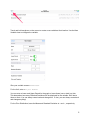
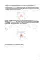
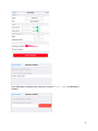
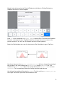
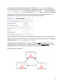
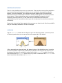
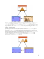
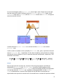
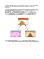
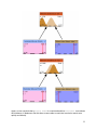
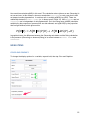
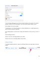
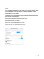
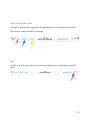
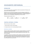
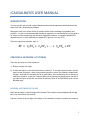
iCAUSALBAYES USER MANUAL INTRODUCTION You can use this app to build a causal Bayesian network and experiment with inferences. We hope you’ll find it interesting and helpful. We expect most of our users will be AI students with a basic knowledge of probability and statistics. You don’t need a deep understanding of regression to use the app but you do need to be aware of some terminology and the basic regression equation: a response variable (RV) depends on one or more explanatory variables (EV) plus an error term (ET). The basic regression equation, then, is: 𝑅𝑉 = 𝐶! 𝐸𝑉! + 𝐶! 𝐸𝑉! + ⋯ + 𝐶! 𝐸𝑉! + 𝐸𝑇 CREATING A NETWORK: A TUTORIAL There are two ways to create a network: 1) Build a network in the app. 2) Create and import an xml file that describes a network. To see the required format, use the app to e-mail a network – either one you build yourself or one of the networks bundled with the app - and open the attached xml file in a text editor. We recommend you use the app to build your networks, as we use a canned XML parser that may not handle typos well, but if you want to import an xml file, e-mail the file and use ‘Open in’ in iPad Mail to open it in the Bayesian app. BUILDING A NETWORK IN THE APP We’ll use the same 3-node throughout this manual. This network comes bundled with the app, but, here, we’ll build it from scratch. Tap the + button at the top right of the home (‘Your Networks’) screen to create a new network. 1 Touch and hold anywhere on the screen to create a new variable at that location. Use the New Variable view to configure the variable. Give your variable a name: Sunscreen. For the Unit, enter Mls per Person. You can enter a Lower and Upper Bound for the graph or leave these (one or both) on Auto, This determines how many Standard Deviations will be displayed for the variable. We’ll leave these on Auto. You can always come back and change this. In fact, you can always come back and change anything! For the Prior Distribution, leave the Mean and Standard Deviation at 0 and 1,respectively. 2 Tap Done on the keyboard and then Done in the top right of the New Variable view. You should see the Sunscreen variable on your screen. The Sunscreen node shows that Mls per Person is approximately normally distributed, with a mean of 0. At this point, this node says, “on average, people use x mls of sunscreen”. Now let’s add another variable. This one is will be an Explanatory Variable for Sunscreen. We’ll call it Melanin Index. This variable is a measure of skin pigmentation, as determined by a reflectometer. For the Unit, we’ll use Index. Again, we’ll leave the Upper and Lower Bounds on Auto. Again, we’ll use the defaults for the Prior Distribution. Position the variables as you like. Use the familiar ‘two finger pinch’ inside a node to make it bigger or smaller or outside to expand or contract the network as a whole. Now, we’ll make Melanin Index an explanatory variable for Sunscreen. Touch and hold inside Sunscreen to edit the variable. In the Edit Variable view, tap Explanatory Variables. 3 In the Explanatory Variables view, swipe left to make Melanin Index an Explanatory Variable. 4 Melanin Index will move from the Potential Explanatory Variables to Existing Explanatory Variables and an Error Term will appear. Enter -0.8 as the coefficient for Melanin Index. Leave the Error Term Mean and Standard Deviation at their default values. Tap Edit Variable in the upper left corner to return to the previous screen. (If you don’t see Edit Variable, tap Done on the keyboard.) Back in the Edit Variable view, you will notice that the Prior Distribution is gone. Tap Done. Now there is an arrow from Melanin Index to Sunscreen. We have changed the meaning of both variables. The arrow indicates that Melanin Index affects Sunscreen use. The coefficient of Melanin Index tells us how: people with a lower Melanin Index use more Sunscreen. This is something a Bayes Net learning algorithm might discover. Our third and last variable will be called Melanoma. For Units, we’ll use Incidence per 100. Once again, we’ll leave Upper and Lower Bounds on Auto. 5 Since we have already created the Explanatory Variables for Melanoma, we can ignore the Prior Distribution and set these up right away. Tap Explanatory Variables, swipe to make both Sunscreen and Melanin Index explanatory variables, and enter -.823 as the coefficient for Melanin Index and -.415 as the coefficient for Sunscreen. We’ll use the Error Term Mean and Standard Deviation defaults here, too. Tap Edit Variable to return to the previous view. (Remember to tap Done on the keyboard first.) Tap Done in Edit Variable. Now we have arrows from Sunscreen and Melanin Index to Melanoma. This is something that might be learned by an ordinary regression analysis, and it says that the incidence of melanoma varies with both Melanin Index and Sunscreen use. Arrange and resize the variables so you can see everything. Save the network if you like and then tap to return to the network view. You might also like to set the Display Options. (You can set Display Options for the network as a whole or for each node individually.) Our small network is complete. 6 OBSERVING AND DOING There is a long-standing controversy over sunscreen. There are those who say that people who use sunscreen end up spending more time in the sun and that the increased sun exposure negates - and even outweighs - any protection sunscreen might provide. Some argue that sunscreen users have lower levels of vitamin D, which protects against skin cancer (as well as other cancers). Others maintain that some sunscreen ingredients increase the risk of melanoma (and other cancers). On the other hand, most dermatologists and cancer organizations say that if you want to reduce your risk of melanoma, you should use sunscreen consistently. Suppose the observational data suggests that sunscreen use doesn’t much affect the probability that you will develop melanoma. Now let’s investigate. OBSERVING Tap the Sunscreen variable with two fingers to put it into Observing mode - you know you are in Observing mode when you see an eye icon in the upper right of the window. A line, representing an observed value, will appear in place of the distribution curve. Leave the other two variables in Graph mode (indicated by a sparkline). Now drag the line around to see the values of the other two variables for a given value of the Sunscreen variable. You will see that the distribution for Melanoma doesn’t move very much. It would seem that Sunscreen use doesn’t much affect the incidence of Melanoma. 7 However, you might also observe something we mentioned earlier when we set up Melanin Index as an explanatory variable for Sunscreen: when Sunscreen goes up, Melanin Index goes down; when Sunscreen goes down, Melanin Index goes up. It appears that people with darker skin use less Sunscreen overall, while people with lighter skin use more; intuitively, this makes sense. So what happens if we observe the effect of different values for Melanin Index? Tap to Observe the Melanin Index variable and drag the observed value line to the left. We are observing values for people with little skin pigmentation. Now drag the line for Sunscreen to the right. It appears that, for people with little skin pigmentation, as Sunscreen usage increases, the incidence of Melanoma goes down. Conversely, as Sunscreen usage decreases, the incidence of Melanoma goes up. 8 Let’s see what happens when Melanin Index has a higher value. Drag the line to the right and then observe the effect of different values for Sunscreen on Melanoma. Again, more Sunscreen means less Melanoma and less Sunscreen means more Melanoma, though the mean has moved to the left. It would seem that Melanin Index is a confound and that Sunscreen use reduces Melanoma rates. It will be useful to consider how the probability of Melanoma (M), given a particular observed value of Sunscreen (S), is calculated. For the sake of simplicity, we’ll pretend we’re dealing with discrete, binary variables. (D and ¬D represent dark skin and light skin, respectively.) The calculation is as follows: 𝑃 𝑀 𝑆) = 𝑃 𝑀 𝐷𝑆)𝑃 𝐷 𝑆 + 𝑃 𝑀 ¬DS)𝑃(¬𝐷|𝑆) DOING We can approach this in another way: instead of Observing what happens with different distributions of Sunscreen and Melanin Index, we can try Doing something so that Sunscreen is not affected by Melanin Index. A real-world analogy would be an experiment or a law that enforced Sunscreen use, regardless of skin pigmentation, so that Melanin Index is eliminated as a confound. Some people will find the idea of a sunscreen law objectionable and anyone who enacted such a law would have to contend with problems related 9 to compliance and enforcement. But never mind all that! This is just a “what if” scenario: What if we enforced sunscreen usage? What if sunscreen use had nothing to do with skin pigmentation? Tap with two fingers a second time to put Sunscreen into Doing mode (indicated by a wrench). Doing means we intervene to fix the value of Sunscreen in such a way that Melanin Index has no effect on it - you will notice that the arrow from Melanin Index to Sunscreen disappears. Now drag the observed value line around: As Sunscreen use goes down, Melanoma increases; as Sunscreen use increases, Melanoma rates go down. Melanin Index is unaffected because we are manipulating Sunscreen use directly; there is no relationship between Sunscreen use and Melanin Index or skin pigmentation. If you perform these manipulations of Sunscreen while Observing different values for Melanin Index, you will notice that, while increased Sunscreen use always lowers melanoma rates, the mean for Melanoma is higher for people with lighter skin and lower for people with darker skin. Melanin Index, in this scenario, has no effect on Sunscreen but it is still a factor when it comes to the observed incidence of Melanoma: The lighter the skin, the greater the susceptibility to Melanoma. However, Sunscreen use always reduces the incidence of Melanoma. 10 Again, we can conclude that Melanin Index is a confound and that Sunscreen use reduces the incidence of Melanoma. But this time we were able to reach that conclusion much more quickly and directly. 11 How would we calculate p(M|S) in this case? The calculation above (where we are Observing) is not correct here. In this scenario, where we manipulate Sunscreen in such a way that it does not depend on skin pigmentation, it would an error to multiply p(M|DS) by p(D|S). There is a relationship between Melanin Index (or, in binary terms, D and ¬D) and Melanoma rate but Sunscreen use is independent of skin pigmentation. So in the Doing case, p(M|DS) should be multiplied by the proportion of persons who are dark-skinned, and p(M|¬DS) by the proportion that are light-skinned, which gives us this: 𝑃 𝑀 𝑆) = 𝑃 𝑀 𝐷𝑆)𝑃(𝐷) + 𝑃 𝑀 ¬DS)𝑃(¬𝐷) In graphical terms, the difference between the Observing calculation and the Doing calculation is the presence (Observing) or absence (Doing) of an arrow between Melanin Index and Sunscreen. MENU ITEMS COLOR AND GRAPHICS To change the display options for a variable, tap and hold, then tap Color and Graphics. 12 Turn Use Network Settings off to over-ride the network settings for this variable. (For network settings, see DISPLAY OPTIONS below.) If you over-ride the network settings, you can: Set the Header Color for the variable. Turn ghosting on or off. When Ghosting is on, the prior distribution for a variable appears as a ‘ghost’ behind any posterior distribution. Set the Display Mode. You can choose to display the distribution as a line (a curve), an area, or both. Select a Background Color. Select a Line Color, if the Display Mode is Line or Both. Select an Area Color, if the Display Mode is Area or Both. DISPLAY OPTIONS To change the display options for a network, tap Display Options in the upper right of the main window. 13 You can: Set the Arrow Display Mode to Simple or Color Coded. If you choose Color Coded, the intensity of the color of an arrow will reflect the strength of the relationship between two variables. Select a Header Color for the variables. Turn ghosting on or off. When Ghosting is on the prior distribution for a variable appears as a ‘ghost’ behind any posterior distribution. Choose to display distributions as lines (curves), areas, or both. . Select a Background Color for the nodes. Select a Line Color, if the Display Mode is Line or Both. Select an Area Color, if the Display Mode is Area or Both. 14 SAVE, SAVE AS, and E-‐MAIL Tap Save or Save As (in the upper left of the main window) to save a network as an xml file. Tap E-mail to e-mail the xml file for a network. HELP Tap the i icon in the upper right corner of the main window to review the gestures described above. 15