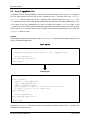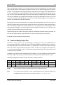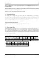
1
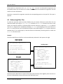
Epp User Manual
Version 1.4.3
Jonas Lippuner, Harry R. Ingleby, Congwu Cui,
David N.M. Di Valentino and Idris A. Elbakri
CancerCare Manitoba
675 McDermot Ave
Winnipeg MB R3E 0V9
Canada
July 2011
The Epp source code and this document are available online at
http://www.physics.umanitoba.ca/~elbakri/epp/
Contact: [email protected]
(Hyperlinks in this PDF may not work properly.)
© 2011 CancerCare Manitoba
Epp User Manual
2
Abstract
Epp (Easy particle propagation) is a user code for the EGSnrc code system (1) to run Monte Carlo simulations of particles propagating through an arbitrary geometry. The photons leaving the simulation geometry can be propagated to a virtual detector, and separate images for primary and scattered photons
can be generated allowing a detailed analysis of the amount and distribution of x-ray scattering. The deposited dose in a voxelized phantom can also be recorded, which makes Epp a viable alternative to the
widely used DOSXYZnrc (2).
Table of Contents
1 Introduction ............................................................................................................................................. 3
1.1 Overview .......................................................................................................................................... 3
1.2 Features ........................................................................................................................................... 4
1.3 License ............................................................................................................................................. 4
2 Installation ............................................................................................................................................... 4
2.1 Requirements................................................................................................................................... 4
2.2 Installing Epp.................................................................................................................................... 4
3 Getting Started with Epp ......................................................................................................................... 5
3.1 Creating an Input File for Epp .......................................................................................................... 5
3.1.1. Defining the Simulation Geometry ...................................................................................... 6
3.1.2. Defining the Simulation Source............................................................................................ 9
3.1.3. Defining the Detector, Simulation Parameters and Other Options...................................10
3.2 Running the Simulation..................................................................................................................11
3.3 Analyzing the Output .....................................................................................................................12
4 Running Epp as a Single Process............................................................................................................12
5 Running Epp in Parallel with Multiple Processes...................................................................................15
6 Input File ................................................................................................................................................15
6.1 Additional Input .............................................................................................................................15
6.1.1. Detector Definition ............................................................................................................16
6.1.2. Dose Calculation.................................................................................................................16
6.1.3. Output Options ..................................................................................................................16
6.2 Referencing Other Files..................................................................................................................17
6.3 Using *.egsphant Files.................................................................................................................18
7 Output Files............................................................................................................................................19
7.1 Photon Output Files .......................................................................................................................19
7.2 Count and Energy Output Files ......................................................................................................20
7.3 Image Output Files.........................................................................................................................21
7.4 Dose Output Files...........................................................................................................................21
8 Version History ......................................................................................................................................22
9 References .............................................................................................................................................24
© 2011 CancerCare Manitoba
July 9, 2011
Epp User Manual
3
1 Introduction
1.1 Overview
Epp is a user code for the Monte Carlo simulation package EGSnrc (1) and can be used to simulate dose
deposition in a voxelized volume and to generate images from an object illuminated by an x-ray source.
The imaging part of the software is designed for analyzing the amount and distribution of Compton and
Rayleigh scattering arising in the imaging process, but can be extended and/or modified to suit other
applications as well.
Epp is written entirely in C++, and based on the EGSnrc C++ class library (3) which provides a wealth of
primitive geometries that can be used to construct a complex simulation geometry. The EGSnrc C++
class library also implements various particle sources and provides a C++ interface to the EGSnrc Monte
Carlo simulation written in MORTRAN.
The actual simulation of the particles propagating through and interacting with matter is done by the
EGSnrc code system. The EGSnrc C++ class library implements the geometry and particle source that the
user has setup and also provides additional functionality for running the simulation in parallel with multiple processes and combining the results of a parallel run. Epp keeps track of the number of scatter
events that a particle undergoes during the simulation and also the dose deposited in each voxel of the
volume in which the user wants the dose to be recorded. In addition to that, Epp also propagates every
photon that leaves the simulation geometry to a virtual detector specified by the user and records the
total number of photons and/or total energy deposited in each pixel. This data can be written to binary
output files and images visualizing the data can also be generated.
For analyzing the amount and distribution of Compton and Rayleigh scatter, the photons are assigned to
one of the following categories for which separate output files can be created; see section 6.3 for more
information:
•
•
•
•
Primary: photons that have not been scattered
Compton: photons that have been Compton scattered exactly once
Rayleigh: photons that have been Rayleigh scattered exactly once
Multiple: photons that have been scattered more than once
The current implementation of Epp does not keep track of other interactions such as pair production or
photoelectric effects, but Epp could be extended to account for these interactions as well. Epp could
also be modified to track other particles.
© 2011 CancerCare Manitoba
July 9, 2011
Epp User Manual
4
1.2 Features
The main features of Epp are the following:
•
•
•
•
•
•
Input file allows referencing other files
*.egsphant files generated by ctcreate can be directly used for simulations
Simulation includes propagation of photons to a virtual detector
Records the total number of photons and the total energy deposited in each pixel of the detector
Results of parallel runs get combined automatically
Output files can be turned on and off individually
1.3 License
Epp is free software; you can redistribute it and/or modify it under the terms of the GNU General Public
License as published by the Free Software Foundation; either version 2 of the License, or (at your option) any later version.
Epp is distributed in the hope that it will be useful, but WITHOUT ANY WARRANTY; without even the implied warranty of MERCHANTABILITY or FITNESS FOR A PARTICULAR PURPOSE. See the GNU General
Public License for more details.
2 Installation
Epp has been designed to run in a Linux environment and has only been tested under Linux. The source
code of Epp is available online at http://www.physics.umanitoba.ca/~elbakri/epp/.
2.1 Requirements
Epp is a user code for EGSnrc and thus requires EGSnrc to be installed and fully configured. This version
of Epp was only tested with EGSnrc V4 2.3.1. EGSnrc can be obtained free of charge from
http://irs.inms.nrc.ca/software/egsnrc/. Since Epp is derived from the EGSnrc C++ class library, the class
library must have been successfully compiled prior to compiling Epp. The EGSnrc C++ class library is part
of the EGSnrc distribution package and should be automatically compiled during the installation process.
2.2 Installing Epp
To install Epp on your Linux system, follow these steps:
1. Download (http://irs.inms.nrc.ca/software/egsnrc/) and install the EGSnrc V4 code system version
2.3.1 and make sure it is fully configured, i.e. all the environment variables are set, this may require
you to logout and login again; note that you need to have a FORTRAN, C and C++ compiler installed
on your system, see the EGSnrc website for more information
© 2011 CancerCare Manitoba
July 9, 2011
Epp User Manual
5
2. Download (http://www.physics.umanitoba.ca/~elbakri/epp/) the Epp source code and extract the
folder Epp into your $EGS_HOME directory (typically egsnrc or egsnrc_mp)
3. Change into the Epp directory, e.g. /home/user/egsnrc/Epp, and run make
If the above steps have all been successfully completed, Epp should now be installed on your system and
ready to be used.
3 Getting Started with Epp
This section describes how to set up a simple input file and for an imaging and a dose simulation and
how to run the simulations. An existing *.egsphant file will be used as the phantom for the dose simulation. It is assumed that EGSnrc and Epp were successfully installed and compiled; see above for the installation instructions of Epp.
This section only provides a very brief introduction to the EGSnrc C++ class library and users not familiar
with the EGSnrc C++ class library are strongly encouraged to have a look at the comprehensive documentation of the class library (3). Epp relies heavily on the EGSnrc C++ class library and the input and
features described in the EGSnrc C++ class library documentation can be directly used in Epp. Epp uses
some additional input elements and features which are described in section 6.
3.1 Creating an Input File for Epp
The input file for Epp (*.egsinp) is a simple text file and organized in key-value and key-subkey pairs.
Anything following a # will be treated as a comment with the exception of two special directives explained in sections 6.2 and 6.3. The following example illustrates the basic syntax for an *.egsinp file.
Example
# a key with a value
key 1 = value
# a key with subkeys
:start key 2:
# a simple subkey with a value
subkey 1 = value
# another subkey with a value
subkey 2 = value
# a subkey with one subkey
:start subkey 3:
subsubkey = value
:stop subkey 3:
:stop key 2:
© 2011 CancerCare Manitoba
July 9, 2011
Epp User Manual
6
Except for the modifications described in section 6, Epp uses exactly the same input as the EGSnrc C++
class library, and the user should refer to that manual (3) for a detailed description of the structure of
the input file as well as the available options.
All numerical values that define a length or coordinates have units centimetre (cm).
3.1.1. Defining the Simulation Geometry
The simulation geometry, i.e. the phantom, is constructed from various geometric primitives like boxes,
spheres, cylinders, cones etc. Those primitives can be rotated, translated and combined with other
primitives. A geometry object, henceforth simply called geometry, is either a single primitive geometry,
a transformation of another geometry or a combination of two or more other geometries. Each geometry is defined with a :geometry: key that contains several subkeys. The subkey name is common to
all geometries and used to assign a name to each geometry by which that geometry can be referenced
later. The name should be unique and cannot contain spaces. The EGSnrc C++ class library documentation (3) describes in detail how the different geometries are defined. Note that by default, all geometric
primitives are centred at the origin.
Each geometry defines one or more regions with a homogenous medium. So in addition to specifying
the geometries that make up the phantom, the user also has to specify the medium for each region.
All geometries are subkeys of geometry definition which will also be referred to as the geometry definition section. This section must contain a single key simulation geometry which
defines which of all the previously defined geometries will actually be used for the simulation. The order
in which the various geometries are defined does not matter. The only restriction is that a geometry has
to be defined before it can be referenced.
The following examples are distributed with Epp and are located in the installation directory of Epp.
Example_
Example_1.egsinp
1.egsinp: Analytical Water Cylinder
This example defines a water cylinder coaxial with the y-axis and with radius 5cm and height 12cm. The
cylinder is then rotated by 45° around the z-axis and embedded into a 15cm air cube. See comments in
the example for additional information.
# all geometries are contained in the geometry definition key
:start geometry definition:
# first we define air hull which is a cube
:start geometry:
library = egs_box
# refer to the class library manual
type = EGS_Box
# refer to the class library manual
box size = 15
# if only one value is specified it will be
# used for all 3 dimensions thus creating a cube
name = air_hull
# we call this geometry object "air_hull"
:start media input:
media = AIR700ICRU # we fill the cube with air
:stop media input:
:stop geometry:
© 2011 CancerCare Manitoba
July 9, 2011
Epp User Manual
7
# next we define a cylinder coaxial with the y-axis and radius 5cm
# NOTE: this cylinder extends indefinitely in +/-y direction
:start geometry:
library = egs_cylinders
type = EGS_YCylinders
radii = 5
name = water_cylinder
:stop geometry:
# to terminate the cylinder, i.e. give it a finite height, we define
# two planes perpendicular to the y-axis at those positions where
# we want to cut the cylinder; so to get a cylinder that is 12cm high
# and centred at the origin we need a plane at y = -6 and one at y = 6
:start geometry:
library = egs_planes
type = EGS_Yplanes
positions = -6, 6
name = y_planes
:stop geometry:
# now we combine the cylinder with the planes to crop it; the NDGeometry
# used here is very powerful but also quite abstract and not necessarily
# intuitive, refer to the EGSnrc C++ class library manual for details
:start geometry:
library = egs_ndgeometry
dimensions = water_cylinder y_planes
name = cropped_cylinder
:start media input:
media = H2O700ICRU
:stop media input:
:stop geometry:
# now we rotate the cropped cylinder by 45 degrees around the z-axis
# the values of the rotation key represent rotation around the x-, y- and
# z-axis in radians, the rotations are applied in the order z, y then x
:start geometry:
library = egs_gtransformed
my geometry = cropped_cylinder
name = rotated_cylinder
:start transformation:
rotation = 0, 0, 0.7854
# angles in radians
:stop transformation:
:stop geometry:
# now we put the rotated cylinder inside the air hull to create our phantom
# NOTE: we can give a list of geometries in the "inscribed geometries" key
# (separated by spaces), but we have to make sure that all inscribed
# geometries are completely contained in the base geometry and don't overlap
:start geometry:
library = egs_genvelope
name = phantom
base geometry = air_hull
inscribed geometries = rotated_cylinder
:stop geometry:
# finally we specify which geometry object should be used for the simulation
simulation geometry = phantom
:stop geometry definition:
© 2011 CancerCare Manitoba
July 9, 2011
Epp User Manual
8
Example_2.egsinp: Voxelized Phantom in Air
This example defines a voxelized phantom imported from an existing *.egsphant file inside an air volume. The voxelized phantom is rotated by 15° around the y-axis.
:start geometry definition:
# first we define air volume which will fill the space between the source
# and the phantom
:start geometry:
library = egs_box
type = EGS_Box
box size = 15, 15, 40
name = air
:start media input:
media = AIR700ICRU
:stop media input:
:stop geometry:
# now we translate the air volume to get it between the source and phantom
:start geometry:
library = egs_gtransformed
my geometry = air
name = translated_air
:start transformation:
translation = 0, 0, -12.5
:stop transformation:
:stop geometry:
# next we import the existing egsphant file phantom_10cm.egsphant which is
# in the same directory as this input file and call it "voxels", the file
# contains a cubic voxelized phantom with side length 10cm
#egsphant voxels phantom_10cm.egsphant
# now we rotate the voxelized phantom by 15 degrees around the y-axis
:start geometry:
library = egs_gtransformed
my geometry = voxels
name = rotated_voxels
:start transformation:
rotation = 0, 0.2618, 0
# angles in radians
:stop transformation:
:stop geometry:
# now we put the rotated voxels inside the air volume
:start geometry:
library = egs_genvelope
name = phantom
base geometry = translated_air
inscribed geometries = rotated_voxels
:stop geometry:
# finally we specify which geometry object should be used for the simulation
simulation geometry = phantom
:stop geometry definition:
© 2011 CancerCare Manitoba
July 9, 2011
Epp User Manual
9
3.1.2. Defining the Simulation Source
There are a few basic source types, like parallel, collimated and isotropic source, which can be used to
define a specific source. The specific sources are constructed from abstract shapes such as, points, lines,
circles, rectangles, boxes etc. Sources can be arbitrarily rotated and translated and multiple sources can
be combined with different weights. The EGSnrc C++ class library documentation (3) describes in detail
what sources and shapes are available and how they are specified in the input file. Note that by default,
all shapes are centred at the origin.
Analogous to the definition of the geometry objects, the source objects are enclosed by :start
source: and :stop source: and all source objects must be inside the source definition section.
The source used for the simulation is defined with the key simulation source.
Example: Collimated Point Source
This example defines a monochromatic point source collimated onto a 15cm by 15cm rectangle which is
perpendicular to the z-axis and located at z = -7.5cm. The point source is located on the z-axis at
z = -32.5cm and radiates 38keV photons. This source is used in both example files.
# all sources are contained in the source definition key
:start source definition:
# we define a new source object which is a collimated source
:start source:
library = egs_collimated_source
name = point_src
# the source shape is the shape that radiates the particles
:start source shape:
type = point
# we use a point as the source
position = 0, 0, -32.5
# shape coordinates of the point
:stop source shape:
# the target shape is the collimator of the source, this is a virtual
# collimator, i.e. there is no leakage
:start target shape:
library = egs_rectangle
# we use a rectangle as collimator
rectangle = -7.5, -7.5, 7.5, 7.5 # x and y coordinates of the upper
# left and lower right corners of
# the rectangle, which is initially
# located at z = 0
:start transformation:
translation = 0, 0, -7.5
# now we translate the rectangle by
# 7.5cm in the negative z direction
:stop transformation:
:stop target shape:
# the spectrum of the source is monochromatic (monoenergetic) with
# energy 38keV
:start spectrum:
type = monoenergetic
energy = 0.038
# the energy is specified in MeV
:stop spectrum:
© 2011 CancerCare Manitoba
July 9, 2011
Epp User Manual
10
# to get a photon source we set the charge of the particles to 0
charge = 0
:stop source:
# finally we specify which source object should be used for the simulation
simulation source = point_src
:stop source definition:
3.1.3. Defining the Detector, Simulation Parameters and Other Options
For an imaging simulation, a detector has to be defined, which is a virtual image plane (100% efficiency).
Every photon leaving the simulation geometry is propagated onto the detector (the medium outside of
the simulation geometry is treated as vacuum) and the total number of photons and/or the total energy
deposited in each pixel of the detector is recorded. The detector is always perpendicular to the z-axis,
see section 6.1.1 for details.
Example_1.egsinp
:start detector definition:
position = 0, 0, 32.5
# coordinates of the centre of the detector
size = 512, 512
# number of pixels in x and y direction
pixel size = 0.1, 0.1
# size of one pixel in x and y direction
:stop detector definition
If the dose in a voxelized volume should be recorded the name of the geometry object in which the dose
should be recorded must be specified. This must be an EGS_XYZGeometry. Note that importing the voxelized volume from an *.egsphant file with the #egsphant directive automatically creates an
EGS_XYZGeometry with the name specified in the #egsphant directive. See section 6.1.2 for details.
Since dose output is disabled by default, it has to be enabled in order for dose output files to be created,
see section 6.1.3 for more information. Furthermore, if no imaging output is desired, it has to be turned
off since it is enabled by default.
Example_2.egsinp
:start dose calculation:
phantom = voxels
# the name of the voxelized volume in which the dose
# should be recorded
:stop dose calculation:
:start output options:
count = n
img-cnt = n
dose = textbin
#
#
#
#
turn off binary photon count output
turn off image photon count output
turn on dose output and specifies that the dose
should be written to a text and a binary file
:stop output options:
© 2011 CancerCare Manitoba
July 9, 2011
Epp User Manual
11
Finally, regardless whether an imaging or dose simulation is run, the user also needs to specify the number of histories, random number seeds and simulation parameters. See section "Summary of transport
parameter" in the EGSnrc Reference Manual (1) for details about the simulation parameters. The following example is used in both example files.
Example
# specifying the number of histories to be simulated
:start run control:
ncase = 10000000
:stop run control:
# specifying the random number generator and initial seed values
:start rng definition:
type = ranmar
initial seeds = 123, 4567
# the two seed values
:stop rng definition:
# specifying the simulation paramters
:start MC transport parameter:
Global ECUT = 0
Global PCUT = 0
Global SMAX = 1e10
ESTEPE = 0.25
XIMAX = 0.5
Boundary crossing algorithm = EXACT
Skin depth for BCA = 0
Electron-step algorithm = PRESTA-II
Spin effects = On
Brems angular sampling = Simple
Brems cross sections = BH
Bound Compton scattering = Off
Pair angular sampling = Simple
Photoelectron angular sampling = Off
Rayleigh scattering = On
Atomic relaxations = On
Electron impact ionization = On
:stop MC transport parameter:
3.2 Running the Simulation
To run the simulation one simply executes the following command in a terminal:
Epp $i Example_1.egsinp $p 700icru.pegs4dat
Section 4 provides detailed information on how to run Epp and the available command line options. The
input file, Example_1.egsinp in the above example, must be located in the Epp user code directory,
i.e. the directory where Epp was installed. It cannot be in any other location or even a subdirectory in
the Epp directory. The PEGS4 file contains the material data used in the simulation and it is specified
with $p. The argument after $p must either be an absolute path to the PEGS4 file or relative to
$HEN_HOUSE/pegs4/data/ or $EGS_HOME/pegs4/data/.
© 2011 CancerCare Manitoba
July 9, 2011
Epp User Manual
12
Epp will display detailed output about the simulation that is running. If an error occurs, Epp displays a
detailed error message. Note that Epp will not run if output from a previous simulation would be overwritten. While the simulation is running, Epp shows the progress in batches, but the displayed result and
uncertainty for each batch will be 0 and 100% respectively because Epp is not recording partial results.
Epp can also be run in parallel mode where the whole simulation is split up among different instances of
Epp. This allows the user to take advantage of multiple CPUs or CPU cores or even a sophisticated distributed computing network. Section 5 briefly explains how to run Epp in parallel, for more details see
section "Running a standard EGSnrc user-code in batch mode" in EGSnrcMP: the multi-platform environment for EGSnrc (4).
3.3 Analyzing the Output
Depending on the specified output options, see section 4 and 6.1.3, Epp creates various output files. A
detailed description of all output is given in section 7; only a brief summary is provided here.
For imaging simulations, the total number of photons and/or the total energy deposited in each pixel
can be recorded by Epp. Individual output files for primary photons, single Compton, single Rayleigh,
multiple scattered photons and all photons can be generated by Epp. Epp can create bitmap images
showing the images on the detector and/or binary files containing the same information. The binary files
can be easily read into other software for further analysis. The structure of the binary files is described
in detail in section 7.2. The file ReadEppOutput.m in the Epp installation directory can be used to read
these output files directly into MATLAB.
Dose output can be written to a text and/or binary file. The structure of those files is described in section 7.4. The text file has the same structure as the text output from DOSXYZnrc. Epp can also create
phase space files containing detailed information about every photon that left the simulation geometry,
see section 7.1 for details.
If Epp was run in parallel, the output of all processes will be combined before any output files are created. The only exceptions are photon output files, as they tend to be very large.
4 Running Epp as a Single Process
Usage:
Epp $i INPUT_FILE $p PEGS_FILE [OPTIONS]
INPUT_FILE is the name of the input file for the simulation; the input file must be in the Epp user code
directory.
PEGS_FILE is the path to the PEGS4 file to be used for the simulation; the path must either be absolute
or relative to $HEN_HOUSE/pegs4/data/ or $EGS_HOME/pegs4/data/.
OPTIONS are additional command line arguments and switches from the list below (optional).
© 2011 CancerCare Manitoba
July 9, 2011
Epp User Manual
13
The following additional command line arguments can be used to change the behaviour of the program:
$o OUTPUT_FILE
$$output OUTPUT_FILE
Sets the base name for the output files to OUTPUT_FILE.
$pr INPUT_FILE
$$parse INPUT_FILE
Epp will parse INPUT_FILE and resolve all #include and #egsphant
directives and create a single completed input file. This is useful to
check and debug #include directives and to create an input file
whose geometry can be viewed with egs_view, as egs_view does
not understand #include and #egsphant.
By default the name of the input file is used.
This option overrides all other options except $h and $$help.
$oP FLAGS
$$output$photout FLAGS
Specifies which photon output files will be created.
FLAGS is any combination of the following letters (any order, without
separators):
•
•
•
•
•
•
•
n: none (turn off all files)
a: all (turn on all files)
p: primary
c: Compton
m: multiple
r: Rayleigh
t: total (sum of p, c, m and r)
Note that n overrides all other flags and a overrides the individual
flags (p, c, m, r, t).
Examples
mcr: only multiple, Compton and Rayleigh files will be created
ptn: no files will be created because n overrides all other flags
an: no files will be created because n overrides all other flags
cart: all files will be created because a overrides all individual flags
The default is n (none).
$oC FLAGS
$$output$count FLAGS
Specifies which count output files will be created.
See above for the description of FLAGS.
The default is a (all).
$oE FLAGS
$$output$energy FLAGS
Specifies which energy output files will be created.
See above for the description of FLAGS.
The default is n (none).
$oIC FLAGS
$$output$img$cnt FLAGS
© 2011 CancerCare Manitoba
Specifies which image count output files will be created.
See above for the description of FLAGS.
July 9, 2011
Epp User Manual
14
The default is a (all).
$oIE FLAGS
$$output$img$e FLAGS
Specifies which image energy output files will be created.
See above for the description of FLAGS.
The default is n (none).
$oD OPTION
$$output$dose OPTION
Specifies that the dose should be recorded in a voxelized geometry
specified in the input file.
OPTION
OPTION is be one of the following:
• text: write dose to text file
• bin: write dose to binary file
• textbin: write dose to text and binary files
Any other value for OPTION will result in no dose output being created.
The default is no value and thus no dose output.
$e PATH
$$egs$home PATH
Sets the EGS_HOME path to PATH instead of the standard path defined
by the EGS_HOME environment variable.
$H PATH
$$hen$house PATH
Sets the HEN_HOUSE path to PATH instead of the standard path defined by the HEN_HOUSE environment variable.
$b
$$batch
Runs the simulation in batch mode, i.e. an *.egslog output file will
be created.
$P N
$$parallel N
Specifies the number (N) of parallel jobs.
$j I
$$job I
Specifies the index (I) of this process in the list of all processes running in parallel.
$s
$$simple$run
Specifies that a simple run control object should be used for parallel
runs. This option is useful if there are issues with locking the run control file otherwise required for parallel runs.
$h
$$help
Prints this message.
This option overrides all other options.
Note that it is not recommended to use the $P and $j command line arguments to run a simulation in
parallel mode, instead the exb script should be used as described in the next section.
Also note that the simulation will not start if the Epp user code directory contains previous output files.
© 2011 CancerCare Manitoba
July 9, 2011
Epp User Manual
15
5 Running Epp in Parallel with Multiple Processes
The simulation can be run in parallel using multiple processes. The easiest method to launch a parallel
run is to use the exb script:
Usage:
exb Epp INPUT_FILE PEGS_FILE p=N
INPUT_FILE is the name of the input file for the simulation; the input file must be in the Epp user code
directory.
PEGS_FILE is the path to the PEGS4 file to be used for the simulation; the path must either be absolute
or relative to $HEN_HOUSE/pegs4/data/ or $EGS_HOME/pegs4/data/.
N is the number of parallel processes that will be run; this number should not be much larger than the
number of available physical processors because there is an overhead cost associated with switching between processes, and thus a larger number of processes will take a longer time to complete.
Note that the switches $i and $p are not present. For more information about exb, one can simply execute exb without any command line arguments.
After submitting a parallel run, the user should check whether the processes are actually running, by using top for example, since it is possible that the simulation failed to start due to a misconfigured input
file, previous output files being present in the output directory or other reasons.
Once all jobs have been submitted and it has been verified that they are running, the user can safely
close the connection to the server and logout. After the last process has finished its part of the simulation, it will automatically combine all the results from the other processes into single output files. When
this is done, the user will be notified by mail (in /var/mail). The mail contains the output from all processes and could provide hints to what went wrong in case the simulation failed to complete.
6 Input File
The input file contains all information required to run the simulation, i.e. the geometry setup, the particle source, the simulation parameters, the detector definition and other parameters.
Except for the modifications described below, Epp uses exactly the same input as the EGSnrc C++ class
library, and the user should refer to that manual (3) for a detailed description of the structure of the input file as well as the available options.
6.1 Additional Input
In addition to the standard EGSnrc C++ class library input, an Epp input file can contain the following additional information. All of the sections must be on the same level as the geometry definition
section.
© 2011 CancerCare Manitoba
July 9, 2011
Epp User Manual
16
6.1.1. Detector Definition
For propagating the photons that left the simulation geometry onto a virtual detector, the input file
must contain the following specifications for the detector:
position
the x, y and z coordinates of the
center of the detector
pixel_size
the size of the individual pixels in cm
in x and y direction
size
the number of pixels on the detector in x and y direction
:start detector definition:
position = 0, 0, 25
pixel size = 0.1, 0.1
size = 512, 512
:stop detector definition:
Note that in the current implementation of Epp, the detector is always perpendicular to the z-axis.
This input is mandatory if any count, energy or image output files should be created.
6.1.2. Dose Calculation
The dose deposited in a voxelized volume, i.e. an EGS_XYZGeometry, can be recorded and written to a
file. This requires that the user specifies the EGS_XYZGeometry in which the dose should be recorded
using the following input element:
phantom
the name of the EGS_XYZGeometry
(as defined in the geometry
definition section or imported
with an #egsphant directive) in
which the dose should be recorded
:start dose calculation:
phantom = my_phantom
:stop dose calculation:
This input is mandatory if any dose output files should be created.
6.1.3. Output Options
The output options can be specified in the input file as follows:
photout
specifies which photon output files
will be created
count
specifies which count output files
will be created
energy
specifies which energy output files
will be created
img-cnt
specifies which image count output files will be created
img-e
specifies which image energy output files will be created
dose
specifies which dose output files will be created
© 2011 CancerCare Manitoba
:start output options:
photout = n
count = a
energy = a
img-cnt = n
img-e = n
dose = text
:stop output options:
July 9, 2011
Epp User Manual
17
These options are equivalent to the $oP, $oC, $oE, $oIC, $oIE and $oD command line arguments and
the possible values are the same as the values for FLAGS with the command line arguments. See the
section 4 for more information.
Note that a command line argument overrides the corresponding option in the input file. This input is
optional.
6.2 Referencing Other Files
To make the input files smaller and more flexible, they can contain references to other files. One can
reference another file using an #include PATH directive. An #include directive can occur at any
place in the input file and also in referenced files; the only restriction is that the #include directive
must be on a separate line. Immediately following #include and extending to the end of the line is
the PATH to the file that is to be included at this point in the referencing file. PATH can be a relative or
absolute path, if it is a relative path, it must be relative to the directory containing the file in which the
#include directive occurs.
Example
The two sample files on the left are in the same directory and result in the input on the right.
input.egsinp
:start geometry definition:
resulting input
#include box.geom
:start geometry definition:
# more geometries
:stop geometry definition:
# more input
box.geom
:start geometry:
library = egs_box
type = EGS_Box
box size = 5, 5, 10
name = my_box
:start media input:
media = water
:stop media input:
:stop geometry:
:start geometry:
library = egs_box
type = EGS_Box
box size = 5, 5, 10
name = my_box
:start media input:
media = water
:stop media input:
:stop geometry:
# more geometries
:stop geometry definition:
# more input
Note that proper indentation is not part of the input syntax and only serves legibility. Also note that it is
the user's responsibility to ensure that no circular references occur.
© 2011 CancerCare Manitoba
July 9, 2011
Epp User Manual
18
6.3 Using *.egsphant Files
*.egsphant files as used by DOSXYZnrc can be directly used with Epp as well. To use an *.egsphant
file in an Epp simulation the user has to put a reference to the *.egsphant file in the geometry
definition section of the input file. An *.egsphant file is referenced with the #egsphant NAME
PATH directive, which will be automatically replaced with the definition of an EGS_XYZGeometry. NAME
is the name of the EGS_XYZGeometry and may not contain any spaces. PATH is the path to the
*.egsphant file from which the EGS_XYZGeometry should be constructed. The path can either be absolute or relative; if it is a relative path, it must be relative to the directory containing the file in which the
#egsphant directive occurs.
Example
The following example demonstrates the use of an #egsphant directive and how Epp translates it into
an EGS_XYZGeometry definition.
input.egsinp
:start geometry definition:
#egsphant my_phantom_name [path to the *.egsphant file]
# more geometries
:stop geometry definition:
# more input
resulting input
:start geometry definition:
:start geometry:
library = egs_ndgeometry
type = EGS_XYZGeometry
name = my_phantom_name
density matrix = [path to the density matrix file]
ct ramp = [path to the ct ramp file]
:stop geometry:
# more geometries
:stop geometry definition:
# more input
Note that the #egsphant directive must be on a separate line and the path of to the *.egsphant file
extends to the end of that line.
© 2011 CancerCare Manitoba
July 9, 2011
Epp User Manual
19
Epp will automatically create the density matrix and ct ramp files based on the *.egsphant file, and will
also remove them after the simulation has successfully finished. The two files will be stored in the Epp
directory under the names NAME.density_matrix and NAME.ct_ramp.
7 Output Files
The photon and imaging results of the simulation are stored in five different types of output files. There
can be up to five files for each type depending on the output options specified with the command line
arguments or in the input file; see sections 4 and 6.1 for more information. Dose output can be stored in
text and/or binary format.
All files of the same type have a different suffix (p, c, m, r, or t) that corresponds to the photon category
primary, Compton, multiple, Rayleigh or total.
In addition to these output files, Epp also creates an *.egsdat file for each process that was run. These
files contain the results of the individual processes and are required to combine the results of all processes at the end of a parallel run. Also, if Epp is executed in batch mode, an *.egslog file containing the
command line output will be created for each process.
7.1 Photon Output Files
The photon output files (*.phot_[p|c|m|r|t].out) contain detailed information about every photon
that has left the simulation geometry travelling in positive Z direction. The information is stored in binary and each photon entry is exactly 32 bytes long. One photon entry consists of eight 4-byte single
precision floating point numbers.
The following diagram illustrates the format of a photon output file:
x
y
z
u
v
w
E
wt
x
y
...
…
float
float
float
float
float
float
float
float
float
float
...
…
first photon – 32 bytes
next photon – 32 bytes
other photons
The eight numbers making up one photon entry have the following meaning:
x, y, z
are the x, y, and z coordinates of the current location of the photon
u, v, w
are the x, y, and z components of a unit vector describing the current direction of travel of
the photon, alternatively these numbers can also be interpreted as the cosines of the angles of the current direction of the photon with the x-, y-, and z-axis
E
is the energy of the photon in MeV
wt
is the statistical weight of the photon
© 2011 CancerCare Manitoba
July 9, 2011
Epp User Manual
20
Due to the way that the EGSnrc C++ class library particle sources are implemented, one cannot simply
count discrete photons on the detector; instead one has to sum the statistical weights of the photons.
Similarly, for recording the total energy deposited in the detector, the energy of each individual photon
has to be multiplied by its statistical weight and then this product will contribute towards the total energy. The sum of the statistical weights or the sum of the energies multiplied by the statistical weights
must then be divided by the average statistical weight of all photons generated by the source. This step
is necessary to obtain meaningful values so that the sum of the statistical weights—even though it is a
fraction—corresponds to the number of photons.
Epp applies this correction automatically to the output files described below, but if the user wants to
read the simulation results from the photon output files directly, the corrections have to be done manually. For this purpose, Epp creates another output file (*.averageWeight.out) containing the overall
average statistical weight as one 4-byte single precision floating point number in binary. This file is only
created if at least one photon output file was created.
Note that Epp does not combine the photon output files of different processes running in parallel. For
each process, different photon output files will be created as specified by the output options.
By default no photon output files will be created.
7.2 Count and Energy Output Files
The count (*.count_[p|c|m|r|t].out) and energy (*.energy_[p|c|m|r|t].out) output files contain the number of photons—actually the sum of the statistical weights as explained above—and the total energy deposited in each pixel of the detector. The information is stored in binary and for each pixel
there is one 4-byte single precision floating point number. The pixels are arranged in row-major order,
i.e. one full row is stored after another. For one row the pixels are stored from left to right and the rows
are stored from top to bottom.
In addition to the data for each individual pixel of the detector, the first eight bytes of the file contain
two 4-byte integers that specify the number of pixels in x direction (columns) and y direction (rows).
The following diagram illustrates the format of a count or energy output file:
Nx
Ny
P(1,1)
P(1,2)
P(1,3)
…
P(2,1)
P(2,2)
P(2,3)
…
...
int
int
float
float
float
…
float
float
float
…
...
4 bytes 4 bytes
first row – Nx ∙ 4 bytes
second row – Nx ∙ 4 bytes
other rows
Nx, Ny
are the number of pixels in x direction (columns) and y direction (rows)
P(i,j)
is the total number of photons or total energy (adjusted sum of statistical weights) that
was deposited in the pixel in the i-th row and j-th column, i = 1 . . Ny, j = 1 .. Nx
© 2011 CancerCare Manitoba
July 9, 2011
Epp User Manual
21
The file ReadEppOutput.m in the Epp installation directory can be used to read these output files directly into MATLAB.
Note that after the last process of a parallel run has finished, the results of all processes are combined
and stored into single count and energy output files.
By default all count and no energy output files will be created.
7.3 Image Output Files
The image count (*.image$count_[p|c|m|r|t].bmp) and image energy (*.image$energy_
[p|c|m|r|t].bmp) output files contain the count and energy on the detector visualized as images. The
pictures are in gray scale with zero photons/energy being black and the highest number of photons/ energy in that category being white. All values in between are linearly scaled.
Note that after the last process of a parallel run has finished, the results of all processes are combined
and stored into single image output files.
By default all image count and no image energy output files will be created
7.4 Dose Output Files
The dose deposited in a voxelized volume, i.e. an EGS_XYZGeometry, can be recorded and written to a
text (*.3ddose) and/or binary file (*.dose.out). The format of the *.3ddose file is exactly the same as
the *.3ddose files created by DOSXYZnrc (2), but unlike DOSXYZnrc, Epp does not normalize the dose
with the incident particle fluence. All values except the first three integers are stored as 8-byte double
precision floating point numbers.
The following diagram illustrates the format of the *.dose.out binary file:
Nx
Ny
Nz
int
int
int
xb(0)
xb(1)
double double
…
…
yb(0)
yb(1)
double double
…
…
zb(0)
zb(1)
double double
…
…
4 bytes 4 bytes 4 bytes x-bounds – (Nx + 1) ∙ 8 bytes y-bounds – (Ny + 1) ∙ 8 bytes z-bounds – (Nz + 1) ∙ 8 bytes
d(0)
d(1)
d(2)
double double double
…
err(0)
err(2)
…
…
double double double
…
dose values – Nx ∙ Ny ∙ Nz ∙ 8 bytes
© 2011 CancerCare Manitoba
err(1)
error values – Nx ∙ Ny ∙ Nz ∙ 8 bytes
July 9, 2011
Epp User Manual
22
The *.3ddose text file has the following format:
Line #
1
2
3
4
5
6
Content
Nx Ny Nz
xb(0) xb(1) ... [Nx + 1 values]
yb(0) yb(1) ... [Ny + 1 values]
zb(0) zb(1) ... [Nz + 1 values]
d(0) d(1) d(2) ... [Nx
Ny
Nz values]
err(0) err(1) err(2) ... [Nx
Ny
Nz values]
Nx, Ny, Nz
are the number of voxels in x, y and z direction
xb(i)
is the i-th voxel boundary in X direction, i = 0 .. Nx
yb(i)
is the i-th voxel boundary in Y direction, i = 0 .. Ny
zb(i)
is the i-th voxel boundary in Z direction, i = 0 .. Nz
d(idx)
is the dose (unit Grays) in the voxel with index idx, idx = 0 .. Nx ∙ Ny ∙ Nz - 1
err(idx)
is the relative error of the dose value in the voxel with index idx, idx = 0 .. Nx ∙ Ny ∙ Nz - 1
idx = x + y ∙ Nx + z ∙ Nx ∙ Ny, where x, y and z are the indices of the voxel in x, y and z direction,
x = 0 .. Nx - 1, y = 0 .. Ny - 1, z = 0 .. Nz - 1
Note that after the last process of a parallel run has finished, the results of all processes are combined
and stored into single dose output files.
By default no dose output files will be created.
8 Version History
Version 1.0.0 Tue 21 Jul 2009
• First stable version with all core features implemented.
Version 1.1.0 Fri 24 Jul 2009
• Added feature for recording deposited energy on the detector.
Version 1.2.0 Mon 31 Aug 2009
• Added support for reading *.egsphant files with the #egsphant directive.
Version 1.2.1 Wed 02 Sep 2009
• Fixed a bug that caused some scattered photons to be falsely labelled as primary photons.
• Fixed a bug that caused a substantial number of primary photons to be falsely labelled as Compton scattered when bound Compton scattering was turned on.
© 2011 CancerCare Manitoba
July 9, 2011
Epp User Manual
23
Version 1.2.2 Tue 03 Nov 2009
• Changed propagation of photons to the detector to remove an offset of the whole image on the
detector.
Version 1.3.0 Fri 20 Nov 2009
• Dropped XML support for input files and regressed to the original EGSnrc C++ Classs Library input
format.
Version 1.3.1 Wed 25 Nov 2009
• Fixed some minor bugs related to the names of the output files and fixed a bug related to importing *.egsphant files from a different directory.
Version 1.3.2 Wed 03 Feb 2010
• Fixed a bug related to running Epp in parallel.
Version 1.4.0 Thu 29 Apr 2010
• Updated to use version 2.3.1 of EGSnrc V4.
• Reduced the changes made to the original EGSnrc C++ class library source code.
• Changed the optimization level to 1 instead of 3 to avoid an artefact that would otherwise show
up on generated images.
• Fixed a bug that prevented the command line arguments $h and $$help from having any effect.
• Introduced a check to make sure that the input and pegs file are specified.
• Added a new command line option $pr or $$parse that parses a given file and resolves all #in$
clude and #egsphant directives, which is very useful to view an input file that uses these directives with egs_view, for example.
Version 1.4.1 Thu 03 Jun 2010
• Fixed bug that falsely labelled some photons as Compton scattered when bound Compton scattering is turned on. This fix was introduced in version 1.2.1, but it got lost.
Version 1.4.2 Fri 06 May 2011
• Fixed a bug that propagated photons to the detector backwards when the photon would not hit
the detector going in its current direction. Now only photons that hit the detector going forward
(in the current direction when they leave the simulation geometry) are scored on the detector.
• Removed restriction that only propagated photons to the detector that were going in the positive
z direction. Now Epp can be used to analyze backscatter as well.
• Fixed phantom_10cm.egsphant, which was an air cylinder inside water instead of a water cylinder inside air.
Version 1.4.3 Sat 09 Jul 2011
• Fixed a bug that did not free some allocated memory.
© 2011 CancerCare Manitoba
July 9, 2011
Epp User Manual
24
9 References
1. I. Kawrakow, E. Mainegra-Hing, D.W.O. Rogers, F. Tessier and B.R.B. Walters. The EGSnrc Code
System: Monte Carlo Simulation of Electron and Photon Transport. Ottawa, Canada : National Research
Council of Canada, 2010. Available online at http://irs.inms.nrc.ca/software/egsnrc/documentation/
pirs701/. NRCC Report PIRS-701.
2. B. Walters, I. Kawrakow and D.W.O. Rogers. DOSXYZnrc Users Manual. Ottawa, Canada : National
Research Council of Canada, 2009. Available online at http://irs.inms.nrc.ca/software/beamnrc/
documentation/pirs794/. NRCC Report PIRS-794revB.
3. I. Kawrakow, E. Mainegra-Hing, F. Tessier and B.R.B. Walters. The EGSnrc C++ class library. Ottawa,
Canada : National Research Council of Canada, 2009. Available online at http://irs.inms.nrc.ca/software/
egsnrc/documentation/pirs898/. NRC Report PIRS-898 (rev A).
4. I. Kawrakow, E. Mainegra-Hing and D. W. O. Rogers. EGSnrcMP: the multi-platform environment for
EGSnrc. Ottawa, Canada : National Research Council of Canada, 2006. Available online at
http://irs.inms.nrc.ca/software/egsnrc/documentation/pirs877/. NRCC Report PIRS-877.
© 2011 CancerCare Manitoba
July 9, 2011