1
SpikeDB Version 1.6 User Manual
McMaster University
Written by Brandon Aubie
http://spikedb.aubie.ca
Contents
1 Introduction
2 User Interface
2.1 Importing Spike Data . . . . . .
2.2 Browse Files List . . . . . . . . .
2.3 Filter Panel . . . . . . . . . . . .
2.3.1 Required Number of Files
2.3.2 X-Variable . . . . . . . .
2.3.3 Tag Filter . . . . . . . . .
2.3.4 Show hidden files . . . . .
2.4 Plots . . . . . . . . . . . . . . . .
2.4.1 General Usage . . . . . .
2.4.2 Spike Raster . . . . . . .
2.4.3 Quick Analysis . . . . . .
2
.
.
.
.
.
.
.
.
.
.
.
.
.
.
.
.
.
.
.
.
.
.
.
.
.
.
.
.
.
.
.
.
.
.
.
.
.
.
.
.
.
.
.
.
.
.
.
.
.
.
.
.
.
.
.
.
.
.
.
.
.
.
.
.
.
.
.
.
.
.
.
.
.
.
.
.
.
.
.
.
.
.
.
.
.
.
.
.
.
.
.
.
.
.
.
.
.
.
.
.
.
.
.
.
.
.
.
.
.
.
.
.
.
.
.
.
.
.
.
.
.
.
.
.
.
.
.
.
.
.
.
.
.
.
.
.
.
.
.
.
.
.
.
.
.
.
.
.
.
.
.
.
.
.
.
.
.
.
.
.
.
.
.
.
.
.
.
.
.
.
.
.
.
.
.
.
.
.
.
.
.
.
.
.
.
.
.
.
.
.
.
.
.
.
.
.
.
.
.
.
.
.
.
.
.
.
.
.
.
.
.
.
.
.
.
.
.
.
.
.
.
.
.
.
.
.
.
.
.
.
.
.
.
.
.
.
.
.
.
.
.
.
.
.
.
.
.
.
.
.
.
.
.
.
.
.
.
.
.
.
.
.
.
.
.
.
.
.
.
.
.
.
.
.
.
.
.
.
.
.
.
.
.
.
.
.
.
.
.
.
.
.
.
.
.
.
.
.
.
.
.
.
.
.
.
.
.
.
.
.
.
.
.
.
.
.
.
.
.
.
.
.
.
.
.
.
.
.
.
.
3
4
4
4
4
4
4
4
5
5
5
5
3 Analysis Plug-In Module
3.1 Basic Usage . . . . . . . . . . . . . . . . .
3.2 Reference . . . . . . . . . . . . . . . . . .
3.2.1 void addOptionCheckbox() .
3.2.2 void addOptionNumber() . . .
3.2.3 void filterSpikesAbs() . . .
3.2.4 void filterSpikesRel() . . .
3.2.5 list getCells() . . . . . . . .
3.2.6 list getFiles() . . . . . . . .
3.2.7 list getFilesSingleCell()
3.2.8 list getOptions() . . . . . .
3.2.9 float mean() . . . . . . . . . .
3.2.10 void plotClear() . . . . . . .
3.2.11 void plotLine() . . . . . . . .
3.2.12 void plotSetLineWidth() . .
3.2.13 void plotSetPointSize() . .
3.2.14 void plotSetRGBA() . . . . . .
3.2.15 void plotXLabel() . . . . . .
3.2.16 void plotXMin() . . . . . . . .
3.2.17 void plotXMax() . . . . . . . .
3.2.18 void plotYLabel() . . . . . .
3.2.19 void plotYMin() . . . . . . . .
3.2.20 void plotYMax() . . . . . . . .
3.2.21 void setPointData() . . . . .
3.2.22 void setPointNames() . . . .
3.2.23 float stddev() . . . . . . . . .
3.2.24 dict ttest() . . . . . . . . . .
3.2.25 void write() . . . . . . . . . .
3.3 Complete Examples . . . . . . . . . . . .
3.3.1 Mean Spike Times . . . . . . . . .
.
.
.
.
.
.
.
.
.
.
.
.
.
.
.
.
.
.
.
.
.
.
.
.
.
.
.
.
.
.
.
.
.
.
.
.
.
.
.
.
.
.
.
.
.
.
.
.
.
.
.
.
.
.
.
.
.
.
.
.
.
.
.
.
.
.
.
.
.
.
.
.
.
.
.
.
.
.
.
.
.
.
.
.
.
.
.
.
.
.
.
.
.
.
.
.
.
.
.
.
.
.
.
.
.
.
.
.
.
.
.
.
.
.
.
.
.
.
.
.
.
.
.
.
.
.
.
.
.
.
.
.
.
.
.
.
.
.
.
.
.
.
.
.
.
.
.
.
.
.
.
.
.
.
.
.
.
.
.
.
.
.
.
.
.
.
.
.
.
.
.
.
.
.
.
.
.
.
.
.
.
.
.
.
.
.
.
.
.
.
.
.
.
.
.
.
.
.
.
.
.
.
.
.
.
.
.
.
.
.
.
.
.
.
.
.
.
.
.
.
.
.
.
.
.
.
.
.
.
.
.
.
.
.
.
.
.
.
.
.
.
.
.
.
.
.
.
.
.
.
.
.
.
.
.
.
.
.
.
.
.
.
.
.
.
.
.
.
.
.
.
.
.
.
.
.
.
.
.
.
.
.
.
.
.
.
.
.
.
.
.
.
.
.
.
.
.
.
.
.
.
.
.
.
.
.
.
.
.
.
.
.
.
.
.
.
.
.
.
.
.
.
.
.
.
.
.
.
.
.
.
.
.
.
.
.
.
.
.
.
.
.
.
.
.
.
.
.
.
.
.
.
.
.
.
.
.
.
.
.
.
.
.
.
.
.
.
.
.
.
.
.
.
.
.
.
.
.
.
.
.
.
.
.
.
.
.
.
.
.
.
.
.
.
.
.
.
.
.
.
.
.
.
.
.
.
.
.
.
.
.
.
.
.
.
.
.
.
.
.
.
.
.
.
.
.
.
.
.
.
.
.
.
.
.
.
.
.
.
.
.
.
.
.
.
.
.
.
.
.
.
.
.
.
.
.
.
.
.
.
.
.
.
.
.
.
.
.
.
.
.
.
.
.
.
.
.
.
.
.
.
.
.
.
.
.
.
.
.
.
.
.
.
.
.
.
.
.
.
.
.
.
.
.
.
.
.
.
.
.
.
.
.
.
.
.
.
.
.
.
.
.
.
.
.
.
.
.
.
.
.
.
.
.
.
.
.
.
.
.
.
.
.
.
.
.
.
.
.
.
.
.
.
.
.
.
.
.
.
.
.
.
.
.
.
.
.
.
.
.
.
.
.
.
.
.
.
.
.
.
.
.
.
.
.
.
.
.
.
.
.
.
.
.
.
.
.
.
.
.
.
.
.
.
.
.
.
.
.
.
.
.
.
.
.
.
.
.
.
.
.
.
.
.
.
.
.
.
.
.
.
.
.
.
.
.
.
.
.
.
.
.
.
.
.
.
.
.
.
.
.
.
.
.
.
.
.
.
.
.
.
.
.
.
.
.
.
.
.
.
.
.
.
.
.
.
.
.
.
.
.
.
.
.
.
.
.
.
.
.
.
.
.
.
.
.
.
.
.
.
.
.
.
.
.
.
.
.
.
.
.
.
.
.
.
.
.
.
.
.
.
.
.
.
.
.
.
.
.
.
.
.
.
.
.
.
.
.
.
.
.
.
.
.
.
.
.
.
.
.
.
.
.
.
.
.
.
.
.
.
.
.
.
.
.
.
.
.
.
.
.
.
.
.
.
.
.
.
.
.
.
.
.
.
.
.
.
.
.
.
.
.
.
.
.
.
.
.
.
.
.
.
.
.
.
.
.
.
.
.
.
.
.
.
.
.
.
.
.
.
.
.
.
.
.
.
.
.
.
.
.
.
.
.
.
.
.
.
.
.
.
6
6
7
8
9
10
11
12
13
15
16
17
18
19
20
21
22
23
24
25
26
27
28
29
30
31
32
33
34
34
.
.
.
.
.
.
.
.
.
.
.
.
.
.
.
.
.
.
.
.
.
.
.
.
.
.
.
.
.
.
.
.
.
.
.
.
.
.
.
.
.
.
.
.
1
Chapter 1
Introduction
Figure 1.1: Main SpikeDB window showing a spike raster and mean spike count analysis plot.
SpikeDB is a database and analysis tool for electrophysiological recordings done with SPIKE (written
by Brandon Warren). It runs on Linux and Mac OS X and Windows. The purpose of SpikeDB is to
provide electrophysiologists with the ability to easily catalogue their electrophysiological recordings for future
analysis. Animals, Cells, and Files can be assigned meta data such as tags to make finding them easier.
Furthermore, all data becomes available in an embedded Python scripting interface to allow for powerful
data analysis without the need to manually export and manipulate the data from SPIKE.
2
Chapter 2
User Interface
A) Filter Panel - Filter the files shown in the Browse Files list.
B) Animal List - List of animals and cells currently imported. Select an animal or a cell by selecting the
arrow head next to each item. Only the selected animals or cells appear in the Browse Files list. Select
All Animals to display all animals, cells and files in the Browse Files list.
C) Browse Files list - A list of files currently selected and filtered.
D) Spike Raster Plot - Displays each spike as a black dot and each stimulus as a line (red = Channel 1,
blue = Channel 2).
E) Quick Analysis Plot - Displays results of the analysis script selected in the drop-down box. There is
a small panel at the very bottom that can be dragged up to view any text outputted by the analysis
script via the print command.
F) File Details Panel - Displays details of the currently selected file and allows the entry of custom data.
G) Cell Details Panel - Displays cell details of the currently selected cell and allows the entry of custom
data.
H) Animal Details Panel - Displays animal details of the currently selected file and allows the entry of
custom data.
3
2.1
Importing Spike Data
SpikeDB uses a database file (SQLite) to store spike data. This means that your SPIKE files are not modified
in any way. Before viewing your SPIKE data in SpikeDB you must create a new database file and then import
the spike files.
1. First select the Create New Database option in the file menu. This file can be named anything
and saved anywhere. For example you could name it MySpikeData.db. If multiple people need to
access this data you could store it on a shared network drive.
2. Click the Save button to create your new database file.
3. Next, select the Import Spike Files option form the file menu and select the directory where
your SPIKE files are located. The import tool will go one level deeper than the directory you select if
needed. Therefore, you could have your SPIKE files in subdirectories of the directory you choose here.
4. Click the Open button after you have chosen the directory with SPIKE files to automatically import
them into SpikeDB. If you have already imported a file, SpikeDB is smart enough to recognize the
duplicate and skip over that file.
2.2
Browse Files List
To view a spike raster and quick analysis plot, click on any file in the list. Multiple files can be analyzed
at the same time by selecting multiple files simultaneously (holding down CTRL on most computers while
selecting files or hold down SHIFT to select a range of files). If a file is considered to be useless (incomplete
recording or incorrect settings for example) then the file can be hidden from view by right clicking on it,
selecting View Details and then checking the Hide file in file list checkbox. As long as the
Show hidden files checkbox in the filter panel is not checked, this file will not be displayed. The file
details window also shows the time when the file was created.
2.3
Filter Panel
The filter panel is used to filter the files shown in the Browse Files window. This can be useful when browsing
your data or when running analysis scripts.
2.3.1
Required Number of Files
Often we are only interested in cells with at least a minimum dataset and thus cells with only 1 or 2 files
recorded are useless. Setting this value to a number greater than 1 will hide any cells that have less than
that number of files recorded for it.
2.3.2
X-Variable
Use this drop-down to filter which types of files are shown based on the file’s X variable.
2.3.3
Tag Filter
Animals and Cells and be given tags in their respective details panels on the right of the window. Only
files that belong to an animal or a cell containing the tag entered in this window they will be shown in the
Browse Files list. Leave blank to not filter on tags.
2.3.4
Show hidden files
Turn this option on to show files in the Browse Files list even if they have been manually marked as hidden.
The hidden files will be tagged with an H to the left of the list when shown.
4
2.4
2.4.1
Plots
General Usage
• Zoom - Left click and drag horizontally to zoom in on a subsection of data.
• View Value - To view the exact value of a data point, hover the mouse cursor over the data point
and the value will appear in the SpikeDB status bar in the bottom left.
• Export Data - Right click anywhere on the plot to bring up the options menu and select Export Data.
This allows you to export the plotted data in CSV files that are ready for import into Excel or for use
in other graphing software such as GLE.
2.4.2
Spike Raster
The spike raster is a built-in plot that displays the stimuli as red (channel 1) and blue (channel 2) lines and
spikes as black dots. Zooming in on this plot will limit the spike times available to the Quick Analysis plot
on the right.
2.4.3
Quick Analysis
By default, this plot will display the mean number of spikes per trial. Other analysis plugins are available
in the drop down box or additional plugins can be loaded by clicking the Open icon. Generally, it is wise to
use plugins that operate on selected files only here as no text display is available. For more general analysis
on many files use the Analysis tab. That said, if multiple files of the same type are selected, the plots can
be overlaid for easy comparison. Click the Advanced button beside the drop down list and check off the
Show Error Bars option to display the error bars in graphs (generally shown as standard deviation).
5
Chapter 3
Analysis Plug-In Module
3.1
Basic Usage
The Analysis Plug-In Module allows you to use the Python scripting language write custom analysis routines
on one or many Spike recording files. Each Python script will have the SpikeDB object available to it and
must contain a function called SpikeDBRun that will be called by SpikeDB when your module is executed1 .
The SpikeDB object provides access to all of the data held within SpikeDB as well as a host of methods
useful for analysis.
The most basic shell of an application will look like the following:
Listing 3.1: Example
def SpikeDBRun():
SpikeDB.print(‘‘Hello World!’’)
Quick Analysis Plugins
Several Quick Analysis plugins are included with SpikeDB and it is easy to add your own. Quick Analysis
plugins are shown in the drop-down box on the Quick Analysis and Analysis toolbars and are defined by
scripts located in the plugins/ folder of the SpikeDB application. The location of this folder depends on your
operating system. Refer to Table 3.1 for details. Quick Analysis plugins function exactly the same way as
Table 3.1: Default plugins folder locations on different operating systems.
Microsoft Windows
Mac OS X
or
Linux
or
C:\Program Files\SpikeDB\plugins\
/Applications/SpikeDB.app/Contents/Resources/plugins/ (built-in)
/Library/Application Support/SpikeDB/plugins/ (user added)
/usr/local/share/spikedb/plugins/ (built-in)
/.spikedb/plugins/ (user added)
other Analysis plugins with two minor differences. First, the name of the plugin to display in the toolbar
drop-down list must be specified on the first line with three # symbols in the format
### Name Goes Here
Second, when retrieving files with the getFiles() method you will generally always want to pass True as
the parameter to ensure that only the currently selected file(s) will be analyzed. When adding new Quick
Analysis plugins to the plugins folder you must restart SpikeDB for them to be available in the drop-down
list.
1 This
requirement was added in SpikeDB 1.5
6
3.2
Reference
All functions listed in this section are accessed via the SpikeDB object. For example, SpikeDB.getFiles(True)
calls the getFiles() method.
7
3.2.1
void addOptionCheckbox(string name,string description,bool default)
Parameters
name
description
default
Variable name for accessing value later.
Name to show in SpikeDB option windows.
Set to True to have the box checked by default.
Description
Call this function in SpikeDBAdvanced() to add a checkbox option to the Advanced options panel.
8
3.2.2
void addOptionNumber(string name,string description,float default)
Parameters
name
description
default
Variable name for accessing value later.
Name to show in SpikeDB option windows.
Default value for this parameter.
Description
Call this function in SpikeDBAdvanced() to add a numerical option to the Advanced options panel.
9
3.2.3
void filterSpikesAbs(float minSpikeTime,float maxSpikeTime)
Parameters
minSpikeTime
Minimum absolute spike time.
maxSpikeTime
Maximum absolute spike time.
Description
Filters the spikes for every file based on the absolute time of the spike in the file.
Listing 3.2: Example
# Have getFiles() only show spikes
# that occured between 10 and 50 ms.
SpikeDB.filterSpikesAbs(10, 50)
10
3.2.4
void filterSpikesRel(float minSpikeTime,float maxSpikeTime)
Parameters
minSpikeTime
Minimum relative spike time.
maxSpikeTime
Maximum relative spike time.
Description
Filters the spikes for every file based on the time of the spike relative to the stimuli onset and offsets. A spike
is included only if it falls within a stimulus onset+minSpikeTime and stimulus offset+maxSpikeTime.
When both channel 1 and channel 2 are active a spike is included if it falls within the relative timing of
either stimulus. To include spikes prior to stimulus onset set minSpikeTime to a value less than zero.
Listing 3.3: Example
# Have getFiles() only show spikes
# that occured 5 ms before and 50 ms after
# a given stimulus.
SpikeDB.filterSpikesRel(-5, 50)
11
3.2.5
list getCells()
Description
A list of dictionary objects is returned where each dictionary object represents a single cell. All cells presently
displayed in the files list on the browse page are always returned. The structure of each dictionary object is
shown in Table 3.4.
Table 3.2: Dictionary structure for each cell in the list of cells returned by getCells().
‘AnimalID’
‘CellID’
‘CarFreq’
‘Depth’
The animal ID where the cell was found.
The ID of the cell.
The cell’s carrier frequency as manually entered in the cell details window.
The cell’s depth as manually entered in the cell details window.
‘Location’
The cell’s location as manually entered in the cell details window.
‘Threshold’
The cell’s threshold as manually entered in the cell details window.
‘ThresholdAttn’
‘TreePath’
‘tags’
The cell’s threshold relative to attenuation as manually entered in the cell details window.
Code used to point to the node in the Cell Selection tree in SpikeDB. Place this into a plotted data poin
A list of tags.
Listing 3.4: Example
# Return a list of all cells in the browse files list.
cells = SpikeDB.getCells()
12
3.2.6
list getFiles(bool onlySelected)
Parameters
onlySelected
When TRUE, only return a list of the files selected in the files list on the browse page.
This is useful when writing a Quick Analysis plugin. When FALSE, return all files
listed on the browse page.
Description
A list of dictionary objects is returned where each dictionary object represents a single file. The structure
of each dictionary object is shown in Table 3.3. Note that a “trial” is a value of a stimulus at a particular
X-variable value. For example, if a file varied the stimulus duration then a trial contains all of the passes for
a particular stimulus duration.
Listing 3.5: Example
# Return a list of all files in the browse files list.
allFiles = SpikeDB.getFiles(False)
# Return a list of selected files in the browse files list.
selFiles = SpikeDB.getFiles(True)
13
Table 3.3: Dictionary structure for each cell in the list of cells returned by getFiles().
‘AnimalID’
The animal ID where the cell was found.
‘CellID’
The ID of the cell.
‘FileID’
The ID of the file.
‘tags’
‘datetime’
‘xvar’
‘speakertype’
A list of tags.
A string in the form YYYY-MM-DD HH:MM:SS of the time the file was created.
String representation of the X variable.
String representation of speaker type.
‘azimuth’
String representation of speaker azimuth position.
‘elevation’
String representation of speaker elevation position.
‘type’
‘duration’
‘attenuation’
‘frequency’
‘begin’
‘trials’
1
Stimulus type (Sinus, Swept Sinus, FM, etc.) on channel 1. Blank if none.
2
Stimulus type (Sinus, Swept Sinus, FM, etc.) on channel 2. Blank if none.
1
Stimulus duration on channel 1. SpikeDB.VARYING if varied.
2
Stimulus duration on channel 2. SpikeDB.VARYING if varied.
1
Stimulus attenuation on channel 1. SpikeDB.VARYING if varied.
2
Stimulus attenuation on channel 2. SpikeDB.VARYING if varied.
1
Stimulus frequency on channel 1. SpikeDB.VARYING if varied.
2
Stimulus frequency on channel 2. SpikeDB.VARYING if varied.
1
Stimulus start time on channel 1. SpikeDB.VARYING if varied.
2
Stimulus start time on channel 2. SpikeDB.VARYING if varied.
List containing dictionary objects defined by:
‘xvalue’
‘duration’
‘attenuation’
‘frequency’
‘begin’
‘passes’
Value of the X variable for this trial.
1
Stimulus duration on channel 1.
2
Stimulus duration on channel 2.
1
Stimulus attenuation on channel 1.
2
Stimulus attenuation on channel 2.
1
Stimulus frequency on channel 1.
2
Stimulus frequency on channel 2.
1
Stimulus start time on channel 1.
2
Stimulus start time on channel 2.
A list of lists of spike times. Each list represents a
14 this stimulus parameter (i.e. in this
different pass over
trial). For example, the ‘passes’ list for a trial with 4
passes could look like [ [23.13,24,9], [22.1], [], [24.22] ].
3.2.7
list getFiles(string animalID,int cellID)
Parameters
animalID
cellID
The animal ID of the desired cell.
The cell ID of the desired cell.
Description
This function operates exactly the same as getFiles() except it returns only those files associated with
the given cell that are listed on the browse page. In general, plugins will be run with all files listed on the
browse page so that all cells are available to the script.
15
3.2.8
list getOptions()
Description
A list of dictionary objects is returned where each dictionary object represents an option by the name given
when addOptionCheckbox() or addOptionNumber() was called in SpikeDBAdvanced().
Listing 3.6: Example
def SpikeDBAdvanced():
SpikeDB.addOptionNumber(’someNumber’,’Enter a number’, 0)
def SpikeDBRun():
options = SpikeDB.getOptions()
print options[’someNumber’]
16
3.2.9
float mean(list values)
Parameters
values
List of numbers to calculate the mean of.
Description
Returns the mean value of all the numbers passed in the values list.
Listing 3.7: Example
vals = [1,2,3,4]
mean = SpikeDB.mean(vals)
print mean
# Output:
#
2.5
17
3.2.10
void plotClear()
Description
Clears the SpikeDB plot and resets the plot variables and style settings. This is called automatically at the
top of each script so generally should not be needed.
Listing 3.8: Example
# Clear the plot
SpikeDB.plotClear()
18
3.2.11
void plotLine(list xValues,list yValues,list errValues)
Parameters
xValues
List of the X values for the (X,Y) points to plot.
yValues
List of the Y values for the (X,Y) points to plot.
errValues
List of the magnitude of the error bars. Enter an empty list for no error bars.
Description
Plot a series of (X,Y) points in the style determined by prior plot setup functions (i.e. plotSetLineWidth,
plotSetPointSize, plotSetRGBA, etc.). The length of xValues and yValues must be the same and
errValues must also be the same length or be empty (i.e. []). In some cases it may not make sense to
plot a point for a particular X value (for example, there is no defined first spike latency for a trial with zero
spikes). In such cases you can assign SpikeDB.NOPOINT to that Y value to produce a disconnected line
missing that point.
Listing 3.9: Example
X = [1,2,3,4,5]
Y = [1,4,SpikeDB.NOPOINT,16,25]
err = [0.5,0.2,0,1.1,0.3]
# Plot the data with error bars
SpikeDB.plotLine(X,Y,err)
# Plot the data without error bars
SpikeDB.plotLine(X,Y,[])
19
3.2.12
void plotSetLineWidth(float lineWidth)
Parameters
lineWidth
The line width connecting points in a plot. Default is 2.
Description
Determines the width of the line when plotting data points for the next call to plotLine(). To remove
lines, use a line width of 0.
Listing 3.10: Example
X = [1,2,3,4,5]
Y = [1,4,9,16,25]
err = [0.5,0.2,0.9,1.1,0.3]
# Remove the line connecting points
SpikeDB.plotSetLineWidth(0)
# Plot the data
SpikeDB.plotLine(X,Y,err)
20
3.2.13
void plotSetPointSize(float pointSize)
Parameters
pointSize
The point size for points in a plot. Default is 8.
Description
Determines the size of point shapes when plotting data points for the next call to plotLine().
Listing 3.11: Example
X = [1,2,3,4,5]
Y = [1,4,9,16,25]
err = [0.5,0.2,0.9,1.1,0.3]
# Use very large points.
SpikeDB.plotSetPointSize(16)
# Plot the data
SpikeDB.plotLine(X,Y,err)
21
3.2.14
void plotSetRGBA(float red,float green,float blue,float alpha)
Parameters
red
Percentage of red between 0 and 1.
green
Percentage of green between 0 and 1.
blue
Percentage of blue between 0 and 1.
alpha
Percentage of alpha between 0 (opaque) and 1 (transparent).
Description
Determine the color of the points and line for the next call to plotLine().
Listing 3.12: Example
X = [1,2,3,4,5]
Y = [1,4,9,16,25]
err = [0.5,0.2,0.9,1.1,0.3]
# Draw in semi-translucent red.
SpikeDB.plotSetRGBA(1,0,0,0.25)
# Plot the data
SpikeDB.plotLine(X,Y,err)
22
3.2.15
void plotXLabel(string xLabel)
Parameters
xLabel
Text to show under the x-axis.
Description
Determine the x-axis label for the next call to plotLine().
Listing 3.13: Example
X = [1,2,3,4,5]
Y = [1,4,9,16,25]
err = [0.5,0.2,0.9,1.1,0.3]
# Set the labels.
SpikeDB.plotXLabel(‘X Value’)
SpikeDB.plotYLabel(‘Squared Value’)
# Plot the data
SpikeDB.plotLine(X,Y,err)
23
3.2.16
void plotXMin(float minXValue)
Parameters
minXValue
Minimum value to show on the x-axis.
Description
Use this function to force the plot to have the x-axis begin at minXValue.
Listing 3.14: Example
X = [1,2,3,4,5]
Y = [1,4,9,16,25]
err = [0.5,0.2,0.9,1.1,0.3]
# Constrain the plot
SpikeDB.plotXMin(2)
SpikeDB.plotXMax(4)
SpikeDB.plotYMin(3)
SpikeDB.plotYMax(17)
# Plot the data
SpikeDB.plotLine(X,Y,err)
24
3.2.17
void plotXMax(float maxXValue)
Parameters
maxXValue
Maximum value to show on the x-axis.
Description
Use this function to force the plot to have the x-axis end at maxXValue.
Listing 3.15: Example
X = [1,2,3,4,5]
Y = [1,4,9,16,25]
err = [0.5,0.2,0.9,1.1,0.3]
# Constrain the plot
SpikeDB.plotXMin(2)
SpikeDB.plotXMax(4)
SpikeDB.plotYMin(3)
SpikeDB.plotYMax(17)
# Plot the data
SpikeDB.plotLine(X,Y,err)
25
3.2.18
void plotYLabel(string yLabel)
Parameters
yLabel
Text to show beside the y-axis.
Description
Determine the y-axis label for the next call to plotLine().
Listing 3.16: Example
X = [1,2,3,4,5]
Y = [1,4,9,16,25]
err = [0.5,0.2,0.9,1.1,0.3]
# Set the labels.
SpikeDB.plotXLabel(‘X Value’)
SpikeDB.plotYLabel(‘Squared Value’)
# Plot the data
SpikeDB.plotLine(X,Y,err)
26
3.2.19
void plotYMin(float minYValue)
Parameters
minYValue
Minimum value to show on the y-axis.
Description
Use this function to force the plot to have the y-axis begin at minYValue.
Listing 3.17: Example
X = [1,2,3,4,5]
Y = [1,4,9,16,25]
err = [0.5,0.2,0.9,1.1,0.3]
# Constrain the plot
SpikeDB.plotXMin(2)
SpikeDB.plotXMax(4)
SpikeDB.plotYMin(3)
SpikeDB.plotYMax(17)
# Plot the data
SpikeDB.plotLine(X,Y,err)
27
3.2.20
void plotYMax(float maxYValue)
Parameters
maxYValue
Maximum value to show on the y-axis.
Description
Use this function to force the plot to have the y-axis end at maxYValue.
Listing 3.18: Example
X = [1,2,3,4,5]
Y = [1,4,9,16,25]
err = [0.5,0.2,0.9,1.1,0.3]
# Constrain the plot
SpikeDB.plotXMin(2)
SpikeDB.plotXMax(4)
SpikeDB.plotYMin(3)
SpikeDB.plotYMax(17)
# Plot the data
SpikeDB.plotLine(X,Y,err)
28
3.2.21
void setPointData(list data)
Parameters
data
List of data values that is the same length as the previous X and Y lists sent to plotLine().
Description
Assigns data values to points previously plotted with plotLine() that SpikeDB can then use. Currently,
assigning this value to a cell’s TreePath (returned in the dictionary from getCells()) is the only supported function. When a point’s data value contains a cell’s TreePath then clicking on that datapoint will
cause SpikeDB to jump to that cell on the Browse page.
29
3.2.22
void setPointNames(list names)
Parameters
names
List of names that is the same length as the previous X and Y lists sent to plotLine().
Description
Assigns names to the points that will be displayed in the SpikeDB status bar when the mouse cursor hovers
over a point.
Listing 3.19: Example
X = [1,2,3,4,5]
Y = [1,4,SpikeDB.NOPOINT,16,25]
err = [0.5,0.2,0,1.1,0.3]
names = [’First’, ’Second’, ’Third’, ’Fourth’, ’Fifth’]
SpikeDB.plotLine(X,Y,err)
SpikeDB.setPointNames(names)
30
3.2.23
float stddev(list values)
Parameters
values
List of numbers to calculate the standard deviation of.
Description
Returns the standard deviation of all the numbers passed in the values list. The function assumes you are
calculating the sample standard deviation and thus the following formula is used:
v
u
N
u 1 X
s=t
(xi − x
¯)2
N − 1 i=1
Listing 3.20: Example
vals = [1,2,3,4]
sd = SpikeDB.stddev(vals)
print sd
# Output:
#
1.66666666667
31
3.2.24
dict ttest(list values1, list values2, bool eqvar)
Parameters
values1
First list of values for t-test.
values2
Second list of values for t-test.
eqvar
Set to True if you believe the two populations have equal variance.
Description
Returns a list of values calculated for a standard t-test.
Table 3.4: Dictionary structure of the return value of ttest().
‘t’
T value.
‘df’
Degrees of freedom.
‘p1’
p-value of a one-tailed t-test (Not implemented).
‘p2’
p-value of a two-tailed t-test (Not implemented).
Listing 3.21: Example
valsA = [1,8,3,5]
valsB = [4,2,1,7]
results = SpikeDB.ttest(valsA,valsB,True)
print results
# Output:
# { ’t’:0.132320752, ’df’:6.0 }
32
3.2.25
void write(string text)
Parameters
text
Text to print to SpikeDB output window.
Description
This function is used internally to print text to the SpikeDB output window and is generally not needed
by analysis script writers. Standard Python output functions like print work just fine and print to the
SpikeDB output window as expected. Errors are also printed to the SpikeDB window.
33
3.3
Complete Examples
3.3.1
Mean Spike Times
Listing 3.22: Calculating the mean spike counts.
### Mean Spike Count
def SpikeDBRun():
# Get selected files only
files = SpikeDB.getFiles(True)
# Plot means for each file.
for f in files:
# Create placeholder lists
means = []
err = []
x = []
# Calculate the mean and standard deviation
# for each trial in the file
for t in f[’trials’]:
# Placeholder for the spike counts
count = []
# Get the X value
x.append(t[’xvalue’])
# Get the spike counts for each pass
for p in t[’passes’]:
count.append(len(p))
# Calculate the mean and standard devations
means.append(SpikeDB.mean(count))
err.append(SpikeDB.stddev(count))
# Plot this file
SpikeDB.plotXLabel(f[’xvar’])
SpikeDB.plotYLabel(’Mean Spike Count’)
SpikeDB.plotLine(x,means,err)
34