Download PC Oscilloscope USB based - Introduction

BACHELOR OF ENGINEERING DEGREE/DEGREE WITH
HONOURS IN ELECTRONIC AND COMMUNICATIONS
ENGINEERING
Final Year Project Report
School of Electronic, Communication and Electrical Engineering
University of Hertfordshire
PC Oscilloscope USB based
Report by
HE, MIAO
Supervisor
Georgios Pissanidis
Date
April 2008
DECLARATION STATEMENT
I certify that the work submitted is my own and that any material derived or quoted from the
published or unpublished work of other persons has been duly acknowledged (ref. UPR
AS/C/6.1, Appendix I, Section 2 – Section on cheating and plagiarism)
Student Full Name: He, Miao
Student Registration Number: 06130352
Signed: …………………………………………………
Date: 07 April 2008
School of Electronic, Communication and Electrical Engineering
BEng Final Year Project Report
ABSTRACT
This report describes a comprehensible method to evaluate desired data in a graphical format
that is a preferable and common way in the communication world. The discussion and
implementation on PC oscilloscope simulation of the graphical data are also involved which
should help reader to have a full and further understanding on this subject.
Using a top level structure diagram-flow chart to introduce the processes of project is a legible
and informative manner. Also, in this report, the aspects and principle of related productions
such as USB port & RS-232 cable is presented. In the end, the test results along with essential
explanations are included as well.
He, Miao / PC oscilloscope USB based
ii
School of Electronic, Communication and Electrical Engineering
BEng Final Year Project Report
ACKNOWLEDGEMENTS
Firstly, I would like to express my thanks to my project supervisor Dr. Georgios Pissanidis for his
patience and intelligible guidance throughout this project.
Also, I hope to thank Talib Alukaidey and Johann Siau for their useful advices.
Finally, I wish to thank my friends for their precious encourage helping me to combat difficulties
during project.
He, Miao / PC oscilloscope USB based
iii
School of Electronic, Communication and Electrical Engineering
BEng Final Year Project Report
TABLE OF CONTENTS
DECLARATION STATEMENT ........................................................................................................i
ABSTRACT .................................................................................................................................... ii
ACKNOWLEDGEMENTS ............................................................................................................. iii
TABLE OF CONTENTS ................................................................................................................ iv
LIST OF FIGURES AND TABLES ................................................................................................ vi
GLOSSARY ................................................................................................................................. viii
1.
Introduction ........................................................................................................................... 1
1.1-Background ......................................................................................................................... 1
1.2- Motivation and challenges ................................................................................................. 2
1.3- Aim and objectives............................................................................................................. 3
1.4- System description ............................................................................................................ 3
1.5- Costing ............................................................................................................................... 4
1.6- Report outline .................................................................................................................... 4
2.
Subject Review ..................................................................................................................... 5
3.
Description of project work ................................................................................................... 6
Chapter 1: Technical theory .......................................................................................................... 6
1.1 Software part: graphics and drawing functionality .............................................................. 6
1.1.1 Windows in the Visual Studio 2005 IDE ...................................................................... 6
1.1.2 The coordinate system of Visual Basic 2005 .............................................................. 7
1.1.3 Graphics operation ...................................................................................................... 7
1.1.4 ActiveX control ........................................................................................................... 10
1.2 Communication between software and hardware ............................................................ 10
1.2.1 The PC‟s Serial Port & Virtual serial port in VB 2005 ................................................ 10
1.2.2 Buffers ....................................................................................................................... 11
1.3 Hardware introduction: RS-232 Cable & DLP-USB245M User Manual ........................... 11
1.3.1 Description of RS-232 cable ...................................................................................... 11
1.3.2 DLP-USB 245M User Manual.................................................................................... 12
Chapter 2: Project development and implementation ................................................................. 14
2.1 Project overview and design ............................................................................................. 14
2.1.1 Project overview ........................................................................................................ 14
2.1.2 Project design ............................................................................................................ 15
2.2 Project implementation ..................................................................................................... 17
2.2.1 Software development ............................................................................................... 18
2.2.2 Integration of the logical sub-flowcharts .................................................................... 32
2.2.3 The function judgment ............................................................................................... 34
2.2.4 Hardware development ............................................................................................. 35
Chapter 3: Testing and debugging .............................................................................................. 38
He, Miao / PC oscilloscope USB based
iv
School of Electronic, Communication and Electrical Engineering
BEng Final Year Project Report
3.1 Test result ......................................................................................................................... 38
3.2 Error analysis .................................................................................................................... 44
3.2.1 Plot data..................................................................................................................... 44
3.2.2 Oscilloscope simulation ............................................................................................. 45
3.2.3 Serial port test ........................................................................................................... 45
Chapter 4: Conclusions and future development ........................................................................ 46
4.1
Project work summary ................................................................................................... 46
4.1.1 Practical outcomes .................................................................................................... 46
4.1.2 Cost and market needs ............................................................................................. 46
4.1.3 Report conclusion ...................................................................................................... 47
4.2
Processes lay out ........................................................................................................... 47
4.3
Difficulties in the procedure ........................................................................................... 47
4.4 Future development ........................................................................................................ 48
4.4.1 Extended / Advanced functions on oscilloscope simulation ...................................... 48
4.4.2 USB connectivity between PC & DSP ....................................................................... 49
REFERENCES ............................................................................................................................ 51
BIBLIOGRAPHY.......................................................................................................................... 53
APPENDICES ............................................................................................................................. 54
APPENDICE A-Software: Source code & Test results ............................................................... 54
APPENDICE B-Hardware: DLP-USB 245M Adapter .................................................................. 70
APPENDICE C-Hardware Accessories: USB cable & Bread-Board .......................................... 72
APPENDICE D-Revised Gantt chart ........................................................................................... 74
He, Miao / PC oscilloscope USB based
v
School of Electronic, Communication and Electrical Engineering
BEng Final Year Project Report
LIST OF FIGURES AND TABLES
Figure 1 Project System ................................................................................................................ 3
Figure 2 Pico Oscilloscope [14] ..................................................................................................... 5
Figure 3 Windows in VB 2005 [3] .................................................................................................. 6
Figure 4 Coordinate System ......................................................................................................... 7
Figure 5 RS-232 D-sub connectors and pin locations for RS-232 connectors [9] ...................... 12
Figure 6 DLP-USB 245M User Manual [10] ................................................................................ 12
Figure 7 Project overview ............................................................................................................ 14
Figure 8 User interface for plotting data ...................................................................................... 15
Figure 9 Serial Port setting .......................................................................................................... 16
Figure 10 Run interface ............................................................................................................... 17
Figure 11 Program structure diagram ......................................................................................... 17
Figure 12 Structure for plotting data ............................................................................................ 18
Figure 13 Step 1: Update array ................................................................................................... 18
Figure 14 Update Array explanation ........................................................................................... 19
Figure 15 (a) step 2.1 draw the border (b) step 2.2 draw the reference table (c) step 2.4 plot
data.............................................................................................................................................. 20
Figure 16 Real oscilloscope screen (left) vs stimulant oscilloscope screen (right) ..................... 21
Figure 17 Sub-flowchart of step 2.4 A) - Call “range_change ()” subroutine .............................. 23
Figure 18 Sub-flowchart of step 2.4 B)-plot data ........................................................................ 23
Figure 19 Sub-flowchart of step 2.4 B) Plot data: draw data using sine function ....................... 25
Figure 20 Integration of each part for step 2 ............................................................................... 26
Figure 21Test serial port ............................................................................................................. 27
Figure 22 Oscilloscope simulation structure ............................................................................... 27
Figure 23 Sub-flowcharts for adjusting amplitude and rescaling size ......................................... 28
Figure 24 Sub-flowcharts for position control “down” (middle) &”up” (right) ............................... 30
Figure 25 Sub-flowcharts for “time/div” control ........................................................................... 31
Figure 26 USB communication with PC ...................................................................................... 32
Figure 27 System flow chart ........................................................................................................ 33
Figure 28 Plot data ...................................................................................................................... 34
Figure 29 Position changes simulation ....................................................................................... 34
Figure 30 9-pin D-type connector (loopback) .............................................................................. 35
Figure 31 USB Bus Powered configuration [10] ......................................................................... 36
Figure 32 Representation of data graphically ............................................................................. 38
Figure 33 Oscilloscope simulation- amplitude changes .............................................................. 39
Figure 34 Special situation of amplitude changes ...................................................................... 39
Figure 35 Oscilloscope simulation-“time/div” .............................................................................. 40
Figure 36 Oscilloscope simulation-“position” control .................................................................. 41
He, Miao / PC oscilloscope USB based
vi
School of Electronic, Communication and Electrical Engineering
BEng Final Year Project Report
Figure 37 Serial port test ............................................................................................................. 42
Figure 38 Different wave-Cos function ........................................................................................ 43
Figure 39 ActiveX control reusable ............................................................................................. 44
Figure 40 Turn analysis ............................................................................................................... 44
Figure 41 Show value analysis ................................................................................................... 45
Figure 42 Reusable user controls .............................................................................................. 45
Figure 43 Processes display ....................................................................................................... 47
Figure 44 Y-POS vs X-POS [11] ................................................................................................. 48
Figure 45 Function generator [11] ............................................................................................... 49
Figure 46 Dual trace .................................................................................................................... 49
Figure 47 Block diagram a digital signal processing system [13] ............................................... 49
Figure 48 Basic connections to a DSP board [10] ...................................................................... 50
Table 1 Cost analysis…………………………………………………………………………………….3
Table 2 Drawline Method [5]…………………………………………………………………………….8
Table 3 Drawstring Method [6]………………………………………………………………………….9
He, Miao / PC oscilloscope USB based
vii
School of Electronic, Communication and Electrical Engineering
BEng Final Year Project Report
GLOSSARY
USB:
Universal Serial Bus
DSP:
Digital Signal Processing /Digital Signal Processor
RS-232: Recommend Standard-232
DAQ:
Data Acquisition
VB:
Visual Basic
COM:
Component Object Model
UART:
Universal asynchronous receiver/transmitter
DTE:
Data Terminal Equipment
DCE:
Data Communications Equipment
FIFO:
First-In, First-Out
VCP:
Virtual COM port
CPU:
Central Processing Unit
MCU:
Micro-programmed Control Unit
VID:
Vendor ID
PID:
Product ID
DAC:
Digital- to-Analogue Converter
GDI+:
Graphics Device Interface +
IDE:
Integrated Development Environment
He, Miao / PC oscilloscope USB based
viii
School of Electronic, Communication and Electrical Engineering
BEng Final Year Project Report
1. Introduction
This section based on feasibility report before contains a brief statement of background
information and system description of the subject, the reasons for undertaking the work, the
aims and objectives and the methods employed to achieve these objectives.
1.1-Background
In modern times, desired data information is frequently analyzed and utilized by people to
develop business, industry and applications in various fields. As time goes on, the
communication and data acquisition system have become core and popular techniques.
Generally speaking, communication is a process that allows human and animals and other
living beings to exchange information by several methods in the world. It exists everywhere by
means of many kinds of forms. Everything takes part in communication must understand a
common language that is transferred with each other. With the development of science and
technology, the ways are used to communicate have also improved.
Modern communication and measurement system designs are increasing in complexity and
functionality as the latest high-performance processors and DSP enable new signalprocessing techniques. What is more, the data transfer becomes much easier than before.
The USB (Universal Serial Bus is a serial bus standard as interface or peripheral equipment
to plug in PC) has got highest data transfer rate up to 8 Mbits/second. Nowadays, the USB
specification is at version 2.0 (Up to 480 Mbit/s (USB 2.0) applications commonly. No matter
what how much data is transferred only with the aid of one cable. In that case it will save
much space cost.
Communication as defined in the RS232 standard is an asynchronous serial communication
method. RS-232 is one of the most widely used techniques used to interface equipment to
computers. It uses serial communications where one bit is sent along a line, at a time. This
differs from parallel communications which send one or more bytes, at a time. The main
advantage of serial communications over parallel communications is that a single wire is
needed to transmit and another to receive. RS-232 is a standard that most computer and
instrumentation companies comply with. [2]
Data acquisition sometimes called DAQ that is the sampling of the real world to generate
data. It may take a variety of forms. At the simplest level, data acquisition can be
accomplished by a person, using paper and pencil, recording readings from a volt meter,
ohmmeter, or other instrument. Personal computers are being used in data acquisition with
special data acquisition boards installed in the computer. These boards are inserted into the
He, Miao / PC Oscilloscope USB based
1
School of Electronic, Communication and Electrical Engineering
BEng Final Year Project Report
chassis of the computer and allow it to be connected to external devices, such as sensors,
probes and other monitoring devices. The computer provides many attractive features to the
data acquisition like high clock speed, programming flexibility, mass data storage and etc. [1]
So, Acquired data always can be displayed, analyzed, and stored on a computer, and using
various general purpose programming languages such as BASIC, C, Java can be developed
for custom displays and control. A specialized programming language used for data
acquisition like the series of Visual Basic which offers a graphical programming environment
optimized and built-in graphical tools and libraries for data acquisition, representation and
analysis.
A data acquisition system is a device designed to measure and logs some required
parameters. To set up a data-acquisition system, the user should know exactly the
characteristics of the desired system, in order to choose the right components in a discerning
way. It is commonly accepted that essential apparatus include analogue measurement
acquisition tool, amplifier, filter, ADC and DAC, and some transmitting and receiving
equipments.
1.2- Motivation and challenges
The communication via USB based without the need for an external power supply and
allowing some devices to be used without requiring individual device drivers to be installed.
Also, it allows devices to be connected and disconnected without restarting the computer.
Therefore, as the improvement of USB, the communication becomes more and more
conveniently and efficiently.
Human prefers to read or analyze the data information in an easier way like present the
desired data graphically. And then the trace presented data may need to amplify, de-amplify
or shift in order to obtain the expected effect.
Although the software development tool-Visual Basic 2005 easily designs great-looking and
easy-to-use applications using an intuitive, drag-and-drop interface designer, it is still a new
programming language hence VB for programming on PC should be a hard and
challengeable work. The communication program between the PC based on virtual serial port
and USB module is still a key issue.
He, Miao / PC Oscilloscope USB based
2
School of Electronic, Communication and Electrical Engineering
BEng Final Year Project Report
1.3- Aim and objectives
Aim:
The aim of this project is to graphically present data acquired over the USB port.
Objectives:
1. Develop the ActiveX control component for the graphical representation of data.
2. Develop the required graphical interface to simulate oscilloscope for presenting the
graphical data to the user.
3. Develop the communication backchannel for acquiring data from the USB module.
1.4- System description
Figure 1 Project System
Figure 1 simply indicates desired system that how to undertake the data exchange between
the PC and USB. In Part 1, the PC is used to install received data and then the GUI window
will be designed to present data in an intuitionistic way by using VB. In part 2, the drivers will
be developed to convert data information from RS-232 to USB and then complete the
communication between the two components. In part 3, USB setting up and the pins‟
connections for powered configuration will be fulfilled. To sum up, this expected system is
composed of software development and hardware configuration to realize graphical
representation desired data.
He, Miao / PC Oscilloscope USB based
3
School of Electronic, Communication and Electrical Engineering
BEng Final Year Project Report
1.5- Costing
Anticipated project costs were generated to ensure that project objectives could be met within
the budget. The initial cost analysis is displayed in Table 1 below:
Equipments
Estimated cost
Remarks
PC
Resource provided by UH
Visual Studio 2005 Software
Download from website:
Software needed for system
Package
http://fsc.feis.herts.ac.uk/
implementation and testing
USB cable (Type A & B)
Around ￡3 ( also available
Hardware accessories
in Final year project lab)
needed for connecting USB
Bread-board
Resource available in lab
adapter
RS-232 Cable
Resource provided by Mr.
Used for testing VCP
John Wilmot
DLP-USB 245 User manual
Resource provided by
Georgios Pissanidis
USB drivers
Download from website:
http://www.dlpdesign.com
Table 1 Cost analysis
1.6- Report outline

Chapter 1: according to literature research, this chapter concentrates on the
related basic theory including the graphics operation and fundamentals and performance
of USB module and RS-232 cable.

Chapter 2: Based on the discussion of chapter 1, it emphasis on the
development of software design for instance how to plot data and how to simulate
oscilloscope‟s functions which are primary work in this project. The hardware
actualization like testing serial port and USB port installation is involved as well.

Chapter 3: The testing and simulation results associated with error analysis
are presented in this chapter.

Chapter 4: The problem and shortcomings have not resolved the
improvements of the project and the difficulties in the procedure are stated. Also, main
progresses are mentioned. Finally, the previous work is concluded briefly as well.
Summary
For what has been discussed above, a generic introduction on this subject including
background information, aim and objectives, the details of cost analysis, and system
description have been introduced. The following section is a review of the history and
background plus the present state of knowledge of the subject area of the project work.
He, Miao / PC Oscilloscope USB based
4
School of Electronic, Communication and Electrical Engineering
BEng Final Year Project Report
2. Subject Review
PC-based oscilloscope (PCO)
Figure 2 Pico Oscilloscope [14]
Although most people think of an oscilloscope as a self-contained instrument in a box, a new
type of "oscilloscope" is emerging that consists of a specialized signal acquisition board
(which can be an external USB or Parallel port device or an internal add-on PCI or ISA card).
PC Oscilloscopes (PCOs) are rapidly replacing traditional digital storage oscilloscopes
(DSOs) as the essential item for custom test equipment arsenal. The major advantages of
PCO are that the display of a traditional oscilloscope is limited by the physical size of the
oscilloscope, and may only be a single colour. With a PC Oscilloscope computer controls the
display, so not only do user get a full colour display, but the display can be the size of user‟s
monitor, projector or plasma display. Also, PC‟s typically have larger and higher resolution
colour displays which can be easier to read. Colour can be utilized to differentiate waveforms.
And USB 2.0 can transfer data at speeds of up to 480 Mbit/s. Using USB 2.0 PC
Oscilloscopes give user incredible performance with fast screen updates and the ability to
stream data. Furthermore, it can be used for data acquisition. [12]
Depending on PCOs‟ capabilities, the prices range from as little as $100 to $2000 therefore it
suits for different customs‟ incomes and needs.
Nowadays, that Pico is the market leader in PC – the modern alternative to traditional benchtop oscilloscopes. Such as PicoScope 2200 Ultra-Compact USB Oscilloscopes is powerful yet
easy to operate. Users benefit from the power of the PC, and the familiar Windows interface
and controls, making the software easy to learn and easy to use on a daily basis. Drivers and
examples are included for LabVIEW, C/C++, Delphi and Visual Basic for integration into
custom applications. [14]
He, Miao / PC Oscilloscope USB based
5
School of Electronic, Communication and Electrical Engineering
BEng Final Year Project Report
3. Description of project work
Chapter 1: Technical theory
Chapter overview:
The background information, the aim and objectives and the structure of the report were
already indicated. In this chapter, the essential information and theory for carrying out the
project is composed of the methods of plotting using Visual Basic language and the general
description of USB port specifics on DLP-USB245M User Manual and RS-232 cable.
1.1 Software part: graphics and drawing functionality
1.1.1 Windows in the Visual Studio 2005 IDE
Figure 3 Windows in VB 2005 [3]
Toolbox: the toolbox contains reusable controls and components that can be added to the
user‟s application. These can range from buttons to data connectors to customized controls.
Design window: the design window is where a lot of the actions take place. This is where
developer will draw user interface on the forms. This window is sometimes referred to the
designer.
Solution explorer: this window contains a hierarchical view of developer‟s solution. A
solution can contain many projects, whereas a project contains forms, classes, modules, and
components that solve a particular problem
Properties: the window shows what properties the selected object makes available. [3]
He, Miao / PC Oscilloscope USB based
6
School of Electronic, Communication and Electrical Engineering
BEng Final Year Project Report
1.1.2 The coordinate system of Visual Basic 2005
When Microsoft first released Visual Basic 1.0 it made building the user interface components
of an application very simple. Instead of having to write thousands of lines of code to display
windows- the very staple of a windows application known as a form that provides a platform
for drawing line, shape or text on the screen. And the computer screen is made up of pixels.
They are very small, but when working together they make a display on the screen. Since
pixels on any given display are always of a uniform size, they are the common unit of
measurement used in computer graphics. Often, the computer screen is set to 1,024 pixels
across and 768 pixels down.
In Visual Basic 6.0, coordinates for forms and controls are expressed in twips while in Visual
Basic 2005, coordinates are expressed in pixels so that the base currency of drawing is the
pixel this means when the mouse is asked for its position, a set of coordinates given in pixels
should be got back. In VB 2005, if the user clicks the mouse in the very top left pixel, the
coordinates of (0, 0) will be shown and the user clicks in the very bottom right pixel, the
coordinates of (1024, 768) will be got back. However, every window has a client area, which
is the area the programmer can use to report the program‟s output. When the lines or shapes
are drawn onto the control or form, the user always dealing with this client area. The
coordinates used when drawing are adjusted so that the position of the window itself on the
screen becomes irrelevant. These coordinates are known as client coordinates. [3]
For example, there are actually two
different coordinates should be got for the
top-left corner of the Form1 paint area.


Around (350,330) is the screen
coordinates, also known as the absolute
position.
Around (0, 0) irrespective of where the
window is positioned on the screen and
this is the adjusted client coordinates,
known as relative position. [3]
Figure 4 Coordinate System
1.1.3 Graphics operation
The graphics class provides methods for drawing objects to the display device. A graphics is
associated with a specific device context and many different shapes and lines by using a
graphics object can be drawn. Before drawing the lines and shapes, render text, or display
and manipulate image, a graphics object that represents a GDI+ drawing surface should be
created. [4] Therefore, there are two steps in working with graphics:
He, Miao / PC Oscilloscope USB based
7
School of Electronic, Communication and Electrical Engineering
BEng Final Year Project Report
Creating a graphics object
A graphics object can be created in a variety of ways:

Receive a reference to a graphics object as part of the
PaintEventArgs in the Paint event of a form or control. This is usually how the
user obtains a reference to a graphics object when creating painting code for a
control.
-Or
Call the „CreateGraphics‟ method of a control or form to obtain a
reference to a Graphics object that represents the drawing surface of that control
or form. Use this method if the user wants to draw on a form or control that
already exists. [4]
After a graphics object was created, using it to draw lines and shapes, render text, or
display and manipulate images.

Draw line: Draws a line connecting the two points specified by the
coordinate pairs. The common form is like Graphics. DrawLine Method (Pen,
Point1, Point2) where the parameters are described in table below:
Parameter name
Type
Pen
Function
System.Drawing.Pen
Determines the color,
width and style of the
line
Point1
System.Drawing.Point
Point structure that
represents the first
point to connect
Point2
System.Drawing.Point
Point structure that
represents the second
point to connect
Table 2 DrawLine Method [5]
Upon the description above how to draw line can be summed as

Creates a pen

Creates points for the endpoints of the line.

Draws the line to the screen.[5]

Draw text: the common method is like Graphics. DrawString Method
(String, Font, Brush, PointF) draws the specified text string at the specified
He, Miao / PC Oscilloscope USB based
8
School of Electronic, Communication and Electrical Engineering
BEng Final Year Project Report
location with the specified Brush and Font objects. The parameters description in
the following table:
Parameter name
type
string
Function
System.string that
String to draw
Represents text as a series
of Unicode characters.
font
System.drawing.font this
Defines a particular format
class cannot be inherited.
for text, including font face,
size, and style attributes.
brush
System.drawing.brush
Determines the color and
texture of the drawn text
Point
System.drawing.pointF
PointF structure that
Represents an ordered pair
specifies the upper-left
of floating-point x- and y-
corner of the drawn text.
coordinates that defines a
point in a two-dimensional
plane.
Table 3 DrawString method [6]

Creates a text string to draw.

Defines the font as Arial (16pt).

Creates a brush to draw with.

Creates a point for the upper-left corner at which to draw the text.

Draws the string to the screen using the font, brush, and destination
point. [6]
Oftentimes, a Graphics object is obtained by handling a control's Control. Paint event and
accessing the Graphics property of the System.Windows.Forms.PaintEventArgs class. The
Paint event is raised when the control is redrawn. It passes an instance of PaintEventArgs to
the method(s) that handles the Paint event. When programming the PaintEventHandler for
controls, a graphics object is provided as one of the PaintEventArgs. [4]
To obtain a reference to a Graphics object from the PaintEventArgs in the Paint event:
1. Declare the Graphics object.
2. Assign the variable to refer to the Graphics object passed as part of the PaintEventArgs.
3. Insert code to paint the form or control. [4]
He, Miao / PC Oscilloscope USB based
9
School of Electronic, Communication and Electrical Engineering
BEng Final Year Project Report
1.1.4 ActiveX control
The history of Windows Forms Controls has roots in something known as controls Visual
Basic Extension (VBX). This later became more widely known as ActiveX, and today,
revitalized and reborn into the .NET Framework, it is known as Windows Forms controls.
There are several good reasons for wanting to create Windows Forms Controls. Firstly, the
same control throughout an application or in lot of different applications can be reusable thus
saving on code and the code relating to a control within the control‟s class can kept for
making the code cleaner and easier to understand. [3]
A user control is implemented as a class. Therefore, anything can be achieved with a class, it
should be also done with a user control that means the user can add properties, methods,
and events to the user control that can be manipulated by whoever is consuming it. The user
control can have two sorts of properties: those that can be manipulated from the properties
window at design time and those that have to be programmatically manipulated at run time.
Hence, in certain circumstances, it is useful to know whether the user control is in design
mode or run mode. The control is in design mode is when a form is being designed and the
properties of the control are being set; it is in run mode when the form is being run and the
control is able to expose methods and events. For example, it is not be appropriate for the
control to plot data when the form is being designed, but the user will want it to when the
application is being run. Usually, a control itself has a Boolean property called DesignMode
which returns true if the control is in design mode and False if it is not. [3]
1.2 Communication between software and hardware
1.2.1 The PC‟s Serial Port & Virtual serial port in VB 2005
All PCs have at least one serial communication port. Serial ports have been a part of the PC
from the beginning. Each COM, or Comm, (communications) port in a PC is an asynchronous
serial port controlled by a UART. A COM port may have the conventional RS-232 interface, or
the port may be dedicated for use by an internal modem or other device. A PC may have
other types of serial ports as well such as USB, Firewire, but these use different protocols and
require different components. Each serial port in a PC reserves a set of port addresses, and
most also have an assigned interrupt-request (IRQ) line, or level. The ports are designated
COM1, COM2, and so on up together with some properties like BaudRate, BitRate and etc. [7]
As for VB2005, it has a control-SerialPort for serial Communication similarly the Mscomm
control in VB6.0. Encapsulation some useful properties (BaudRate, DataBit, Parity,
Encodings….),
methods
(close,
read,
write,
open…)
and
events
(DataReceived,
ErrorReceived...) as SerialPort class and the programming application base on this virtual
serial port. Use this class to control a serial port file resource. This class provides
synchronous and event-driven I/O, access to pin and break states, and access to serial driver
He, Miao / PC Oscilloscope USB based
10
School of Electronic, Communication and Electrical Engineering
BEng Final Year Project Report
properties. [8] The SerialPort VB2005 supported is a communication link between software
and external devices.
1.2.2 Buffers
Buffers are another way that receivers can ensure that they do not miss any data sent to them.
Buffers can also be useful on the transmit side, where they can enable applications to work
more efficiently by storing data to be sent as the link is available. [7]
The buffers may be in hardware, software or both. The serial ports on all but the oldest PCs
have 16-byte hardware buffers built into the UARTs. In the receive direction, this means that
the UART can store up to 16 bytes before the software needs to read them. In transmit
direction, the UART can store up to 16 bytes and the UART will take care of the details of
transmitting the bytes bit by bit, according to the selected protocol. [7]
When the hardware buffers are not large enough, a PC may also use software buffers, which
are programmable in size and may be as large as system memory permits. The port‟s
software driver transfers data between the software and hardware buffers. [7] For this project,
the transferring data must be stressed that in order to achieve maximum throughput,
application programs should send or receive data using buffers and not individual characters.
1.3 Hardware introduction: RS-232 Cable & DLP-USB245M
User Manual
1.3.1 Description of RS-232 cable
RS (Recommend Standard)-232 is one of the most popular computer interfaces of all time
Specifies electrical, functional, procedural and mechanical aspects of the interface and is
designed to handle communications between two devices with a distance limit of 50 to 100
feet depending on the bit rate and cable type. Its most common use is to connect to a modem,
but other devices with RS-232 interfaces include printers, data-acquisition modules, test
instruments, and control circuits. Sometimes, a simple link between computers of any type by
using RS-232 can be achieved. Furthermore, the hardware and programming requirements
for RS-232 are simple and inexpensive and because so many existing devices already have
the interface built-in. An RS-232 link may use any of a number of connector type, pin
configurations and combinations of signals. These days, most PCs use a 9-pin male D-sub
connector for serial ports. These include only the nine signals. Used for connections between
DTEs and voice-grade modems, and many other applications. The Figure 5 shows popular
connectors used in RS-232 interfaces and the pinouts of the connectors. [7]
He, Miao / PC Oscilloscope USB based
11
School of Electronic, Communication and Electrical Engineering
DB-9 Female (DCE)
BEng Final Year Project Report
DB-9 Male (DTE)
Figure 5 RS-232 D-sub connectors and pin locations for RS-232 connectors [9]
The device that connects to the interface is called a Data Communications Equipment (DCE)
and the device to which it connects (e.g., the computer) is called a Data Terminal Equipment
(DTE) which is a device that controls data flowing to or from a computer. In practical terms,
the DCE is usually a modem or other RS-232 device being controlled by a computer and the
DTE is the computer itself, or more precisely, the computer's UART chip. [9]
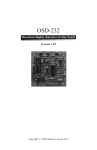
1.3.2 DLP-USB 245M User Manual
Figure 6 DLP-USB 245M User Manual [10]
The DLP-USB245M is the 2
nd
generation of DLP Design‟s USB adapter. This device adds
extra functionality to its DLP-USB1 predecessor with a reduced component count and a new
low price. It has several main features shown below [10]:
He, Miao / PC Oscilloscope USB based
12
School of Electronic, Communication and Electrical Engineering
BEng Final Year Project Report

Send/Receive Data over USB at up to 1M Bytes/sec

384 byte FIFO Transmit buffer /128 byte FIFO receive buffer for high data
throughput

Simple interface to CPU or MCU bus

Protocol is handled automatically within module

FTDI‟s Virtual COM port drivers eliminate the need for USB driver
development in most cases

Integrated Power-on-Reset Circuit

USB VID, PID, serial number and product description

Strings stored in on-board EEPROM

EEPROM programming on-board via USB

Virtual COM port (VCP) Drivers for windows 98/2000 and etc. [10]
The DLP-USB245M provides an easy cost-effective method of transferring data to/from a
peripheral and a host at up to 8 million bits (1-Megabyte) per second. Its simple FIFO-like
design makes it easy to interface to any microcontroller or microprocessor via IO ports.
To send data from the peripheral to the host computer simply write the byte wide data into the
module when TXE# is low. If the (384 byte) transmit buffer fills up or is busy storing the
previously written byte, TXE# is taken high by device in order to stop further data from being
written until some of the FIFO data has been transferred over USB to the host. [10]
When the host sends data to the peripheral over USB, the device will take RXF# low to let the
peripheral know that at least one byte of data is available. The peripheral then reads the data
until RXF# goes high indicating no more data is available to read. By using FTDI‟s virtual
COM Port drivers, peripheral looks like a standard COM Port to the application software. [10]
As for hardware accessories-USB cable & Bread-Board, which are used for installing USB
adapter within Appendix C.
Summary
This chapter introduced the concept and methods of relative theory ready for developing
software design such as how to draw lines and draw text using VB2005. Also, the
fundamental information on hardware devices was presented. After that, the following chapter
will introduce the practical work development for this project based on the theory mentioned
above.
He, Miao / PC Oscilloscope USB based
13
School of Electronic, Communication and Electrical Engineering
BEng Final Year Project Report
Chapter 2: Project development and implementation
Chapter overview
The coordinate system, the method of draw-line and draw text and the features of the RS-232
cable and USB port have discussed above. In this chapter, the project design, the flowchart
instead of source code for describing the implementation of this subject together with some
explanations, the serial port test by using RS-232 cable and the installation of USB module
will discuss in detail.
2.1 Project overview and design
2.1.1 Project overview
Figure 7 Project overview
In the communication world, there is always a need to evaluate data it is preferable for them
to be presented in a graphical format. In order to carry out this aim the subject can be splitted
into five steps as shown as Figure 7. This project should focus on developing software. At the
beginning, a user interface to plot data graphically and adjust the trace presented data in
some ways was built using Windows Forms in the Windows applications and then changed to
create the custom controls known as ActiveX control which is so useful is that they are
reusable. It was Visual Basic programming language that supported main work. When it
comes to step5, USB installation would be done after the communication programme was
ready for receiving data. In the following sections, these five steps will be gone into particulars.
He, Miao / PC Oscilloscope USB based
14
School of Electronic, Communication and Electrical Engineering
BEng Final Year Project Report
2.1.2 Project design
The programming language chosen for the development of software code was Visual Basic
2005 that was a part of Visual Studio 2005. The reason for this based around the advantages
that VB changed the fact of Windows programming by removing the complex burden of
writing code for the user interface (UI). By allowing programmers to draw their own UI, it freed
them to concentrate on the business problems they were trying to solve. Once the UI is drawn,
the programmer can then add the code to react to events. [3]
Figure 8 User interface for plotting data
To build a form or a control, the controls under the Tool-Box are painted onto a blank window
called Forms Designer using the mouse. Each of these controls is able to tell the user when
an event happens. The window as shown above is called “Usercontrol1” by default.
According to Figure 8, the blue colour area for plotting data using the panel control named
“PicDataView” which is a control that contains other controls. It is similar with canvas that can
be used to group collections of controls. If the Panel control's Enabled property is set to false,
the controls contained within the Panel will also be disabled.
On the top of the right side, several controls were designed to undertake the oscilloscope
simulation including labels-provides run-time information or descriptive text for a control,
Buttons-Raises an event when the user click it and texts-enable the user to enter text, and
provides multiline editing and password character masking. [3] For example the amplitude of
the track shown on the left will be zoomed in or zoomed out when the user click the
corresponding buttons. Hence, the three text controls are for showing value of changeable
He, Miao / PC Oscilloscope USB based
15
School of Electronic, Communication and Electrical Engineering
BEng Final Year Project Report
amplitude, time and position and the six buttons are used to control or adjust these events
occurred. The rest part in this figure is for carrying out testing. The two text boxes are for
display the transmission data and receiving data with the button named send data to control
the event happened. Adding another two labels is to describe the controls. On the middle of
the right side, the text box is designed to display the value of last received data.
On the bottom of the user interface, the serial port control selected which is utilized to
undertake the communication channel with the USB module as step 4 shown in Figure 7 and
the other control called OpenFileDialog in case of the windows applications process data from
file therefore an interface is needed to select files to open and save. The .NET Framework
provides the OpenFileDialog & SaveFileDialog classes to do just that. Furthermore, the USB
button on the bottom of right side consists of the serial port settings and the programming for
communication so that another interface was designed:
Figure 9 Serial Port setting
The configuration of serial port such as BaudRate, Parity, DataBits and StopBits was
implemented in this interface and on the right the buttons named “open port” & “close port”
were chosen for controlling the COM port in PCs which was an essential tool for testing serial
port due to different computers often have different COM ports. With this part should make
the system work more conveniently and perfect. The black colour component is regarded as a
sign to indicate the status of the serial port. When the light becomes to red means the port is
close and the green shown the port is open.
Alternatively, from windows 95, it allow the serial port setting to be set by selecting my
computer propertiesDevice MangerPorts (COM and LPT)Port Settings.
After developing the ActiveX control component for plotting data, it still needs an interface as
a platform using the form to execute the function of the existent control called „UserControl1‟
by default.
He, Miao / PC Oscilloscope USB based
16
School of Electronic, Communication and Electrical Engineering
BEng Final Year Project Report
Figure 10 Run interface
Sometimes, more than one user-control is added into this interface called “usercontrol11” and
“usercontrol12” by default to carry out specific task that provides a simple way to contrast and
analyze among different curves. Similarly, the 'Dual trace' oscilloscopes display two V/t
graphs at the same time, so that simultaneous signals from different parts of an electronic
system can be compared. In addition, this interface can be shown to the user in practical work
unlike the ActiveX control before that is just for the designer.
When it comes to the USB port installation, the USB adapter should be inserted into the
bread-board ready for the pin# connections. Then USB port is connected to the PC via a
standard, 6-foot USB cable.
2.2 Project implementation
Figure 11 Program structure diagram
He, Miao / PC Oscilloscope USB based
17
School of Electronic, Communication and Electrical Engineering
BEng Final Year Project Report
2.2.1 Software development
Building a user interface using Windows Forms or Windows Controls is all about responding
to events, so programming for Windows opened up the world of event-driven programming.
Events in this context include, for example, clicking a button, resizing a window, or changing
an entry in a text box. The code that the programmers write responds to these events.
Figure 12 Structure for plotting data
The key task for software development is on plotting data. First of all, adding a new property
to the control is necessary to tell the control when to plot data instead of the globe variable
due to some ineluctable confusion always happened when debugging software.Moreover,
that is a fairly common requirement in writing software is the ability to hold lists of related
data. This functionality can be provided by using an array and it is just lists of data that have a
single data type. When data is coming, the array should be ready for receiving the data and
updating simultaneously owing to the received data is different. From Figure 12, four substeps come under the step2 which are main embranchments for completing to draw the track
representation of desired data with reference table or screen in oscilloscope to measure the
trace onto the canvas-the blue colour part(Figure 8). Next, the flow charts will introduce how
to realize to plot data graphically step by step based on Figure 12.
Step1: Add new Property & Update the array
Figure 13 Step 1: Update array
He, Miao / PC Oscilloscope USB based
18
School of Electronic, Communication and Electrical Engineering
BEng Final Year Project Report
To add a new property called “data”, a member variable-“idata” should be declared in the
public class loop as integer for storing a value. When the value is changed, it will call into the
object and set the property. When the property is set, the text in the private member that was
just defined needs to be set as well. After that, the new property will be exposed when the
project is built.
The explanation on Figure 13 (a)

Define coming data: a variable-“idata” working through the algorithm for the
coming data is declared that can be passed to the default value of an empty integer for
the data property.

DesignMode: if the property is a fairly simple type such as String, Integer, or
Boolean and does not have parameters, it can be manipulated at design mode. If the
property is a complex object, such as a database or file connection, or if it has parameter,
it should be carried out at run time. [3] Obviously, this property has a parameter and the
„DataUpdate‟ event should be active at run mode, hence, at run time the property is
manipulated and raise the event named „DataUpdate‟.

RaiseEvent: „DataUpdate‟: the user own events from the control named
„DataUpdate‟ should be exposed that is allowed the custom who use this control to take
action in their code when the event is raised. Defining the „DataUpdate‟ event is as
simple as adding an Event statement, the event name, the parameters that the event will
return. In this case, the new event-„DataUpdate‟ is performed to updating the array to
store the “idata”. To raise an event, the RaiseEvent statement needs to be specified, the
event name-„DataUpdate‟ as well as the parameters for the event being raised should be
passed to it together.
The exposition on Figure 13 (b):

Update „idata‟ to array: The array ready for plotting called m_DataPlot (1000)
is defined as integer in the Public Class loop and 1000 means 1000 locations for holding
data. Therefore, the received data need to be taken into this data array. The „m_DataPlot‟
array should allocate room to hold “idata” as the Figure 14 shown. To realize this function,
the counter named „iDataCounter‟ was defined as a variable to alter and control the
length of the „m_DataPlot‟ array. After several cycles, the location of m_DataPlot (0)
would be empty for storing the received data-“idata”.
Figure 14 Update Array explanation
He, Miao / PC Oscilloscope USB based
19
School of Electronic, Communication and Electrical Engineering

BEng Final Year Project Report
Text-Box show: from Figure 8 the design interface, on the middle of right
side the text control is designed to display the last value-„idata‟ to the user. In that case,
the user can be aware of the value of received data.

Refresh method: refreshes the content of the table. This might be necessary
after a call to a method when the page does not automatically reflow.
Step 2: Draw reference table & plot data
This step is divided into four sub-steps those are step 2.1 draw the border of region for
plotting or reference table, step 2.2 draw the divisions used to measure the curve like the
background screen of oscilloscope, step 2.3 draw texts for showing value and step 2.4 plot
data using sine math function.
Step 2.1
Step 2.2
Step 2.4
Start
Start
Define the range
Define offset
Start
Create graphics
object “gr”
of reference
table
Define four
points
Calculate every
Divide the
step or scaling of
plotting region by
10
X axis: dx
Or
Draw the border
of table
Draw lines from
left to right & from
End
A). Call
“range_change
()” subroutine
top to bottom
B). Plot data
End
End
Figure 15 (a) step 2.1 Draw the border (b) step 2.2 Draw divisions (c) step 2.4 Plot data
He, Miao / PC Oscilloscope USB based
20
School of Electronic, Communication and Electrical Engineering
BEng Final Year Project Report
The description on Figure 15 (a):
The function of a real oscilloscope is extremely simple: it draws a V/t graph, a graph of
voltage against time, voltage on the vertical or Y-axis, and time on the horizontal or X-axis.
As shown as Figure 16 (left), the screen of this oscilloscope has 8 squares or divisions on the
vertical axis, and 10 squares or divisions on the horizontal axis. Usually, these squares are
1 cm in each direction. [11]

Create graphics object “gr”: when to draw line, text or shape, a graphics
object named “gr” represents a GDI+ drawing surface should be created first by using to
call the „CreateGraphics‟ method of a control or form to obtain a reference to a Graphics
object.

Define four points: the border of region was designed as a rectangle that
was composed of two pairs of height and width consequently the four coordinates points
need to be defined at the proper position according to the screen-“PicDataView” shown
as below:
Figure 16 Real oscilloscope screen (left) vs stimulant oscilloscope screen (right)
For example, the width and height of “PicDataView” can be found like:
m_endY=PicDataView.height & m_endX=PicDataView.width
Therefore the coordinate of P1 may be defined as (70, 5), P2 (70, m_endY-20), P3
(m_endX-10, m_endY-20) and P4 (m_endX-10, 5).

Draw the border of table: four lines connecting every two points specified by
the coordinates by using gr. Drawline (Pen, Point1, Point2) format can be drawn where
the “pen” is chosen to determine color or style of the line.
The explanation on Figure 15 (b):

Define the range of reference table: For what has been discussed above, the
reference table was designed as rectangular so that height and width can be utilized to
determine the range of it. On account of this, the range of reference table:
He, Miao / PC Oscilloscope USB based
21
School of Electronic, Communication and Electrical Engineering
BEng Final Year Project Report
Height=P2Y-P1Y = m_endY - m_startY - 25
Likewise:
width = m_endX - m_startX – 80 where the m_startY and m_startX are
defined as 0 initially.

Divide the plotting region by 10: from Figure 16, the „region A‟ was framed
to be separated into 10 squares or divisions on the vertical axis, and 10 squares or
divisions on the horizontal axis. Such as:
m_Vnum=height/10 & m_Hnum=width/10 where the m_Vnum and m_Hnum figure every
divisions of the screen which is prepared for next step.

Draw lines from left to right & from top to bottom: two “for” loops and the
gr. Drawline method to carry out this step is the best way. On this condition, the key is
about using a variable along with the m_Vnum or m_Hum to draw lines at different
positions. When the lines are drawn from left to right, the variable multiplies the m_Vnum
that means adding a distance of square towards y axis every time, the “pen” will draw a
line. As time goes by, when the 9 cycles of loop complete, nine lines will appear in the
horizontal direction of region A. Then the same way to draw lines from top to bottom but
the variable should multiply the m_Hnum that describes the “pen” will draw a line as
adding a distance of square towards x axis shown as Figure 16(right).
The further description on Figure 15 (c):

Define offset: the globe variable „offset‟ is defined to use for vertical midpoint
that ensure the track representation of data is drawn from the middle of the reference
table. Ideally, it should be calculated as the height of “PicDataView” minus the half of
height of reference table. This variable is so useful that will discuss in detail in the
following section.

Calculate every step of “x” axis-dx: the resolution of x axis or the step of x
will be used in the “plot data” part. It depends on the width of reference table and the
length of array hold the data. Therefore, it is defined as:
dx = width/ m_DataPlot.lenght-1 sometimes it is called scaling.
width = m_endX - m_startX – 80 and „m_DataPlot‟ is the array ready for
Where
plotting both of them have been already introduced above.

Call “range_change ()” subroutine: the subroutine called “range_change()”
is the scaling of y axis or the resolution of between unit pixel in the region of window
display that will be added in the “plot data” part as well. This part consists of a subflowchart will be described minutely below.

Plot data: after the data acquiring over the USB module and then storing in
the „m_DataPot‟ array, it should be plotted onto the reference table graphically by using
the sine math function. This section includes several sub-flowcharts which will be
discussed in the following part.
He, Miao / PC Oscilloscope USB based
22
School of Electronic, Communication and Electrical Engineering
BEng Final Year Project Report
Start
At the beginning, user can define two parameters to
express the amount of data which intend to show
Define the
amount of data to
currently in the y axis such as m_MaxValue (1000)
display: „m_range‟
and m_MinValue(-1000) thereby:
m_range = m_MaxValue - m_MinValue
And the other correlative parameter is the height of
The region of
reference table that is:
display window:
Height = m_screen_range = m_endY - m_startY –
m_screen_range
25 where the m_screen_range is the range of
display window in y axis or the display region in the
dy
window of data display. Hence, the scaling of y axis
=m_screen_range/
is:
m_range
dy = m_screen_range / m_range or
Height/ m_range .
End
Figure 17 Sub-flowchart of step 2.4 A) - Call “range_change ()” subroutine
2.4B) Plot data
2.4B) Plot data: “for loop”
Start
Start
i =0 to
Define current
coordinates point:
m_DataPlot.length1
x1=m_startx+70
Define y1, x2 & y2
Start
Use “for loop”
Restrict the sine
Y1&y2?
x1=x2
wave in the plotting
Draw data using
No
region
sine function in
Limit y1&y2
No
run interface
in the region
Use
gr.drawline(x1,
End
Yes
x2, y1, y2)
Use
gr.drawline(x1, x2,
y1, y2)
End
Figure 18 Sub-flowchart of step 2.4 B)-plot data
He, Miao / PC Oscilloscope USB based
23
End
School of Electronic, Communication and Electrical Engineering
BEng Final Year Project Report
The explanation on 2.4 B) plot data in Figure 18:
There are three primary steps for plotting data. First of all, the x-dimension(x1) of the current
coordinates point should be defined outside the „for‟ loop. Secondly, using „for‟ loop is to
realize the circle for drawing sine wave. Besides, at the Form Designer for “plotting data”
(Figure 10), the data should be plotted.
The exposition on 2.4 B) plot data: “for” loop:

i=0 to m_DataPlot.length -1: the “i” is defined as a counter and adding 1 as
the loop cycles every time so that it can be utilized to execute together with the ydimension (y1) of the current coordinates point and the following coordinates point (x2,
y2) owing to the distance or displacement of x axis and y axis should increase
automatically along with the length of „m_DataPlot‟ array increases for drawing sine track.
Moreover, the “i” is the parameter of „m_DataPlot‟, thus, the m_DataPlot (i) describe the
needed data not the address.

Define y1, x2 & y2: on this condition, the “offset”, “dx”, “dy” were introduced
above should be performed together with these variable. The y-dimension of the current
point is calculated ideally :
y1 = offset - m_DataPlot (i) * dy
But in the practical debugging, some unknown problem occurred, if the y1 was defined as
above shown, the track would always turn over that would discuss in the following
chapter. Accordingly, the y1 is corrected to
y1 = offset + m_DataPlot (i) * dy
Likewise, the next coordinates is defined as
x2 = 71 + i * dx (x1=70)
y2 = offset + m_DataPlot (i + 1) * dy
The “offset” is to assure the begging point is at the middle of the reference table so all
coordinates points are plotted according to the “offset”. If the “offset” changes, the
position of the curve will be altered as well. By multiplying the “dx” and “dy”, the sinecurve can be zoomed in and zoomed out automatically as the size of screen changes.
Assuming the “dx” or “dy” are not used the curve will be only straight line in the x axis or y
axis.

Restrict the sine wave in the plotting region (note: Y1&y2 stands for y1&y2 belong to
the plot region):
When the sine wave is zoomed in, the trace may be beyond the reference table therefore
„if‟ statement should be used to test the conditions about the value of y1 and y2. If both of
them are in the region of reference table, the statement of drawing line will be executed
directly. On the contrary, they should be forced to the maximum value of y1 and y2 and
then the next statement will be performed as well.
He, Miao / PC Oscilloscope USB based
24
School of Electronic, Communication and Electrical Engineering

BEng Final Year Project Report
Using gr. drawline (x1, y1, x2, y2): hundreds or thousands of related
coordinates points or data come into being a track like sine wave. And in order to plot
data by using sine function, the points in the coordinates system have to be moved
forward through some track. Accordingly, the x1 should be forced to x2 and then the loop
will be back to the start that drives the loop continues to cycle until all the data hold in the
„m_DataPlot‟ array is drawn out.
The programming language of this part should
2.4B) Plot data: draw
data using sine function
be developed in the Code Editor for the required
interface to the user (Figure 10) the counter “t”
cannot be less than the locations or the amount
of data stored in the „m_DataPlot‟ array. In that
Start
case, it does not waste the room of the plotting
region and vice versa. And then the existent
Define “t” as
counter
control called “usercontrol1” as a common
control will appear under the project toolbox that
should be added to the “plotting form”. After that,
the “usercontrol1” becomes “usercontrol11” in
fact both of them are the same. At the step 1,
Add “usercontrol1”
the public property called “data” has already
to form of plotting
added to the “usercontrol1” that is used to tell
data
the control when to plot the data instead of the
variable. In addition, the sine function is defined
as sin (_Byval a as double) as double where “a”
Usercontrol11.data ()
is an angle measured in radians so it must be
=500 * Math.Sin(Math.PI
multiplied by PI/180 to convert degrees to
* t / 500)
radians. Therefore, the statement for plotting
can be written:
Usercontrol11.data= 500 * Math. Sin (Math. PI *
End
t / 500) where “500” is the amplitude and
because the m_DataPlot is designed to allocate
1000 locations at the beginning, “/500” is one
period of the sine wave.
Figure 19 Sub-flowchart of step 2.4 B) Plot data: draw data using sine function
He, Miao / PC Oscilloscope USB based
25
School of Electronic, Communication and Electrical Engineering
BEng Final Year Project Report
Integration of each
part for step 2
Start
“PicDataView” like the canvas that is designed to
Define panel
display all the lines or text or shapes so that its height
/canvas region
and width should be defined as a reference parameter
for other components.
Draw the border
The reference table or the background screen of
of plotting region
oscilloscope is utilized to measure the
amplitude, time or the position of the track has
plotted on the canvas. The text is drawn which is
Draw the
used to show value clearly.
reference
table/divisions
Draw text
The screen as a two-dimensional graph of one or more
Plot data using
electrical potential differences (vertical axis) plotted as
sine math
a function of time or of some other voltage (horizontal
function
axis).
End
Figure 20 Integration of each part for step 2
Every related part for plotting data and drawing the reference table can be encapsulated into
an independent subroutine named “DrawData” for example that will be make the program
work efficiently and conveniently to call in the oscilloscope simulation section. And because of
the programming for Windows is commonly known as event-driven programming, the
subroutine ”DrawData” must be called in the „paint‟ event which is provided by the control
itself and raised when the control is redrawn. Also, the data to be plotted should be happened
in the run mode not the design mode.
He, Miao / PC Oscilloscope USB based
26
School of Electronic, Communication and Electrical Engineering
BEng Final Year Project Report
The virtual serial port that is provided by the Visual Basic 2005 is used to perform the serial
communication. It is also can be said it becomes a link between the programming language
and the external device-USB module. So the testing is a necessary procedure during the
project implementation. The flow chart on testing serial port is shown below:
Double click the “send” button in the
design interface of “Usercontrol1”
which converts to Code Editor Mode
and call “SPDataSend” subroutine
that is edited to execute the function
of serial port. The key component is
when to tell the serial port to send
data or receive data therefore, the „if‟
statement is called to tell conditions
for serial port open or close. When
the serial port is open, the program
writes the data to the buffer of serial
port using SerialPort1.Write method.
In other words, the serial port sends
the data to the buffer. The received
data can then be retrieved from the
buffer
by
a
function
called
SerialPort1.Read. This step should
work together with the RS-232 cable
that will discuss in the following
section. Eventually, if the transmitted
data can be received over the serial
port that proves the serial port is
working and vice versa.
Figure 21Test serial port
Until now, the first objective on the graphical representation of data specific on plotting data
using Active X control have completed . Many controls of the oscilloscope allow user to
change the vertical or horizontal scales of the V/t graph, so that it can display a clear picture
of the signal user want to investigate. The following procedure is the oscilloscope simulation.
The general components can be designed as following illumined:
Figure 22 Oscilloscope simulation structure
He, Miao / PC Oscilloscope USB based
27
School of Electronic, Communication and Electrical Engineering
BEng Final Year Project Report
According to Figure 22, actually, rescaling the control size in the run interface does not belong
to the oscilloscope simulation and it is used when the user wants to observe and analyze
more than one control in the interface as Figure 10 shown. Hence, designer should guarantee
all the functions of the controls still working as expected. As for the amplitude, position and
time, in the practical operation they are common controls of an oscilloscope therefore the aim
of this part is to simulate their function. The flow chart listed below for every part will go into
particulars:
Figure 23 Sub-flowcharts for adjusting amplitude and rescaling size
The explanation on “amplitude” control:

Process the m_MaxValue & m_MinValue: As mentioned in plotting
data part, the “m_MaxValue” & “m_MinValue” can be defined to describe the amount
of data intended to show which determine the scaling of y axis- “dy”. Furthermore, the
“dy” is used to define the y-axis of current point y1 & the next point y2 in the sine
wave. On account of this, if the amplitude of the curve intends to be altered, the
corresponding parameter “m_MaxValue” & “m_MinValue” should be updated as well.
For instance, assuming multiply them by 1 as a reference level thus, the sine wave
should be multiplied by 1.1 to zoom in and multiplied by 0.9 to zoom out. However,
when it is zoomed in after several times, it will be drawn outside the reference table
so that the source code should be developed to restrict the trace as Figure 18 shown
above.
He, Miao / PC Oscilloscope USB based
28
School of Electronic, Communication and Electrical Engineering

BEng Final Year Project Report
Refresh method: the „refresh‟ is utilized to avoid the variable
overlapping of the amplitude.

Call plotting data subroutine: this subroutine points to the
“DrawData” mentioned above that includes about drawing reference table and plotting
data. When click the “zoom in” or “zoom out” control the track will disappear if the
“DrawData” subroutine is not called.
The description on rescaling size:
Only at the design mode, the control in the run interface named “usercontrol11” (Figure 10)
can be rescaled the size and ideally, the control size can be changed to any standard. But the
size has to be specified a minimum value logically for all the controls can be visible in the
screen. Since there are many controls need to be defined the position according to the size of
“usercontrol11” that can be found by using the „resize‟ event which indicates using the width
or height property can set the window width and height independently. On this condition, a
reference position such as the position of “PicDataView” (Figure 8) should be defined by the
width and height of the “usercontrol11” first. And then the position of another controls added
in the “usercontrol11” can be defined based on the “PicDataView”.
When it comes to altering the position of the sine wave, the flow charts in next page indicate
that it goes down and goes up separately. Adjusting Y-POS allows the zero level on the Yaxis to be changed, moving the whole trace up or down on the screen to give an effective
display of signals like pulse waveforms while do not alternate between positive and negative
values of x axis.
He, Miao / PC Oscilloscope USB based
29
School of Electronic, Communication and Electrical Engineering
Start
BEng Final Year Project Report
Start
Start
Call “downdata” or
No
Offset<
“Updata” subroutine
Offset>100
(m_endY-100)
Yes
Yes
Calculate the
average step of
position changes
Counter:
Counter:
i_stepdown_count=i_
i_stepup_count=i_ste
stepdown_count+1
pup_count+1
Show value
Vary position according
Vary position according
to counter
to counter
Refresh
method
Update
Update
“offset”
“offset”
Set counter:
Set counter:
i_stepup_count=0
i_stepdown_count=0
End
End
End
Figure 24 Sub-flowcharts for position control “down” (middle) &”up” (right)
The discussion on the “downdata” subroutine in Figure 24 (middle) (nearly the same as
“updata” subroutine):

Offset< (m_endY-100): m_endY equals to the height of the “PicDataView”.
Using the „if‟ statement is to avoid the sine wave disappear from the region for plotting.

Counter: i_stepdown_count =i_stepdown_count+1: i_stepdown_count is
defined as a counter to adjust the position and it will be added by 1 as the “down” button
is clicked every time automatically so that it is also a necessary variable for calculating
the magnitude of position changes.
He, Miao / PC Oscilloscope USB based
30
School of Electronic, Communication and Electrical Engineering

BEng Final Year Project Report
Vary the position according to counter: actually, the value of position
changes are ready for updating the “offset” that is based on the “i_stepdown_count”.

Update the “offset”: if “offset” changes, initially it is in the middle of the
reference table, all of the related points will remove together that result in the track will
move as well. Additionally, the “offset” must be determined by both of up and down
position changes to avoid jumping steps that means when the curve needs to go up or
go down from the current position.

Set the counter: i_stepup_count =0: after adjusting the curve to go down,
the other counter “i_stepup_count” must be set to zero that is because this statement is
used to avoid jumping steps due to whenever finishing the “up” function and converting
to the “down” button the other counter should be added from start. Simply speaking, the
two counters for controlling the curve to go up and go down must be independent from
each other. ( in the following section of function
judgment
will discuss this point
graphically)
Figure 25 Sub-flowcharts for “time/div” control
After finishing the oscilloscope simulation, the second objective on developing the required
graphical interface like oscilloscope for presenting the graphical data to the user has almost
come true. So, the next part is about the third objective to develop the programming for
communication between the USB and PC. The flow chart can be designed as following:
He, Miao / PC Oscilloscope USB based
31
School of Electronic, Communication and Electrical Engineering
BEng Final Year Project Report
Figure 26 USB communication with PC
2.2.2 Integration of the logical sub-flowcharts
Referring to Figure 27 below, additional description should be listed as the following:

COM Port configuration: as mentioned in the project design section (Figure
9), the programming for realization the serial port setting including the initialization and
configuration of Ports‟ name, BaudRate, Parity, DataBits and StopBits by using an
independent interface should be performed. Then it connects with the main interface
over “USB” button (Figure 8).

Add new property: in the practical condition, when the custom intend to
change some property of user controls but considering that they are not allowed to
control the design interface (Figure 8) and only have access to the run interface (Figure
10), adding new property to the control is a desired function. And then in the Properties
window, it will appear under the existent control category. In that case, the custom can
change some property optionally for instance the background of the screen or the line
color of the sine wave depends on themselves.

Install USB: as a matter of fact, the installation of USB is about the hardware
development including the powered configuration and USB driver installation.

Develop programme for communication: when this step have been ready
for communicating, some corresponding parts will be updated together.

Offset: as for transforming position, time or amplitude, this key variable have
to be changed from local to globe type.
He, Miao / PC Oscilloscope USB based
32
School of Electronic, Communication and Electrical Engineering
BEng Final Year Project Report
Start
Design user
interface
COM Port
Add new
configuration
Property
No
Serial Port
available?
Yes
Test serial Port
No
Data
send/receive?
Yes
Add property &
Update array
Plot data
Oscilloscope
Figure 27 System flow chart
simulation
Develop programme
for communicating
Install USB
End
He, Miao / PC Oscilloscope USB based
33
School of Electronic, Communication and Electrical Engineering
BEng Final Year Project Report
2.2.3 The function judgment
2.2.3 a) plot data
Generally speaking, to plot data graphically should process the following procedures:
Storing data in the array
Reading data from array
Plotting data using math function
Commonly using 2- dimension-x, y to express the pixel or coordinates point that make up of
the track drawn in the screen. Sine Y-dimension stands for the data from array, all of them
should be drawn out one by one for plotting shown as table below. It is the counter that
defined to control reading data. Also, the plotting is a durative process and all points in the
track can be only described as the current point and the following point. Hence, the points
should go ahead that can be driven by x1equals to x2. Finally, the math function is called to
manage these relative points so that the plotting is working successfully.
Figure 28 Plot data
2.2.3 b) oscilloscope simulation
When it comes to the “position” control, there are two important parameters to drive it to work
as expected.
Figure 29 Position changes simulation
He, Miao / PC Oscilloscope USB based
34
School of Electronic, Communication and Electrical Engineering
BEng Final Year Project Report
As figure above shown, when the curve goes up twice at point ① and then goes down must
be from this current position not the initial position to avoid jumping steps. Therefore, in the
programming design, there was a parameter defined to record this position added to the
calculation of “offset”. If the curve goes down from point ① to point ② and then need to go
up again, the other parameter also can be said the counter for controlling the trace to go up
should be forced to zero because the counter always record the last position, in that case,
when click the “up” button the curve will go up to the top of screen straight. Following this
point, the system can execute as expected.
As for “time/div” control, the project does not work perfectly because the sine wave can be
only adjusted the amount of periods has drawn in the window not the locations of array for
plotting. Maybe the reason is that the resolution of x axis has not been considered or some
variables need to be declared as globe not local.
Another disadvantage on this system is that the communication backchannel between the
USB and PC still exist some problem due to the serial port cannot read all of data from the
buffer array if the statement “serialport.read” is only used that result in it just read the last
received data in array. Hence, only single data can be read from buffer not a set of data
received from USB.
2.2.4 Hardware development
2.2.4 a) using RS-232 cable to test serial port
Refer to the “pinout” of RS-232, the pin#2 describes the received data and pin#3 describes
the transmitted data. When using single PC to communication, the Female (DCE) end of the
cable should be hanged and then the pin#2 and pin#3 should be connected together that
forms a loop to transmit and receive data. When the serial port in PC was open and then
clicked the “send” button, the data written to the buffer would be send out and then went back
to the PC via RS-232.
Figure 30 shows the main RS-232 connection for 9-pin connections without hardware
handshaking. The loopback connections are used to test the RS-232 hardware and software.
The program on testing part used a loopback on the TD/RD lines so that a character sent by
the computer will automatically be received into the receiver buffer. This set-up is useful in
testing transmit and receive routines. The character to be sent is entered via the keyboard. [2]
Figure 30 9-pin D-type connector (loopback)
He, Miao / PC Oscilloscope USB based
35
School of Electronic, Communication and Electrical Engineering
BEng Final Year Project Report
2.2.4 b) the installation of DLP-USB245M User manual
During this step, there are two sub-steps should be undertaken.

USB adapter Powered configuration

The installation of USB driver
The bread-board, USB cable and DLP-USB245M User manual could be used together to
carry out the installation. As stated in Appendix C, the bread-board connects components
together to build circuits and the leads of most components can be pushed straight into the
holes in the board. The USB cable could be used as a connector between the USB port and
PCs. The type “B” usually connected to the DLP-USB245M and the other end “A” connected
to a conventional host hub (Figure 11). As shown the pin configuration (Figure A-1), the pin#1
& pin#4 of the cable describes the power supply –specification 5V and pin#2 & pin#3 are for
transmitting and receiving data. After plugging the USB into bread-board, the circuit
connections to supply power according the Figure below shown had to be completed.
Figure 21 illustrates a typical USB bus powered
configuration. A USB Bus Powered device gets
its power from the USB bus. Basic rules for USB
Bus power devices are as follows –
a) On plug-in, the device must draw no more
than 100mA
b) On USB Suspend the device must draw no
more than 500uA.
c) A Bus Powered High Power Device ( one that
draws more than 100mA ) should use the
SLEEP# pin to keep the current below 100mA
on plug-in and 500uA on USB suspend.
d) A device that consumes more than 100mA
cannot be plugged into a USB Bus Powered
Hub
e) No device can draw more that 500mA from
the USB Bus.
f) The power descriptor in the EEPROM should
be programmed to a value of zero. [10]
Figure 31 USB Bus Powered configuration [10]
Based on the DLP-USB 245M pinout description (see the Appendix B), pin#3 should connect
with pin#10, pin#11 and pin#12 respectively which supply 5V power to USB. The pin#13
should connect with pin#14 that provides handshaking signal RXF# and TXE# to transmit and
receive data.
He, Miao / PC Oscilloscope USB based
36
School of Electronic, Communication and Electrical Engineering
BEng Final Year Project Report
The USB driver is necessary component for DLP-USB 245M working with PCs. The following
step on installing the USB driver [10]:
1. Download the DLL version of the device drivers from either dlpdesign.com or ftdichip.com.
Unzip the drivers onto a blank floppy disk or into a folder on the hard drive.
2. Download the serializer program from either dlpdesign.com or ftdichip.com. Unzip the
package and place it in a folder on the hard drive.
3. Connect the DLP-USB245M board to the PC via a standard, 6-foot USB cable. This action
initiates the loading of the USB drivers. When prompted, select the folder where the DLL
version of the device drivers were stored in step one. Windows will then complete the
installation of the device drivers for the DLP-USB245M board. The next time the DLPUSB245M module is attached, the host PC will immediately load the correct drivers without
any prompting.
4. Run the serializer program and write the VID (0403), PID (6001), a description string of the
users‟ choosing and manufacturers ID as instructed in the instruction manual that was
downloaded with the serializer software. Terminate the serializer program and disconnect the
DLP-USB245M board from the USB cable. Wait 10 seconds and reconnect the DLPUSB245M board. Reboot the PC if instructed to do so. [10]
After installing the driver, under the “Device Manager” of PCs the “USB serial port (COM port)
and USB serial converter would appear automatically. That means the USB driver can
retrieve COM ports from the system and automate the selection of COM port to the height
available. The USB serial port also can be said as Virtual COM ports that is a link between
the programming language or software development and USB module.
Summary
This chapter introduced the project implementation consists of programme development and
USB port installation. The previous one utilized several logic flow chats to describe how to
plot data and how to realize the oscilloscope simulation. As for hardware development, mostly
referred to the data sheet of the DLP-USB 245M user manual to perform how to plug the USB
into PCs.
Indubitably, the following chapter should lay out the testing results together with required
explanation.
He, Miao / PC Oscilloscope USB based
37
School of Electronic, Communication and Electrical Engineering
BEng Final Year Project Report
Chapter 3: Testing and debugging
Chapter overview
After discussing the project design and implementation together with the analysis of function
judgement, this chapter will present the testing results including the tack and oscilloscope
functions shown and different waves display using some common math models. Also, error
analysis depends on the results shown will be involved.
3.1 Test result
Figure 32 Representation of data graphically
Using sine function with proper parameters defined such as amplitude and period, the correct
sine wave was drawn on the plotting region-“PicDataView”. The texts in the screen were
designed to measure amplitude, position and time of the curve. The “offset” had emphasized
before was working as expected. The graph was restricted to draw from the vertical midpoint
that made it looked like more symmetrical and convenient to scale. The “last value” displayed
the last data in array abstractly. In addition, the parameter in the sine function must be
defined larger than the locations of array. If it is only the half of the locations, the half of the
sine wave will appear that results in waste of room. Adding two controls in user interface is a
convenient way to analyze the two graphs. (See Appendix A)
He, Miao / PC Oscilloscope USB based
38
School of Electronic, Communication and Electrical Engineering
BEng Final Year Project Report
The following two pictures show the amplitude changes:
Figure 33 Oscilloscope simulation- amplitude changes
When clicked on the “zoom in” button, the amplitude increased as the magnitude decreased
that was because the specification of this coordinates system was (0, 0) at the top-left of the
screen. Likewise, the wave zoomed out as the magnitude increased in Figure 33.
The figure on the left
indicates the curve may
be drawn outside the
reference table when it is
zoomed in. luckily, the
programme have already
compiled for erasing the
redundant lines.
Figure 34 Special situation of amplitude changes
He, Miao / PC Oscilloscope USB based
39
School of Electronic, Communication and Electrical Engineering
BEng Final Year Project Report
Figure 35 Oscilloscope simulation-“time/div”
On this condition, the “time” control was designed to change the periods of sine wave drawn.
And the texts on the left of x axis determine the horizontal scale of the graph which appears
on the oscilloscope screen. For example, With 10 squares across the screen and the spot
moving at 0.628 s/DIV that is 0.62831 * 10 = 6.2831≈ 2π. The period of the curve can be
calculated. At the same time, the amplitude can be altered as well depend on users
themselves. In fact, for this project the “time” control means the locations of array changes
for plotting in that case, the realization of function here is not exactly that will particularize in
the error analysis part.
He, Miao / PC Oscilloscope USB based
40
School of Electronic, Communication and Electrical Engineering
BEng Final Year Project Report
The Y-POS control allows user to move the spot up and down the screen. For the present,
adjust the trace so that it runs horizontally across the centre of the screen.
Figure 36 Oscilloscope simulation-“position” control
The variable “offset” is the most important factor for controlling the position changes and it
must be changed to define as the globe variable. If “offset” is still the local variable, when
using another controls like amplitude with the “position” simultaneously, the sine wave will go
back to the original position not currently. Also, the “offset” here must be related to the “offset”
of the data are plotted part. Likewise, the amplitude or the periods can be transformed as well.
Like adjusting the VOLTS/DIV and TIME/DIV until a clear picture of signal can be obtained.
However, the corresponding numerical value is not exactly, in particular, when the curve goes
up or goes down continuously.
He, Miao / PC Oscilloscope USB based
41
School of Electronic, Communication and Electrical Engineering
BEng Final Year Project Report
Figure 37 Serial port test
According to the project implementation, there are there steps for testing:

Connect RS-232 with PCs

Click on “USB” button

Select required COM Port and open it ( the alert light show green)

Write the random value in the “transmit string” text box

Click on the “send” button
Afterwards, from Figure 37 above, the written number disappears from the “Transmit String”
box and then the same value appear in the “Receive String” that proves the test is successful.
He, Miao / PC Oscilloscope USB based
42
School of Electronic, Communication and Electrical Engineering
BEng Final Year Project Report
Figure 38 Different wave-Cos function
By changing the math function, the different trace can be achieved. In the same way, the
amplitude or position of cos wave also can be changed shown as Figure 38 above. Actually,
from the “last value” shown that records the first point in the track therefore, according to the
math function, the sine wave should be zero while the cos wave should be 500. But when
adding the “timer” control in the user interface, with the help of programming language the
“last value” is mutative and durative number which also can be used to simulate the received
data from external devices such as USB module.
Other waves also can be achieved by using different math function for instance: Truncate Sqrt,
Tan or Round and etc. (see Appendix A)
He, Miao / PC Oscilloscope USB based
43
School of Electronic, Communication and Electrical Engineering
BEng Final Year Project Report
Figure 39 ActiveX control reusable
Adjusting the size of each control to ensure all controls could be visible and usable in the run
interface. Also, these two traces could be altered the amplitude or position within Appendix A.
3.2 Error analysis
3.2.1 Plot data
Theoretically, the “offset” should minus the data derived from the array when calculate the ydimension of the current and next point (y=offset-m_DataPlot (i)*dy). However, in that case,
the curve shifted abnormally as shown below:
Figure 40 Turn analysis
The reason of the curve on the left happened is that in the “update array “part, the array is
updated from the bottom of array (m_DataPlot.Length - 1 To 1 Step -1) not from the top
results in the order of plotting data should be from maximum value to minimum (t = 1000 To 0
Step -1) when using the sine function and vice versa. When both of them were provided with
the correct corresponding relationship, the expected result would lay out (right). Alternatively,
changing the equation -y=offset-m_DataPlot (i)*dy to y=offset+m_DataPlot(i)*dy is also a
solution.
He, Miao / PC Oscilloscope USB based
44
School of Electronic, Communication and Electrical Engineering
BEng Final Year Project Report
3.2.2 Oscilloscope simulation
When the “up” and “down” button
were clicked continuously, the value
for explaining the position changes
was not correct any more (329). That
is because the “offset” displacement
does not respond to the show value.
Figure 41 Show value analysis
When added two controls in the run
interface, from figure left, there was
just waveform no other controls
anymore although the size rescaling
had adjusted. Back to Figure 39 that
was an updated design interface
over readjusting the controls‟ size
and position, this was not an
expected step. The improvement is
that the programming on recalling
size has to be correct. Maybe, more
than one reference positions should
be utilized to define the controls‟
positions and size.
Figure 42 Reusable user controls
3.2.3 Serial port test
When using the RS-232 cable to test port, oftentimes the “send” button had to be clicked
twice that only enable the transmitted data can be received. Maybe the reason is that there is
some delay occurred when the data is transmitting over the cable or the Baudrate is set to
9600 therefore assuming “12345678” is sent, the speed of transmitting should be:
-4
8*(1/9600) =8.33e which is too fast to catch up.
Summary
This chapter described the results of the programme debugging along with comments. Also,
the possible reasons and recommendations for arisen errors were discussed. The last
chapter below will provide a concise summary of the major finding and outcomes of the report.
He, Miao / PC Oscilloscope USB based
45
School of Electronic, Communication and Electrical Engineering
BEng Final Year Project Report
Chapter 4: Conclusions and future development
Chapter overview
In chapter 4, the conclusions of project work consist of the difficulties encountered, the
updated processes, the summary of the investigation and the future development,
improvement and future direction of the current project will be discussed.
4.1
Project work summary
4.1.1 Practical outcomes
The points below are similarly with the objectives mentioned in the introduction part before.

A new programming language-Visual Basic 2005 has been learnt generally.

The user interface has built by using different controls.

How to use ActiveX control to develop the required graphical interface has
been implemented.

The related data has been plotted in a graphical format.

The basic functions of oscilloscope simulation have been developed.

The fundamentals of external interface devices such as RS-232 cable and
DLP-USB245M User Manual have been understood also their applications have been
involved during the processes of this project.

The realization of communication between USB and PCs are developing and
the ideas and partial source code have already completed.
The listed information above is the major findings of the project. Obviously, there are some
improvements and further development which can be carried into execution in the further.
4.1.2 Cost and market needs
Based on costing in the Introduction and brief description about PC-oscilloscope in Subject
Overview, the components or small items of equipment and necessary software package for
this project were nearly available in the University. So the project budget within the maximum
available budget-￡50.
The PCO is the modern alternative to traditional bench-top oscilloscopes that will be more
popular as the development of software. Moreover, the PC can supply higher resolution and
different colour for individual trace that bring a convenient and comprehensible way to
observe or analyze required trace. Additionally, since prices can range from as little as $100
to as much as $2000 depending on their capabilities, it is commonly acceptant tool.
He, Miao / PC Oscilloscope USB based
46
School of Electronic, Communication and Electrical Engineering
BEng Final Year Project Report
4.1.3 Report conclusion
This report introduced the statement of the background of the subject, the reasons for
undertaking the work, the aim and objectives and the methods employed to achieve these
objectives at the beginning. It also contained the descriptions and explanations of project
implementation throughout the period of project work with the help of flow charts. What is
more, the test results were shown using diagrams together with essential discussion. In the
end, the future direction of the current project was discussed.
4.2
Processes lay out
Figure 43 Processes display
Revised Gantt chart within Appendix D will show „time organization‟ of this project. (Figure A-3)
4.3
Difficulties in the procedure

Indubitably, the study and application of new language-VB 2005 had to spend
much time and energy together with lots of challenges must to be overcome. So, this
procedure had gone on almost three months. Additionally, after studying the
programming language, the subjects were relative to the serial communication that had
not been mentioned. Hence, how to compile the programming was still a new problem.

The confusions on the aim and objectives of project and the unfeasible
actives that resulted in waste time.
He, Miao / PC Oscilloscope USB based
47
School of Electronic, Communication and Electrical Engineering

BEng Final Year Project Report
As for developing program for plotting data, at the beginning the choice of
method did not support by VB 2005 but VB 6.0. Afterwards, the scaling or average steps
of X axis and Y axis were not took into account the programming so that the desired
waveform could not achieve. Also, the control of some key variable like “offset” was a
complicated operation. Sometimes, it must be defined as globe but maybe brought
confusion to the program debugging furthermore, some user-defined variables conflicted
with the control‟s properties those all needed enough patience and logical ideas to
resolve.

Another difficulties or improvement are about how to find a useful way to deal
with the problem in the communication part the author still keep on working and the
inaccurate show value need to be correct as well.
4.4 Future development
4.4.1 Extended/Advanced functions on oscilloscope simulation
X-position changes
Changing the scales of the X-axis and Y-axis allows many different signals to be displayed.
Sometimes, it is also useful to be able to change the position of the axes. This is possible
using the X-POS and Y-POS controls. Owing to the limited time, only Y-POS have developed.
Figure 44 Y-POS vs X-POS [11]
Y-POS 1 moves the whole trace vertically up and down on the screen, while X-POS moves
the whole trace from side to side on the screen. These controls are useful because the trace
can be moved so that more of the picture appears on the screen, or to make measurements
easier using the grid which covers the screen, for example, to measure the period of a
waveform. [11]
Trigger
It is only needed if the spot moves at an angle rather than horizontally across the screen with
no signal connected. The trigger circuit is used to delay the time base waveform so that the
same section of the input signal is displayed on the screen each time the spot moves across.
He, Miao / PC Oscilloscope USB based
48
School of Electronic, Communication and Electrical Engineering
BEng Final Year Project Report
The effect of this is to give a stable picture on the oscilloscope screen, making it easier to
measure and interpret the signal. [11] On account of its function in real oscilloscope, the
button control maybe can be added in the design interface and then add code in the code
editor interface such as “usercontrol1.data = 20” that should work together with the „timer‟
control due to delay the time base waveform.
Function generator
As shown in the results, by using different math functions the different traces can be spotted
over screen. Adding button controls as a function generator to show different waves should
be a feasible step. Like the real oscilloscope below:
Figure 45 Function generator [11]
Dual trace
Maybe “Dual trace” can be realized by adding the other loop in the source code that should
be similar with the data is plotted part. But, the programmers have to pay attention to the
control of position and some related parameter changes of these two trace (Figure 46).
Figure 46 Dual trace
Certainly, other left controls in the oscilloscope can be added as well.
4.4.2 USB connectivity between PC & DSP
Figure 47 Block diagram a digital signal processing system [13]
He, Miao / PC Oscilloscope USB based
49
School of Electronic, Communication and Electrical Engineering
BEng Final Year Project Report
Most of the signals encountered in science and engineering are analogue in nature. That is,
the signals are functions of a continuous variable, such as time or space, and usually take on
values in a continuous range. Such signals may be processed directly by appropriate systems.
Digital signal processing provides an alternative method for processing the analogue signal,
as illustrated in Figure 47. To perform the processing digitally, there is a need for an interface
between the analogue signal and the digital processor. This interface is called an analogueto-digital (A/D) converter. The output of the A/D converter is a digital signal that is appropriate
as an input to the digital processor. The digital signal processor may be a large
programmable digital computer or a small microprocessor programmed to perform the desired
operations on the input signal. In applications the required output signal is another analogue
output signal, which requires a digital to analogue converter. [13]
The architecture of a data acquisition system utilizing the processing capability of a DSP Chip
is a common method. The great interest is the ability for users to stream fast data rates to a
host in an economical way. The new standard of USB 2.0 allows high speed data transfer
between such a DSP peripheral or standalone and a host PC.
For software design, the communication program for sending data to the USB module and the
drivers for setting up the DAC channels should be developed. For hardware implementation,
the Figure 48 provides the basic connection to a DSP board.
Figure 48 Basic connections to a DSP board [10]
Summary
This chapter provides concise conclusions on the project findings and major information of
this report with further development.
He, Miao / PC Oscilloscope USB based
50
School of Electronic, Communication and Electrical Engineering
BEng Final Year Project Report
REFERENCES
[1] Rigby, William H., „Computer interfacing: a practical approach to data acquisition and
control’, c1995, Prentice Hall Career and Technology: Prentice-Hall International, ISBN/ISSN
0132883740, Chapter 1 pp1-2
[2] Buchanan, William, 1961- , ‘PC interfacing, Communications and Windows Programming’,
1999, Addison Wesley, ISBN/ISSN 0201178184, Chapter 15 184-190
[3] Willis, Thearon, „Beginning Visual Basic 2005/Thearon Willis and Bryan Newsome.‟, 2005,
Wiley Pub, IBSN: 0764574019, Chapter 1 pp 2& pp11, Chapter 13 pp400 & pp411, Chapter
14 pp 428-433
[4] Title: Windows Forms Programming, How to: Create Graphics Objects for drawing
[internet]
Available
at
URL:
http://msdn2.microsoft.com/en-us/library/5y289054.aspx
[Accessed December 2007]
[5] Title: .NET Framework Class Library Graphics.DrawLine Method (Pen, Point, Point)
[internet] Available at URL: http://msdn2.microsoft.com/en-us/library/f956fzw1.aspx [Accessed
November 2007]
[6] Title: .NET Framework Class Library Graphics. DrawString Method (String, Font, Brush,
PointF) [internet] Available at URL: http://msdn2.microsoft.com/en-us/library/76c5db29.aspx
[Accessed December 2007]
[7] Axelson, Jan, ‘Serial port complete: programming and circuits for RS-232 and RS-485
links and networks‟, c2000, Lakeview Research, Chapter 3 pp25, Chapter 2 pp21, Chapter 6
pp117
[8] Title: .NET Framework Class Library SerialPort Class [internet] Available at URL:
http://msdn2.microsoft.com/en-us/library/system.io.ports.serialport.aspx [Accessed 17 March
2008]
[9] Title: Data Link Communications Interface and Control Solutions-RS232 Pinouts [internet]
Available at URL: http://www.datalinkcom.net/rs232_pinouts.html[Accessed 20 March 2008]
[10] Title: DLP design: DLP-USB245M-G USB to FIFO Parallel Interface Module [internet]
Available at URL: http://www.dlpdesign.com/usb/dlp-usb245mv15.pdf [Accessed February
2008] (Data sheet provided by Georgios Pissanidis)
He, Miao / PC Oscilloscope USB based
51
School of Electronic, Communication and Electrical Engineering
BEng Final Year Project Report
[11] Title: using an oscilloscope [internet] Available at URL:
http://www.doctronics.co.uk/scope.htm#scope_pic [Accessed 23 March 2008]
[12] Title: Pico. Technology 10 reasons why you need a PC oscilloscope [internet] Available
at URL: http://www.picotech.com/10reasonswhyyouneedapcoscilloscope.html [Accessed
30 March 2008]
[13] Proakis, John G, ‘Digital signal processing: principles, algorithms, and applications’
1996,
Prentice-Hall, ISBN 0-13-394289-9, Chapter 1 pp4-5
[14]
Title:
Pico
Oscilloscope
Range
[internet]
Available
http://www.picotech.com/oscilloscope-specifications.html [Accessed 2 April 2008]
He, Miao / PC Oscilloscope USB based
52
at
URL:
School of Electronic, Communication and Electrical Engineering
BEng Final Year Project Report
BIBLIOGRAPHY
[1] Title: MSDN Home page/MSDN Library
URL: http://msdn2.microsoft.com/en-gb/default.aspx
[2] Willis, Thearon, „Beginning Visual Basic 2005/Thearon Willis and Bryan Newsome.‟, 2005,
Wiley Pub, IBSN: 0764574019
He, Miao / PC Oscilloscope USB based
53
School of Electronic, Communication and Electrical Engineering
BEng Final Year Project Report
APPENDICES
APPENDICE A-Software: Source code & Test results
Source code
Part 1: On plotting data and oscilloscope simulation
‘ Globe variables definiation
Public Class UserControl1
Public Shared ReadSize = 4096
Public Shared WriteSize As Integer = 4096
' the counters statement for the realization of oscilloscope's functions
Dim i_stepup_count As Integer 'as a counter used for adjusting the position of
trace
Dim i_stepdown_count As Integer
Dim i_stepmove_right_count As Integer 'as a counter used for adjusting the
time/div of trace
Dim i_stepmove_left_count As Integer
Dim offset, high, width1 As Integer ' declare these three as globe/public
variables
Dim m_startX, m_startY, m_endX, m_endY As Integer
'the range of the data shown
Dim m_MaxValue, m_MinValue As Integer ' data range for display
Dim m_MaxXValue, m_MinXValue As Double 'text for showing the time/div
Dim m_upValue, m_downValue As Double 'text for showing the value of position
Dim m_DataPlot(1000) As Integer 'the data array ready for plotting & more
data plotted and more smooth of the curve
Dim m_range, m_screen_range As Integer
' the changeable portion for the controls like amplitude, time and position
Dim dy As Double
Dim dt As Double
Dim da As Double
Dim tmpPosUp As Integer = 0
Dim tmpPosDow As Integer = 0
'declare variables for adding new properties
Private cBackColor As Color = Color.Blue
Private cLineColor As Color = Color.White
Private iData As Integer = 0
'add a user event for updating array
Private Event DataUpdate()
‘ Assign values to the globe variables
Private Sub MainWin_Load(ByVal sender As System.Object, ByVal e As System.EventArgs)
Handles MyBase.Load
'Gets or sets the size of the SerialPort input buffer and adjust the comport buffer
and process the buffer when receiving data
With SerialPort1
.ReadBufferSize = ReadSize
.WriteBufferSize = WriteSize
End With
' when in the designmode, the border line of the PicDataView(plotting region) & MainWin
should be shown
If Me.DesignMode = True Then
Me.BorderStyle = Windows.Forms.BorderStyle.Fixed3D
PicDataView.BorderStyle = Windows.Forms.BorderStyle.Fixed3D
End If
'define the number/amount of the data wanted to display currently at y axis
m_MaxValue = 1000
He, Miao / PC Oscilloscope USB based
54
School of Electronic, Communication and Electrical Engineering
BEng Final Year Project Report
m_MinValue = -1000
' just used for display the value of x axis
dt = 0.1
m_MinXValue = 0
m_MaxXValue = m_DataPlot.Length * dt
SerialPort_setting.SerialPort1 = Me.SerialPort1 ' to insure the virtual serial
port can be shared between forms and user controls or this statement used to connect the
serialport_setting form and ‘MainWin’ control
' make the offset as public variable and define its initial value so that the
position control can work
m_startX = 0
m_startY = 0
m_endX = PicDataView.Width ' find the PicDataView/screen region like canvas
m_endY = PicDataView.Height
high = m_endY - m_startY - 25 'the range of reference table (screen) / the
region for plotting
width1 = m_endX - m_startX - 80
offset = m_endY - (high / 2 + 20) 'make sure at the beginning of plotting data
at vertical middle point
End Sub
‘Add data property
'add the data as public property usd for plotting and tell the control when to receive data
instead of variable due to sometimes it should be globe not local
Public Property data() As Integer
Get
'Data values are write only, no read.
End Get
Set(ByVal Value As Integer)
iData = Value
If Me.DesignMode = False Then
' to raise an event I need to specify the raiseevent statement,
passing it the event name as well as the parameters for the event being raised.
RaiseEvent DataUpdate() ' if it is in the run mode call the dataupdate
event to update incoming data(put them in the array ready for plotting) and then plot them
End If
End Set
End Property
‘Update array
'put the received data in the dataArray ready for plotting or data array update
Private Sub MainWin_DataUpdate() Handles Me.DataUpdate
Dim iDataCounter As Integer
For iDataCounter = m_DataPlot.Length - 1 To 1 Step -1 'it can be changed to 1
to m_DataPlot.Length - 1 step 1 if like this, the sequence for plotting also should be
altered such as For i = m_DataPlot.Length - 2 To 0 Step -1
m_DataPlot(iDataCounter) = m_DataPlot(iDataCounter - 1)
Next iDataCounter
m_DataPlot(0) = iData ' put the incoming data in the zero position of the
m_dataplot
TextBox1.Text = iData ' to shown the last data
Me.Refresh()
End Sub
He, Miao / PC Oscilloscope USB based
55
School of Electronic, Communication and Electrical Engineering
BEng Final Year Project Report
‘Use ‘paint’ event to draw data
Private Sub MainWin_Paint(ByVal sender As Object, ByVal e As
System.Windows.Forms.PaintEventArgs) Handles Me.Paint
'insure only at the run mode the data can be plotted
If Me.DesignMode = False Then
DrawData()
End If
End Sub
‘Rescal the controls’ size
Private Sub MainWin_Resize(ByVal sender As Object, ByVal e As System.EventArgs)
Handles Me.Resize
' adjust it to work under activeX control or Windows Control component and
put in here code to rescale all the controlls on your form
'when the activeX control is reuseable the size of it should be changed to
make all of the ActiveX control can be shown clearly
If Me.DesignMode = True Then ' restrict the minimum size of the usercontrol1
If Me.Width < 500 Then
Me.Width = 500
End If
If Me.Height < 450 Then
Me.Height = 450
End If
' first define the position of the screen region/ plotting area and then
use it as a reference to control the other controls size and position
PicDataView.Top = 5
PicDataView.Left = 5
PicDataView.Width = Me.Width - 200
PicDataView.Height = Me.Height - 25
Me.Refresh()
Label1.Top = 35
Label1.Left = PicDataView.Width + 27
Label1.Width = 59
Label1.Height = 12
MaxValue.Top = 26
MaxValue.Left = PicDataView.Width + 100
MaxValue.Width = 75
MaxValue.Height = 21
ShowMax.Top = 57
ShowMax.Left = PicDataView.Width + 20
ShowMax.Width = 75
ShowMax.Height = 20
ShowMin.Top = 57
ShowMin.Left = PicDataView.Width + 100
ShowMin.Width = 75
ShowMin.Height = 20
Label2.Top = 97
Label2.Left = PicDataView.Width + 27
Label2.Width = 29
Label2.Height = 12
ShowTime.Top = 88
ShowTime.Left = PicDataView.Width + 100
ShowTime.Width = 75
ShowTime.Height = 21
DrawData.Top = 115
DrawData.Left = PicDataView.Width + 20
DrawData.Width = 75
DrawData.Height = 20
Button4.Top = 115
He, Miao / PC Oscilloscope USB based
56
School of Electronic, Communication and Electrical Engineering
BEng Final Year Project Report
Button4.Left = PicDataView.Width + 100
Button4.Width = 75
Button4.Height = 20
Label3.Top = 154
Label3.Left = PicDataView.Width + 27
Label3.Width = 53
Label3.Height = 12
TextBox3.Top = 145
TextBox3.Left = PicDataView.Width + 100
TextBox3.Width = 75
TextBox3.Height = 21
upbutton.Top = 172
upbutton.Left = PicDataView.Width + 20
upbutton.Width = 75
upbutton.Height = 20
DownButton.Top = 172
DownButton.Left = PicDataView.Width + 100
DownButton.Width = 75
DownButton.Height = 20
DataRead.Top = 199
DataRead.Left = PicDataView.Width + 20
DataRead.Width = 75
DataRead.Height = 20
Label4.Top = 239
Label4.Left = PicDataView.Width + 27
Label4.Width = 65
Label4.Height = 12
TextBox1.Top = 254
TextBox1.Left = PicDataView.Width + 20
TextBox1.Width = 156
TextBox1.Height = 21
Label5.Top = 296
Label5.Left = PicDataView.Width + 27
Label5.Width = 95
Label5.Height = 12
SData.Top = 311
SData.Left = PicDataView.Width + 20
SData.Width = 156
SData.Height = 21
SendData.Top = 338
SendData.Left = PicDataView.Width + 20
SendData.Width = 75
SendData.Height = 20
Label6.Top = 359
Label6.Left = PicDataView.Width + 27
Label6.Width = 89
Label6.Height = 12
RData.Top = 374
RData.Left = PicDataView.Width + 20
RData.Width = 156
RData.Height = 21
Button5.Top = 413
Button5.Left = PicDataView.Width + 20
Button5.Width = 75
Button5.Height = 20
End If
End Sub
Private Sub SData_TextChanged(ByVal sender As System.Object, ByVal e As
He, Miao / PC Oscilloscope USB based
57
School of Electronic, Communication and Electrical Engineering
BEng Final Year Project Report
System.EventArgs) Handles SData.TextChanged
End Sub
‘Send data to buffer and receive it from buffer
Private Sub SendData_Click(ByVal sender As System.Object, ByVal e As System.EventArgs)
Handles SendData.Click
SPDataSend()
End Sub
Sub SPDataSend() 'send data button
If SerialPort1.IsOpen = False Then ' test the serialport open or not
MessageBox.Show("The COM is not existing or occupying！", "error",
MessageBoxButtons.OK, MessageBoxIcon.Error, MessageBoxDefaultButton.Button1)
Exit Sub
Else
SerialPort1.Write(SData.Text) ' write data into the buffer
SData.Text = "" ' show the written text
RData.Text = SerialPort1.ReadExisting ' read data from the buffer but
there will be a limitation for receving.
End If
End Sub
Private Sub RData_TextChanged(ByVal sender As System.Object, ByVal e As
System.EventArgs) Handles RData.TextChanged
End Sub
‘Alternatively, use ‘OpenFileDialog’ to acess data
Private Sub DataRead_Click(ByVal sender As System.Object, ByVal e As
System.EventArgs) Handles DataRead.Click
Dim m_DataFile As String
OpenFileDialog1.ShowDialog()
m_DataFile = OpenFileDialog1.FileName
End Sub
‘Zoom out trace
Private Sub ShowMax_Click(ByVal sender As System.Object, ByVal e As
System.EventArgs) Handles ShowMax.Click
' here for zoomming out
m_MaxValue = m_MaxValue * 0.9
m_MinValue = m_MinValue * 0.9
MaxValue.Text = m_MaxValue
PicDataView.Refresh()
DrawData()
End Sub
‘Zoom in trace
Private Sub ShowMin_Click(ByVal sender As System.Object, ByVal e As System.EventArgs)
Handles ShowMin.Click
' here for zoomming in
m_MaxValue = m_MaxValue * 1.1
m_MinValue = m_MinValue * 1.1
MaxValue.Text = m_MaxValue
PicDataView.Refresh() ' do not want the changable values covered each other
DrawData()
He, Miao / PC Oscilloscope USB based
58
School of Electronic, Communication and Electrical Engineering
BEng Final Year Project Report
End Sub
' in fact real function of time/div is changeable array locations for plotting but
the program here is not.
Private Sub DrawData_Click(ByVal sender As System.Object, ByVal e As
System.EventArgs) Handles DrawData.Click
Dim dx As Double
i_stepmove_right_count = i_stepmove_right_count + 1
For t = 1 To 1000
m_DataPlot(t) = -500 * Math.Sin(Math.PI * t / (1000 /
i_stepmove_right_count))
Next t
dx = 2 * Math.PI / (10 * 2 / i_stepmove_right_count)
m_MinXValue = dx
i_stepmove_left_count = 0
ShowTime.Text = m_MinXValue ' show the maxmum time or min time
PicDataView.Refresh() ' using refresh to advoid the value of time overlapping
when the time is changeable
DrawData() ' call the subroutine of drawdata
End Sub
Private Sub Button4_Click(ByVal sender As System.Object, ByVal e As
System.EventArgs) Handles Button4.Click
Dim dx1 As Double
i_stepmove_left_count = i_stepmove_left_count + 1
If i_stepmove_left_count > 8 Then ' control the minimum waveform plotted in
the screen to make it look clearly
i_stepmove_left_count = 8
End If
For t = 1 To 1000
m_DataPlot(t) = -500 * Math.Sin(Math.PI * t / (i_stepmove_left_count *
125))
Next t
dx1 = 2 * Math.PI / (10 * i_stepmove_left_count / 4) '1 / (i_stepmove_count *
125)
m_MinXValue = dx1
i_stepmove_right_count = 0
' m_MaxXValue -= dx1
ShowTime.Text = m_MinXValue
'ShowTime.Text = m_MaxXValue
PicDataView.Refresh()
DrawData()
End Sub
‘Key program for plotting data
Sub DrawData()
m_startX = 0
m_startY = 0
m_endX = PicDataView.Width ' find the region of PicDataView/screen like canvas
m_endY = PicDataView.Height
'plot the border of reference table or the region for plotting
'Sets gr to a Graphics object representing the drawing surface of the control
or form gr is a member of.
'Call the CreateGraphics method of the form or control upon which want to
render graphics
Dim gr As Graphics = PicDataView.CreateGraphics
‘Draw the border of screen
gr.DrawLine(Pens.White, 70, 5, 70, m_endY - 20)
gr.DrawLine(Pens.White, 70, m_endY - 20, m_endX - 10, m_endY - 20)
gr.DrawLine(Pens.White, m_endX - 10, m_endY - 20, m_endX - 10, 5)
gr.DrawLine(Pens.White, m_endX - 10, 5, 70, 5)
He, Miao / PC Oscilloscope USB based
59
School of Electronic, Communication and Electrical Engineering
BEng Final Year Project Report
'plot the every square/ divisions of the table used to measure the value of
the curve like background of oscilloscope
high = m_endY - m_startY - 25 'the range of reference table/ the region for
plotting
width1 = m_endX - m_startX - 80
Dim m_Vnum, m_Hnum As Integer
m_Vnum = high / 10 'divide the PicDataView by 10 and each part is equal
m_Hnum = width1 / 10
Dim i As Integer ' draw the lines from top to bottom & from left to right
For i = 1 To 9
gr.DrawLine(Pens.White, m_startX + 70, m_startY + 5 + (i * m_Vnum), m_endX
- 10, m_startY + 5 + (i * m_Vnum))
Next
For i = 1 To 9
gr.DrawLine(Pens.White, m_startX + 70 + i * m_Hnum, m_startY + 5, m_startX
+ 70 + i * m_Hnum, m_endY - 20)
Next
range_change() 'the scaling of y-axis
Dim m_xMiV, m_xMxV, m_yMxV, m_yMiV, m_uMxV As String
'draw the text for diaplaying the amplitude,time and position
Dim dx As Double
m_yMxV = CStr(m_MaxValue) ' due to some of them are globe variables do not
want to be confused and then change to another name
m_yMiV = CStr(m_MinValue)
m_xMiV = CStr(m_MinXValue)
m_xMxV = CStr(m_MaxXValue)
m_uMxV = CStr(m_upValue)
'm_dMiV = CStr(m_downValue)
'Draws the specified text string at the specified location with the specified
Brush and Font objects
gr.DrawString(m_yMxV, Me.Font, Brushes.Yellow, 30, 5) ' write the value at the
front and end of the table use to present the amplitude and time of the waveform also alter
as the waveform change
gr.DrawString(m_yMiV, Me.Font, Brushes.Yellow, 30, 390)
gr.DrawString(m_xMiV, Me.Font, Brushes.Yellow, 68, 405)
gr.DrawString(m_xMxV, Me.Font, Brushes.Yellow, 458, 405)
gr.DrawString(m_uMxV, Me.Font, Brushes.Yellow, 30, 197.5)
'gr.DrawString(m_dMiV, Me.Font, Brushes.Yellow, 30, 197.5)
Dim x1, x2, y1, y2 As Integer
'offset = m_endY - (high / 2 + 20)
dx = CDbl(width1) / (m_DataPlot.Length - 1) ' the scaling of x or every step
of x axis
' only utilize the dx & dy the sine-curve can be zoom in and zoom out as the
size of screen changes
' This is the data are plotted on the screen.current value(x1,y1) next value
(x2,y2)
x1 = m_startX + 70 ' 'define the current value of
For i = 0 To m_DataPlot.Length - 2 Step 1
y1 = offset + m_DataPlot(i) * dy ' define the
x2 = m_startX + 71 + i * dx ' define the next
y2 = offset + m_DataPlot(i + 1) * dy
If y1 > m_endY - 20 Then y1 = m_endY - 20
If y1 < m_startY + 5 Then y1 = m_startY + 5
If y2 > m_endY - 20 Then y2 = m_endY - 20
If y2 < m_startY + 5 Then y2 = m_startY + 5 '
value of y that beyond the reference table range when the curve
He, Miao / PC Oscilloscope USB based
60
x
current value of y
value
In order to guarantee the
zoom in can not be shown in
School of Electronic, Communication and Electrical Engineering
BEng Final Year Project Report
the screen
gr.DrawLine(Pens.White, x1, y1, x2, y2)
x1 = x2
Next i
End Sub
Sub range_change() 'define the data and show the current value
m_range = m_MaxValue - m_MinValue 'the amount of data wanted to show currently
in the y axis
m_screen_range = m_endY - m_startY - 25 ' the range of display window in y
axis / the display region in the window of data display
dy = m_screen_range / m_range ' dr=CDbl(high)/m_range the resolution of
between unit pixel in the region of window display or the scaling of y-axis
End Sub
Dim t As Integer
‘Trace goes up
Private Sub upbutton_Click(ByVal sender As System.Object, ByVal e As
System.EventArgs) Handles upbutton.Click
updata()
da = m_endY - (high / 2 + 20) - tmpPosUp + tmpPosDow ' this is not exactly
value now shoud check it .
m_upValue += da
TextBox3.Text = m_upValue
PicDataView.Refresh()
DrawData()
End Sub
Sub updata()
If offset > 100 Then ' choose the offset value to control the sine-curve can
not disappear from the plotting region when using the 'up' button
i_stepup_count = i_stepup_count + 1 ' i_stepup_count as a counter & every
time add "1" to make the curve go up step by step
tmpPosUp = tmpPosUp + i_stepup_count * 20 ' the variable-tmpPosUp stands
for the changeable portion
offset = m_endY - (high / 2 + 20) - tmpPosUp + tmpPosDow ' due to all the
data to plot using sine model based on the offset point the other points in the curve
change as the offset changes
'+ tmpPosDow means from this position when the curve wants to go up in
that case to avoid the step jump
End If
i_stepdown_count = 0 'in that case to avoid the step jump because every time
finish the 'up' function and convert to the 'down' button should be from the start
End Sub
Private Sub Button5_Click(ByVal sender As System.Object, ByVal e As System.EventArgs)
Handles Button5.Click
SerialPort_setting.Show() ' display the another window for USB setting cosist
of the COMPORT configuraion & communication backchannel between USB & PC
End Sub
‘Trace goes down
' this part for "down" position control similarly as "up" before
Private Sub DownButton_Click(ByVal sender As System.Object, ByVal e As
System.EventArgs) Handles DownButton.Click
downdata()
da = m_endY - (high / 2 + 20) + tmpPosDow - tmpPosUp
m_upValue -= da
TextBox3.Text = m_upValue
PicDataView.Refresh()
DrawData()
End Sub
He, Miao / PC Oscilloscope USB based
61
School of Electronic, Communication and Electrical Engineering
BEng Final Year Project Report
Sub downdata()
If offset < (m_endY - 100) Then
i_stepdown_count = i_stepdown_count + 1
tmpPosDow = tmpPosDow + i_stepdown_count * 20
offset = m_endY - (high / 2 + 20) - tmpPosUp + tmpPosDow
End If
i_stepup_count = 0
End Sub
‘Add new properties for user control
'add the property for background color for plotting region in case the user wants to
change the color when using this system because customs can not see the design interface
Public Property PicGraph_color() As Color
Get
Return cBackColor
End Get
Set(ByVal Value As Color)
cBackColor = Value
PicDataView.BackColor = cBackColor
End Set
End Property
Public Property PicGraph_Line() As Color
Get
Return cLineColor
End Get
Set(ByVal Value As Color)
cLineColor = Value
End Set
End Property
Private Sub SerialPort1_DataReceived(ByVal sender As System.Object, ByVal e As
System.IO.Ports.SerialDataReceivedEventArgs) Handles SerialPort1.DataReceived
End Sub
End Class
Part 2: Serial Port setting
Public Class usbdriver
Public Shared ReadSize = 4096
Public Shared WriteSize As Integer = 4096
Dim SPPause As Boolean = False
Dim SPClose As Boolean = False
Dim Datareceived(4096) As Integer '(4096) As Integer
Dim USBarray(4096) As Byte ' the buffer in pc
Private Event DataUpdate1()
Private Sub usbdriver_Load(ByVal sender As System.Object, ByVal e As
System.EventArgs) Handles MyBase.Load
Alart_Init()
System_Init()
'Gets or sets the size of the SerialPort input buffer.adjust the comport
buffer and process the buffer when receiving data
With SerialPort1
.ReadBufferSize = ReadSize
.WriteBufferSize = WriteSize
End With
He, Miao / PC Oscilloscope USB based
62
School of Electronic, Communication and Electrical Engineering
BEng Final Year Project Report
Me.SerialPort1 = SerialPort_setting.SerialPort1 'use to realize the serial
port shared between the user controls and the forms
End Sub
Sub System_Init()
'the initialization of the comport
CombSerPort.Items.Add("COM1")
CombSerPort.Items.Add("COM2")
CombSerPort.Items.Add("COM3")
CombSerPort.Text = "COM1"
'the initialization of the baudrate 'bit per second
CombBaudRat.Items.Add(1200)
CombBaudRat.Items.Add(2400)
CombBaudRat.Items.Add(4800)
CombBaudRat.Items.Add(9600) ' at 9600bps, a bit is 0.1 millisecond
CombBaudRat.Items.Add(19200)
CombBaudRat.Items.Add(38400)
CombBaudRat.Text = 9600
'the initialization of the parity
CombParity.Items.Add("NONE")
CombParity.Items.Add("ODD")
CombParity.Items.Add("EVEN")
CombParity.Text = "NONE"
'the initialization of the databits
CombDataBits.Items.Add(5)
CombDataBits.Items.Add(6)
CombDataBits.Items.Add(7)
CombDataBits.Items.Add(8)
CombDataBits.Text = 8
'the initialization of the stopbits
CombStopBits.Items.Add(1)
CombStopBits.Items.Add(2)
CombStopBits.Text = 1
End Sub
Sub InitSerialPort()
With SerialPort1
Try
Select Case CombSerPort.Text
Case "COM1"
If .PortName <> "COM1"
.Close()
.PortName = "COM1"
.Open()
Else
Exit Select
End If
Case "COM2"
If .PortName <> "COM2"
.Close()
.PortName = "COM2"
.Open()
Else
Exit Select
End If
Case "COM3"
If .PortName <> "COM3"
.Close()
.PortName = "COM3"
He, Miao / PC Oscilloscope USB based
63
'the select of COM
Then
Then
Then
School of Electronic, Communication and Electrical Engineering
BEng Final Year Project Report
.Open()
Else
Exit Select
End If
End Select
Catch ex As Exception
MessageBox.Show("The COM is not existing or occupying！", "error",
MessageBoxButtons.OK, MessageBoxIcon.Error, MessageBoxDefaultButton.Button1)
PicAlart.BackColor = Color.Red
Exit Sub
End Try
Select Case CombBaudRat.Text
'the configuration of BaudRate
Case "1200"
.BaudRate = 1200
Case "2400"
.BaudRate = 2400
Case "4800"
.BaudRate = 4800
Case "9600"
.BaudRate = 9600
Case "19200"
.BaudRate = 19200
Case "38400"
.BaudRate = 38400
End Select
Select Case CombParity.Text 'the configuration of Parity
Case "NONE"
.Parity = IO.Ports.Parity.None
Case "ODD"
.Parity = IO.Ports.Parity.Odd
Case "EVEN"
.Parity = IO.Ports.Parity.Even
End Select
Select Case CombDataBits.Text
Case "5"
.DataBits = 5
Case "6"
.DataBits = 6
Case "7"
.DataBits = 7
Case "8"
.DataBits = 8
End Select
Select Case CombStopBits.Text ' the configuration of stopbits
Case "1"
.StopBits = IO.Ports.StopBits.One
Case "1.5"
.StopBits = IO.Ports.StopBits.OnePointFive
Case "2"
.StopBits = IO.Ports.StopBits.Two
End Select
End With
'begin to receive data
Try
With SerialPort1
.Encoding = System.Text.Encoding.ASCII
.DiscardInBuffer()
.ReceivedBytesThreshold = 1
He, Miao / PC Oscilloscope USB based
64
School of Electronic, Communication and Electrical Engineering
BEng Final Year Project Report
End With
Catch ex As Exception
MessageBox.Show("The COM is not existing or occupying！", "error",
MessageBoxButtons.OK, MessageBoxIcon.Error, MessageBoxDefaultButton.Button1)
PicAlart.BackColor = Color.Red
Exit Sub
End Try
End Sub ' Serial Port setting Part 2: reference available at Programming Serial
Ports Using Visual Basic 2005 http://www.devx.com/dotnet/Article/31001/0/page/1
Private Sub OpenSerPort_Click(ByVal sender As System.Object, ByVal e As
System.EventArgs) Handles OpenSerPort.Click
OpenSerialPort()
End Sub
Sub OpenSerialPort()
If SerialPort1.IsOpen = False Then
Try
SerialPort1.Open()
Catch ex As Exception
End Try
End If
InitSerialPort()
If SerialPort1.IsOpen = True Then
PicAlart.BackColor = Color.Green ' use the green color to indicate the
comport is open
End If
End Sub
Private Sub ClosSerPort_Click(ByVal sender As System.Object, ByVal e As
System.EventArgs) Handles ClosSerPort.Click
CloseSerialPort()
End Sub
Sub CloseSerialPort()
If SerialPort1.IsOpen = True Then
SerialPort1.DiscardInBuffer() ' if the serial port close, it should
discard the buffer to avoid waste resource
SerialPort1.DiscardOutBuffer()
Try
SerialPort1.Close()
Catch ex As Exception
End Try
End If
If SerialPort1.IsOpen = False Then
PicAlart.BackColor = Color.Red
End If
End Sub
Sub Alart_Init()
PicAlart.BackColor = Color.Red
End Sub
‘Communication programming between USB and PC
'1: add the IInputData for communication part 2: update the data array 3: process the
received data
'this part have some problem now should keep on working.
Public Property IInputData() As Integer
Get
He, Miao / PC Oscilloscope USB based
65
School of Electronic, Communication and Electrical Engineering
BEng Final Year Project Report
Datareceived(4096) = SerialPort1.ReadExisting
If Me.DesignMode = False Then
RaiseEvent DataUpdate1()
End If
End Get
Set(ByVal Value As Integer)
Datareceived(4096) = Value
End Set
End Property
Private Sub MainWin_DataUpdate1() Handles Me.DataUpdate1
Dim iDataCounter As Integer
For iDataCounter = USBarray.Length - 1 To 1 Step -1
USBarray(iDataCounter) = USBarray(iDataCounter - 1)
Next iDataCounter
Dim i As Integer
For i = 1 To 4096 Step 1
USBarray(0) = Datareceived(i)
Next i
Me.Refresh()
End Sub
Private Sub SerialPort1_DataReceived(ByVal sender As Object, ByVal e As
System.IO.Ports.SerialDataReceivedEventArgs) Handles SerialPort1.DataReceived
'processing of the recieved data
Dim i As Integer
Datareceived(i) = SerialPort1.Read(USBarray, 0, 4095)
For i = 1 To 1000 '4096 / 2 Step 1
Datareceived(i) = (256 * USBarray(i * 2) + USBarray((i * 2) + 1)) 'invert
the 8bits to 16 bits
Next i
End Sub
End Class
Part 3: using sine function to draw trace (support the run interface)
Public Class Form1
Dim Datareceived(1000) As Integer
Private Sub UserControl11_Load(ByVal sender As System.Object, ByVal e As
System.EventArgs) Handles UserControl11.Load
End Sub
Private Sub Form1_Load(ByVal sender As System.Object, ByVal e As System.EventArgs)
Handles MyBase.Load
'UserControl11.PicGraph_color = Color.BlueViolet
UserControl11.PicGraph_Line = Color.White
Dim t As Integer
For t = 1 To 1000 ' t must be greater or equal to the plotting location.
Datareceived(t) = 500 * Math.Sin(Math.PI * t / 250) ' /250 means there
should be ploted two cycles in the screen /500 stands for one cycle.
Next
For t = 1 To 1000
UserControl11.data() = Datareceived(t)
Next t
End Sub
He, Miao / PC Oscilloscope USB based
66
School of Electronic, Communication and Electrical Engineering
End Class
Test results
Different traces
1. Truncate
2. Sqrt
3. Round
He, Miao / PC Oscilloscope USB based
67
BEng Final Year Project Report
School of Electronic, Communication and Electrical Engineering
BEng Final Year Project Report
4. Cos
Active X control reusable in the run interface
The controls like amplitude or time also can be adjusted shown as figure below.
He, Miao / PC Oscilloscope USB based
68
School of Electronic, Communication and Electrical Engineering
BEng Final Year Project Report
The program structure for plotting data:
Buy SmartDraw!- purchased copies print this
document without a watermark .
Visit www.smartdraw.com or call 1-800-768-3729.
He, Miao / PC Oscilloscope USB based
69
School of Electronic, Communication and Electrical Engineering
BEng Final Year Project Report
APPENDICE B-Hardware: DLP-USB 245M Adapter
Available at data sheet of USB module (reference [11])
Pin number and description
Pin#
1
2
3
4
5
6
7
8
9
Description
BOARD ID (Out) Identifies the board as either a DLP-USB245M or DLP-USB232M.
High for DLP-USB232M and low for DLP-USB245M.
Ground
RESET# (In) Can be used by an external device to reset the FT245BM. If not
required this pin must be tied to VCC.
RESETO# (Out) Output of the internal Reset Generator. Stays high impedance for ~
2ms after VCC > 3.5v and the internal clock starts up, then clamps it‟s output to the 3.3v
output of the internal regulator. Taking RESET# low will also force RSTOUT# to go high
impedance. RSTOUT# is NOT affected by a USB Bus Reset.
Ground
3V3OUT (Out) Output from the integrated L.D.O. regulator. It‟s primary purpose is to
provide the internal 3.3v supply to the USB transceiver cell and the RSTOUT# pin. A small
amount of current (<= 5mA ) can be drawn from this pin to power external 3.3v logic if
required.
Ground
SLEEP (Out) Goes Low after the device is configured via USB, then high during
USB suspend. Can be used to control power to external logic using a P-Channel Logic
Level
MOSFET switch.
SND/WUP (In) If the DLP-USB245M is in USB suspend, a positive edge on this pin
(WAKEUP) initiates a remote wakeup sequence. If the device is active (not in suspend) a
positive edge on this pin (SEND) causes the data in the write buffer to be sent to the PC on
the next USB Data-In request regardless of how many bytes are in the buffer.
He, Miao / PC Oscilloscope USB based
70
School of Electronic, Communication and Electrical Engineering
BEng Final Year Project Report
10
VCC-IO (In) 3.0 volt to +5.25 volt VCC to the UART interface pins 10..12, 14..16 and
18..25.
When interfacing with 3.3v external logic connect VCC-IO to the 3.3v supply of the external
logic, otherwise connect to VCC to drive out at 5v CMOS level. This pin must be connected
to VCC from the target electronics or EXTVCC.
11
EXTVCC – (In) Use for applying main power (4.4 to 5.25 Volts) to the module.
Connect to PORTVCC if module is to be powered by the USB port (typical configuration)
12
PORTVCC - (Out) Power from USB port. Connect to EXTVCC if module is to be
powered by the USB port (typical configuration). 500mA maximum current available to USB
adapter and target electronics if USB device is configured for high power.
13
RXF# - (Out) When low, at least 1 byte is present in the FIFO‟s 128-byte receive
buffer and is ready to be read with RD#. RXF# goes high when the receive buffer is empty.
14
TXE# - When high, the FIFO‟s 385 byte transmit buffer is full, or busy storing the last
byte written. Do not attempt to write data to the transmit buffer when TXE# is high.
15
WR (In) When taken from a high to a low state, WR reads the 8 data lines and writes
the byte into the FIFO‟s transmit buffer. Data written to the transmit buffer is sent to the host
PC within the TX buffer timeout value ( default 16mS ) and placed in the RS-232 buffer
opened by the application program. Note : The FT245BM allows the TX buffer timeout
value to be reprogrammed to a value between 1 and 255mS depending on the applicaton
requirement, also the SND pin can be used to send any remaining data in the TX buffer
regardless of the timeout value.
16
RD# (In) When pulled low, RD# takes the 8 data lines from a high impedance state
to the current byte in the FIFO‟s receive buffer. Taking RD# high returns the data pins to a
high impedance state and prepares the next byte (if available) in the FIFO to be read.
17
18
19
20
21
D7 I/O Bi-directional Data Bus Bit # 7
D6 I/O Bi-directional Data Bus Bit # 6
D5 I/O Bi-directional Data Bus Bit # 5
D4 I/O Bi-directional Data Bus Bit # 4
D3 I/O Bi-directional Data Bus Bit # 3
DC Characteristics (Ambient Temperature = 0 .. 70oC )
Electrical level
He, Miao / PC Oscilloscope USB based
71
School of Electronic, Communication and Electrical Engineering
BEng Final Year Project Report
APPENDICE C-Hardware Accessories: USB cable & Bread-Board
There are several types of USB connectors, and some have been added as the specification
has progressed. The original USB specification detailed Standard-A and Standard-B plugs
and receptacles. The first engineering change notice to the USB 2.0 specification added MiniB plugs and receptacles.
Type A (left) and Type B (right) USB connectors
He, Miao / PC Oscilloscope USB based
72
School of Electronic, Communication and Electrical Engineering
BEng Final Year Project Report
Pin configuration of the USB connectors Standard A/B, viewed from face of plug
Figure A-1 USB cable
The USB specification provides a 5 V supply on a single wire from which connected USB
devices may draw power. The host operating system typically keeps track of the power
requirements of the USB network and may warn the computer's operator when a given
segment requires more power than is available.
The bread board has many strips of metal (copper usually) which run underneath the board.
The metal strips are laid out as shown below (right). These strips connect the holes on the
top of the board. This makes it easy to connect components together to build circuits. To use
the bread board, the legs of components are placed in the holes. The holes are made so that
they will hold the component in place. Each hole is connected to one of the metal strips
running underneath the hole. [1]
Figure A-2 Bread Board [1]
Each strip forms a node. A node is a point in a circuit where two components are connected.
Connections between different components are formed by putting their legs in a common
node. On the bread board, a node is the row of holes that are connected by the strip of metal
underneath. [1]
The long top and bottom row of holes are usually used for power supply connections. The row
with the blue strip beside it is used for the negative voltage (usually ground) and the row with
the red strip beside it is used for the positive voltage. The circuit is built by placing
components and connecting them together with jumper wires. Then when a path is formed
from the positive supply node to the negative supply node through wires and components, we
can turn on the power and current flows through the path and the circuit comes alive. [1]
[1] Title: using the bread board available at http://www.iguanalabs.com/breadboard.htm
He, Miao / PC Oscilloscope USB based
73
School of Electronic, Communication and Electrical Engineering
APPENDICE D-Revised Gantt chart
Figure A-3 Gantt chart
He, Miao / PC Oscilloscope USB based
74
BEng Final Year Project Report
School of Electronic, Communication and Electrical Engineering
He, Miao / PC Oscilloscope USB based
75
BEng Final Year Project Report