1
User Manual for the Windows Matlab Version of BACC (Bayesian Analysis, Computation, and Communication) William McCausland John J. Stevens June 28, 2007 Important Information About this Manual This manual describes the software developed in connection with the project Bayesian Communication in the Social Sciences, Siddhartha Chib and John Geweke principle investigators. Acknowledgement in any resulting published work would be appreciated. This project was supported, in part, by Grants SBR-9600040 and SBR-9731037 from the National Science Foundation. Help Keep This Software Free The National Science Foundation supports this software and its continued development. It is important that we document the use of BACC. We respectfully request that all publications and working papers reporting the results of research using BACC software, include the following acknowledgement and reference: Computations reported in this paper were undertaken [in part] using the Bayesian Analysis, Computation and Communication software (http://www.cirano.qc.ca/~bacc) described in: Geweke, J. (1999) ”Using Simulation Methods for Bayesian Econometric Models: Inference, Development, and Communication” (with discussion and rejoinder), Econometric Reviews 18: 1-126. BACC Software and Documentation BACC software and documentation is available on the web at http://www.cirano.qc.ca/~bacc Please send any comments or questions to [email protected] 3 4 Contents Important Information 3 1 Getting Started with BACC 1.1 Introduction . . . . . . . . . . . . . . . . . . . . . . . . . . . . . . . . . . . . . 1.2 Requirements . . . . . . . . . . . . . . . . . . . . . . . . . . . . . . . . . . . . 1.3 Installation and Configuration . . . . . . . . . . . . . . . . . . . . . . . . . . . 2 Models 2.1 Introduction . . . . . . . . . . . . . . . . . . . 2.1.1 Dimension parameters . . . . . . . . . 2.1.2 Unknown Quantities . . . . . . . . . . 2.1.3 Known Quantities . . . . . . . . . . . 2.1.4 Data Generating Process . . . . . . . 2.1.5 Prior Distribution . . . . . . . . . . . 2.1.6 Creating a Model Instance . . . . . . . 2.1.7 Sampling Algorithms . . . . . . . . . . 2.1.8 Marginal Likelihood . . . . . . . . . . 2.2 The Normal Linear Model . . . . . . . . . . . 2.2.1 Dimension parameters . . . . . . . . . 2.2.2 Unknown Quantities . . . . . . . . . . 2.2.3 Known Quantities . . . . . . . . . . . 2.2.4 Data Generating Process . . . . . . . 2.2.5 Priors . . . . . . . . . . . . . . . . . . 2.2.6 Creating a Model Instance . . . . . . . 2.2.7 Sampling Algorithms . . . . . . . . . . 2.3 The Seemingly Unrelated Regressions Model 2.4 The I.I.D. Finite State Model . . . . . . . . . 2.4.1 Dimension parameters . . . . . . . . . 2.4.2 Unknown Quantities . . . . . . . . . . 2.4.3 Known Quantities . . . . . . . . . . . 2.4.4 Data Generating Process . . . . . . . 2.4.5 Priors . . . . . . . . . . . . . . . . . . 2.4.6 Creating a Model Instance . . . . . . . 2.4.7 Sampling Algorithms . . . . . . . . . . 5 . . . . . . . . . . . . . . . . . . . . . . . . . . . . . . . . . . . . . . . . . . . . . . . . . . . . . . . . . . . . . . . . . . . . . . . . . . . . . . . . . . . . . . . . . . . . . . . . . . . . . . . . . . . . . . . . . . . . . . . . . . . . . . . . . . . . . . . . . . . . . . . . . . . . . . . . . . . . . . . . . . . . . . . . . . . . . . . . . . . . . . . . . . . . . . . . . . . . . . . . . . . . . . . . . . . . . . . . . . . . . . . . . . . . . . . . . . . . . . . . . . . . . . . . . . . . . . . . . . . . . . . . . . . . . . . . . . . . . . . . . . . . . . . . . . . . . . . . . . . . . . . . . . . . . . . . . . . . . . . . . . . . . . . . . . . . . . . . . . . . . . . . . . . . . . . . . . . . . . . . . . . . . . . . . . . . . . . . . . . . . . . . . . . . . . . . . . . . . . . . . . . . . . . . . . . . . . . . . . . . . . . . . . . . . . . . . . . . . . . . . . . . . . . . . . . . . . . . . . . . . . . . . . . . 9 9 9 9 11 11 11 11 11 12 12 12 12 12 13 13 13 13 13 13 14 14 15 16 16 16 16 16 16 16 16 6 CONTENTS 2.5 2.6 2.7 2.8 2.9 2.10 2.11 2.12 2.13 2.14 2.15 2.16 2.17 2.4.8 Marginal Likelihood . . . . . . . . . . . . . . . . . . . . . . . . . . The Non-Stationary First Order Markov Finite State Model . . . . . . . . 2.5.1 Dimension parameters . . . . . . . . . . . . . . . . . . . . . . . . . 2.5.2 Unknown Quantities . . . . . . . . . . . . . . . . . . . . . . . . . . 2.5.3 Known Quantities . . . . . . . . . . . . . . . . . . . . . . . . . . . 2.5.4 Data Generating Process . . . . . . . . . . . . . . . . . . . . . . . 2.5.5 Priors . . . . . . . . . . . . . . . . . . . . . . . . . . . . . . . . . . 2.5.6 Creating a Model Instance . . . . . . . . . . . . . . . . . . . . . . . 2.5.7 Sampling Algorithms . . . . . . . . . . . . . . . . . . . . . . . . . . 2.5.8 Marginal Likelihood . . . . . . . . . . . . . . . . . . . . . . . . . . The Stationary First Order Markov Finite State Model . . . . . . . . . . 2.6.1 Dimension parameters . . . . . . . . . . . . . . . . . . . . . . . . . 2.6.2 Unknown Quantities . . . . . . . . . . . . . . . . . . . . . . . . . . 2.6.3 Known Quantities . . . . . . . . . . . . . . . . . . . . . . . . . . . 2.6.4 Data Generating Process . . . . . . . . . . . . . . . . . . . . . . . 2.6.5 Priors . . . . . . . . . . . . . . . . . . . . . . . . . . . . . . . . . . 2.6.6 Creating a Model Instance . . . . . . . . . . . . . . . . . . . . . . . 2.6.7 Sampling Algorithms . . . . . . . . . . . . . . . . . . . . . . . . . . A Univariate Linear Model with Normal Disturbances . . . . . . . . . . . A Univariate Dichotomous Choice Model with Normal Disturbances . . . A Univariate Censored Regression Model with Normal Disturbances . . . A Univariate Observed Set Model with Normal Disturbances . . . . . . . A Univariate Linear Model with Student t Disturbances . . . . . . . . . . A Univariate Dichotomous Choice Model with Student t Disturbances . . A Univariate Censored Regression Model with Student t Disturbances . . A Univariate Observed Set Model with Student t Disturbances . . . . . . A Univariate Linear Model with Finite Mixtures of Normals Disturbances An Autoregression Model . . . . . . . . . . . . . . . . . . . . . . . . . . . An Autoregression Model with State Dependant Means . . . . . . . . . . 3 BACC Commands 3.1 Overview of BACC Commands . . . . . 3.2 Matlab Issues . . . . . . . . . . . . . . . 3.3 Detailed Description of Commands . . . 3.3.1 The dirichletSim Command . . 3.3.2 The expect1 Command . . . . . 3.3.3 The expectN Command . . . . . 3.3.4 The extract Command . . . . . 3.3.5 The gammaSim Command . . . . 3.3.6 The gaussianSim Command . . 3.3.7 The listModelSpecs Command 3.3.8 The listModels Command . . . 3.3.9 The miDelete Command . . . . 3.3.10 The miLoad Command . . . . . . 3.3.11 The miLoadAscii Command . . 3.3.12 The miSave Command . . . . . . . . . . . . . . . . . . . . . . . . . . . . . . . . . . . . . . . . . . . . . . . . . . . . . . . . . . . . . . . . . . . . . . . . . . . . . . . . . . . . . . . . . . . . . . . . . . . . . . . . . . . . . . . . . . . . . . . . . . . . . . . . . . . . . . . . . . . . . . . . . . . . . . . . . . . . . . . . . . . . . . . . . . . . . . . . . . . . . . . . . . . . . . . . . . . . . . . . . . . . . . . . . . . . . . . . . . . . . . . . . . . . . . . . . . . . . . . . . . . . . . . . . . . . . . . . . . . . . . . . . . . . . . . . . . . . . . . . . . . . . . . . . . . . . . . . . . . . . . . . . . . . . . . . . . . . . . . . . . . . . . . . . . . . . . . . . . . . . . . . . . . . . 17 18 18 18 18 18 18 19 19 19 20 20 20 20 20 20 21 21 22 24 25 27 29 31 33 35 37 39 41 . . . . . . . . . . . . . . . . . . . . . . . . . . . . . . 43 43 44 44 45 46 49 51 52 53 54 55 56 57 58 59 7 CONTENTS 3.3.13 3.3.14 3.3.15 3.3.16 3.3.17 3.3.18 3.3.19 3.3.20 3.3.21 3.3.22 3.3.23 3.3.24 3.3.25 3.3.26 The The The The The The The The The The The The The The . . . . . . . . . . . . . . . . . . . . . . . . . . . . . . . . . . . . . . . . . . . . . . . . . . . . . . . . . . . . . . . . . . . . . . . . . . . . . . . . . . . . . . . . . . . . . . . . . . . . . . . . . . . . . . . . . . . . . . . . . . . . . . . . . . . . . . . . . . . . . . . . . . . . . . . . . . . . . . . . . . . . . . . . . . . . . . . . . . . . . . . . . . . . . . . . . . . . . . . . . . . . . . . . . . . . . . . . . . . . . . . . . . . . . . . . . . . . . . . . . . . . . . . . . . . . . . . . . . . . . . . . . . 60 61 62 64 65 66 67 68 70 71 72 73 74 76 4 A BACC Tutorial 4.1 Loading Known Quantities . . . . . . . . . . 4.2 Creating a Model Instance . . . . . . . . . . . 4.3 Simulating the Model . . . . . . . . . . . . . 4.4 Extracting and Deleting Model Instances . . 4.5 Computing Marginal likelihoods . . . . . . . 4.6 Computing Moments of Functions of Interest 4.7 Sensitivity to the Prior . . . . . . . . . . . . . 4.8 Kernel Smoothing of Simulations . . . . . . . 4.9 Plotting . . . . . . . . . . . . . . . . . . . . . 4.10 Saving and Loading Model Instances . . . . . 4.10.1 To/From Text Files . . . . . . . . . . 4.10.2 To/From Binary Files . . . . . . . . . 4.11 Drawing from Various Distributions . . . . . 4.11.1 Dirichlet . . . . . . . . . . . . . . . . . 4.11.2 Gamma . . . . . . . . . . . . . . . . . 4.11.3 Gaussian (Multivariate Normal) . . . 4.11.4 Pareto . . . . . . . . . . . . . . . . . . 4.11.5 Wishart (Multivariate Chi-squared) . . . . . . . . . . . . . . . . . . . . . . . . . . . . . . . . . . . . . . . . . . . . . . . . . . . . . . . . . . . . . . . . . . . . . . . . . . . . . . . . . . . . . . . . . . . . . . . . . . . . . . . . . . . . . . . . . . . . . . . . . . . . . . . . . . . . . . . . . . . . . . . . . . . . . . . . . . . . . . . . . . . . . . . . . . . . . . . . . . . . . . . . . . . . . . . . . . . . . . . . . . . . . . . . . . . . . . . . . . . . . . . . . . . . . . . . . . . . . . . . . . . . . . . . . . . . . . . . . . . . . . . . . . . . . . . . . . . . . . . . . . . . . . . . . . . . . . . . . . . . . . . . . . . . . . . . . . . . . . . . . . . . . 77 78 78 78 79 80 80 81 81 82 83 83 83 83 83 83 84 84 84 A Distributions A.1 The Dirichlet Distribution A.2 The Gamma Distribution A.3 The Normal Distribution . A.4 The Pareto Distribution . A.5 The Poisson Distribution A.6 The Wishart Distribution . . . . . . . . . . . . . . . . . . . . . . . . . . . . . . . . . . . . . . . . . . . . . . . . . . . . . . . . . . . . . . . . . . . . . . . . . . . . . . . . . . . . . . . . . . . . . . . . . . . . . . . . . . . . 85 85 85 86 86 86 87 Bibliography miSaveAscii Command . . . minst Command . . . . . . . mlike Command . . . . . . . paretoSim Command . . . . . postfilter Command . . . . postsim Command . . . . . . postsimHM Command . . . . . priorRobust Command . . . priorfilter Command . . . priorsim Command . . . . . setseedconstant Command . setseedtime Command . . . weightedSmooth Command . wishartSim Command . . . . . . . . . . . . . . . . . . . . . . . . . . . . . . . . . . . . . . . . . . . . . . . . . . . . . . . . . . . . . . . . . . . . . . . . . . . . . . . . . . . . 88 8 CONTENTS Chapter 1 Getting Started with BACC 1.1 Introduction The BACC software provides the user several commands for doing Bayesian analysis and communications. This document describes the function of these commands and their inputs and outputs. It also outlines some of the theory behind the commands, and provides references to the relevant literature. The following versions of the BACC software and documentation are available: • Windows Matlab • Linux/Unix Matlab • Windows R • Linux/Unix R This particular manual is for the Windows Matlab version of BACC. 1.2 Requirements The Windows Matlab Version of the BACC software requires Matlab 5.0 or higher for Microsoft Windows 95 or higher. 1.3 Installation and Configuration Follow these steps to install the Windows Matlab version of BACC. 1. Download the zip file baccWinMatlab.zip from the software page of the BACC website http://www.cirano.qc.ca/~bacc. 9 10 CHAPTER 1. GETTING STARTED WITH BACC 2. Unzip the zip file to the directory C:\ using a standard unzipping utility such as PKZIP (available at http://www.pkware.com). Other freeware and shareware unzipping utilities are available on the web. This creates the directory C:\BACC_Matlab and fills it with all the necessary files. You may also install the software into an alternative directory, in which case the following steps need to be modified accordingly. 3. Start Matlab 4. Add the C:\BACC_Matlab directory to the Matlab path. Choose ’Set Path...’ from the ’File’ menu in Matlab, and add the directory to the path. 5. Change the Matlab working directory to C:\BACC_Matlab. 6. Install BACC using the command installBACC. The Windows Matlab version of BACC is now installed. Follow these steps to run the sample program testBACC.m. 1. Start Matlab 2. In Matlab, change directory to the Test directory. >> cd C:\BACC_Matlab\Test 3. Run the test program. >> testBACC Chapter 2 Models 2.1 Introduction This document specifies the models currently supported by the BACC system. Each section following this one describes one of the supported models. Each model description is organized into subsections, following the pattern of this section. Appendix A gives the probability density and mass functions of the distributions used throughout the document. 2.1.1 Dimension parameters All the quantities relevant to a model are treated as matrix valued. All matrix sizes are specified in terms of these dimension parameters. Examples of dimension parameters include the number of times a variable is observed, the number of individuals in a cross section, and the number of equations in a linear model. This subsection lists and describes the dimension parameters for a particular model. 2.1.2 Unknown Quantities Unknown quantities are all the unobserved elements in a model. They include unknown parameters of the model, latent variables, and missing data. Separate sub-sub-sections discuss unknown quantities in each of these categories. Posterior simulation involves drawing these quantities from their posterior distribution; that is, their conditional distribution given known quantities. 2.1.3 Known Quantities Known quantities are all the observed or user-specified values in a model. They include prior parameters, which index distributions within a family of prior distributions, and observed data. Separate sub-sub-sections discuss known quantities in both of these categories. The user of the BACC software must specify all the known quantities of a model in order to create an instance of the model. 11 12 2.1.4 CHAPTER 2. MODELS Data Generating Process This section specifies the conditional distribution of the endogenous observed data, given the unknown quantities and any observed data ancillary with respect to the unknown quantities. 2.1.5 Prior Distribution This section specifies the marginal distribution of the unknown quantities, reflecting the user’s prior beliefs about these quantities. These unknown quantities may or may not be independent. An example where they are not is a hierarchical prior, in which the prior density is expressed as the product of marginal densities of the “lowest level” unknowns and conditional densities of “higher level” unknowns given “lower level” unknowns. 2.1.6 Creating a Model Instance This section gives all the model specific information a user requires to create a model instance. It specifies a short mnemonic label that identifies the model, the order in which the user gives the names to assign the unknown quantities, and the order in which to supply all the known quantities. To create a model instance, the user issues the minst command, with appropriate arguments (see section 3.3.14). 2.1.7 Sampling Algorithms This section has brief descriptions of the algorithm used to generate samples of unknown quantities from their prior and posterior distributions. One subsection each concerns the prior distribution and the posterior distribution. For further details on the algorithms, the user should consult the internal (source code) documentation for the BACC system. 2.1.8 Marginal Likelihood Where there is an analytical expression for the marginal likelihood in a model, this subsection provides that expression. 2.2. THE NORMAL LINEAR MODEL 2.2 2.2.1 13 The Normal Linear Model Dimension parameters There are m equations, k covariate coefficients, and T observations of each variable. 2.2.2 Unknown Quantities Unknown Parameters There is a k × 1 coefficient parameter β and a m × m precision parameter H. 2.2.3 Known Quantities Prior Parameters There is a k × 1 coefficient mean vector β, a k × k positive definite coefficient precision matrix H, a precision degrees of freedom parameter ν > m−1 2 , and a positive definite precision inverse scale parameter S. Data There are m vectors of observations of dependent variables: y1 , . . . , ym . Each vector is T ×1. There are m matrices of observations of ancillary (with respect to unknown quantities) variables: Z1 , . . . , Zm . Each matrix is T × k. 2.2.4 Data Generating Process y1 Z1 ǫ1 y ≡ ... = ... β + ... ≡ Zβ + ǫ ym Zm ǫm ǫ1 Z1 .. .. −1 . | . ∼ N(0, H ⊗ IT ) ǫm 2.2.5 Zm Priors The unknown parameters β and H are a-priori independent, and have the following marginal distributions. β ∼ N(β, H −1 β ) H ∼ Wi(S −1 , ν) When m = 1, the distribution of SH is chi-squared with ν degrees of freedom. 14 2.2.6 CHAPTER 2. MODELS Creating a Model Instance The mnemonic label identifying the model is nlm. Supply the names you wish to give the unknown quantities in the following order: first the name of β (“beta” for example) and then the name of H. Supply the known quantities in the following order: β, H β , ν, S, Z, y. 2.2.7 Sampling Algorithms Generating Prior Samples Samples from the prior distribution of β and H are generated independently. Generating Posterior Samples The algorithm to generate samples from the posterior distribution β, H|Z, y is a Gibbs sampling algorithm with two blocks, based on the following conditional posterior distributions. −1 β|H, y, Z ∼ N(β, H β ) H|β, y, Z ∼ W(S −1 , ν) where H β = H β + Z ′ (H ⊗ IT )Z −1 β = H β [H β β + Z ′ (H ⊗ IT )y] S = S + [sij ], sij = (yi − Zi β)′ (yi − Zi β) ν =ν+T 2.3. THE SEEMINGLY UNRELATED REGRESSIONS MODEL 2.3 The Seemingly Unrelated Regressions Model This is a special case of the Normal Linear Model with m > 1. Please see section 2.2. 15 16 2.4 2.4.1 CHAPTER 2. MODELS The I.I.D. Finite State Model Dimension parameters There are m states, N individuals and T observation times. 2.4.2 Unknown Quantities Unknown Parameters There is a 1 × m state probability vector π. 2.4.3 Known Quantities Prior Parameters There is a 1 × m parameter α indexing the prior distribution of π. Data There are state observations sti ∈ {1, . . . , m} for each individual i of N individuals and each observation period t of T periods. s1,1 · · · sN,1 .. .. S = ... . . sT,1 2.4.4 · · · sN,T Data Generating Process Each observation sti is independently and identically distributed as follows. Pr(sti = s) = πs 2.4.5 s = 1, . . . , m Priors π ∼ Di(α) 2.4.6 Creating a Model Instance The mnemonic label identifying the model is iidfs. Supply the name you wish to give the unknown quantity π (“pi” for example). Supply the known quantities in the following order: α, S. 2.4.7 Sampling Algorithms Generating Prior Samples Samples from the prior distribution of π are generated independently. 2.4. THE I.I.D. FINITE STATE MODEL 17 Generating Posterior Samples In this model, the posterior distribution for π is the following familiar distribution. π|S ∼ Di(α) where α=α+n n = [n1 · · · nm ] and ns is the number of observations for which sti = s. Posterior samples are drawn independently from this distribution. 2.4.8 Marginal Likelihood The marginal likelihood is given by Pm Qm Γ( α ) i=1 Γ(αi ) Pm p(S) = Qm i=1 i . i=1 Γ(αi ) Γ( i=1 αi ) 18 2.5 2.5.1 CHAPTER 2. MODELS The Non-Stationary First Order Markov Finite State Model Dimension parameters There are m states, N individuals and T observation times. 2.5.2 Unknown Quantities Unknown Parameters There is a 1×m initial state probability vector π and an m×m Markov transition probability matrix P . 2.5.3 Known Quantities Prior Parameters The prior parameters are a 1 × m vector α0 indexing the prior distribution of π, and an m × m matrix α indexing the prior distribution of P . Data There are state observations sti ∈ {1, . . . , m} for each individual i and each observation time t. s11 · · · s1N .. .. S = ... . . sT 1 · · · sT N 2.5.4 Data Generating Process The N observation sequences {sti }Tt=1 are i.i.d., with each sequence being first order Markov. The initial distribution is π and the Markov transition matrix is P . Pr(s1i = s) = πs s = 1, . . . , m Pr(sti = s′ |st−1,i = s) = Pss′ 2.5.5 Priors The m rows Ps of P and π are mutually independent, and have the following marginal distributions. π ∼ Di(α0 ) Ps ≡ [Ps1 , . . . , Psm ] ∼ Di(αs ) s = 1, . . . , m α0 ≡ α01 . . . α0m 2.5. THE NON-STATIONARY FIRST ORDER MARKOV FINITE STATE MODEL 19 αs ≡ 2.5.6 αs1 . . . αsm Creating a Model Instance s = 1, . . . , m The mnemonic label identifying the model is nsfomfs. Supply the names you wish to give the unknown quantities in the following order: first the name of π (“pi” for example), and then the name of P . Supply the known quantities in the following order: α0 , α, S. 2.5.7 Sampling Algorithms Generating Prior Samples Samples from the prior distributions of π and P are generated independently. Generating Posterior Samples In the posterior distribution π, P |S, the parameters π and P are conditionally independent, and their marginal posterior distributions are the following familiar distributions. π|S ∼ Di(α0 ) Ps |S ∼ Di(αs ) s = 1, . . . , m where α0 ≡ α0 + n0 α≡α+n αs ≡ n0 ≡ αs1 · · · αsm n01 · · · n0m n11 .. n≡ . nm1 · · · n1m .. .. . . · · · nmm where n0s is the number of individuals starting in state s, and nss′ is the number of transitions from state s to state s′ in the data. Posterior samples are drawn independently from this distribution. 2.5.8 Marginal Likelihood The marginal likelihood is available in closed form: P P Q Qm m Γ( m α0s ) m Γ(α0s ) Y Γ( m ′ =1 αss′ ) ′ =1 Γ(αss′ ) s=1 s s=1 s Pm Pm Qm p(S) = Qm · s=1 α0s ) s=1 s′ =1 αss′ ) s=1 Γ(α0s ) Γ( s′ =1 Γ(αss′ ) Γ( 20 2.6 2.6.1 CHAPTER 2. MODELS The Stationary First Order Markov Finite State Model Dimension parameters There are m states, N individuals and T observation times. 2.6.2 Unknown Quantities Unknown Parameters There is an m × m Markov transition probability matrix P . 2.6.3 Known Quantities Prior Parameters The prior parameter is an m × m matrix α indexing the prior distribution of P . Data There are state observations sti ∈ {1, . . . , m} for each individual i and each observation time t. s11 · · · s1N .. .. S = ... . . sT 1 · · · sT N 2.6.4 Data Generating Process The N observation sequences {sti }Tt=1 are i.i.d., with each sequence being first order Markov with transition matrix P . The initial distribution vector is assumed to be the invariant distribution π for P . Pr(s1i = s) = πs s = 1, . . . , m Pr(sti = s′ |st−1,i = s) = Pss′ where π is the left eigenvector of P corresponding to the eigenvalue λ = 1. 2.6.5 Priors The m rows Ps of P are mutually independent, and have the following marginal distributions. Ps ≡ [Ps1 , . . . , Psm ] ∼ Di(αs ) αs ≡ αs1 . . . αsm s = 1, . . . , m s = 1, . . . , m 2.6. THE STATIONARY FIRST ORDER MARKOV FINITE STATE MODEL 2.6.6 21 Creating a Model Instance The mnemonic label identifying the model is sfomfs. Supply the name you wish to give the unknown quantity P . Supply the known quantities in the following order: α, S. 2.6.7 Sampling Algorithms Generating Prior Draws Samples from the prior distribution of P are generated independently. Generating Posterior Draws In this model, an independance Metropolis-Hastings chain is used to draw from the posterior distribution for P . The distribution P ∗ |S of candidate draws is Ps∗ |S ∼ Di(αs ) s = 1, . . . , m where α≡α+n αs ≡ αs1 n11 .. n≡ . nm1 · · · αsm · · · n1m .. .. . . · · · nmm where nss′ is the number of transitions from state s to state s′ in the data. The Hastings ratio for this block is given by N Y πS∗ 1i π i=1 S1i 22 CHAPTER 2. MODELS 2.7 A Univariate Linear Model with Normal Disturbances The mnemonic label identifying the model is n_ulm. Dimension Parameters T number of observations K number of covariates Unknown Quantities β (K × 1) vector of covariate coefficients h (1 × 1) precision of disturbance Known Quantities β (K × 1) prior mean of β Hβ (K × K) prior precision of β 2 (1 × 1) prior inverse scale of h ν (1 × 1) prior degrees of freedom of h X (T × K) covariates y (T × 1) dependant variable s Data Generating Process The observables y are given by y = Xβ + u, where u is a T × 1 vector of i.i.d. normal disturbances, with ut |h ∼ N (0, h−1 ): p(u|X, β, h) = (2π)−T /2 hT /2 exp(−hu′ u/2). Prior Distribution The vectors β and h, together with X, are mutually independant. The covariate coefficient vector β has distribution N (β, H β ): p(β) = (2π)−K/2 |H β |1/2 exp[−(β − β)′ H β (β − β)/2]. The precision parameter h has a scaled chi-squared distribution, with s2 h ∼ ν: p(h) = 2−ν/2 Γ(ν/2)−1 (s2 )ν/2 h(ν−2)/2 exp(−s2 h/2). 2.7. A UNIVARIATE LINEAR MODEL WITH NORMAL DISTURBANCES 23 Sampling Algorithm See Example 3.4.1 in “Contemporary Bayesian Econometrics and Statistics,” by John Geweke, at http://www.cirano.qc.ca/∼bacc/bacc2003/resources.html 24 CHAPTER 2. MODELS 2.8 A Univariate Dichotomous Choice Model with Normal Disturbances The mnemonic label identifying the model is n_dichot. Dimension Parameters T number of observations K number of covariates Unknown Quantities β (K × 1) vector of covariate coefficients y˜ (T × 1) normal latent variables Known Quantities β (K × 1) prior mean of β Hβ (K × K) prior precision of β X (T × K) covariates y (T × 1) dependant variable Data Generating Process y is a T × 1 vector with yt = ( 0 y˜t ∈ (−∞, 0) 1 y˜t ∈ [0, ∞) u is a T × 1 vector of i.i.d. normal disturbances, with ut |h ∼ N (0, h−1 ): p(u|X, β, h) = (2π)−T /2 hT /2 exp(−hu′ u/2). Prior Distribution The covariate coefficient vector β has distribution N (β, H β ): p(β) = (2π)−K/2 |H β |1/2 exp[−(β − β)′ H β (β − β)/2]. Sampling Algorithm See Example 3.4.1 in “Contemporary Bayesian Econometrics and Statistics,” by John Geweke, at http://www.cirano.qc.ca/∼bacc/bacc2003/resources.html 2.9. A UNIVARIATE CENSORED REGRESSION MODEL WITH NORMAL DISTURBANCES25 2.9 A Univariate Censored Regression Model with Normal Disturbances The mnemonic label identifying the model is n_censor. Dimension Parameters T number of observations K number of covariates Unknown Quantities β (K × 1) vector of covariate coefficients h (1 × 1) precision of student t distribution y˜ (T × 1) normal latent variables Known Quantities β (K × 1) prior mean of β Hβ (K × K) prior precision of β 2 (1 × 1) prior inverse scale of h ν (1 × 1) prior degrees of freedom of h y0 (1 × 1) censoring threshold X (T × K) covariates y (T × 1) dependant variable s Data Generating Process y is a T × 1 vector with yt = ( 0 y˜t ∈ (−∞, 0) 1 y˜t ∈ [0, ∞) u is a T × 1 vector of i.i.d. normal disturbances, with ut |h ∼ N (0, h−1 ): p(u|X, β, h) = (2π)−T /2 hT /2 exp(−hu′ u/2). Prior Distribution The vectors β, h are mutually independant. The covariate coefficient vector β has distribution N (β, H β ): p(β) = (2π)−K/2 |H β |1/2 exp[−(β − β)′ H β (β − β)/2]. 26 CHAPTER 2. MODELS The precision parameter h has a scaled chi-squared distribution, with s2 h ∼ ν: p(h) = 2−ν/2 Γ(ν/2)−1 (s2 )ν/2 h(ν−2)/2 exp(−s2 h/2). Sampling Algorithm See Example 3.4.1 in “Contemporary Bayesian Econometrics and Statistics,” by John Geweke, at http://www.cirano.qc.ca/∼bacc/bacc2003/resources.html 2.10. A UNIVARIATE OBSERVED SET MODEL WITH NORMAL DISTURBANCES27 2.10 A Univariate Observed Set Model with Normal Disturbances The mnemonic label identifying the model is n_set. Dimension Parameters T number of observations K number of covariates Unknown Quantities β (K × 1) vector of covariate coefficients h (1 × 1) precision of student t distribution y˜ (T × 1) normal latent variables Known Quantities β (K × 1) prior mean of β Hβ (K × K) prior precision of β 2 (1 × 1) prior inverse scale of h ν (1 × 1) prior degrees of freedom of h X (T × K) covariates c (T × 1) lower bound of observed interval d (T × 1) upper bound of observed interval s Data Generating Process y is a T × 1 vector with yt = ( 0 y˜t ∈ (−∞, 0) 1 y˜t ∈ [0, ∞) u is a T × 1 vector of i.i.d. normal disturbances, with ut |h ∼ N (0, h−1 ): p(u|X, β, h) = (2π)−T /2 hT /2 exp(−hu′ u/2). Prior Distribution The vectors β, h are mutually independant. The covariate coefficient vector β has distribution N (β, H β ): p(β) = (2π)−K/2 |H β |1/2 exp[−(β − β)′ H β (β − β)/2]. 28 CHAPTER 2. MODELS The precision parameter h has a scaled chi-squared distribution, with s2 h ∼ ν: p(h) = 2−ν/2 Γ(ν/2)−1 (s2 )ν/2 h(ν−2)/2 exp(−s2 h/2). Sampling Algorithm See Example 3.4.1 in “Contemporary Bayesian Econometrics and Statistics,” by John Geweke, at http://www.cirano.qc.ca/∼bacc/bacc2003/resources.html 2.11. A UNIVARIATE LINEAR MODEL WITH STUDENT T DISTURBANCES 2.11 29 A Univariate Linear Model with Student t Disturbances The mnemonic label identifying the model is t_ulm. Dimension Parameters T number of observations K number of covariates Unknown Quantities β (K × 1) vector of covariate coefficients h (1 × 1) precision of Student t distribution ˜ h (T × 1) time varying latent precision variable λ (1 × 1) degrees of freedom of Student t distribution Known Quantities β (K × 1) prior mean of β Hβ (K × K) prior precision of β 2 (1 × 1) prior inverse scale of h ν (1 × 1) prior degrees of freedom of h λ (1 × 1) prior mean of λ X (T × K) covariates y (T × 1) dependant variable s Data Generating Process The observables y are given by y = Xβ + u, where u is a T ×1 vector of independant Student t disturbances, with ut |h, X ∼ t(0, h−1 , λ). ˜ gives ut |h, ˜h ∼ N (0, (hh ˜ t )−1 ): Conditioning on the latent h h, h) = (2π)−T /2 hT /2 p(u|X, β, ˜ T Y ˜ 1/2 exp(−hh ˜ t u2 /2). h t t t=1 See Section 4.8 in “Contemporary Bayesian Econometrics and Statistics,” by John Geweke, at http://www.cirano.qc.ca/∼bacc/bacc2003/resources.html for details. 30 CHAPTER 2. MODELS Prior Distribution ˜ λ), together with X, are mutually independant. The covariate The vectors β, h, and (h, coefficient vector β has distribution N (β, H β ): p(β) = (2π)−K/2 |H β |1/2 exp[−(β − β)′ H β (β − β)/2]. The precision parameter h has a scaled chi-squared distribution, with s2 h ∼ ν: p(h) = 2−ν/2 Γ(ν/2)−1 (s2 )ν/2 h(ν−2)/2 exp(−s2 h/2). ˜ are i.i.d. scaled chi-squared variates, with The time varying latent precision parameters h ˜ t ∼ χ2 (λ): λh T Y ˜ (λ−2)/2 exp(−λh/2) ˜ ˜ h p(h|λ) = [2λ/2 Γ(λ/2)]−T λT λ/2 t t=1 The degrees of freedom parameter λ is distributed exp(λ): p(λ) = λ−1 exp(−λ/λ). Sampling Algorithm See Section 4.8 in “Contemporary Bayesian Econometrics and Statistics,” by John Geweke, at http://www.cirano.qc.ca/∼bacc/bacc2003/resources.html 2.12. A UNIVARIATE DICHOTOMOUS CHOICE MODEL WITH STUDENT T DISTURBANCES31 2.12 A Univariate Dichotomous Choice Model with Student t Disturbances The mnemonic label identifying the model is t_dichot. Dimension Parameters T number of observations K number of covariates Unknown Quantities β (K × 1) vector of covariate coefficients ˜ h (T × 1) time varying latent precision variable λ (1 × 1) degrees of freedom of Student t distribution y˜ (T × 1) normal latent variables Known Quantities β (K × 1) prior mean of β Hβ (K × K) prior precision of β λ (1 × 1) X (T × K) covariates y (T × 1) dependant variable prior mean of λ Data Generating Process y is a T × 1 vector with yt = ( 0 y˜t ∈ (−∞, 0) 1 y˜t ∈ [0, ∞) u is a T × 1 vector of i.i.d. normal disturbances, with ut |h ∼ N (0, h−1 ): p(u|X, β, h) = (2π)−T /2 hT /2 exp(−hu′ u/2). Prior Distribution The covariate coefficient vector β has distribution N (β, H β ): p(β) = (2π)−K/2 |H β |1/2 exp[−(β − β)′ H β (β − β)/2]. 32 CHAPTER 2. MODELS Sampling Algorithm See Example 3.4.1 in “Contemporary Bayesian Econometrics and Statistics,” by John Geweke, at http://www.cirano.qc.ca/∼bacc/bacc2003/resources.html 2.13. A UNIVARIATE CENSORED REGRESSION MODEL WITH STUDENT T DISTURBANCES33 2.13 A Univariate Censored Regression Model with Student t Disturbances The mnemonic label identifying the model is t_censor. Dimension Parameters T number of observations K number of covariates Unknown Quantities β (K × 1) vector of covariate coefficients h (1 × 1) precision of student t distribution ˜ h (T × 1) time varying latent precision variable λ (1 × 1) degrees of freedom of Student t distribution y˜ (T × 1) normal latent variables Known Quantities β (K × 1) prior mean of β Hβ (K × K) prior precision of β s2 (1 × 1) prior inverse scale of h ν (1 × 1) prior degrees of freedom of h λ (1 × 1) prior mean of λ y0 (1 × 1) censoring threshold X (T × K) covariates y (T × 1) dependant variable Data Generating Process y is a T × 1 vector with yt = ( 0 y˜t ∈ (−∞, 0) 1 y˜t ∈ [0, ∞) u is a T × 1 vector of i.i.d. normal disturbances, with ut |h ∼ N (0, h−1 ): p(u|X, β, h) = (2π)−T /2 hT /2 exp(−hu′ u/2). 34 CHAPTER 2. MODELS Prior Distribution The vectors β, h are mutually independant. The covariate coefficient vector β has distribution N (β, H β ): p(β) = (2π)−K/2 |H β |1/2 exp[−(β − β)′ H β (β − β)/2]. The precision parameter h has a scaled chi-squared distribution, with s2 h ∼ ν: p(h) = 2−ν/2 Γ(ν/2)−1 (s2 )ν/2 h(ν−2)/2 exp(−s2 h/2). Sampling Algorithm See Example 3.4.1 in “Contemporary Bayesian Econometrics and Statistics,” by John Geweke, at http://www.cirano.qc.ca/∼bacc/bacc2003/resources.html 2.14. A UNIVARIATE OBSERVED SET MODEL WITH STUDENT T DISTURBANCES35 2.14 A Univariate Observed Set Model with Student t Disturbances The mnemonic label identifying the model is t_set. Dimension Parameters T number of observations K number of covariates Unknown Quantities β (K × 1) vector of covariate coefficients h (1 × 1) precision of Student t distribution ˜ h (T × 1) time varying latent precision variable λ (1 × 1) degrees of freedom of Student t distribution y˜ (T × 1) normal latent variables Known Quantities β (K × 1) prior mean of β Hβ (K × K) prior precision of β s2 (1 × 1) prior inverse scale of h ν (1 × 1) prior degrees of freedom of h λ (1 × 1) prior mean of λ X (T × K) covariates c (T × 1) lower bound of observed interval d (T × 1) upper bound of observed interval Data Generating Process y is a T × 1 vector with yt = ( 0 y˜t ∈ (−∞, 0) 1 y˜t ∈ [0, ∞) u is a T × 1 vector of i.i.d. normal disturbances, with ut |h ∼ N (0, h−1 ): p(u|X, β, h) = (2π)−T /2 hT /2 exp(−hu′ u/2). 36 CHAPTER 2. MODELS Prior Distribution The vectors β, h are mutually independant. The covariate coefficient vector β has distribution N (β, H β ): p(β) = (2π)−K/2 |H β |1/2 exp[−(β − β)′ H β (β − β)/2]. The precision parameter h has a scaled chi-squared distribution, with s2 h ∼ ν: p(h) = 2−ν/2 Γ(ν/2)−1 (s2 )ν/2 h(ν−2)/2 exp(−s2 h/2). Sampling Algorithm See Example 3.4.1 in “Contemporary Bayesian Econometrics and Statistics,” by John Geweke, at http://www.cirano.qc.ca/∼bacc/bacc2003/resources.html 2.15. A UNIVARIATE LINEAR MODEL WITH FINITE MIXTURES OF NORMALS DISTURBANCES37 2.15 A Univariate Linear Model with Finite Mixtures of Normals Disturbances The mnemonic label identifying the model is fmn_ulm. Dimension Parameters T number of observations K number of covariates m number of mixture components (or states) Unknown Quantities γ (m + K × 1) vector of state means and covariate coefficients h (1 × 1) constant multiplicative precision component h (m × 1) state dependant multiplicative precision component s˜ (T × 1) time varying latent discrete state π (1 × m) state probabilities Known Quantities hα (1 × 1) prior precision parameter for state means β (K × 1) prior mean of covariate coefficients Hβ (K × K) prior precision of covariate coefficients 2 (1 × 1) prior inverse scale of h ν (1 × 1) prior degrees of freedom of h m (1 × 1) number of states ν· (1 × 1) degrees of freedom parameter for state precisions r (1 × 1) Dirichlet parameter for state probabilities X (T × K) covariates y (T × 1) dependant variable s Data Generating Process The observables y are given by y = Xβ + u, 38 CHAPTER 2. MODELS where u is a T × 1 vector of independant discrete normal mixture disturbances, with ut |h, π, α, h, X given by: p(ut |h, π, α, h, X) = (2π)−1/2 h1/2 m X 1/2 πj hj exp[−h · hj (ut − αj )2 /2] j=1 Conditioning on the latent states gives 1/2 p(ut |h, α, h, X) = (2π)−1/2 h1/2 hs˜t exp[−h · hs˜t (ut − αs˜t )2 /2]. See Section 4.8 in “Contemporary Bayesian Econometrics and Statistics,” by John Geweke, at http://www.cirano.qc.ca/∼bacc/bacc2003/resources.html for details. Prior Distribution The vectors (γ, h), h, and (˜ s, π), together with X, are mutually independant. The γ parameter vertically stacks the parameters α and β, where α is the m × 1 vector of state dependant means and β is the K × 1 vector of covariate coefficients. They are independent, with α|h ∼ N (0, (hα h)−1 ) and β ∼ N (β, H β ): p(γ|h) = p(α|h) · p(β) = (2π)−m/2 (hα h)m/2 exp(−hα hα′ α/2) · (2π)−K/2 |H β |1/2 exp[−(β − β)′ H β (β − β)/2]. The precision parameter h has a scaled chi-squared distribution, with s2 h ∼ ν: p(h) = 2−ν/2 Γ(ν/2)−1 (s2 )ν/2 h(ν−2)/2 exp(−s2 h/2). The state dependant precisions hj are i.i.d., with ν · hj ∼ χ2 (ν · ): p(h) = 2mν · Γ(ν · /2)(ν 2· )mν · /2 m Y (−ν · −2)/2 hj exp(−ν · hj /2). j=1 The latent states are i.i.d., with the probability Pr[st = j] given by πj , for j = 1, . . . , m: p(˜ s|π) = T Y πs˜t t=1 The vector π of probabilities is distributed Dirichlet(r, . . . , r): p(π) = Γ(mr)Γ(r)−m m Y πjr−1 . j=1 Sampling Algorithm See section 4.8 in “Contemporary Bayesian Econometrics and Statistics,” by John Geweke, at http://www.cirano.qc.ca/∼bacc/bacc2003/resources.html 39 2.16. AN AUTOREGRESSION MODEL 2.16 An Autoregression Model The mnemonic label identifying the model is AR. Dimension Parameters T number of observations K number of covariates p autoregressive order Unknown Quantities β (K × 1) covariate coefficient vector h (1 × 1) residual precision φ (p × 1) vector of autoregression coefficients Known Quantities β¯ (K × 1) prior mean of β ¯β H (K × K) prior precision of β ν¯ (1 × 1) prior degrees of freedom of h s¯2 (1 × 1) prior inverse scale of h φ¯ (p × 1) prior mean of φ before truncation ¯φ H (p × p) prior precision of φ before truncation X (T × K) covariates y (T × 1) dependant variable Data Generating Process The data generating process is given by yt = β ′ xt + ǫt where xt is the t’th row of X, as a column vector, ǫt = p X φi ǫt−i + ut , i=1 and ut ∼ i.i.d. N(0, h−1 ) 40 CHAPTER 2. MODELS Prior Distribution The unknowns are a-priori independent and have the following distributions. ¯ H ¯ −1 ) β ∼ N(β, β s¯2 h ∼ χ2 (¯ ν) The prior for φ is obtained by truncating the following density to the region for which y is stationary. ¯ H ¯ −1 ) φ ∼ N(φ, φ Sampling Algorithm The sampling algorithm for prior simulation features three blocks, each making independent draws from the prior distribution of one of the unknown quantities. The sampling algorithm for posterior simulation features three blocks, each making draws from the conditional posterior distribution of one of the unknown quantities. 2.17. AN AUTOREGRESSION MODEL WITH STATE DEPENDANT MEANS 2.17 41 An Autoregression Model with State Dependant Means The mnemonic label identifying the model is Hamilton. Dimension Parameters T number of observations K number of covariates p autoregressive order m number of states Unknown Quantities γ ((m + K) × 1) vertical stack of alpha and beta h (1 × 1) residual precision φ (p × 1) vector of autoregression coefficients P (m × m) state transition probability matrix s (T × 1) latent states f (T × m) filter probabilities Known Quantities γ¯ ((m + K) × 1) H¯γ prior mean of γ ((m + K) × (m + K)) ν¯ (1 × 1) prior degrees of freedom of h 2 s¯ (1 × 1) prior inverse scale of h φ¯ (p × 1) prior mean of φ before truncation ¯φ H (p × p) prior precision of φ before truncation A¯ (m × m) parameters of prior for P X (T × K) covariates y (T × 1) dependant variable prior precision of γ Data Generating Process The data generating process is given by yt = αst + β ′ xt + ǫt 42 CHAPTER 2. MODELS where xt is the t’th row of X, as a column vector, and α (m × 1) and β (K × 1) are obtained by partitioning γ, p X φi ǫt−i + ut , ǫt = i=1 and ut ∼ i.i.d. N (0, h−1 ) Prior Distribution The unknowns are a-priori independent and have the following distributions. −1 γ ∼ N(¯ γ , H¯γ ) s¯2 h ∼ χ2 (¯ ν) The prior for φ is obtained by truncating the following density to the region for which y is stationary. ¯ H ¯ −1 ) φ ∼ N(φ, φ (Pi1 , . . . , Pim ) ∼ i.i.d. Di(A¯i1 , . . . , A¯im ) Pr[st = j|st−1 = i] = Pij The unknown quantity f gives, for each observation time t, the state probabilities at t given previous states, previous values of the observed variables, and the other unknown quantities. It is not a primitive unknown quantity, and it is included to give the user access to filtered probabilities. Sampling Algorithm The sampling algorithm for prior simulation features five blocks. Four blocks make independent draws from the prior distributions of γ, h, φ and P . The fifth makes draws from the distribution s|P . The sampling algorithm for posterior simulation features five blocks, each making draws from the conditional posterior distribution of one of the unknown quantities. Chapter 3 BACC Commands 3.1 Overview of BACC Commands The following is a list of BACC commands with brief descriptions. dirichletSim Generates a sample from a multiple Dirichlet distribution. expect1 Calculates, for a weighted random sample, the sample mean and standard deviation, estimates of the numerical standard error for the mean, and estimates of the relative numerical efficiency. expectN Calculates combined sample means, with numerical standard errors, for a set of different weighted random samples, and tests for the equality of their individual population means. extract Returns simulation matrices for a model instance. gammaSim Generates a sample from a gamma distribution. gaussianSim Generates a sample from a Gaussian distribution. listModelSpecs Lists all available model specifications (e.g. nlm, poisson). listModels Lists all open model instances. miDelete Closes without saving a (or all) model instances. miLoad Loads a model instance stored in a binary file. miLoadAscii Loads a model instance stored in a text file. miSave Saves a model instance in a binary file. miSaveAscii Saves a model instance in a text file. minst Creates an instance of a particular model specification. 43 44 CHAPTER 3. BACC COMMANDS mlike Computes various estimates of the marginal likelihood for a model instance, with numerical standard errors. paretoSim Generates a sample from a Pareto distribution. postfilter Filters out previously generated draws from the posterior simulation matrix of a given model instance. postsim Generates or appends to the posterior simulation matrix of a given model instance. postsimHM Generates or appends to the posterior HM simulation matrix of a given model instance. priorRobust Calculates upper and lower bounds on the mean of a posterior function of interest, as the prior distribution is varied from its original specification. priorfilter Filters out previously generated draws from the prior simulation matrix of a given model instance. priorsim Generates or appends to the prior simulation matrix of a given model instance. setseedconstant Sets the seeds of the random number generators to a constant value. setseedtime Sets the seeds of the random number generators to the number of seconds since the beginning of 1970. weightedSmooth Estimates a univariate density function for a weighted random sample, using a kernel smoothing algorithm adapted to weighted samples. wishartSim 3.2 Generates a sample from a Wishart distribution. Matlab Issues Help is available within Matlab for BACC commands. Type help commandName at the Matlab prompt, or help BACC for a list of BACC commands. 3.3 Detailed Description of Commands Each BACC command is described in detail in one of the following sections. 3.3. DETAILED DESCRIPTION OF COMMANDS 3.3.1 The dirichletSim Command Description Generates a sample from a multiple Dirichlet distribution. Usage sample = dirichletSim(A, n); Inputs A m by K matrix: Dirichlet parameters n Integer: number of draws to generate Outputs sample n by nK matrix: sample generated from multiple Dirichlet distribution See Also paretoSim, gaussianSim, gammaSim, wishartSim. Example A = [1.0,2.0,3.0;4.0,5.0,6.0]; sample = dirichletSim(A, 1000); Details The sample consists of n draws. Each of the n draws of the sample is an m by K matrix with independent rows. Each row has a Dirichlet distribution with parameters given by the corresponding row of A. The result is given as a n by mK matrix, and each column gives a draw in column major order. See Appendix A for the parameterization of the Dirichlet distribution. 45 46 CHAPTER 3. BACC COMMANDS 3.3.2 The expect1 Command Description Calculates, for a weighted random sample, the sample mean and standard deviation, estimates of the numerical standard error for the mean, and estimates of the relative numerical efficiency. Usage [mean, std, nse, rne] = expect1(logWeight, sample); [mean, std, nse, rne] = expect1(logWeight, sample, taper); Inputs logWeight Vector of length M : log sample weights sample Vector of length M : sample of scalar draws taper Vector of length K: taper half-widths (optional) Outputs mean Real scalar: weighted sample mean std Real scalar: weighted sample standard deviation nse Vector of length K + 1: estimated numerical standard errors rne Vector of length K + 1: estimated relative numerical efficiency See Also expectN, priorRobust. Example % Use default taper values [mean, std, nse, rne] = expect1(lw, z); % Use alternate taper values taper = [4.0,8.0]; [mean, std, nse, rne] = expectN(lw, z, taper); Details Let z = (z1 , . . . , zM ) be the sample and (log w1 , . . . , log wM ) be the vector of log weights. Let λ = (λ1 , . . . , λK ) be the vector of half-widths. The sample is broken into T groups of size J ≡ M div T and the last M mod T elements are ignored. Thus Muse ≡ JT elements are used. 47 3.3. DETAILED DESCRIPTION OF COMMANDS The sample mean and standard deviation are calculated as follows: ,M M use use X X z¯ = wm zm wm m=1 σz = "M use X m=1 2 wm (zm − z¯) m=1 ,M use X wm m=1 # 21 For the calculation of the first numerical standard error τ0 , we assume no serial correlation in (z1 , . . . , zM ). This is appropriate for independence or importance sampling. Following Geweke (1989) [3], this leads to τ ≈ τ0 ≡ "M use X 2 wm (zm − z¯)2 m=1 , M use X ( wm )2 m=1 # 21 For the calculation of τ1 through τK , the remaining K estimates of the numerical standard error, the following method is used. First, expect1 calculates group and sample means of the numerator quantity wm zm and the denominator quantity wm : n(t) = 1 J tJ X wm zm d(t) = m=(t−1)J+1 n ¯= Muse 1 X wm zm Muse m=1 1 J tJ X wm t = 1, . . . , T m=(t−1)J+1 d¯ = Muse 1 X wm Muse m=1 Then it calculates the following sample autocorellation and autcovariance functions: T 1 X (n(s) − n ¯ )(n(s − t) − n ¯) γnn (t) = T s=t+1 γdd (t) = T 1 X ¯ ¯ (d(s) − d)(d(s − t) − d) T s=t+1 γnd (t) = T 1 X ¯ (n(s) − n ¯ )(d(s − t) − d) T s=t+1 γdn (t) = T 1 X ¯ (d(s) − d)(n(s − t) − n ¯) T s=t+1 t = 0, . . . , T − 1 t = 0, . . . , T − 1 t = 0, . . . , T − 1 t = 0, . . . , T − 1 48 CHAPTER 3. BACC COMMANDS 2 2 Then it calculates, for each k ∈ {1, . . . , K}, estimates σn(k) , σd(k) , and σnd(k) of σn2 ≡ Var[n(t)], σd2 ≡ Var[d(t)] and σnd ≡ Cov[n(t), d(t)], based on the taper half-width λk : 2 σnn(k) = γnn (0) + 2 λX k −1 λk − s γnn (s) λk λX k −1 λk − s γdd (s) λk s=1 2 = γdd (0) + 2 σdd(k) s=1 2 = γnd (0) + σnd(k) λX k −1 s=1 λk − s [γnd (s) + γdn (s)] λk These calculations are based on conventional time series methods for a wide sense stationary process, described in Geweke (1992) [4]. By the conventional asymptotic expansion, the square of the numerical standard error is approximated by h n τ 2 = Var( ) ≈ d 1 d − d12 i σn2 σnd σnd σd2 1 d − d12 2 2 For each k ∈ {1, . . . , K} it calculates the approximation τk using σnn(k) , σdd(k) 2 and σnd(k) defined above. Relative numerical efficiencies (ν0 , . . . , νK ) are calculated using νk ≡ τ0 τk 2 k = 0, . . . , K 3.3. DETAILED DESCRIPTION OF COMMANDS 3.3.3 49 The expectN Command Description Calculates combined sample means, with numerical standard errors, for a set of different weighted random samples, and tests for the equality of their individual population means. Usage [mean, nse, equal] = expectN(logWeight1, sample1, logWeight2, sample2); [mean, nse, equal] = expectN(logWeight1, sample1, logWeight2, sample2, taper); Inputs logWeight1 Vector of length M1 : log sample weights for first sample sample1 Vector of length M1 : first sample of scalar draws logWeight2 Vector of length M2 : log sample weights for second sample sample2 Vector of length M2 : second sample of scalar draws taper Vector of length K: taper half-widths (optional) Outputs mean Vector of length K + 1: estimated combined weighted sample means nse Vector of length K + 1: estimated numerical standard errors equal Vector of length K + 1: marginal significance levels for a chisquared test of the equality of the population means See Also expect1. Example % Use default taper values [mean, nse, p] = expectN(lw1, z1, lw2, z2); % Use alternate taper values taper = [4.0,8.0]; [mean, nse, p] = expectN(lw1, z1, lw2, z2, taper); 50 CHAPTER 3. BACC COMMANDS Details In general, there are N pairs of weighted samples, not just two. For each sample z (i) , expectN calculates individual sample moments z¯(i) and estimates (i) (i) (i) (i) of numerical standard errors (τ0 , . . . , τK ) from the samples (z1 , . . . , zMi ), (i) (i) the log weights (log z1 , . . . , log zMi ), and the half-taper values (λ1 , . . . , λK ), in the same way that expect1 calculates z¯ and (τ0 , . . . , τK ) from (z1 , . . . , zM ), (log z1 , . . . , log zM ), and (λ1 , . . . , λK ). The estimated sample means z¯k are given by z¯k = N X z¯(i) 2(i) i=1 τk , N X 1 k = 1, . . . , K 2(i) i=1 τk The estimated numerical standard errors τk are given by N X 1 1 = 2 2(i) τk i=1 τ k For each k, the marginal significance level is the value of pk such that h (2) (1) z¯k − z¯k (N ) · · · z¯k (N −1) − z¯k i · Σ−1 · (2) (1) (3) (2) z¯k − z¯k z¯k − z¯k .. . (N ) z¯k (N −1) − z¯k = χ21−p (N − 1) k where Σ is the following matrix 2(1) τk 2(2) 2(2) + τk 2(2) −τk −τk 2(2) τk 2(3) + τk 2(3) 0 ··· 0 0 2(3) ··· 0 0 + τk .. . ··· .. . 0 .. . 0 .. . −τk 2(3) τk 2(4) 0 .. . −τk .. . 0 0 0 . . . τk 0 0 0 ... 2(N −2) 2(N −1) 2(N −1) + τk 2(N −1) −τk −τk 2(N −2) τk 2(N −1) + τk 3.3. DETAILED DESCRIPTION OF COMMANDS 3.3.4 The extract Command Description Returns simulation matrices for a model instance. Usage sim = extract(modelInst); Inputs modelInst Integer: model instance identifier. Outputs sim Structure: simulation matrices Example sim = extract(mi); Details The return value is a structure (named list in S-PLUS and R) with the following fields (components in S-PLUS and R): id Model instance identifier. logWeightPost Log weights for posterior draws. logPrior Value of log prior for posterior draws. logXPrior Value of transformed log prior values for posterior draws logLike Value of log likelihood for posterior draws. logPriorHM Value of log prior for posterior HM draws. logLikeHM Value of log likelihood for posterior HM draws. logWeightPrior Log weights for prior draws. logPriorPrior Value of log prior for prior draws. logLikePrior Value of log likelihood for prior draws. * Posterior simulation matrix of unknown quantity named *. *Prior Prior simulation matrix of unknown quantity named *. *HM Posterior HM simulation matrix of unknown quantity named *. All simulation matrices have three dimensions. The first two dimensions give the row and column of the unknown quantity. The third dimension is the simulation dimension. Each value of the third index gives a different draw of the unknown quantity. 51 52 CHAPTER 3. BACC COMMANDS 3.3.5 The gammaSim Command Description Generates a sample from a gamma distribution. Usage sample = gammaSim(alpha, beta, n); Inputs alpha Real scalar: shape parameter of gamma distribution beta Real scalar: inverse scale parameter of gamma distribution n Integer: number of draws to generate Outputs sample n by 1 matrix: sample generated from gamma distribution See Also paretoSim, gaussianSim, dirichletSim, wishartSim. Example alpha = 3.0; beta = 5.0; sample = gammaSim(alpha, beta, 1000); Details Each of the n draws of the sample is a scalar with a gamma distribution. The result is given as a n by 1 matrix. See Appendix A for the parametrization of the gamma distribution. 3.3. DETAILED DESCRIPTION OF COMMANDS 3.3.6 The gaussianSim Command Description Generates a sample from a Gaussian distribution. Usage sample = gaussianSim(mean, precision, n); Inputs mean Vector of length K: mean of Gaussian distribution precision K by K matrix: precision of Gaussian distribution n Integer: number of draws to generate Outputs sample n by K matrix: sample generated from Gaussian distribution See Also paretoSim, dirichletSim, gammaSim, wishartSim. Example mean = [1.0;2.0]; precision = [1.0,0.0;0.0,1.0]; sample = gaussianSim(mean, precision, 1000); Details Each of the n draws of the sample is a vector of length K with a Gaussian distribution. The result is given as a n by K matrix. See Appendix A for the parametrization of the Gaussian distribution. 53 54 CHAPTER 3. BACC COMMANDS 3.3.7 The listModelSpecs Command Description Lists all available model specifications (e.g. nlm, poisson). Usage listModelSpecs; Inputs None. Outputs None. See Also minst, listModels. Example listModelSpecs; Details A printed message gives a list of model specifications. 3.3. DETAILED DESCRIPTION OF COMMANDS 3.3.8 The listModels Command Description Lists all open model instances. Usage listModels; Inputs None. Outputs None. See Also minst, miDelete, listModelSpecs. Example listModels; Details A printed message gives the model instance identification number, the name of the model specification (e.g. nlm, poisson), and the number of prior, posterior, and posterior HM draws. 55 56 CHAPTER 3. BACC COMMANDS 3.3.9 The miDelete Command Description Closes without saving a (or all) model instances. Usage miDelete(modelInst); Inputs modelInst Integer: model instance identifier. Outputs None. See Also minst, listModels. Example miDelete(mi); 3.3. DETAILED DESCRIPTION OF COMMANDS 3.3.10 The miLoad Command Description Loads a model instance stored in a binary file. Usage modelInst = miLoad(filename); Inputs filename String: name of binary file storing the model instance Outputs modelInst Integer: model instance identifier. See Also miSave, minst, miLoadAscii. Example mi = miLoad("miFile"); 57 58 CHAPTER 3. BACC COMMANDS 3.3.11 The miLoadAscii Command Description Loads a model instance stored in a text file. Usage modelInst = miLoadAscii(filename); Inputs filename String: name of text file storing the model instance Outputs modelInst Integer: model instance identifier. See Also miSaveAscii, minst, miLoad. Example mi = miLoadAscii("miFile.txt"); 3.3. DETAILED DESCRIPTION OF COMMANDS 3.3.12 The miSave Command Description Saves a model instance in a binary file. Usage miSave(modelInst, filename); Inputs modelInst Integer: model instance identifier. filename String: name of binary file in which to store the model instance Outputs None. See Also miLoad, minst, miSaveAscii. Example miSave(mi, "miFile"); Details If the file already exists, it is written over. 59 60 CHAPTER 3. BACC COMMANDS 3.3.13 The miSaveAscii Command Description Saves a model instance in a text file. Usage miSaveAscii(modelInst, filename); Inputs modelInst Integer: model instance identifier. filename String: name of text file in which to store the model instance Outputs None. See Also miLoadAscii, minst, miSave. Example miSaveAscii(mi, "miFile.txt"); Details If the file already exists, it is written over. The ascii version of a model instance is platform independent and human readable, but long and inefficient. 3.3. DETAILED DESCRIPTION OF COMMANDS 3.3.14 The minst Command Description Creates an instance of a particular model specification. Usage modelInst = minst(modelSpecName, unknownNames, knowns); Inputs modelSpecName String: name of model specification unknownNames List of strings separated by commas: user provided names for unknown quantities knowns List of matrices separated by commas: user provided matrices of known quantities Outputs modelInst Integer: model instance identifier. Example a = [1,1,2]; s = [1,1;2,3;3,3]; myMI = minst(’iidfs’, ’pi’, a, s); Details The available model specifications are described in Chapter 2. For each model specification, there is a section “Creating a Model Instance” with the relevant information, namely • The name of the model specification. • The order in which the user specifies the names for the unknown quantities of the model. • The order in which the user provides the matrices giving the values of the known quantities of the model. 61 62 CHAPTER 3. BACC COMMANDS 3.3.15 The mlike Command Description Computes various estimates of the marginal likelihood for a model instance, with numerical standard errors. Usage [ml, mlnse] = mlike(modelInst); [ml, mlnse] = mlike(modelInst, p, taper); Inputs modelInst Integer: model instance identifier. p Vector of length L: truncation parameters (optional) taper Vector of length K: taper half-widths (optional) Outputs ml Vector of length L: marginal likelihood estimates mlnse L by K + 1 matrix: numerical standared error estimates See Also postsim, postsimHM. Example % Use default truncation and taper values [ml, mlNSE, mlHM, mlNSEHM] = mlike(mi); % Use alternate truncation values p = [0.1,0.3,0.5,0.7,0.9]; [ml, mlNSE, mlHM, mlNSEHM] = mlike(mi, p); % Use alternate truncation and taper values taper = [4.0,8.0]; [ml, mlNSE, mlHM, mlNSEHM] = mlike(mi, p, taper); Details The method used is a modification described in Geweke [5] of the method proposed in Gelfand and Dey [2]. 3.3. DETAILED DESCRIPTION OF COMMANDS The truncation parameters pl ∈ [0, 1] index the truncated multivariate normal distribution f (·) discussed in Geweke [5]. For each pl , mlike generates (interl nally) an unweighted vector (z1l , . . . , zM ), where M is the number of posterior samples in the given model instance. For each l, mlike calculates the sample mean z¯l and numerical standard errors l l (˜ τ1l , . . . , τ˜M ) from (z1l , . . . , zM ) and (λ1 , . . . , λK ) in the same way that expect1 calculates (τ0 , . . . , τK ) from (z1 , . . . , zM ), a vector of equal log weights, and (λ1 , . . . , λK ). Then for all l, the estimate of the log marginal likelihood is given by µl = − log z¯l and for all l and k, the estimate of the numerical standard error for the log marginal likelihood is given by τkl = τ˜kl z¯l When numerical standard error is small, results are not sensitive to the choice of p. In these cases L = 1 and p1 = 0.5 will suffice. However the additional computational burden of increasing L is negligible. If you are concerned about standard errors, it is best to use several values of pl , for example, p = (0.1, 0.2, . . . , 0.9). 63 64 CHAPTER 3. BACC COMMANDS 3.3.16 The paretoSim Command Description Generates a sample from a Pareto distribution. Usage sample = paretoSim(alpha, beta, n); Inputs alpha Real scalar: tail parameter of Pareto distribution beta Real scalar: location parameter of Pareto distribution n Integer: number of draws to generate Outputs sample n by 1 matrix: sample generated from Pareto distribution See Also dirichletSim, gaussianSim, gammaSim, wishartSim. Example alpha = 1.0; beta = 4.0; sample = gammaSim(alpha, beta, 1000); Details Each of the n draws of the sample is a scalar with a pareto distribution. The result is given as a n by 1 matrix. See Appendix A for the parametrization of the Pareto distribution. 3.3. DETAILED DESCRIPTION OF COMMANDS 3.3.17 The postfilter Command Description Filters out previously generated draws from the posterior simulation matrix of a given model instance. Usage postfilter(modelInst, filter); Inputs modelInst Integer: model instance identifier. filter Vector of integers of length n: indices of existing draws to keep Outputs None. Example filter = [101:1000]; postfilter(mi, filter); Details The ith draw of the posterior simulation matrix is kept if and only if i = fj for some j from 1 to n. 65 66 CHAPTER 3. BACC COMMANDS 3.3.18 The postsim Command Description Generates or appends to the posterior simulation matrix of a given model instance. Usage postsim(modelInst, m, n); Inputs modelInst Integer: model instance identifier. m Integer: number of posterior draws to record n Integer: number of posterior draws to generate for each one recorded Outputs None. See Also minst, postfilter, mlike, priorsim, postsimHM, extract. Example postsim(mi, 1000, 1); Details Generates draws of unknown quantities from their posterior distribution. Generates mn new posterior draws, and appends every nth draw to the posterior simulation matrix. If there are any draws from a previous invocation of postsim, the first new draw comes from the transition kernel of the Markov chain used for posterior simulation. Otherwise, it comes from the initial distribution of the Markov chain. Use the extract command to obtain the posterior draws. 3.3. DETAILED DESCRIPTION OF COMMANDS 3.3.19 The postsimHM Command Description Generates or appends to the posterior HM simulation matrix of a given model instance. Usage postsimHM(modelInst, m, n, scalePrecision); Inputs modelInst Integer: model instance identifier. m Integer: number of posterior draws to record n Integer: number of posterior draws to generate for each one recorded scalePrecision Real scalar: factor used to rescale the precision matrix of the random walk innovation Outputs None. See Also minst, mlike, postsim, extract. Example postsimHM(mi, 1000, 1, 10.0); Details Generates draws of unknown quantities from their posterior distribution using a Gaussian random walk Metropolis chain with proposal covariance proportional to the sample covariance of draws from the posterior simulation matrix. Generates mn new posterior draws, and appends every nth draw to the posterior simulation matrix. If there are any draws from a previous invocation of postsimHM, the first new draw comes from the transition kernel of the Markov chain used for posterior simulation. Otherwise, it comes from the initial distribution of the Markov chain. Use the extract command to obtain the posterior HM draws. 67 68 CHAPTER 3. BACC COMMANDS 3.3.20 The priorRobust Command Description Calculates upper and lower bounds on the mean of a posterior function of interest, as the prior distribution is varied from its original specification. Usage [mean, std, U, L, Ut, Lt] = priorRobust(logWeight, sample, factors); Inputs logWeight Vector of length m: log weights sample Vector of length m: posterior sample of some scalar function of interest factors Vector of length n: bound factors for robustness analysis Outputs mean Real scalar: posterior sample mean for original prior specification std Real scalar: posterior sample standard deviation for original prior specification U Vector of length n: exact upper bounds L Vector of length n: exact lower bounds Ut Vector of length n: asymptotic upper bounds Lt Vector of length n: asymptotic lower bounds Example K = [5.0,10.0,20.0]; [mean, std, U, L, Ut, Lt] = priorRobust(lw, beta, K); Details For each bound factor, calculates exact lower and upper bounds and asymptotic lower and upper bounds for the posterior mean. For each bound parameter ki , priorRobust calculates exact lower and upper bounds Li and Ui for the posterior mean of the function of interest g, for the following set of prior density kernels. 1 p∗ (·) : p(θ) ≤ p∗ (θ) ≤ ki p(θ) ∀θ ∈ Θ ki where p(·) is the actual prior density. It uses the algorithm described in Geweke and Petrella [6]. Also for each ki , priorRobust calculates asymptotically valid 3.3. DETAILED DESCRIPTION OF COMMANDS ˜ i and U ˜i , using the results of DeRobertis and Hartigan lower and upper bounds L [1]. 69 70 CHAPTER 3. BACC COMMANDS 3.3.21 The priorfilter Command Description Filters out previously generated draws from the prior simulation matrix of a given model instance. Usage priorfilter(modelInst, filter); Inputs modelInst Integer: model instance identifier. filter Vector of integers of length n: indices of existing draws to keep Outputs None. Example filter = [101:1000]; priorfilter(mi, filter); Details The ith draw of the prior simulation matrix is kept if and only if i = fj for some j from 1 to n. 3.3. DETAILED DESCRIPTION OF COMMANDS 3.3.22 The priorsim Command Description Generates or appends to the prior simulation matrix of a given model instance. Usage priorsim(modelInst, m, n); Inputs modelInst Integer: model instance identifier. m Integer: number of prior draws to record n Integer: number of prior draws to generate for each one recorded Outputs None. See Also minst, priorfilter, postsim, extract. Example priorsim(mi, 1000, 1); Details Generates draws of unknown quantities from their prior distribution. Generates mn new prior draws, and appends every nth draw to the prior simulation matrix. If there are any draws from a previous invocation of priorsim, the first new draw comes from the transition kernel of the Markov chain used for prior simulation. Otherwise, it comes from the initial distribution of the Markov chain. Use the extract command to obtain the prior draws. 71 72 CHAPTER 3. BACC COMMANDS 3.3.23 The setseedconstant Command Description Sets the seeds of the random number generators to a constant value. Usage setseedconstant; Inputs None. Outputs None. See Also setseedtime. Example setseedconstant; Details This is useful for ensuring that repeated invocations of a command generating random values lead to the same results. 3.3. DETAILED DESCRIPTION OF COMMANDS 3.3.24 The setseedtime Command Description Sets the seeds of the random number generators to the number of seconds since the beginning of 1970. Usage setseedtime; Inputs None. Outputs None. See Also setseedconstant. Example setseedtime; Details This is useful for ensuring that repeated invocations of a command generating random values lead to different results. 73 74 CHAPTER 3. BACC COMMANDS 3.3.25 The weightedSmooth Command Description Estimates a univariate density function for a weighted random sample, using a kernel smoothing algorithm adapted to weighted samples. Usage [x, y] = weightedSmooth(logWeight, sample); Inputs logWeight Vector of length M : log weights sample Vector of length M : a posterior sample of some function of interest ktype String: kernel type (optional) krange String: kernel range type (optional) wwf Real scalar: window width fraction (optional) nplot Integer: number of ordered pairs to generate (optional) range a1 Real scalar: left bound range parameter (optional) range a2 Real scalar: right bound range parameter (optional) Outputs x Vector of length N : ordinate values y Vector of length N : abscissa values Example [x, y] = weightedSmooth(lw, z); nplot = 2000; ktype = triangular; [x, y] = weightedSmooth(lw, z); Details The estimated density at a point z is f (z) = PM wm K PM m=1 h m=1 z−zm h wm The functional form of the kernel function K depends on the value of ktype according to Table 3.1. 75 3.3. DETAILED DESCRIPTION OF COMMANDS Table 3.1: Values of Ktype Ktype K uniform K(t) = 12 χ(−1,1) (t) triangle K(t) = (1 − |t|)χ(−1,1) (t) biweight K(t) = 15 16 (1 − z 2 )2 χ(−1,1) (t) For any set S, the function χS (·) is a set membership indicator function. The value h is given by h = λ(q 34 − q 41 ) where qα denotes the α’th sample quantile of z. The weightedSmooth command generates N ordered pairs (xi , yi ). The values xi are evenly spaced between xmin and xmax , determined by Krange according to Table 3.2. The values yi satisfy yi = f (xi ). Table 3.2: Values of Krange xmin xmax quantile qa1 qa2 absolute a1 a2 Krange For most plotting routines, N should be in the range of 200 to 400. The choice of λ depends on how smooth the resulting plot is desired to be. As with all kernel smoothing methods, some experimentation will probably be necessary. The greater the number of simulations available, the smaller λ can be and still retain visual smoothness. It is generally easier to use the Krange=quantile option and specify a1 in the range .001 to .01 and a2 in the range .99 to .999; this will include the important part of the estimated density while not wasting space on the plot for points where the density is small. 76 CHAPTER 3. BACC COMMANDS 3.3.26 The wishartSim Command Description Generates a sample from a Wishart distribution. Usage sample = wishartSim(A, nu, n); Inputs A m by m matrix: inverse scale parameter of Wishart distribution nu Real scalar: degrees of freedom parameter of Wishart distribution n Integer: number of draws to generate Outputs sample n by m2 matrix: sample generated from Wishart distribution See Also paretoSim, gaussianSim, gammaSim, dirichletSim. Example A = [1.0,0.0;0.0,1.0]; nu = 100; sample = wishartSim(A, nu, 1000); Details Each of the n draws of the sample is an m by m matrix with a Wishart distribution. The result is given as a m by m2 matrix. See Appendix A for the parametrization of the Wishart distribution. Chapter 4 A BACC Tutorial In order to answer commonly asked questions, this chapter contains a step-by-step tutorial with explanations of what each step is doing and what each term means. 77 78 CHAPTER 4. A BACC TUTORIAL 4.1 Loading Known Quantities To begin using BACC you first need to specify the known quantities. These quantities can be entered directly into Matlab, loaded from a Matlab file, or loaded from a text file. The next lines load the prior matrices and data matrices for the normal linear model. The files for this example are in the test directory contained in the BACC zipfile for Matlab users. load load load load load load 4.2 betahd.mtx; Hhd.mtx; nuhd.mtx; shd.mtx; Xhd.mtx; yhd.mtx; Creating a Model Instance Next, a “model instance” is created. A model instance can be though of as a box containing everying that BACC needs to know about a particular model. This includes the type of the model, i.e., normal linear model, a list of names for the knowns, and the names of the known quantities. The next line creates an instance of the normal linear model, assigns a model identification number to it, and places this number in mi. References to mi now refer to this model instance. mi=minst(’nlm’,’beta’,’h’,betahd,Hhd,nuhd,shd,Xhd,yhd); To see a list of available model specifications (e.g., nlm) that can be used with minst type listModelSpecs 4.3 Simulating the Model Simulation can be performed from the prior or the posterior of a model using the commands priorsim and postsim. After posterior simulation has been done, it is also possible to simulate the posterior using a random walk Hastings-Metropolis algorithm. This is done using the command postsimhm. If you wish to compare output across runs, it is a good idea to set the seeds of the random number generators. This is done using the setSeedConstant command. Strictly speaking, this sets the seeds of another routine that then sets the seeds of the random number generators. First, generate 5000 samples from the prior. setSeedConstant; priorsim(mi,5000,1); Now generate 1000 samples from the posterior. 4.4. EXTRACTING AND DELETING MODEL INSTANCES 79 setSeedConstant; postsim(mi,1000,1); To filter out posterior samples you can specify the numbers of the samples you wish to keep. For example, to drop the first 100 samples you would create a vector containing the numbers 101 to 1000. filt=[101:1000]; Then pass this list of samples you wish to keep to the postfilter routine. postfilter(mi,filt); Now you are left with 900 posterior samples. Add another 4100 samples. setSeedConstant; postsim(mi,4100,1); We can also simulate 10000 samples from the posterior using a random walk HastingsMetropolis algorithm. setSeedConstant; postsimhm(mi,10000,1,1); 4.4 Extracting and Deleting Model Instances To manipulate a model instance in the Matlab workspace, it needs to be extracted from memory. Type mysim=extract(mi) to extract the model instance associated with the identification number mi to a Matlab structure called mysim. Alternatively, this can be done automatically following simulation by typing mysim=postsim(mi,4100,1); in place of postsim(mi,4100,1); Similarly with priorsim and postsimhm. To see a list of your current model instances (in memory, not necessarily in the Matlab workspace) type 80 CHAPTER 4. A BACC TUTORIAL listModels To delete the model instance associated with mi from memory, type deleteModel(mi) To delete all model instances in memory, type deleteModel 4.5 Computing Marginal likelihoods The mlike command can report several log marginal likelihood values for a model instance. First, if the model has an analytic marginal likelihood, then the exact marginal likehood is printed. Then, for either a default truncation parameter or for a user specified vector of truncation paramters, mlike computes an estimate of the log marginal likelihood for each truncation parameter. Finally, if there are postsimhm samples as well, then mlike also reports estimates of the log marginal likelihood based on those samples. To use the default truncation parameter and compute the log marginal likelihoods type mlike(mi); or to specify a vector of truncation parameters type (for example) p=[0.1 0.2 0.3 0.4 0.5 0.6 0.7 0.8 0.9]; mlike(mi,p); 4.6 Computing Moments of Functions of Interest To compute the posterior mean of the first element of beta type expect1(mysim.logweight,mysim.beta(1,1,:)); To specify taper parameters rather than the use the default values, type taper=[4.0 8.0]; expect1(mysim.logweight,mysim.beta(1,1,:),taper); More generally, expect1 can compute the mean and standard deviation of any function of interest. The first argument is a vector of log weight values and the second argument is a vector of function of interest values. In some cases it may be sufficient to simply change the weight vector. For example, to find the mean of h conditional on h being greater than 0.8 the log weight vector could be defined as: 4.7. SENSITIVITY TO THE PRIOR 81 lw = log( mysim.h > .8 ); If h is greater than 0.8, then lw equals log(1) = 0 for that sample. If h is less than or equal to 0.8, then lw equals log(0)=-Infinity for that sample. Hence, the mean of the prior samples of h conditional on h being greater than 0.8 is found by expect1(lw,mysim.h); In other cases the second argument might be changed. For example, foi = 1./mysim.h; expect1(mysim.logweight,foi); To compute combined sample means and test for the equality of the individual population means use the expectN command. For example, to compare the posterior and prior means for the first element of the beta vector, type expectN(mysim.logweight,mysim.beta(1,1,:),mysim.logweight,mysim.betaPrior(1,1,:),taper); 4.7 Sensitivity to the Prior To calculate upper and lower bounds on the mean of a posterior function of interest, as the prior distribution is varied from its original specification type priorRobust(mysim.logweight,mysim.beta(1,1,:)); To specify values of the bounds parameter other than the default values, bounds=[2 10]; priorRobust(mysim.logweight,mysim.beta(1,1,:),bounds); 4.8 Kernel Smoothing of Simulations To estimate a univariate density function for a weighted random sample, using kernel smoothing, type [x,y]=weightedSmooth(mysim.logweight,mysim.beta(1,1,:)); Then plot the kernel using the Matlab plot command, plot(x,y); The weightedSmooth command has various settings that can be changed. For example, 82 CHAPTER 4. A BACC TUTORIAL to generate more samples and use a different kernel you might type nplot=2000; ktype=’triangular’; [x,y]=weightedSmooth(mysim.logweight,mysim.beta(1,1,:)); 4.9 Plotting The user can use all of the standard Matlab plotting tools. Before plotting unknown quantities, however, they must be converted from 3-dimensional arrays to 2-dimensional arrays. The first two dimensions for an unknown quantity refer to the actual parameter dimensions. The third dimension is the sample index. Conversions can be done using the Matlab command squeeze. The command removes any singleton dimensions. To convert the first beta parameter into a two dimensional array type beta1=squeeze(mysim.beta(1,1,:)); To convert all of the beta’s into an M × k array, where M indexes the number of samples and k is the number of elements of beta, type beta=squeeze(mysim.beta(:,1,:))’; With an understanding of squeeze it is now possible to discuss various plotting tools. For example, to get a histogram of the posterior simulation of the unknown parameter h, type hist(mysim.h); or hist(mysim.h,40); where the second command increases the number of bins used in the histogram. To plot a “time-series” of the loglikelihood values, type plot(mysim.loglike); To plot a scatterplot of the third and fourth elements of beta, type scatter(beta(:,3),beta(:,4)); where beta refers to the squeeze’d matrix from above. 4.10. SAVING AND LOADING MODEL INSTANCES 4.10 Saving and Loading Model Instances 4.10.1 To/From Text Files 83 To save a model instance called mi to an ascii file called mi.txt use the command miSaveAscii(mi,’mi.txt’); To load a model instance stored in an ascii file called mi.txt and to give it the name mi, use the command mi=miLoadAscii(’mi.txt’); 4.10.2 To/From Binary Files To save a model instance called mi to a binary file called mi.bin use the command miSave(mi,’mi.bin’); To load a model instance stored in a binary file called mi.bin and to give it the name mi, use the command mi=miLoad(’mi.bin’); 4.11 Drawing from Various Distributions The following code demonstrates how to draw from various distributions. See Appendix A for the parameterization of these distributions. 4.11.1 Dirichlet a=[1 2 3; 4 5 6]; setSeedConstant; sample=dirichletSim(a,1000); disp(’dirichlet mean’); disp(sum(sample)/1000); 4.11.2 Gamma setSeedConstant; sample=gammaSim(3,5,1000); disp(’gamma mean’); disp(sum(sample)/1000); 84 CHAPTER 4. A BACC TUTORIAL 4.11.3 Gaussian (Multivariate Normal) mean=[1;2]; precision = [1 0; 0 1]; setSeedConstant; sample=gaussianSim(mean,precision,1000); disp(’gaussian mean’); disp(sum(sample)/1000); 4.11.4 Pareto setSeedConstant; sample=paretoSim(3,5,1000); disp(’pareto mean’); disp(sum(sample)/1000); 4.11.5 Wishart (Multivariate Chi-squared) scale=precision; setSeedConstant; sample=wishartSim(scale,10,1000); disp(’wishart mean’); disp(sum(sample)/1000); Appendix A Distributions This appendix gives the density and mass functions for the distributions used in this document. A.1 The Dirichlet Distribution A random vector π of length n has the Dirichlet distribution with parameter vector α ∈ ℜn+ , denoted π ∼ Di(α), if its probability density function is Pm Pn α ) Qm αi −1 m−1/2 Γ( Qm i=1 i π ∈ ∆n ≡ {p ∈ ℜn+ : i=1 pi = 1} i=1 πi Γ(αi ) i=1 p(π|α) = 0 otherwise The mean and variance are given by αi E[πi |α] = Pn j=1 Var[πi |α] = E[πi |α](1 − E[πi |α]) Pn 1 + j=1 αj Cov[πi , πj |α] = A.2 αj −E[πi |α]E[πj |α] Pn 1 + k=1 αk The Gamma Distribution A random scalar λ has the Gamma distribution with shape parameter α > 0 and scale parameter β > 0, denoted λ ∼ Ga(α, β), if its probability density function is p(λ|α, β) = βα α−1 −βλ e Γ(α) λ 0 λ>0 otherwise 85 86 APPENDIX A. DISTRIBUTIONS The mean and variance are given by α β α Var[λ|α, β] = 2 β E[λ|α, β] = A.3 The Normal Distribution A random vector x has the Normal Distribution with mean parameter vector µ ∈ ℜk and positive definite k × k variance parameter matrix Σ, denoted x ∼ N(µ, Σ), if its probability density function is k 1 1 p(x|µ, Σ) = |Σ|− 2 (2π)− 2 exp − (x − µ)′ Σ−1 (x − µ) ∀x ∈ ℜn 2 The mean and variane are given by E[x|µ, Σ] = µ Var[x|µ, Σ] = Σ A.4 The Pareto Distribution A random scalar x has the Pareto Distribution with parameters α > 0 and β ≥ 0, denoted θ ∼ Pa(α, β), if its probability density function is αβ α θ−(α+1) θ ≥ β p(θ|α, β) = 0 otherwise The mean and variance are given by E[θ|α, β] = Var[θ|α, β] = A.5 αβ α−1 αβ 2 (α − 1)2 (α − 2) The Poisson Distribution A discrete random variable x has the Poisson distribution with mean parameter λ > 0, denoted x ∼ Po(λ), if its probability mass function is e−λ λx x ∈ {0, 1, . . .} x! p(x) = 0 otherwise 87 A.6. THE WISHART DISTRIBUTION The mean and variance are given by E[x|λ] = λ Var[x|λ] = λ A.6 The Wishart Distribution An m × m random matrix H has the Wishart distribution with positive definite m × m scale parameter matrix A and degrees of freedom parameter ν > m, denoted H ∼ Wi(A, ν), if its probability density function is −m(m−1)/4 −ν/2 1 |A| (ν−m−1)/2 −1 π Qm · |H| exp − tr(A H) H p.d. ν−i+1 mν/2 2 2 ) i=1 Γ( 2 p(H|A, ν) = 0 otherwise The mean, and mean of the matrix H −1 are given by E[H|A, ν] = νA E[H −1 |A, ν] = 1 A−1 ν −m−1 88 APPENDIX A. DISTRIBUTIONS Bibliography [1] DeRobertis, L., and J. A. Hartigan, 1981, “Bayesian Inference Using Intervals of Measures,” The Annals of Statistics 9: 235-244. [2] Gelfand, A.E. and D.K. Dey, 1994, “Bayesian Model Choice: Asymptotics and Exact Calculations,” Journal of the Royal Statistical Society Series B 56: 501-514. [3] Geweke, J., 1989, “Bayesian Inference in Econometric Models Using Monte Carlo Integration” Econometrica, 57, 1317-1340. [4] Geweke, J., 1992, “Evaluating the Accuracy of Sampling-Based Approaches to the Calculation of Posterior Moments,” in J.O. Berger, J.M. Bernardo, A.P. Dawid, and A.F.M. Smith (eds.), Proceedings of the Fourth Valencia International Meeting on Bayesian Statistics, 169-194. Oxford: Oxford University Press. [5] Geweke, J. 1999, “Simulation-Based Bayesian Inference for Economic Time Series,” in R.S. Mariano, T. Schuermann and M. Weeks (eds.), Simulation-Based Inference in Econometrics: Methods and Applications. Cambridge: Cambridge University Press, forthcoming. [6] Geweke, J. and L. Petrella, 1999, “Prior Density Ratio Class Robustness in Econometrics,” Journal of Business and Economic Statistics, forthcoming. [7] Raftery, A.E., 1995, “Hypothesis testing and model selection via posterior simulation,” University of Washington working paper. 89


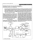

![20 [7] Don Libes, “Using expect to Automate Systems Administration](http://vs1.manualzilla.com/store/data/005773716_1-68a79e060d9ea16881001f4ab808f924-150x150.png)