Download Manual - LibBi

LibBi
User Guide
User Reference
Developer Guide
Version 1.2.0
Developers :
Contributors :
Copyright :
Lawrence Murray
Pierre Jacob
Anthony Lee
Josh Milthorpe
c 2013–2014 CSIRO. This document is distributed under the same terms as the
LibBi software; see the LICENSE file therein.
i
1
User Guide
1
1.1
Introduction . . . . . . . . . . . . . . . . . . . . . . . . . . .
1
1.2
Getting started . . . . . . . . . . . . . . . . . . . . . . . . . .
3
1.3
Models . . . . . . . . . . . . . . . . . . . . . . . . . . . . . .
4
1.3.1
Constants . . . . . . . . . . . . . . . . . . . . . . . .
4
1.3.2
Inlines . . . . . . . . . . . . . . . . . . . . . . . . . .
4
1.3.3
Dimensions . . . . . . . . . . . . . . . . . . . . . . .
5
1.3.4
Variables . . . . . . . . . . . . . . . . . . . . . . . . .
5
1.3.5
Actions . . . . . . . . . . . . . . . . . . . . . . . . . .
6
1.3.6
Blocks . . . . . . . . . . . . . . . . . . . . . . . . . .
7
1.3.7
Expressions . . . . . . . . . . . . . . . . . . . . . . .
8
1.3.8
Built-in variables . . . . . . . . . . . . . . . . . . . .
9
1.4
Command-line interface . . . . . . . . . . . . . . . . . . . .
9
1.5
Output files . . . . . . . . . . . . . . . . . . . . . . . . . . . 10
1.6
Simulation schema . . . . . . . . . . . . . . . . . . . 10
1.5.2
Particle filter schema . . . . . . . . . . . . . . . . . . 11
1.5.3
Simulation “flexi” schema . . . . . . . . . . . . . . . 11
1.5.4
Particle filter “flexi” schema . . . . . . . . . . . . . . 12
1.5.5
Kalman filter schema . . . . . . . . . . . . . . . . . . 12
1.5.6
Optimisation schema . . . . . . . . . . . . . . . . . . 12
1.5.7
PMCMC schema . . . . . . . . . . . . . . . . . . . . 12
1.5.8
SMC2 schema . . . . . . . . . . . . . . . . . . . . . . 13
Input files . . . . . . . . . . . . . . . . . . . . . . . . . . . . 13
1.6.1
Time variables . . . . . . . . . . . . . . . . . . . . . . 14
1.6.2
Coordinate variables . . . . . . . . . . . . . . . . . . 16
1.6.3
Sampling models with input . . . . . . . . . . . . . 17
1.7
Getting it all working . . . . . . . . . . . . . . . . . . . . . . 18
1.8
Performance guide . . . . . . . . . . . . . . . . . . . . . . . 20
1.9
2
1.5.1
1.8.1
Precomputing . . . . . . . . . . . . . . . . . . . . . . 20
1.8.2
I/O . . . . . . . . . . . . . . . . . . . . . . . . . . . . 21
1.8.3
Configuration . . . . . . . . . . . . . . . . . . . . . . 21
Style guide . . . . . . . . . . . . . . . . . . . . . . . . . . . . 22
User Reference
2.1
23
Models . . . . . . . . . . . . . . . . . . . . . . . . . . . . . . 23
2.1.1
model . . . . . . . . . . . . . . . . . . . . . . . . . . . 23
2.1.2
dim . . . . . . . . . . . . . . . . . . . . . . . . . . . . 23
2.1.3
input, noise, obs, param and state . . . . . . . . . 24
ii
2.2
2.1.4
const . . . . . . . . . . . . . . . . . . . . . . . . . . . 25
2.1.5
inline . . . . . . . . . . . . . . . . . . . . . . . . . . 25
Actions . . . . . . . . . . . . . . . . . . . . . . . . . . . . . . 25
2.2.1
beta . . . . . . . . . . . . . . . . . . . . . . . . . . . 25
2.2.2
cholesky . . . . . . . . . . . . . . . . . . . . . . . . . 26
2.2.3
exclusive_scan . . . . . . . . . . . . . . . . . . . . 26
2.2.4
gamma . . . . . . . . . . . . . . . . . . . . . . . . . . . 26
2.2.5
gaussian . . . . . . . . . . . . . . . . . . . . . . . . . 27
2.2.6
inclusive_scan . . . . . . . . . . . . . . . . . . . . 27
2.2.7
inverse_gamma . . . . . . . . . . . . . . . . . . . . . 28
2.2.8
log_gaussian . . . . . . . . . . . . . . . . . . . . . . 28
2.2.9
log_normal . . . . . . . . . . . . . . . . . . . . . . . 28
2.2.10 normal . . . . . . . . . . . . . . . . . . . . . . . . . . 28
2.2.11 pdf . . . . . . . . . . . . . . . . . . . . . . . . . . . . 29
2.2.12 transpose . . . . . . . . . . . . . . . . . . . . . . . . 29
2.2.13 truncated_gaussian . . . . . . . . . . . . . . . . . . 29
2.2.14 truncated_normal . . . . . . . . . . . . . . . . . . . 30
2.2.15 uniform . . . . . . . . . . . . . . . . . . . . . . . . . 30
2.2.16 wiener . . . . . . . . . . . . . . . . . . . . . . . . . . 31
2.3
Blocks . . . . . . . . . . . . . . . . . . . . . . . . . . . . . . . 31
2.3.1
bridge . . . . . . . . . . . . . . . . . . . . . . . . . . 31
2.3.2
initial . . . . . . . . . . . . . . . . . . . . . . . . . 31
2.3.3
lookahead_observation . . . . . . . . . . . . . . . 31
2.3.4
lookahead_transition . . . . . . . . . . . . . . . . 32
2.3.5
observation . . . . . . . . . . . . . . . . . . . . . . 32
2.3.6
ode . . . . . . . . . . . . . . . . . . . . . . . . . . . . 32
2.3.7
parameter . . . . . . . . . . . . . . . . . . . . . . . . 33
2.3.8
proposal_initial . . . . . . . . . . . . . . . . . . . 33
2.3.9
parameter . . . . . . . . . . . . . . . . . . . . . . . . 34
2.3.10 transition . . . . . . . . . . . . . . . . . . . . . . . 34
2.4
Commands . . . . . . . . . . . . . . . . . . . . . . . . . . . . 34
2.4.1
Build options . . . . . . . . . . . . . . . . . . . . . . 34
2.4.2
Run options . . . . . . . . . . . . . . . . . . . . . . . 36
2.4.3
Common options . . . . . . . . . . . . . . . . . . . . 36
2.4.4
draw . . . . . . . . . . . . . . . . . . . . . . . . . . . 37
2.4.5
filter . . . . . . . . . . . . . . . . . . . . . . . . . . 38
2.4.6
help . . . . . . . . . . . . . . . . . . . . . . . . . . . 40
iii
2.4.7
optimise . . . . . . . . . . . . . . . . . . . . . . . . . 40
2.4.8
optimize . . . . . . . . . . . . . . . . . . . . . . . . . 41
2.4.9
package . . . . . . . . . . . . . . . . . . . . . . . . . 41
2.4.10 rewrite . . . . . . . . . . . . . . . . . . . . . . . . . 43
2.4.11 sample . . . . . . . . . . . . . . . . . . . . . . . . . . 44
3
Developer Guide
46
3.1
Introduction . . . . . . . . . . . . . . . . . . . . . . . . . . . 46
3.2
Setting up a development environment . . . . . . . . . . . 46
3.2.1
Obtaining the source code . . . . . . . . . . . . . . . 46
3.2.2
Using Eclipse . . . . . . . . . . . . . . . . . . . . . . 47
3.3
Building documentation . . . . . . . . . . . . . . . . . . . . 47
3.4
Building releases . . . . . . . . . . . . . . . . . . . . . . . . 48
3.5
Developing the code generator . . . . . . . . . . . . . . . . 48
3.6
3.5.1
Actions and blocks . . . . . . . . . . . . . . . . . . . 48
3.5.2
Clients . . . . . . . . . . . . . . . . . . . . . . . . . . 49
3.5.3
Designing an extension . . . . . . . . . . . . . . . . 50
3.5.4
Documenting an extension . . . . . . . . . . . . . . 50
3.5.5
Developing the language . . . . . . . . . . . . . . . 50
3.5.6
Style guide . . . . . . . . . . . . . . . . . . . . . . . . 50
Developing the library . . . . . . . . . . . . . . . . . . . . . 51
3.6.1
Header files . . . . . . . . . . . . . . . . . . . . . . . 51
3.6.2
Pseudorandom reproducibility . . . . . . . . . . . . 51
3.6.3
Shallow copy, deep assignment . . . . . . . . . . . . 52
3.6.4
Coding conventions . . . . . . . . . . . . . . . . . . 52
3.6.5
Style guide . . . . . . . . . . . . . . . . . . . . . . . . 53
iv
1
User Guide
1.1
Introduction
LibBi is used for Bayesian inference over state-space models, including
simulation, filtering and smoothing for state estimation, and optimisation
and sampling for parameter estimation.
LibBi supports state-space models of the form:


T
p(y1:T , x0:T , θ) =
{z
}
|
joint

T



p(θ) p(x0 |θ) 
p(xt |xt−1 , θ)  ∏ p(yt |xt , θ) .
|{z} | {z } t∏
|
{z
}
{z
}
|
=1
t =1
parameter
|
transition
initial
{z
prior
observation
}|
{z
likelihood
}
(1.1)
where t = 1, . . . , T indexes time, y1:T are observations, x1:T are state
variables, and θ are parameters.
The state-space model in (1.1) consists of four conditional probability
densities:
• the parameter model, specifying the prior density over parameters,
• the initial value model, specifying the prior density over the initial
value of state variables, conditioned on the parameters,
• the transition model, specifying the transition density, conditioned
on the parameters and previous state,
• the observation model, specifying the observation density, conditioned on the parameters and current state.
→ See Models
Each of these is explicitly specified using the LibBi modelling language.
A brief example will help to set the scene. Consider the following LotkaVolterra-like predator-prey model between zooplankton (predator, Z)
and phytoplankton (prey, P):
dP
dt
dZ
dt
= αt P − cPZ
= ecPZ − ml Z − mq Z2 .
Here, t is time (in days), with prescribed constants c = .25, e = .3, ml = .1
and mq = .1. The stochastic growth term, αt , is updated in discrete time
by drawing αt ∼ N (µ, σ ) daily. Parameters to be estimated are µ and σ,
and P is observed, with noise, at daily intervals.
The model above might be specified in the LibBi modelling language as
follows:
/**
* Lotka-Volterra-like phytoplankton-zooplankton (PZ) model.
*/
model PZ {
const c = 0.25
// zooplankton clearance rate
const e = 0.3
// zooplankton growth efficiency
const m_l = 0.1 // zooplankton linear mortality
const m_q = 0.1 // zooplankton quadratic mortality
param mu, sigma
state P, Z
noise alpha
obs P_obs
//
//
//
//
mean and std. dev. of phytoplankton growth
phytoplankton, zooplankton
stochastic phytoplankton growth rate
observations of phytoplankton
sub parameter {
mu ~ uniform(0.0, 1.0)
sigma ~ uniform(0.0, 0.5)
}
sub initial {
P ~ log_normal(log(2.0), 0.2)
Z ~ log_normal(log(2.0), 0.1)
}
sub transition {
alpha ~ normal(mu, sigma)
ode {
dP/dt = alpha*P - c*P*Z
dZ/dt = e*c*P*Z - m_l*Z - m_q*Z*Z
}
}
sub observation {
P_obs ~ log_normal(log(P), 0.2)
}
}
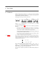
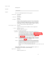
This would be saved in a file named PZ.bi. Various tasks can now be
performed with the LibBi command-line interface, the simplest of which
is just sampling from the prior distribution of the model:
libbi sample --target prior \
--model-file PZ.bi \
--nsamples 128 \
--end-time 365 \
--noutputs 365 \
--output-file results/prior.nc
This command will sample 128 trajectories of the model (--nsamples
128), each of 365 days (--end-time 365), outputting the results every
day (--noutputs 365) to the NetCDF file results/prior.nc.
Tip →
On the first occasion that a command is run, LibBi generates and compiles
code for you behind the scenes. This takes some time, depending on the
complexity of the model. The second time the command is run there is no
such overhead, and execution time is noticeably shorter. Changes to some
command-line options may also trigger a recompile.
To play with this example further, download the PZ package from www.
2
libbi.org. Inspect and run the run.sh script to get started.
The command-line interface provides numerous other functionality, including filtering and smoothing the model with respect to data, and
optimising or sampling its parameters. The help command is particularly useful, and can be used to access the contents of the User Reference
portion of this manual from the command line.
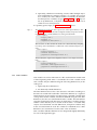
1.2
Getting started
There is a standard file and directory structure for a LibBi project. Using
it for your own projects ensures that they will be easy to share and
distribute as a LibBi package. To set up the standard structure, create an
empty directory somewhere, and from within that directory run:
libbi package --create --name Name
replacing Name with the name of your project.
Tip →
By convention, names always begin with an uppercase letter, and all new
words also begin with an uppercase letter, as in CamelCase. See the Style
guide for more such conventions.
Each of the files that are created contains some placeholder content that
is intended to be modified. The META.yml file can be completed immediately with the name of the package, the name of its author and a brief
description. This and other files are detailed with the package command.
This early stage is also the ideal time to think about version control. LibBi
developers use Git for version control, and you may like to do the same
for your project. A new repository can be initialised in the same directory
with:
git init
Then add all of the initial files to the repository and make the first commit:
git add *
git commit -m ’Added initial files’
The state of the repository at each commit may be restored at any stage,
allowing old versions of files to be maintained without polluting the
working directory.
A complete introduction to Git is beyond the scope of this document.
See www.git-scm.com for more information. The documentation for the
package command also gives some advice on what to include, and what
not to include, in a version control repository.
The following command can be run at any time to validate that a project
still conforms to the standard structure:
libbi package --validate
Finally, the following command can be used to build a package for distribution:
3
libbi package --build
This creates a *.tar.gz file in the current directory containing the project
files.
1.3
Models
Models are specified in the LibBi modelling language. A model specification is put in a file with an extension of *.bi. Each such file contains
only a single model specification.
A specification always starts with an outer model statement that declares
and names the model. It then proceeds with declarations of constants,
dimensions and variables, followed by four top-level blocks – parameter,
initial, transition and observation – that describe the factors of the
state-space model.
A suitable template is:
model Name {
// declare constants...
// declare dimensions...
// declare variables...
sub parameter {
// specify the parameter model...
}
sub initial {
// specify the initial condition model...
}
sub transition {
// specify the transition model...
}
sub observation {
// specify the observation model...
}
}
Note that the contents of the model statement and each top-level block are
contained in curly braces ({. . .}), in typical C-style. Comments are also
C-style, an inline comment being wrapped by /* and */, and the doubleslash (//) denoting an end-of-line comment. Lines may optionally end
with a semicolon.
1.3.1
Constants
→ See also const
Constants are named and immutable scalar values. They are declared
using:
const name = constant_expression
Often constant_expression is simply a literal value, but in general it
may be any constant scalar expression (see Expressions).
1.3.2
Inlines
→ See also inline
Inlines are named scalar expressions. They are declared using:
4
inline name = expression
Any use of the inline name in subsequent expressions is precisely equivalent to wrapping expression in parentheses and replacing name with it.
Inlines may be recursively nested.
1.3.3
Dimensions
Dimensions are used to construct vector, matrix and higher-dimensional
variables. Often, but not necessarily, they have a spatial interpretation;
for example a large 3-dimensional spatial model may declare dimensions
x, y and z. Dimensions are declared using:
→ See also dim
dim name (size )
Tip →
1.3.4
Because LibBi is primarily meant for state-space models, the time dimension
is special and not declared explicitly. Consider that, for continuous-time
models, time is not readily represented by a dimension of a finite size.
Variables
→ See also input, param, state,
noise and obs
Variables are named and mutable scalar, vector, matrix or higher-dimensional
objects.
A simple scalar variable is declared using:
type name
where type is one of:
input :
for a variable with values that may or may not change over time,
but that are prescribed according to input from a file,
param :
for a latent variable that does not change over time,
state :
for a latent variable that changes over time,
noise :
for a latent noise term that changes over time,
obs :
for an observed variable that changes over time.
For example, for the equation of the state-space model in the Introduction,
the parameter θ may be declared using:
param theta
the state variable x using:
state x
and the observed variable y using:
obs y
A vector, matrix or higher-dimensional variable is declared by listing the
names of the Dimensions over which it extends, separated by commas,
in square brackets after the variable name. For example:
5
dim m(50)
dim n(20)
...
state x[m,n]
declares a state variable x, which is a matrix of size 50 × 20.
The declaration of a variable can also include various arguments that
control, for example, whether or not it is included in output files. These
are specified in parentheses after the variable declaration, for example:
state x[m,n](has_output = 0)
1.3.5
Actions
Within each top-level block, a probability density is specified using actions.
Simple actions take one of three forms:
x ~ expression
x <- expression
dx/dt = expression
where x is some variable, referred to as the target. Named actions, available only for the first two forms, look like:
x ~ name (arguments , ...)
x <- name (arguments , ...)
The first form, with the ˜ operator, indicates that the (random) variable x
is distributed according to the action given on the right. Such actions are
usually named, and correspond to parametric probability distributions
(e.g. gaussian, gamma and uniform). If the action is not named, the
expression on the right is assumed to be a probability density function.
The second form, with the <- operator, indicates that the (conditionally deterministic) variable x should be assigned the result of the action
given on the right. Such actions might be simple scalar, vector or matrix
expressions.
The third form, with the = operator, is for expressing ordinary differential
equations.
Individual elements of a vector, matrix or higher-dimensional variable
may be targeted using square brackets. Consider the following action
giving the ordinary differential equation for a Lorenz ’96 model:
dx[i]/dt = x[i - 1]*(x[i + 1] - x[i - 2]) - x[i] + F
If x is a vector of size N, the action should be interpreted as “for each
i ∈ {0, . . . , N − 1}, use the following ordinary differential equation”. The
name i is an index, considered declared on the left with local scope to
the action, so that it may be used on the right. The name i is arbitrary,
but must not match the name of a constant, inline or variable. It may
match the name of a dimension, and indeed matching the name of the
dimension with which the index is associated can be sensible.
Elements of higher-dimensional variables may be targeted using multiple indices separated by commas. For example, consider computing a
Euclidean distance matrix D:
6
D[i,j] <- sqrt(pow(x[i] - x[j], 2) - pow(y[i] - y[j], 2))
If D is a matrix of size M × N, the action should be interpreted as “for
each i ∈ {0, . . . , M − 1} and each j ∈ {0, . . . , N − 1} . . .”.
Indices may be restricted with a range:
D[i=0:3,j=2:3] <- sqrt(pow(x[i] - x[j], 2) - pow(y[i] - y[j], 2))
Now action should be interpreted as “for each i ∈ {0, . . . , 3} and each
j ∈ {2, 3} . . .”.
Indexed actions such as this are useful for more complicated transformations that either cannot be expressed in matrix form, or that are contrived
when expressed as such.
Arguments to actions may be given with either positional or named forms,
or a mix of the two. Positional arguments are interpreted by the order
given. For example
x ~ gaussian(0.0, 2.0)
means that x is distributed according to the gaussian action with, by
the definition of that action, mean 0.0 and standard deviation 2.0. The
gaussian action also happens to support named arguments, so the following is equivalent:
x ~ gaussian(mean = 0.0, std = 2.0)
The order of named arguments is unimportant, so the following is also
equivalent:
x ~ gaussian(std = 2.0, mean = 0.0)
Positional and named arguments may be mixed, but all positional arguments must appear before all named arguments. Thus, this is valid:
x ~ gaussian(0.0, std = 2.0)
but these are not:
x ~ gaussian(mean = 0.0, 2.0)
x ~ gaussian(std = 2.0, 0.0)
This avoids ambiguity in the syntax.
The documentation for an action lists its arguments, and whether it may
be used in named or positional form, or both.
1.3.6
Blocks
Some actions are more complicated and can, or must, be wrapped in
blocks. Good examples are systems of ordinary differential equations.
Two or more equations must be grouped to form the complete system.
The grouping is achieved with the ode block.
Consider the following Lotka-Volterra-type transition model:
7
sub transition {
sub ode {
dP/dt = alpha*P - c*P*Z
dZ/dt = e*c*P*Z - m_l*Z
}
}
Here, the ode block combines the two actions into the one system of
ordinary differential equations.
Like actions, blocks can take arguments. The ode block has parameters to
select and configure the algorithm used to numerically integrate the differential equations forward through time. If the defaults are inadequate,
these might be set as follows:
sub transition {
sub ode(atoler = 1.0e-3, rtoler = 1.0e-3, alg = ’dopri5’) {
dP/dt = alpha*P - c*P*Z
dZ/dt = e*c*P*Z - m_l*Z
}
}
As for actions, both positional and named forms of arguments are supported.
1.3.7
Expressions
LibBi supports expressions over scalars, vectors, matrices and higherdimensional variables:
• A scalar is a literal, constant or variable that is not declared over
any dimensions.
• A vector is a variable declared over exactly one dimension.
• A matrix is a variable declared over exactly two dimensions.
• Variables declared over three or more dimensions are not given a
special name.
Note that, by these definitions, a variable declared over a single dimension of size one is considered a vector, not a scalar. Any variable declared
over more than one dimension, where all of those dimensions have size
one, is likewise not considered a scalar. The reason for this is that the
particular boundary conditions of those dimensions may convey different
behaviour to that of a scalar.
Special classes of expression are:
• A constant expression is one that can be evaluated at compile time. It
must be scalar, and may refer to literals, constants and inlines that
expand to other constant expressions only.
• A static expression is one that does not depend on time. It may
refer to literals, constants, variables of type param, and inlines that
expand to other static expressions only.
• A common expression is one that does not depend on the state of a
particular trajectory. It may refer to literals, constants, variables
of type param or input, and inlines that expand to other common
expressions only.
8
Note from these definitions that a constant expression is a static expression, and a static expression is a common expression.
Individual elements of multidimensional variables may be indexed with
e.g. x[i] or A[i,j]. Ranges may also be referenced by giving the first and
last indices of the range, separated by a colon, e.g. x[0:3] or A[0:3,2:3].
The following operators are supported in expressions:
Scalar/vector/matrix arithmetic operators:
Element-wise vector/matrix operators:
Comparison operators:
Logical operators:
Ternary operators:
+ - * / % **
.+ .- .* ./ .% .**
== != < <= > >=
&& ||
?:
The following functions are supported in expressions:
abs acos acosh asin asinh atan atan2 atanh ceil cos cosh erf
erfc exp floor gamma lgamma log max min mod pow round sin
sinh sqrt tan tanh
1.3.8
Built-in variables
The following built-in variables are supported:
t_now
t_last_input
t_next_obs
1.4
the current time,
the last time at which an input variable was updated,
the next time at which an obs variable will be updated.
Command-line interface
Methods are applied to models via the command-line interface of LibBi.
This is invoked using:
libbi command options ...
where command is any one of the following:
filter :
for filtering problems using the model and observations,
optimise :
for parameter optimisation problems using the model and observations,
sample :
for parameter and state sampling problems using the model and
observations,
package :
for creating projects and building packages for distribution,
help :
for accessing online help,
draw :
to visualise a model (useful for debugging and development),
rewrite :
to inspect the internal representation of a model (useful for debugging and development),
and available options depend on the command.
Options may be specified in a configuration file or on the command
line itself. To use a configuration file, give the name of the file on the
command line, preceded by @, e.g.
9
libbi command @command.conf
More than one config file may be specified, each preceded by @. An
option given on the command line will override an option of the same
name given in the configuration file.
A config file simply contains a list of command-line options just as they
would be given on the command line itself. For readability, the commandline options may be spread over any number of lines, and end-of-line
comments, preceded by #, may appear. The contents of one config file
may be nested in another by using the @file.conf syntax within a file.
This can be useful to avoid redundancy. For example, the sample command inherits all the options of filter. In this case it may be useful to
write a filter.conf file that is nested within a sample.conf file, so that
options need not be repeated.
1.5
Output files
LibBi uses NetCDF files for input and output. A NetCDF file consists
of dimensions, along with variables extending across them. This is very
similar to LibBi models. Where use of these overloaded names may cause
confusion, the specific names NetCDF variable/dimension and model variable/dimension are used throughout this section and the next. A NetCDF
file may also contain scalar attributes that provide meta information.
The schema of a NetCDF file is its structure with respect to the dimensions,
variables and attributes that it contains. Among the dimensions will be
those that correspond to model dimensions. Likewise for variables. Some
additional dimensions and variables will provide critical method-specific
information or diagnostics.
Tip →
To quickly inspect the structure and contents of a NetCDF file, use the
ncdump utility, included as standard in NetCDF distributions:
ncdump file.nc | less
LibBi output files have several schemas. The schema of an output file
depends on the command that produces it, and the options given to that
command. The schemas are related by strong conventions and inherited
structure.
This section outlines each schema in turn. The syntax x[m,n] is used
to refer to a NetCDF variable named x that extends across the NetCDF
dimensions named m and n.
Tip →
1.5.1
If using OctBi or RBi for collating and visualising the output of LibBi, it may
be unnecessary to understand these schema, as they are encapsulated by
the higher-level functions of these packages.
Simulation schema
This schema is used by the sample command when the target option is
set to prior, joint or prediction. It consists of dimensions:
• nr indexing time,
10
• np indexing trajectories, and
• for each dimension n in the model, a dimension n .
And variables:
• time[nr] giving the output times,
• for each param variable theta in the model, defined over dimensions m,...,n , a variable theta [m,...,n ], and
• for each state and noise variable x in the model, defined over
dimensions m,...,n , a variable x [nr,m,...,n,np].
1.5.2
Particle filter schema
This schema is used by the filter command when a particle filter, besides the adaptive particle filter, is chosen. It extends the simulation
schema, with the following changes:
• the np dimension is now interpreted as indexing particles not trajectories.
The following variables are added:
• logweight[nr,np] giving the log-weights vector at each time, and
• ancestor[nr,np] giving the ancestry vector at each time.
Tip →
1.5.3
To draw a whole trajectory out of a file of the particle filter schema, begin at
the last time, select a particle, and use the ancestor vector at each time to
trace that particle’s ancestry back through time. One cannot simply take a
row from the matrix of a state variable to obtain a complete trajectory, as
with the simulation schema.
Simulation “flexi” schema
This schema is currently not used directly, but the particle filter “flexi”
schema below extends it. The complication here is that the number of
particles at each time can vary. The schema consists of the following
dimensions:
• nr indexing time,
• nrp indexing both time and trajectories (an unlimited dimension),
and
• for each dimension n in the model, a dimension n .
And variables:
• time[nr] giving the output times,
• start[nr] giving, for each time, the starting index along the nrp
dimension for particles associated with that time,
• len[nr] giving, for each time, the number of particles at that time,
• for each param variable theta in the model, defined over dimensions m,...,n , a variable theta [m,...,n ], and
• for each state and noise variable x in the model, defined over
dimensions m,...,n , a variable x [m,...,n,nrp].
11
Tip →
1.5.4
With the “flexi” schema, to read the contents of a variable at some time
index t , read len[t ] entries along the nrp dimension, beginning at index
start[t ].
Particle filter “flexi” schema
This schema is used by the filter command when an adaptive particle
filter is chosen. It extends the simulation “flexi” schema. The following
variables are added:
• logweight[nrp] giving the log-weights vector at each time, and
• ancestor[nrp] giving the ancestry vector at each time.
1.5.5
Kalman filter schema
This schema is used by the filter command when a Kalman filter is
chosen. It extends the simulation schema, with the following changes:
• the np dimension is always of size 1, and
• variables that correspond to state and noise variables in the model
are now interpreted as containing the mean of the filter density at
each time.
The following dimensions are added:
• nxcol indexing columns of matrices, and
• nxrow indexing rows of matrices.
The following variables are added:
• U_[nr,nxcol,nxrow] containing the upper-triangular Cholesky
factor of the covariance matrix of the filter density at each time.
• For each noise and state variable x , a variable index.x giving the
index of the first row (and column) in S_ pertaining to this variable,
the first such index being zero.
1.5.6
Optimisation schema
This schema is used by the optimise command. It consists of dimensions:
• np indexing iterations of the optimiser (an unlimited dimension).
And variables:
• for each param variable theta in the model, defined over dimensions m,...,n , a variable theta [m,...,n,np],
• optimiser.value[np] giving the value of the function being optimised at each iteration, and
• optimiser.size[np] giving the value of the convergence criterion
at each iteration.
1.5.7
PMCMC schema
This schema is used by the sample command when a PMCMC method is
chosen. It extends the simulation schema, with the following changes:
• the np dimension indexes samples, not trajectories, and
12
• for each param variable theta in the model, defined over dimensions m,...,n , there is a variable theta [m,...,n,np] instead of
theta [m,...,n ] (i.e. param variables are defined over the np dimension also).
The following variables are added:
• loglikelihood[np] giving the log-likelihood estimate p̂(y1:T |θp )
for each sample θp , and
• logprior[np] giving the log-prior density p(θp ) of each sample
θp .
1.5.8
SMC2 schema
This schema is used by the sample command when an SMC2 method is
chosen. It extends the PMCMC schema, with the following additional
variables:
• logweight[np] giving the log-weights vector of parameter samples.
• logevidence[nr] giving the incremental log-evidence of the model
at each time.
1.6
Input files
Input files take three forms:
• initialisation files, containing the initial values of state variables,
• input files, containing the values of input variables, possibly changing across time, and
• observation files, containing the observed values of obs variables.
All of these use the same schema. That schema is quite flexible, allowing
for the representation of both dense and sparse input. Sparsity may be
in time or space. Sparsity in time is, for example, having a discrete-time
model with a scalar obs variable that is not necessary observed at all
times. Sparsity in space is, for example, having a discrete-time model
with a vector obs variable, for which not all of the elements are necessarily
observed at all times.
Each model variable is associated with a NetCDF variable of the same
name. Additional NetCDF variables may exist. Model variables which
cannot be matched to a NetCDF variable of the same name do not receive
input from the file. For input variables, this means that they will remain
uninitialised. For spatially dense input, each such NetCDF variable may
be defined along the following dimensions, in the order given:
1. Optionally, a dimension named ns, used to index multiple experiments set up in the same file. If not given for a variable, that
variable is assumed to be the same for all experiments.
2. Optionally, a time dimension (see below).
3. Optionally, a number of dimensions with names that match the
model dimensions along which the model variable is defined, ordered accordingly,
13
4. Optionally, a dimension named np, used to index multiple trajectories (instantiations, samples, particles) of a variable. If not given
for a variable, the value of that variable is assumed to be the same
for all trajectories. Variables of type param, input and obs may not
use an np dimension, as by their nature they are meant to be in
common across all trajectories.
For spatially sparse input, see Coordinate variables below.
Tip →
1.6.1
The Simulation schema is in fact a special case of the input schema, so that
the sample command can often be used quite sensibly as input to another
run. For example, a simulated data set can be generated with:
libbi sample \
--target joint \
--nsamples 1 \
--output-file data/obs.nc \
...
The data/obs.nc file can then be used as an observation file, sampling
from the posterior distribution conditioned on the simulated trajectory as
data:
libbi sample \
--target posterior \
--obs-file data/obs.nc \
--output-file results/posterior.nc \
...
Then, indeed, the output of that might be fed into a new sample forward in
time:
libbi sample \
--target prediction \
--init-file results/posterior.nc \
--output-file results/prediction.nc \
....
Time variables
Time variables are used to index time in a file. Each NetCDF variable with
a name beginning with “time” is assumed to be a time variable. Each
such variable may be defined along the following dimensions, in the
order given:
1. Optionally, the ns dimension.
2. An arbitrarily named dimension.
The latter dimension becomes a time dimension. The time variable gives
the time associated with each index of that time dimension, a sequence
which must be monotonically non-decreasing. NetCDF variables that
correspond to model variables, and that are defined along the same time
dimension, become associated with the time variable. The time dimension thus enumerates both the times at which these variables change,
and the values that they are to assume at those times. A variable may
only be associated with one time dimension, and param variables may
not be associated with one at all. If a variable is not defined across a time
dimension, it is assumed to have the same value at all times.
Time variables and time dimensions are interpreted slightly differently
for each of the input file types:
14
1. For an initialisation file, the starting time (given by the --start-time
command-line option, see filter) is looked-up in each time variable, and the corresponding record in each associated variable is
used for its initialisation.
2. For input files, a time variable gives the times at which each associated variable changes in value. Each variable maintains its new
value until the time of the next change.
3. For observation files, a time variable gives the times at which each
associated variable is observed. The value of each variable is interpreted as being its value at that precise instant in time.
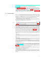
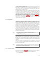
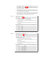
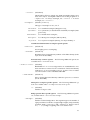
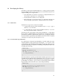
Example →
Representing a scalar input
Assume that we have an obs variable named y, and we wish to construct an
observation file containing our data set, which consists of observations of y
at various times. A valid NetCDF schema would be:
• a dimension named nr, to be our time dimension,
• a variable named time_y, defined along the dimension nr, to be our
time variable, and
• a variable named y, defined along the dimension nr, to contain the
observations.
We would then fill the variable time_y with the observation times of our
data set, and y with the actual observations. It may look something like this:
time_y[nr]
y[nr]
0.0
6.75
1.0
4.56
2.0
9.45
5.5
4.23
6.0
7.12
9.5
5.23
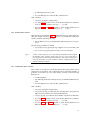
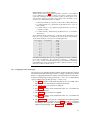
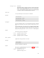
Example →
Representing a vector input, densely
Assume that we have an obs variable named y, which is a vector defined
across a dimension of size three called n. We wish to construct an observation file containing a our data set, which consists of observations of y at
various times, where at each time all three elements of y are observed. A
valid NetCDF schema would be:
• a dimension named nr, to be our time dimension,
• a variable named time_y, defined along the dimension nr, to be our
time variable,
• a dimension named n, and
• a variable named y, defined along the dimensions nr and n, to contain
the observations.
We would then fill the variable time_y with the observation times of our
data set, and y with the actual observations. It may look something like this:
time_y[nr]
y[nr,n]
0.0
6.75 3.34 3.45
1.0
4.56 4.54 1.34
2.0
9.45 3.43 1.65
5.5
4.23 8.65 4.64
6.0
7.12 4.56 3.53
9.5
5.23 3.45 3.24
15
1.6.2
Coordinate variables
Coordinate variables are used for spatially sparse input. Each variable with
a name beginning with “coord” is assumed to be a coordinate variable.
Each such variable may be defined along the following dimensions, in
the order given:
1. Optionally, the ns dimension.
2. A coordinate dimension (see below).
3. Optionally, some arbitrary dimension.
The second dimension, the coordinate dimension, may be a time dimension
as well. NetCDF variables that correspond to model variables, and that
are defined along the same coordinate dimension, become associated
with the coordinate variable. The coordinate variable is used to indicate
which elements of these variables are active. The last dimension, if
any, should have a length equal to the number of dimensions across
which these variables are defined. So, for example, if these variables are
matrices, the last dimension should have a length of two. If the variables
are vectors, so that they have only one dimension, the coordinate variable
need not have this last dimension.
If a variable specified across one or more dimensions in the model cannot be associated with a coordinate variable, then it is assumed to be
represented densely.
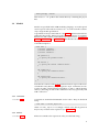
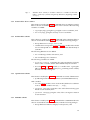
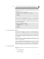
Example →
16
Representing a vector input, sparsely
Assume that we have an obs variable named y, which is a vector defined
across a dimension of size three called n. We wish to construct an observation file containing our data set, which consists of observations of y at
various times, where at each time only a subset of the elements of y are
observed. A valid NetCDF schema would be:
• a dimension named nr, to be both our time and coordinate dimension,
• a variable named time_y, defined along the dimension nr, to be our
time variable,
• a variable named coord_y, defined along the dimension nr, to be our
coordinate variable,
• a variable named y, defined along the dimension nr, to contain the
observations.
We would then fill the variable time_y with the observation times of our
data set, coord_y with the coordinate of each observation, and y with the
observations themselves. It may look something like this:
time_y[nr]
coord_y[nr]
y[nr]
0.0
0
6.75
0.0
1
3.34
1.0
0
4.56
1.0
1
4.54
1.0
2
1.34
2.0
1
3.43
5.5
3
4.64
6.0
0
4.23
6.0
2
3.53
9.5
1
3.45
Note that each unique value in time_y is repeated for as many coordinates
as are active at that time. Also note that, if y had m > 1 dimensions,
the coord_y variable would be defined along some additional, arbitrarily
named dimension of size m in the NetCDF file, so that the values of coord_y
in the above table would be vectors.
1.6.3
Sampling models with input
The precise way in which input files and the model specification interact
is best demonstrated in the steps taken to sample a model’s prior distribution. Computing densities is similar. The initialisation file referred to
in the proceeding steps is that given by the --init-file command-line
option, and the input file that given by --input-file.
1. Any input variables in the input file that are not associated with a
time variable are initialised by reading from the file.
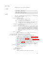
2. The parameter top-level block is sampled.
3. Any param variables in the initialisation file are overwritten by
reading from the file.
4. The initial top-level block is sampled.
5. Any state variables in the initialisation file are overwritten by
reading from the file.
6. The transition top-level block is sampled forward through time.
Sampling stops at each time that an input variable is to change,
according to the input file, at which point the input variable is
updated and sampling of the transition block continues.
17
Note two important points in this procedure:
• An input variable in the input file that is not associated with a
time variable is initialised before anything else, whereas an input
variable that is associated with a time variable is not initialised until
simulation begins, even if the first entry of that variable indicates
an update at time zero. This has implications as to which input
variables are, or are not, initialised at the time that the parameter
block is sampled.
• While the parameter and initial blocks are always sampled, the
samples may be later overwritten from the initialisation file. Thus,
the initialisation file need not contain a complete set of variables,
although behaviour is more intuitive if it does. This behaviour also
ensures pseudorandom reproducibility regardless of the presence,
or content, of the initialisation file.
1.7
Getting it all working
This section contains some general advice on the statistical methods employed by LibBi and the tuning that might be required to make the most of
them. It concentrates on the particle marginal Metropolis-Hastings (PMMH)
sampler, used by default by the sample command when sampling from
the posterior distribution.
PMMH is of the family of particle Markov chain Monte Carlo (PMCMC)
methods (Andrieu et al., 2010), which in turn belong to the family of
Markov chain Monte Carlo (MCMC). A complete introduction to PMMH
is beyond the scope of this manual. Murray (2013) provides an introduction of the method and its implementation in LibBi.
When using MCMC methods it is common to perform some short pilot
runs to tune the parameters of the method in order to improve its efficiency, before performing a final run. In PMMH, the parameters to be
tuned are the proposal distribution, and the number of particles in the
particle filter, or sequential Monte Carlo (Doucet et al., 2001), component
of the method.
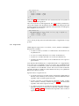
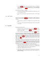
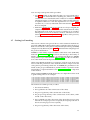
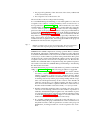
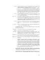
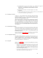
When running PMMH in LibBi, diagnostics are output that can be used
to guide tuning. Here is an example:
22:
23:
24:
25:
26:
-116.129
-116.129
-116.129
-116.129
-116.129
-16.984
-16.984
-16.984
-16.984
-16.984
7.25272
5.63203
6.89478
0.643236
3.58096
beats
beats
beats
beats
beats
-121.853
-119.772
-121.268
-136.661
-128.692
-17.6397
-18.0891
-19.3354
-21.5339
-20.3304
7.49326
6.07209
8.25723
6.44331
6.3502
accept=0.217391
accept=0.208333
accept=0.2
accept=0.192308
accept=0.185185
The numerical columns provide, in order:
1. the iteration number,
2. the log-likelihood of the current state of the chain,
3. the prior log-density of the current state of the chain,
4. the proposal log-density of the current state of the chain, conditioned on the other state,
5. the log-likelihood of the other state of the chain (the previous state
if the most recent proposal was accepted, the last proposed state if
the most recent proposal was rejected),
6. the prior log-density of the other state of the chain,
18
7. the proposal log-density of the other state of the chain, conditioned
on the current state, and
8. the acceptance rate of the chain so far.
The last of these is the most important for tuning.
For a standard Metropolis-Hastings, a reasonable guide is to aim at an
acceptance rate of 0.5 for a single parameter, down to 0.23 for five or
more parameters (Gelman et al., 1994). This includes the case where
a Kalman filter is being used rather than a particle filter (by using the
--filter kalman option to sample). In such cases the only tuning to
perform is that of the proposal distribution. The proposal distribution
is given in the proposal_parameter block of the model specification. If
this block is not specified, the parameter block is used instead, and this
may make for a poor proposal distribution, especially when there are
many observations. Increasing the width of the proposal distribution
will decrease the acceptance rate. Decreasing the width of the proposal
distribution will increase the acceptance rate.
Tip →
Higher acceptance rates are not necessarily better. They may simply be a
result of the chain exploring the posterior distribution very slowly.
PMMH has the added complication of using a particle filter to estimate
the likelihood, rather than a Kalman filter to compute it exactly (although
note that the Kalman filter works only for linear and Gaussian models). It
is necessary to set the number of particles in the particle filter. More particles decreases the variance in the likelihood estimator and so increases the
acceptance rate, but also increases the computational cost. Because the
likelihood is estimated and not computed exactly, the optimal acceptance
rate will be lower than for standard Metropolis-Hastings. Anecdotally,
0.1–0.15 seems reasonable.
The tradeoff between proposal size and number of particles is still under
study, e.g. Doucet et al. (2013). The following procedure is suggested.
1. Start with an empty proposal_parameter block. Set the simulation time (--end-time) to the time of the first observation, and the
number of particles (--nparticles) to a modest amount. When
running PMMH, it is then the case that the same state of the chain,
its starting state in fact, will be proposed repeatedly, and the acceptance rate will depend entirely on the variance of the likelihood
estimator. One hopes to see a high acceptance rate here, say 0.5 or
more. Increase the number of particles until this is achieved. Note
that the random number seed can be fixed (--seed) if you wish.
2. Steadily extend the simulation time to include a few more observations on each attempt, and increase the number of particles as
needed to maintain the high acceptance rate. The number of particles will typically need to scale linearly with the simulation time.
Consult the Performance guide to improve execution times and
further increase the number of particles if necessary.
3. If a suitable configuration is achieved for the full data set, or a
workable subset, the proposal distribution can be considered. You
may find it useful to add one parameter at a time to the proposal
distribution, working towards an overall acceptance rate of 0.1–
0.15.
19
4. If this fails to find a working combination with a healthy acceptance
rate, consider the initialisation of the chain. By default, LibBi simply
draws a sample from the parameter model to initialise the chain. If
this is in an area where the variance in the likelihood estimator is
high, the chain may mix untenably slowly for any sensible number
of particles. It has been observed empirically that the variance in the
likelihood estimator is heteroskedastic, and tends to increase with
distance from the maximum likelihood (Murray et al., 2013). So
initialising the chain closer to the maximum likelihood may allow it
to mix well with a reasonable number of particles. Prior knowledge,
optimisation of parameters (perhaps with the optimise command),
or exploration of the data set may inform the initialisation. The
initialisation can be given in the initialisation file (--init-file).
Tip →
It can also be the case that, in steadily extending the simulation time
(--end-time), the acceptance rate suddenly drops at a particular time. This
indicates that the particle filter degenerates at this point. Improving the
initialisation of the chain is the best strategy in this case, although increasing
the number of particles may help in mild cases.
Be aware that LibBi uses methods that are still being actively developed,
and applied to larger and more complex models. It may be the case that
your model or data set exceeds the current capabilities of the software.
In such cases the only option is to consider a smaller or simpler model,
or a subsample of the available data.
1.8
Performance guide
One of the aims of LibBi is to alleviate the user from performance considerations as much as possible. Nevertheless, there is some scope to
influence performance, particularly by ensuring that appropriate hardware resources are used, and by limiting I/O where possible.
1.8.1
Precomputing
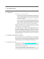
LibBi will:
• precompute constant subexpressions, and
• precompute static subexpressions in the transition and observation
models.
Reducing redundant or repetitious expressions is thus unnecessary where
these are constant or static. For example, taking the square-root of a
variance parameter need not be of concern:
param sigma2
...
sub transition {
epsilon ~ gaussian(mu, sqrt(sigma2))
...
}
Here, sqrt(sigma2) is a static expression that will be extracted and
precomputed outside of the transition block.
Tip →
20
Use the rewrite command to inspect precisely which expressions have
been extracted for precomputation.
1.8.2
I/O
The following I/O options are worth considering to reduce the size of
output files and so the time spent writing to them:
• When declaring a variable, use a has_output = 0 argument to omit
it from output files if it will not be of interest.
• Enable output files by using the --enable-single command-line
option. This will reduce write size by up to a half. Note, however,
that all computations are then performed in single precision too,
which may have significant numerical implications.
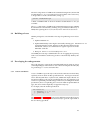
1.8.3
Configuration
The following configuration options are worth considering:
• Internally, LibBi uses extensive assertion checking to catch programming and code generation errors. These assertion checks are
enabled by default, improving robustness at the expense of performance. It is recommended that they remain enabled during model
development and small-scale testing, but that they are disabled
for final production runs. They can be disabled by adding the
--disable-assert command-line option.
• Experiment with the --enable-cuda command-line option to make
use of a CUDA-enabled GPU. This should usually improve performance, as long as a sufficient number of model trajectories are to
be simulated (typically upwards of 1024). If CUDA is being used,
also try the --enable-gpu-cache command-line option if running
PMCMC or SMC2 . This caches particle histories in GPU rather than
main memory. As GPU memory is usually much more limited than
main memory, and this may result in its exhaustion, the option is
disabled by default.
• Experiment with the --enable-sse and --enable-avx commandline options to make use of CPU SSE and AVX SIMD instructions. In
single precision, these can provide up to a four-fold (SSE) or eightfold (AVX) speed-up, and in double precision a two-fold (SSE) or
four-fold (AVX) speed-up. These are only supported on x86 CPU
architectures, however, and AVX in particular only on the most
recent of these.
• Experiment with the --nthreads command-line option to set the
number of CPU threads. Typically there are depreciating gains
as the number of threads is increased, and beyond the number of
physical CPU cores performance will degrade significantly. For
CPUs with hyperthreading enabled, it is recommended that the
number of threads is set to no more than the number of physical
CPU cores. This may be half the default number of threads.
• Experiment with using single precision floating point operations by
using the --enable-single command-line option. This can offer
significant performance improvements (especially when used in
conjunction with the --enable-cuda and --enable-sse options),
21
but care should be taken to ensure that numerical error remains
tolerable. The use of single precision will also reduce memory
consumption by up to a half.
• Use optimised versions of libraries, especially the BLAS and LAPACK libraries.
• Use the Intel C++ compiler if available. Anecdotally, this tends
to produce code that runs faster than gcc. The configure script
should automatically detect the Intel C++ compiler, and use it if
available. To use the Intel Math Kernel Library as well, which is
not automatically detected, use the --enable-mkl command-line
option.
1.9
Style guide
The following conventions are used for LibBi model files:
• Model names are CamelCase, the first letter always capitalised.
• Action and block names are all lowercase, with multiple words
separated by underscores.
• Dimension and variable names should be consistent, where possible, with their counterparts in a description of the model as it might
appear in a scientific paper. For example, single upper-case letters
for the names of matrix variables are appropriate, and standard
symbols (rather than descriptive names) are encouraged. Greek
letters should be written out in full, the first letter capitalised for
the uppercase version (e.g. gamma and Gamma).
• Comments should be used liberally, with descriptions provided
for all dimensions and variables in particular. Consider including
units as part of the description, where relevant.
• Names ending in an underscore are intended for internal use only.
They are not expected to be seen in a model file.
• Indent using two spaces, and do not use tabs.
Finally, use the package command to set up the standard files and directory structure for a LibBi project. This will make your model and its
associated files easy to distribute, and your results easy to reproduce.
22
2
2.1
2.1.1
User Reference
Models
model
Declare a model.
Synopsis
model Name {
...
}
Description
A model statement declares and names a model, and encloses declarations
of the constants, dimensions, variables, inlines and top-level blocks that
specify that model.
The following named top-level blocks are supported, and should usually
be provided:
• parameter, specifying the prior density over parameters,
• initial, specifying the prior density over initial conditions,
• transition, specifying the transition density, and
• observation, specifying the observation density.
The following named top-level blocks are supported, and may optionally
be provided:
• proposal_parameter, specifying a proposal density over parameters,
• proposal_initial, specifying a proposal density over initial conditions,
• lookahead_transition, specifying a lookahead density to accompany the transition density, and
• lookahead_observation, specifying a lookahead density to accompany the observation density.
2.1.2
dim
Declare a dimension.
Synopsis
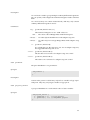
dim name (100, ’cyclic’)
dim name (size = 100, boundary = ’cyclic’)
Description
A dim statement declares a dimension with a given size and boundary
condition.
A dimension may be declared anywhere in a model specification. Its
scope is restricted to the block in which it is declared. A dimension must
be declared before any variables that extend along it are declared.
Arguments
size :
(position 0, mandatory)
Length of the dimension.
boundary :
(position 1, default ’none’)
Boundary condition of the dimension. Valid values are:
’none’ :
2.1.3
No boundary condition.
’cyclic’ :
Cyclic boundary condition; all indexing is taken modulo the
size of the dimension.
’extended’ :
Extended boundary condition; indexes outside the range of the
dimension access the edge elements, as if these are extended
indefinitely.
input, noise, obs, param and state
Declare an input, noise, observed, parameter or state variable.
Synopsis
state
state
state
state
state
state
x
x[i]
X[i,j]
X[i,j,k]
X[i,j](has_output = 0)
x, y, z
//
//
//
//
//
//
scalar variable
vector variable
matrix variable
higher-dimensional variable
omit from output files
multiple variables
Description
Declares a variable of the given type, extending along the dimensions
listed between the square brackets.
A variable may be declared anywhere in a model specification. Its scope
is restricted to the block in which it is declared. Dimensions along which a
variable extends must be declared prior to the declaration of the variable,
using the dim statement.
Arguments
has_input :
(default 1)
Include variable when doing input from a file?
has_output :
(default 1)
Include variable when doing output to a file?
input_name :
(default the same as the name of the variable)
Name to use for the variable in input files.
24
output_name :
(default the same as the name of the variable)
Name to use for the variable in output files.
2.1.4
const
Declare a constant.
Synopsis
const name = constant_expression
Description
A const statement declares a constant, the value of which is evaluated
using the given constant expression. The constant may then be used, by
name, in other expressions.
A constant may be declared anywhere in a model specification. Its scope
is restricted to the block in which it is declared.
2.1.5
inline
Declare an inline.
Synopsis
inline name = expression
...
x <- 2*name // equivalent to x <- 2*(expression )
Description
An inline statement declares an inline, the value of which is an expression that will be substituted in place of any occurrence of the inline’s
name in other expressions. The inline may be used in any expression
where it will not violate the constraints on that expression (e.g. an inline expression that refers to a state variable may not be used within a
constant expression).
An inline expression may be declared anywhere in a model specification.
Its scope is restricted to the block in which it is declared.
2.2
2.2.1
Actions
beta
Beta distribution.
Synopsis
x ~ beta()
x ~ beta(1.0, 1.0)
x ~ beta(alpha = 1.0, beta = 1.0)
Description
A beta action specifies that a variable is beta distributed according to the
given alpha and beta parameters.
25
Parameters
alpha :
(position 0, default 1.0)
First shape parameter of the distribution.
beta :
(position 1, default 1.0)
Second shape parameter of the distribution.
2.2.2
cholesky
Cholesky factorisation.
Synopsis
U <- cholesky(A)
L <- cholesky(A, ’L’)
Description
A cholesky action performs a Cholesky factorisation of a symmetric,
positive definite matrix, returning either the lower- or upper-triangular
factor, with the remainder of the matrix set to zero.
Parameters
A:
(position 0, mandatory)
The symmetric, positive definite matrix to factorise.
uplo :
(position 1, default ’U’)
’U’ for the upper-triangular factor, ’L’ for the lower-triangular
factor. As A must be symmetric, this also indicates which triangle
of A is read; other elements are ignored.
2.2.3
exclusive_scan
Exclusive scan primitive (also called prefix sum or cumulative sum).
Synopsis
X <- exclusive_scan(x)
Description
An exclusive_scan action computes into each element i of X, the sum
of the first i - 1 elements of x.
Parameters
x:
(position 0, mandatory)
The vector over which to scan.
2.2.4
gamma
Gamma distribution.
Synopsis
26
x ~ gamma()
x ~ gamma(2.0, 5.0)
x ~ gamma(shape = 2.0, scale = 5.0)
Description
A gamma action specifies that a variable is gamma distributed according
to the given shape and scale parameters.
Parameters
shape :
(position 0, default 1.0)
Shape parameter of the distribution.
scale :
(position 1, default 1.0)
Scale parameter of the distribution.
2.2.5
gaussian
Gaussian distribution.
Synopsis
x ~ gaussian()
x ~ gaussian(0.0, 1.0)
x ~ gaussian(mean = 0.0, std = 1.0)
Description
A gaussian action specifies that a variable is Gaussian distributed according to the given mean and std parameters.
Parameters
mean :
(position 0, default 0.0)
Mean.
std :
(position 1, default 1.0)
Standard deviation.
2.2.6
inclusive_scan
Inclusive scan primitive (also called prefix sum or cumulative sum).
Synopsis
X <- inclusive_scan(x)
Description
An inclusive_scan action computes into each element i of X, the sum
of the first i elements of x.
Parameters
x:
(position 0, mandatory)
The vector over which to scan.
27
2.2.7
inverse_gamma
Inverse gamma distribution.
Synopsis
x ~ inverse_gamma()
x ~ inverse_gamma(2.0, 1.0/5.0)
x ~ inverse_gamma(shape = 2.0, scale = 1.0/5.0)
Description
An inverse_gamma action specifies that a variable is inverse-gamma
distributed according to the given shape and scale parameters.
Parameters
shape :
(position 0, default 1.0)
Shape parameter of the distribution.
scale :
(position 1, default 1.0)
Scale parameter of the distribution.
2.2.8
log_gaussian
Log-Gaussian distribution.
Synopsis
x ~ log_gaussian()
x ~ log_gaussian(0.0, 1.0)
x ~ log_gaussian(mean = 0.0, std = 1.0)
Description
A log_gaussian action specifies that the logarithm of a variable is Gaussian distributed according to the given mean and std parameters.
Parameters
mean :
(position 0, default 0.0)
Mean of the log-transformed variable.
std :
(position 1, default 1.0)
Standard deviation of the log-transformed variable.
2.2.9
log_normal
Log-normal distribution, synonym of log_gaussian.
→ See also log_gaussian
2.2.10 normal
Normal distribution, synonym of gaussian.
→ See also gaussian
28
2.2.11 pdf
Arbitrary probability density function.
Synopsis
x ~ expression
x ~ pdf(pdf = expression , max_pdf = expression )
x ~ pdf(pdf = log_expression , log = 1)
Description
A pdf action specifies that a variable is distributed according to some
arbitrary probability density function. It need not be used explicitly
unless a maximum probability density function needs to be supplied
with it: any expression using the ˜ operator without naming an action is
evaluated using pdf.
Parameters
pdf :
(position 0)
An expression giving the probability density function.
max_pdf :
(position 1, default inf)
An expression giving the maximum of the probability density function.
log :
(default 0)
Is the expression given the log probability density function?
2.2.12 transpose
Transpose a matrix.
Synopsis
B <- transpose(A)
Description
A transpose action performs a matrix transpose.
Parameters
A:
(position 0, mandatory)
The matrix.
2.2.13 truncated_gaussian
Truncated Gaussian distribution.
Synopsis
x ~ truncated_gaussian(0.0, 1.0, -2.0, 2.0)
x ~ truncated_gaussian(0.0, 1.0, lower = -2.0, upper = 2.0)
x ~ truncated_gaussian(0.0, 1.0, upper = 2.0)
29
Description
A truncated_gaussian action specifies that a variable is distributed
according to a Gaussian distribution with a closed lower and/or upper
bound.
For a one-sided truncation, simply omit the relevant lower or upper
argument.
The current implementation uses a naive rejection sampling with the full
Gaussian distribution used as a proposal. The rejection rate is simply
the area under the Gaussian curve between lower and upper. If this is
significantly less than one, the rejection rate will be high, and performance
slow.
Parameters
mean :
(position 0, default 0.0)
Mean.
std :
(position 1, default 1.0)
Standard deviation.
lower :
(position 2)
Lower bound.
upper :
(position 3)
Upper bound.
2.2.14 truncated_normal
Truncated normal distribution, synonym of truncated_gaussian.
→
See
truncated_gaussian
also
2.2.15 uniform
Uniform distribution.
Synopsis
x ~ uniform()
x ~ uniform(0.0, 1.0)
x ~ uniform(lower = 0.0, upper = 1.0)
Description
A uniform action specifies that a variable is uniformly distributed on a
finite and closed interval given by the bounds lower and upper.
Parameters
lower :
(position 0, default 0.0)
Lower bound on the interval.
upper :
(position 1, default 1.0)
Upper bound on the interval.
30
2.2.16 wiener
Wiener process.
Synopsis
dW ~ wiener()
Description
A wiener action specifies that a variable is an increment of a Wiener
process: Gaussian distributed with mean zero and variance tj - ti,
where ti is the starting time, and tj the ending time, of the current time
interval
2.3
Blocks
2.3.1
bridge
The bridge potential.
Synopsis
sub bridge {
...
}
Description
Actions in the bridge block may reference variables of any type, but
may only target variables of type noise and state. References to obs
variables provide their next value. Use of the built-in variables t_now
and t_next_obs will be useful.
2.3.2
initial
The prior distribution over the initial values of state variables.
Synopsis
sub initial {
...
}
Description
Actions in the initial block may only refer to variables of type param,
input and state. They may only target variables of type state.
2.3.3
lookahead_observation
A likelihood function for lookahead operations.
Synopsis
sub lookahead_observation {
...
}
31
Description
This may be a deterministic, computationally cheaper or perhaps inflated
version of the likelihood function. It is used by the auxiliary particle filter.
Actions in the lookahead_observation block may only refer to variables
of type param, input and state. They may only target variables of type
obs.
2.3.4
lookahead_transition
A transition distribution for lookahead operations.
Synopsis
sub lookahead_transition {
...
}
Description
This may be a deterministic, computationally cheaper or perhaps inflated
version of the transition distribution. It is used by the auxiliary particle
filter.
Actions in the lookahead_transition block may reference variables of
any type except obs, but may only target variables of type noise and
state.
2.3.5
observation
The likelihood function.
Synopsis
sub observation {
...
}
Description
Actions in the observation block may only refer to variables of type
param, input and state. They may only target variables of type obs.
2.3.6
ode
System of ordinary differential equations.
Synopsis
ode(alg = ’RK4(3)’, h = 1.0, atoler = 1.0e-3, rtoler = 1.0e-3) {
dx/dt = . . .
dy/dt = . . .
...
}
ode(’RK4(3)’, 1.0, 1.0e-3, 1.0e-3) {
dx/dt = . . .
dy/dt = . . .
...
}
32
Description
An ode block is used to group multiple ordinary differential equations
into one system, and configure the numerical integrator used to simulate
them.
An ode block may not contain nested blocks, and may only contain
ordinary differential equation actions.
Parameters
alg :
(position 0, default ’RK4(3)’)
The numerical integrator to use. Valid values are:
’RK4’ :
The classic order 4 Runge-Kutta with fixed step size.
’RK5(4)’ :
An order 5(4) Dormand-Prince with adaptive step size.
’RK4(3)’ :
An order 4(3) low-storage Runge-Kutta with adaptive step
size.
h:
(position 1, default 1.0)
For a fixed step size, the step size to use. For an adaptive step size,
the suggested initial step size to use.
atoler :
(position 2, default 1.0e-3)
The absolute error tolerance for adaptive step size control.
rtoler :
(position 3, default 1.0e-3)
The relative error tolerance for adaptive step size control.
2.3.7
parameter
The prior distribution over parameters.
Synopsis
sub parameter {
...
}
Description
Actions in the parameter block may only refer to variables of type input
and param. They may only target variables of type param.
2.3.8
proposal_initial
A proposal distribution over the initial values of state variables.
Synopsis
sub proposal_initial {
x ~ gaussian(x, 1.0)
x ~ gaussian(0.0, 1.0)
}
// local proposal
// independent proposal
33
Description
This may be a local or independent proposal distribution, used by the
sample command when the --with-transform-initial-to-param option is used.
Actions in the proposal_initial block may only refer to variables of
type param, input and state. They may only target variables of type
state.
2.3.9
parameter
A proposal distribution over parameters.
Synopsis
sub proposal_parameter {
theta ~ gaussian(theta, 1.0)
theta ~ gaussian(0.0, 1.0)
}
// local proposal
// independent proposal
Description
This may be a local or independent proposal distribution, used by the
sample command.
Actions in the proposal_parameter block may only refer to variables of
type input and param. They may only target variables of type param.
2.3.10 transition
The transition distribution.
Synopsis
sub transition(delta = 1.0) {
...
}
Description
Actions in the transition block may reference variables of any type
except obs, but may only target variables of type noise and state.
Parameters
delta :
(position 0, default 1.0)
The time step for discrete-time components of the transition. Must
be a constant expression.
2.4
Commands
2.4.1
Build options
Options that start with --enable- may be negated by instead starting
them with --disable-.
--dry-parse :
(default off)
Do not parse model file. Implies --dry-gen.
34
--dry-gen :
(default off)
Do not generate code.
--dry-build :
(default off)
Do not build.
--force :
(default off)
Force all build steps to be performed, even when determined not
to be required.
--enable-warnings :
(default off)
Enable compiler warnings.
--enable-assert :
(default on)
Enable assertion checking. This is recommended for test runs, but
not for production runs.
--enable-extra-debug :
(default off)
Enable extra debugging options in compilation. This is recommended along with --with-gdb or --with-cuda-gdb when debugging.
--enable-timing :
(default off)
Print detailed timing information to standard output.
--enable-diagnostics :
(default off)
Enable diagnostic outputs to standard error.
--enable-single :
(default off)
Use single-precision floating point.
--enable-openmp :
(default on)
Use OpenMP multithreading.
--enable-cuda :
(default off)
Enable CUDA code for graphics processing units (GPU).
--enable-gpu-cache :
(default off)
For particle filters, enable ancestry caching in GPU memory. GPU
memory is typically much more limited than main memory. If sufficient GPU memory is available this may give some performance
improvement.
--enable-sse :
(default off)
Enable SSE code.
--enable-avx :
(default off)
Enable AVX code.
--enable-mpi :
(default off)
Enable MPI code.
--enable-vampir :
(default off)
Enable Vampir profiling.
35
--enable-gperftools :
(default off)
Enable gperftools profiling.
2.4.2
Run options
Options that start with --with- may be negated by instead starting them
with --without-.
--dry-run :
--seed :
Do not run.
(default automatic)
Pseudorandom number generator seed.
--nthreads N :
(default 0)
Run with N threads. If zero, the number of threads used is the
default for OpenMP on the platform.
--with-gdb :
(default off)
Run within the gdb debugger.
--with-valgrind :
(default off)
Run within valgrind.
--with-cuda-gdb :
(default off)
Run within the cuda-gdb debugger.
--with-cuda-memcheck :
(default off)
Run within cuda-memcheck.
--gperftools-file :
(default automatic)
Output file to use under --enable-gperftools. The default is
command.prof.
2.4.3
--mpi-np :
Number of processes under --enable-mpi, corresponding to the
-np option to mpirun
--mpi-npernode :
Number of processes per node under --enable-mpi. Corresponds
to the -npernode option to mpirun.
Common options
The options in this section are common across all client programs.
Input/output options
--model-file :
--init-file :
--input-file :
--obs-file :
--output-file :
File containing the model specification.
File from which to initialise parameters and initial conditions.
File from which to read inputs.
File from which to read observations.
(default automatic)
File to which to write output. The default is results/command.nc.
--init-ns :
(default 0)
Index along the ns dimension of --init-file to use.
36
--init-np :
(default -1)
Index along the np dimension of --init-file to use. -1 indicates
that, rather than initialising all state variables identically, the np
dimension is used to initialise them all differently. The size of the
np dimension must be at least the number of samples.
--input-ns :
(default 0)
Index along the ns dimension of --input-file to use.
--input-np :
(default 0)
Index along the np dimension of --input-file to use.
--obs-ns :
(default 0)
Index along the ns dimension of --obs-file to use.
--obs-np :
(default 0)
Index along the np dimension of --obs-file to use.
Model transformations
--with-transform-extended :
(default automatic)
Transform the model for use with the extended Kalman filter. This
includes symbolically deriving Jacobian expressions.
--with-transform-param-to-state :
(default automatic)
Treat parameters as state variables. This is useful for joint state and
parameter estimation using filters.
--with-transform-obs-to-state :
(default automatic)
Treat observed variables as state variables. This is useful for producing simulated data sets from a model.
--with-transform-initial-to-param :
(default off)
Augment the parameters of the model with the initial values of
state variables. This is useful when sampling from the posterior
distribution. Treating initial values as parameters means that they
are sampled using local Metropolis-Hastings moves rather than by
importance sampling, which may be beneficial if a good importance
proposal cannot be devised.
2.4.4
draw
Draw a model as a directed graph.
Synopsis
libbi draw --model-file Model.bi > Model.dot
dot -Tpdf -o Model.pdf Model.dot
Description
The draw command takes a model specification and outputs a directed
graph to visualise the model. It is useful for validation and debugging
purposes. The output is a dot script that can be processed by the dot
program to create a figure.
37
2.4.5
filter
Filtering tasks.
Synopsis
libbi filter . . .
Options
The filter command permits the following options:
--start-time :
(default 0.0)
Start time.
--end-time :
(default 0.0)
End time.
--noutputs :
(default 0)
Number of dense output times. The state is always output at time
--end-time and at all observation times in --obs-file. This argument gives the number of additional, equispaced times at which to
output. With --end-time T and --noutputs K, then for each k in
0,...,K-1, the state will be output at time T*k/K.
--with-output-at-obs :
(default 1)
Output at observation times in addition to dense output times.
--filter :
(default bootstrap)
The type of filter to use; one of:
bootstrap :
Bootstrap particle filter,
lookahead :
Auxiliary particle filter with lookahead. The lookahead operates by advancing each particle according to the lookahead_transition
top-level block, and weighting according to the lookahead_observation
top-level block. If the former is not defined, the transition
top-level block will be used instead. If the latter is not defined,
the observation top-level block will be used instead.
bridge :
Particle filter with intermediate bridging weights, as described
in Del Moral & Murray (2014). Bridging weights are assigned
according to the bridge top-level block.
kalman :
Extended Kalman filter. Jacobian terms are determined by
symbolic manipulations. There are some limitations to these
manipulations at present, so that some models cannot be handled. An error message will be given in these cases.
Setting --filter kalman automatically enables the --with-transform-extend
option.
Particle filter-specific options The following additional options are
available when --filter gives a particle filter type:
--nparticles :
(default 1)
Number of particles to use.
38
--ess-rel :
(default 0.5)
Threshold for effective sample size (ESS) resampling trigger. Particles will only be resampled if ESS is below this proportion of
--nparticles. To always resample, use --ess-rel 1. To never
resample, use --ess-rel 0.
--resampler :
(default systematic)
The type of resampler to use; one of:
stratified :
for a stratified resampler (Kitagawa 1996),
systematic :
for a systematic (or ’deterministic stratified’) resampler (Kitagawa 1996),
multinomial :
metropolis :
rejection :
for a multinomial resampler,
for a Metropolis resampler (Murray 2011),
for a rejection resampler (Murray, Lee & Jacob 2013), or
Stratified and multinomial resampler-specific options
--with-sort :
(default off)
Sort weights prior to resampling.
--with-kde :
(default off)
Resample from a kernel density estimate of the filter density (in the
style of Liu & West 2001).
Kernel density estimate options The following additional options are
available when --with-kde is set.
--b-abs or --b-rel :
(default 0)
Bandwidth. If --b-rel is used, particles are standardised to zero
mean and unit covariance for the construction of the kernel density
estimate. If --b-abs is used they are not. A value of zero in either
case will result in a rule-of-thumb bandwidth.
--with-shrink :
(default on)
True to shrink the kernel density estimate to preserve covariance
(Liu & West 2001).
Metropolis resampler-specific options The following additional options are available when --resampler is set to metropolis.
-C :
(default 0)
Number of steps to take.
Bridge particle filter-specific options The following additional options
are available when --filter is set to bridge:
--nbridges :
(default 0)
Number of dense bridge times. This argument gives the number of
equispaced times at which to assign bridge weights, and potentially
resample. With --end-time T and --nbridges K, then for each k
in 0,...,K-1, brdige weighting will occur at time T*k/K.
39
--bridge-ess-rel :
(default 0.5)
Threshold for effective sample size (ESS) resampling trigger after
intermediate bridge weighting steps. See --ess-rel for further
details. When sampling bridges between fully-observed states,
--ess-rel should be set to 1 and --bridge-ess-rel tuned instead
to minimise variance in marginal likelihood estimates.
2.4.6
help
Look up online help for an action, block or command.
Synopsis
libbi help name
libbi help name --action
libbi help name --block
libbi help name --command
Description
The help command is used to access documentation from the command
line. This documentation is the same as that provided in the user reference.
name gives the name of any action, block or command. The documentation for the respective action, block or command is presented. Ambiguities (e.g. actions and blocks with the same name) are resolved via a
prompt, or by using any of the --action, --block or --command options.
Options
The following options are supported:
--action :
--block :
--command :
2.4.7
explicitly search for an action.
explicitly search for a block.
explicitly search for a command.
optimise
Optimisation of the parameters of a model.
Synopsis
libbi optimise . . .
libbi optimize . . .
Alternative spellings are supported.
Options
The optimise command inherits all options from filter, and permits
the following additional options:
--target :
(default likelihood)
Optimisation target; one of:
40
likelihood :
Maximum likelihood estimation.
posterior :
Maximum a posteriori estimation.
--optimiser or --optimizer :
(default nm)
The optimisation method to use; one of:
nm :
Nelder-Mead simplex method.
Nelder-mead simplex method-specific options
--simplex-size-real :
(default 0.1)
Size of initial simplex relative to starting point of each variable.
--stop-size :
(default 1.0-e4)
Size-based stopping criterion.
--stop-steps :
(default 100)
Maximum number of steps to take.
2.4.8
optimize
Optimization of the parameters of a model.
→ See also optimise
2.4.9
package
Create and validate projects, build packages for distribution.
Synopsis
libbi package --create
libbi package --validate
libbi package --build
libbi package --webify
Description
LibBi prescribes a standard structure for a project’s model, configuration,
data and other files, and a standard format for packaging these. The
former assists with collaboration and reproducible research, the latter
with distribution.
The package command provides facilities for creating a new LibBi project
with the standard file and directory structure, and bundling such a project
into a package for distribution.
A standard project A standard project contains the following files:
*.bi :
init.sh :
Model files.
A shell script that may be run to create any derived files. A common
task is to call libbi sample --target joint ... to simulate a
data set for testing purposes.
41
run.sh :
A shell script that may be run to reproduce the results of the project.
Common tasks are to call libbi sample --target prior ... to
sample from the prior distribution, and libbi sample --target
posterior ... to sample from the posterior distribution. While a
user may not necessarily run this script directly, it should at least
give them an idea of what the project is set up to do, and what
commands they might expect to work. After the README.md file,
this would typically be the second file that a new user looks at.
*.conf :
Configuration files. Common files are prior.conf, posterior.conf,
filter.conf and optimise.conf, containing command-line options for typical commands.
config.conf :
A particular configuration file where, by convention, a user can set
any platform-specific build and run options (such as --enable-cuda
and --nthreads). Any LibBi commands in the init.sh and run.sh
scripts should include this configuration file to bring in the user’s
own options (e.g. libbi sample @config.conf ...).
data/ :
Directory containing data files that are passed to LibBi using the
--init-file, --input-file and --obs-file command-line options.
results/ :
Directory containing results files created from LibBi using the
--output-file command-line option.
A standard package The following additional files are used for the
packaging of a project:
MANIFEST :
LICENSE :
A list of files, one per line, to be included in the package.
The license governing distribution of the package.
META.yml :
Meta data of the package. It should be formatted in YAML, giving
the name, author, version and description of the package. See that
produced by libbi package --create as a guide.
README.md :
A description of the package. This would typically be the first file
that a new user looks at. It should be formatted in Markdown.
VERSION.md :
The version history of the package. It should be formatted in
Markdown.
Packages should be given a three-figure version number of the
form x.y.z, where x is the version number, y the major revision
number and z the minor revision number. The version number
would typically be incremented after an overhaul of the package,
the major revision number after the addition of new functionality,
and the minor revision number after bug fixes or corrections. When
a number is incremented, those numbers on the right should be
reset to zero. The first version number of a working package should
be 1.0.0. If a package is incomplete, only partially working or
being tested, the version number may be zero.
A project may contain any additional files, and these may be listed in the
MANIFEST file for distribution. Commonly included are Octave, MATLAB
or R scripts for collating and plotting results, for example.
A standard package is simply a gzipped TAR archive with a file name of
Name -Version.tar.gz. Extracting the archive produces a directory with
42
a name of Name -Version , within which are all of those files listed in the
MANIFEST file of the project.
Version control Under version control, all project files with the exception of the following would be included:
• Any files in the results/ directory. These can be large, and at any
rate are derived files that a user should be able to reproduce for
themselves, perhaps with the run.sh script.
• The results/ directory itself. This is always created automatically
when used in the --output-file command-line option, and so
its inclusion is unnecessary. Moreover, it is common to create a
results symlink to another directory where output files should be
written, particularly in a cluster environment where various network file systems are available. Inclusion of the results/ directory
in a version control system becomes a nuisance in such cases.
These files would also not typically be included in the package MANIFEST.
Options
The following options are supported:
--create :
--validate :
Set up the current working directory as a LibBi project. This creates
all the standard files for a LibBi package with placeholder contents.
It will prompt to overwrite existing files.
Validate the current working directory as a LibBi project.
--build :
Validate the current working directory as a LibBi project and build
the package. This produces a Model-x.y.z.tar.gz file in the current working directory for distribution.
--webify :
Create a file for publishing the package on a Jekyl website (such
as www.libbi.org). This produces a Model.md file in the current
working directory.
Package creation-specific options
--name :
(default ’Untitled’)
Name of the package.
2.4.10 rewrite
Output internal model representation after applying transformations and
optimisations.
Synopsis
libbi rewrite --model-file Model.bi
Description
The rewrite command takes a model specification and outputs a new
specification that shows the internal transformations and optimisations
applied by LibBi. It is useful for validation and debugging purposes. The
new specification is written to stdout.
43
2.4.11 sample
Sample the prior, joint or posterior distribution.
Synopsis
libbi sample --target prior . . .
libbi sample --target joint . . .
libbi sample --target posterior . . .
Options
The sample command inherits all options from filter, and permits the
following additional options:
--target :
(default posterior)
The target distribution to sample; one of:
prior :
To sample from the prior distribution.
joint :
To sample from the joint distribution. This is equivalent to
--target prior --with-transform-obs-to-state.
posterior :
To sample from the posterior distribution. Use --obs-file to
provide observations.
prediction :
To sample forward in time from a given initial state. Use
--init-file to set the initial state, and this initial state determines the interpretation of the prediction. For example, the
--init-file may be the output file of a previous sampling of
the posterior distribution, in which case the result is a posterior
prediction.
--sampler :
(default mh)
The type of sampler to use for --target posterior; one of:
mh or (deprecated) pmmh :
sir or (deprecated) smc2 :
Marginal Metropolis-Hastings (MH).
Marginal sequential importance resampling (SIR).
For MH, the proposal works according to the proposal_parameter
top-level block in the model. If this is not defined, independent
draws are taken from the parameter top-level block instead. If
--with-transform-initial-to-param is used, the proposal_initial
top-level block is used to make Metropolis-Hastings proposals over
initial conditions also. If this is not defined, independent draws are
taken from the initial top-level block instead.
For SIR, the same blocks are used as proposals for rejuvenation
steps, unless one of the adaptation strategies below is enabled.
--nsamples :
(default 1)
Number of samples to draw.
SIR-specific options
--nmoves :
(default 1)
Number of MH steps to perform after each resample.
44
--sample-resampler :
(default systematic)
The type of resampler to use on parameter particles, see --resampler
for options.
--sample-ess-rel :
(default 0.5)
Threshold for effective sample size (ESS) resampling trigger. Parameter particles will only be resampled if ESS is below this proportion
of --nsamples. To always resample, use --sample-ess-rel 1. To
never resample, use --sample-ess-rel 0.
--adapter :
(default none)
Adaptation strategy for rejuvenation proposals:
none :
No adaptation.
local :
Local proposal adaptation.
global :
Global proposal adaptation.
--adapter-scale :
(default 0.25)
When local proposal adaptation is used, the scaling factor of the
local proposal standard deviation relative to the global sample
standard deviation.
--adapter-ess-rel :
(default 0.0)
Threshold for effective sample size (ESS) adaptation trigger. Adaptation will only be performed if ESS is above this proportion of
--nsamples. To always adapt, use --adapter-ess-rel 1. If adaptation is not performed, the proposal_parameter top-level block
is used for rejuvenation proposals instead.
45
3
3.1
Developer Guide
Introduction
LibBi consists of two major components:
• A library that provides classes and functions for simulation, filtering, smoothing, optimising and sampling state-space models,
as well as auxiliary functionality such as memory management,
I/O, numerical computing etc. It is written in C++ using a generic
programming paradigm.
• A code generator that parses the LibBi modelling language, constructs and optimises an internal model representation, and generates C++ code for compilation against the library. It also includes
the command-line interface through which the user interacts with
LibBi. It is written in Perl using an object-oriented paradigm.
Related projects might also be considered components. These include
OctBi for GNU Octave and RBi for R. Both allow the querying, collation
and visualisation of results output by LibBi.
Developing LibBi involves adding or modifying functionality in one or
more of these components. A typical exercise is adding block and action
types to the code generator to introduce new features, such as support
for additional probability density functions. This may also involve implementing new functionality in the library that these blocks and actions
can use. Another common task is adding a new inference method to
the library, then adding or modifying the code generator to produce the
client code to call it.
3.2
Setting up a development environment
When developing LibBi, it is recommended that you do not install it in
the usual manner as a system-wide Perl module. The recommended
approach is to work from a local clone of the LibBi Git repository. This
way modifications take effect immediately without additional installation
steps, and changes are easily committed back to the repository.
3.2.1
Obtaining the source code
LibBi is hosted on GitHub at https://github.com/libbi/LibBi. It is recommended that you sign up for an account on GitHub and fork the
repository there into your own account. You can then clone your forked
repository to your local machine with:
git clone https://github.com/username/LibBi.git
You should immediately add the original LibBi repository upstream:
cd LibBi
git remote add upstream https://github.com/libbi/LibBi.git
after which the following command will pull in changes committed to
the main repository by other developers:
git fetch upstream
To contribute your work back to the main LibBi repository, you can use
the Pull Request feature of GitHub.
Similar instructions apply to working with OctBi and RBi, which are held
in separate repositories under https://github.com/libbi.
When running the command libbi, you will want to make sure that you
are calling the version in the Git repository that you have just created. The
easiest way to do this is to add the LibBi/script directory to your $PATH
variable. LibBi will find the other files itself (it uses the base directory of
the libbi script to determine the location of other files).
3.2.2
Using Eclipse
LibBi is set up to use the Eclipse IDE (http://www.eclipse.org). From
a vanilla install of the Eclipse IDE for C/C++, a number of additional
plugins are supported, and recommended. These are, along with the
URLs of their update sites:
• Eclox (Doxygen integration) http://download.gna.org/eclox/update,
• EPIC (Perl integration) http://e-p-i-c.sf.net/updates/testing, and
• Perl Template Toolkit Editor http://perleclipse.com/TTEditor/UpdateSite.
All of these plugins may be installed via the Help > Install New Software...
menu item in Eclipse, in each case entering the update site URL given
above.
The EGit plugin is bundled with all later versions of Eclipse and can
be used to obtain LibBi from GitHub. Use the File > Import... menu
item, then Git > Projects from Git, URI, and enter the URL of your forked
repository on GitHub. Follow the prompts from there.
A custom code style is available in the eclipse/custom_code_style.xml
file, and custom code templates in eclipse/custom_code_templates.xml.
These can be installed via the Window > Preferences dialog, using the
Import... buttons under C/C++ > Code Style > Formatter and C/C++ >
Code Style > Code Templates, respectively. With these installed, Ctrl +
Shift + F in an editor window automatically applies the prescribed style.
3.3
Building documentation
This user manual can be built, from the base directory of LibBi, using the
command:
perl MakeDocs.PL
You will need LATEX installed. The manual will be built in PDF format at
docs/pdf/index.pdf. Documentation of all actions, blocks and clients is
extracted from their respective Perl modules as part of this process.
47
The Perl components of LibBi are documented using POD (“Plain Old
Documentation”), as is conventional for Perl modules. The easiest way
to inspect this is on the command line, using, e.g.
perldoc lib/Bi/Model.pm
A PDF or HTML build of the Perl module documentation is not yet
available.
The C++ components of LibBi are documented using Doxygen. HTML
documentation can be built by running doxygen in the base directory of
LibBi, then opening the docs/dev/html/index.html file in a browser.
3.4
Building releases
LibBi is packaged as a Perl module. The steps for producing a new release
are:
1. Update VERSION.md.
2. Update MANIFEST by removing the current file, running perl MakeManifest.PL
and inspecting the results. Extraneous files that should not be distributed in a release are eliminated via regular expressions in the
MANIFEST.SKIP file.
3. Run perl Makefile.PL followed by make dist.
On GitHub, the last step is eliminated in favour of tagging the repository
with version numbers and having archives automatically built by the
service.
3.5
Developing the code generator
The code generator component is implemented in Perl using an objectoriented paradigm, with extensive use of the Perl Template Toolkit (TT)
for producing C++ source and other files.
3.5.1
Actions and blocks
A user of LibBi is exposed only to those blocks and actions which they
explicitly write in their model specification file. Developers must be
aware that beyond these explicit blocks, additional implicit blocks are
inserted according to the actions specified by the user. In particular, each
action has a preferred parent block type. If the user, in writing their model
specification, does not explicitly place an action within its preferred block
type, the action will be implicitly wrapped in it anyway.
For example, take the model specification:
sub transition {
x ~ uniform(x - 1.0, x + 1.0)
y ~ gaussian(y, 1.0)
}
The uniform and gaussian actions prefer different parent block types.
These additional block types will be inserted, to give the equivalent of
the user having specified:
48
sub transition {
sub uniform_ {
x ~ uniform(x - 1.0, x + 1.0)
}
sub gaussian_ {
y ~ gaussian(y, 1.0)
}
}
For the developer, then, actions and blocks are always written in tandem.
Note the underscore suffix on uniform_ and gaussian_ is a convention
that marks these as blocks for internal use only – the user is not intended
to use them explicitly (see the style guide).
It is worth familiarising yourself with this behaviour, and other transformations made to a model, by using the rewrite command.
To add a block:
1. Choose a name for the block.
2. Create a Perl module Bi::Block::name in the file lib/Bi/Block/name.pm.
Note that Perl module “CamelCase” naming conventions should
be ignored in favour of LibBi block naming conventions here.
3. Create a new TT template share/tt/cpp/block/name.hpp.tt. When
rendered, the template will be passed a single variable named
block, which is an object of the class created in the previous step.
As implementation details of the Perl module and template are subject to
change, it is highly recommended that you copy and modify an existing,
similar block type, as the basis for your new block type.
To add an action:
1. Choose a name for the action.
2. Create a Perl module Bi::Action::name in the file lib/Bi/Action/name.pm.
Note that Perl module “CamelCase” naming conventions should
be ignored in favour of LibBi action naming conventions here.
3. If necessary, create a new TT template share/tt/cpp/action/name.hpp.tt.
During rendering, the template will be passed a single variable
named action, which is an object of the class created in the previous step. This template is not required; the template of the containing block may generate all the necessary code.
3.5.2
Clients
To add a client:
1. Consider whether an existing client can be modified or a new client
should be added. For an existing client, edit the corresponding
Perl module lib/Bi/Client/name.pm. For a new client, choose
a name and create a new Perl module lib/Bi/Client/name.pm.
Again, LibBi client naming conventions should be favoured over
Perl module naming conventions.
2. Consider whether an existing template can be modified or a new
template should be created. For an existing template, edit the corresponding template in share/tt/cpp/client/template.cpp.tt.
For a new template:
49
(a) Create files share/tt/cpp/client/template.cpp.tt and share/tt/cpp/clie
Note that the second typically only needs to #include the
former, the *.cu file extension is merely needed for a CUDAenabled compile.
(b) Modify the Perl module to select this template for use where
appropriate.
(c) Add the template name to the list given at the top of share/tt/build/Makefile
to ensure that a build fule is generated for it.
3.5.3
Designing an extension
Complex C++ code should form part of the library, rather than being
included in TT templates. The C++ code generated by templates should
typically be limited to arranging for a few function calls into the library,
where most of the implementation is done.
When writing templates for client programs, consider that it is advantageous for the user that they can change command-line options without
the C++ code changing, so as to avoid a recompile. This can be achieved
by writing runtime checks on command-line options in C++ rather than
code generation-time checks in TT templates. This need not be taken to
the extreme, however: clear and simple template code is preferred over
convoluted C++!
3.5.4
Documenting an extension
Reference documentation for actions, blocks and clients is written in the
Perl module created for them, in standard Perl POD. Likewise, parameters for actions and blocks, and command-line options for clients, are
enumerated in these. The idea of this is to keep implementation and
documentation together.
POD documentation in these modules is automatically converted to LATEX
and incorporated in the User Reference section of this manual.
3.5.5
Developing the language
The LibBi modelling language is specified in the files share/bi.lex
(for the lexer) and share/bi.yp (for the parser). The latter file makes
extensive callbacks to the Bi::Parser module. After either of the two
files are modified, the automatically-generated Parse::Bi module must
be rebuilt by running perl MakeParser.PL.
3.5.6
Style guide
Further to the style guide for users, the following additional recommendations pertain to developers:
• Action, block, client and argument names are all lowercase, with
multiple words separated by ’_’ (the underscore). Uppercase may
be used in exceptional cases where this convention becomes contrived. A good example is matrix arguments, which might naturally
be named with uppercase letters.
• Actions, blocks and arguments that are not meant to be used explicitly should be suffixed with a single underscore.
50
3.6
Developing the library
The library component is implemented in C++ using a generic programming paradigm. While classes and objects are used extensively, it is not
object-oriented per se. In particular:
• Class inheritance is used for convenience of implementation, not
necessarily to represent “is a” relationships.
• Polymorphism is seldom, if ever, employed.
• Static dispatch is favoured strongly over dynamic dispatch for
reasons related to performance. Virtual functions are not used.
3.6.1
Header files
Header files are given two extensions in LibBi:
1. *.hpp headers may be safely included in any C++ (e.g. *.cpp) or
CUDA (*.cu) source files,
2. *.cuh headers may only be safely included in CUDA (*.cu) source
files. They include CUDA C extensions.
Note that not all *.hpp headers can be safely included in *.cu files either,
due to CUDA compiler limitations, particularly those headers that further
include Boost headers which make extensive use of templates. Efforts
have been made to quarantine such incidences from the CUDA compiler,
and support is improving, but mileage may vary.
3.6.2
Pseudorandom reproducibility
It is important to maintain reproducibility of results under the same
random number seed, typically passed using the --seed option on the
command line. Real time impacts should be considered, such as favouring static scheduling over dynamic scheduling for OpenMP thread blocks.
Consider the following:
Random rng;
#pragma omp parallel for
for (int i = 0; i < N; ++i) {
x = rng.uniform();
...
}
Random maintains a separate pseudorandom number generator for each
OpenMP thread. If dynamically scheduled, the above loop gives no guarantees as to the number of variates drawn from each generator, so that reproducibility of results for a given seed is not guaranteed. Static scheduling should be enforced in this case to ensure reproducibility:
Random rng;
#pragma omp parallel for schedule(static)
for (int i = 0; i < N; ++i) {
x = rng.uniform();
...
}
51
Tip →
To avoid this particular case, static scheduling is enabled by default. You
should not override this with dynamic scheduling in an OpenMP loop.
A more subtle consideration is the conditional generation of variates.
Consider the following code, evaluating a Metropolis-Hastings acceptance criterion:
alpha = (l1*p1*q2)/(l2*p2*q1);
if (alpha >= 1.0 || rng.uniform() < alpha) {
accept();
} else {
reject();
}
Here, rng.uniform() is called only when alpha >= 1.0 (given operator
short-circuiting). We might prefer, however, that across multiple runs
with the same seed, the pseudorandom number generator is always in
the same state for the nth iteration, regardless of the acceptance criteria
across the preceding iterations. Moving the variate generation outside
the conditional will fix this:
alpha = (l1*p1*q2)/(l2*p2*q1);
u = rng.uniform();
if (alpha >= 1.0 || u < alpha) {
accept();
} else {
reject();
}
3.6.3
Shallow copy, deep assignment
Typically, classes in LibBi follow a “shallow copy, deep assignment” idiom. The idiom is most apparent in the case of vector and matrix types.
A copy of a vector or matrix object is shallow – the new object merely
contains a pointer to the memory buffer underlying the existing object.
An assignment of a vector or matrix is deep, however – the contents of
the memory buffer underlying the existing object is copied into that of
the new object.
Often the default copy constructor is sufficient to achieve a shallow copy,
while an override of the default assignment operator may be necessary
to achieve deep assignment.
Generic copy constructors and assignment operators are also common.
These are templated overloads of the default versions which accept, as
arguments, objects of some class other than the containing class. When a
generic copy constructor or assignment operator is used, the default copy
constructor or assignment operator should always be overridden also.
3.6.4
Coding conventions
The following names are used for template parameters (where n is an
integer):
• B for the model type,
• Tn for scalar types,
• Vn for vector types,
52
• Mn for matrix types,
• Qn for pdf types,
• S for type lists,
• L for location (host or device),
• CL for location of a cache,
• PX for parents type,
• CX for coordinates type,
• OX for output type.
3.6.5
Style guide
In brief, the style of C++ code added to the library should conform to
what is already there. If using Eclipse, the custom code style file (see
Using Eclipse) is a good start.
C++ code written in the library should conform to the “Kernighan and
Ritchie” style, indenting with two spaces and never tabs.
53
Bibliography
C. Andrieu, A. Doucet, and R. Holenstein. Particle Markov chain Monte Carlo
methods. Journal of the Royal Statistical Society Series B, 72:269–302, 2010.
P. Del Moral and L. M. Murray. Sequential Monte Carlo with highly informative
observations. 2014. URL http://arxiv.org/abs/1405.4081.
A. Doucet, N. de Freitas, and N. Gordon, editors. Sequential Monte Carlo Methods
in Practice. Springer, 2001.
A. Doucet, M. Pitt, and R. Kohn. Efficient implementation of Markov chain
Monte Carlo when using an unbiased likelihood estimator. 2013. URL http:
//arxiv.org/abs/1210.1871.
A. Gelman, W. Gilks, and G. Roberts. Efficient Metropolis jumping rules. Technical Report 94-10, University of Cambridge, 1994.
L. M. Murray. Bayesian state-space modelling on high-performance hardware
using LibBi. In review, 2013. URL http://arxiv.org/abs/1306.3277.
L. M. Murray, E. M. Jones, and J. Parslow. On disturbance state-space models
and the particle marginal Metropolis–Hastings sampler. SIAM/ASA Journal of
Uncertainty Quantification, 1(1):494–521, 2013. doi: 10.1137/130915376.
Index
arithmetic, 9
assertion checking, 21
AVX, 21
BLAS, 22
bridge, 38
built-in variables, 9
command line, 9
common expression, 8
compiler, 22
components, 46
config file, 9
const, 4, 25
constant, 25
constant expression, 8, 20, 25
coordinate dimension, 16
CUDA, 21
data, 13
dim, 5, 23, 24
dimension, 24
draw, 9
dynamic scheduling, 51
filter, 9–12, 15, 40
functions, 9
gamma, 6
gaussian, 6, 7, 28, 48
gcc, 22
Git, 3
GPU, 21
help, 3, 9
higher dimensional, 5
I/O, 10, 13, 24, 25
indenting, 22, 53
index, 6, 9
initial, 4, 17, 18, 23, 44
inline, 4, 25
inline expression, 25
input, 5, 8, 9, 13, 14, 17, 18, 24
Intel compiler, 22
language, 50
LAPACK, 22
log_gaussian, 28
lookahead_observation, 23, 38
lookahead_transition, 23, 38
Lorenz ’96, 6
Lotka-Volterra, 1, 7
Markov chain Monte Carlo, 18
matrix, 5–9, 22
Metropolis-Hastings, 18, 52
model, 4
multithreading, 21
named arguments, 7
NetCDF, 2, 10
noise, 5, 11, 12, 24
obs, 5, 9, 13–15, 17, 24
observation, 4, 23, 38
ode, 7, 8
OpenMP, 21, 51
operators, 9
optimise, 9, 12, 20, 41
ordinary differential equations, 6, 7
package, 3, 9, 22
param, 5, 8, 11–14, 17, 24
parameter, 4, 17–19, 23, 44
performance, 20
positional arguments, 7
predator-prey, 1
probability density, 1, 46
proposal_initial, 23, 44
proposal_parameter, 19, 23, 44
pseudorandom number generation, 51
random number seed, 51
range, 7, 9
rewrite, 9, 21, 49
sample, 9, 10, 12–14, 18, 19
scalar, 5, 6, 8, 9
scope, 24, 25
SIMD, 21
single precision, 21
spatial model, 5
SSE, 21
state, 5, 11–13, 17, 24, 25
static expression, 8, 20
static scheduling, 51
style guide, 22, 47, 50
time dimension, 14
transition, 4, 17, 23, 38
truncated_gaussian, 30
uniform, 6, 48
55
variable, 24
vector, 5, 6, 8, 9
56