Download User Manual of the Multicomponent Variably - PC

9
2.2.2
Initial and boundary conditions for the solute transport equation
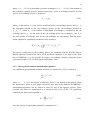
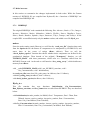
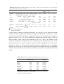
To solve Eqs. (2.5) or (2.6), the initial and boundary conditions must be specified. Initial total
aqueous concentrations of all aqueous species as a function of depth at time zero in both the
mobile and immobile regions must be defined. Concentrations of adsorbed secondary or
precipitated species must also be specified at time zero when kinetic adsorption and
precipitation/dissolution reactions are considered.
Possible boundary conditions include first-type (or Dirichlet type) boundary conditions
defining a prescribed boundary concentration, and third-type (or Cauchy type) boundary
conditions defining a prescribed boundary solute flux. At an impermeable boundary (i.e.,
where q=0) or at a boundary where water flows out of the domain, the third-type boundary
condition reduces to a second-type (Neumann type) boundary condition.
2.3 Heat transport in the vadose zone
2.3.1
The heat transport equation
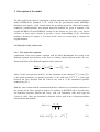
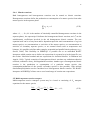
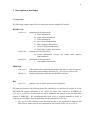
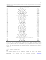
The one-dimensional heat transport equation (neglecting water vapour diffusion) is given by
∂C p (θ )T
∂qT
= ∂ ⎡ λ (θ ) ∂T ⎤ − C w
− C w ST
∂t
∂x ⎣
∂x ⎦
∂x
(2.9)
where λ(θ) is the apparent thermal conductivity of the soil [MLT-3K-1], and Cp(θ) and Cw are
volumetric heat capacities of the porous medium and the liquid phase, respectively, [ML-1T2 -1
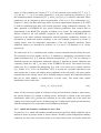
K ]. The volumetric heat capacity of the porous medium is estimated based on its
constituents (de Vries, 1963) as follows
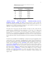
C p (θ ) = C nθ n + C oθ o + C wθ + C aθ v
(2.10)
where Cn, Co, and Ca are the volumetric heat capacities of the solid phase, the organic matter,
and the gas phase, respectively, [ML-1T-2K-1], and θn, θo, and θv are the volumetric fractions of
the solid phase, the organic matter, and the gas phase, respectively [L3L-3]. The apparent
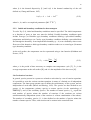
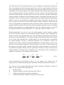
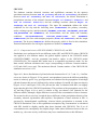
thermal conductivity is defined as (de Marsily, 1986)
λ (θ ) = λ0 (θ ) + β t C w q
(2.11)