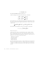
1
RF Module User´s Guide VERSION 4.3 RF Module User’s Guide 1998–2012 COMSOL Protected by U.S. Patents 7,519,518; 7,596,474; and 7,623,991. Patents pending. This Documentation and the Programs described herein are furnished under the COMSOL Software License Agreement (www.comsol.com/sla) and may be used or copied only under the terms of the license agreement. COMSOL, COMSOL Desktop, COMSOL Multiphysics, and LiveLink are registered trademarks or trademarks of COMSOL AB. Other product or brand names are trademarks or registered trademarks of their respective holders. Version: May 2012 COMSOL 4.3 Contact Information Visit www.comsol.com/contact for a searchable list of all COMSOL offices and local representatives. From this web page, search the contacts and find a local sales representative, go to other COMSOL websites, request information and pricing, submit technical support queries, subscribe to the monthly eNews email newsletter, and much more. If you need to contact Technical Support, an online request form is located at www.comsol.com/support/contact. Other useful links include: • Technical Support www.comsol.com/support • Software updates: www.comsol.com/support/updates • Online community: www.comsol.com/community • Events, conferences, and training: www.comsol.com/events • Tutorials: www.comsol.com/products/tutorials • Knowledge Base: www.comsol.com/support/knowledgebase Part No. CM021001 C o n t e n t s Chapter 1: Introduction About the RF Module 10 What Can the RF Module Do?. . . . . . . . . . . . . . . . . . 10 What Problems Can You Solve? . . . . . . . . . . . . . . . . . 11 RF Module Physics Guide. . . . . . . . . . . . . . . . . . . . 12 Selecting the Study Type . . . . . . . . . . . . . . . . . . . . 13 Material Properties and the Material Browser . . . . . . . . . . . . 15 The RF Module Modeling Process . . . . . . . . . . . . . . . . 16 Show More Physics Options . . . . . . . . . . . . . . . . . . 16 Where Do I Access the Documentation and Model Library? . . . . . . 18 Typographical Conventions . . . . . . . . . . . . . . . . . . . 20 Overview of the User’s Guide 23 Chapter 2: RF Modeling Preparing for RF Modeling 26 Simplifying Geometries 27 2D Models . . . . . . . . . . . . . . . . . . . . . . . . . 27 3D Models . . . . . . . . . . . . . . . . . . . . . . . . . 29 Using Efficient Boundary Conditions . . . . . . . . . . . . . . . 30 Applying Electromagnetic Sources . . . . . . . . . . . . . . . . 30 Meshing and Solving . . . . . . . . . . . . . . . . . . . . . . 31 Periodic Boundary Conditions 32 Perfectly Matched Layers (PMLs) 33 The Challenge of Open Boundaries in Radiation Problems . . . . . . . 33 PML Implementation . . . . . . . . . . . . . . . . . . . . . 34 Known Issues When Modeling Using PMLs . . . . . . . . . . . . . 36 CONTENTS |3 Scattered Field Formulation 38 Modeling with Far-Field Calculations 39 Far-Field Support in the Electromagnetic Waves, Frequency Domain Interface . 39 The Far Field Plots . . . . . . . . . . . . . . . . . . . . . . 40 S-Parameters and Ports 42 S-Parameters in Terms of Electric Field . . . . . . . . . . . . . . 42 S-Parameter Calculations in COMSOL Multiphysics: Ports . . . . . . . 43 S-Parameter Variables . . . . . . . . . . . . . . . . . . . . . 43 Port Sweeps and Touchstone Export . . . . . . . . . . . . . . . 44 Lumped Ports with Voltage Input 45 About Lumped Ports . . . . . . . . . . . . . . . . . . . . . 45 Lumped Port Parameters . . . . . . . . . . . . . . . . . . . . 46 Lumped Ports in the RF Module . . . . . . . . . . . . . . . . . 48 ECAD Import 49 Overview of the ECAD Import . . . . . . . . . . . . . . . . . 49 Importing ODB++(X) Files . . . . . . . . . . . . . . . . . . . 50 Importing GDS-II Files . . . . . . . . . . . . . . . . . . . . . 51 Importing NETEX-G Files . . . . . . . . . . . . . . . . . . . 52 ECAD Import Options . . . . . . . . . . . . . . . . . . . . 55 Meshing an Imported Geometry . . . . . . . . . . . . . . . . . 58 Troubleshooting ECAD Import . . . . . . . . . . . . . . . . . 58 Lossy Eigenvalue Calculations 60 Eigenfrequency Analysis . . . . . . . . . . . . . . . . . . . . 60 Mode Analysis . . . . . . . . . . . . . . . . . . . . . . . . 62 Connecting to Electrical Circuits 64 About Connecting Electrical Circuits to Physics Interfaces . . . . . . . 64 Connecting Electrical Circuits Using Predefined Couplings . . . . . . . 65 Connecting Electrical Circuits by User-Defined Couplings . . . . . . . 65 4 | CONTENTS Chapter 3: Electromagnetics Theory Maxwell’s Equations Introduction to Maxwell’s Equations 68 . . . . . . . . . . . . . . . 68 Constitutive Relations . . . . . . . . . . . . . . . . . . . . . 69 Potentials. . . . . . . . . . . . . . . . . . . . . . . . . . 70 Electromagnetic Energy . . . . . . . . . . . . . . . . . . . . 71 Material Properties . . . . . . . . . . . . . . . . . . . . . . 72 Boundary and Interface Conditions . . . . . . . . . . . . . . . . 73 Phasors . . . . . . . . . . . . . . . . . . . . . . . . . . 74 Special Calculations 76 S-Parameter Calculations . . . . . . . . . . . . . . . . . . . . 76 Lumped Port Parameters . . . . . . . . . . . . . . . . . . . . 79 Far-Field Calculations Theory . . . . . . . . . . . . . . . . . . 81 References . . . . . . . . . . . . . . . . . . . . . . . . . 82 Electromagnetic Quantities 83 Chapter 4: The Radio Frequency Branch The Electromagnetic Waves, Frequency Domain Interface 86 Domain, Boundary, Edge, Point, and Pair Features for the Electromagnetic Waves, Frequency Domain Interface . . . . . . . . . . . . . . . 88 Wave Equation, Electric . . . . . . . . . . . . . . . . . . . . 90 Divergence Constraint. . . . . . . . . . . . . . . . . . . . . 95 Archie’s Law . . . . . . . . . . . . . . . . . . . . . . . . 95 Porous Media . . . . . . . . . . . . . . . . . . . . . . . . 97 Far-Field Domain . . . . . . . . . . . . . . . . . . . . . . . 98 Far-Field Calculation . . . . . . . . . . . . . . . . . . . . . 99 Perfectly Matched Layers . . . . . . . . . . . . . . . . . . . . 99 Initial Values. . . . . . . . . . . . . . . . . . . . . . . . 100 Perfect Electric Conductor . . . . . . . . . . . . . . . . . . 100 Perfect Magnetic Conductor . . . . . . . . . . . . . . . . . 101 Port . . . . . . . . . . . . . . . . . . . . . . . . . . . 102 CONTENTS |5 Lumped Port . . . . . . . . . . . . . . . . . . . . . . . 105 Electric Field . . . . . . . . . . . . . . . . . . . . . . . 107 Magnetic Field . . . . . . . . . . . . . . . . . . . . . . . 108 Scattering Boundary Condition . . . . . . . . . . . . . . . . 109 Impedance Boundary Condition . . . . . . . . . . . . . . . . 110 Surface Current . . . . . . . . . . . . . . . . . . . . . . 112 Transition Boundary Condition . . . . . . . . . . . . . . . . 113 Periodic Condition . . . . . . . . . . . . . . . . . . . . . 114 Magnetic Current . . . . . . . . . . . . . . . . . . . . . 115 Edge Current . . . . . . . . . . . . . . . . . . . . . . . 116 Electric Point Dipole . . . . . . . . . . . . . . . . . . . . 116 Magnetic Point Dipole . . . . . . . . . . . . . . . . . . . . 117 Line Current (Out-of-Plane) 117 . . . . . . . . . . . . . . . . . The Electromagnetic Waves, Transient Interface 118 Domain, Boundary, Edge, Point, and Pair Conditions for the Electromagnetic Waves, Transient Interface . . . . . . . . . . . . . . . . . . 119 Wave Equation, Electric . . . . . . . . . . . . . . . . . . . 121 Initial Values. . . . . . . . . . . . . . . . . . . . . . . . 124 The Transmission Line Interface 125 Domain, Boundary, Edge, Point, and Pair Features for the Transmission Line 6 | CONTENTS Equation Interface . . . . . . . . . . . . . . . . . . . . . 127 Transmission Line Equation . . . . . . . . . . . . . . . . . . 127 Initial Values. . . . . . . . . . . . . . . . . . . . . . . . 128 Absorbing Boundary . . . . . . . . . . . . . . . . . . . . 128 Incoming Wave . . . . . . . . . . . . . . . . . . . . . . 129 Open Circuit . . . . . . . . . . . . . . . . . . . . . . . 130 Terminating Impedance . . . . . . . . . . . . . . . . . . . 130 Short Circuit . . . . . . . . . . . . . . . . . . . . . . . 132 Lumped Port . . . . . . . . . . . . . . . . . . . . . . . 132 Theory for the Electromagnetic Waves Interfaces 134 Introduction to the RF Interface Equations . . . . . . . . . . . . 134 Frequency Domain Equation . . . . . . . . . . . . . . . . . 134 Time Domain Equation . . . . . . . . . . . . . . . . . . . 140 Vector Elements . . . . . . . . . . . . . . . . . . . . . . 142 Eigenfrequency Calculations. . . . . . . . . . . . . . . . . . 142 Effective Conductivity in Porous Media and Mixtures . . . . . . . . 142 Effective Relative Permeability in Porous Media and Mixtures . . . . . 144 Archie’s Law Theory . . . . . . . . . . . . . . . . . . . . 145 Theory for the Transmission Line Interface 147 Introduction to Transmission Line Theory . . . . . . . . . . . . 147 Theory for the Transmission Line Boundary Conditions . . . . . . . 148 Chapter 5: The ACDC Branch The Electrical Circuit Interface 152 Ground Node . . . . . . . . . . . . . . . . . . . . . . . 153 Resistor . . . . . . . . . . . . . . . . . . . . . . . . . 154 Capacitor. . . . . . . . . . . . . . . . . . . . . . . . . 154 Inductor . . . . . . . . . . . . . . . . . . . . . . . . . 154 Voltage Source. . . . . . . . . . . . . . . . . . . . . . . 154 Current Source . . . . . . . . . . . . . . . . . . . . . . 155 Voltage-Controlled Voltage Source . . . . . . . . . . . . . . . 156 Voltage-Controlled Current Source . . . . . . . . . . . . . . . 156 Current-Controlled Voltage Source . . . . . . . . . . . . . . . 156 Current-Controlled Current Source . . . . . . . . . . . . . . 157 Subcircuit Definition . . . . . . . . . . . . . . . . . . . . 157 Subcircuit Instance . . . . . . . . . . . . . . . . . . . . . 158 NPN BJT . . . . . . . . . . . . . . . . . . . . . . . . . 158 n-Channel MOSFET . . . . . . . . . . . . . . . . . . . . . 158 Diode . . . . . . . . . . . . . . . . . . . . . . . . . . 159 External I vs. U . . . . . . . . . . . . . . . . . . . . . . 160 External U vs. I . . . . . . . . . . . . . . . . . . . . . . 161 External I-Terminal . . . . . . . . . . . . . . . . . . . . . 161 SPICE Circuit Import . . . . . . . . . . . . . . . . . . . . 162 Theory for the Electrical Circuit Interface 163 Electric Circuit Modeling and the Semiconductor Device Models. . . . 163 NPN Bipolar Transistor . . . . . . . . . . . . . . . . . . . 164 n-Channel MOS Transistor . . . . . . . . . . . . . . . . . . 167 Diode . . . . . . . . . . . . . . . . . . . . . . . . . . 170 CONTENTS |7 References for the Electrical Circuit Interface . . . . . . . . . . . 173 Chapter 6: The Electromagnetic Heating Branch The Microwave Heating Interface 176 Domain, Boundary, Edge, Point, and Pair Features for the Microwave Heating Interface . . . . . . . . . . . . . . . . . . . . . . . . . 179 Microwave Heating Model . . . . . . . . . . . . . . . . . . 181 Electromagnetic Heat Source . . . . . . . . . . . . . . . . . 183 Initial Values. . . . . . . . . . . . . . . . . . . . . . . . 183 Chapter 7: Glossary Glossary of Terms 8 | CONTENTS 186 1 Introduction This guide describes the RF Module, an optional add-on package for COMSOL Multiphysics with customized user interfaces and functionality optimized for the analysis of electromagnetic waves. This chapter introduces you to the capabilities of this module. A summary of the physics interfaces and where you can find documentation and model examples is also included. The last section is a brief overview with links to each chapter in this guide. • About the RF Module • Overview of the User’s Guide 9 About the RF Module In this section: • What Can the RF Module Do? • What Problems Can You Solve? • RF Module Physics Guide • Selecting the Study Type • Material Properties and the Material Browser • The RF Module Modeling Process • Show More Physics Options • Where Do I Access the Documentation and Model Library? • Typographical Conventions See Also Overview of the Physics Interfaces and Building a COMSOL Model in the COMSOL Multiphysics User’s Guide What Can the RF Module Do? The RF Module solves problems in the general field of electromagnetic waves, such as RF and microwave applications, optics, and photonics. The underlying equations for electromagnetics are automatically available in all of the physics interfaces—a feature unique to COMSOL Multiphysics. This also makes nonstandard modeling easily accessible. The module is useful for component design in virtually all areas where you find electromagnetic waves, such as: • Antennas • Waveguides and cavity resonators in microwave engineering • Optical fibers • Photonic waveguides • Photonic crystals • Active devices in photonics 10 | CHAPTER 1: INTRODUCTION The physics interfaces cover the following types of electromagnetics field simulations and handle time-harmonic, time-dependent, and eigenfrequency/eigenmode problems: • In-plane, axisymmetric, and full 3D electromagnetic wave propagation • Full vector mode analysis in 2D and 3D Material properties include inhomogeneous and fully anisotropic materials, media with gains or losses, and complex-valued material properties. In addition to the standard postprocessing features, the module supports direct computation of S-parameters and far-field patterns. You can add ports with a wave excitation with specified power level and mode type, and add PMLs (perfectly matched layers) to simulate electromagnetic waves that propagate into an unbounded domain. For time-harmonic simulations, you can use the scattered wave or the total wave. Using the multiphysics capabilities of COMSOL Multiphysics you can couple simulations with heat transfer, structural mechanics, fluid flow formulations, and other physical phenomena. This module also has interfaces for circuit modeling, a SPICE interface, and support for importing ECAD drawings. What Problems Can You Solve? QUASI-STATIC AND HIGH FREQUENCY MODELING One major difference between quasi-static and high-frequency modeling is that the formulations depend on the electrical size of the structure. This dimensionless measure is the ratio between the largest distance between two points in the structure divided by the wavelength of the electromagnetic fields. For simulations of structures with an electrical size in the range up to 1/10, quasi-static formulations are suitable. The physical assumption of these situations is that wave propagation delays are small enough to be neglected. Thus, phase shifts or phase gradients in fields are caused by materials and/or conductor arrangements being inductive or capacitive rather than being caused by propagation delays. For electrostatic, magnetostatic, and quasi-static electromagnetics, use the AC/DC Module, a COMSOL Multiphysics add-on module for low-frequency electromagnetics. ABOUT THE RF MODULE | 11 When propagation delays become important, it is necessary to use the full Maxwell equations for high-frequency electromagnetic waves. They are appropriate for structures of electrical size 1/100 and larger. Thus, an overlapping range exists where you can use both the quasi-static and the full Maxwell physics interfaces. Independently of the structure size, the module accommodates any case of nonlinear, inhomogeneous, or anisotropic media. It also handles materials with properties that vary as a function of time as well as frequency-dispersive materials. RF Module Physics Guide The interfaces in this module form a complete set of simulation tools for electromagnetic wave simulations. Use the Model Wizard to select the physics interface and study type when starting to build a new model. You can add interfaces and studies to an existing model throughout the design process. Refer to the COMSOL Multiphysics User’s Guide for detailed instructions. In addition to the interfaces included with the basic COMSOL license, the interfaces below are included with the RF Module and available in the indicated space dimension. All interfaces are available in 2D and 3D. In 2D there are in-plane formulations for problems with a planar symmetry as well as axisymmetric formulations for problems with a cylindrical symmetry. 2D mode analysis of waveguide cross sections with out-of-plane propagation is also supported. See Simplifying Geometries for more information about selecting the right space dimension for the model. • Study Types in the COMSOL Multiphysics Reference Guide See Also • Available Study Types in the COMSOL Multiphysics User’s Guide PHYSICS ICON TAG SPACE DIMENSION PRESET STUDIES cir Not space dependent stationary; frequency domain; time dependent AC/DC Electrical Circuit 12 | CHAPTER 1: INTRODUCTION PHYSICS ICON TAG SPACE DIMENSION PRESET STUDIES mh 3D, 2D, 2D axisymmetric stationary; frequency domain; time dependent; boundary mode analysis; frequency-stationary; frequency transient Electromagnetic Waves, Frequency Domain emw 3D, 2D, 2D axisymmetric eigenfrequency; frequency domain; frequency-domain modal; boundary mode analysis Electromagnetic Waves, Transient temw 3D, 2D, 2D axisymmetric eigenfrequency; time dependent; time dependent modal Transmission Line tl 3D, 2D, 1D eigenfrequency; frequency domain Heat Transfer Electromagnetic Heating Microwave Heating Radio Frequency Selecting the Study Type To carry out different kinds of simulations for a given set of parameters in a physics interface, you can select, add, and change the Study Types at almost every stage of modeling (see the COMSOL Multiphysics User’s Guide for instructions). The available study types are listed in Table 1-1 with column definitions after the table. • Study Types in the COMSOL Multiphysics Reference Guide See Also • Available Study Types in the COMSOL Multiphysics User’s Guide ABOUT THE RF MODULE | 13 TABLE 1-1: RF MODULE PHYSICS INTERFACE DEPENDENT VARIABLES AND PRESET STUDIES Electromagnetic Waves, Transient temw A all 3 mh T, J, E all 3 mwp See the Plasma Module documentation for details. FREQUENCY TRANSIENT all 3 FREQUENCY STATIONARY E BOUNDARY MODE ANALYSIS emw FREQUENCY DOMAIN MODAL Electromagnetic Waves, Frequency Domain EIGENFREQUENCY PRESET STUDIES FREQUENCY DOMAIN FIELD COMP. TIME DEPENDENT MODEL DEP. VAR. TIME DEPENDENT NAME MAGNETIC FIELD AND ELECTRIC FIELDS THE BRANCH AND PHYSICS INTERFACE RADIO FREQUENCY HEAT TRANSFER Microwave Heating PLASMA Microwave Plasma COMPARING THE TIME DEPENDENT AND FREQUENCY DOMAIN STUDIES When variations in time are present there are two main approaches to represent the time dependence. The most straightforward is to solve the problem by calculating the changes in the solution for each time step; that is, solving using the Time Dependent study (available with the Electromagnetic Waves, Transient interface). However, this approach can be time consuming if small time steps are necessary for the desired accuracy. It is necessary when the inputs are transients like turn-on and turn-off sequences. However, if the Frequency Domain study available with the Electromagnetic Waves, Frequency Domain interface is used, this allows you to efficiently simplify and assume that all variations in time occur as sinusoidal signals. Then the problem is time-harmonic and in the frequency domain. Thus you can formulate it as a stationary problem with complex-valued solutions. The complex value represents both the amplitude and the phase of the field, while the frequency is specified as a scalar model input, usually provided by the solver. This approach is useful because, combined with 14 | CHAPTER 1: INTRODUCTION Fourier analysis, it applies to all periodic signals with the exception of nonlinear problems. Examples of typical frequency domain simulations are wave-propagation problems like waveguides and antennas. For nonlinear problems you can apply a Frequency Domain study after a linearization of the problem, which assumes that the distortion of the sinusoidal signal is small. Use a Time Dependent study when the nonlinear influence is strong, or if you are interested in the harmonic distortion of a sine signal. It may also be more efficient to use a time dependent study if you have a periodic input with many harmonics, like a square-shaped signal. Material Properties and the Material Browser All physics interfaces in the RF Module support the use of the COMSOL Multiphysics material database libraries. The electromagnetic material properties that can be stored in the materials database are: • The electrical conductivity • The relative permittivity • The relative permeability • The refractive index The physics-specific domain material properties are by default taken from the material specification. The material properties are inputs to material laws or constitutive relations that are defined on the feature level below the physics interface node in the model tree. There is one editable default domain feature (wave equation) that initially represents a linear isotropic material. Domains with different material laws are specified by adding additional features. Some of the domain parameters can either be a scalar or a matrix (tensor) depending on whether the material is isotropic or anisotropic. In a similar way, boundary, edge, and point settings are specified by adding the corresponding features. A certain feature might require one or several fields to be specified, while others generate the conditions without user-specified fields. See Also Materials and Modeling Anisotropic Materials in the COMSOL Multiphysics User’s Guide ABOUT THE RF MODULE | 15 The RF Module Modeling Process The modeling process has these main steps, which (excluding the first step), correspond to the branches displayed in the Model Builder in the COMSOL Desktop environment. 1 Selecting the appropriate physics interface or predefined multiphysics coupling in the Model Wizard. 2 Defining model parameters and variables in the Definitions branch ( 3 Drawing or importing the model geometry in the Geometry branch ( 4 Assigning material properties to the geometry in the Materials branch ( ). ). ). 5 Setting up the model equations and boundary conditions in the physics interfaces branch. 6 Meshing in the Mesh branch ( ). 7 Setting up the study and computing the solution in the Study branch ( 8 Analyzing and visualizing the results in the Results branch ( ). ). Even after a model is defined, you can edit to input data, equations, boundary conditions, geometry—the equations and boundary conditions are still available through associative geometry—and mesh settings. You can restart the solver, for example, using the existing solution as the initial condition or initial guess. It is also easy to add another interface to account for a phenomenon not previously described in a model. • Building a COMSOL Model in the COMSOL Multiphysics User’s Guide See Also • RF Module Physics Guide • Selecting the Study Type Show More Physics Options There are several features available on many physics interfaces or individual nodes. This section is a short overview of the options and includes links to the COMSOL 16 | CHAPTER 1: INTRODUCTION Multiphysics User’s Guide or COMSOL Multiphysics Reference Guide where additional information is available. Important Tip The links to the features described in the COMSOL Multiphysics User’s Guide and COMSOL Multiphysics Reference Guide do not work in the PDF, only from within the online help. To locate and search all the documentation for this information, in COMSOL, select Help>Documentation from the main menu and either enter a search term or look under a specific module in the documentation tree. To display additional features for the physics interfaces and feature nodes, click the Show button ( ) on the Model Builder and then select the applicable option. After clicking the Show button ( ), some sections display on the settings window when a node is clicked and other features are available from the context menu when a node is right-clicked. For each, the additional sections that can be displayed include Equation, Advanced Settings, Discretization, Consistent Stabilization, and Inconsistent Stabilization. ) in the Model Builder to always show You can also click the Expand Sections button ( ) and select Reset to Default to reset to some sections or click the Show button ( display only the Equation and Override and Contribution sections. For most physics nodes, both the Equation and Override and Contribution sections are ) and then select Equation View to display always available. Click the Show button ( the Equation View node under all physics nodes in the Model Builder. Availability of each feature, and whether it is described for a particular physics node, is based on the individual physics selected. For example, the Discretization, Advanced ABOUT THE RF MODULE | 17 Settings, Consistent Stabilization, and Inconsistent Stabilization sections are often described individually throughout the documentation as there are unique settings. SECTION CROSS REFERENCE LOCATION IN COMSOL MULTIPHYSICS USER GUIDE OR REFERENCE GUIDE Show More Options and Expand Sections • Showing and Expanding Advanced Physics Sections User’s Guide • The Model Builder Window Discretization • Show Discretization User’s Guide • Element Types and Discretization • Finite Elements Reference Guide • Discretization of the Equations Discretization - Splitting of complex variables Compile Equations Reference Guide Pair Selection • Identity and Contact Pairs User’s Guide • Specifying Boundary Conditions for Identity Pairs Consistent and Inconsistent Stabilization Show Stabilization User’s Guide • Stabilization Techniques Reference Guide • Numerical Stabilization Geometry Working with Geometry User’s Guide Constraint Settings Using Weak Constraints User’s Guide Where Do I Access the Documentation and Model Library? A number of Internet resources provide more information about COMSOL Multiphysics, including licensing and technical information. The electronic 18 | CHAPTER 1: INTRODUCTION documentation, Dynamic Help, and the Model Library are all accessed through the COMSOL Desktop. Important If you are reading the documentation as a PDF file on your computer, the blue links do not work to open a model or content referenced in a different user’s guide. However, if you are using the online help in COMSOL Multiphysics, these links work to other modules, model examples, and documentation sets. THE DOCUMENTATION The COMSOL Multiphysics User’s Guide and COMSOL Multiphysics Reference Guide describe all interfaces and functionality included with the basic COMSOL Multiphysics license. These guides also have instructions about how to use COMSOL Multiphysics and how to access the documentation electronically through the COMSOL Multiphysics help desk. To locate and search all the documentation, in COMSOL Multiphysics: • Press F1 for Dynamic Help, • Click the buttons on the toolbar, or • Select Help>Documentation ( ) or Help>Dynamic Help ( ) from the main menu and then either enter a search term or look under a specific module in the documentation tree. THE MODEL LIBRARY Each model comes with documentation that includes a theoretical background and step-by-step instructions to create the model. The models are available in COMSOL as MPH-files that you can open for further investigation. You can use the step-by-step instructions and the actual models as a template for your own modeling and applications. SI units are used to describe the relevant properties, parameters, and dimensions in most examples, but other unit systems are available. ) from the main menu, and To open the Model Library, select View>Model Library ( then search by model name or browse under a module folder name. Click to highlight any model of interest, and select Open Model and PDF to open both the model and the documentation explaining how to build the model. Alternatively, click the Dynamic ABOUT THE RF MODULE | 19 Help button ( ) or select Help>Documentation in COMSOL to search by name or browse by module. The model libraries are updated on a regular basis by COMSOL in order to add new models and to improve existing models. Choose View>Model Library Update ( ) to update your model library to include the latest versions of the model examples. If you have any feedback or suggestions for additional models for the library (including those developed by you), feel free to contact us at [email protected]. CONT ACT ING COMSOL BY EMAIL For general product information, contact COMSOL at [email protected]. To receive technical support from COMSOL for the COMSOL products, please contact your local COMSOL representative or send your questions to [email protected]. An automatic notification and case number is sent to you by email. COMSOL WEB SITES Main Corporate web site www.comsol.com Worldwide contact information www.comsol.com/contact Technical Support main page www.comsol.com/support Support Knowledge Base www.comsol.com/support/knowledgebase Product updates www.comsol.com/support/updates COMSOL User Community www.comsol.com/community Typographical Conventions All COMSOL user’s guides use a set of consistent typographical conventions that make it easier to follow the discussion, understand what you can expect to see on the graphical user interface (GUI), and know which data must be entered into various data-entry fields. 20 | CHAPTER 1: INTRODUCTION In particular, these conventions are used throughout the documentation: CONVENTION EXAMPLE text highlighted in blue Click text highlighted in blue to go to other information in the PDF. When you are using the online help desk in COMSOL Multiphysics, these links also work to other modules, model examples, and documentation sets. boldface font A boldface font indicates that the given word(s) appear exactly that way on the COMSOL Desktop (or, for toolbar buttons, in the corresponding tip). For example, the Model ) is often referred to and this is the Builder window ( window that contains the model tree. As another example, the instructions might say to click the Zoom Extents button ( ), and this means that when you hover over the button with your mouse, the same label displays on the COMSOL Desktop. Forward arrow symbol > The forward arrow symbol > is instructing you to select a series of menu items in a specific order. For example, Options>Preferences is equivalent to: From the Options menu, choose Preferences. Code (monospace) font A Code (monospace) font indicates you are to make a keyboard entry in the user interface. You might see an instruction such as “Enter (or type) 1.25 in the Current density field.” The monospace font also is an indication of programming code or a variable name. Italic Code (monospace) font An italic Code (monospace) font indicates user inputs and parts of names that can vary or be defined by the user. Arrow brackets <> following the Code (monospace) or Code (italic) fonts The arrow brackets included in round brackets after either a monospace Code or an italic Code font means that the content in the string can be freely chosen or entered by the user, such as feature tags. For example, model.geom(<tag>) where <tag> is the geometry’s tag (an identifier of your choice). When the string is predefined by COMSOL, no bracket is used and this indicates that this is a finite set, such as a feature name. KEY TO THE GRAPHICS Throughout the documentation, additional icons are used to help navigate the information. These categories are used to draw your attention to the information ABOUT THE RF MODULE | 21 based on the level of importance, although it is always recommended that you read these text boxes. ICON NAME DESCRIPTION Caution A Caution icon is used to indicate that the user should proceed carefully and consider the next steps. It might mean that an action is required, or if the instructions are not followed, that there will be problems with the model solution. Important An Important icon is used to indicate that the information provided is key to the model building, design, or solution. The information is of higher importance than a note or tip, and the user should endeavor to follow the instructions. Note A Note icon is used to indicate that the information may be of use to the user. It is recommended that the user read the text. Tip A Tip icon is used to provide information, reminders, short cuts, suggestions of how to improve model design, and other information that may or may not be useful to the user. See Also The See Also icon indicates that other useful information is located in the named section. If you are working on line, click the hyperlink to go to the information directly. When the link is outside of the current PDF document, the text indicates this, for example See The Laminar Flow Interface in the COMSOL Multiphysics User’s Guide. Note that if you are in COMSOL Multiphysics’ online help, the link will work. Model The Model icon is used in the documentation as well as in COMSOL Multiphysics from the View>Model Library menu. If you are working online, click the link to go to the PDF version of the step-by-step instructions. In some cases, a model is only available if you have a license for a specific module. These examples occur in the COMSOL Multiphysics User’s Guide. The Model Library path describes how to find the actual model in COMSOL Multiphysics, for example If you have the RF Module, see Radar Cross Section: Model Library path RF_Module/Tutorial_Models/radar_cross_section Space Dimension 22 | CHAPTER 1: INTRODUCTION Another set of icons are also used in the Model Builder—the model space dimension is indicated by 0D , 1D , 1D axial symmetry , 2D , 2D axial symmetry , and 3D icons. These icons are also used in the documentation to clearly list the differences to an interface, feature node, or theory section, which are based on space dimension. Overview of the User’s Guide The RF Module User’s Guide gets you started with modeling using COMSOL Multiphysics. The information in this guide is specific to this module. Instructions how to use COMSOL in general are included with the COMSOL Multiphysics User’s Guide. Tip As detailed in the section Where Do I Access the Documentation and Model Library? this information is also searchable from the COMSOL Multiphysics software Help menu. TA B L E O F C O N T E N T S , G L O S S A R Y, A N D I N D E X To help you navigate through this guide, see the Contents, Glossary, and Index. MODELING WITH THE RF MODULE The RF Modeling chapter familiarize you with the modeling procedures. A number of models available through the Model Library also illustrate the different aspects of the simulation process. Topics include Preparing for RF Modeling, Simplifying Geometries, Perfectly Matched Layers (PMLs), and Scattered Field Formulation. RF THEORY The Electromagnetics Theory chapter contains a review of the basic theory of electromagnetics, starting with Maxwell’s Equations, and the theory for some Special Calculations: S-parameters, lumped port parameters, and far-field analysis. There is also a list of Electromagnetic Quantities with their SI units and symbols. RADIO FREQUENCY The Radio Frequency Branch chapter describes The Electromagnetic Waves, Frequency Domain Interface, which analyzes frequency domain electromagnetic waves, and uses time-harmonic and eigenfrequency or eigenmode (2D only) studies, boundary mode analysis and frequency domain modal. It also describes The Electromagnetic Waves, Transient Interface, which supports the time dependent study type. The underlying theory is also included at the end of the chapter. O V E R V I E W O F T H E U S E R ’S G U I D E | 23 ELECTRICAL CIRCUIT The ACDC Branch chapter describes The Electrical Circuit Interface, which simulates the current in a conductive and capacitive material under the influence of an electric field. All three study types (stationary, frequency domain, and time-dependent) are available. The underlying theory is also included at the end of the chapter. H E A T TR A N S F E R The Electromagnetic Heating Branch chapter describes the Microwave Heating interface, which combines the features of an Electromagnetic Waves, Frequency Domain interface from the RF Module with the Heat Transfer interface. The predefined interaction adds the electromagnetic losses from the electromagnetic waves as a heat source and solves frequency domain (time-harmonic) electromagnetic waves in conjunction with stationary or transient heat transfer. This interface is based on the assumption that the electromagnetic cycle time is short compared to the thermal time scale (adiabatic assumption). The underlying theory is also included at the end of the chapter. 24 | CHAPTER 1: INTRODUCTION 2 RF Modeling The goal of this chapter is to familiarize you with the modeling procedure in the RF Module. A number of models available through the Model Library also illustrate the different aspects of the simulation process. In this chapter: • Preparing for RF Modeling • Simplifying Geometries • Periodic Boundary Conditions • Perfectly Matched Layers (PMLs) • Scattered Field Formulation • Modeling with Far-Field Calculations • S-Parameters and Ports • Lumped Ports with Voltage Input • ECAD Import • Lossy Eigenvalue Calculations • Connecting to Electrical Circuits 25 Preparing for RF Modeling Several modeling topics are described in this section that may not be found in ordinary textbooks on electromagnetic theory. This chapter is intended to help answer questions such as: • Which spatial dimension should I use: 3D, 2D axial symmetry, or 2D? • Is my problem suited for time dependent or frequency domain formulations? • Can I use a quasi-static formulation or do I need wave propagation? • What sources can I use to excite the fields? • When do I need to resolve the thickness of thin shells and when can I use boundary conditions? • What is the purpose of the model? • What information do I want to extract from the model? Increasing the complexity of a model to make it more accurate usually makes it more expensive to simulate. A complex model is also more difficult to manage and interpret than a simple one. Keep in mind that it can be more accurate and efficient to use several simple models instead of a single, complex one. See Also 26 | • Overview of the Physics Interfaces and Building a COMSOL Model in the COMSOL Multiphysics User’s Guide CHAPTER 2: RF MODELING Simplifying Geometries Most of the problems that are solved with COMSOL Multiphysics are three-dimensional (3D) in the real world. In many cases, it is sufficient to solve a two-dimensional (2D) problem that is close to or equivalent to the real problem. Furthermore, it is good practice to start a modeling project by building one or several 2D models before going to a 3D model. This is because 2D models are easier to modify and solve much faster. Thus, modeling mistakes are much easier to find when working in 2D. Once the 2D model is verified, you are in a much better position to build a 3D model. In this section: • 2D Models • 3D Models • Using Efficient Boundary Conditions • Applying Electromagnetic Sources • Meshing and Solving 2D Models The text below is a guide to some of the common approximations made for 2D models. Remember that the modeling in 2D usually represents some 3D geometry under the assumption that nothing changes in the third dimension. CARTESIAN COORDINATES In this case a cross section is viewed in the xy-plane of the actual 3D geometry. The geometry is mathematically extended to infinity in both directions along the z-axis, assuming no variation along that axis. All the total flows in and out of boundaries are per unit length along the z-axis. A simplified way of looking at this is to assume that the geometry is extruded one unit length from the cross section along the z-axis. The total flow out of each boundary is then from the face created by the extruded boundary (a boundary in 2D is a line). There are usually two approaches that lead to a 2D cross-section view of a problem. The first approach is when it is known that there is no variation of the solution in one particular dimension. SIMPLIFYING GEOMETRIES | 27 This is shown in the model H-Bend Waveguide 2D, where the electric field only has one component in the z direction and is constant along that axis. The second approach is when there is a problem where the influence of the finite extension in the third dimension can be neglected. Figure 2-1: The cross sections and their real geometry for Cartesian coordinates and cylindrical coordinates (axial symmetry). H-Bend Waveguide 2D: Model Library path RF_Module/ Model RF_and_Microwave_Engineering/h_bend_waveguide_2d AXIAL SYMMETRY (CYLINDRICAL COORDINATES) If the 3D geometry can be constructed by revolving a cross section around an axis, and if no variations in any variable occur when going around the axis of revolution, then use an axisymmetric physics interface. The spatial coordinates are called r and z, where r is the radius. The flow at the boundaries is given per unit length along the third dimension. Because this dimension is a revolution all flows must be multiplied with r, where is the revolution angle (for example, 2 for a full turn). Conical Antenna: Model Library path RF_Module/ Model 28 | RF_and_Microwave_Engineering/conical_antenna CHAPTER 2: RF MODELING Important When using the axisymmetric versions, the horizontal axis represents the radial (r) direction and the vertical axis the z direction, and the geometry in the right half-plane (that is, for positive r only) must be created. The physical quantities used are the electric field, E and the magnetic potential, A. PO LA RIZATION IN 2D In addition to selecting 2D or 2D axisymmetry when you start building the model, the main physics interface node (Electromagnetic Waves, Frequency Domain or Electromagnetic Waves, Transient) in the model tree offers a choice in the settings section of electric field components to solve for. The available choices are Out-of-plane vector, In-plane vector and Three-component vector. This choice determines what polarizations can be handled. For example; as you are solving for the electric field, a 2D TM (out-of-plane H field) model requires choosing In-plane vector as then the electric field components are in the modeling plane. 3D Models Although COMSOL Multiphysics fully supports arbitrary 3D geometries, it is important to simplify the problem. This is because 3D models often require more computer power, memory, and time to solve. The extra time spent on simplifying a model is probably well spent when solving it. Below are a few issues that need to be addressed before starting to implement a 3D model in the RF Module. • Check if it is possible to solve the problem in 2D. Given that the necessary approximations are small, the solution is more accurate in 2D, because a much denser mesh can be used. • Look for symmetries in the geometry and model. Many problems have planes where the solution is the same on both sides of the plane. A good way to check this is to flip the geometry around the plane, for example, by turning it up-side down around the horizontal plane. Then remove the geometry below the plane if no differences are observed between the two cases regarding geometry, materials, and sources. Boundaries created by the cross section between the geometry and this plane need a symmetry boundary condition, which is available in all 3D physics interfaces. • There are also cases when the dependence along one direction is known, and it can be replaced by an analytical function. Use this approach either to convert 3D to 2D or to convert a layer to a boundary condition. SIMPLIFYING GEOMETRIES | 29 Using Efficient Boundary Conditions An important technique to minimize the problem size is to use efficient boundary conditions. Truncating the geometry without introducing too large errors is one of the great challenges in modeling. Below are a few suggestions of how to do this. They apply to both 2D and 3D problems. • Many models extend to infinity or may have regions where the solution only undergoes small changes. This problem is addressed in two related steps. First, the geometry needs to be truncated in a suitable position. Second, a suitable boundary condition needs to be applied there. For static and quasi-static models, it is often possible to assume zero fields at the open boundary, provided that this is at a sufficient distance away from the sources. For radiation problems, special low-reflecting boundary conditions need to be applied. This boundary should be in the order of a few wavelengths away from any source. A more accurate option is to use perfectly matched layers (PMLs). PMLs are layers that absorbs all radiated waves with small reflections. • Replace thin layers with boundary conditions where possible. There are several types of boundary conditions in COMSOL Multiphysics suitable for such replacements. For example, replace materials with high conductivity by the perfect electric conductor (PEC) boundary condition. • Use boundary conditions for known solutions. For example, an antenna aperture can be modeled as an equivalent surface current density on a 2D face (boundary) in a 3D model. Applying Electromagnetic Sources Electromagnetic sources can be applied in many different ways. The typical options are boundary sources, line sources, and point sources, where point sources in 2D formulations are equivalent to line sources in 3D formulations. The way sources are imposed can have an impact on what quantities can be computed from the model. For example, a line source in an electromagnetic wave model represents a singularity and the magnetic field does not have a finite value at the position of the source. In a COMSOL Multiphysics model, the magnetic field of a line source has a finite but mesh-dependent value. In general, using volume or boundary sources is more flexible than using line sources or point sources, but the meshing of the source domains becomes more expensive. 30 | CHAPTER 2: RF MODELING Meshing and Solving The finite element method approximates the solution within each element, using some elementary shape function that can be constant, linear, or of higher order. Depending on the element order in the model, a finer or coarser mesh is required to resolve the solution. In general, there are three problem-dependent factors that determine the necessary mesh resolution: • The first is the variation in the solution due to geometrical factors. The mesh generator automatically generates a finer mesh where there is a lot of fine geometrical details. Try to remove such details if they do not influence the solution, because they produce a lot of unnecessary mesh elements. • The second is the skin effect or the field variation due to losses. It is easy to estimate the skin depth from the conductivity, permeability, and frequency. At least two linear elements per skin depth are required to capture the variation of the fields. If the skin depth is not studied or a very accurate measure of the dissipation loss profile is not needed, replace regions with a small skin depth with a boundary condition, thereby saving elements. If it is necessary to resolve the skin depth, the boundary layer meshing technique can be a convenient way to get a dense mesh near a boundary. • The third and last factor is the wavelength. To resolve a wave properly, it is necessary to use about 10 linear (or five 2nd order) elements per wavelength. Keep in mind that the wavelength depends on the local material properties. In the COMSOL Multiphysics User’s Guide: • Generating a Boundary Layer Mesh See Also • Solvers and Study Types SOLVERS In most cases the solver sequence generated by COMSOL Multiphysics can be used. The choice of solver is optimized for the typical case for each physics interface and study type in the RF Module. However, in special cases tuning the solver settings may be required. This is especially important for 3D problems because they can require a large amount of memory. For large 3D problems, a 64-bit platform may be needed. SIMPLIFYING GEOMETRIES | 31 Periodic Boundary Conditions The RF Module has a dedicated Periodic Condition. The periodic condition can identify simple mappings on plane source and destination boundaries of equal shape. The destination can also be rotated with respect to the source. There are three types of periodic conditions available (only the first two for transient analysis): • Continuity—The tangential components of the solution variables are equal on the source and destination. • Antiperiodicity—The tangential components have opposite signs. • Floquet periodicity—There is a phase shift between the tangential components. The phase shift is determined by a wave vector and the distance between the source and destination. Floquet periodicity is typically used for models involving plane waves interacting with periodic structures. Periodic boundary conditions must have compatible meshes. Note Model If more advanced periodic boundary conditions are required, for example, when there is a known rotation of the polarization from one boundary to another, see Model Couplings in the COMSOL Multiphysics User’s Guide for tools to define more general mappings between boundaries. To learn how to use the Copy Mesh feature to ensure that the mesh on the destination boundary is identical to that on the source boundary, see Fresnel Equations: Model Library path RF_Module/Verification_Models/ fresnel_equations. In the COMSOL Multiphysics User’s Guide: • Periodic Condition • Destination Selection See Also • Using Periodic Boundary Conditions • Periodic Boundary Condition Example 32 | CHAPTER 2: RF MODELING Perfectly Matched Layers (PMLs) In this section: • The Challenge of Open Boundaries in Radiation Problems • PML Implementation • Known Issues When Modeling Using PMLs For examples on using perfectly matched layers, use any of the following models in the RF Module Model Library: • Tutorial Models/Radar Cross Section (2D, cylindrical PML) Model • Tutorial Models/RF Coil (3D, spherical PML with swept mesh). • RF and Microwave Engineering/Balanced Patch Antenna for 6 GHz (3D, spherical PML). The Challenge of Open Boundaries in Radiation Problems One of the challenges in finite element modeling is how to treat open boundaries in radiation problems. This module offers two closely related types of absorbing boundary conditions, the scattering boundary condition and the port boundary condition. The scattering boundary condition is a first order absorbing boundary condition for a plane wave or (optionally) a cylindrical or spherical wave, whereas a port boundary condition is a perfectly absorbing condition for general modes of a known shape, provided that the correct mode shape and the propagation constant are supplied. Several port boundary condition features representing an expansion into mutually orthogonal modes is also allowed and can be used to account for higher diffraction orders from a grating or be used to truncate a waveguide operated in the multimode regime. However, in many scattering and antenna-modeling problems, the outgoing radiation cannot be described as a plane wave with a well-known direction of propagation or as a known, finite modal expansion. In such situations, consider using perfectly matched layers (PMLs). A PML is not, strictly speaking, a boundary condition but an additional domain that absorbs the incident radiation without producing reflections. It provides good performance for a wide range of incidence angles and is not particularly sensitive to the PERFECTLY MATCHED LAYERS (PMLS) | 33 shape of the wave fronts. The PML formulation can be deduced from Maxwell’s equations by introducing a complex-valued coordinate transformation under the additional requirement that the wave impedance should remain unaffected (Ref. 1). The following section describes how to use the semiautomatic frequency domain PMLs in the RF Module to create planar, cylindrical, and spherical PMLs. Transient PMLs are not supported. REFERENCE 1. Jianming Jin, The Finite Element Method in Electromagnetics, 2nd ed., Wiley-IEEE Press, 2002. PML Implementation The RF Module uses the following coordinate transform for the general coordinate variable t. t n t' = ------- 1 – i F w (2-1) The coordinate, t, and the width of the PML region, w, are geometrical parameters that are automatically extracted for each region. The other parameters are the PML scaling factor F and the PML order n that can be modified in the PML feature (both default to unity). To avoid a nonlinear dependence in the eigenvalue, the wavelength, , is removed from the scaling expression when computing an eigenfrequency study. The software automatically computes the value for w and the orientation of the transform for PML regions that are Cartesian, cylindrical, or spherical. However, there is no check that the geometry of the region is correct, so it is important to draw a proper geometry and select the corresponding region type. Typical examples of PML regions that work nicely are shown in the figures for three of the PML types below. The supported PML types are: • Cartesian—PMLs absorbing in Cartesian coordinate directions. It is available in 2D and 3D (Figure 2-2). • Cylindrical—PMLs absorbing in cylindrical coordinate directions from a specified axis. It is available in 3D, 2D, and 2D axisymmetry. In axisymmetry, the cylinder axis is the z-axis (Figure 2-3). 34 | CHAPTER 2: RF MODELING • Spherical—PMLs absorbing in the radial direction from a specified center point. It is available in 2D axisymmetry and 3D (Figure 2-4). • General—General PMLs or domain scaling with user-defined coordinate transformations. Figure 2-2: A cube surrounded by typical PML regions of the type “Cartesian.” Figure 2-3: A cylinder surrounded by typical cylindrical PML regions. PERFECTLY MATCHED LAYERS (PMLS) | 35 Figure 2-4: A sphere surrounded by a typical spherical PML region. GENERAL SCALING With manual control of the scaling, the geometric parameters that define the stretching are added as subnodes labeled Manual Scaling. These subnodes have no effect unless the type of the Perfectly Matched Layers node is set to General. Each Manual Scaling subnode has three parameters: the scaling direction arot, the geometric width r , and the coordinate at interface rI. The first parameter sets the direction from the interface to the outer boundary, the second parameter sets the width of the region, and the last parameter sets an arbitrary coordinate at the interface. When going from any of the other types to the general type, Manual Scaling subnodes are automatically added that represent stretching of the previous type. Known Issues When Modeling Using PMLs When modeling with PMLs, be aware of the following: • A separate Perfectly Matched Layers node must be used for each isolated PML domain. That is, to use one and the same Perfectly Matched Layers node, all PML domains must be in contact with each other. Otherwise the PMLs do not work properly. • The coordinate scaling resulting from PMLs also yields an equivalent scaling of the mesh that may effectively result in a poor element quality. (The element quality displayed by the mesh statistics feature does not account for this effect.) This typically happens when the geometrical thickness of the PML deviates much from one wavelength (local wavelength rather than free space wavelength). The poor element quality causes poor convergence for iterative solvers and make the problem ill-conditioned in general. Especially vector element formulations (the ones using 36 | CHAPTER 2: RF MODELING two or more components of a vector field variable) are sensitive to low element quality. For this reason, it is strongly recommended to use swept meshing in the PML domains. The sweep direction should be selected the same as the direction of scaling. For Cartesian PMLs and regions with more than one direction of scaling it is recommended to first sweep the mesh in the domains with only one direction of scaling, then sweep the domains with scaling in two directions, and finish by sweeping the mesh in the domains with PML scaling in all three directions. • The expressions resulting from the stretching get quite complicated for spherical PMLs in 3D. This increases the time for the assembly stage in the solution process. After the assembly, the computation time and memory consumption are comparable to a problem without PMLs. The number of iterations for iterative solvers might increase if the PML regions have a coarse mesh. • PML regions deviating significantly from the typical configurations shown in the beginning of this section can cause the automatic calculation of the PML parameter to give erroneous result. Enter the parameter values manually if necessary. • The PML region is designed to model uniform regions extended toward infinity. Avoid using objects with different material parameters or boundary conditions that influence the solution inside an PML region. Parts of the shapes shown can also be used, but the PML scaling does probably not work for complex shapes that deviate significantly from these shapes. PERFECTLY MATCHED LAYERS (PMLS) | 37 Scattered Field Formulation For many problems, it is the scattered field that is the interesting quantity. Such models usually have a known incident field that does not need a solution computed for, so there are several benefits to reduce the formulation and only solve for the scattered field. If the incident field is much larger in magnitude than the scattered field, the accuracy of the simulation improves if the scattered field is solved for. Furthermore, a plane wave excitation is easier to set up, because for scattered-field problems it is specified as a global plane wave. Otherwise matched boundary conditions must be set up around the structure, which can be rather complicated for nonplanar boundaries. Especially when using perfectly matched layers (PMLs), the advantage of using the scattered-field formulation becomes clear. With a full-wave formulation, the damping in the PML must be taken into account when exciting the plane wave, because the excitation appears outside the PML. With the scattered-field formulation the plane wave for all non-PML regions is specified, so it is not at all affected by the PML design. SCATTERED FIELDS SETTING The scattered-field formulation is available for The Electromagnetic Waves, Frequency Domain Interface under the Settings section. The scattered field in the analysis is called the relative electric field. The total electric field is always available, and for the scattered-field formulation this is the sum of the scattered field and the incident field. Radar Cross Section: Model Library path RF_Module/Tutorial_Models/ Model 38 | radar_cross_section CHAPTER 2: RF MODELING Modeling with Far-Field Calculations The far electromagnetic field from, for example, antennas can be calculated from the calculated near field on a boundary using far-field analysis. The antenna is located in the vicinity of the origin, while the far-field is taken at infinity but with a well-defined angular direction . The far-field radiation pattern is given by evaluating the squared norm of the far-field on a sphere centered at the origin. Each coordinate on the surface of the sphere represents an angular direction. Radar Cross Section: Model Library path RF_Module/Tutorial_Models/ Model radar_cross_section In this section: • Far-Field Support in the Electromagnetic Waves, Frequency Domain Interface • The Far Field Plots Far-Field Support in the Electromagnetic Waves, Frequency Domain Interface The Electromagnetic Waves, Frequency Domain interface supports far-field analysis. To define the far-field variables use the Far-Field Calculation node. Select a domain for the far-field calculation. Then select the boundaries where the algorithm integrates the near field, and enter a name for the far electric field. Also specify if symmetry planes are used in the model when calculating the far-field variable. The symmetry planes have to coincide with one of the Cartesian coordinate planes. For each of these planes it is possible to select the type of symmetry to use, which can be of either Symmetry in E (PMC) or Symmetry in H (PEC). Make the choice here match the boundary condition used for the symmetry boundary. Using these settings, the parts of the geometry that are not in the model for symmetry reasons can be included in the far-field analysis. For each variable name entered, the software generates functions and variables, which represent the vector components of the far electric field. The names of these variables are constructed by appending the names of the independent variables to the name entered in the field. For example, the name Efar is entered and the geometry is M O D E L I N G W I T H F A R- F I E L D C A L C U L A T I O N S | 39 Cartesian with the independent variables x, y, and z, the generated variables get the names Efarx, Efary, and Efarz. If, on the other hand, the geometry is axisymmetric with the independent variables r, phi, and z, the generated variables get the names Efarr, Efarphi, and Efarz. In 2D, the software only generates the variables for the nonzero field components. The physics interface name also appears in front of the variable names so they may vary, but typically look something like emw.Efarz and so forth. To each of the generated variables, there is a corresponding function with the same name. This function takes the vector components of the evaluated far-field direction as arguments. Note The vector components also can be interpreted as a position. For example, assume that the variables dx, dy, and dz represent the direction in which the far electric field is evaluated. The expression Efarx(dx,dy,dz) gives the value of the far electric field in this direction. To give the direction as an angle, use the expression Efarx(sin(theta)*cos(phi),sin(theta)*sin(phi),cos(theta)) where the variables theta and phi are defined to represent the angular direction in radians. The magnitude of the far field and its value in dB are also generated as the variables normEfar and normdBEfar, respectively. Far-Field Calculations Theory See Also The Far Field Plots The Far Field plots are available with the RF Module to plot the value of a global variable (the far field norm, normEfar and normdBEfar, or components of the far field variable Efar). The variables are plotted for a selected number of angles on a unit circle (in 2D) or a unit sphere (in 3D). The angle interval and the number of angles can be manually specified. Also the circle origin and radius of the circle (2D) or sphere (3D) 40 | CHAPTER 2: RF MODELING can be specified. For 3D Far Field plots you also specify an expression for the surface color. The main advantage with the Far Field plot, as compared to making a Line Graph, is that the unit circle/sphere that you use for defining the plot directions, is not part of your geometry for the solution. Thus, the number of plotting directions is decoupled from the discretization of the solution domain. Note Default Far Field plots are automatically added to any model that uses far field calculations. • 2D model example with a Polar Plot Group—Radar Cross Section: Model Library path RF_Module/Tutorial_Models/radar_cross_section • 2D axisymmetric model example with a Polar Plot Group and a 3D Plot Group—Conical Antenna: Model Library path RF_Module/ Model RF_and_Microwave_Engineering/conical_antenna • 3D model example with a Polar Plot Group and 3D Plot Group— Radome with Double-layered Dielectric Lens: Model Library path RF_Module/RF_and_Microwave_Engineering/radome_antenna • Far-Field Support in the Electromagnetic Waves, Frequency Domain Interface See Also • Far Field Plots in the COMSOL Multiphysics User’s Guide M O D E L I N G W I T H F A R- F I E L D C A L C U L A T I O N S | 41 S - P a r a m e t e r s a n d Port s In this section: • S-Parameters in Terms of Electric Field • S-Parameter Calculations in COMSOL Multiphysics: Ports • S-Parameter Variables • Port Sweeps and Touchstone Export S-Parameters in Terms of Electric Field Scattering parameters (or S-parameters) are complex-valued, frequency dependent matrices describing the transmission and reflection of electromagnetic waves at different ports of devices like filters, antennas, waveguide transitions, and transmission lines. S-parameters originate from transmission-line theory and are defined in terms of transmitted and reflected voltage waves. All ports are assumed to be connected to matched loads, that is, there is no reflection directly at a port. For a device with n ports, the S-parameters are S 11 S 12 . . S 1n S 21 S 22 . . S = . . S n1 . . . . . . . . . . . . S nn where S11 is the voltage reflection coefficient at port 1, S21 is the voltage transmission coefficient from port 1 to port 2, and so on. The time average power reflection/ transmission coefficients are obtained as | Sij |2. Now, for high-frequency problems, voltage is not a well-defined entity, and it is necessary to define the scattering parameters in terms of the electric field. For details on how COMSOL Multiphysics calculates the S-parameters, see S-Parameter Calculations. 42 | CHAPTER 2: RF MODELING S-Parameter Calculations in COMSOL Multiphysics: Ports The RF interfaces have a built-in support for S-parameter calculations. To set up an S-parameter study use a Port boundary feature for each port in the model. Also use a Lumped Port that approximate connecting transmission lines. The lumped ports should only be used when the port width is much smaller than the wavelength. • For more details about lumped ports, see Lumped Ports with Voltage Input. See Also Model • See Port and Lumped Port for instructions to set up a model. For a detailed description how to model numerical ports with a boundary mode analysis, see Waveguide Adapter: Model Library path RF_Module/ RF_and_Microwave_Engineering/waveguide_adapter. S-Parameter Variables The RF Module automatically generates variables for the S-parameters. The port names (use numbers for sweeps to work correctly) determine the variable names. If, for example, there are two ports with the numbers 1 and 2 and Port 1 is the inport, the software generates the variables S11 and S21. S11 is the S-parameter for the reflected wave and S21 is the S-parameter for the transmitted wave. For convenience, two variables for the S-parameters on a dB scale, S11dB and S21dB, are also defined using the following relation: S 11dB = 20 log 10 S 11 The model and physics interface names also appear in front of the variable names so they may vary. The S-parameter variables are added to the predefined quantities in appropriate plot lists. S-PARAMETERS AND PORTS | 43 Port Sweeps and Touchstone Export The Port Sweep Settings section in the Electromagnetic Waves interface (see Port Sweep Settings) cycles through the ports, computes the entire S-matrix and exports it to a Touchstone file. H-Bend Waveguide 3D: Model Library path RF_Module/ Model 44 | RF_and_Microwave_Engineering/h_bend_waveguide_3d CHAPTER 2: RF MODELING Lumped Ports with Voltage Input In this section: • About Lumped Ports • Lumped Port Parameters • Lumped Ports in the RF Module About Lumped Ports The ports described in the S-Parameters and Ports section require a detailed specification of the mode, including the propagation constant and field profile. In situations when the mode is difficult to calculate or when there is an applied voltage to the port, a lumped port might be a better choice. This is also the appropriate choice when connecting a model to an electrical circuit. The lumped port is not as accurate as the ordinary port in terms of calculating S-parameters, but it is easier to use. For example, attach a lumped port as an internal port directly to a printed circuit board or to the transmission line feed of a device. The lumped port must be applied between two metallic objects separated by a distance much smaller than the wavelength, that is a local quasi-static approximation must be justified. This is because the concept of port or gap voltage breaks down unless the gap is much smaller than the local wavelength. A lumped port specified as an input port calculates the impedance, Zport, and S11 S-parameter for that port. The parameters are directly given by the relations V port Z port = ------------I port V port – V in S 11 = ---------------------------V in where Vport is the extracted voltage for the port given by the electric field line integral between the terminals averaged over the entire port. The current Iport is the averaged L U M P E D P O R T S W I T H VO L T A G E I N P U T | 45 total current over all cross sections parallel to the terminals. Ports not specified as input ports only return the extracted voltage and current. Lumped Port Parameters See Also Lumped Port Parameters In transmission line theory voltages and currents are dealt with rather than electric and magnetic fields, so the lumped port provides an interface between them. The requirement on a lumped port is that the feed point must be similar to a transmission line feed, so its gap must be much less than the wavelength. It is then possible to define the electric field from the voltage as V = E dl = E ah dl h h where h is a line between the terminals at the beginning of the transmission line, and the integration is going from positive (phase) V to ground. The current is positive going into the terminal at positive V. +V I Js E h -V n Lumped port boundary The transmission line current can be represented with a surface current at the lumped port boundary directed opposite to the electric field. The impedance of a transmission line is defined as V Z = ---I and an analogy to this is to define an equivalent surface impedance at the lumped port boundary 46 | CHAPTER 2: RF MODELING E ah = ------------------------Js –ah To calculate the surface current density from the current, integrate along the width, w, of the transmission line n Js dl I = = – J s a h dl w w where the integration is taken in the direction of ah × n. This gives the following relation between the transmission line impedance and the surface impedance E a h dl E a h dl h V h h Z = ---- = ----------------------------------- = ------------------------------ ---- w I – J s a h dl E a h dl w w w = Z ---h where the last approximation assumed that the electric field is constant over the integrations. A similar relationship can be derived for coaxial cables 2 = Z ---------b ln --a The transfer equations above are used in an impedance type boundary condition, relating surface current density to tangential electric field via the surface impedance. 1 1 n H 1 – H 2 + --- n E n = 2 --- n E 0 n where E is the total field and E0 the incident field, corresponding to the total voltage, V, and incident voltage, V0, at the port. Note When using the lumped port as a circuit port, the port voltage is fed as input to the circuit and the current computed by the circuit is applied as a uniform current density—that is, as a surface current condition. Thus, an open (unconnected) circuit port is just a continuity condition. L U M P E D P O R T S W I T H VO L T A G E I N P U T | 47 Lumped Ports in the RF Module Not all models can use lumped ports due to the polarization of the fields and how sources are specified. For the physics interfaces and study types that support the lumped port, the Lumped Port available as a boundary feature. See Lumped Port for instructions to set up this feature. L UMPED PO R T VAR IA BL ES Each lumped port generates variables that are accessible to the user. Apart from the S-parameter, a lumped port condition also generates the following variables. NAME DESCRIPTION Vport Extracted port voltage Iport Port current Zport Port impedance For example, a lumped port with port number 1, defined in the first geometry, for the Electromagnetic Waves physics interface with the tag emw, defines the port impedance variable emw.Zport_1. RF Coil: Model Library path RF_Module/Tutorial_Models/rf_coil Model 48 | CHAPTER 2: RF MODELING E C AD Im po r t In this section: • Overview of the ECAD Import • Importing ODB++(X) Files • Importing GDS-II Files • Importing NETEX-G Files • ECAD Import Options • Meshing an Imported Geometry • Troubleshooting ECAD Import Overview of the ECAD Import This section explains how to import ECAD files into COMSOL Multiphysics. An ECAD file can, for example, be a 2D layout of a printed circuit board (PCB) that is imported and converted to a 3D geometry. EXTRUDING LAYERS A PCB layout file holds information about all traces in several 2D drawings or layers. During import, each 2D layer is extruded to a 3D object so that all traces get a valid thickness. A standard extrude operation requires that the source plane is identical to the destination plane. This makes it impossible to extrude an entire PCB with several layers, where the source and destination planes in almost all cases do not match. It is possible to do several extrude operations, one for each layer. For complex PCBs it is not easy to put these layers together, and it might take a very long time to go from the Geometry node to the Material node or a physics interface node in the Model Builder. In some situations this operation might fail. As a result of these performance issues, the ECAD Import has its own extrude operation that automatically connects non matching planes. In one operation this functionality extrudes and connects all layers, so there is only one geometry object after the import. With only one object, it is easy to switch to the physics modes. Use this special extrude operation when using the grouping option All. ECAD IMPORT | 49 The special extrude operation is bound to certain rules that the 2D layout must fulfill. If the 2D layout does not comply with these rules, the operation might fail. Then switch to one of the other grouping options to import the geometry. Importing ODB++(X) Files Tip If your ECAD software supports the ODB++(X) format it is recommended it is used as it usually gives the most efficient geometry model of the layout. The ODB++ file format is a sophisticated format that handles most of the information needed to manufacture a PCB. Some of the information is not needed when importing the file and the program ignores such information during import. ODB++ exists in two different format versions: • A single XML file containing all information organized in a hierarchy of XML tags. This file format is usually referred to as ODB++(X), and it is the only format that can be imported into COMSOL Multiphysics. • A directory structure with several files, each containing parts of information about the PCB. An entire PCB layout is often distributed as zipped or unzipped tar archives. This version is currently not possible to import. The ODB++ import reads the layer list and the first step in the file. Multiple step files are not yet supported. From the first step it reads all the layer features and the board outline but currently skips all the package information. EXTRACTING LAYER STACKUP The import can read stackup information from the ODB++ file, such as thickness for metal layers and dielectric layers. It is quite common that the layer thickness is not included in the export from the ECAD program, so the layers only get a default thickness. The thickness can always be changed prior to import on the Layers to import 50 | CHAPTER 2: RF MODELING table in the settings window for the ECAD import, so it is recommended that these values are checked before importing. Microwave Filter on PCB: Model Library path RF_Module/ Model RF_and_Microwave_Engineering/pcb_microwave_filter_with_stress Importing GDS-II Files The GDS-II file format is commonly used for mask layout production used in the manufacturing process of semiconductor devices and MEMS devices. The file is a binary file, containing information about drawing units, geometry objects, and object drawing hierarchy. The drawing hierarchy is made up of a library of cell definitions, where each cell can be instantiated (drawn several times) with scaling, translation, mirroring, and rotation. It is also possible to repeat a cell as an array of drawn objects. This is very useful for mask layouts of integrated circuits, which often consist of millions of transistors. There are usually only a few transistor configurations present on the layout, and each transistor configuration only has to be defined once. File Extension The file extension of the GDS-II format is usually .gds, and the ECAD import requires it to be so, otherwise it cannot identify the file as a GDS-II file. If the file has a different extension, it must be changed to .gds before importing the file. SUPPORTED FEATURES There are several record types in a GDS file that are of no interest in a geometry import and these are ignored. There are also a few record types that actually could be imported as a geometry object, but are also ignored. One such example is the Text record, which produce a lot of mesh elements and is usually of no interest in a simulation. Below is a list of the supported record types. • Boundary: a closed polyline object • Box: a box object • Path: a path with a thickness • Sref: an instance of a cell that can be translated, rotated, scaled, and mirrored • Aref: an n-by-m array of Sref objects • Element: specification of a cell ECAD IMPORT | 51 3D IMPORT OF GDS-II FILES The GDS-II format does not contain any information about layer thickness and layer position, so any such information has to be supplied by the user. When importing a GDS-II file with the ECAD import, it creates a table for all layers included in the file. In that table it is possible to specify a thickness for each layer and thereby get a 3D structure. This procedure has a few limitations regarding how the GDS layers are organized: • One layer represents one position in height, so if the file contains two GDS layers that define two objects on the same height, the ECAD import still positions the layers with one layer on top of the other. Several GDS layers on the same height is common for semiconductor layouts, where the fabrication process includes deposition followed by etching and then redepositing of a different layer. Such advanced process schemes cannot be automatically handled correctly by the ECAD import. • With the grouping option All, objects on adjacent layers must not cross each other, because the original edge of the objects must be kept unchanged when two adjacent layers are merged to form the interface between them. You can get around this by selecting a different grouping option (see ECAD Import). • Use the 3D GDS-II import with the ECAD import. The standard CAD import of COMSOL Multiphysics does not support pre-reading of the file, so it is not possible to specify any properties the layers (like thickness for example). The ECAD import always reads the file before displaying the import options. The best way to solve any of these issues is to do the import with the grouping option By layer, and manually rearrange the layers by simple move operations so the elevation of the layers are correct. You can do etching by removing a layer from other objects, using the Difference button on the main toolbar or the Difference feature from the Boolean Operations submenu on the Geometry node’s context menu. Importing NETEX-G Files The NETEX-G file format is a special format produced by the application NETEX-G by Artwork (www.artwork.com). NETEX-G can read Gerber and drill files that almost any ECAD software can export to because those formats are used when sending the layout to manufacturing. The output file is an ASCII file with a GDS-like structure, containing information about the layout of each layer, the layer thickness, vias, and dielectric layers. The geometry objects are defined and instantiated in the same way as in a GDS file; see Importing GDS-II Files for a more detailed description. 52 | CHAPTER 2: RF MODELING File Extension The file extension of the NETEX-G format is not set, but the ECAD import requires it to be .asc, otherwise it cannot identify the file as a NETEX-G file. If the file has a different extension, change the name before importing it. Throughout the rest of this section, files of this type are referred to as a Netex file. USING NETEX-G This is a brief description of the main steps to produce a Netex file for import into COMSOL Multiphysics. For specific details see the NETEX-G user guide. GERBER Layer Files The first type of input files to NETEX-G is a collection of Gerber files, one for each layer. The ECAD software generates these files when the PCB layout is sent to manufacturing, but they can also be used for interfacing to other programs like COMSOL Multiphysics. The layer files do not contain any information about layer thickness, layer materials, dielectrics, and electrical connectivity (nets). Furthermore, a standard PCB layout usually consists of a large number of conductors, vias, and symbols printed in metal that are not important for a finite element simulation. With NETEX-G the size of the exported layout can be reduced in the following ways: • Defining a region to include in the export. This region is drawn directly on a top view of the layout. • Exclude entire layers from the layout. • Selecting electrical nets to include in the export in addition to the selected region. • It is also possible to let NETEX-G include nets in the proximity of the selected nets. Because the Gerber layer files do not contain any physical information about the layer and dielectrics, this information must be specified in NETEX-G. Some of these steps can also be done during import to COMSOL Multiphysics, for example, excluding layers from the import and changing thickness of the layers. Drill Files The connectivity between the layers is defined through drilled holes, known as vias. A via can go through the entire circuit board or just between certain layers. Most ECAD programs use the Excellon drill file format to specify the vias, which contains information about via diameter and position. Before generating the final output file from NETEX-G, it is necessary to convert all drill files to Gerber format and include them to the export project in NETEX-G. For each drill file, it is also necessary to specify between which layers the hole goes. Within NETEX-G a tool can be called that ECAD IMPORT | 53 directly converts the Excellon drill format into Gerber. After the conversion, also specify the source and destination layers for the drill file. NETEX-G Export Settings To reduce the complexity of the output file it is recommended that vias are exported as circles and not as polygon chains. Although the arc recognition utility can detect these polygons, the former option is a bit more robust. IMPORTING WIREBONDS The Netex file can contain information about wirebonds or bond wires. Including wirebonds in the geometry often increases the problem size significantly. To get more control over the problem size, control the complexity of the imported wires. Types of Wirebonds The ECAD import can model the wirebond at three different complexity levels: • As geometrical edges. This is the simplest form, which works well when the current in the wires is known. • As solids with a square-shaped cross section. This cross section often produces fewer mesh elements than when using a circular cross section and is also easier for the geometry engine to analyze. • As solids with a circular cross section. Wirebonds Models The Netex file format supports wirebonds models according to the JEDEC standard. It is possible to define the wirebond as a JEDEC3 or a JEDEC4 model. These models define the bond wire as 3- or 4-segment paths with user-supplied coordinates and elevations. In a Netex file the bond wire goes from a layer to a special die layer, representing the semiconductor die. Important 54 | Wirebonds are currently not supported with the grouping option set to All. Using this option ignores all wirebonds. CHAPTER 2: RF MODELING ECAD Import Options ECAD IMPORT Most PCB layout files mainly contain definitions of 2D objects. The Netex file also contains information about wirebonds. The ECAD import engine first creates the 2D objects for each layer, possibly grouped as one object. Then it extrudes all the objects in each layer according to the information in the file. GDS files contain no information about thickness, so a default value of 100 µm is used for all layers. The ECAD Import allows the layer thickness to be changed prior to import. Another alternative is to first import the objects into 2D and then manually extrude them to 3D. Right-click the Geometry node to add an Import node. Under Geometry import in the Import section, decide the type of CAD file to import—ECAD file (GDS/NETEX-G) or ECAD file (ODB++). Enter the path to the file or click Browse to locate the file to import. Before clicking the Import button consider the import options described below. THE ECAD IMPORT OPTIONS There are a number of settings that control how to treat the information in the layout file. The content of this section depends on the file type to be imported. For GDS and NETEX-G files, enter a net name in the Net to import (blank means top net) field if you want to import a single electrical net beneath the top net in the hierarchy. Leave this field empty to import the top net (top cell). (In GDS files, the standard terminology is cell instead of net, but structurally they mean the same thing.) The Grouping of geometries list specifies how the imported geometry objects are grouped in the final geometry. The choices for 3D import are: • All. Groups all objects into one single object. This selection makes use of a more efficient extrude algorithm that extrudes and combines all layers directly. Because the import results in only one geometry object, COMSOL Multiphysics does not need to do a complicated analysis of several geometry objects. • By layer. Groups all objects in one layer into one geometry object. The final geometry contains one object for each layer. • No grouping. No grouping of objects is performed. This can be useful for debugging purposes when the other choices fail for some reason. This selection returns all the primitive objects found in the file, so objects with negative polarity are not drawn correctly. ECAD IMPORT | 55 The Type of import list specifies how to treat metal layers. The Full 3D option imports all metal layers with a thickness. Select the Metal shell options if you want to import all metal layers as an embedded boundary between dielectric regions. For NETEX-G files, bond wires or wirebonds can be imported using three different complexity levels. Choose the level from the Type of bond wires list: • Edges. The path of the bond wire is represented only as a geometrical edge. This option has the least complexity and does not produce a large number of mesh elements. There might be some limitations when using these edges in modeling. • Blocks. The bond wire is modeled as a solid with a square cross section. • Cylinders. Same as above but with a circular cross section. Select the Manual control of elevations check box to manually position the layers in the z direction. This check box is enabled when Grouping of geometries is set to By layer or No grouping. When Manual control of elevations is not enabled, the z positions of the layers are calculated automatically from the layer Thickness values. The layer information from the file appears in the Layers to import table. In addition to the layer Name, the table includes the following columns: • The Type column. This column declares the type of layer. The import treats layers of different types differently. For example, a layer of type Metal converts to faces if the option Type of import is set to Metal shell. The Outline type uses a union of the objects in the selected layer as a PCB outline. For ODB++ files, the Drill type means that the objects in the layer define drilled via holes through the PCB. For NETEX-G files, the vias are defined within each metal and dielectric layer. • The numbers in the Thickness column can be changed. Important 56 | The Thickness column is especially important when importing GDS files because that format does not contain any thickness information, so all layers get a default thickness that you probably want to change. CHAPTER 2: RF MODELING • The number in the Elevation column can be changed. The Elevation column controls the lower Z position of a layer. The Elevation column is only displayed when Manual control of elevations is enabled. • The Import column. Clear the check box for layers that do not need to be imported. Note If the Metal shells import type is used, isolated boundaries cannot be imported if the import also includes another solid layer. Then two imports must be performed. The only exception to this rule is when the import results in only face objects. In most electromagnetic simulations the material between the metal layers is important for the simulation result. For NETEX-G/GDS import, the Import dielectric regions check box controls if the import engine also includes the dielectric layers, which in most cases are the actual PCB materials. An ODB++ file usually has the outline of the PCB board defined in the file. If a NETEX-G file or a GDS file is imported, it is possible to define the PCB outline using left, right, top, and bottom margins for the dielectric material. They define the distance between the exterior of the PCB and the bounding box of all metal layers. The Import dielectric regions check box is disabled when Manual control of elevations is enabled. With the Keep interior boundaries check box cleared, the import removes all interior boundaries of the imported nets. This keeps the geometry complexity to a minimum and can also make the import more robust in some situations. Clearing the Ignore text objects check box tells the importer to skip all objects in an ODB++ file that have the TEXT tag set. It is common that PCB layouts have text written in copper. Such objects increase the problem size and are usually of no interest in a physical simulation. For NETEX-G/GDS import, other options that can significantly reduce the complexity of imported layouts are the recognition of arcs and straight lines. With the Recognize arcs set to Automatic, all polygon chains that represent arcs are identified and replaced with more efficient curve objects. With the fields appearing when setting this to Manual, the arc recognition can be fine tuned. The Find straight lines check box also controls whether to convert several polygon segments that lie on a single straight line into a single straight segment. This option uses the number in the Minimum angle between segments field to determine if a group of segments lies on the same straight line. ECAD IMPORT | 57 Geometry repair is controlled via the Repair imported data check box and the Relative repair tolerance field. Meshing an Imported Geometry See Also Creating Meshes and Generating a 3D Swept Mesh in the COMSOL Multiphysics User’s Guide and Convert in the COMSOL Multiphysics Reference Guide. The imported geometry often consists of objects with very high aspect ratios, which are hard to mesh with a free tetrahedron mesh generator. As a result, it is often necessary to use interactive meshing of the imported geometry in a by-layer fashion. The following section describes this procedure in general terms. This procedure assumes that the top and bottom layers are metal layers. All metal layers can often be meshed using swept meshing, but dielectric layers usually cannot be meshed that way. Begin by meshing from the bottom or top layer, starting with a boundary mesh. Then mesh layer by layer, where each metal layer gets a swept mesh, and each dielectric layer (with vias) gets a free mesh. The dielectric layers cannot use a swept mesh because the source and target boundaries usually do not look the same. If there is a surrounding air domain it is usually not possible to use swept meshes for the metal layers either. Use tetrahedrons or convert the swept mesh to tetrahedrons before meshing the surrounding domain. Troubleshooting ECAD Import TU N I N G I M P O R T S E T T I N G S Delete Interior Edges A complex layout produces a large number of faces that can be hard to render. A simple way to reduce the number of faces is to clear the Keep interior boundaries check box in the ECAD import options. This removes all faces internal to the nets within a layer. Removing Features Remove all features that are not important for the simulation. This is usually best to do before the import in NETEX-G or in the ECAD software. When importing with 58 | CHAPTER 2: RF MODELING Grouping of geometries set to None it is possible to manually delete certain objects after import, but it is recommended to do this only for relatively simple geometries. PROBLEMS WHEN EXTRUDING LAYERS Most ECAD or EDA programs support design rule checks (DRC), which test the entire layout and check that all features (vias, conductors, and components) are separated according to certain rules. With such checks the layout is free from overlapping vias and conductors touching other conductors or vias. This also ensures that the special extrude functionality of the ECAD import works properly. If the file contains such design-rule violations, the extrude might fail and throw an error message stating that it could not handle the topology of the layout. The best approach to handle such problems is to perform a DRC with your ECAD software and produce new layout files. If this is not possible, import the layout in 2D and try to identify the problematic features. They can either be in a single layer or at the interface between two adjacent layers. When identified, it is possible to remove them manually using a text editor if a NETEX-G file or an ODB++ file is being imported. It can be hard to find a certain feature, but use either the coordinate or the net information to find it. The GDS format is a binary file format so it is very difficult to edit the file manually. PROBLEMS WITH SEVERAL GEOMETRY OBJECTS If the special extrude functionality is not used, you get several geometry objects, for example, one for each layer if By layer is selected from the Grouping of geometries list. After a CAD import COMSOL Multiphysics is in the Geometry branch of the model tree. When you continue to the Materials branch if the model tree or to a physics interface node or the Mesh branch, the program tries to combine all the objects into one geometry, and this operation might fail if the objects are very complex and have high aspect rations. Resolve this either by trying the option All in the Grouping of geometries list. This creates one combined geometry object by using the special extrude functionality, and with only one object this. Another possibility is to use assemblies, because then COMSOL Multiphysics does not have to combine the objects (parts). This is controlled by the Finalize node in the Geometry branch of the model tree. When using an assembly, use identity pairs to connect the interfaces between the layers. As a final option, do not import the dielectric layers. The import then leaves isolated metal layers that have to connect with coupling variables. ECAD IMPORT | 59 Lossy Eigenvalue Calculations In mode analysis and eigenfrequency analysis, it is usually the primary goal to find a propagation constant or an eigenfrequency. These quantities are often real valued although it is not necessary. If the analysis involves some lossy part, like a nonzero conductivity or an open boundary, the eigenvalue is complex. In such situations, the eigenvalue is interpreted as two parts (1) the propagation constant or eigenfrequency and (2) the damping in space and time. Lossy Circular Waveguide: Model Library path RF_Module/ Model Tutorial_Models/lossy_circular_waveguide In this section: • Eigenfrequency Analysis • Mode Analysis Eigenfrequency Analysis This study type is available for all physics interfaces in the RF Module. Note The eigenfrequency analysis solves for the eigenfrequency of a model. The time-harmonic representation of the fields is more general and includes a complex parameter in the phase ˜ ˜ jt – t E r t = Re E r T e = Re E r e where the eigenvalue, ()j, has an imaginary part representing the eigenfrequency, and a real part responsible for the damping. It is often more common to use the quality factor or Q-factor, which is derived from the eigenfrequency and damping 60 | CHAPTER 2: RF MODELING Q fact = --------2 VA R I A BL E S A F F E C T E D BY E I G E N F RE Q U E N C Y A N A L Y S I S The following list shows the variables that the eigenfrequency analysis affects: NAME EXPRESSION CAN BE COMPLEX DESCRIPTION omega imag(-lambda) No Angular frequency damp real(lambda) No Damping in time Qfact 0.5*omega/abs(damp) No Quality factor nu omega/(2*pi) No Frequency NONLINEAR EIGENFREQUENCY PROBLEMS For some combinations of formulation, material parameters, and boundary conditions, the eigenfrequency problem can be nonlinear, which means that the eigenvalue enters the equations in another form than the expected second-order polynomial form. The following table lists those combinations: SOLVE FOR CRITERION BOUNDARY CONDITION E Nonzero conductivity Impedance boundary condition E Nonzero conductivity at adjacent domain Scattering boundary condition E Analytical ports Port boundary condition These situations require special treatment, especially since it can lead to “singular matrix” or “undefined value” messages if not treated correctly. The complication is not only the nonlinearity itself, it is also the way it enters the equations. For example the impedance boundary conditions with nonzero boundary conductivity has the term 0 0 rbnd – – ------------------------------------------ n n H bnd rbnd + ---------------- – 0 where ()j. When the solver starts to solve the eigenfrequency problem it linearizes the entire formulation with respect to the eigenvalue around a certain linearization point. By default this linearization point is zero, which leads to a division by zero in the expression above. To avoid this problem and also to give a suitable initial guess for the nonlinear eigenvalue problem, it is necessary to provide a “good” linearization point for the eigenvalue solver. Do this in the Eigenvalue node (not the LOSSY EIGENVALUE CALCULATIONS | 61 Eigenfrequency node) under the Solver Sequence node in the Study branch of the model tree. A solver sequence may need to be generated first. In the Linearization Point section, select the Transform point check box and enter a suitable value in the Point field. For example, it is known that the eigenfrequency is close to 1 GHz, enter the eigenvalue 1[GHz] in the field. In many cases it is enough to specify a good linearization point and then solve the problem once. If a more accurate eigenvalue is needed, an iterative scheme is necessary: 1 Specify that the eigenvalue solver only search for one eigenvalue. Do this either for an existing solver sequence in the Eigenvalue node or, before generating a solver sequence, in the Eigenfrequency node. 2 Solve the problem with a “good” linearization point. As the eigenvalues shift, use the same value with the real part removed. 3 Extract the eigenvalue from the solution and update the linearization point and the shift. 4 Repeat until the eigenvalue does not change more than a desired tolerance. Solvers and Study Types in the COMSOL Multiphysics User’s Guide See Also Mode Analysis In mode analysis and boundary mode analysis COMSOL Multiphysics solves for the propagation constant, which is possible for the Perpendicular Waves and Boundary-Mode Analysis problem types. The time-harmonic representation is almost the same as for the eigenfrequency analysis, but with a known propagation in the out-of-plane direction ˜ ˜ jt – jz jt – z E r t = Re E r T e = Re E r e The spatial parameter, zj, can have a real part and an imaginary part. The propagation constant is equal to the imaginary part, and the real part, z, represents the damping along the propagation direction. 62 | CHAPTER 2: RF MODELING VA R I A BL E S I N F L U E N C E D BY M O D E A N A L Y S I S The following table lists the variables that are influenced by the mode analysis: NAME EXPRESSION CAN BE COMPLEX DESCRIPTION beta imag(-lambda) No Propagation constant dampz real(-lambda) No Attenuation constant dampzdB 20*log10(exp(1))* dampz No Attenuation per meter in dB neff j*lambda/k0 Yes Effective mode index LOSSY EIGENVALUE CALCULATIONS | 63 Connecting to Electrical Circuits In this section: • About Connecting Electrical Circuits to Physics Interfaces • Connecting Electrical Circuits Using Predefined Couplings • Connecting Electrical Circuits by User-Defined Couplings Connecting a 3D Electromagnetic Wave Model to an Electrical Circuit: Model Library path RF_Module/RF_and_Microwave_Engineering/ Model coaxial_cable_circuit About Connecting Electrical Circuits to Physics Interfaces This section describes the various ways electrical circuits can be connected to other physics interfaces in COMSOL Multiphysics. If you are not familiar with circuit modeling, it is recommended that you review the Theory for the Electrical Circuit Interface. In general electrical circuits connect to other physics interfaces via one or more of three special circuit features: • External I vs. U • External U vs. I • External I-Terminal 64 | CHAPTER 2: RF MODELING These features either accept a voltage measurement from the connecting non-circuit physics interface and return a current from the circuit interface or the other way around. Note The “External” features are considered “ideal” current or voltage sources by the Electrical Circuit interface. Hence, you cannot connect them directly in parallel (voltage sources) or in series (current sources) with other ideal sources. This results in the error message The DAE is structurally inconsistent. A workaround is to provide a suitable parallel or series resistor which can be tuned to minimize its influence on the results. Connecting Electrical Circuits Using Predefined Couplings In addition to these circuit features, physics interfaces in the AC/DC Module, RF Module, MEMS Module, and Plasma Module (the modules that include the Electrical Circuit interface) also contain features that provide couplings to the Electrical Circuit interface by accepting a voltage or a current from one of the specific circuit features (External I vs. U, External U vs. I, and External I-Terminal). This coupling is typically activated when: • A choice is made in the settings window for the non-circuit physics interface feature, which then announces (that is, includes) the coupling to the Electrical Circuit interface. Its voltage or current is then included to make it visible to the connecting circuit feature. • A voltage or current that has been announced (that is, included) is selected in a feature node’s settings window. These circuit connections are supported in Lumped Ports. Connecting Electrical Circuits by User-Defined Couplings A more general way to connect a physics interface to the Electrical Circuit interface is to: • Apply the voltage or current from the connecting “External” circuit feature as an excitation in the non-circuit physics interface. CONNECTING TO ELECTRICAL CIRCUITS | 65 • Define your own voltage or current measurement in the non-circuit physics interface using variables, coupling operators and so forth. • In the settings window for the Electrical Circuit interface feature, selecting the User-defined option and entering the name of the variable or expression using coupling operators defined in the previous step. D E T E R M I N I N G A C U R R E N T O R VO L T A G E VA R I A B L E N A M E To determine a current or voltage variable name, it may be necessary to look at the Dependent Variables node under the Study node. To do this: 1 In the Model Builder, right-click the Study node and select Show Default Solver. 2 Expand the Solver>Dependent Variables node and click the state node, in this example, mod1Ode1. The variable name is shown on the State settings window. Tip 66 | Typically, voltage variables are named cir.Xn_v and current variables cir.Xn_i, where “n” is the “External” device number, that is, 1, 2, and so on. CHAPTER 2: RF MODELING 3 Electromagnetics Theory This chapter contains a review of the basic theory of electromagnetics, starting with Maxwell’s equations, and the theory for some special calculations: S-parameters, lumped port parameters, and far-field analysis. There is also a list of electromagnetic quantities with their SI units and symbols. In this chapter: • Maxwell’s Equations • Special Calculations • Electromagnetic Quantities See also: • Theory for the Electromagnetic Waves Interfaces • Theory for the Electrical Circuit Interface • Theory for the Heat Transfer Interfaces in the COMSOL Multiphysics User’s Guide 67 Maxwell’s Equations In this section: • Introduction to Maxwell’s Equations • Constitutive Relations • Potentials • Electromagnetic Energy • Material Properties • Boundary and Interface Conditions • Phasors Introduction to Maxwell’s Equations The problem of electromagnetic analysis on a macroscopic level is the problem of solving Maxwell’s equations subject to certain boundary conditions. Maxwell’s equations are a set of equations, written in differential or integral form, stating the relationships between the fundamental electromagnetic quantities. These quantities are the electric field intensity E, the electric displacement or electric flux density D, the magnetic field intensity H, the magnetic flux density B, the current density J and the electric charge density . The equations can be formulated in differential or integral form. The differential form are presented here, because it leads to differential equations that the finite element method can handle. For general time-varying fields, Maxwell’s equations can be written as D H = J + ------t B E = – ------t D = B = 0 The first two equations are also referred to as Maxwell-Ampère’s law and Faraday’s law, respectively. Equation three and four are two forms of Gauss’ law, the electric and magnetic form, respectively. 68 | CHAPTER 3: ELECTROMAGNETICS THEORY Another fundamental equation is the equation of continuity, which can be written as t J = – ------ Out of the five equations mentioned, only three are independent. The first two combined with either the electric form of Gauss’ law or the equation of continuity form such an independent system. Constitutive Relations To obtain a closed system, the constitutive relations describing the macroscopic properties of the medium, are included. They are given as D B = 0 E + P = 0 H + M J = E Here 0 is the permittivity of vacuum, 0 is the permeability of vacuum, and the electrical conductivity. In the SI system, the permeability of vacuum is chosen to be 4·107 H/m. The velocity of an electromagnetic wave in vacuum is given as c0 and the permittivity of vacuum is derived from the relation 1 0 = ---------= 8.854 10 2 c0 0 – 12 1 –9 F/m --------- 10 F/m 36 The electric polarization vector P describes how the material is polarized when an electric field E is present. It can be interpreted as the volume density of electric dipole moments. P is generally a function of E. Some materials can have a nonzero P also when there is no electric field present. The magnetization vector M similarly describes how the material is magnetized when a magnetic field H is present. It can be interpreted as the volume density of magnetic dipole moments. M is generally a function of H. Permanent magnets, for instance, have a nonzero M also when there is no magnetic field present. For linear materials, the polarization is directly proportional to the electric field, P0eE, where e is the electric susceptibility. Similarly in linear materials, the magnetization is directly proportional to the magnetic field, MmH, where m is the magnetic susceptibility. For such materials, the constitutive relations can be written M A X W E L L ’S E Q U A T I O N S | 69 D = 0 1 + e E = 0 r E = E B = 0 1 + m H = 0 r H = H The parameter r is the relative permittivity and r is the relative permeability of the material. These are usually scalar properties but they can, for a general anisotropic material, be 3-by-3 tensors. The properties and (without subscripts) are the permittivity and permeability of the material. GENERALIZED CONSTITUTIVE RELATIONS Generalized forms of the constitutive relations are well suited for modeling nonlinear materials. The relation used for the electric fields is D = 0 r E + Dr The field Dr is the remanent displacement, which is the displacement when no electric field is present. Similarly, a generalized form of the constitutive relation for the magnetic field is B = 0 r H + Br where Br is the remanent magnetic flux density, which is the magnetic flux density when no magnetic field is present. The relation defining the current density is generalized by introducing an externally generated current Je. The resulting constitutive relation is J = E + J e Potentials Under certain circumstances it can be helpful to formulate the problems in terms of the electric scalar potential V and the magnetic vector potential A. They are given by the equalities B = A A E = – V – ------t The defining equation for the magnetic vector potential is a direct consequence of the magnetic Gauss’ law. The electric potential results from Faraday’s law. 70 | CHAPTER 3: ELECTROMAGNETICS THEORY In the magnetostatic case where there are no currents present, Maxwell-Ampère’s law reduces to H0. When this holds, it is also possible to define a magnetic scalar potential Vm by the relation H = – V m Electromagnetic Energy The electric and magnetic energies are defined as V D E dD dV = V T D T B dt dV 0 E ------t We = 0 Wm = - dt dV V 0 H dB dV = V 0 H -----t B The time derivatives of these expressions are the electric and magnetic power D Pe = dV V E ------t Pm = - dV V H -----t B These quantities are related to the resistive and radiative energy, or energy loss, through Poynting’s theorem (Ref. 3) – D B + H ------- dV = J E dV + E H n dS V E ------V t t S where V is the computation domain and S is the closed boundary of V. The first term on the right-hand side represents the resistive losses, Ph = V J E dV which result in heat dissipation in the material. (The current density J in this expression is the one appearing in Maxwell-Ampère’s law.) The second term on the right-hand side of Poynting’s theorem represents the radiative losses, M A X W E L L ’S E Q U A T I O N S | 71 Pr = S E H n dS The quantity SEH is called the Poynting vector. Under the assumption the material is linear and isotropic, it holds that D E 1 E ------- = E ------- = --- E E t t t 2 B 1 B 1 H ------- = --- B ------- = ------- B B t t t 2 By interchanging the order of differentiation and integration (justified by the fact that the volume is constant and the assumption that the fields are continuous in time), this equation results: – t - B B dV = V --2- E E + -----V J E dV + S E H n dS 2 1 1 The integrand of the left-hand side is the total electromagnetic energy density 1 1 w = w e + w m = --- E E + ------- B B 2 2 Material Properties Until now, there has only been a formal introduction of the constitutive relations. These seemingly simple relations can be quite complicated at times. There are four main groups of materials where they require some consideration. A given material can belong to one or more of these groups. The groups are: • Inhomogeneous materials • Anisotropic materials • Nonlinear materials • Dispersive materials The least complicated of the groups above is that of the inhomogeneous materials. An inhomogeneous medium is one where the constitutive parameters vary with the space coordinates, so that different field properties prevail at different parts of the material structure. 72 | CHAPTER 3: ELECTROMAGNETICS THEORY For anisotropic materials, the field relations at any point are different for different directions of propagation. This means that a 3-by-3 tensor is required to properly define the constitutive relations. If this tensor is symmetric, the material is often referred to as reciprocal. In these cases, the coordinate system can be rotated in such a way that a diagonal matrix is obtained. If two of the diagonal entries are equal, the material is uniaxially anisotropic. If none of the elements have the same value, the material is biaxially anisotropic (Ref. 2). An example where anisotropic parameters are used is for the permittivity in crystals (Ref. 2). Nonlinearity is the effect of variations in permittivity or permeability with the intensity of the electromagnetic field. This also includes hysteresis effects, where not only the current field intensities influence the physical properties of the material, but also the history of the field distribution. Finally, dispersion describes changes in the velocity of the wave with wavelength. In the frequency domain, dispersion is expressed by a frequency dependence in the constitutive laws. Boundary and Interface Conditions To get a full description of an electromagnetic problem, specify boundary conditions at material interfaces and physical boundaries. At interfaces between two media, the boundary conditions can be expressed mathematically as n2 E1 – E2 = 0 n2 D1 – D 2 = s n2 H1 – H2 = Js n2 B1 – B2 = 0 where s and Js denote surface charge density and surface current density, respectively, and n2 is the outward normal from medium 2. Of these four conditions, only two are independent. One of the first and the fourth equations, together with one of the second and third equations, form a set of two independent conditions. A consequence of the above is the interface condition for the current density, s n 2 J 1 – J 2 = – -------t M A X W E L L ’S E Q U A T I O N S | 73 INTERFACE BETWEEN A DIELECTRIC AND A PERFECT CONDUCTO R A perfect conductor has infinite electrical conductivity and thus no internal electric field. Otherwise, it would produce an infinite current density according to the third fundamental constitutive relation. At an interface between a dielectric and a perfect conductor, the boundary conditions for the E and D fields are simplified. If, say, subscript 1 corresponds to the perfect conductor, then D10 and E10 in the relations above. For the general time-varying case, it holds that B10 and H10 as well (as a consequence of Maxwell’s equations). What remains is the following set of boundary conditions for time-varying fields in the dielectric medium. –n2 E2 = 0 –n2 H2 = Js –n2 D2 = s –n2 B2 = 0 Phasors Whenever a problem is time-harmonic the fields can be written in the form ˆ E r t = E r cos t + Instead of using a cosine function for the time dependence, it is more convenient to use an exponential function, by writing the field as ˆ ˆ ˜ j jt jt E r t = E r cos t + = Re E r e e = Re E r e ˜ The field E r is a phasor (phase vector), which contains amplitude and phase information of the field but is independent of t. One thing that makes the use of phasors suitable is that a time derivative corresponds to a multiplication by j, ˜ jt -----E= Re jE r e t This means that an equation for the phasor can be derived from a time-dependent equation by replacing the time derivatives by a factor j. All time-harmonic equations 74 | CHAPTER 3: ELECTROMAGNETICS THEORY in this module are expressed as equations for the phasors. (The tilde is dropped from the variable denoting the phasor.) Important When looking at the solution of a time-harmonic equation, it is important to remember that the field that has been calculated is a phasor and not a physical field. For example, all plot functions visualize ˜ Re E r by default, which is E at time t = 0. To obtain the solution at a given time, specify a phase factor when evaluating and visualizing the results. M A X W E L L ’S E Q U A T I O N S | 75 Special Calculations In this section: • S-Parameter Calculations • Lumped Port Parameters • Far-Field Calculations Theory • References S-Parameter Calculations For high-frequency problems, voltage is not a well-defined entity, and it is necessary to define the scattering parameters (S-parameter) in terms of the electric field. To convert an electric field pattern on a port to a scalar complex number corresponding to the voltage in transmission line theory an eigenmode expansion of the electromagnetic fields on the ports needs to be performed. Assume that an eigenmode analyses has been performed on the ports 1, 2, 3, … and that the electric field patterns E1, E2, E3, … of the fundamental modes on these ports are known. Further, assume that the fields are normalized with respect to the integral of the power flow across each port cross section, respectively. This normalization is frequency dependent unless TEM modes are being dealt with. The port excitation is applied using the fundamental eigenmode. The computed electric field Ec on the port consists of the excitation plus the reflected field. The S-parameters are given by 76 | CHAPTER 3: ELECTROMAGNETICS THEORY * E c – E 1 E 1 dA 1 1 --------------------------------------------------------------S 11 = port * E 1 E 1 dA 1 port 1 * E c E 2 dA 2 port 2 S 21 = ---------------------------------------------* E 2 E 2 dA 2 port 2 * E c E 3 dA 3 port 3 S 31 = ---------------------------------------------* E 3 E 3 dA 3 port 3 and so on. To get S22 and S12, excite port number 2 in the same way. S - P A R A M E T E R S I N TE R M S O F POW E R F L OW For a guiding structure in single mode operation, it is also possible to interpret the S-parameters in terms of the power flow through the ports. Such a definition is only the absolute value of the S-parameters defined in the previous section and does not have any phase information. The definition of the S-parameters in terms of the power flow is S 11 = Power reflected from port 1---------------------------------------------------------------------Power incident on port 1 S 21 = Power delivered to port 2---------------------------------------------------------------Power incident on port 1 S 31 = Power delivered to port 3---------------------------------------------------------------Power incident on port 1 POWER FLOW NORMALIZATION The fields E1, E2, E3, and so on, should be normalized such that they represent the same power flow through the respective ports. The power flow is given by the time-average Poynting vector, 1 * S av = --- Re E H 2 SPECIAL CALCULATIONS | 77 The amount of power flowing out of a port is given by the normal component of the Poynting vector, * 1 n S av = n --- Re E H 2 Below the cutoff frequency the power flow is zero, which implies that it is not possible to normalize the field with respect to the power flow below the cutoff frequency. But in this region the S-parameters are trivial and do not need to be calculated. In the following subsections the power flow is expressed directly in terms of the electric field for TE, TM, and TEM waves. TE Waves For TE waves it holds that E = – Z TE n H where ZTE is the wave impedance Z TE = ------ is the angular frequency of the wave, the permeability, and the propagation constant. The power flow then becomes * * 2 1 1 1 n S av = --- n Re E H = – --- Re E n H = -------------- E 2 2 2Z TE TM Waves For TM waves it holds that 1 H = ----------- n E Z TM where ZTM is the wave impedance Z TM = ------ and is the permittivity. The power flow then becomes 78 | CHAPTER 3: ELECTROMAGNETICS THEORY 1 1 * * n S av = --- n Re E H = --------------- n Re E n E 2 2Z TM 1 2 = --------------- n E 2Z TM TEM Waves For TEM waves it holds that 1 H = --------------- n E Z TEM where ZTEM is the wave impedance -- Z TEM = The power flow then becomes 1 1 * 2 1 2 n S av = --- n Re E H = ------------------ n E = ------------------ E 2 2Z TEM 2Z TEM where the last equality holds because the electric field is tangential to the port. Lumped Port Parameters In transmission line theory voltages and currents are dealt with rather than electric and magnetic fields, so the lumped port provides an interface between them. The requirement on a lumped port is that the feed point must be similar to a transmission line feed, so its gap must be much less than the wavelength. It is then possible to define the electric field from the voltage as V = E dl = E ah dl h h SPECIAL CALCULATIONS | 79 where h is a line between the terminals at the beginning of the transmission line, and the integration is going from positive (phase) V to ground. The current is positive going into the terminal at positive V. +V I E Js h Ground n Lumped port boundary The transmission line current can be represented with a surface current at the lumped port boundary directed opposite to the electric field. The impedance of a transmission line is defined as V Z = ---I and in analogy to this an equivalent surface impedance is defined at the lumped port boundary E ah = ------------------------Js –ah To calculate the surface current density from the current, integrate along the width, w, of the transmission line n Js dl I = = – J s a h dl w w where the integration is taken in the direction of ah × n. This gives the following relation between the transmission line impedance and the surface impedance E a h dl E a h dl h V h h Z = ---- = ----------------------------------- = ------------------------------ ---- I w – J s a h dl E ah dl w w w = Z ---h 80 | CHAPTER 3: ELECTROMAGNETICS THEORY where the last approximation assumed that the electric field is constant over the integrations. A similar relationship can be derived for coaxial cables 2 = Z ---------b ln --a The transfer equations above are used in an impedance type boundary condition, relating surface current density to tangential electric field via the surface impedance. 1 1 n H 1 – H 2 + --- n E n = 2 --- n E 0 n where E is the total field and E0 the incident field, corresponding to the total voltage, V, and incident voltage, V0, at the port. Note When using the lumped port as a circuit port, the port voltage is fed as input to the circuit and the current computed by the circuit is applied as a uniform current density, that is as a surface current condition. Thus, an open (unconnected) circuit port is just a continuity condition. Far-Field Calculations Theory The far electromagnetic field from, for example, antennas can be calculated from the near field using the Stratton-Chu formula. In 3D, this is: jk E p = ------ r 0 n E – r 0 n H exp jkr r 0 dS 4 and in 2D it looks slightly different: Ep = jk ------ r 0 n E – r 0 n H exp jkr r 0 dS 4 In both cases, for scattering problems, the far field in COMSOL is identical to what in physics is known as the “scattering amplitude”. The antenna is located in the vicinity of the origin, while the far-field point p is taken at infinity but with a well-defined angular position . In the above formulas, • E and H are the fields on the “aperture”—the surface S enclosing the antenna. SPECIAL CALCULATIONS | 81 • r0 is the unit vector pointing from the origin to the field point p. If the field points lie on a spherical surface S', r0 is the unit normal to S'. • n is the unit normal to the surface S. • is the impedance: = • k is the wave number. • is the wavelength. • r is the radius vector (not a unit vector) of the surface S. • Ep is the calculated far field at point p. The unit vector r0 can also be interpreted as the direction defined by the angular position , so Ep is the far field for this direction. Because the far field is calculated in free space, the magnetic field at the far-field point is given by r0 Ep H p = ------------------0 The Poynting vector gives the power flow of the far field: * r 0 S = r 0 Re E p H p E p 2 Thus the far-field radiation pattern is given by Ep2. References 1. D.K. Cheng, Field and Wave Electromagnetics, 2nd ed., Addison-Wesley, 1991. 2. Jianming Jin, The Finite Element Method in Electromagnetics, 2nd ed., Wiley-IEEE Press, 2002. 3. A. Kovetz, The Principles of Electromagnetic Theory, Cambridge University Press, 1990. 4. O. Wilson, Introduction to Theory and Design of Sonar Transducers, Peninsula Publishing, 1988. R.K. Wangsness, Electromagnetic Fields, 2nd ed., John Wiley & Sons, 1986. 82 | CHAPTER 3: ELECTROMAGNETICS THEORY Electromagnetic Quantities The table below shows the symbol and SI unit for most of the physical quantities that appear in the RF Module. TABLE 3-1: ELECTROMAGNETIC QUANTITIES QUANTITY SYMBOL UNIT ABBREVIATION Angular frequency radian/second rad/s Attenuation constant meter-1 m-1 Capacitance C farad F Charge q coulomb Charge density (surface) s C 2 C/m2 3 coulomb/meter Charge density (volume) coulomb/meter C/m3 Current I ampere A Current density (surface) Js ampere/meter Current density (volume) J A/m 2 A/m2 ampere/meter 2 Electric displacement D coulomb/meter C/m2 Electric field E volt/meter V/m Electric potential V volt V Electric susceptibility e (dimensionless) Electrical conductivity siemens/meter S/m Energy density W joule/meter3 J/m3 Force F newton N Frequency hertz Hz Impedance Z, ohm Inductance L henry H Magnetic field H ampere/meter A/m Magnetic flux weber Wb Magnetic flux density B tesla T Magnetic potential (scalar) Vm ampere A Magnetic potential (vector) A weber/meter Wb/m Magnetic susceptibility m (dimensionless) Magnetization M ampere/meter A/m ELECTROMAGNETIC QUANTITIES | 83 TABLE 3-1: ELECTROMAGNETIC QUANTITIES 84 | QUANTITY SYMBOL UNIT Permeability henry/meter H/m Permittivity farad/meter F/m Polarization P coulomb/meter2 C/m2 Poynting vector S watt/meter2 W/m2 Propagation constant radian/meter rad/m Reactance X ohm Relative permeability r (dimensionless) Relative permittivity r (dimensionless) Resistance R ohm W Resistive loss Q watt/meter3 W/m3 Torque T newton-meter Nm Velocity v meter/second m/s Wavelength meter m Wave number k radian/meter rad/m CHAPTER 3: ELECTROMAGNETICS THEORY ABBREVIATION 4 The Radio Frequency Branch This chapter reviews the physics interfaces in the RF Module, which are under the Radio Frequency branch ( ) in the Model Wizard. In this chapter: • The Electromagnetic Waves, Frequency Domain Interface • The Electromagnetic Waves, Transient Interface • The Transmission Line Interface • Theory for the Electromagnetic Waves Interfaces • Theory for the Transmission Line Interface 85 The Electromagnetic Waves, Frequency Domain Interface The Electromagnetic Waves, Frequency Domain interface ( ), found under the Radio ) in the Model Wizard, solves the electric field based time-harmonic wave equation, which is strictly valid for linear media only. Frequency branch ( The physics interface supports the study types Frequency domain, Eigenfrequency, Mode analysis, and Boundary mode analysis. The frequency domain study type is used for source driven simulations for a single frequency or a sequence of frequencies. The Eigenfrequency study type is used to find resonance frequencies and their associated eigenmodes in cavity problems. 2D The Mode analysis study type is applicable only for 2D cross-sections of waveguides and transmission lines where it is used to find allowed propagating modes. 3D Boundary mode analysis is used for the same purpose in 3D and applies to boundaries representing waveguide ports. Only the electric field variant of the time harmonic equation is supported. When this interface is added, these default nodes are also added to the Model Builder— Wave Equation, Electric, Perfect Electric Conductor, and Initial Values. Right-click the Electromagnetic Waves, Frequency Domain node to add other features that implement, for example, boundary conditions and mass sources. The following sections provide information about all feature nodes in the interface. H-Bend Waveguide 3D: Model Library path Model 86 | RF_Module/RF_and_Microwave_Engineering/h_bend_waveguide_3d CHAPTER 4: THE RADIO FREQUENCY BRANCH INTERFACE IDENTIFIER The interface identifier is a text string that can be used to reference the respective physics interface if appropriate. Such situations could occur when coupling this interface to another physics interface, or when trying to identify and use variables defined by this physics interface, which is used to reach the fields and variables in expressions, for example. It can be changed to any unique string in the Identifier field. The default identifier (for the first interface in the model) is emw. DOMAIN SELECTION The default setting is to include All domains in the model to define the dependent variables and the equations. To choose specific domains, select Manual from the Selection list. SETTINGS From the Solve for list, select whether to solve for the Full field (the default) or the Scattered field. If Scattered field is selected, enter the coordinates for the Background electric field Eb (SI unit: V/m). ELECTRIC FIELD COMPONENTS SOLVED FOR This section is available for 2D models. 2D Select the Electric field components solved for—Three-component vector, Out-of-plane vector, or In-plane vector. Select: • Three-component vector (the default) to solve using a full three-component vector for the electric field E. • Out-of-plane vector to solve for the electric field vector component perpendicular to the modeling plane, assuming that there is no electric field in the plane. • In-plane vector to solve for the electric field vector components in the modeling plane assuming that there is no electric field perpendicular to the plane. PO R T SWEEP SETTINGS Enter a Reference impedance Zref (SI unit: ). The default is 50 . T HE E L E C T RO M A G N E T I C WAVE S, F RE Q UE N C Y D O M AI N I N T E R F AC E | 87 Select the Activate port sweep check box to switch on the port sweep. When selected, this invokes a parametric sweep over the ports/terminals in addition to the automatically generated frequency sweep. The generated lumped parameters are in the form of an impedance or admittance matrix depending on the port/terminal settings which consistently must be of either fixed voltage or fixed current type. If Activate port sweep is selected, enter a Sweep parameter name to assign a specific name to the variable that controls the port number solved for during the sweep. For this interface, the lumped parameters are subject to Touchstone file export. Click Browse to locate the file, or enter a file name and path. Select an Output format— Magnitude angle, Magnitude (dB) angle, or Real imaginary. DISCRETIZATION To display this section, click the Show button ( ) and select Discretization. Select Linear, Quadratic (the default), or Cubic for the Electric field. Specify the Value type when using splitting of complex variables—Real or Complex (the default). DEPENDENT VARIABLES The dependent variables (field variables) are for the Electric field E and its components (in the Electric field components fields). The name can be changed but the names of fields and dependent variables must be unique within a model. • Show More Physics Options See Also • Domain, Boundary, Edge, Point, and Pair Features for the Electromagnetic Waves, Frequency Domain Interface • Theory for the Electromagnetic Waves Interfaces Domain, Boundary, Edge, Point, and Pair Features for the Electromagnetic Waves, Frequency Domain Interface The Electromagnetic Waves, Frequency Domain Interface has these domain, boundary, edge, point, and pair features available, including subfeatures. Domain Features • Divergence Constraint • Far-Field Calculation • Far-Field Domain 88 | CHAPTER 4: THE RADIO FREQUENCY BRANCH • Initial Values • Perfectly Matched Layers • Wave Equation, Electric Boundary Conditions With no surface currents present the boundary conditions n2 E1 – E2 = 0 n2 H1 – H2 = 0 need to be fulfilled. Because E is being solved for, the tangential component of the electric field is always continuous, and thus the first condition is automatically fulfilled. The second condition is equivalent to the natural boundary condition –1 –1 – n r E 1 – r E 2 = n j 0 H 1 – H2 = 0 and is therefore also fulfilled. These conditions are available (listed in alphabetical order): • Electric Field • Impedance Boundary Condition • Lumped Port • Magnetic Field • Perfect Electric Conductor • Perfect Magnetic Conductor • Periodic Condition • Port • Scattering Boundary Condition • Surface Current • Transition Boundary Condition 2D Axi For 2D axisymmetric models, COMSOL Multiphysics takes the axial symmetry boundaries (at r = 0) into account and automatically adds an Axial Symmetry feature to the model that is valid on the axial symmetry boundaries only. T HE E L E C T RO M A G N E T I C WAVE S, F RE Q UE N C Y D O M AI N I N T E R F AC E | 89 Edge, Point, and Pair Conditions • Edge Current • Electric Field • Electric Point Dipole • Line Current (Out-of-Plane) • Lumped Port • Magnetic Current • Magnetic Point Dipole • Perfect Electric Conductor • Perfect Magnetic Conductor • Surface Current In the COMSOL Multiphysics User’s Guide: • Continuity on Interior Boundaries • Identity and Contact Pairs • Periodic Condition See Also • Destination Selection • Using Periodic Boundary Conditions • Periodic Boundary Condition Example • Specifying Boundary Conditions for Identity Pairs Tip To locate and search all the documentation, in COMSOL, select Help>Documentation from the main menu and either enter a search term or look under a specific module in the documentation tree. Wave Equation, Electric Wave Equation, Electric is the main feature node for this interface. The governing equation can be written in the form 2 r– 1 E – k 0 rc E = 0 90 | CHAPTER 4: THE RADIO FREQUENCY BRANCH for the time-harmonic and eigenfrequency problems. The wave number of free space k0 is defined as k 0 = 0 0 = ----c0 where c0 is the speed of light in vacuum. When solving the equations as an eigenfrequency problem the eigenvalue is the complex eigenfrequency j, where is the damping of the solution. The Q-factor is given from the eigenvalue by the formula Q fact = --------2 Using the relation r = n2, where n is the refractive index, the equation can alternatively be written 2 2 E – k0 n E = 0 When the equation is written using the refractive index, the assumption is that r = 1 and = 0 and only the constitutive relations for linear materials are available. When solving for the scattered field the same equations are used but EEscEi and Esc is the dependent variable. Also right-click the Wave Equation, Electric node to add a Divergence Constraint subnode. H-Bend Waveguide 2D: Model Library path Model RF_Module/RF_and_Microwave_Engineering/h_bend_waveguide_2d DOMAIN SELECTION From the Selection list, choose the domains to apply to the feature. The default setting is to include all domains in the model. MODEL INPUTS This section contains field variables that appear as model inputs, if the settings include such model inputs. By default, this section is empty. T HE E L E C T RO M A G N E T I C WAVE S, F RE Q UE N C Y D O M AI N I N T E R F AC E | 91 MAGNETIC FIELD Select the Constitutive relation—Relative permeability (the default) or Magnetic losses. Caution For magnetic losses, beware of the time-harmonic sign convention requiring a lossy material having a negative imaginary part of the relative permeability (see Introducing Losses in the Frequency Domain). • If Relative permeability is selected, the Relative permeability r uses values From material. If User defined is selected, choose Isotropic, Diagonal, Symmetric, or Anisotropic based on the characteristics of the magnetic field, and then enter values or expressions in the field or matrix. When Porous media is selected, right-click to add a Porous Media subnode. • If Magnetic losses is selected, the default values for Relative permeability (real part) and Relative permeability (imaginary part) are taken From material. Select User defined to enter different values. CONDUCTION CURRENT By default, the Electrical conductivity (SI unit: S/m) uses values From material. • If User defined is selected, choose Isotropic, Diagonal, Symmetric, or Anisotropic based on the characteristics of the current and enter values or expressions in the field or matrix. • If Linearized resistivity is selected, the default values for the Reference temperature Tref (SI unit: K), Resistivity temperature coefficient (SI unit: 1/K), and Reference resistivity 0 (SI unit: m) are taken From material. Select User defined to enter other values or expressions for any of these variables. • When Porous media is selected, right-click to add a Porous Media subnode. • When Archie’s law is selected, right-click to add an Archie’s Law subnode. ELECTRIC DISPLACEMENT FIELD Select an Electric displacement field model—Relative permittivity (the default), Refractive index, Loss tangent, Dielectric loss, Drude-Lorentz dispersion model, Debye dispersion model, or Sellmeier dispersion model. Relative Permittivity When Relative permittivity is selected, the default Relative permittivity r takes values From material. If User defined is selected, choose Isotropic, Diagonal, Symmetric, or 92 | CHAPTER 4: THE RADIO FREQUENCY BRANCH Anisotropic and enter values or expressions in the field or matrix. When Porous media is selected, right-click to add a Porous Media subnode. Refractive Index When Refractive index is selected, the default Refractive index n and Refractive index, imaginary part k take the values From material. To specify the real and imaginary parts of the refractive index and assume a relative permeability of unity and zero conductivity, for one or both of the options, select User defined then choose Isotropic, Diagonal, Symmetric, or Anisotropic. Enter values or expressions in the field or matrix. Caution Beware of the time-harmonic sign convention requiring a lossy material having a negative imaginary part of the refractive index (see Introducing Losses in the Frequency Domain). Loss Tangent When Loss tangent is selected, the default Relative permittivity and Loss tangent take values From material. If User defined is selected, choose Isotropic, Diagonal, Symmetric, or Anisotropic and enter values or expressions in the field or matrix. Then if User defined is selected for Loss tangent , enter a value to specify a loss tangent for dielectric losses. This assumes zero conductivity. Dielectric Loss When Dielectric loss is selected, the default Relative permittivity and Relative permittivity (imaginary part) take values From material. If User defined is selected for one or both options, choose Isotropic, Diagonal, Symmetric, or Anisotropic and enter values or expressions in the field or matrix. Caution Beware of the time-harmonic sign convention requiring a lossy material having a negative imaginary part of the relative permittivity (see Introducing Losses in the Frequency Domain). Drude-Lorentz Dispersion Model The Drude-Lorentz dispersion model is defined by the equation M r = + j=1 2 fj P --------------------------------------2 2 0j – + i j T HE E L E C T RO M A G N E T I C WAVE S, F RE Q UE N C Y D O M AI N I N T E R F AC E | 93 where is the high-frequency contribution to the relative permittivity, P is the plasma frequency, fj is the oscillator strength, 0j is the resonance frequency, and j is the damping coefficient. When Drude-Lorentz dispersion model is selected, the default Relative permittivity, high frequency (unitless) takes its value From material. If User defined is selected, choose Isotropic, Diagonal, Symmetric, or Anisotropic and enter a value or expression in the field or matrix. Enter a Plasma frequency (SI unit: rad/s). The default is 0. In the table, enter values or expressions in the columns for the Oscillator strength, Resonance frequency (rad/s), and Damping in time (Hz). Nanorods: Model Library path RF_Module/Optics_and_Photonics/nanorods Model Debye Dispersion Model The Debye dispersion model is given by = + k --------------------1 + i k k where is the high-frequency contribution to the relative permittivity, k is the contribution to the relative permittivity, and k is the relaxation time. When Debye dispersion model is selected, the default Relative permittivity, high frequency (unitless) takes its value From material. If User defined is selected, choose Isotropic, Diagonal, Symmetric, or Anisotropic and enter a value or expression in the field or matrix. In the table, enter values or expressions in the columns for the Relative permittivity contribution and Relaxation time (s). Sellmeier Dispersion Model The Sellmeier dispersion model is often used for characterizing the refractive index of optical glasses. The model is given by 2 n = 1 + k 94 | CHAPTER 4: THE RADIO FREQUENCY BRANCH 2 Bk -----------------2 – Ck where the coefficients Bk and Ck determine the dispersion properties. When Sellmeier dispersion model is selected, in the table, enter values or expressions in the columns for B and C (m^2). Divergence Constraint Right-click the Wave Equation, Electric node to add a Divergence Constraint subnode. It is used for numerical stabilization when the frequency is low enough for the total electric current density related term in the wave equation to become numerically insignificant. For the The Electromagnetic Waves, Frequency Domain Interface and The Microwave Heating Interface the divergence condition is given by J = 0 and for the The Electromagnetic Waves, Transient Interface it is A = 0 DOMAIN SELECTION From the Selection list, choose the domains to use divergence constraint. DIVERGENCE CONSTRAINT Enter a value or expression for the Divergence condition variable scaling 0. For the The Electromagnetic Waves, Frequency Domain Interface and The Microwave Heating Interface the SI unit is kg/(ms3A)). The default is 1 kg/(ms3A). For the The Electromagnetic Waves, Transient Interface (and the Microwave Plasma interface available with the Plasma Module) the SI unit is A/m and the default is 1 A/m. Archie’s Law Note This subfeature is available only when Archie’s law is selected as the Electric conductivity material parameter in the parent feature (for example, the Wave Equation, Electric node). Then right-click the Wave Equation, Electric node to add this subnode. T HE E L E C T RO M A G N E T I C WAVE S, F RE Q UE N C Y D O M AI N I N T E R F AC E | 95 Use the Archie’s Law subnode to provide an electrical conductivity computed using Archie’s Law. This subnode can be used to model nonconductive porous media saturated (or variably saturated) by conductive liquids, using the relation: n m = sL p L Archie’s Law Theory See Also DOMAIN SELECTION From the Selection list, choose the domains to define Archie’s law. M A T E R I A L TY P E Select a Material type—Solid, Non-solid, or From material. CONDUCTION CURRENT By default, the Electrical conductivity L (SI unit: S/m) for the fluid is defined From material. This uses the value of the conductivity of the material domain. If User defined is selected, enter a value or expression. If another type of temperature dependence is used other than a linear temperature relation, enter any expression for the conductivity as a function of temperature. Enter these unitless parameters as required. • Cementation exponent m • Saturation exponent n • Fluid saturation SL • Enter a Porosity p to set up the volume fraction of the fluid. 96 | CHAPTER 4: THE RADIO FREQUENCY BRANCH Porous Media Note This subfeature is available only when Porous media is selected as a material parameter in the parent feature (for example, the Wave Equation Electric node). Then right-click the Wave Equation, Electric node to add this subnode. Use the Porous Media subfeature to specify the material properties of a domain consisting of a porous medium using a mixture model. The Porous Media subfeature is available for all the physics interfaces in the AC/DC Module and the RF Module, and, depending on the specific physics interface, can be used to provide a mixture model for the electric conductivity , the relative dielectric permittivity r, or the relative magnetic permeability r. DOMAIN SELECTION From the Selection list, choose the domains to define the porous media. PO RO US MEDIA This section is always available and is used to define the mixture model for the domain. Select the Number of materials (up to 5) to be included in the mixture model. For each material (Material 1, Material 2, and so on) select either Domain material, to use the material specified for the domain, or one of the other materials specified in the Materials node. For each material, enter a Volume fraction 1, 2 and so on. The Volume fractions specified for the materials should add to 1 in normal cases. Each subsequent volume fraction is automatically set to 2 = 11. The availability of the Effective Electrical Conductivity, Effective Relative Permittivity, and Effective Relative Permeability sections depend on the Note material properties used in the interface. Moreover, these sections are only active if the corresponding material property in the parent feature is set to Porous media. E F F E C T I VE E L E C T R I C A L C O N D U C T I V I T Y, E F F E C T I V E R E L A T I V E PE R M I T T I V I T Y, O R E F F E C T I V E R E L A T I V E PE R M E A B I L I T Y Select the averaging method to use in the mixture model between the volume average of the material property, the volume average of its inverse, or the power law. For each T HE E L E C T RO M A G N E T I C WAVE S, F RE Q UE N C Y D O M AI N I N T E R F AC E | 97 material, specify either From material, to take the value from the corresponding material specified in the Porous Media section, or User defined to manually input a value. • Effective Relative Permeability in Porous Media and Mixtures See Also • Effective Conductivity in Porous Media and Mixtures Far-Field Domain 2D This feature is available for 2D and 3D models. 3D To set up a far-field calculation, add a Far-Field Domain node and specify the far-field domains in its settings window. Use Far-Field Calculation subnodes (one is added by default) to specify all other settings needed to define the far-field calculation. Select a homogeneous domain or domain group that is outside of all radiating and scattering objects and which has the material settings of the far-field medium. DOMAIN SELECTION Use the Selection list to specify the domains for the far field. See Also Far-Field Support in the Electromagnetic Waves, Frequency Domain Interface Radar Cross Section: Model Library path Model 98 | RF_Module/Tutorial_Models/radar_cross_section CHAPTER 4: THE RADIO FREQUENCY BRANCH Far-Field Calculation A Far-Field Calculation subnode is added by default to the Far-Field Domain node and is used to select boundaries corresponding to a single closed surface surrounding all radiating and scattering objects. Symmetry reduction of the geometry makes it relevant to select boundaries defining a non-closed surface. Also use this feature to indicate symmetry planes and symmetry cuts applied to the geometry, and whether the selected boundaries are defining the inside or outside of the far field domain; that is, to say whether facing away from infinity or toward infinity. Right-click the Far-Field Domain node to add additional subnodes as required. BOUNDARY SELECTION In the Selection list, specify the boundaries that make up the source aperture for the far field. FAR-FIELD CALCULATION Enter a Far-field variable name FarName. The default is Efar. Select as required the Symmetry in the x=0 plane, Symmetry in the y=0 plane, or Symmetry in the z=0 plane check boxes to use it your model when calculating the far-field variable. The symmetry planes have to coincide with one of the Cartesian coordinate planes. When a check box is selected, also choose the type of symmetry to use from the Symmetry type list that appears—Symmetry in E (PMC) or Symmetry in H (PEC). The selection should match the boundary condition used for the symmetry boundary. Using these settings, include the parts of the geometry that are not in the model for symmetry reasons in the far-field analysis. From the Boundary relative to domain list, select Inside or Outside (the default) to define if the selected boundaries are defining the inside or outside of the far-field domain (that is, whether facing away from infinity or toward infinity). Perfectly Matched Layers Note For information about this feature, see About Infinite Element Domains and Perfectly Matched Layers in the COMSOL Multiphysics User’s Guide. T HE E L E C T RO M A G N E T I C WAVE S, F RE Q UE N C Y D O M AI N I N T E R F AC E | 99 Initial Values The Initial Values feature adds an initial value for the electric field that can serve as an initial guess for a nonlinear solver. Right-click to add additional Initial Values feature from the Other menu. DOMAIN SELECTION From the Selection list, choose the domains to define an initial value. INITIAL VALUES Enter values or expressions for the initial values of the components of the Electric field E (SI unit: V/m). The default values are 0. Perfect Electric Conductor The Perfect Electric Conductor boundary condition nE = 0 is a special case of the electric field boundary condition that sets the tangential component of the electric field to zero. It is used for the modeling of a lossless metallic surface, for example a ground plane or as a symmetry type boundary condition. It imposes symmetry for magnetic fields and “magnetic currents” and antisymmetry for electric fields and electric currents. It supports induced electric surface currents and thus any prescribed or induced electric currents (volume, surface or edge currents) flowing into a perfect electric conductor boundary is automatically balanced by induced surface currents. Js J I' I Js The perfect electric conductor boundary condition is used on exterior and interior boundaries representing the surface of a lossless metallic conductor or (on exterior boundaries) representing a symmetry cut. The shaded (metallic) region is not part of the model but still carries effective mirror images of the sources. Note also that any current 100 | CHAPTER 4: THE RADIO FREQUENCY BRANCH flowing into the boundary is perfectly balanced by induced surface currents. The tangential electric field vanishes at the boundary. RF Coil: Model Library path RF_Module/Tutorial_Models/rf_coil Model BOUNDARY OR EDGE SELECTION From the Selection list, choose the geometric entity (boundaries or edges) to specify a perfect electric conductor. PAIR SELECTION If Perfect Electric Conductor is selected from the Pairs menu, choose the pair to define. An identity pair has to be created first. Ctrl-click to deselect. CONSTRAINT SETTINGS To display this section, click the Show button ( ) and select Advanced Physics Options. Select a Constraint type—Bidirectional, symmetric or Unidirectional. If required, select the Use weak constraints check box. Show More Physics Options See Also Perfect Magnetic Conductor The Perfect Magnetic Conductor boundary condition nH = 0 is a special case of the surface current boundary condition that sets the tangential component of the magnetic field and thus also the surface current density to zero. On external boundaries, this can be interpreted as a “high surface impedance” boundary condition or used as a symmetry type boundary condition. It imposes symmetry for electric fields and electric currents. Electric currents (volume, surface, or edge currents) are not allowed to flow into a perfect magnetic conductor boundary as that would violate current conservation. On interior boundaries, the perfect magnetic conductor boundary condition literally sets the tangential magnetic field to zero which THE ELECTROMAGNETIC WAVES, FREQUENCY DOMAIN IN TERFACE | 101 in addition to setting the surface current density to zero also makes the tangential electric field discontinuous. Js=0 I' I J=0 Figure 4-1: The perfect magnetic conductor boundary condition is used on exterior boundaries representing the surface of a high impedance region or a symmetry cut. The shaded (high impedance) region is not part of the model but nevertheless carries effective mirror images of the sources. Note also that any electric current flowing into the boundary is forbidden as it cannot be balanced by induced electric surface currents. The tangential magnetic field vanishes at the boundary. On interior boundaries, the perfect magnetic conductor boundary condition literally sets the tangential magnetic field to zero which in addition to setting the surface current density to zero also makes the tangential electric field (and in dynamics the tangential electric field) discontinuous. Magnetic Frill: Model Library path Model RF_Module/Tutorial_Models/magnetic_frill BOUNDARY SELECTION From the Selection list, choose the boundaries to model as perfect magnetic conductors. PAIR SELECTION If Perfect Magnetic Conductor is selected from the Pairs menu, choose the pair to define. An identity pair has to be created first. Ctrl-click to deselect. Port Use the Port node where electromagnetic energy enters or exits the model. A port can launch and absorb specific modes. Use the boundary condition to specify wave type 102 | CHAPTER 4: THE RADIO FREQUENCY BRANCH ports. Ports support S-parameter calculations but can be used just for exciting the model. This feature is not available with the Electromagnetic Waves, Transient interface. • S-Parameters and Ports See Also • S-Parameter Variables • Waveguide Adapter: Model Library path RF_Module/RF_and_Microwave_Engineering/waveguide_adapter Model • Three-Port Ferrite Circulator: Model Library path RF_Module/RF_and_Microwave_Engineering/circulator BOUNDARY SELECTION From the Selection list, choose the boundaries to specify the port. PAIR SELECTION If Port is selected from the Pairs menu, choose the pair to define. An identity pair has to be created first. Ctrl-click to deselect. PO R T PRO PER TIES Enter a unique Port name. It is recommended to use a numeric name as it is used to define the elements of the S-parameter matrix and numeric port names are also required for port sweeps and Touchstone file export. Note It is only possible to excite one port at a time if the purpose is to compute S-parameters. In other cases (for example, when studying microwave heating) more than one inport might be wanted, but the S-parameter variables cannot be correctly computed, so several ports are excited, the S-parameter output is turned off. Select the Type of Port—User defined, Numeric, Rectangular, Coaxial, or Circular. Circular ports are only available in 2D axisymmetry. 2D Axi Analytical Coaxial modes are available for TM waves. Only the fundamental (TEM) mode is available as a predefined mode. THE ELECTROMAGNETIC WAVES, FREQUENCY DOMAIN IN TERFACE | 103 Numeric requires a Boundary Mode Analysis study type. It should appear 3D before the frequency domain study node in the study branch of the model tree. If more than one numeric port is needed, use one Boundary Mode Analysis node per port and assign each to the appropriate port. Then, it is best to add all the studies; Boundary Mode Analysis 1, Boundary Mode Analysis 2,..., Frequency Domain 1, manually. Analytical Coaxial modes are available for TM waves. Only the fundamental (TEM) mode is available as a predefined mode. Wave Excitation at this Port To set whether it is an inport or a listener port, select On or Off from the Wave excitation at this port list. If On is selected, enter a Port input power Pin (SI unit: W), and Port phase in (SI unit: rad). Note The Port Sweep Settings section in the Electromagnetic Waves, Frequency Domain interface (see Port Sweep Settings) cycles through the ports, computes the entire S-matrix and exports it to a Touchstone file. When using port sweeps, the local setting for Wave excitation at this port is overridden by the solver so only one port at a time is excited. POR T MODE SETTINGS The input is based on the Type of Port selected above—User defined, Rectangular, or Circular. No entry is required if Numeric or Coaxial are selected. The Port phase field in the previous section has no impact for this mode type because the phase is determined by the entered fields. User-Defined If User defined is selected, specify the eigenmode of the port. • Enter the amplitude coordinates of the Electric field E0 (SI unit V/m). • Enter the Propagation constant (SI unit: 1/m). This is frequency dependent for all but TEM modes and a correct frequency-dependent expression must be used. 104 | CHAPTER 4: THE RADIO FREQUENCY BRANCH Rectangular If Rectangular is selected, specify a unique rectangular mode. In 3D, select a Mode type—Transverse electric (TE) or Transverse magnetic (TM). 3D Enter the Mode number, for example, 10 for a TE10 mode, or 11 for a TM11 mode. In 2D, select the mode type Transverse electromagnetic (TEM), since the rectangular port represents a parallel-plate waveguide port that can support a TEM mode. 2D Only TE modes are possible when solving for the out-of-plane vector component, and only TM and TEM modes are possible when solving for the in-plane vector components. There is only a single mode number, which is selected from a list. Circular If Circular is selected, specify a unique circular mode. • Select a Mode type—Transverse electric (TE) or Transverse magnetic (TM). • Select the Mode number from the list. Lumped Port Use the Lumped Port feature to apply a voltage or current excitation of a model or to connect to a circuit. A lumped port is a simplification of the port boundary condition. A Lumped Port condition can only be applied on boundaries that extend between two metallic boundaries—that is, boundaries where Perfect Electric Conductor or Impedance (Electromagnetic Waves, Frequency Domain interface only) conditions apply— separated by a distance much smaller than the wavelength. Balanced Patch Antenna for 6 GHz: Model Library path Model RF_Module/RF_and_Microwave_Engineering/patch_antenna THE ELECTROMAGNETIC WAVES, FREQUENCY DOMAIN IN TERFACE | 105 • S-Parameters and Ports See Also • Lumped Ports with Voltage Input BOUNDARY SELECTION From the Selection list, choose the boundaries to specify the lumped port. PAIR SELECTION If Lumped Port is selected from the Pairs menu, choose the pair to define. An identity pair has to be created first. Ctrl-click to deselect. POR T PROPER TIES Enter a unique Port Name. It is recommended to use a numeric name as it is used to define the elements of the S-parameter matrix and numeric port names are also required for port sweeps and Touchstone file export (for the Electromagnetic Waves, Frequency Domain interface). Type of Port Select a Type of Port—Uniform, Coaxial, or User defined. Select User defined for non uniform ports, for example, a curved port and enter values or expressions in the fields—Height of lumped port hport (SI unit: m), Width of lumped port wport (SI unit: m), and Direction between lumped port terminals ah. Terminal Type Select a Terminal type—a Cable port for a voltage driven transmission line, a Current driven port, or a Circuit port. 106 | CHAPTER 4: THE RADIO FREQUENCY BRANCH If Cable is selected, select On or Off from the Wave excitation at this port list to set whether it is an inport or a listener port. If On is selected, enter a Voltage V0 (SI unit: V), and Port phase (SI unit: rad). It is only possible to excite one port at a time if the purpose is to compute S-parameters. In other cases, for example, when studying microwave heating, more than one inport might be wanted, but the S-parameter variables cannot be correctly computed so if several ports are excited, the S-parameter output is turned off. Note For the Electromagnetic Waves, Frequency Domain and Microwave Heating interfaces, the Port Sweep Settings cycles through the ports, computes the entire S-matrix, and exports it to a Touchstone file. When using port sweeps, the local setting for Wave excitation at this port is overridden by the solver so only one port at a time is excited. SETTINGS No entry is required if a Circuit terminal type is selected above. • If a Cable terminal type is selected above, enter the Characteristic impedance Zref (SI unit: ). • If a Current terminal type is selected above, enter a Terminal current I0 (SI unit: A). Electric Field The Electric Field boundary condition n E = n E0 specifies the tangential component of the electric field. It should in general not be used to excite a model. Consider using the Port, Lumped Port, or Scattering Boundary Condition instead. It is provided mainly for completeness and for advanced users who can recognize the special modeling situations when it is appropriate to use. The commonly used special case of zero tangential electric field (perfect electric conductor) is described in the next section. BOUNDARY OR EDGE SELECTION From the Selection list, choose the geometric entity (boundaries or edges) to specify the electric field. THE ELECTROMAGNETIC WAVES, FREQUENCY DOMAIN IN TERFACE | 107 PAIR SELECTION If Electric Field is selected from the Pairs menu, choose the pair to define. An identity pair has to be created first. Ctrl-click to deselect. ELECTRIC FIELD Enter the value or expression for the components of the Electric field E0 (SI unit: V/m). CONSTRAINT SETTINGS To display this section, click the Show button ( ) and select Advanced Physics Options. Select a Constraint type—Bidirectional, symmetric or Unidirectional. If required, select the Use weak constraints check box. Show More Physics Options See Also Magnetic Field The Magnetic Field feature adds a boundary condition for specifying the tangential component of the magnetic field at the boundary: n H = n H0 BOUNDARY SELECTION From the Selection list, choose the boundaries to specify the magnetic field. PAIR SELECTION If Magnetic Field is selected from the Pairs menu, choose the pair to define. An identity pair has to be created first. Ctrl-click to deselect. MAGNETIC FIELD Enter the value or expression for the components of the Magnetic field H0 (SI unit: A/m). 108 | CHAPTER 4: THE RADIO FREQUENCY BRANCH Scattering Boundary Condition Use the Scattering Boundary Condition to make a boundary transparent for a scattered wave. The boundary condition is also transparent for an incoming plane wave. The scattered (outgoing) wave types for which the boundary condition is perfectly transparent are E = E sc e – jk n r + E0 e – jk k r – jk n r – jk k r e E = E sc ------------------------ + E 0 e r – jk n r – jk k r e E = E sc ------------------------ + E 0 e rs Plane scattered wave Cylindrical scattered wave Spherical scattered wave The field E0 is the incident plane wave that travels in the direction k. The boundary condition is transparent for incoming (but not outgoing) plane waves with any angle of incidence. Note The boundary is only perfectly transparent for scattered (outgoing) waves of the selected type at normal incidence to the boundary. That is, a plane wave at oblique incidence is partially reflected and so is a cylindrical wave or spherical wave unless the wave fronts are parallel to the boundary. For the Electromagnetic Waves, Frequency Domain interface, see Far-Field Calculation for a general way of modeling an open boundary. • For cylindrical waves, specify around which cylinder axis the waves are cylindrical. Do this by specifying one point at the cylinder axis and the axis direction. • For spherical waves, specify the center of the sphere around which the wave is spherical. If the problem is solved for the eigenfrequency or the scattered field, the boundary condition does not include the incident wave. THE ELECTROMAGNETIC WAVES, FREQUENCY DOMAIN IN TERFACE | 109 E sc = E sc e – jk n r – jk n r e E sc = E sc -----------------------r – jk n r e E sc = E sc -----------------------rs Plane scattered wave Cylindrical scattered wave Spherical scattered wave Conical Antenna: Model Library path Model RF_Module/RF_and_Microwave_Engineering/conical_antenna BOUNDARY SELECTION From the Selection list, choose the boundaries to specify the scattering boundary condition. SCATTERING BOUNDARY CONDITION Select a Wave type for which the boundary is absorbing—Spherical wave, Cylindrical wave, or Plane wave. For all Wave types, enter coordinates for the Wave direction kdir (unitless). • If Cylindrical wave is selected, also enter coordinates for the Source point ro (SI unit: m) and Source axis direction raxis (unitless). • If Spherical wave is selected, enter coordinates for the Source point ro (SI unit: m). Note For The Electromagnetic Waves, Transient Interface also select an Incident field—Wave given by E field or Wave given by H field. Enter the expressions for the components for the Incident electric field E0 or Incident magnetic field H0. Impedance Boundary Condition The Impedance Boundary Condition 0 r ------------ n H + E – n E n = n E s n – E s c 110 | CHAPTER 4: THE RADIO FREQUENCY BRANCH is used at boundaries where the field is known to penetrate only a short distance outside the boundary. This penetration is approximated by a boundary condition to avoid the need to include another domain in the model. Although the equation is identical to the one in the low-reflecting boundary condition, it has a different interpretation. The material properties are for the domain outside the boundary and not inside, as for low-reflecting boundaries. A requirement for this boundary condition to be a valid approximation is that the magnitude of the complex refractive index N = c ----------1 1 where 1 and 1 are the material properties of the inner domain, is large, that is N 1. The source electric field Es can be used to specify a source surface current on the boundary. Js J I' I Js The impedance boundary condition is used on exterior boundaries representing the surface of a lossy domain. The shaded (lossy) region is not part of the model. The effective induced image currents are of reduced magnitude due to losses. Any current flowing into the boundary is perfectly balanced by induced surface currents as for the perfect electric conductor boundary condition. The tangential electric field is generally small but non zero at the boundary. Coaxial to Waveguide Coupling: Model Library path Model RF_Module/RF_and_Microwave_Engineering/coaxial_waveguide_coupling THE ELECTROMAGNETIC WAVES, FREQUENCY DOMAIN IN TERFACE | 111 BOUNDARY SELECTION From the Selection list, choose the boundaries to specify the impedance boundary condition. IMPEDANCE BOUNDARY CONDITION The following default material properties for the domain outside the boundary, which this boundary condition approximates, are all taken From material: • Relative permeability r (unitless) • Relative permittivity r (unitless) • Electrical conductivity (SI unit: S/m) Select User defined for any of these to enter a different value or expression. Enter the values or expressions for the components of a Source electric field Es (SI unit: V/m). Surface Current The Surface Current boundary condition –n H = Js n H1 – H2 = Js specifies a surface current density at both exterior and interior boundaries. The current density is specified as a three-dimensional vector, but because it needs to flow along the boundary surface, COMSOL Multiphysics projects it onto the boundary surface and neglects its normal component. This makes it easier to specify the current density and avoids unexpected results when a current density with a component normal to the surface is given. BOUNDARY SELECTION From the Selection list, choose the boundaries to specify a surface current. PAIR SELECTION If Surface Current is selected from the Pairs menu, choose the pair to define. An identity pair has to be created first. Ctrl-click to deselect. SURFACE CURRENT Enter values or expressions for the components of the Surface current density Js0 (SI unit: A/m). 112 | CHAPTER 4: THE RADIO FREQUENCY BRANCH Transition Boundary Condition The Transition Boundary Condition is used on interior boundaries to model a sheet of a medium that should be geometrically thin but does not have to be electrically thin. It represents a discontinuity in the tangential electric field. Mathematically it is described by a relation between the electric field discontinuity and the induced surface current density: Z S E t1 – Z T E t2 J s1 = -------------------------------------------2 2 ZS – ZT Z S E t2 – Z T E t1 J s2 = -------------------------------------------2 2 ZS – ZT – j 1 Z S = ------------- ---------------------k tan kd – j 1 Z T = ------------- --------------------k sin kd k = + j Where indices 1 and 2 refer to the different sides of the layer. This feature is not available with the Electromagnetic Waves, Transient interface. BOUNDARY SELECTION From the Selection list, choose the boundaries to specify the transition boundary condition. TR A N S I T I O N B O U N D A R Y C O N D I T I O N The following default material properties for the thin layer which this boundary condition approximates, are all taken From material: • Relative permeability r (unitless) • Relative permittivity r (unitless) • Electrical conductivity (SI unit: S/m). Select User defined for any of these to enter a different value or expression. Enter a Thickness d (SI unit: m). The default is 0.01 m. THE ELECTROMAGNETIC WAVES, FREQUENCY DOMAIN IN TERFACE | 113 Periodic Condition The Periodic Condition sets up a periodicity between the selected boundaries. Right-click to add a Destination Selection node as required. Note See Periodic Boundary Conditions described in the RF modeling section for more details on this boundary condition. • Fresnel Equations: Model Library path RF_Module/Verification_Models/fresnel_equations Model • Plasmonic Wire Grating: Model Library path: RF_Module/Optics_and_Photonics/plasmonic_wire_grating BOUNDARY SELECTION From the Selection list, choose the boundaries to define a periodic condition. The software automatically identifies the boundaries as either source boundaries or destination boundaries. Note This works fine for cases like opposing parallel boundaries. To control the destination, right-click to add a Destination Selection feature. By default it contains the selection that COMSOL Multiphysics has identified. PERIODICITY SETTINGS Select a Type of periodicity—Continuity (the default), Antiperiodicity, or Floquet periodicity. Select: • Continuity to make the electric field periodic (equal on the source and destination), • Antiperiodicity to make it antiperiodic, or • Floquet periodicity (Electromagnetic Waves, Frequency Domain interface only) to use a Floquet periodicity (Bloch-Floquet periodicity). If Floquet periodicity is selected, also enter the coordinates for the k-vector for Floquet periodicity kF (SI unit: rad/m). 114 | CHAPTER 4: THE RADIO FREQUENCY BRANCH CONSTRAINT SETTINGS To display this section, click the Show button ( ) and select Advanced Physics Options. Select a Constraint type—Bidirectional, symmetric or Unidirectional. If required, select the Use weak constraints check box. • Show More Physics Options Periodic Condition is also described in the COMSOL Multiphysics User’s Guide: • Periodic Condition See Also • Destination Selection • Using Periodic Boundary Conditions • Periodic Boundary Condition Example Magnetic Current 2D For 2D and 2D axisymmetric models the Magnetic Current feature is applied to Points, representing magnetic currents directed out of the model plane. 2D Axi For 3D models, the Magnetic Current is applied to Edges. 3D The Magnetic Current feature specifies a magnetic line current along one or more edges. For a single Magnetic Current source, the electric field is orthogonal to both the line and the distance vector from the line to the field point. EDGE OR PO INT SELECTION From the Selection list, choose the edges or points to carry a magnetic current. MAGNETIC CURRENT Enter a value for the Magnetic current Im (SI unit: V). THE ELECTROMAGNETIC WAVES, FREQUENCY DOMAIN IN TERFACE | 115 Edge Current The Edge Current feature specifies an electric line current along one or more edges. EDGE SELECTION From the Selection list, choose the edges to carry an electric edge current. EDGE CURRENT Enter an Edge current I0 (SI unit: A). Electric Point Dipole 2D 3D Add Electric Point Dipole nodes to 2D and 3D models. This represents the limiting case of when the length d of a current filament carrying uniform current I approaches zero while maintaining the product between I and d. The dipole moment is a vector entity with the positive direction set by the current flow. POINT SELECTION From the Selection list, choose the points to add an electric point dipole. DIPOLE SPECIFICATION Select a Dipole specification—Magnitude and direction or Dipole moment. DIPOLE PARAMETERS Based on the Dipole specification selection: • If Magnitude and direction is selected, enter coordinates for the Electric current dipole moment direction np and Electric current dipole moment, magnitude p (SI unit: mA). • If Dipole moment is selected, enter coordinates for the Electric current dipole moment p (SI unit: mA). 116 | CHAPTER 4: THE RADIO FREQUENCY BRANCH Magnetic Point Dipole 2D Add a Magnetic Point Dipole to 2D and 3D models. The point dipole source represents a small circular current loop I in the limit of zero loop area a at a fixed product I*a. 3D PO IN T S EL EC TIO N From the Selection list, choose the points to add a magnetic point dipole. DIPOLE SPECIFICATION Select a Dipole specification—Magnitude and direction or Dipole moment. DIPOLE PARAMETERS Based on the Dipole specification selection: • If Magnitude and direction is selected, enter coordinates for the Magnetic dipole moment direction nm and Magnetic dipole moment, magnitude m (SI unit: m2A). • If Dipole moment is selected, enter coordinates for the Magnetic dipole moment m (SI unit: m2A). Line Current (Out-of-Plane) 2D Add a Line Current (Out-of-Plane) node to 2D or 2D axisymmetric models. This specifies a line current out of the modeling plane. In axially symmetric geometries this is the rotational direction, in 2D geometries it is the z direction. 2D Axi PO IN T S EL EC TIO N From the Selection list, choose the points to add a line current. LINE CURRENT (OUT-OF-PLANE) Enter an Out-of-plane current I0 (SI unit: A). THE ELECTROMAGNETIC WAVES, FREQUENCY DOMAIN IN TERFACE | 117 The Electromagnetic Waves, Transient Interface The Electromagnetic Waves, Transient interface ( ), found under the Radio Frequency branch ( ) in the Model Wizard, solves a transient wave equation for the magnetic vector potential. When this interface is added, these default nodes are also added to the Model Builder— Wave Equation, Electric, Perfect Electric Conductor, and Initial Values. Right-click the Electromagnetic Waves, Transient node to add other features that implement, for example, boundary conditions and mass sources. Note Except where indicated, most of the settings are the same as for The Electromagnetic Waves, Frequency Domain Interface. INTERFACE IDENTIFIER The interface identifier is a text string that can be used to reference the respective physics interface if appropriate. Such situations could occur when coupling this interface to another physics interface, or when trying to identify and use variables defined by this physics interface, which is used to reach the fields and variables in expressions, for example. It can be changed to any unique string in the Identifier field. The default identifier (for the first interface in the model) is temw. DOMAIN SELECTION The default setting is to include All domains in the model to define the dependent variables and the equations. To choose specific domains, select Manual from the Selection list. 118 | CHAPTER 4: THE RADIO FREQUENCY BRANCH ELECTRIC FIELD COMPONENTS SOLVED FOR Select the Electric field components solved for. Select: • Three-component vector (the default) to solve using a full three-component vector for the electric field E. 2D • Out-of-plane vector to solve for the electric field vector component perpendicular to the modeling plane, assuming that there is no electric field in the plane. • In-plane vector to solve for the electric field vector components in the modeling plane assuming that there is no electric field perpendicular to the plane. DISCRETIZATION To display this section, click the Show button ( ) and select Discretization. Select Quadratic (the default), Linear, or Cubic for the Magnetic vector potential. Specify the Value type when using splitting of complex variables—Real or Complex (the default). DEPENDENT VA RIA BLES The dependent variable (field variable) is for the Magnetic vector potential A. The name can be changed but the names of fields and dependent variables must be unique within a model. • Show More Physics Options See Also • Domain, Boundary, Edge, Point, and Pair Conditions for the Electromagnetic Waves, Transient Interface • Theory for the Electromagnetic Waves Interfaces Domain, Boundary, Edge, Point, and Pair Conditions for the Electromagnetic Waves, Transient Interface The Electromagnetic Waves, Transient Interface shares most of its features. The domain, boundary, edge, point, and pair features are available as indicated. T H E E L E C T R O M A G N E T I C W A V E S , TR A N S I E N T I N T E R F A C E | 119 Domain Features These features are unique for this interface and described in this section: • Wave Equation, Electric • Initial Values Boundary Conditions With no surface currents present the boundary conditions n2 E1 – E2 = 0 n2 H1 – H2 = 0 need to be fulfilled. Depending on the field being solved for, it is necessary to analyze these conditions differently. When solving for A, the first condition can be formulated in the following way. n2 E1 A 2 t – E2 = n2 – A 1 = n2 A2 t t – A1 The tangential component of the magnetic vector potential is always continuous and thus the first condition is fulfilled. The second condition is equivalent to the natural boundary condition. –1 –1 –1 –n r A1 – r A2 = –n r H1 – H2 = 0 and is therefore also fulfilled. These features are available and described for the Electromagnetic Waves, Frequency Domain interface (listed in alphabetical order): • Lumped Port • Magnetic Field • Perfect Electric Conductor • Perfect Magnetic Conductor • Periodic Condition 120 | CHAPTER 4: THE RADIO FREQUENCY BRANCH • Scattering Boundary Condition • Surface Current 2D Axi For axisymmetric models, COMSOL Multiphysics takes the axial symmetry boundaries (at r = 0) into account and automatically adds an Axial Symmetry feature to the model that is valid on the axial symmetry boundaries only. Edge, Point, and Pair Conditions These edge, point, and pair features are available and described for the Electromagnetic Waves, Frequency Domain interface (listed in alphabetical order): • Edge Current • Electric Point Dipole (2D and 3D models) • Line Current (Out-of-Plane) (2D and 2D axisymmetric models) • Lumped Port • Magnetic Point Dipole (2D and 3D models) • Perfect Electric Conductor • Perfect Magnetic Conductor • Surface Current In the COMSOL Multiphysics User’s Guide: • Continuity on Interior Boundaries See Also • Identity and Contact Pairs • Specifying Boundary Conditions for Identity Pairs To locate and search all the documentation, in COMSOL, select Help>Documentation from the main menu and either enter a search term Tip or look under a specific module in the documentation tree. Wave Equation, Electric The Wave Equation, Electric node is the main feature for the Electromagnetic Waves, Transient interface. The governing equation can be written in the form T H E E L E C T R O M A G N E T I C W A V E S , TR A N S I E N T I N T E R F A C E | 121 0 –1 A A + 0 0 r + r A = 0 t t t for transient problems with the constitutive relations B0rH and D0rE. Other constitutive relations can also be handled for transient problems. Also right-click the Wave Equation, Electric node to add a Divergence Constraint subnode. DOMAIN SELECTION From the Selection list, choose the domains the feature to apply. The default setting is to include all domains in the model. MODEL INPUTS This section contains field variables that appear as model inputs, if the settings include such model inputs. By default, this section is empty. ELECTRIC DISPLACEMENT FIELD Select a Electric displacement field model—Relative permittivity (the default), Refractive index, Polarization, or Remanent electric displacement. Relative Permittivity When Relative permittivity is selected, the default Relative permittivity r takes values From material. If User defined is selected, choose Isotropic, Diagonal, Symmetric, or Anisotropic and enter values or expressions in the field or matrix. When Porous media is selected, right-click to add a Porous Media subnode. Refractive Index When Refractive index is selected, the default Refractive index n and Refractive index, imaginary part k take the values From material. To specify the real and imaginary parts of the refractive index and assume a relative permeability of unity and zero conductivity, for one or both of the options, select User defined then choose Isotropic, Diagonal, Symmetric, or Anisotropic. Enter values or expressions in the field or matrix. Caution Beware of the time-harmonic sign convention requiring a lossy material having a negative imaginary part of the refractive index (see Introducing Losses in the Frequency Domain). Polarization If Polarization is selected enter coordinates for the Polarization P (SI unit: C/m2). 122 | CHAPTER 4: THE RADIO FREQUENCY BRANCH Remanent Electric Displacement If Remanent electric displacement is selected, enter coordinates for the Remanent electric displacement Dr (SI unit: C/m2). Then select User defined or From Material as above for the Relative permittivity r. MAGNETIC FIELD Select the Constitutive relation—Relative permeability, Remanent flux density, or Magnetization. Relative Permeability If Relative permeability is selected, the Relative permeability r uses values From material. If User defined is selected, choose Isotropic, Diagonal, Symmetric, or Anisotropic based on the characteristics of the magnetic field, and then enter values or expressions in the field or matrix. Remanent Flux Density If Remanent flux density is selected, the Relative permeability r uses values From material. If User defined is selected, choose Isotropic, Diagonal, Symmetric, or Anisotropic based on the characteristics of the magnetic field, and then enter values or expressions in the field or matrix. Then enter coordinates for the Remanent flux density Br (SI unit: T). When Porous media is selected, right-click to add a Porous Media subnode. Magnetization If Magnetization is selected, enter coordinates for M (SI unit: A/M). CONDUCTION CURRENT By default, the Electrical conductivity (SI unit: S/m) uses values From material. • If User defined is selected, choose Isotropic, Diagonal, Symmetric, or Anisotropic based on the characteristics of the current and enter values or expressions in the field or matrix. • If Linearized resistivity is selected, the default values for the Reference temperature Tref (SI unit: K), Resistivity temperature coefficient (SI unit: 1/K), and Reference resistivity 0 (SI unit: m) use values From material. Select User defined to enter other values or expressions for any of these variables. • When Porous media is selected, right-click to add a Porous Media subnode. • When Archie’s law is selected, right-click to add an Archie’s Law subnode. T H E E L E C T R O M A G N E T I C W A V E S , TR A N S I E N T I N T E R F A C E | 123 Initial Values The Initial Values feature adds an initial value for the magnetic vector potential and its time derivative that serves as initial conditions for the transient simulation. DOMAIN SELECTION From the Selection list, choose the domains to define an initial value. INITIAL VALUES Enter values or expressions for the initial values of the components of the magnetic vector potential A (SI unit: Wb/m) and its time derivative At (SI unit: Wb/m/s). The default values are 0. 124 | CHAPTER 4: THE RADIO FREQUENCY BRANCH The Transmission Line Interface The Transmission Line interface ( ), found under the Radio Frequency branch ( ) in the Model Wizard, solves the time-harmonic transmission line equation for the electric potential. The interface is used when solving for electromagnetic wave propagation along one-dimensional transmission lines and is available in 1D, 2D and 3D. The physics interface has Eigenfrequency and Frequency Domain study types available. The frequency domain study is used for source driven simulations for a single frequency or a sequence of frequencies. When this interface is added, these default nodes are also added to the Model Builder— Transmission Line Equation, Absorbing Boundary, and Initial Values.Right-click the Transmission Line node to add other features that implement boundary conditions. Quarter-Wave Transformer: Model Library path Model RF_Module/RF_and_Microwave_Engineering/quarter_wave_transformer INTERFACE IDENTIFIER The interface identifier is a text string that can be used to reference the respective physics interface if appropriate. Such situations could occur when coupling this interface to another physics interface, or when trying to identify and use variables defined by this physics interface, which is used to reach the fields and variables in expressions, for example. It can be changed to any unique string in the Identifier field. The default identifier (for the first interface in the model) is tl. Note Select Edges for 3D models, Boundaries for 2D models, and Domains for 1D models. Points are available for all space dimensions (3D, 2D, and 1D). T H E TR A N S M I S S I O N L I N E I N T E R F A C E | 125 DOMAIN, EDGE, OR BOUNDARY SELECTION The default setting is to include All edges (3D models), All boundaries (2D models), or All domains (1D models) to define the dependent variables and the equations. To choose specific geometric entities, select Manual from the Selection list. POR T SWEEP SETTINGS Enter a Reference impedance Zref (SI unit: ). The default is 50 . Select the Activate port sweep check box to switch on the port sweep. When selected, this invokes a parametric sweep over the ports/terminals in addition to the automatically generated frequency sweep. The generated lumped parameters are in the form of an impedance or admittance matrix depending on the port/terminal settings which consistently must be of either fixed voltage or fixed current type.If Activate port sweep is selected, enter a Sweep parameter name (the default is PortName) to assign a specific name to the variable that controls the port number solved for during the sweep. For this interface, the lumped parameters are subject to Touchstone file export. Click Browse to locate the file, or enter a file name and path. Select an Output format— Magnitude angle, Magnitude (dB) angle, or Real imaginary. DEPENDENT VARIABLES The dependent variable (field variable) is the Electric potential V (SI unit: V). The name can be changed but the names of fields and dependent variables must be unique within a model. DISCRETIZATION To display this section, click the Show button ( ) and select Discretization. Select Linear, Quadratic (the default), Cubic, Quartic, or Quintic for the Electric potential. Specify the Value type when using splitting of complex variables—Real or Complex (the default). • Show More Physics Options • Domain, Boundary, Edge, Point, and Pair Features for the Transmission Line Equation Interface See Also • Theory for the Transmission Line Interface • Working with Geometry in the COMSOL Multiphysics User’s Guide 126 | CHAPTER 4: THE RADIO FREQUENCY BRANCH Domain, Boundary, Edge, Point, and Pair Features for the Transmission Line Equation Interface The Transmission Line Interface has these domain, boundary, edge, point, and pair features available and listed in alphabetical order: Select Edges for 3D models, Boundaries for 2D models, and Domains for 1D models. Points are available for all space dimensions (3D, 2D, and 1D). Note For all space dimensions, select Points for the boundary condition. • Absorbing Boundary • Incoming Wave • Initial Values • Open Circuit • Terminating Impedance • Transmission Line Equation • Short Circuit • Lumped Port • Theory for the Transmission Line Boundary Conditions In the COMSOL Multiphysics User’s Guide: • Continuity on Interior Boundaries See Also • Identity and Contact Pairs • Specifying Boundary Conditions for Identity Pairs Transmission Line Equation The Transmission Line Equation node is the main feature of the Transmission Line interface. It defines the 1D wave equation for the electric potential. The wave equation is written in the form 1 - V -------------------– G + iC V = 0 x R + iL x T H E TR A N S M I S S I O N L I N E I N T E R F A C E | 127 where R, L, G, and C are the distributed resistance, inductance, conductance, and capacitance, respectively. DOMAIN, EDGE, OR BOUNDARY SELECTION The default setting is to include All edges (3D models), All boundaries (2D models), or All domains (1D models) in the model. This cannot be edited. TR A N S M I S S I O N L I N E E Q U A T I O N Enter the values for the following: • Distributed resistance R (SI unit: mkg/(s3A2)). The default is 0. • Distributed inductance L (SI unit: H/m). The default is 2.5e-6 H/m. • Distributed conductance G (SI unit: S/m). The default is 0. • Distributed capacitance C (SI unit: F/m). The default is 1e-9 F/m. The default values give a characteristic impedance for the transmission line of 50 Initial Values The Initial Values feature adds an initial value for the electric potential that can serve as an initial guess for a nonlinear solver. Note Select Edges for 3D models, Boundaries for 2D models, and Domains for 1D models. DOMAIN, EDGE, OR BOUNDARY SELECTION The default setting is to include All edges, All boundaries, or All domains in the model. This cannot be edited. INITIAL VALUES Enter values or expressions for the initial values of the Electric potential V (SI unit: V). The default is 0. Absorbing Boundary The Absorbing Boundary condition is stated as 128 | CHAPTER 4: THE RADIO FREQUENCY BRANCH n V - -----V -------------------+ = 0 R + jL Z 0 where is the complex propagation constant defined by = R + iL G + iC and n is the normal pointing out of the domain. The condition prescribes that propagating waves are absorbed at the boundary and, thus, that there is no reflection at the boundary. The Absorbing Boundary condition is only available on external boundaries. BOUND AR Y OR PO INT S ELECTION The default setting is to include All points (3D and 2D models) or All boundaries (1D models) in the model. This cannot be edited. Theory for the Transmission Line Boundary Conditions See Also Incoming Wave The Incoming Wave boundary condition V – 2V 0 n V - --------------------------------------+ = 0 Z0 R + jL lets a wave of complex amplitude Vin enter the domain. The complex propagation constant and the outwards-pointing normal n are defined in the section describing the Absorbing Boundary feature. The Incoming Wave boundary condition is only available on external boundaries. Note For 2D and 3D models, select Points for the boundary condition. For 1D models, select Boundaries. T H E TR A N S M I S S I O N L I N E I N T E R F A C E | 129 BOUNDAR Y OR POINT SELECTION From the Selection list, choose the Points or Boundaries to model as incoming wave. VO L T A G E Enter the value or expression for the input Electric potential V0 (SI unit: V). The default is 1 V. Theory for the Transmission Line Boundary Conditions See Also Open Circuit The Open Circuit boundary condition is a special case of the Terminating Impedance boundary condition, assuming an infinite impedance, and, thus, zero current at the boundary. The condition is thus n V = 0 The Open Circuit boundary condition is only available on external boundaries. Note For 2D and 3D models, select Points for the boundary condition. For 1D models, select Boundaries. BOUNDAR Y OR POINT SELECTION From the Selection list, choose the Points or Boundaries to specify the open circuit boundary condition. Theory for the Transmission Line Boundary Conditions See Also Terminating Impedance The Terminating Impedance boundary condition 130 | CHAPTER 4: THE RADIO FREQUENCY BRANCH n V - -----V -------------------+ - = 0 R + jL Z L specifies the terminating impedance to be ZL. Notice that the Absorbing Boundary condition is a special case of this boundary condition for the case when ZL = Z0 = R + jL ---------------------G + jC The Open Circuit and Short Circuit boundary conditions are also special cases of this condition. The Terminating Impedance boundary condition is only available on external boundaries. Note For 2D and 3D models, select Points for the boundary condition. For 1D models, select Boundaries. BOUND AR Y OR PO INT S ELECTION From the Selection list, choose the Points or Boundaries to specify the terminating impedance boundary condition. IMPEDANCE Enter the value or expression for the Impedance ZL (SI unit: ). The default is 50 . Theory for the Transmission Line Boundary Conditions See Also T H E TR A N S M I S S I O N L I N E I N T E R F A C E | 131 Short Circuit The Short Circuit feature is a special case of the Terminating Impedance boundary condition, assuming that impedance is zero and, thus, the electric potential is zero. The constraint at this boundary is, thus, V 0. Note For 2D and 3D models, select Points for the boundary condition. For 1D models, select Boundaries. BOUNDAR Y OR POINT SELECTION From the Selection list, choose the Points or Boundaries to specify the short circuit boundary condition. CONSTRAINT SETTINGS To display this section, click the Show button ( ) and select Advanced Physics Options. Select a Constraint type—Bidirectional, symmetric or Unidirectional. If required, select the Use weak constraints check box. • Theory for the Transmission Line Boundary Conditions See Also • Show More Physics Options Lumped Port Use the Lumped Port feature to apply a voltage or current excitation of a model or to connect to a circuit. The Lumped Port feature also defines S-parameters (reflection and transmission coefficients) that can be used in later post-processing steps. Note For 2D and 3D models, select Points for the boundary condition. For 1D models, select Boundaries. BOUNDAR Y OR POINT SELECTION From the Selection list, choose the Points or Boundaries to specify the lumped port. 132 | CHAPTER 4: THE RADIO FREQUENCY BRANCH PO R T PRO PER TIES Enter a unique Port Name. It is recommended to use a numeric name as it is used to define the elements of the S-parameter matrix and numeric port names are also required for port sweeps and Touchstone file export. Select a Type of Port—Cable (the default), Current, or Circuit. SETTINGS Note If a Circuit port type is selected under Port Properties, this section does not require any selection. • If a Cable port type is selected under Port Properties, enter the Characteristic impedance Zref (SI unit: ). The default is 50 . • If a Current terminal type is selected under Port Properties, enter a Terminal current I0 (SI unit: A). The default is 1 A. 1D For 1D and 2D models and if Cable is selected as the port type, first select the Wave excitation at this port check box to enter values or expressions for the: • Electric potential V0 (SI unit: V). The default is 1 V. 2D • Port phase in (SI unit: rad). The default is 0. • S-Parameters and Ports • Lumped Ports with Voltage Input See Also • Theory for the Transmission Line Boundary Conditions T H E TR A N S M I S S I O N L I N E I N T E R F A C E | 133 Theory for the Electromagnetic Waves Interfaces The Electromagnetic Waves, Frequency Domain Interface and The Electromagnetic Waves, Transient Interface theory is described in this section: • Introduction to the RF Interface Equations • Frequency Domain Equation • Time Domain Equation • Vector Elements • Eigenfrequency Calculations • Effective Conductivity in Porous Media and Mixtures • Effective Relative Permeability in Porous Media and Mixtures • Archie’s Law Theory Introduction to the RF Interface Equations Formulations for high-frequency waves can be derived from Maxwell-Ampère’s and Faraday’s laws, D H = J + ------t -----BE = – t Using the constitutive relations for linear materials DE and BH as well as a current JE, these two equations become E H = E + ---------t H E = – -------t Frequency Domain Equation Writing the fields on a time-harmonic form, assuming a sinusoidal excitation and linear media, 134 | CHAPTER 4: THE RADIO FREQUENCY BRANCH E x y z t = E x y z e jt H x y z t = H x y z e jt the two laws can be combined into a time harmonic equation for the electric field, or a similar equation for the magnetic field –1 E – 2 c E = 0 –1 c H – 2 H = 0 The first of these, based on the electric field is used in The Electromagnetic Waves, Frequency Domain Interface. Using the relation r = n2, where n is the refractive index, the equation can alternatively be written 2 2 E – k0 n E = 0 The wave number in vacuum k0 is defined by k 0 = 0 0 = ----c0 where c0 is the speed of light in vacuum. When the equation is written using the refractive index, the assumption is that r = 1 and = 0 and only the constitutive relations for linear materials are available. When solving for the scattered field the same equations are used but EEscEi and Esc is the dependent variable. EIGENFREQUENCY ANALYSIS When solving the frequency domain equation as an eigenfrequency problem the eigenvalue is the complex eigenfrequency j, where is the damping of the solution. The Q-factor is given from the eigenvalue by the formula Q fact = --------2 MODE ANALYSIS AND BOUNDARY MODE ANALYSIS In mode analysis and boundary mode analysis COMSOL Multiphysics solves for the propagation constant, which is possible for the Perpendicular Waves and Boundary-Mode Analysis problem types. The time-harmonic representation is almost THEOR Y FOR THE ELECTROMAGNETIC WAVES INTERFACES | 135 the same as for the eigenfrequency analysis, but with a known propagation in the out-of-plane direction ˜ ˜ jt – jz jt – z E r t = Re E r T e = Re E r e The spatial parameter, zj, can have a real part and an imaginary part. The propagation constant is equal to the imaginary part, and the real part, z, represents the damping along the propagation direction. When solving for all three electric field components the allowed anisotropy of the optionally complex relative permittivity and relative permeability is limited to: rxx rxy 0 rxx rxy rc = ryx ryy 0 r = ryx ryy 0 Important 0 rzz 0 0 0 0 rzz Limiting the electric field component solved for to the out-of-plane component for TE modes, requires that the medium is homogeneous, that is, and are constant. When solving for the in-plane electric field components for TM modes, may vary but must be constant. It is strongly recommended to use the most general approach, that is solving for all three components which is sometimes referred to as “perpendicular hybrid-mode waves.” Variables Influenced by Mode Analysis The following table lists the variables that are influenced by the mode analysis: 136 | NAME EXPRESSION CAN BE COMPLEX DESCRIPTION beta imag(-lambda) No Propagation constant dampz real(-lambda) No Attenuation constant dampzdB 20*log10(exp(1))* dampz No Attenuation per meter in dB neff j*lambda/k0 Yes Effective mode index CHAPTER 4: THE RADIO FREQUENCY BRANCH PROPAGATING WAVES IN 2D 2D In 2D, different polarizations can be chosen by selecting to solve for a subset of the 3D vector components. When selecting all three components, the 3D equation applies with the addition that out-of-plane spatial derivatives are set to zero. In-plane Hybrid-Mode Waves Solving for all three components in 2D is referred to as “hybrid-mode waves.” The equation is formally the same as in 3D with the addition that out-of-plane spatial derivatives are set to zero. In-plane TM Waves The TM waves polarization has only one magnetic field component in the z direction, and the electric field lies in the modeling plane. Thus the time-harmonic fields can be obtained by solving for the in-plane electric field components only. The equation is formally the same as in 3D, the only difference being that the out-of-plane electric field component is zero everywhere and that out-of-plane spatial derivatives are set to zero. In-plane TE Waves As the field propagates in the modeling xy-plane a TE wave has only one non zero electric field component, namely in the z direction. The magnetic field lies in the modeling plane. Thus the time-harmonic fields can be simplified to a scalar equation for Ez, 2 – ˜ r E z – rzz k 0 E z = 0 where T r ˜ r = ------------------det r To be able to write the fields in this form, it is also required that r, , and r are nondiagonal only in the xy-plane. r denotes a 2-by-2 tensor, and rzz and zz are the relative permittivity and conductivity in the z direction. Axisymmetric Hybrid-Mode Waves Solving for all three components in 2D is referred to as “hybrid-mode waves.” The equation is formally the same as in 3D with the addition that spatial derivatives with respect to are set to zero. THEOR Y FOR THE ELECTROMAGNETIC WAVES INTERFACES | 137 Axisymmetric TM Waves A TM wave has a magnetic field with only a component and thus an electric field with components in the rz-plane only. The equation is formally the same as in 3D, the only difference being that the component is zero everywhere and that spatial derivatives with respect to are set to zero. Axisymmetric TE Waves A TE wave has only an electric field component in the direction, and the magnetic field lies in the modeling plane. Given these constraints, the 3D equation can be simplified to a scalar equation for E . To write the fields in this form, it is also required that r and r are non diagonal only in the rz-plane. r denotes a 2-by-2 tensor, and r and are the relative permittivity and conductivity in the direction. INTRODUCING LOSSES IN THE FREQUENCY DOMAIN Electric Losses The frequency domain equations allow for several ways of introducing electric losses. Finite conductivity results in a complex permittivity, c = – j --- The conductivity gives rise to ohmic losses in the medium. A more general approach is to use a complex permittivity, c = 0 ' – j'' where ' is the real part of r, and all losses are given by ''. This dielectric loss model can be combined with a finite conductivity resulting in: c = 0 ' – j --------- + '' 0 The complex permittivity may also be introduced as a loss tangent: c = 0 ' 1 – j tan Note 138 | When specifying losses through a loss tangent, conductivity is not allowed as an input. CHAPTER 4: THE RADIO FREQUENCY BRANCH In optics and photonics applications, the refractive index is often used instead of the permittivity. In materials where r is 1, the relation between the complex refractive index n = n – j and the complex relative permittivity is rc = n 2 that is 2 ' r = n – 2 '' r = 2n The inverse relations are 2 2 2 1 n = --- ' r + ' r + '' r 2 2 1 2 2 = --- – ' r + ' r + '' r 2 The parameter represents a damping of the electromagnetic wave. When specifying the refractive index, conductivity is not allowed as an input. In the physics and optics literature, the time harmonic form is often written with a minus sign (and “i” instead of “j”). E x y z t = E x y z e Note – i t This makes an important difference in how loss is represented by complex material coefficients like permittivity and refractive index, that is, by having a positive imaginary part rather than a negative one. Therefore, material data taken from the literature may have to be conjugated before using in a COMSOL model. Magnetic Losses The frequency domain equations allow for magnetic losses to be introduced as a complex relative permeability. THEOR Y FOR THE ELECTROMAGNETIC WAVES INTERFACES | 139 r = ' – j'' The complex relative permeability may be combined with any electric loss model except refractive index. Time Domain Equation The relations HA and EAt make it possible to rewrite Maxwell-Ampère’s law using the magnetic potential. 0 A A –1 + 0 + r A = 0 t t t This is the equation used by The Electromagnetic Waves, Transient Interface. It is suitable for the simulation of non-sinusoidal waveforms or non linear media. Using the relation r = n2, where n is the refractive index, the equations can alternatively be written 2 A + A = 0 0 0 n t t WAVE S IN 2D 2D In 2D, different polarizations can be chosen by selecting to solve for a subset of the 3D vector components. When selecting all three components, the 3D equation applies with the addition that out-of-plane spatial derivatives are set to zero. In-plane Hybrid-Mode Waves Solving for all three components in 2D is referred to as “hybrid-mode waves.” The equation form is formally the same as in 3D with the addition that out-of-plane spatial derivatives are set to zero. In-plane TM Waves The TM waves polarization has only one magnetic field component in the z direction, and thus the electric field and vector potential lie in the modeling plane. Hence it is obtained by solving only for the in-plane vector potential components. The equation is formally the same as in 3D, the only difference being that the out-of-plane vector 140 | CHAPTER 4: THE RADIO FREQUENCY BRANCH potential component is zero everywhere and that out-of-plane spatial derivatives are set to zero. In-plane TE Waves As the field propagates in the modeling xy-plane a TE wave has only one nonzero vector potential component, namely in the z direction. The magnetic field lies in the modeling plane. Thus the equation in the time domain can be simplified to a scalar equation for Az: 0 A z A z –1 + 0 0 r + r A z = 0 t t t Using the relation r = n2, where n is the refractive index, the equation can alternatively be written 0 0 n 2 A z A + z = 0 t t When using the refractive index, the assumption is that r = 1 and = 0 and only the constitutive relations for linear materials can be used. Axisymmetric Hybrid-Mode Waves Solving for all three components in 2D is referred to as “hybrid-mode waves.” The equation form is formally the same as in 3D with the addition that spatial derivatives with respect to are set to zero. Axisymmetric TM Waves TM waves have a magnetic field with only a component and thus an electric field and a magnetic vector potential with components in the rz-plane only. The equation is formally the same as in 3D, the only difference being that the component is zero everywhere and that spatial derivatives with respect to are set to zero. Axisymmetric TE Waves A TE wave has only a vector potential component in the direction, and the magnetic field lies in the modeling plane. Given these constraints, the 3D equation can be simplified to a scalar equation for A . To write the fields in this form, it is also required that r and r are nondiagonal only in the rz-plane. r denotes a 2-by-2 tensor, and r and are the relative permittivity and conductivity in the direction. THEOR Y FOR THE ELECTROMAGNETIC WAVES INTERFACES | 141 Vector Elements Whenever solving for more than a single vector component, it is not possible to use Lagrange elements for electromagnetic wave modeling. The reason is that they force the fields to be continuous everywhere. This implies that the interface conditions, which specify that the normal components of the electric and magnetic fields are discontinuous across interior boundaries between media with different permittivity and permeability, cannot be fulfilled. To overcome this problem, the Electromagnetic Waves, Frequency Domain physics interface uses vector elements, which do not have this limitation. The solution obtained when using vector elements also better fulfills the divergence conditions · D0 and · B0 than when using Lagrange elements. Eigenfrequency Calculations When making eigenfrequency calculations, there are a few important things to note: • Nonlinear eigenvalue problems appear for impedance boundary conditions with nonzero conductivity and for scattering boundary conditions adjacent to domains with nonzero conductivity. Such problems have to be treated specially. • Some of the boundary conditions, such as the surface current condition and the electric field condition, can specify a source in the eigenvalue problem. These conditions are available as a general tool to specify arbitrary expressions between the H field and the E field. Avoid specifying solution-independent sources for these conditions because the eigenvalue solver ignores them anyway. Using the default parameters for the eigenfrequency study, it might find a large number of false eigenfrequencies, which are almost zero. This is a known consequence of using vector elements. To avoid these eigenfrequencies, change the parameters for the eigenvalue solver in the Study settings. Adjust the settings so that the solver searches for eigenfrequencies closer to the lowest eigenfrequency than to zero. Effective Conductivity in Porous Media and Mixtures When handling electric currents in porous media or mixtures of solids with different electric properties, you must consider different ways for obtaining the Effective conductivity of the mixture. 142 | CHAPTER 4: THE RADIO FREQUENCY BRANCH There are several possible approaches to do this, starting from the values defined by the user, composed by a volume fraction 1 of material 1, and a volume fraction 2 = 11 of material 2. The effective conductivity is then given as input for the electric current conservation specified in – d V – J e = dQj in the same way of modeling an effective (single phase) material. VO L U M E A V E R A G E , C O N D U C T I V I T Y If the electric conductivities of the two materials are not so different from each other, a simple form of averaging can be used, such as a volume average: = 1 1 + 2 2 here 1 is the conductivity of the material 1 and 2 is that of material 2. This is equivalent to a “parallel” system of resistivities. Note If the conductivities are defined by second order tensors (such as for anisotropic materials), the volume average is applied element by element. VO L U M E A V E R A G E , R E S I S T I V I T Y A similar expression for the effective conductivity can be used, which mimics a “series” connection of resistivities. Equivalently, the effective conductivity is obtained from --1- = -----1- + -----2 1 2 Note If the conductivities are defined by second order tensors, the inverse of the tensors are used. POWER L AW A power law gives the following expression for the equivalent conductivity: THEOR Y FOR THE ELECTROMAGNETIC WAVES INTERFACES | 143 = 11 22 Note The effective conductivity calculated by Volume Average, Conductivity is the upper bound, the effective conductivity calculated by Volume Average, Resistivity is the lower bound, and the Power Law average is somewhere in between these two. Effective Relative Permeability in Porous Media and Mixtures When handling electric currents in porous media or mixtures of solids with different electric properties, you must consider different ways for obtaining the effective relative permeability of the mixture. There are several possible approaches to do this, starting from the values defined by the user, composed by a volume fraction 1 of material 1, and a volume fraction 2 = 11 of material 2. The effective relative permeability r is then given as input for the electric current conservation specified in in the same way of modeling an effective (single phase) material. VO L U M E A VE R A G E , PE R M E A B I L I T Y If the relative permeability of the two materials are not so different from each other, the effective relative permeability r is calculated by simple volume average: r = 1 1 + 2 2 here 1 is the relative permeability of the material 1, and 2 is that of material 2. Note If the permeabilities are defined by second order tensors (such as for anisotropic materials), the volume average is applied element by element. VO L U M E A VE R A G E , R E C I P R O C A L PE R M E A B I L I T Y A similar expression for the effective permeability can be used, which mimics a “series” connection of resistivities. Equivalently, the effective reciprocal permeability is obtained from 144 | CHAPTER 4: THE RADIO FREQUENCY BRANCH 1- 1 2 ---= ------ + -----r 1 2 Note If the permeabilities are defined by second order tensors, the inverse of the tensors are used. POWER L AW A power law gives the following expression for the equivalent permeability: r = 11 22 Note The effective permeability calculated by Volume Average, Permeability is the upper bound, the effective permeability calculated by Volume Average, Reciprocal Permeability is the lower bound, and the Power Law average gives a value somewhere in between these two. Archie’s Law Theory The electrical conductivity of the materials composing saturated rocks and soils can vary over many orders of magnitude. For instance, in the petroleum reservoirs, normal sea water (or brine) has a typical conductivity of around 3 S/m, whereas hydrocarbons are typically much more resistive and have conductivities in the range 0.1 0.01 S/m. The porous rocks and sediments may have even lower conductivities. In variably saturated soils, the conductivity of air is roughly ten orders of magnitude lower that the ground water. A simple volume average (of either conductivity or resistivity) in rocks or soils might give different results compared to experimental data. Since most crustal rocks, sedimentary rocks, and soils are formed by non-conducting materials, Archie (Ref. 1) assumed that electric current are mainly caused by ion fluxes trough the pore network. Originally, Archie’s law is an empirical law for the effective conductivity of a fully-saturated rock or soil, but it can be extended to variably saturated porous media. Archie’s law relates the effective conductivity to the fluid conductivity L, fluid saturation sL and porosity p: THEOR Y FOR THE ELECTROMAGNETIC WAVES INTERFACES | 145 n m = sL p L here, m is the cementation exponent, a parameters that describes the connectivity of the pores. The cementation exponent normally varies between 1.3 and 2.5 for most sedimentary rocks, and it is close to 2 for sandstones. The lower limit m represents a volume average of the conductivities of a fully saturated, insulating (zero conductivity) porous matrix, and a conducting fluid. The saturation coefficient n is normally close to 2. The ratio F Lis called the formation factor. Tip Archie’s Law does not take care of the relative permittivity of either fluids or solids, so the effective relative permittivity of the porous medium is normally consider as r . REFERENCE 1. G.E. Archie, “The Electric Resistivity as an Aid in Determining Some Reservoir Characteristics,” Trans. Am. Inst. Metal. Eng. 146, 54–62, 1942. 146 | CHAPTER 4: THE RADIO FREQUENCY BRANCH Theory for the Transmission Line Interface The following sections describe the theory behind The Transmission Line Interface. • Introduction to Transmission Line Theory • Theory for the Transmission Line Boundary Conditions Introduction to Transmission Line Theory Figure 4-2 is a drawing of a transmission line of length L. The distributed resistance R, inductance L, conductance G, and capacitance C, characterize the properties of the transmission line. Figure 4-2: Schematic of a transmission line with a load impedance. The distribution of the electric potential V and the current I describes the propagation of the signal wave along the line. The following equations relate the current and the electric potential V = – R + jL I x (4-1) I = – G + jC V x (4-2) Equation 4-1 and Equation 4-2 can be combined to the second-order partial differential equation T H E O R Y F O R T H E TR A N S M I S S I O N L I N E I N T E R F A C E | 147 2 V x 2 2 = V (4-3) where = R + jL G + jC = + j Here , , and are called the complex propagation constant, the attenuation constant, and the (real) propagation constant, respectively. The attenuation constant, , is zero if R and G are zero. Note The solution to Equation 4-3 represents a forward- and a backward-propagating wave V x = V+ e – x + V- e x (4-4) By inserting Equation 4-4 in Equation 4-1 you get the current distribution – x x I x = --------------------- V + e – V - e R + jL If only a forward-propagating wave is present in the transmission line (no reflections), dividing the voltage by the current gives the characteristic impedance of the transmission line V R + jL Z 0 = ---- = --------------------- = I R + jL--------------------G + jC To make sure that the current is conserved across internal boundaries, COMSOL Multiphysics solves the following wave equation (instead of Equation 4-3) 1 - V -------------------– G + jC V = 0 x R + jL x Theory for the Transmission Line Boundary Conditions The Transmission Line Interface has these boundary conditions: 148 | CHAPTER 4: THE RADIO FREQUENCY BRANCH (4-5) V1 = V2 (4-6) I1 = I2 (4-7) and In Equation 4-6 and Equation 4-7, the indices 1 and 2 denote the domains on the two sides of the boundary. The currents flowing out of a boundary are given by n i V i I i = – ------------------------- , i = 1 2 R i + jL i where ni are the normals pointing out of the domain. Because V is solved for, the electric potential is always continuous, and thus Equation 4-6 is automatically fulfilled. Equation 4-7 is equivalent to the natural boundary condition 1 -------------------------- V R 2 + jL 2 x 2 1 – --------------------------- V R 1 + jL 1 x = 0 1 which is fulfilled with the wave equation formulation in Equation 4-5. When the transmission line is terminated by a load impedance, as Figure 4-2 shows, the current though the load impedance is given by V L I L = ------------ZL (4-8) Inserting Equation 4-1into Equation 4-8, results in the Terminating Impedance boundary condition 1 - V V -------------------+ ------- = 0 R + jL x Z L (4-9) If the arbitrary load impedance ZL is replaced by the characteristic impedance of the transmission line Z0 you get the Absorbing Boundary condition. By inserting the voltage, defined in Equation 4-4, in Equation 4-9 you can verify that the boundary condition doesn’t allow any reflected wave (that is, V- is zero). The Open Circuit boundary condition is obtain by letting the load impedance become infinitely large, that is, no current flows through the load impedance. T H E O R Y F O R T H E TR A N S M I S S I O N L I N E I N T E R F A C E | 149 On the other hand, the Short Circuit boundary condition specifies that the voltage at the load should be zero. In COMSOL Multiphysics this is implemented as a constraint on the electric potential. To excite the transmission line, you use the Incoming Wave boundary condition. Referring to the left (input) end of the transmission line in Figure 4-2, the forward propagating wave has a voltage amplitude of V0. Thus, the total voltage at this boundary is given by V 0 = V = V0 + VThereby, the current can be written as 1 V I 0 = – --------------------R + jL x x=0 2V 0 – V 1 = ------ V 0 – V - = -------------------Z0 Z0 resulting in the boundary condition 1 V V – 2V 0 – --------------------+ -------------------- = 0 R + jL x Z0 For the Lumped Port boundary condition, the port current (positive when entering the transmission line) defines the boundary condition as 1 V – --------------------– I port = 0 R + jL x where the port current Iport is given by 2V 0 – V I port = -------------------Z0 for a Cable lumped port (see the Lumped Port section for a description of the lumped port settings). For a Current-controlled lumped port, you provide Iport as an input parameter, whereas it is part of an electrical circuit equation for a Circuit-based lumped port. 150 | CHAPTER 4: THE RADIO FREQUENCY BRANCH 5 The ACDC Branch This chapter summarizes the functionality of the electrical circuit interface found under the AC/DC branch ( ) in the Model Wizard. In this chapter: • The Electrical Circuit Interface • Theory for the Electrical Circuit Interface 151 The Electrical Circuit Interface The Electrical Circuit interface ( ), found under the AC/DC branch ( ) in the Model Wizard, has the equations for modeling electrical circuits with or without connections to a distributed fields model, solving for the voltages, currents and charges associated with the circuit elements. When this interface is added, it adds a default Ground Node feature and associates that with node zero in the electrical circuit. Important Circuit nodes are nodes in the electrical circuit and should not be confused with nodes in the model tree of COMSOL Multiphysics. Circuit node names are not restricted to numerical values but can be arbitrary character strings. INTERFACE IDENTIFIER The interface identifier is a text string that can be used to reference the respective physics interface if appropriate. Such situations could occur when coupling this interface to another physics interface, or when trying to identify and use variables defined by this physics interface, which is used to reach the fields and variables in expressions, for example. It can be changed to any unique string in the Identifier field. The default identifier (for the first interface in the model) is cir. 152 | CHAPTER 5: THE ACDC BRANCH • Theory for the Electrical Circuit Interface • Connecting to Electrical Circuits • Ground Node • Resistor • Capacitor • Inductor • Voltage Source • Current Source • Voltage-Controlled Voltage Source • Voltage-Controlled Current Source • Current-Controlled Voltage Source See Also • Current-Controlled Current Source • Subcircuit Definition • Subcircuit Instance • NPN BJT • n-Channel MOSFET • Diode • External I vs. U • External U vs. I • External I-Terminal • SPICE Circuit Import Ground Node The Ground Node node ( ) adds a ground node with the default node number zero to the electrical circuit. This is the default feature in the Electrical Circuit interface. GROUND CONNECTION Set the Node name for the ground node in the circuit. The convention is to use zero for the ground node. THE ELECTRICAL CIRCUIT INTERFACE | 153 Resistor The Resistor node ( ) connects a resistor between two nodes in the electrical circuit. NODE CONNECTIONS Set the two Node names for the connecting nodes for the resistor. If the ground node is involved, the convention is to use zero for this. DEVICE PARAMETERS Enter the Resistance of the resistor. Capacitor The Capacitor node ( circuit. ) connects a capacitor between two nodes in the electrical NODE CONNECTIONS Set the two Node names for the connecting nodes for the capacitor. If the ground node is involved, the convention is to use zero for this. DEVICE PARAMETERS Enter the Capacitance of the capacitor. Inductor The Inductor node ( circuit. ) connects an inductor between two nodes in the electrical NODE CONNECTIONS Set the two Node names for the connecting nodes for the inductor. If the ground node is involved, the convention is to use zero for this. DEVICE PARAMETERS Enter the Inductance of the inductor. Voltage Source The Voltage Source node ( electrical circuit. 154 | CHAPTER 5: THE ACDC BRANCH ) connects a voltage source between two nodes in the NODE CONNECTIONS Set the two Node names for the connecting nodes for the voltage source. The first node represents the positive reference terminal. If the ground node is involved, the convention is to use zero for this. DEVICE PARAMETERS Enter the Source type that should be adapted to the selected study type. It can be DC-source, AC-source, or a time-dependent Sine source. Depending on the choice of source, also specify the Voltage, Vsrc, the offset Voltage, Voff, the Frequency, and the Source phase. All values are peak values rather than RMS. Note For the AC source, the frequency is a global input set by the solver so do not use the Sine source unless the model is time dependent. Current Source The Current Source node ( electrical circuit. ) connects a current source between two nodes in the NODE CONNECTIONS Set the two Node names for the connecting nodes for the current source. The first node represents the positive reference terminal from which the current flows through the source to the second node. If the ground node is involved, the convention is to use zero for this. DEVICE PARAMETERS Enter the Source type which should be adapted to the selected study type. It can be DC-source, AC-source or a time-dependent Sine source. Depending on the choice of source, also specify the Current, Isrc, the offset Current, Ioff, the Frequency and the Source phase. All values are peak values rather than RMS. Note For the AC source, the frequency is a global input set by the solver so do not use the Sine source unless the model is time-dependent. THE ELECTRICAL CIRCUIT INTERFACE | 155 Voltage-Controlled Voltage Source The Voltage-Controlled Voltage Source node ( ) connects a voltage-controlled voltage source between two nodes in the electrical circuit. A second pair of nodes define the input control voltage. NODE CONNECTIONS Specify four Node names: the first pair for the connection nodes for the voltage source and the second pair defining the input control voltage. The first node in a pair represents the positive reference terminal. If the ground node is involved, the convention is to use zero for this. DEVICE PARAMETERS Enter the voltage Gain. The resulting voltage is this number multiplied by the control voltage. Voltage-Controlled Current Source The Voltage-Controlled Current Source node ( ) connects a voltage-controlled current source between two nodes in the electrical circuit. A second pair of nodes define the input control voltage. NODE CONNECTIONS Specify four Node names: the first pair for the connection nodes for the current source and the second pair defining the input control voltage. The first node in a pair represents the positive voltage reference terminal or the one from which the current flows through the source to the second node. If the ground node is involved, the convention is to use zero for this. DEVICE PARAMETERS Enter the voltage Gain. The resulting current is this number multiplied by the control voltage. Thus it formally has the unit of conductance. Current-Controlled Voltage Source The Current-Controlled Voltage Source node ( ) connects a current-controlled voltage source between two nodes in the electrical circuit. The input control current is the one flowing through a named device that must be a two-pin device. 156 | CHAPTER 5: THE ACDC BRANCH NODE CONNECTIONS Set two Node names for the connection nodes for the voltage source. The first node in a pair represents the positive reference terminal. If the ground node is involved, the convention is to use zero for this. DEVICE PARAMETERS Enter the voltage Gain and the Device (any two-pin device) name. The resulting voltage is this number multiplied by the control current through the named Device (any two-pin device). Thus it formally has the unit of resistance. Current-Controlled Current Source The Current-Controlled Current Source node ( ) connects a current-controlled current source between two nodes in the electrical circuit. The input control current is the one flowing through a named device that must be a two-pin device. NODE CONNECTIONS Specify two Node names for the connection nodes for the current source. The first node in a pair represents the positive reference terminal from which the current flows through the source to the second node. If the ground node is involved, the convention is to use zero for this. DEVICE PARAMETERS Enter the current Gain and the Device (any two-pin-device) name. The resulting current is this number multiplied by the control current through the named Device (any two-pin device). Subcircuit Definition The Subcircuit Definition node ( ) is used to define subcircuits. Right-click a subcircuit definition node to add all circuit features available except for the subcircuit definition feature itself. Also right-click to Rename the node. SUBCIRCUIT PINS Define the Pin names at which the subcircuit connects to the main circuit or to other subcircuits when referenced by a Subcircuit Instance feature. The Pin names refer to circuit nodes in the subcircuit. The order in which the Pin names are defined is the order in which they are referenced by a Subcircuit Instance feature. THE ELECTRICAL CIRCUIT INTERFACE | 157 Subcircuit Instance The Subcircuit Instance node ( ) is used to refer to defined subcircuits. NODE CONNECTIONS Select the Name of subcircuit link from the list of defined subcircuits in the circuit model and the circuit Node names at which the subcircuit instance connects to the main circuit or to another subcircuit if used therein. NPN BJT The NPN BJT device model ( ) is a large-signal model for an NPN bipolar junction transistor (BJT). It is an advanced device model and no thorough description and motivation of the many input parameters is attempted here. The interested reader is referred to Ref. 2 for more details on semiconductor modeling within circuits. Many device manufacturers provide model input parameters for this BJT model. For any particular make of BJT, the device manufacturer should be the primary source of information. NODE CONNECTIONS Specify three Node names for the connection nodes for the NPN BJT device. These represent the collector, base, and emitter nodes, respectively. If the ground node is involved, the convention is to use zero for this. MODEL PARAMETERS Specify the Model Parameters. Reasonable defaults are provided but for any particular BJT, the device manufacturer should be the primary source of information. For an explanation of the Model Parameters see NPN Bipolar Transistor. See Also n-Channel MOSFET The n-Channel MOSFET device model ( ) is a large-signal model for an n-Channel MOS transistor (MOSFET). It is an advanced device model and no thorough description and motivation of the many input parameters is attempted here. The interested reader is referred to Ref. 2 for more details on semiconductor modeling 158 | CHAPTER 5: THE ACDC BRANCH within circuits. Many device manufacturers provide model parameters for this MOSFET model. For any particular make of MOSFET, the device manufacturer should be the primary source of information. NODE CONNECTIONS Specify four Node names for the connection nodes for the n-Channel MOSFET device. These represent the drain, gate, source, and bulk nodes, respectively. If the ground node is involved, the convention is to use zero for this. MODEL PARAMETERS Specify the Model Parameters. Reasonable defaults are provided but for any particular MOSFET, the device manufacturer should be the primary source of information. See Also For an explanation of the Model Parameters see n-Channel MOS Transistor. Diode The Diode device model ( ) is a large-signal model for a diode. It is an advanced device model and no thorough description and motivation of the many input parameters is attempted here. The interested reader is referred to Ref. 2 for more details on semiconductor modeling within circuits. Many device manufacturers provide model parameters for this diode model. For any particular make of diode, the device manufacturer should be the primary source of information. NODE CONNECTIONS Specify two Node names for the positive and negative nodes for the Diode device. If the ground node is involved, the convention is to use zero for this. MODEL PARAMETERS Specify the Model Parameters. Reasonable defaults are provided but for any particular diode, the device manufacturer should be the primary source of information. For an explanation of the Model Parameters see Diode. See Also THE ELECTRICAL CIRCUIT INTERFACE | 159 External I vs. U The External I vs. U node ( ) connects an arbitrary voltage measurement, for example a circuit terminal or circuit port boundary or a coil domain from another physics interface, as a source between two nodes in the electrical circuit. The resulting circuit current from the first node to the second node is typically coupled back as a prescribed current source in the context of the voltage measurement. NODE CONNECTIONS Specify the two Node names for the connecting nodes for the voltage source. The first node represents the positive reference terminal. If the ground node is involved, the convention is to use zero for this. EXTERNAL DEVICE Enter the source of the Voltage. If circuit or current excited terminals or circuit ports are defined on boundaries or a multiturn coil domains is defined in other physics interfaces, these display as options in the Voltage list. Also select the User defined option and enter your own voltage variable, for example, using a suitable coupling operator. For inductive or electromagnetic wave propagation models, the voltage measurement must be performed as an integral of the electric field as the electric potential only does not capture induced EMF. Also the integration must be performed over a distance that is short compared to the local wavelength. Important Except for when coupling to a circuit terminal or circuit port, the current flow variable must be manually coupled back in the electrical circuit to the context of the voltage measurement. This applies also when coupling to a current excited terminal. The name of this current variable follows the convention cirn.IvsUm_i, where cirn is the tag of the Electrical Circuit interface node and IvsUm is the tag of the External I vs. U node. The mentioned tags are typically displayed within curly braces {} in the model tree. Model Couplings in the COMSOL Multiphysics User’s Guide See Also 160 | CHAPTER 5: THE ACDC BRANCH External U vs. I The External U vs. I node ( ) connects an arbitrary current measurement, for example, from another physics interface, as a source between two nodes in the electrical circuit. The resulting circuit voltage between the first node and the second node is typically coupled back as a prescribed voltage source in the context of the current measurement. NODE CONNECTIONS Specify the two Node names for the connecting nodes for the current source. The current flows from the first node to the second node. If the ground node is involved, the convention is to use zero for this. EXTERNAL DEVICE Enter the source of the Current. Voltage excited terminals or lumped ports defined on boundaries in other physics interfaces are natural candidates but do not appear as options in the Voltage list because those do not have an accurate built-in current measurement variable. A User defined option must be selected and a current variable entered, for example, using a suitable coupling operator. Important The voltage variable must be manually coupled back in the electrical circuit to the context of the current measurement. This applies also when coupling to a voltage excited terminal or lumped port. The name of this voltage variable follows the convention cirn.UvsIm_v, where cirn is the tag of the Electrical Circuit interface node and UvsIm is the tag of the External U vs. I node. The mentioned tags are typically displayed within curly braces {} in the model tree. Model Couplings in the COMSOL Multiphysics User’s Guide See Also External I-Terminal The External I-Terminal node ( ) connects an arbitrary voltage-to-ground measurement, for example, a circuit terminal boundary from another physics interface, as a voltage-to-ground assignment to a node in the electrical circuit. The resulting THE ELECTRICAL CIRCUIT INTERFACE | 161 circuit current from the node is typically coupled back as a prescribed current source in the context of the voltage measurement. This feature does not apply when coupling to inductive or electromagnetic wave propagation models as then voltage must be defined as a line integral between two points rather than a single point measurement of electric potential. For such couplings, use the External I vs. U feature instead. NODE CONNECTIONS Set the Node name for the connecting node for the voltage assignment. E X T E R N A L TE R M I N A L Enter the source of the Voltage. If circuit- or current-excited terminals are defined on boundaries in other physics interfaces, these display as options in the Voltage list. Also select the User defined option and enter a voltage variable, for example, using a suitable coupling operator. Important Except for when coupling to a circuit terminal, the current flow variable must be manually coupled back in the electrical circuit to the context of the voltage measurement. This applies also when coupling to a current excited terminal. The name of this current variable follows the convention cirn.termIm_i, where cirn is the tag of the Electrical Circuit interface node and termIm is the tag of the External I-Terminal node. The mentioned tags are typically displayed within curly braces {} in the model tree. Model Couplings in the COMSOL Multiphysics User’s Guide See Also SPICE Circuit Import Right-click the Electrical Circuit node ( ) to import an existing SPICE netlist (select Import Spice Netlist). A window opens—enter a file location or browse your directories to find one. The default file extension for a SPICE netlist is .cir. The SPICE circuit import translates the imported netlist into Electrical Circuit interface nodes so these define the subset of SPICE features that can be imported. 162 | CHAPTER 5: THE ACDC BRANCH Theory for the Electrical Circuit Interface The Electrical Circuit Interface theory is discussed in this section: • Electric Circuit Modeling and the Semiconductor Device Models • NPN Bipolar Transistor • n-Channel MOS Transistor • Diode • References for the Electrical Circuit Interface Electric Circuit Modeling and the Semiconductor Device Models Electrical circuit modeling capabilities are useful when simulating all sorts of electrical and electromechanical devices ranging from heaters and motors to advanced plasma reactors in the semiconductor industry. There are two fundamental ways that an electrical circuit model relates to a physical field model. - Either the field model is used to get a better, more accurate description of a single device in the electrical circuit model or - the electrical circuit is used to drive or terminate the device in the field model in such a way that it makes more sense to simulate both as a tightly coupled system. The Electrical Circuit interface makes it is possible to add nodes representing circuit elements directly to the model tree in a COMSOL Multiphysics model. The circuit variables can then be connected to a physical device model to perform co-simulations of circuits and multiphysics. The model acts as a device connected to the circuit so that its behavior is analyzed in larger systems. THEORY FOR THE ELECTRICAL CIRCUIT INTERFACE | 163 The fundamental equations solved by the electrical circuit interface are Kirchhoff’s circuit laws, which in turn can be deduced from Maxwell’s equations. The supported study types are Stationary, Frequency Domain, and Time Dependent. Note The circuit definition in COMSOL Multiphysics adheres to the SPICE format developed at University of California, Berkeley (Ref. 1) and SPICE netlists can also be imported, generating the corresponding features in the COMSOL Multiphysics model. Most circuit simulators can export to this format or some dialect of it. There are three more advanced large-signal semiconductor device features available in the Electrical Circuit interface. The equivalent circuits and the equations defining their non-ideal circuit elements are described in this section. For a more detailed account on semiconductor device modeling, see Ref. 2. NPN Bipolar Transistor Figure 5-1 illustrates the equivalent circuit for the bipolar transistor. 164 | CHAPTER 5: THE ACDC BRANCH Figure 5-1: A circuit for the bipolar transistor. The following equations are used to compute the relations between currents and voltages in the circuit. THEORY FOR THE ELECTRICAL CIRCUIT INTERFACE | 165 R B – R BM 1 v rb = ---- R BM – -------------------------- i b A f bq f bq v be v bc – ------------- – ------------ NF VT NR VT e 1 e – 1 – 1 = ----------------------------------------------- 1 + 1 + 4I S -------------------------- + -------------------------- A A v I I v bc be KF KR 2 1 – ----------- – ----------- V AF V AR v be v be v bc v bc i be I S – ------------ – ------------- N V N V = A ------- e F T – 1 + I SE e E T – 1 B F i bc – ------------- I S – -------------N V N V = A -------- e R T – 1 + I SC e C T – 1 B R v be i ce v bc – -------------- I S – ------------N V N V = A ------- e F T + e C T f bq k B T NOM V T = -----------------------q There are also two capacitances that use the same formula as the junction capacitance of the diode model. In the parameter names below, replace x with C for the base-collector capacitance and E for the base-emitter capacitance. C jbx v bx – MJx 1 – -------- V Jx = AC Jx v bx 1 – F – 1 – M Jx 1 – F 1 + M + M --------C C Jx Jx V - Jx v bx F C V Jx v bx F C V Jx The model parameters are listed in the table below. TABLE 5-1: BIPOLAR TRANSISTOR MODEL PARAMETERS PARAMETER DEFAULT DESCRIPTION BF 100 Ideal forward current gain BR 1 CJC Base-collector zero-bias depletion capacitance 2 Base-emitter zero-bias depletion capacitance 0 F/m CJE 0 F/m FC 0.5 IKF IKR 166 | Ideal reverse current gain 2 Breakdown current 2 Corner for forward high-current roll-off 2 Corner for reverse high-current roll-off Inf (A/m ) Inf (A/m ) CHAPTER 5: THE ACDC BRANCH TABLE 5-1: BIPOLAR TRANSISTOR MODEL PARAMETERS PARAMETER DEFAULT IS Saturation current ISC 1e-15 A/m2 0 A/m2 DESCRIPTION ISE 0 A/m2 Base-emitter leakage saturation current MJC 1/3 Base-collector grading coefficient MJE 1/3 Base-emitter grading coefficient NC 2 Base-collector ideality factor NE 1.4 Base-emitter ideality factor NF 1 Forward ideality factor NR 1 Reverse ideality factor RB 0 m2 Base resistance RBM Minimum base resistance RC 0 m2 0 m2 RE 0 m2 Emitter resistance TNOM 298.15 K Device temperature VAF Inf (V) Forward Early voltage VAR Inf (V) Reverse Early voltage VJC 0.71 V Base-collector built-in potential VJE 0.71 V Base-emitter built-in potential Base-collector leakage saturation current Collector resistance n-Channel MOS Transistor Figure 5-2 illustrates an equivalent circuit for the MOS transistor. THEORY FOR THE ELECTRICAL CIRCUIT INTERFACE | 167 Figure 5-2: A circuit for the MOS transistor. The following equations are used to compute the relations between currents and voltages in the circuit. 168 | CHAPTER 5: THE ACDC BRANCH i ds K W - ------P- 1 + v ds v ds 2v th – v ds v ds v th ---L 2 = KP 2 W ----- ------ 1 + v ds v th v ds v th 2 L 0 v ds v th 0 v th = v gs – V TO + – v bs – v bd – ---------- NV T i bd = I S e – 1 v bs – ---------- NV T – 1 i bs = I S e k B T NOM V T = -----------------------q There are also several capacitances between the terminals C gd = C gd0 W C gs = C gs0 W C jbd –M J bd 1 – v ------- PB = C BD v bx 1 – F – 1 – M J 1 – F 1 + M + M ------C C J JP B v bx F C P B v bx F C P B The model parameters are as follows: TABLE 5-2: MOS TRANSISTOR MODEL PARAMETERS PARAMETER DEFAULT DESCRIPTION CBD 0 F/m Bulk-drain zero-bias capacitance CGDO 0 F/m Gate-drain overlap capacitance CGSO 0 F/m Gate-source overlap capacitance FC 0.5 Capacitance factor IS 1e-13 A Bulk junction saturation current 2 KP 2e-5 A/V L 50e-6 m Gate length MJ 0.5 Bulk junction grading coefficient N 1 Bulk junction ideality factor Transconductance parameter THEORY FOR THE ELECTRICAL CIRCUIT INTERFACE | 169 TABLE 5-2: MOS TRANSISTOR MODEL PARAMETERS PARAMETER DEFAULT DESCRIPTION PB 0.75 V Bulk junction potential RB 0 Bulk resistance RD 0 Drain resistance RDS Inf () Drain-source resistance RG 0 Gate resistance RS 0 Source resistance TNOM 298.15 K Device temperature VTO 0V Zero-bias threshold voltage W 50e-6 m Gate width (GAMMA) 0 V0.5 Bulk threshold parameter (PHI) 0.5 V Surface potential (LAMBDA) 0 1/V Channel-length modulation Diode Figure 5-3 illustrates equivalent circuit for the diode. 170 | CHAPTER 5: THE ACDC BRANCH Figure 5-3: A circuit for the diode. The following equations are used to compute the relations between currents and voltages in the circuit. THEORY FOR THE ELECTRICAL CIRCUIT INTERFACE | 171 i d = i dhl + i drec + i db + i c vd i dhl – ---------- NV T 1 = IS e – 1 -----------------------------------------------------vd I S – ---------- NV T 1 + --------- e – 1 I KF vd i drec – ------------- N V = I SR e R T – 1 i db = I BV e vd + BV – -----------------N BV V T vd –M 1 – ----- vd FC VJ V J C j = C J0 vd – 1 – M 1 – F C 1 + M + M ------- v d F C V J 1 – FC V J k B T NOM V T = -----------------------q where the following model parameters are required TABLE 5-3: DIODE TRANSISTOR MODEL PARAMETERS 172 | PARAMETER DEFAULT DESCRIPTION BV Inf (V) Reverse breakdown voltage CJ0 0F Zero-bias junction capacitance FC 0.5 Forward-bias capacitance coefficient IBV 1e-09 A Current at breakdown voltage IKF Inf (A) Corner for high-current roll-off IS 1e-13 A Saturation current M 0.5 Grading coefficient N 1 Ideality factor NBV 1 Breakdown ideality factor NR 2 Recombination ideality factor RS 0 Series resistance TNOM 298.15 K Device temperature VJ 1.0 V Junction potential CHAPTER 5: THE ACDC BRANCH References for the Electrical Circuit Interface 1. http://bwrc.eecs.berkeley.edu/Classes/IcBook/SPICE/ 2. P. Antognetti and G. Massobrio, Semiconductor Device Modeling with Spice, 2nd ed., McGraw-Hill, Inc., 1993. THEORY FOR THE ELECTRICAL CIRCUIT INTERFACE | 173 174 | CHAPTER 5: THE ACDC BRANCH 6 The Electromagnetic Heating Branch This chapter describes The Microwave Heating Interface, which is found under ) in the Model Wizard. This the Heat Transfer>Electromagnetic Heating branch ( interfaces combines the features of an Electromagnetic Waves interface from the RF Module with those of the Heat Transfer interface. 175 The Microwave Heating Interface The Microwave Heating interface ( ), found under the Heat Transfer>Electromagnetic Heating branch ( ) in the Model Wizard, combines the features of an Electromagnetic Waves interface with those of the Heat Transfer interface. The predefined interaction adds the electromagnetic losses from the electromagnetic waves as a heat source. This interface is based on the assumption that the electromagnetic cycle time is short compared to the thermal time scale (adiabatic assumption). It is associated with two predefined study types: • Frequency-Stationary—Time-harmonic electromagnetic waves and stationary heat transfer • Frequency-Transient—Time-harmonic electromagnetic waves and transient heat transfer When this interface is added, these default nodes are also added to the Model Builder— Microwave Heating Model, Electromagnetic Heat Source, Boundary Electromagnetic Heat Source, Thermal Insulation, Perfect Electric Conductor, and Initial Values. Right-click the Microwave Heating node to add other features that implement, for example, boundary conditions and volume forces. Note Except where noted in this section, the Microwave Heating interface shares most of its settings windows with The Electromagnetic Waves, Frequency Domain Interface (described in this guide), The Heat Transfer Interface (described in the COMSOL Multiphysics User’s Guide), and theThe Joule Heating Interface (also described in the COMSOL Multiphysics User’s Guide). Microwave Oven: Model Library path RF_Module/ Model RF_and_Microwave_Engineering/microwave_oven INTERFACE IDENTIFIER The interface identifier is a text string that can be used to reference the respective physics interface if appropriate. Such situations could occur when coupling this interface to another physics interface, or when trying to identify and use variables 176 | CHAPTER 6: THE ELECTROMAGNETIC HEATING BRANCH defined by this physics interface, which is used to reach the fields and variables in expressions, for example. It can be changed to any unique string in the Identifier field. The default identifier (for the first interface in the model) is mh. DOMAIN SELECTION The default setting is to include All domains in the model to define the dependent variables and the equations. To choose specific domains, select Manual from the Selection list. PHYSICAL MODEL Select the Out-of-plane heat transfer check box (2D models only) to include heat transfer out of the plane. If your license includes the Heat Transfer Module, you can select the Surface-to-surface radiation check box to include surface-to-surface radiation as part of the heat transfer. This adds a Radiation Settings section.See the Physical Model section in The Heat Transfer Interface for details. If your license includes the Heat Transfer Module, you can select the Radiation in participating media check box to include radiation in participating media as part of the heat transfer. This adds a Participating media Settings section.See the Physical Model section in The Heat Transfer Interface for details. If your license includes the Heat Transfer Module, you can select the Heat Transfer in biological tissue check box to enable the Biological Tissue feature. See the Physical Model section in The Bioheat Transfer Interface for details. SETTINGS Select whether to Solve for the Full field or the Scattered field. If Scattered field is selected, enter expressions for the Background electric field Eb (SI unit: V/m). The defaults are 0. PO R T SWEEP SETTINGS Enter a Reference impedance Zref (SI unit: ). The default is 50 . Select the Activate port sweep check box to invoke a parametric sweep over the ports/ terminals in addition to the automatically generated frequency sweep. The generated lumped parameters are in the form of an impedance or admittance matrix depending on the port/terminal settings which consistently must be of either fixed voltage or fixed current type. THE MICROWAVE HEATING INTERFACE | 177 Enter a Sweep parameter name. A specific name is assigned to the variable that controls the port number solved for during the sweep. The lumped parameters are subject to Touchstone file export. Enter or Browse for a file name and path in the Touchstone file export field. Select an Output format—Magnitude angle, Magnitude (dB) angle, or Real imaginary. DEPENDENT VARIABLES This interface defines these dependent variables (fields): the Temperature T, the Surface radiosity J, and the Electric field E. The name can be changed but the names of fields and dependent variables must be unique within a model. ADVANCED SETTINGS To display this section, click the Show button ( ) and select Advanced Physics Options. Normally these settings do not need to be changed. Select an Equation form—Automatic, Frequency-transient, Frequency-stationary, Boundary mode analysis, Frequency domain, Stationary, or Time dependent. If Frequency domain is selected, also select a Frequency—From solver (the default) or User defined. If User defined is selected, enter a value (SI unit: Hz). For all options, select the Show all model inputs check box if required. DISCRETIZATION To display this section, click the Show button ( ) and select Discretization. Select Quadratic, Linear, Cubic, or Quartic for the Temperature, Surface radiosity, and Electric field. Specify the Value type when using splitting of complex variables—Real or Complex (the default). • Show More Physics Options • Microwave Heating Model See Also 178 | • Domain, Boundary, Edge, Point, and Pair Features for the Microwave Heating Interface CHAPTER 6: THE ELECTROMAGNETIC HEATING BRANCH Domain, Boundary, Edge, Point, and Pair Features for the Microwave Heating Interface Because The Microwave Heating Interface is a multiphysics interface, almost every feature is shared with, and described for, other interfaces. Below are links to the domain, boundary, edge, point, and pair features as indicated. These are described in this section: • Microwave Heating Model • Electromagnetic Heat Source • Initial Values These features (and subfeatures) are described for the Electromagnetic Waves, Frequency Domain interface (listed in alphabetical order): • Divergence Constraint • Edge Current • Electric Field • Electric Point Dipole • Far-Field Domain • Impedance Boundary Condition • Line Current (Out-of-Plane) (2D axisymmetric models) • Lumped Port • Magnetic Current • Magnetic Field • Magnetic Point Dipole • Perfect Electric Conductor • Perfect Magnetic Conductor • Perfectly Matched Layers • Periodic Condition • Port • Scattering Boundary Condition • Surface Current • Transition Boundary Condition • Wave Equation, Electric THE MICROWAVE HEATING INTERFACE | 179 These features are described for the Heat Transfer and Joule Heating interfaces in the COMSOL Multiphysics User’s Guide (listed in alphabetical order): Important Tip The links to features described the COMSOL Multiphysics User’s Guide do not work in the PDF, only from within the online help. To locate and search all the documentation, in COMSOL, select Help>Documentation from the main menu and either enter a search term or look under a specific module in the documentation tree. • Boundary Electromagnetic Heat Source • Boundary Heat Source • Heat Flux • Heat Source • Heat Transfer in Fluids • Heat Transfer in Solids • Line Heat Source • Outflow • Point Heat Source • Surface-to-Ambient Radiation • Symmetry • Temperature • Thermal Insulation • Thin Thermally Resistive Layer and Pair Thin Thermally Resistive Layer The Continuity pair condition is described in the COMSOL Multiphysics User’s Guide: • Continuity on Interior Boundaries See Also • Identity and Contact Pairs • Specifying Boundary Conditions for Identity Pairs 180 | CHAPTER 6: THE ELECTROMAGNETIC HEATING BRANCH Microwave Heating Model The Microwave Heating Model feature has settings to define the displacement field, magnetic field, conduction current, heat conduction, and thermodynamics. DOMAIN SELECTION From the Selection list, choose the domains to apply the model. The default setting is to include all domains in the model. MODEL INPUTS Use this section, for example, to define the temperature field to use for a temperature-dependent material property. It is initially empty. COORDINATE SYSTEM SELECTION The Global coordinate system is selected by default. The Coordinate system list contains any additional coordinate systems that the model includes. DISPLACEMENT FIELD Select a Displacement field model—Relative permittivity, Refractive index, Loss tangent, or Dielectric loss. Select: • Relative permittivity to specify the relative permittivity or take it from the material. • Refractive index to specify the real and imaginary parts of the refractive index or take them from the material. This assumes a relative permeability of unity and zero conductivity. Caution Beware of the time-harmonic sign convention requiring a lossy material having a negative imaginary part of the refractive index (see Introducing Losses in the Frequency Domain). THE MICROWAVE HEATING INTERFACE | 181 • Loss tangent to specify a loss tangent for dielectric losses or take it from the material. This assumes zero conductivity. • Dielectric loss to specify the real and imaginary parts of the relative permittivity or take them from the material. Caution Beware of the time-harmonic sign convention requiring a lossy material having a negative imaginary part of the relative permittivity (see Introducing Losses in the Frequency Domain). MAGNETIC FIELD Select the Constitutive relation—Relative permeability or Magnetic losses. Caution For magnetic losses, beware of the time-harmonic sign convention requiring a lossy material having a negative imaginary part of the relative permeability (see Introducing Losses in the Frequency Domain). • By default the Relative permeability r uses values From material. If User defined is selected, choose Isotropic, Diagonal, Symmetric, or Anisotropic based on the characteristics of the magnetic field, and then enter values or expressions in the field or matrix. • If Magnetic losses is selected, the default values for ' and '' are taken From material. Select User defined to enter different values. CONDUCTION CURRENT By default, the Electrical conductivity (SI unit: S/m) uses values From material. If User defined is selected, choose Isotropic, Diagonal, Symmetric, or Anisotropic based on the characteristics of the current and enter values or expressions in the field or matrix. If Linearized resistivity is selected, the default values for the Reference temperature Tref (SI unit: K), Resistivity temperature coefficient (SI unit: 1/K), and Reference resistivity 0 (SI unit: m) are taken From material. Select User defined to enter other values or expressions for any of these variables. HEAT CONDUCTION The default Thermal conductivity k (SI unit: W/(m·K)) uses values From material. If User-defined is selected, choose Isotropic, Diagonal, Symmetric, or Anisotropic based on the characteristics of the thermal conductivity and enter another value or expression. 182 | CHAPTER 6: THE ELECTROMAGNETIC HEATING BRANCH THERMODYNAMICS The default Heat capacity at constant pressure Cp (SI unit: J/(kg·K)) and Density (SI unit: kg/m3) use values From material. Select User-defined to enter other values or expressions for one or both variables. Electromagnetic Heat Source The Electromagnetic Heat Source feature represents the electromagnetic losses, Qe (SI unit: W/m3), as a heat source in the heat transfer part of the model. It is given by Q e = Q rh + Q ml where the resistive losses are 1 * Q rh = --- Re J E 2 and the magnetic losses are 1 * Q ml = --- Re iB H 2 DOMAIN SELECTION From the Selection list, choose the domains to apply the model. The default feature settings cannot be edited and include all domains in the model. Initial Values The Initial Values feature adds initial values for the temperature, surface radiosity, and electric field. DOMAIN SELECTION From the Selection list, choose the domains to apply the initial values. The default setting is to include all domains in the model. IN IT IA L VA LUES Enter values or expressions for the Temperature T (SI unit: K), Surface radiosity J (SI unit: W/m2) and Electric field E (SI unit: V/m). The default temperature is 293.15 K. THE MICROWAVE HEATING INTERFACE | 183 184 | CHAPTER 6: THE ELECTROMAGNETIC HEATING BRANCH 7 Glossary This Glossary of Terms contains finite element modeling terms in an electromagnetic waves context. For mathematical terms as well as geometry and CAD terms specific to the COMSOL Multiphysics software and documentation, please see the glossary in the COMSOL Multiphysics User’s Guide. For references to more information about a term, see the index. 185 Glossary of Terms absorbing boundary A boundary that lets an electromagnetic wave propagate through the boundary without reflections. anisotropy Variation of material properties with direction. constitutive relation The relation between the D and E fields and between the B and H fields. These relations depend on the material properties. cutoff frequency The lowest frequency for which a given mode can propagate through, for example, a waveguide or optical fiber. edge element See vector element. eigenmode A possible propagating mode of, for example, a waveguide or optical fiber. electric dipole Two equal and opposite charges +q and q separated a short distance d. The electric dipole moment is given by p = qd, where d is a vector going from q to +q. gauge transformation A variable transformation of the electric and magnetic potentials that leaves Maxwell’s equations invariant. magnetic dipole A small circular loop carrying a current. The magnetic dipole moment is m = IAe, where I is the current carried by the loop, A its area, and e a unit vector along the central axis of the loop. Nedelec’s edge element See vector element. perfect electric conductor A material with high electrical conductivity, modeled as a boundary where the electric field is zero. perfect magnetic conductor A material with high permeability, modeled as a boundary where the magnetic field is zero. phasor A complex function of space representing a sinusoidally varying quantity. 186 | CHAPTER 7: GLOSSARY quasi-static approximation The electromagnetic fields are assumed to vary slowly, so that the retardation effects can be neglected. This approximation is valid when the geometry under study is considerably smaller than the wavelength. vector element A finite element often used for electromagnetic vector fields. The tangential component of the vector field at the mesh edges is used as a degree of freedom. Also called Nedelec’s edge element or just edge element. G L O S S A R Y O F TE R M S | 187 188 | CHAPTER 7: GLOSSARY I n d e x 2D modeling techniques 27, 29 cementation exponent 96, 146 3D modeling techniques 29 circuit import, SPICE 162 3D models coaxial modes 103 importing GDS-II files 52 A complex permittivity, electric losses and 138 absorbing boundary (node) 128 AC/DC Module 11 complex propagation constant 148 advanced settings 17 complex relative permeability, magentic losses and 139 anisotropic materials 72 consistent stabilization settings 18 antiperiodicity, periodic boundaries and constitutive relations, theory 69–70 32 applying electromagnetic sources 30 constraint settings 18 Archie’s law (node) 96 continuity, periodic boundaries and 32 attenuation constant 148 coupling, to the electrical circuit interface 65 axisymmetric models 28 current source (node) 155 axisymmetric waves theory 138, 141 current-controlled current source B backward-propagating wave 148 (node) 157 bond wires 54, 56 current-controlled voltage source boundary conditions (node) 156 electromagnetic waves, frequency do- cylindrical coordinates 28 main interface 88 cylindrical waves 109 electromagnetic waves, transient interface 120 nonlinear eigenfrequency problems and 61 D Debye dispersion model 94 device models, electrical circuits 164 dielectric medium theory 74 perfect electric conductor 100 diode (node) 159 perfect magnetic conductor 102 diode transistor model 170 periodic 32 discretization settings 17 scattering and port 33 dispersive materials 72 theory 73 divergence constraint (node) 95 transmission line interface 127 documentation, finding 19 using efficiently 30 domain features electromagnetic waves, frequency do- C calculating S-parameters 43 capacitor (node) 154 main interface 88 drill files 53 Drude-Lorentz dispersion model 93 Cartesian coordinates 27 INDEX| 189 E E (PMC) symmetry 39 external U vs. I (node) 161 ECAD import 49 extruding layers 49 options 55 F troubleshooting 58 far field variables 40 far-field calculation (node) 99 edge current (node) 116 far-field calculations 39, 81 effective conductivity, porous media 142 far-field domain (node) 98 effective relative permeability 144 far-field variables 39 eigenfrequency analysis 14, 60 file formats eigenfrequency calculations theory 142 GDS-II 51 eigenfrequency study, RF interfaces 135 NETEX-G 52 eigenmode analysis 14 file, Touchstone 88, 126 eigenvalue (node) 61 Floquet periodicity 32 electric field (node) 107 fluid saturation 96 electric losses theory 138 formation factor 146 electric point dipole (node) 116 forward-propagating wave 148 electrical circuit interface 152 free-space variables 91 theory 163 frequency domain equation, RF interfac- electrical circuits es 134 modeling techniques 64 electrical conductivity, porous media 145 G electrical size, modeling 11 geometry, simplifying 27 electromagnetic energy theory 71 geometry, working with 18 electromagnetic heat source (node) 183 Gerber layer files 53 electromagnetic quantities 83 ground node (node) 153 electromagnetic sources, applying 30 H electromagnetic waves, frequency do- high frequency modeling 11 theory 134 hybrid-mode waves electromagnetic waves, transient inter- in-plane 137, 140–141 face 118 theory 134 emailing COMSOL 20 equation view 17 error message, electrical circuit interface 65 expanding sections 17 external I vs. U (node) 160 external I-terminal (node) 161 H (PEC) symmetry 39 hide button 17 main interface 86 190 | I N D E X GDS-II file format 51 perpendicular 136 I impedance boundary condition (node) 110 importing ECAD files 49 GDS-II files 51 NETEX-G files 52 OBD++(X) files 50 SPICE netlists 162 wirebonds 54 microwave heating model (node) 181 incoming wave (node) 129 mode analysis 62, 135 inconsistent stabilization settings 18 Model Builder settings 17 inductor (node) 154 Model Library 19 inhomogeneous materials 72 Model Library examples initial values (node) axial symmetry 28 electromagnetic waves, frequency do- cartesian coordinates 28 main interface 100 Drude-Lorentz dispersion model 94 electromagnetic waves, transient in- electrical circuits 64 terface 124 electromagnetic waves, frequency do- microwave heating interface 183 main interface 86 transmission line interface 128 far field plots 41 in-plane TE waves theory 137, 140–141 far-field calculations 39 in-plane TM waves 137 far-field domain and far-field calcula- inports 104 tion 98 Internet resources 18 K impedance boundary condition 111 lossy eigenvalue calculations 60 Kirchhoff’s circuit laws 164 lumped port 105 knowledge base, COMSOL 20 microwave heating interface 176 L layers, extruding 49 perfect electric conductor 101 line current (out-of-plane) (node) 117 perfect magnetic conductor 102 linearization point 62 perfectly matched layers 33 listener ports 104 periodic boundary condition 114 losses, electric 138 periodic boundary conditions 32 losses, magnetic 139 port 103 lossy eigenvalue calculations 59 port sweeps 44 lumped port (node) 105, 132 scattered fields 38 lumped ports 45–46, 79 M scattering boundary condition 110 magnetic current (node) 115 S-parameter calculations 43 magnetic field (node) 108 transmission line interface 125 magnetic losses theory 139 wave equation, electric 91 magnetic point dipole (node) 117 modeling tips 26 material properties 15, 72 MPH-files 19 Maxwell’s equations 68 Maxwell’s equations, electrical circuits and 164 mesh resolution 31 microwave heating interface 176 N n-Channel MOS transistor 158, 167 n-Channel MOSFET (node) 158 NETEX-G file format 52 netlists, SPICE 162, 164 nonlinear materials 72 INDEX| 191 NPN bipolar junction transistor 158, 164 R refractive index 91 numeric modes 104 O reciprocal permeability, volume average 144 NPN BJT (node) 158 refractive index theory 139 ODB++(X) files 50 relative electric field 38 open circuit (node) 130 relative repair tolerance 58 override and contribution settings 17 resistor (node) 154 P pair selection 18 RF Module 10 PEC. see perfect electric conductor Right-click the Wave Equation, Electric perfect conductors theory 74 node to add a Divergence Con- perfect electric conductor (node) straint subnode. It is used for nu- boundaries 100 merical stabilization when the perfect magnetic conductor (node) 101 frequency is low enough for the to- perfectly matched layers 33 tal electric current density related periodic boundary conditions 32 term in the wave equation to be- periodic condition (node) 114 come numerically insignificant. 95 permeability anisotropic 136 permeability, volume average 144 permittivity anisotropic 136 phasors theory 74 physics settings windows 17 PMC. see perfect magnetic conductor PML. see perfectly matched layers polarization 29 porous media (node) 97 port (node) 102 port boundary conditions 33, 43 ports, lumped 45–46, 79 potentials theory 70 power law, porous media 143, 145 predefined couplings, electrical circuits 65 propagating waves 148 propagation constant 148 S saturation coefficient 146 saturation exponent 96 scattered fields, definition 38 scattering boundary condition (node) 109 scattering boundary condition, modeling and 33 scattering parameters. see S-parameters selecting mesh resolution 31 solver sequences 31 study types 11, 13 Sellmeier dispersion model 94 semiconductor device models 164 short circuit (node) 132 show button 17 SI units 83 simplifying geometries 27 skin effect, meshes and 31 solver sequences, selecting 31 Q 192 | I N D E X quality factor (Q-factor) 60 space dimensions 12, 27 quasi-static modeling 11 S-parameter calculations electric field and 42 TM waves port node and 103 axisymmetric 134 theory 76 TM waves theory 78 spherical waves 109 tolerance, relative repair 58 SPICE netlists 162, 164 Touchstone file 88, 126 stabilization settings 18 transition boundary condition (node) study types 11 113 boundary mode analysis 104 transmission line equation (node) 127 eigenfrequency 60, 135 transmission line interface 125 frequency domain 134 transmission line, example 147 mode analysis 62, 135 TW axisymmetric waves theory 138, 141 subcircuit definition (node) 157 subcircuit instance (node) 158 typographical conventions 20 U surface current (node) 112 units, SI 83 user community, COMSOL 20 symbols for electromagnetic quantities 83 symmetry in E (PMC) or H (PEC) 39 symmetry planes, far-field calculations 39 symmetry, axial 28 V variables eigenfrequency analysis and 61 far-field 39 for far fields 40 lumped ports 48 T TE axisymmetric waves theory 138, 141 TE waves theory 78 technical support, COMSOL 20 TEM waves theory 79 terminating impedance (node) 130 theory constitutive relations 69–70 dielectrics and perfect conductors 74 electric and magnetic potentials 70 electrical circuit 163 mode analysis 63, 136 S-parameters 43 vector elements theory 142 voltage input, ports 45 voltage source (node) 154 voltage-controlled current source (node) 156 voltage-controlled voltage source (node) 156 volume averages, porous media 143 electromagnetic energy 71 electromagnetic waves, interfaces 134 far-field calculations 81 lumped ports 46, 79 Maxwell equations 68 phasors 74 S-parameters 76 surface charges 73 time domain equation, theory 140 W wave equation, electric (node) 90, 121 wave excitation 104 wave impedance theory 78 wave number, free-space 91 wavelength, meshes and 31 weak constraint settings 18 web sites, COMSOL 20 wirebonds, importing 54, 56 INDEX| 193 194 | I N D E X