1
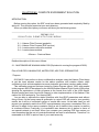
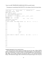
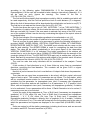
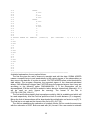
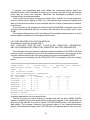
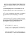
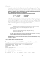
OCCAM 5.0. USER'S GUIDE
(O.Titov¹, V.Tesmer², J.Böhm³)
1 – Australian Surveying and Land Information Group (Canberra, Australia)
2 – German Geodetic Research Institute (Munich, Germany)
3 – Vienna Technical University (Vienna, Austria)
ABSTRACT
OCCAM 5.0 has new limits: 20 stations and 100 radiosources can be processed
simultaneously. The number of baselines under study is 190, correspondingly. The current
version of OCCAM supports IERS Conventions 2000. The ephemeride DE405/LE405
takes the place of DE403/LE403. To correct subdiurnal EOP variations two models can be
chosen: proposed by Ray (recommended by IERS Conventions 1996) and by Eanes
(IERS Conventions 2000) which takes into account many more tidal terms. A new leastsquares approach based on the Gauss-Markov model is available with the new version.
USER'S GUIDE MODIFICATIONS LOG
# WRITER
INSTITUTION
1.
2.
3.
4.
5.
6.
IAG, Madrid
18.03.1991
IAG, Madrid
13.01.1992
SK, Honefoss
17.12.1993
IAA, St.Petersburg
18.05.1997
SPbU, St.Petersburg
1999
SPbU, St.Petersburg
TU, Vienna
May 2001
5.0
DGFI, Munich
N. Zarraoa
N. Zarraoa
N. Zarraoa
O. Titov
O. Titov
O. Titov
J. Böhm
V. Tesmer
DATE
VERSION NUMBER
2.0
3.0
3.3
3.4
4.0
DISTRIBUTION LIST
Name
M. N. Kulkarni
B.R. Pettersen
V. Tesmer
Z. Malkin
M. Kudryashova
A. Mowlam
Qian Zhihan
V. Zharov
H.Schuh
Institute
Survey of India (Dehradun, India)
Norwegian Agriculture University (Norway)
German Geodetic Research Institute (Munich, Germany)
Institute of Applied Astronomy (Saint-Petersburg, Russia)
Saint-Petersburg University (Saint-Petersburg, Russia)
Melbourne University (Melbourne, Australia)
Shanghai Observatory (Shanghai, China)
Shternberg Astronomical Institute (Moscow, Russia)
Vienna Technical University (Vienna, Austria)
PREFACE
1. OCCAM V 5.0 is a Research and Development package for the analysis of geodetic
and geodynamics VLBI experiments. It is distributed freely.
2. The OCCAM Coordinator will be responsible for maintaining the configuration control
on the standard OCCAM. Modifications that prove their worth and usefulness may be
incorporated to the standard version and distributed to all users.
3. Presently the OCCAM Coordinator name and address is:
Oleg Titov
Australian Surveying and Landing Information Group (AUSLIG)
PO Box 2, Belconnen, Canberra, ACT 2616, Australia
Tel.: + 61 2 62014361
Fax: + 61 2 62014366
E-mail: [email protected]
4. Please, do not distribute the package OCCAM by yourself without informing the
OCCAM Coordinator. This formality will help the distribution of upgraded versions of the
package to all interested users.
2
5. If you find any part of this User's Guide difficult to understand, incomplete or in
disagreement with your experience as OCCAM user, please send your comments and
suggestions to the OCCAM coordinator preferably via electronic or standard mail.
6. If you find serious problems using the OCCAM package, we may provide some
assistance, only if you send to the OCCAM Coordinator a written report, as complete as
possible, on the problem found.
7. We strongly recommend that if you find any bug or error in the source code of
OCCAM, you send a report about it to the OCCAM Coordinator to distribute a corrected
version to all the users.
8. You may have implemented new modules or upgraded already existent ones in
OCCAM that could be useful for other users. If you want your changes to be definitely
implemented in the standard version of OCCAM, send the new source code with complete
information about the new features to the OCCAM Coordinator. Upgraded versions of
OCCAM will be periodically distributed to all users.
CONTENTS
PRELIMINARY INFORMATION
Introduction
Configure your computer to run OCCAM
What do I really need to process data
Running OCCAM V5.0
CHAPTER #1. COMPUTE MODEL AND CREATE STANDARD DATA FILES
1.1 - Automatic model computation
1.2 - Data handling
1.3 - Precession and nutation
1.4 - Station corrections and derivatives
1.5 - Geometric model
CHAPTER #2. COMPUTE EXPERIMENT SOLUTION
2.1 – Kalman Filter Process (geodetic)
2.2 – Kalman Filter Process (EOP service)
2.3 – Least squares collocation method
2.4 – Least squares method
CHAPTER #3. UTILITIES
3.1 - Extract information from OCCAM standard files
3.2 - Extract Obs-Calc files
APPENDIX A. Description of NGS data formats
APPENDIX B. Formats and examples of external and output files
APPENDIX C. Description of OCCAM internal files
3
PRELIMINARY INFORMATION
INTRODUCTION
The package OCCAM V 5.0 provides a useful tool to process VLBI sessions with an
Personal Computer (PC) running with WINDOWS (version 95 or higher). Complete tests
have been carried out with Pentium II/Pentium III based processors. Additionally, the
version 5.0 is in regular use with LINUX.
The software package OCCAM consists of several executable programs, which must
be used in strict order to get a solution of a VLBI session. There are some auxiliary
programs in the package, too. The executables can be started manually or automatically
via batch files. Please note that the batches work with WINDOWS only. Their use is not
supported by LINUX.
It is recommended to use powerful computers for data analysis because the modern
observational experiments include the tremendous number of observations.
This user's guide will concentrate on the use of OCCAM on a PC environment.
Since the previous OCCAM 4.0 version the following changes have been done
–
–
–
–
–
–
IERS Conventions 2000 replaced the IERS Conventions 1996;
Least squares method was added as an option to get a solution;
Troposphere gradients can be estimated optionally;
Reference station can be chosen manually;
Elevation cut off angle can be specified at the *.opt file;
OCCAM does not use virtual disks anymore
CONFIGURE YOUR COMPUTER TO RUN OCCAM
It is recommended to have at least 10 Mbytes free space on Hard Disk to contain the
program, data files and solution outputs. The executable code would need 4 Mbytes of
space.
Your computer must have as many Mbytes of RAM memory as available. But it is
possible to compile all FORTRAN files with advanced compiler (Lahey, Fortran Power
Station, etc.) to make use all available RAM memory.
The best configuration to keep the program in your computer is to separate the program
directory from the working directory where you process your data. If you have a comressed
Version of the OCCAM software, all files will be in the right path after the decomression. A
suitable configuration may read like this:
C:\OCCAM
C:\OCCAM\BAT
C:\OCCAM\SCR
C:\OCCAM\COMPILE
C:\OCCAM\EPHEM
C:\OCCAM\ATM
C:\OCCAM\WORK
Executable code of OCCAM 5.0
BATCH Files to run OCCAM Menu System
Screen files for the menu system
Source code of OCCAM
Ephemerides and EOP files
Atmospheric loading data
Working directory
4
C:\OCCAM\FIL
C:\OCCAM\DOC
Useful information
Documentation
These are the files that are installed into your work directory:
CHOOSE.COM
KVLBI.OPT
THERMAL.DEF
COLLOCAT.OPT
KVLBI_IE.OPT
OCCAM.SCR
EPHEM.DAT
LOADING.OCE
OCCAM.BAT
LSM.OPT
You will also need to have a catalog file (with extension .CAT) contains information
about positions of stations and radiosources and velocities of stations. The current version
includes a ITRF2000.CAT file as well. The file contains ITRF2000 catalog for station
coordinates and velocities and ICRF extension 1 for radiosources coordinates.
Pay attention that the disk C is used on default. OCCAM and data files to be stored into
the disk C. Corresponding paths are included in all *.BAT files. If you use another disk, the
*.BAT file must be updated for data analysis.
WHAT DO I REALLY NEED TO PROCESS DATA
1. INPUT DATA FILES FOR THE EXPERIMENT.
OCCAM uses VLBI data in NGS-Format. If your data is in any other format you must
change it to NGS before using OCCAM. NGS files can be downloaded from data servers
of the IVS, like ftp://cddisa.gsfc.nasa.gov/vlbi/ivsdata/ngs.
If you have NGS-Format data follow the instructions in Chapter #1.
2. NECESSARY FILES
When you install OCCAM several files are copied to your work directory. Some of them
are examples of the necessary files described below. Some other files may also be
necessary. It may be very useful for you to create similar files (e.g. own catalogs,
ephemerids tables, option files, etc.) according to your needs.
These are the files you need to run OCCAM:
A. CATALOG. Required from beginning to end. You should create your own catalog
containing the coordinates and velocities (if you wish to apply an a-priori velocity model) of
the stations and the celestial coordinates of the sources involved in the experiment. It would
be useful to create a global catalog with all the stations and sources you may need.
The installation of the OCCAM 5.0 provides you with the file ITRF2000.CAT as an
example. See Appendix B for a description. Any name is valid for this file.
B. EPHEMERIS TABLE. Required for ‘Precession and Nutation’ option in Model
Computation Menu (#1.2). You must create a file called EPHEM.DAT for your experiment.
This file should contain:
Earth Orientation Parameters (hereafter EOP): You can obtain this information from the
International
Earth
Rotation
Service
(IERS)
C04
series
from
IERS
(http://hpiers.obspm.fr/eop-pc). You will have to include EOP data not only for the
experiment's date but also for several days around. Nine or more data records should
provide a more precise interpolation. OCCAM 5.0 version makes use of the Lagrangian
interpolation scheme and can add subdiurnal EOP corrections as recommended by the
IERS.
5
Sun, Earth and Moon ephemerids: This information is available from DE/LE405 code in
accordance with IERS 2000 Conventions. It is advisable to include 5-6 days of data in your
table for a better interpolation. OCCAM requires an information with 0.5-day steps.
OCCAM can generate the EPHEM.DAT file for the experiment automatically. In order to
do that, you have to provide a complete ephemeride catalog for the year of the experiment
you want to run, and a similar file for EOP. The name of the files must be EPHEM.ye and
EOP.ye, where "ye" is the year of the experiment (99,00,01,...). They should be stored in
the ..\OCCAM\EPHEM subdirectory. A description of the files can be found in appendix B.
C. OCEAN LOADING DATA. Required for "Station Corrections and Derivatives" option
in the Model Computation Menu (#1.3). If you want to add corrections due to the ocean
loading effect, you must provide the amplitudes and phases of the main tidal components
at each station. The example file LOADING.OCE contains real data for several antennas.
The name of the file must be LOADING.OCE so you can simply add the information for
your antennas to the present file or update the existing information if better data is
available. The files are provided by Hans-George Scherneck via ftp service
(ftp://gere.oso.chalmers.se/pub/hgs/oload/olrs19_VLBI.blq). A close description of the
strategy to obtain the coefficients can be found at the Web address
http://www.oso.chalmers.se/~hgs. One version of the file is enclosed. See appendix B for a
detailed explanation of the file and its format.
D. THERMAL DEFORMATION DATA. Required for the "Station Corrections and
Derivatives" option in the Model Computation Menu (#1.3) and recommended by the IERS
Conventions. The description of the model used can be found in Haas et al,1999
http://www.dgfi.badw.de/dgfi/DOC/report71.pdf). The antenna dimensions information is
taken from the file THERMAL.DAT from the IVS Analysis Coordinator’s homepage
(http://miro.geod.uni-bonn.de/vlbi/IVS-AC). The initial mean temperature has been chosen
using some summarized experiences. If we did not have a reliable amount of data, the
value is equal to 999°C and no correction will be applied. The user can change it. A
description of the THERMAL.DEF file can be found in appendix B.
E. ATMOSPHERIC LOADING DATA. Also required for the "Station Corrections and
Derivatives" option in the Model Computation Menu (#1.3) and recommended by the IERS
Conventions. The data must be stored in a subdirectory ..\.OCCAM\ATM. Each station has
got an own time series of corrections, though a own [station_name].ATM file. The version
5.0 interpolates the quarter-daily corrections computed by Scherneck, which can be found
and downloaded on http://www.oso.chalmers.se/~hgs/apload.html. These data sets are
computed with the today’s probably most reliable approach. This approach additionally
needs the file ATMEAN97 which consists of ‘correction offsets’ due to a mean pressure for
each station (http://www.oso.chalmers.se/~hgs/apload.html). These are subtracted from the
corrections by the software. A description of the files is to be found in appendix B.
F. CONTROL FILES. All *.OPT files are required for running the solutions with the
Solution Computation Menu (Chapter #2). KVLBI.OPT is used for the "Kalman Filter
Process (Multibaseline)"(#2.1). KVLBI_IE.OPT is used for the "Kalman Filter Process
(Multibaseline)"(#2.2). COLLOCAT.OPT is used for the "Least Squares Collocation
Technique"(#2.3). .OPT is used for the "Least squares method (LSM)"(#2.4).A description
of these files is provided in Chapter #2.
G. To use some utilities you may need other files. You will find descriptions of those files
either in appendix B or the chapter referring to the utility itself.
H. There are other necessary files created by OCCAM like the OCCAM Standard Data
Files (SDF) or the clock model file. These are described in chapter #1 and appendix C.
6
RUNNING OCCAM V 5.0
Once you have configured your computer and installed the basic files into your hard disk,
you just have to enter "OCCAM" and your screen will look like this:
––––––––––––––––––––––––––––––––––––––––––––––––––––––––––––––––
OCCAM V 5.0
S Y S T EM M E N U
––––––––––––––––––––––––––––––––––––––––––––––––––––––––––––––––
1 - Compute Model and Create Standard Data Files
2 - Compute Experiment Solution
3 - Utilities
<Return> - Exit to DOS
––––––––––––––––––––––––––––––––––––––––––––––––––––––––––––––––
Detailed descriptions of the different options will follow. To select any item you only have
to enter the corresponding number.
========================================================
IMPORTANT!
Remember not to hit <RETURN> after the number, because the option is only used to quit
or go one menu back.
If your Menu present options like "1.2", you must only enter the last digit as selection. First
digit corresponds to the main menu option number. So, for "1.2" you only enter "2".
========================================================
The normal sequence of operations needed to process an experiment is the following:
A. Select Option 1 to get the Model Computation Menu (MCM).
B. From the MCM choose options #1.2, #1.3, #1.4 and #1.5 in this order. All four
options have to be completed. If you want to repeat any of them, the following ones have to
be repeated as well. With option #1.1 (Automatic mode) you make the complete chain.
C. Go back to the System Menu and select Option #2 to get the Solution Computation
Menu (SCM).
D. OCCAM 5.0 version supports Kalman filter, least squares method and least squares
collocation technique to get the solution.
CHAPTER #1.
COMPUTE MODEL AND CREATE STANDARD DATA FILES.
INTRODUCTION
7
When you enter option #1 in the System Menu your screen will look this way:
––––––––––––––––––––––––––––––––––––––––––––––––––––––––––––––––
OCCAM V 5.0
M O D EL COMPUTATION MENU
––––––––––––––––––––––––––––––––––––––––––––––––––––––––––––––––
1.1 - Automatic Model Computation
1.2 - Data Handling
1.3 - Precession and Nutation
1.4 - Station Corrections and Derivatives
1.5 - Geometric Model
<Return> - Previous Menu
––––––––––––––––––––––––––––––––––––––––––––––––––––––––––––––––
These options allow you to reformat your data set into OCCAM SDF, compute models
and corrections to generate theoreticals for the observables and compute partial
derivatives for the adjustment.
You can choose between the automatic model generation in option #1.1 or step by step
model generation using options from #1.2 to #1.5. Before running any of this options all the
previous ones must have been already completed.
More detailed descriptions of these options follow.
1.1 - AUTOMATIC MODEL COMPUTATION.
This option is equivalent to running options #1.2, #1.3, #1.4 and #1.5 in this order. Thus,
refer to the following items for explanations.
1.2 - DATA HANDLING (Equivalent to running the program DTAU0).
Files: DTAU.FOR, OCCAM_N.FI, DTAU1.FOR, LSM_OPT.FOR, OPT.FOR, ARC.FOR,
OPENING.FOR
* Purpose
This option reads the original VLBI data files for the experiment given in NGS format
and converts them into OCCAM SDF, which are used by the rest of the options in the
package. Detailed description of the NGS Format is provided in Appendix A.
The program reads global Ephemeris and EOP catalogs and creates the file
EPHEM.DAT specific for the experiment to be processed. The user can also create
EPHEM.DAT himself. The file format is described in Appendix B. The information needed
is described in the option #1.3 PRECESSION AND NUTATION.
The package OCCAM generates and uses several SDF. These are called SORTIM,
STATIM, BASTIM, BATCH, DICTIO and STACAT. All these files are created by this option.
A file called METEOR containing the meteorological data from the stations is also
generated but it is not used any more by the package.
8
This option creates the files with their final size. The rest of the options only add or read
information on them. SORTIM stores information regarding sources and time. One record
is reserved for each source-time combination. It contains the observation time tag (UTC),
the source observed and its coordinates, interpolated EOP, Ephemeris of Sun, Earth and
Moon, sidereal time, etc.
STATIM includes information regarding stations. It reserves one record for each pair
station-observation time. Station coordinates corrected for Earth Tides, Ocean Loading,
Pole Tide, etc. are stored here as well as tropospheric models, axis offsets and partial
derivatives with respect to source and station coordinates. Local meteorological data and
source coordinates (azimuth, hour angle and elevation) are also included here.
BASTIM has one record for each single scan (pair baseline-time). It contains the
observed and theoretical delays and rates, ionospheric corrections, etc.
STACAT is a catalog of the stations included in the experiment.
DICTIO is a directory of "where to look for" different items of data. For each baseline it
specifies in which record of BASTIM each scan is included.
These files are Direct Access files. Their contents can be read using #3.1 "Extract
information from OCCAM Standard Files".
BATCH is a list of the present baselines of. It also specifies which catalogue is used
and whose stations should be run.
METEOR is an ASCII file containing surface meteorological data and cable calibrations
extracted from the original Data File. It can be used to check if any station has no
meteorological data available.
A detailed description of all these files is found in appendix C.
In following steps the package generates other files that will be described when
necessary.
* How to use DATA HANDLING
When you select this option you are advised that any existent OCCAM SDF will be
erased. As the names of the files are fixed, erasing them at the beginning avoids errors in
the future.
The program will ask the user to provide some information:
A. Experiment Name (8 characters). It gives a key for the experiment that can be
followed when backing up files, etc. A name related to the Experiment's date and
type is a good choice (e.g. IRISA570).
B. Catalog to be used (12 characters). You must enter the name of the catalog for
Source and Station coordinates. See appendix B for a description of the format of
the catalog. An example of catalog is copied to your work directory when installing
OCCAM with the name ITRF2000.CAT
C. Data File Name (12 characters). The name of the NGS-Format data file must be
entered.
========================================================
If the program does not find any of these files, it repeats the request for the file name.
========================================================
If any source or station included on the data set is not available on the catalog the
program flags warning messages. It is recommended to quit and update the catalog before
continuing.
9
D. The next step asks you if OCCAM shall create the *.OPT files automatically. The
default is Y for yes, but have in mind that it is not necessarily the optimal choice for
each individual session. If you choose Y, the next options below (E, F, G) to be
answered more. If you choose N, there will be no more questions and you will follow
to step H.
E. The program shows a list of the existing stations and asks which of them is to be
taken as reference. If your input is not one of the observing stations, the first station
listed is chosen.
F. The following question ‘estimate atmosphere gradients ?’ is valid for the Kalman
filter approach only.
G. The following question ’24-hour or INTENISIVE 2-hour experiment? (24/02) specify
which type of session to be analyzed.
The package has some limits in the number of observations it can handle. Version 5.0 is
limited to 20 Stations, 100 Sources and 1000 different scans (observation to a single
source at the same time by two or more stations). If these limits are overflown then error
messages are displayed and the program aborts.
H. The program can generate automatically the file EPHEM.DAT used by the #1.3
option PRECESSION AND NUTATION. To do so the user has to provide the path to
search for the global ephemerides and EOP files. The pathway ..\OCCAM\EPHEM
is recommended. More details about EPHEM.DAT can be found in appendix B.
1.3 - PRECESSION AND NUTATION (equivalent to running the program PN).
Files: PN.FOR, EANES.FOR, VLPN.FOR, NUTATION.FOR, MHB.FOR, HERR_NUT.FOR,
ARC.FOR, OPENING.FOR, RAY.FOR, MATRIX.FOR, ROT.FOR
* Purpose
This option transforms between the J2000.0 Celestial Reference Frame for the quasars
to their apparent positions in the observation time.
EOP and Ephemeris data for Sun, Earth and Moon are read from a file called
EPHEM.DAT and interpolated to each observation’s epoch. See appendix B for a
complete description of the formats of the file. This information is stored on file SORTIM for
further use.
The information for EPHEM.DAT can be obtained in several ways:
Earth Orientation Parameters: IERS distributes EOP C04 yearly time series from IERS
Web site(http://hpiers.obspm.fr/eop-pc/).
Ephemeris: Global catalogs of ephemerides can provide barycentric Earth position and
velocity and Sun and Moon geocentric position and velocities. That info can be included
under the headers EARTD, SUND, MOOND. If global catalogs are available for the user,
the option #1.2 can be used to generate directly EPHEM.DAT, entering the path where
those files are. Their name has to be EPHEM.ye or EOP.ye, where “ye” means the year
(99, 00, 01, etc.). Check the formats of those files in appendix B.. DE405/LE405
ephemerides are used for OCCAM 5.0.
* How to use PRECESSION AND NUTATION
10
During the execution of this program, you can turn off several models that are applied in
this program. The following menu is displayed:
DEFAULT MODELS WILL BE APPLIED FOR:
A. - SHORT PERIOD UT1 VARIATIONS
B. - EFFECT OF OCEANIC TIDES ON UT1 AND POLAR MOTION
DO YOU WANT TO CHANGE THIS (Y, (N), Q TO QUIT)?
You can turn off any of them at this step. The default is applying them both.
The next step will be a more detailed question on the model for the effect of oceanic tides
on UT1 and polar motion (if model option B chosen before):
CHOOSE MODEL TO BE APPLIED FOR:
A. - RAY MODEL – IERS 96 CONVENTIONS
B. - EANES MODEL – IERS 2000 CONVENTIONS – (ON DEFAULT)
The default in OCCAM is B. Both options A and B use the Lagrangian interpolation
scheme for EOP, as recommended by the IERS.
The test calculations showed that for UT1-UTC there is a good agreement between
observational and model subdiurnal variations. For pole coordinates difference are larger
due to unknown reasons. Perhaps, there are strong non-tidal effects in pole motion.
Then the user will have to choose the a-priori nutation model:
A. - IAU 1980 NUT.MODEL ? (ON DEFAULT)
B. - HERRING MODEL ?
C. - MBH_2000 MODEL ?
Default is A, but the choice depends on the goal of the solution. The most precise model
should be MBH_2000.
The next option is to choose the Short Period UT1 variations to apply (if option A selected
in the very first step of this program):
FOR THE TIDAL UT1 VARIATIONS YOU CAN CHOOSE BETWEEN:
A. - IERS-STANDARDS (1989) (UT1–UT1R SHORT PERIOD < 35 DAYS)
B. - IERS-CONVENTIONS (1992) (UT1–UT1S SHORT AND LONG PERIODS)
SELECT YOUR PREFERENCE
For good interpolation of UT1 we need to subtract short-term variations with periods
less than 35 days. The default in OCCAM is A, because the updated model of the IERS
Conventions 1996 includes the terms that are already present on the EOP tables that are
standard in OCCAM. The bulletin B 1-days series (EOP1 code in EPHEM.DAT) has no
11
terms with period shorter than 35 days applied. Thus, after interpolation, option A is
applied to restore the terms in final UT1 time series.
Overall, there are three steps
1. Subtraction of short-term (< 35 days) terms
2. Interpolation
3. Restoration of short-term (<35 days) terms
==================================================================
IMPORTANT! Other sources for EOP may require a special use of the UT1 corrections
and/or interpolation methods that are not included in OCCAM 5.0. Before using any other
source for EOP, please read carefully its description and check which options in OCCAM
are best for using that data.
=================================================================
1.4 - STATION CORRECTIONS AND DERIVATIVES (equivalent to running the program
STATION).
Files: STATION.FOR, OCCAM_N.FI, CORREC.FOR, PARTIALS.FOR, TROPOSPH.FOR,
ATM_SCH.FOR, MATTEW.FOR, ARC.FOR, OPENING.FOR.
* Purpose
This program stores the following information on file STATIM.
A. Corrections to the catalog station coordinates due to earth tides
B. Further such corrections due to antenna deformations, ocean loading, atmospheric
loading and the secular pole tide (can be deselected).
C. Antenna axis offset contributions to delays and rates.
D. Troposphere models by A. Niell.
E. Local source coordinates (azimuth, elevation, hour angle)
F. Partial derivatives of the delay with respect to station, source coordinates, nutation
parameters and EOP.
The model for the solid earth tides used in OCCAM 5.0 is the model by Matthews and
Dehant (1999), as recommended by the IERS CONVENTIONS 2000, exception the part
for permanent tide correction. In accordance with conventional approach (different from
IERS official recommendations!) the part for permanent tide “restitution” has not been
activated. Thus OCCAM’s reference surface on the earth is the artificial surface as used by
almost all known space geodetic softwares. For further information, the user is referred to
MATTHEWS (1999) (http://www.dgfi.badw.de/dgfi/DOC/report71.pdf).
To apply the ocean loading corrections the program needs an external file with the
amplitudes and arguments of the main tidal components for the model. This file must be
called "LOADING.OCE" and when installing the package an example with real data for all
VLBI stations is copied into your work directory. In Appendix B you can find a description of
the format in case you need to update this information.
* How to use STATION CORRECTIONS AND DERIVATIVES
12
The program allows the user to select if any correction to station coordinates should be
neglected. By default all corrections are included, but the user can neglect up to four
effects:
BY DEFAULT ALL CORRECTIONS WILL BE ADDED TO THE DATA BASES. DO
YOU WANT TO CHANGE THIS?
Answering Yes, you will receive the following message:
THIS CORRECTIONS ARE APPLIED...
A. ANTENNA DEF. B. OCEAN LOAD. C. ATMOS. LOAD. D. POLE TIDE
SELECT THE CORRECTIONS YOU WANT TO NEGLECT
---And the user can select which of them to drop.
1.5 - GEOMETRIC MODEL (equivalent to running the program GEOMET).
Files: GEOMET.FOR, QUASAR1.FOR, SLOG.FOR, ARC.FOR, OPENING.FOR
* Purpose
This program computes the theoretical delays and delay rates for each observable
included in the original data file. It considers the geometrical configuration of antennas and
all relativistic effects. The information is stored on the file BASTIM.
* How to use GEOMETRIC MODEL
The program can use one of three available geometric models:
SELECT THE RELATIVISTIC MODEL TO BE APPLIED
A. – IERS - 1992 MODEL
B. – IERS - 1996 MODEL
C. – IAU - 1997 MODEL
Enter your selection ((A)/B/C) (Q to quit)’/)
The default model is A from IERS Conventions (1992), what differs from previous
OCCAM version. The user can also choose whether to apply Earth Gravity correction to
light propagation or not. Default option is to apply it. This option is not available for IAU1997 model. It always applies the Earth Gravity correction to light propagation that can not
be deselected.
Meanwhile, the choice of correct relativistic model is not a simple problem. Sergey
Klioner kindly prepared a short description on the topic (see below). If you use ITRF2000
system you will have to choose the option A (default). If you want to use the IAU-1997
option you will have to scale the coordinates of stations from ITRF catalogue.
13
The VLBI model can be symbolically written as
c * (t(2) – t(1)) = -k * (x(2) – x(1)) + additional terms.
Here c – the speed of light, t(1) – time epoch of arrival the wave front to site x(1), t(2) – time
epoch of arrival the wave front to site x(2), k – scaling factor.
The exact form of these additional terms depends also on the scaling you use for t(i) and
x(i). The possibilities for t(i).
1. use TCG
2. use TT
The possibilities for x(i)
A. use no additional scaling (that is, use directly the spatial coordinates of the
Geocentric Celestial Reference System as defined by the IAU). We call this
choice x^GRS(i)
B. use scaling x^ TT (i) = x ^ GRS ( i) * (1 − L(G ) , where L( G) = 6.969 * 10 −10 .
What we observe is actually the delay in terms of TT, so the choice between 1 and 2 is
clear: choice 2 should be used. Absolutely INDEPENDENT of the choice between 1 and
2, we have to choose between the possibilities A and B. The IAU in 1997 in Kyoto has
officially prohibited to use the scaled coordinates x^TT(i). So the "IAU" choice is A and the
"IAU approach" is 2A (2 for time, A for coordinates), IERS1992 is 1A (this is also
equivalent to 2B, that is the formula for 2B is absolutely the same as for 1A within the
required accuracy). Note that IERS1996 was wrong in all meanings (different and wrong
choices of scaling).
However, the ITRF2000 was decided to be represented by scaled coordinates x^TT(i)
(this is against the IAU resolutions, but it was decided by a ITRF meeting in November
2000). Therefore, it is expected that the new IERS Conventions will support both the IAU
choice 2A and the ITRF choice 2B with appropriate explanations.
14
CHAPTER #2. COMPUTE EXPERIMENT SOLUTION
INTRODUCTION
Before running this option, the SDF must have been generated and completely filled by
option #1. They must be present at your work directory.
When you select this option your screen will show you the following menu:
––––––––––––––––––––––––––––––––––––––––––––––––––––––––––––––––
OCCAM V 5.0
SOLUTION COMPUTATION MENU
––––––––––––––––––––––––––––––––––––––––––––––––––––––––––––––––:
2.1 – Kalman Filter Process (geodetic)
2.2 – Kalman Filter Process (EOP service)
2.3 – Least squares collocation method
2.4 – Least squares method
<Return> - Previous Menu
––––––––––––––––––––––––––––––––––––––––––––––––––––––––––––––––
Detailed description of this menu follows.
2.1 - MULTIBASELINE KALMAN ANALYSIS (Equivalent to running the program KVLBI).
Files: KVLBI.FOR, KALMAN.FOR, MATRIX.FOR, ARC.FOR, OPENING.FOR.
* Purpose
OCCAM 5.0 can perform a direct multibaseline analysis using the Kalman Filter theory
to get the least squares results for the station positions and nutation offsets, while
considering clock and atmospheric terms as stochastic processes (random walks model).
This estimation program has been tested by Nestor Zarraoa (about 1992) with respect
to the program SOLVE developed by the NASA/Goddard Space Flight Center VLBI group,
showing the equivalence of both programs at the formal error level of the VLBI results.
Similar results have been found with respect to other implementation of the Kalman Filter
method for VLBI analysis by Tom Herring (MIT).
You are able to estimate the station positions with fixed EOP parameters and without
fixing of them. At the former case all systematic in a priori EOP will move to your geodetic
results, but it will be a 'unificated' system of results with errors. At the latter case you will
prevent your geodetic results from EOP incompleteness using some constrained. But you
will have to apply for the same constrains (fixing a set of stations) from session to session
to a reference frame. Practically it is impossible case because set of station in frame of
one special network is not fixed. When you compare your resulting EOP time series you
must remember that the set of constrained stations are kept for all sessions. Therefore it is
reasonable to fix EOP in spite of loss of your result accuracy.
15
* How to use MULTIBASELINE KALMAN ANALYSIS (for geodetic tasks)
The program is controlled by file KVLBI.OPT file. An example of the file is shown below:
========================================================
SIGMA ADDED
.01
FACTOR ADDED
5. DWN-MAN-IGN D
(METERS)
TROPOSPHERIC MODEL: NIELL
NIELL 85.
YES NUTATION OFFSET
NO EARTH ORIENTATION PARAMETERS
NO ATMOPSPHERIC GRADIENTS
NO. STATIONS 3
V CONSTRNT __N_ECC __E_ECC __H_ECC
WETTZELL 0.0
N 0.00
ONSALA60 0.0
N 0.00
TRYSILNO 0.0
N 0.00
.066
-.018
2.823
CONSTRAINED DIRECTIONS 1
WETTZELL ONSALA60
A PRIORI PARAM. AND FORMAL ERRORS (M) (NO. ST. – 1) ∗ 6 + 1
0.0
1.
0.0
10.
0.0
10.
0.0
10.
0.0
10000.
0.0
.010
0.0
1.
0.0
10.
0.0
10.
0.0
10.
0.0
10000.
0.0
.010
0.0
1.
A PRIORI POWER SP. DENSITY (PS∗∗2/S) (NO. STAT. – 1) ∗ 6 + 1
0.1
0.0
0.0
0.0
1.0
0.0
0.1
0.0
0.0
0.0
1.0
0.0
0.1
========================================================
A detailed explanation of every option follows:
The first line gives the user a chance to reweight and edit the data. SIGMA ADDED
means a constant factor to add quadratically to the a-priori sigmas of the observables as
they come in the data file. It is given in meters. FACTOR ADDED refers to the threshold for
data editing. The program computes the expected sigma of the observed-calculated
delays. If the difference is bigger than FACTOR times the expected sigma, then it may act
16
according to the following option DWN-MAN-IGN: If D the observation will be
Downweighted; if M the user will be asked to take a decision interactively (Manually); if I it
will be used as such (Ignore the warning). The format of the line is
(12X,F8.4,12X,F8.4,12X,A1).
The 2nd and 3rd lines specify that troposphere model by Niell is available and which will
be used respectively. Also the 3rd line specifies a limit of zenith distance (Z, in degrees).
Below the limit all observations will be downloaded by multiplication on factor to sec(Z)**2.
The 2nd line is not read and the format of the 3rd is (A3, 4X, F3.0).
The 4th line allows the user to turn off ("NO NUTATION...") or on ("YES NUTATION...")
the estimation of nutation offsets. 5th line works the same way with the estimation of EOP.
Both are read with (A1) format. If the user wants to estimate only some of the EOP or only
one of the nutation offsets it can be done by constraining the sigma of the a-priori value as
is explained below.
The 6th line indicates if the troposphere gradients to be estimated or not. (A1)
The 7th line specifies the number of stations to be processed, in format (13X,I2).
There is one line for each station to be processed, in which the following information is
provided: NAME, ADDED SIGMA, VERTICAL CONSTRAIN, SIGMA OF CONSTRAIN,
ECCENTRICITIES (NORTH, EAST, UP). The NAME must coincide with the name on the
data file and catalogs. The ADDED SIGMA is used for reweighting the data from that
station. The value will be added quadratically to the a-priori sigma of the observable.
VERTICAL CONSTRAIN (Y or N) indicates if the height component of the stations will
remain fixed or not to the a-priori value. SIGMA OF CONSTRAIN limits the strength of the
constraint (default 0.001m). The ECCENTRICITIES apply only to mobile sites, and are the
North, East and Up component of the antenna with respect to the geodetic mark. All values
are in meters and the format is (A8,2X,F6.3,2X,A1,2X,F8.5,3F8.5).
The next line asks how many directions will be constrained in the analysis. Format
(23X,I3).
If the number of fixed directions is not 0, there follow as many lines as constrained
directions, specifying the fixed baseline. The constrain will be given 0.001 m sigma.
Format is (A8,1X,A8).
Next line is just a comment line, but it must be there. It helps to find where the parameter
count starts.
Then there are as many lines as parameters to be solved, with their a-priori value and
sigma of such a-priori. The number of parameters are as follows. The first station, which
will be considered master station for the coordinates (fixed) and clock (fixed), will only
contribute the first parameter, its tropospheric term (and, if necessary two troposphere
gradients). All the other stations will contribute 6 or 8 parameters: X, Y, Z position, clock
offset, rate and tropospheric term (and, if necessary two troposphere gradients). If nutation
is to be estimated, 2 more parameters will be there. If Earth Orientation is to be solved, 3
parameters more are to be included.
In brief, the order of the parameters is: Trop. of St.#1 (and, if necessary two troposphere
gradients); X,Y, Z, Clk. offset, Clk. rate, Trop. of St.#2 (and, if necessary two troposphere
gradients); ...; X, Y, Z, Clk. offset, Clk. rate, Trop. of St.#n (and, if necessary two
troposphere gradients); Nutation in obliquity, Nut. in longitude (if on); X wobble, Y wobble,
UT1-UTC corrections (if on). This order will be kept all over the program and is the order in
which the parameters and sigmas are displayed in the output files (KVLBI.RES, KVLBI,
etc).
Units are meters for all the station parameters, including clock terms, and arc-seconds
for nutation and EOP. Format of each line is (2F20.3).
17
If the user wants to constrain parameters to their a-priori value then the a-priori sigma
must be reduced accordingly. It permits that in practice some parameters are not
estimated but are fixed to their a priori values.
Then we have a new comment line, that permits to identify where the stochastic
characterization of the parameters start. All parameters are in principle considered
RANDOM WALK stochastic processes. So all of them can be given a rate of change with
time.
For a random walk, the sigma of the change of the value after a time interval DT, comes
as SQRT (PSD∗DT). PSD is the power spectral density of the WHITE NOISE associated
with the random walk. If PSD = 0 then the parameter is not allowed to change with time, so
it is considered a constant parameter. The user has to provide the PSD values for all the
parameters. The units required are picoseconds**2/second for all the station parameters
and arcseconds∗∗2/day for the nutation and orientation terms. There is one line for each
parameter with format (F10.3) in the same order as for the a-priori values and sigmas.
In general only troposphere (term and gradients) and clock offsets are considered
random walks, but orientation terms could be allowed a small rate of change, specially if
long experiments (more than 24 hours) are analyzed.
The final results of the program are stored in the file KVLBI.RES that can be directly
printed. Information about the evolution of the parameters with the successive filter
iterations can be either seen in files KVLBI.
The program displays the post-fit Chi-squared of the residuals during process, to check
that the options selected are in accordance with the data.
2.2 KALMAN FILTER PROCESS (for operational EOP service in frame of IVS).
(equivalent to running the program KVLBI_IE).
Files: KVLBI_IE.FOR, KALMAN.FOR, MATRIX.FOR, ARC.FOR, OPENING.FOR
It is a approach for operational EOP analysis, similar to 2.1. Station positions are fixed
using reference frame recommended by IERS.
The program is controlled by the file KVLBI_IE.OPT. An example of the file is shown
below:
===================================================================
SIGMA ADDED
.01
FACTOR ADDED
5. DWN-MAN-IGN D
(METERS)
TROPOSPHERIC MODEL: NIELL
NIELL 85.
YES NUTATION OFFSET
YES EARTH ORIENTATION PARAMETERS
NO STATION COORDINATES
YES ATMOPSPHERIC GRADIENTS
NO. STATIONS 3
V CONSTRNT __N_ECC __E_ECC __H_ECC
WETTZELL 0.0
N 0.00
ONSALA60 0.0
N 0.00
TRYSILNO 0.0
N 0.00
CONSTRAINED DIRECTIONS 0
A PRIORI PARAM. AND FORMAL ERRORS (M) (NO. ST. – 1) ∗ 5 + 3 + 5
0.0
1.
0.0
0.010
0.0
0.010
18
0.0
10000.
0.0
0.010
0.0
1.
0.0
0.010
0.0
0.010
0.0
10000.
0.0
0.010
0.0
1.
0.0
0.010
0.0
0.010
0.0
1.
0.0
1.
0.0
1.
0.0
1.
0.0
1.
A PRIORI POWER SP. DENSITY (PS∗∗2/S) (NO. STATIONS – 1) ∗ 5 + 3 + 5
0.1
0.001
0.001
1.0
0.0
0.1
0.001
0.001
1.0
0.0
0.1
0.001
0.001
0.0
0.0
0.0
0.0
0.0
========================================================
A detailed explanation of every option follows:
The first line gives the user a chance to reweight and edit the data. SIGMA ADDED
means a constant factor to add quadratically to the a-priori sigmas of the observables as
they come in the data file. It is given in meters. FACTOR ADDED refers to the threshold for
data editing. The program computes the expected sigma of the observed-calculated
delays. If the difference is bigger than FACTOR times the expected sigma, then it may act
according to the following option DWN-MAN-IGN: If D the observation will be
downweighted; if M the user will be asked to take a decision interactively (Manually); if I it
will be used as such (Ignore the warning). The format of the line is
(12X,F8.4,12X,F8.4,12X,A1).
The 2nd and 3rd lines specify that troposphere model by Niell is available and which will
be used respectively. Also the 3rd line specifies a limit of zenith distance (Z, in degrees).
Below the limit all observations will be downloaded by multiplication on factor to sec(Z)**2.
The 2nd line is not read and the format of the 3rd is (A3, 4X, F3.0).
The 4th line establishes the estimation of nutation offsets. 5th line works the same way
with the estimation of EOP. Both are read with (A1) format. If the user wants to estimate
19
only some of the EOP or only one of the nutation offsets it can be done by constraining the
sigma of the a-priori value as is explained below.
The 6th line indicates that station coordinates are not estimated. (A1)
The 7th line indicates if the troposphere gradients to be estimated or not. (A1)
The 8th line specifies the number of stations to be processed, in format (13X,I2).
There is one line for each station to be processed, in which the following information is
provided: NAME, ADDED SIGMA, VERTICAL CONSTRAIN, SIGMA OF CONSTRAIN,
ECCENTRICITIES (NORTH, EAST, UP). The NAME must coincide with the name on the
data file and catalogs. The ADDED SIGMA is used for reweighting the data from that
station. The value will be added quadratically to the a-priori sigma of the observable.
VERTICAL CONSTRAIN (Y or N) indicates if the height component of the stations will
remain fixed or not to the a-priori value. At the option it should be N always. SIGMA OF
CONSTRAIN limits the strength of the constraint (default 0.001 m).
The ECCENTRICITIES apply only to mobile sites, and are the North, East and Up
component of the antenna with respect to the geodetic mark. All values are in meters and
the format is (A8,2X,F6.3,2X, A1,2X,F8.5,3F8.5).
The next line asks how many directions will be constrained in the analysis. Format
(23X,I3). At the option should be 0 always.
Next line is just a comment line, but it must be there. It helps to find where the parameter
count starts. Then there are as many lines as parameters to be solved, with their a-priori
value and sigma of such a-priori. The number of parameters are as follows. The first
station, which will be considered master station for the coordinates (fixed) and clock
(fixed), will only contribute the first parameter, its tropospheric term (and, if necessary two
troposphere gradients). All the other stations will contribute 3 (or 5) parameters: clock
offset, rate and tropospheric term (and, if necessary two troposphere gradients). After 2
nutation parameters and 3 EOP need to be estimated.
In brief, the order of the parameters is:Trop. of St.#1; Clk. offset, Clk. rate, Trop. of St.#2
(and, if necessary two troposphere gradients); ...; Clk. offset, Clk. rate, Trop. of St.#n (and,
if necessary two troposphere gradients); Nutation in obliquity, Nut. in longitude; X-, Ywobbles, UT1-UTC corrections. This order will be kept all over the program and is the
order in which the parameters and sigmas are displayed in the output files (KVLBI.RES,
KVLBI).
Units are meters for all the station parameters, including clock terms, and arc-seconds
for nutation and EOP. Format of each line is (2F20.3).
If the user wants to constrain parameters to their a-priori value then the a-priori sigma
must be reduced accordingly. It permits that in practice some parameters are not
estimated but are fixed to their a-priori values.
Then we have a new comment line, that permits to identify where the stochastic
characterization of the parameters start. All parameters are in principle considered
RANDOM WALK stochastic processes. So all of them can be given a rate of change with
time.
For a random walk, the sigma of the change of the value after a time interval DT, comes
as SQRT (PSD∗DT). PSD is the power spectral density of the WHITE NOISE associated
with the random walk. If PSD=0 then the parameter is not allowed to change with time, so it
is considered a constant parameter. The user has to provide the PSD values for all the
parameters. The units required are arcseconds∗∗2/day for the nutation and orientation
terms. There is one line for each parameter with format (F10.3) in the same order as for the
a-priori values and sigmas.
20
In general only troposphere and clock offsets are considered random walks, but
orientation terms could be allowed a small rate of change, specially if long experiments
(more than 24 hours) are analyzed. Otherwise, the troposphere gradients can be
considered as a constant parameters.
If the control file has some errors (more stations than quoted, not enough parameter
lines for a-priori values, sigmas or PSD, etc.), the program flags a warning message and
aborts. Check that the number of lines coincides with the number of parameters or stations
in each block.
The final results of the program are stored in the file KVLBI.RES. Information about the
evolution of the parameters with the successive filter iterations can be either seen in files
KVLBI.
The program displays the post-fit chi-squared of the residuals during process, to check
that the options selected are in accordance with the data.
2.3 LEAST SQUARES COLLOCATION METHOD
(Equivalent to running the program COLL)
Files: COLL.FOR, COLL_ALL.FOR, C_EOP_0.FOR, DSINV.FOR, INFORM.FOR,
MK1.FOR, READING.FOR, SUBS1.FOR, SUBS2.FOR, ARC.FOR, OPENING.FOR
The collocation technique allows to estimate subdiurnal variations of the EOPs with time
resolution which corresponds to rate VLBI observation performance (one point per a few
minutes). Station positions are fixed using reference frame recommended by IERS.
The program is controlled by the file COLLOCAT.OPT. An example of the file is shown
below:
==================================================================
SIGMA ADDED
.01
FACTOR ADDED
15. DWN-MAN-IGN D (METERS)
TROPOSPHERIC MODEL: LANYI
DAVIS
MARINI
CHAO
NIELL 85.
YES NUTATION OFFSET
YES EARTH ORIENTATION PARAMETERS
NO ATMOSPHERIC GRADIENTS
NO. STATIONS 6
V CONSTRNT __N_ECC __E_ECC __H_ECC
WESTFORD 0.0
N 0.0
.0
.0
.0
GILCREEK 0.0
Y 0.0
.0
.0
.0
HARTRAO
0.0
N 0.0
.0
.0
.0
HOBART26 0.0
N 0.0
.0
.0
.0
ALGOPARK 0.0
N 0.0
.0
.0
.0
MATERA
0.0
N 0.0
.0
.0
.0
CONSTRAINED DIRECTIONS 1
WESTFORD MATERA
=====================================================================
A detailed explanation of every option follows:
The first line gives the user a chance to reweight and edit the data. SIGMA ADDED
means a constant factor to add quadratically to the a-priori sigmas of the observables as
they come in the data file. It is given in meters. FACTOR ADDED refers to the threshold for
data editing. The program computes the expected sigma of the observed-calculated
delays. If the difference is bigger than FACTOR times the expected sigma, then it may act
21
according to the following option DWN-MAN-IGN: If D the observation will be
downweighted; if M the user will be asked to take a decision interactively (Manually); if I it
will be used as such (Ignore the warning). The format of the line is
(12X,F8.4,12X,F8.4,12X,A1).
The 2nd and 3rd lines specify that troposphere model by Niell is available and which will
be used respectively. Also the 3rd line specifies a limit of zenith distance (Z, in degrees).
Below the limit all observations will be downloaded by multiplication on factor to sec(Z)**2.
The 2nd line is not read and the format of the 3rd is (A3, 4X, F3.0).
The 4th line establishes the estimation of nutation offsets. 5th line works the same way
with the estimation of EOP. Both are read with (A1) format.
The 6th line indicates if the troposphere gradients to be estimated or not. (A1)
The 7th line specifies the number of stations to be processed, in format (13X,I2).
There is one line for each station to be processed, in which the following information is
provided: NAME, ADDED SIGMA, VERTICAL CONSTRAIN, SIGMA OF CONSTRAIN,
ECCENTRICITIES (NORTH, EAST, UP). The NAME must coincide with the name on the
data file and catalogs. The ADDED SIGMA is used for reweighting the data from that
station. The value will be added quadratically to the a-priori sigma of the observable.
VERTICAL CONSTRAIN (Y or N) indicates if the height component of the stations will
remain fixed or not to the a-priori value. At the option it should be N always. SIGMA OF
CONSTRAIN limits the strength of the constraint (default 0.001 m).
The ECCENTRICITIES apply only to mobile sites, and are the North, East and Up
component of the antenna with respect to the geodetic mark. All values are in meters and
the format is (A8,2X,F6.3,2X, A1,2X,F8.5,3F8.5).
The next line asks how many directions will be constrained in the analysis. Format
(23X,I3).
If the number of fixed directions is not 0, there follow as many lines as constrained
directions, specifying the fixed baseline. The constraint will be given 0.001 m sigma.
Format is (A8,1X, A8).
Also you will be asked to input manually the following information:
- troposphere dispersion (in cm**2)
- clock dispersion (in cm**2)
- pole coordinates dispersion (in cm**2)
- UT1-UTC parameter dispersion (in cm**2)
- Pole parameters exponential coefficients
- UT1-UTC parameter exponential coefficient
- Phase for pole components
- Phase for UT1-UTC
The expected values follow the questions on the screen. Alternative choice can be made
on user’s feeling.
The amount of VLBI stations is limited to 8 ones for the option. At the first step the
observations are adjusted using weighted least squares method. The post-fit residuals are
calculated to fix the outliers which are downweighted at the next step.
The output files – UT1.DAT, X_EOP.DAT, Y_EOP.DAT contain the high-frequency
EOPs. Format is (F15.8,2X,F10.7) – for UT1.DAT; (F15.8, 2X, F9.6) – for others.
Output files are also: INFORM.DAT; SKO.DAT, EPS.DAT, ERP.DAT
The file INFORM.DAT contains a priori information used for the session analysis
22
The file SKO.DAT contains the calculated values: normalized chi-squared and weighted
root-mean squared - w.r.m.s – (in cm).
The file EPS.DAT contains post-fit residuals without separation on baselines. The order
numbers of VLBI sites are included here as well (in cm).
The file contains a daily estimates of five EOPs (as average values) for the session (all in arcsec).
2.4 LEAST SQUARES METHOD BASED ON THE GAUSS-MARKOV MODEL (LSM)
(Equivalent to running the program LSM).
Files: LSM.FOR, LSM_OPT.FOR, MNK.FOR, DSINV.FOR, OUTB.FOR, READOPT.FOR,
PREPARE.FOR, TIMSPLIT.FOR, ABAT2.FOR, ARC.FOR, OPENING.FOR
* Purpose
OCCAM 5.0 is able to do a classical least squares estimation with a large variety of
parameters that can be determined during the analysis. Principally, LSM is a two-step
approach with bad observations being downweighted after the first estimation step.
The basic number of parameters nr1 to be estimated for a 24 hour experiment is:
nr 1 = 1 + (nantenna − 1) * 7 + (2) + (3)
nantenna - the number of stations
i.e. for the reference station OCCAM 5.0 only solves for one troposphere (wet) zenith delay,
whereas for the other antennas, the station coordinates (x, y, z) and three clock parameters
(offset, rate and rate squared) are also adjusted. Additionally two nutation parameters and
three earth orientation parameters can be estimated once per 24 hour session.
Moreover LSM allows the estimation of further (auxiliary) parameters:
-) atmospheric gradients (offset and rate)
-) continuous piecewise linear functions:
∆L(t ) = ∆Loffset + ∆L rate,0 (t 1 − t 0 ) + ... + ∆L rate, n (t − t n )
This example shows a continuous piecewise linear function (plf) for the zenith delay,
i.e. OCCAM 5.0 solves for one offset and several rates. Plf's can also be used for
the clocks and gradients. Mind that auxiliary parameters for the clocks are always
estimated in addition to the quadratic function mentioned above.
-) discontinuous functions:
OCCAM 5.0 also offers the possibility to solve for other kinds of functions for the
auxiliary parameters (zenith delay, clock, gradients). For instance, there is the
chance to estimate offsets only for certain time intervals. More details can be found
in the description of the options file lsm.opt.
23
-) Constraints:
Constraints can be set for the offsets and rates of the auxiliary parameters. Those
constraints prevent the parameters from varying too much. Furthermore the setting
of the constraints might be necessary in order to avoid the singularity of the normal
equations. This is the case if parameters are estimated for a certain time interval
with no observations contributing to this parameter.
Constraints are set by specifiying the sigmas for observation equations:
∆L offset = 0 ± sigma
∆L rate = 0 ± sigma
for the offset
for the rate
Additionally the sigmas for the constraints can be further modified by setting an
'inverse fractional weight' ifw of the constraints. The reason for this option is that
there is a difference whether you set a constraint for a parameter with 300 or 100
observations contributing to it. In other words, the more observations you have the
smaller must be the sigma to have an equally powerful constraint.
Example:
300 observations contributing to a parameter (time interval: 2 hours)
sigma (random walk) is set to 20 mm/sqrt(h) in the options file
ifw is set to 10
variance = (20**2)/2 [mm**2/h**2] = 200 [mm**2/h**2]
variance = 200 / 300 * 10
So, the sigma 2.58 [mm/h] is used for the observation equation. If we only
had 100 observations the sigma would be 4.47 [mm/h].
Nevertheless, if you are not sure about this option, just set the ifw to 999. By doing
so, no ifw is applied.
* How to use the LEAST SQUARES METHOD
The program is controlled by the file LSM.OPT. An example of the file is shown below:
========================================================
SIGMA ADDED 0.010
FACTOR ADDED
5.00 DWN-MAN-IGN D
TROPOSPHERIC MODEL: NIELL
NIELL
CUTOFF ELEVATION: 10.0
NO
DOWNWEIGHTING FOR LOW ELEVATIONS: COSZ
COSZ**2
20.0 COSZ**2
YES NUTATION OFFSET
NO
EARTH ORIENTATION PARAMETERS
NO
FREE SOLUTION
NO. STATIONS 5
V N E CONSTRNT __N_ECC __E_ECC __H_ECC
24
KOKEE
0.000 N N N
0.00000
0.000
0.000
0.000
GILCREEK
0.000 N N N
0.00000
0.000
0.000
0.000
NRAO20
0.000 N N N
0.00000
0.000
0.000
0.000
WETTZELL
0.000 N N N
0.00000
0.000
0.000
0.000
FORTLEZA
0.000 N N N
0.00000
0.000
0.000
0.000
CONSTRAINED DIRECTIONS
1
WETTZELL FORTLEZA
----------------------------------------------------------AUXILIARY PARAMETERS
TIME INT.
ZD
ZDR
ZRS
CO
CR
CRS
GR
GRR
KOKEE
99.99 2.00 0.00 0.00 0.00 0.00 12.00 0.00
GILCREEK
99.99 2.00 0.00 99.99 1.00 99.99 12.00 0.00
NRAO20
2.00 2.00 0.00 99.99 1.00 99.99 12.00 0.00
WETTZELL
99.99 2.00 0.00 1.00 1.00 1.00 12.00 0.00
FORTLEZA
99.99 2.00 0.00 99.99 1.00 99.99 12.00 0.00
PIECEWISE LINEAR FUNCTIONS AND CONSTRAINTS
INVERSE FRACTIONAL WEIGHT OF CONSTRAINTS: 999
#RATES
RW ZDR PL
RW CLR PL
RW GRR PL
MM/SQRT(H)
MM/SQRT(H)
MM/SQRT(H)
KOKEE
15.000 Y
0.000 N
0.000 N
GILCREEK
15.000 Y
20.000 Y
0.000 N
NRAO20
15.000 N
20.000 Y
0.000 N
WETTZELL
15.000 Y
20.000 N
0.000 N
FORTLEZA
15.000 Y
20.000 Y
0.000 N
#OFFSETS
SIG ZDO EX
SIG CLO EX
SIG GRO EX
MM
MM
MM
KOKEE
0.000 N
0.000 N
0.500 N
GILCREEK
0.000 N
0.000 N
0.500 N
NRAO20
0.000 N
0.000 N
0.500 N
WETTZELL
0.000 N
0.000 N
0.500 N
FORTLEZA
0.000 N
0.000 N
0.500 N
========================================================
A detailed explanation of every option follows:
The first line gives the user a chance to reweight and edit the data. SIGMA ADDED means
that a constant number is added quadratically to the apriori sigmas of the observables as
they defined in the (ngs-) data file. It is given in meters. FACTOR ADDED refers to the
threshold for the editing of observations. The smaller this factor is, the more observations
are downweighted. The following criterion is used for the downweighting of the observation
i:
(v(i)**2)/sqrt(cofactor(i)) > factor
v(i) is the residual of the observation, and cofactor(i) is the cofactor aposteriori of the
residual.
The format of the line is (12X,F8.4,12X,F8.4,12X,A1).
The second and third lines specify which troposphere models are available and which will
be used respectively. Presently, the only option is the Niell mapping function (A3). Mind that
with OCCAM 5.0 (LSM) the dry zenith delay is calculated apriori and the wet zenith delay is
estimated by the least squares analysis.
25
The fourth line specifies the cutoff elevation angle. The format is (18X,F4.1). The fifth line
gives the user the chance to downweight low obervations (A1). The next line is then
intended to provide the elevation angle from which downweighting should be started and
the way of downweighting itself. (F4.1,2X,A7)
The next two lines allow the user to decide whether nutation and earth orientation
parameters should be solved for. Both are read with (A1) format. Mind that presently only
one set of nutation and/or eop parameters can be estimated for one 24 hour experiment.
The next line is intended to specify whether a free network solution should be estimated.
This option does not work yet. (A1)
The next line specifies the number of stations to be processed. The format that is used is
(13X,I2).
There is one line for each station to be processed, in which the following information is
provided: NAME, ADDED SIGMA, CONSTRAINT (VERTICAL, NORTH, EAST), SIGMA
OF VERTICAL CONSTRAINT, ECCENTRICITIES (NORTH, EAST, UP). The NAME must
coincide with the name in the data file and catalogs. The ADDED SIGMA is used for
reweighting the data from that particular station. This value will be added quadratically to
the apriori sigma of the observable. VERTICAL CONSTRAINT (Y or N) indicates if the
height component of the stations will remain fixed or not to the apriori value. The NORTH
and EAST CONSTRAINTS do not work yet. The SIGMA OF VERTICAL CONSTRAINT
limits the strength of the vertical constraint (default 0.001m). The ECCENTRICITIES apply
only to mobile sites, and are the North, East and Up component of the antenna with respect
to the geodetic mark. All values are in meters and the format is
(A8,2X,F6.3,2X,3(A1,2X),F8.5,3F8.5).
The next line asks how many directions will be constrained in the analysis. Format (23X,I3).
If the number of fixed directions is not 0, there follow as many lines as constrained
directions, specifying the fixed baseline. Format is (A8,1X,A8).
Hint: If all station coordinates should be fixed to their apriori values all directions and all
heights have to be constrained.
In the next paragraph the time intervals for the estimation of the the auxiliary parameters
have to be set. Mind that there is no estimation of clock parameters for the first (reference)
station. If you want to solve for a piecewise linear function plf you have to set one offset for
the whole experiment (24.00 or just take 99.99) and additionally the time intervals for the
rates have to be specified (e.g. 2.00 for a two hours' time interval).
The lsm.opt file above shows some examples for the parametrization:
-) plf for the zenith delay at KOKEE e.g. (two hours time interval)
-) one-hour discontinuous quadratic functions for the clock at WETTZELL
-) two-hours discontinuous functions for the zenith delay at NRAO20
-) twelve-hours offsets for the gradients for all stations
In particular the items are: NAME, ZENITH DELAY OFFSET, ZENITH DELAY RATE,
ZENITH DELAY RATE SQUARED, CLOCK OFFSET, CLOCK RATE, CLOCK RATE
SQUARED, GRADIENT OFFSET, GRADIENT RATE. The format is (A8,3X,8(F5.2,1X)).
The inverse fractional weight of constraints should be set to 999 by default. By using it the
sigmas of the constraints for the plf's can be adapted to the numbers of observations within
a certain time interval. (42X,I3)
The next paragraph specifies the constraints for the rates of the plf's. Mind that plf's have to
be marked with 'Y' in order to distinguish them from discontinuous functions. The units of
the constraints (sigmas) are comparable to those of random walk parameters (mm/sqrt(h)).
The items are: NAME, ZENITH DELAY RATE, PLF (Y or N), CLOCK RATE, PLF,
GRADIENT RATE, PLF. (A8,3(3X,F7.3,2X,A1))
26
The last paragraph contains information for the offsets of the auxiliary parameters. Do not
use an offset constraint for the (wet) zenith delay, but do use a constraint for the gradient
offset. If the sigma for the offset is set to 0.000 no constraint will be applied
The items are: NAME, ZENITH DELAY OFFSET, EX, CLOCK OFFSET, EX, GRADIENT
OFFSET, EX. (A8,3(3X,F7.3,2X,A1)) The symbol EX means that external information (e.g.
zenith delays by GPS) can be introduced but this options does not work with this version.
27
CHAPTER #3. UTILITIES
INTRODUCTION
In this option we have included some programs that usually are not needed during
standard processing but that may be useful in certain cases.
With this option, the user will see the following menu:
:––––––––––––––––––––––––––––––––––––––––––––––––––––––––––––––––
:
OCCAM V 5.0
U T I L I T I ES M E N U
:––––––––––––––––––––––––––––––––––––––––––––––––––––––––––––––––
:
:
3.1 - Extract information from OCCAM Standard Files
:
3.2 - Extract Obs-Calc Files
:
<Return> - Previous Menu
:
:––––––––––––––––––––––––––––––––––––––––––––––––––––––––––––––––
3.1. EXTRACT INFORMATION FROM OCCAM STANDARD FILES (DUMPTHEO)
Files: DUMPTHEO.FOR, OPENING.FOR, ARC.FOR
This options allows to extract information from OCCAM SDF. Data can be extracted
from BASTIM, STATIM, SORTIM and STACAT. Information from BASTIM can be extracted
by record number, by source, by station or the whole file. There are interactive menus to
select how to extract the data for all files. Information from STATIM can be extracted from
the whole file, by source or by record number. Information from SORTIM is extracted by
record number. If file STACAT is to be read, the full file is processed. File "OUTPUT.XTC"
contains the extracted information.
3.2. EXTRACT OBS-CALC FILES (Code EXTRACT)
Files: EXTRACT.FOR, OPENING.FOR, ARC.FOR
This option reads the SDF and generates a series of outputs with several information:
OUTPUT.OMC includes the Obs-Calc values plus the tropospheric calibrations (DAVIS
model). It writes the station names, source name, year, day of year, hour, minute, integer
second, observed minus computed delay, atmospheric correction for station 1 and 2. The
format is (1X,A8,1X,A8,2X,A8,2X,I4,1X,I3,1X,3I2,2X, 3D22.16).
OUTPUT.THE includes the theoretical delays. The variables written are: record number,
station names, source name, year, day of year, hour, minute, second, theoretical without
atmospheric model and theoretical with atmospheric model. The format used is:
(I3,A8,1X,A8,2X,A8,2X,I4,1X,I3,1X,3I2,2X,2D22.16).
OUTPUT.PAR lists the partial derivatives respect to all parameters. It writes the station
names, source name, year, day of year and hour, minute, second, observed minus
computed delay and the partial derivatives with respect to X, Y, Z (1st station), X, Y, Z (2nd
station), atmospheric parameter (1st and 2nd station), RA and Declination of source,
28
nutation obliquity and longitude. The format is: (A8,1X,A8,2X,A8,2X,I4,1X,I3,1X,3I2,2X,
13D15.8)
These files are useful for plotting, comparison or debugging.
APPENDIX A.
DESCRIPTION OF THE NGS VLBI FORMAT
NGS VLBI DATA FORMAT
1. Site cards
Col. 1- 8: Site name
Col. 11-25: Site X component (m)
Col. 26-40: Site Y component (m)
Col. 41-55: Site Z component (m)
Col. 57-60: Axis type
Col. 61-70: Axis offset
End of site cards is indicated by $END
2. Source cards
Col. 1- 8: Source name
Col. 11-28: Right ascension HH MM SS.SSSSSSSSS
Col. 31-48: Declination sDD MM SS.SSSSSSSSS
End of source cards is indicated by $END
3. Auxiliary parameters
Col. 1-20: Reference frequency
Col. 21-30: Group delay ambiguity spacing
Col. 32-33: Delay type (GR or PH)
Col. 35-36: Delay rate type (GR or PH)
End of this card is indicated by $END
4. Data cards
Card # 1
Col. 1-18: Names of site #1 and site #2
Col. 21-28: Source name
Col. 30-60: Time YYYY MM DD HH MM SS.SSSSSSSSSSS
Col. 61-70: Run identification code
Col. 71-78: Sequence number
Col. 79-80: 01
Card # 2
Col. 1-20: Observed delay (ns)
Col. 21-30: Formal error of observed delay (ns)
Col. 31-50: Observed delay rate (ps/sec)
Col. 51-60: Formal error of observed delay rate (ps/sec)
Col. 61-62: Data quality flag (0 means good data)
29
Col. 64-68: Delay and delay rate type
Col. 69-69: I if ionospheric calibration applied
Col. 70-70: C if cable calibration applied
Col. 71-78: Sequence number
Col. 79-80: 02
Card # 3
Col. 1-20: Correlation coefficient and formal error
Col. 21-40: Fringe amplitude and formal error (J)
Col. 41-70: Total fringe phase and formal error (rad)
Col. 71-78: Sequence number
Col. 79-80: 03
Card # 4
Col. 1-15: System temperature at site 1 and formal error (K)
Col. 16-30: System temperature at site 2 and formal error (K)
Col. 31-45: Antenna temp. at site 1 and formal error (K)
Col. 46-60: Antenna temp. at site 2 and formal error (K)
Col. 71-78: Sequence number
Col. 79-80: 04
Card # 5
Col. 1-20: Cable cal. correction for sites 1 and 2 (ns)
Col. 21-40: WVR parameter at site 1 and formal error (ns)
Col. 41-60: WVR parameter at site 2 and formal error (ns)
Col. 62-64: WVR parameter definition code at sites 1 and 2:
0.- parameter is zenith path delay
1.- parameter is path delay along line of sight
Col. 71-78: Sequence number
Col. 79-80: 05
Card # 6
Col. 1-20: Ambient atmosph. temperature at sites 1 and 2 (C)
Col. 21-40: Ambient barometric pressure at sites 1 and 2 (mb)
Col. 41-60: Atmospheric humidity parameter at sites 1 and 2
Col. 62-64: Humidity parameter definition at sites 1 and 2
0.- Relative humidity (%)
1.- Dew point (C)
2.- Wet bulb temperature (C)
Col. 71-78: Sequence number
Col. 79-80: 06
Card # 7
Col. 1-10: Time difference between reference epoch and the
start of observation (sec)
Col. 11-20: Duration of observation (sec)
Col. 21-30: A priori UTC offset at site 1 (sec)
Col. 31-50: Observation frequency (MHz)
Col. 51-60: Group delay ambiguity (ns)
30
Col. 71-78: Sequence number
Col. 79-80: 07
Card # 8
Col. 1-20: Ionospheric delay (ns)
Col. 21-30: Formal error of ionospheric delay (ns)
Col. 31-50: Ionospheric delay rate (ps/sec)
Col. 51-60: Formal error of ionospheric delay rate (ps/sec)
Col. 71-78: Sequence number
Col. 79-80: 08
31
APPENDIX B.
FORMATS AND EXAMPLES OF EXTERNAL FILES USED IN OCCAM
1. CATALOG. File name - any
First two columns determine the record code (RC).
RC = TC (terrestrial coordinates)
Col. 1- 2: Record code
Col. 4-11: Station name
Col. 12-28: X component (m)
Col. 29-43: Y component (m)
Col. 44-58: Z component (m)
Col. 60-63: Axis type. Valid types are:
AZEL.- Azimuth-elevation mounting
EQUA.- Equatorial mounting
X-Y1.- X-Y mounting North-South
X-Y2.- X-Y mounting East-West
Col. 64-73: Axis offset (m)
RC = TV (terrestrial velocities)
Col. 1- 2: Record code
Col. 4-11: Station name
Col. 12-19: X velocity (m/year)
Col. 20-27: Y velocity (m/year)
Col. 28-35: Z velocity (m/year)
RC = CC (celestial coordinates)
Col. 1- 2: Record code
Col. 4-11: Source name
Col. 13-27: Right ascension
HH MM ss.sssssss
Col. 32-47: Declination
sDD MM ss.sssss
Col. 50-57 Deviation in right ascension ss.sssssss
Col. 60-66 Deviation in declination
ss.ssssss
Source coordinates must be provided in J2000.0 reference frame
RC = HH
Col. 1- 2: Record code
Col. 4-70: Comments
RC = EP (epoch of the terrestrial coordinates/velocities)
Col. 1- 2: Record code
Col. 4- 9: Epoch (years)
2. EPHEMERIS FILE. File name.- EPHEM.DAT
First four columns determine the record code (RC).
32
RC = EOP1 or (Earth orientation parameters)
Col. 1- 4: Record code
Col. 7-13: Modified Julian date of the data
Col. 15-22: X wobble (arcsec)
Col. 23-30: Y wobble (arcsec)
Col. 33-41: UT1–UTC (sec)
Col. 44-45: TAI–UTC (integer number of seconds)
Col. 47-53: Nutation angle Dpsi (arcsec)
Col. 55-61: Nutation angle Deps (arcsec)
RC = MOOND (Moon ephemeris position and velocity)
Col. 1- 5: Record code
Col. 6- 13: Modified Julian date of data
Col. 14-157: X, Y, Z geocentric coordinates, X, Y, Z velocities
RC = EARTD
Col. 1- 5: Record code
Col. 6- 13: Modified Julian date of data
Col. 14-157: X, Y, Z barycentric coordinates, X, Y, Z velocities
RC = SUND
Col. 1- 5: Record code
Col. 6- 13: Modified Julian date of data
Col. 14-157: X, Y, Z geocentric coordinates, X, Y, Z velocities
The program assumes that the tables are given in UTC time for interpolation.
If you generate EPHEM.DAT automatically, you need global files for ephemerids and
EOP.
The ephemerids file for one year must be called EPHEM.ye, and it is convenient that it
overlaps a little with the previous and next year. Each record must contain all the
information for each epoch in free format. The variables are:
Record number; Epoch; Earth barycentric coordinates X,Y,Z, velocities X,Y,Z; Sun
geocentric coordinates X,Y,Z and velocities X,Y,Z; Moon geocentric coordinates X,Y,Z and
velocities X,Y,Z.
The EOP file for one year must correspond to the EOP1 series in the current
implementation of OCCAM and the format is free in the following order:
Epoch (MJD), X wobble, Y wobble, UT1–UTC, UT1–TAI
3. OCEAN LOADING DATA. File name – LOADING.OCE
The data is organized in blocks. One block for each station. Each block contains:
Record #1: Station name from column 1 to 8
Record #2: Amplitude of radial displacement for each component. 7 characters per
value (m).
Record #3: Amplitude of horizontal north-south displacement for each component.
33
7 characters per value (m).
Record #4: Amplitude of horizontal east-west displacement for each component.
7 characters per value (m).
Record #5: Phase of radial displacement for each component. 7 characters per
value (Deg).
Record #6: Phase of horizontal north-south displacement for each component.
7 characters per value (Deg).
Record #7: Phase of horizontal east-west displacement for each component.
7 characters per value (Deg).
The tidal components are indexed in the following order:
M2, S2, N2, K2, K1, O1, P1, Q1, MF, MM, SSA
Example of block. Only nine components shown but can be up to 11.
ONSALA60
R, PHR, TNS, PHNS, TEW, PHEW
0.384 0.091 0.084 0.019 0.224 0.120 0.071 0.003 0.084
0.058 0.027 0.021 0.008 0.032 0.017 0.009 0.004 0.007
0.124 0.034 0.031 0.009 0.042 0.041 0.015 0.006 0.018
-56.0 -46.1 -90.7 -34.4 -44.5 -123.2 -49.6 178.4
14.9
84.2 131.3
77.7 103.9
17.2 -55.0
25.2 -165.0 173.3
75.4
97.6
40.8
94.8 119.0
25.4
98.7 -14.1 -177.0
4. ATMOSPHERIC LOADING CORRECTION DATA.
File names: [station_name].ATM and ATMEAN97
These files have to be stored in the /ATM directory.
Each line of the *.ATM files, which contain the corrections for one station include the
following:
- Time of correction (mjd, four epoches per day)
corrections up, east, north [m]
Format of the lines in ATMEAN97, which contains corrections due to average pressure on
sites. It is subtracted from the correction to avoid offsets:
- eight character station name,
correction-offsets up, east, north [m]
5. THERMAL DEFORMATION CONTROL FILE. File name – THERMAL.DEF
The file THERMAL.DEF contains mainly the info from the file titled ‘thermal.dat’ from the
homepage of IVS Analysis Coordinator (A. Nothnagel) homepage (http://miro.geod.unibonn.de/vlbi/IVS-AC). Its format is:
The data is organized in blocks. Each block contains two lines:
line 1:
- eight character station name
line 2 (f9.5,f6.1,1x,f11.6,4(f6.1),i6,f6.1):
- gf [1/°C]
(expansion coefficient for foundation)
34
(height of concrete foundation)
(expansion coefficient for antenna)
(height of antenna pillar)
(height of vertex)
(height of subreflector)
(height of declination shaft)
(10 => factor for hs is 0.9 (for prime focus antennas only),
20 => factor for hs is 1.8)
- reference temperature [°C] (The usual reference temperature used for designing
and constructing buildings is 20°C. In this
approach, mean temperatures at the sites are used
for not generating offsets to the coordinates)
-
hf [m]
ga [1/°C]
hp [m]
hv [m]
hs [m]
hd [m]
ifo
35
APPENDIX C
DESCRIPTION OF OCCAM INTERNAL FILES
1. SORTIM (19)
Direct access file with record length of 752 bytes
1- 4 Dummy integer. On first record, total number of records
5- 12 Source name (Character*8)
13- 28 Right ascension and declination at 2000.0 (Real*8)
29- 40 Modif. Julian date and fraction of day in radians (Integer*4 and Real*8)
41- 48 Integer number of seconds between UTC and TAI (Real*8)
49-168 Apparent RA and Dec, and geocentric source direction unit vector (3) for one
second before, one after and at the observation time. All Real*8.
169-240 Earth barycentric coordinates (X,Y,Z) one second before, after and at the
observation time. Real*8.
241-312 Earth barycentric velocity (X,Y,Z) one second before, after and at the
observation time. Real*8.
313-384 Earth barycentric acceleration (X,Y,Z) one second before, after and at the
observation time. Real*8
385-432 Greenwich sidereal time and hour angle one second before, one after and at
the observation time. Real*8.
433-440 Earth Rotation velocity. Real*8
441-488 X wobble and Y wobble one second before, one after and at the
observation time.
489-560 Moon X,Y,Z geocentric coordinates one second before, one after and at the
observation time. Real*8
561-632 Geocentric sun coordinates (X,Y,Z) one second before, one after and at the
observation time. Real*8.
633-680 Partial derivatives of the source direction unit vector with respect to nutation
obliquity (3) and longitude (3). All Real*8.
681-752 Final matrix of precession and nutation (nine components, all Real*8).
2. STATIM (18)
Direct access file with a record length of 480 bytes.
1- 4 Dummy integer. Total number of records on first one.
5- 8 Record number for this station in file STACAT
9- 12 Record number of this observation in SORTIM
13- 40 Temperature, Pressure, Humidity and humidity factor. All Real*8. Last one
integer.
41- 48 Cable calibration. Real *8.
49-120 Station coordinates (X,Y,Z) one second before, one after and at the
observation time. Real*8
121-192 Station Coordinates (Longitude, latitude, height) one second before, one after
36
and at the observation time.
193-264 Zenith distance, hour angle and local sidereal time one second before, one
after and at the observation time.
265-280 Zenith tropospheric path delay "dry" and "wet".
281-312 Tropospheric mapping functions or corrections for delays and rates. Models Niell
(2 values).
313-328 Axis offset corrections (delay and rate).
329-408 Partial derivatives with respect to Z, X, Y, RA, Dec for delay and rate.
409-424 Partial derivatives with respect to the nutation offsets (obliquity and
longitude). Real*8
425-448 Partial derivatives with respect to the EOP (X,Y, UT1–UTC). Real*8
449-456 Thermal deformation of antenna. Real*8
457-464 Source azimuth. Real*8
465-480 Partial derivatives with respect to troposphere gradients. Real*8
3. BASTIM (17)
Direct access file with a record length of 144 bytes.
1- 4 Dummy integer. Total number of records in first one.
5- 8 Record number of the observation in file SORTIM
9- 16 Record number of the observation for station on STATIM
17- 48 Observed delay and rate with formal errors.
49- 80 Ionospheric correction for delay and rate and errors
81-104 Theoretical delay one second before, one after and at the observation time.
105-128 Theoretical rate one second before, one after and at the observation time.
129-136 Ambiguity correction term
4. DICTIO (21)
Direct access file with a record length of 2128 bytes
Each record represents one baseline, and it contains the list of record numbers in
BASTIM in which there is data of that baseline. An ambiguity correction term for the
baseline is also stored.
5. STACAT (20)
Direct access file with a record length of 128 bytes
1- 4 Dummy integer. Total number of stations on first record.
5- 12 Station name. (Character*8)
13- 36 Station a priori coordinates (X,Y,Z). Real*8
37- 44 Epoch for the a-priori coordinates. Real*8
45- 68 A-priori velocity of the station (X,Y,Z). Real*8
69- 72 Mounting type
37
73- 88 Axis offsets
89-112 Longitude, latitude and height
113-120 Geocentric radius of station
121-128 Equatorial component of station vector.
6. BATCH
ASCII file with the list of the involved baselines
7. METEOR
ASCII file with the meteorological data and cable calibration extracted from NGS-format
input file.
8. CLOCK BREAKS MODEL. Filename BREAKS.RES
Each record contains information about one single clock break but the Kalman Filter
program only reads columns 1 to 3. The third column information is not use now. The format
is (I3,2x,I3)
Col 1- 3: Station Code number
Col 5- 8: Time Code number
Col 11-14: Clock break type:
+1 .- Clock offset jump
-1 .- Clock rate variation
Example of file:
4 55 -1.0
1 63 -1.0
38