1
esys-Escript User’s Guide:
Solving Partial Differential Equations
with Escript and Finley
Release - development
(r5751)
Lutz Gross et al. (Editor)
July 15, 2015
Centre for Geoscience Computing (GeoComp)
School of Earth Sciences
The University of Queensland
Brisbane, Australia
Copyright (c) 2003-2015 by The University of Queensland
http://www.uq.edu.au
Primary Business: Queensland, Australia
Licensed under the Open Software License version 3.0
http://www.opensource.org/licenses/osl-3.0.php
Development until 2012 by Earth Systems Science Computational Center (ESSCC)
Development 2012-2013 by School of Earth Sciences
Development from 2014 by Centre for Geoscience Computing (GeoComp)
This work is supported by the AuScope National Collaborative Research Infrastructure Strategy, the Queensland
State Government and The University of Queensland.
2
Guide to Documentation
Documentation for esys.escript comes in a number of parts. Here is a rough guide to what goes where.
install.pdf
“Installation guide for esys-Escript”: Instructions for compiling escript for
your system from its source code. Also briefly covers installing .deb packages for Debian and Ubuntu.
cookbook.pdf
“The escript COOKBOOK”: An introduction to escript for new users from a
geophysics perspective.
user.pdf
“esys-Escript User’s Guide: Solving Partial Differential Equations with Escript
and Finley”: Covers main escript concepts.
inversion.pdf
“esys.downunder: Inversion with escript”: Explanation of the inversion
toolbox for escript.
sphinx api directory
escript examples(.tar.gz)/(.zip)
doxygen directory
Documentation for escript Python libraries.
Full example scripts referred to by other parts of the documentation.
Documentation for C++ libraries (mostly only of interest for developers).
3
Abstract
esys.escript is a python-based environment for implementing mathematical models, in particular those based
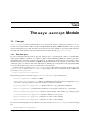
on coupled, non-linear, time-dependent partial differential equations. It consists of five major components:
• esys.escript core library
• finite element solvers esys.finley, esys.dudley, esys.ripley, and esys.speckley (which
use fast vendor-supplied solvers or the included PASO linear solver library)
• the meshing interface esys.pycad
• a model library
• an inversion module.
All esys.escript modules should work under both python 2 and python 3, see Appendix E. The current
version supports parallelization through MPI for distributed memory, OpenMP for shared memory on CPUs, as
well as CUDA for some GPU-based solvers.
This release comes with some significant changes and new features. Please see Appendix B for a detailed list.
If you use this software in your research, then we would appreciate (but do not require) a citation. Some
relevant references can be found in Appendix D.
4
Researchers and Developers
Escript is the product of years of work by many people. The active researchers for the current release series (4.x)
are listed here in alphabetical order. While development is collaborative, each person is listed with some of their
major contributions — this list is not exhaustive. Personel for previous release series are listed in an appendix of
the user guide.
Cihan Altinay esys.weipa visualisation package, SCons build system rework, esys.ripley and CUDA
solvers.
Joel Fenwick Lazy evaluation, maintenance of escript module, release wrangler.
Lutz Gross Patriarch, technical lead, solvers, large chunks of the original code.
Jaco du Plessis Symbolic toolbox, GMSH reader MPI implementation, DC resistivity.
Simon Shaw esys.speckley module, release help, large cluster improvements.
5
6
Contents
1
2
3
Tutorial: Solving PDEs
1.1 Installation . . . . . . . . . . . . . .
1.2 The First Steps . . . . . . . . . . . .
1.2.1 Plotting Using matplotlib
1.2.2 Visualization using export files
1.3 The Diffusion Problem . . . . . . . .
1.3.1 Outline . . . . . . . . . . . .
1.3.2 Temperature Diffusion . . . .
1.3.3 Helmholtz Problem . . . . . .
1.3.4 The Transition Problem . . .
1.4 Wave Propagation . . . . . . . . . . .
1.5 Elastic Deformation . . . . . . . . . .
1.6 Stokes Flow . . . . . . . . . . . . . .
1.7 Slip on a Fault . . . . . . . . . . . . .
1.8 Point Sources . . . . . . . . . . . . .
.
.
.
.
.
.
.
.
.
.
.
.
.
.
.
.
.
.
.
.
.
.
.
.
.
.
.
.
.
.
.
.
.
.
.
.
.
.
.
.
.
.
.
.
.
.
.
.
.
.
.
.
.
.
.
.
.
.
.
.
.
.
.
.
.
.
.
.
.
.
.
.
.
.
.
.
.
.
.
.
.
.
.
.
.
.
.
.
.
.
.
.
.
.
.
.
.
.
.
.
.
.
.
.
.
.
.
.
.
.
.
.
.
.
.
.
.
.
.
.
.
.
.
.
.
.
.
.
.
.
.
.
.
.
.
.
.
.
.
.
.
.
.
.
.
.
.
.
.
.
.
.
.
.
.
.
.
.
.
.
.
.
.
.
.
.
.
.
.
.
.
.
.
.
.
.
.
.
.
.
.
.
.
.
.
.
.
.
.
.
.
.
.
.
.
.
.
.
.
.
.
.
.
.
.
.
.
.
.
.
.
.
.
.
.
.
.
.
.
.
.
.
.
.
.
.
.
.
.
.
.
.
.
.
.
.
.
.
.
.
.
.
.
.
.
.
.
.
.
.
.
.
.
.
.
.
.
.
.
.
.
.
.
.
.
.
.
.
.
.
.
.
.
.
.
.
.
.
.
.
.
.
.
.
.
.
.
.
.
.
.
.
.
.
.
.
.
.
.
.
.
.
.
.
.
.
.
.
.
.
.
.
.
.
.
.
.
.
.
.
.
.
.
.
.
.
.
.
.
.
.
.
.
.
.
.
.
.
.
.
.
.
.
.
.
.
.
.
.
.
.
.
.
.
.
.
.
.
.
.
.
.
.
.
.
.
.
.
.
.
.
.
.
.
.
.
.
.
.
.
.
.
.
.
.
.
.
.
.
.
.
.
.
.
.
.
.
.
.
.
.
.
.
.
.
.
.
.
.
.
.
.
.
.
.
.
.
.
.
.
.
.
.
.
.
.
.
.
.
.
.
.
.
.
.
.
.
.
.
.
.
.
.
.
.
.
.
.
11
11
11
15
17
18
18
18
19
21
23
30
32
35
38
Execution of an escript Script
2.1 Overview . . . . . . . . . .
2.2 Options . . . . . . . . . . .
2.2.1 Notes . . . . . . . .
2.3 Input and Output . . . . . .
2.4 Hints for MPI Programming
2.5 Lazy Evaluation . . . . . . .
.
.
.
.
.
.
.
.
.
.
.
.
.
.
.
.
.
.
.
.
.
.
.
.
.
.
.
.
.
.
.
.
.
.
.
.
.
.
.
.
.
.
.
.
.
.
.
.
.
.
.
.
.
.
.
.
.
.
.
.
.
.
.
.
.
.
.
.
.
.
.
.
.
.
.
.
.
.
.
.
.
.
.
.
.
.
.
.
.
.
.
.
.
.
.
.
.
.
.
.
.
.
.
.
.
.
.
.
.
.
.
.
.
.
.
.
.
.
.
.
.
.
.
.
.
.
.
.
.
.
.
.
.
.
.
.
.
.
.
.
.
.
.
.
.
.
.
.
.
.
.
.
.
.
.
.
.
.
.
.
.
.
.
.
.
.
.
.
.
.
.
.
.
.
.
.
.
.
.
.
.
.
.
.
.
.
.
.
.
.
.
.
41
41
42
42
43
43
44
The esys.escript Module
3.1 Concepts . . . . . . . . . . . . . . . . . . .
3.1.1 Function spaces . . . . . . . . . . . .
3.1.2 Data Objects . . . . . . . . . . . . .
3.1.3 Tagged, Expanded and Constant Data
3.1.4 Saving and Restoring Simulation Data
3.2 esys.escript Classes . . . . . . . . . .
3.2.1 The Domain class . . . . . . . . . .
3.2.2 The FunctionSpace class . . . .
3.2.3 The Data Class . . . . . . . . . . .
3.2.4 Generation of Data objects . . . . .
3.2.5 Generating random Data objects . .
3.2.6 Data methods . . . . . . . . . . . .
3.2.7 Functions of Data objects . . . . . .
3.2.8 Interpolating Data . . . . . . . . . .
3.2.9 The DataManager Class . . . . . .
3.2.10 Saving Data as CSV . . . . . . . . .
.
.
.
.
.
.
.
.
.
.
.
.
.
.
.
.
.
.
.
.
.
.
.
.
.
.
.
.
.
.
.
.
.
.
.
.
.
.
.
.
.
.
.
.
.
.
.
.
.
.
.
.
.
.
.
.
.
.
.
.
.
.
.
.
.
.
.
.
.
.
.
.
.
.
.
.
.
.
.
.
.
.
.
.
.
.
.
.
.
.
.
.
.
.
.
.
.
.
.
.
.
.
.
.
.
.
.
.
.
.
.
.
.
.
.
.
.
.
.
.
.
.
.
.
.
.
.
.
.
.
.
.
.
.
.
.
.
.
.
.
.
.
.
.
.
.
.
.
.
.
.
.
.
.
.
.
.
.
.
.
.
.
.
.
.
.
.
.
.
.
.
.
.
.
.
.
.
.
.
.
.
.
.
.
.
.
.
.
.
.
.
.
.
.
.
.
.
.
.
.
.
.
.
.
.
.
.
.
.
.
.
.
.
.
.
.
.
.
.
.
.
.
.
.
.
.
.
.
.
.
.
.
.
.
.
.
.
.
.
.
.
.
.
.
.
.
.
.
.
.
.
.
.
.
.
.
.
.
.
.
.
.
.
.
.
.
.
.
.
.
.
.
.
.
.
.
.
.
.
.
.
.
.
.
.
.
.
.
.
.
.
.
.
.
.
.
.
.
.
.
.
.
.
.
.
.
.
.
.
.
.
.
.
.
.
.
.
.
.
.
.
.
.
.
.
.
.
.
.
.
.
.
.
.
.
.
.
.
.
.
.
.
.
.
.
.
.
.
.
.
.
.
.
.
.
.
.
.
.
.
.
.
.
.
.
.
.
.
.
.
.
.
.
.
.
.
.
.
.
.
.
.
.
.
.
.
.
.
.
.
.
.
.
.
.
.
.
.
.
.
.
.
.
.
.
.
.
.
.
.
.
.
.
.
.
.
.
.
.
.
.
.
.
.
.
.
.
.
.
.
.
.
.
.
.
.
.
.
.
.
.
.
.
.
.
.
.
.
45
45
45
47
48
49
50
50
51
53
54
54
56
56
62
64
65
Contents
.
.
.
.
.
.
.
.
.
.
.
.
.
.
.
.
.
.
.
.
.
.
.
.
.
.
.
.
.
.
7
3.3
3.4
4
5
6
7
8
3.2.11 The Operator Class . . . . . . . . . . . . . . . . . . . . . . . . . . . . . . . . . . . .
Physical Units . . . . . . . . . . . . . . . . . . . . . . . . . . . . . . . . . . . . . . . . . . . . .
Utilities . . . . . . . . . . . . . . . . . . . . . . . . . . . . . . . . . . . . . . . . . . . . . . . .
66
66
69
The esys.escript.linearPDEs Module
4.1 Linear Partial Differential Equations . . .
4.1.1 Classes . . . . . . . . . . . . . .
4.1.2 LinearPDE class . . . . . . . .
4.1.3 The Poisson Class . . . . . . .
4.1.4 The Helmholtz Class . . . . .
4.1.5 The Lame Class . . . . . . . . .
4.2 Projection . . . . . . . . . . . . . . . . .
4.3 Solver Options . . . . . . . . . . . . . .
4.4 Some Remarks on Lumping . . . . . . .
4.4.1 Scalar wave equation . . . . . . .
4.4.2 Advection equation . . . . . . . .
4.4.3 Summary . . . . . . . . . . . . .
.
.
.
.
.
.
.
.
.
.
.
.
.
.
.
.
.
.
.
.
.
.
.
.
.
.
.
.
.
.
.
.
.
.
.
.
.
.
.
.
.
.
.
.
.
.
.
.
.
.
.
.
.
.
.
.
.
.
.
.
.
.
.
.
.
.
.
.
.
.
.
.
.
.
.
.
.
.
.
.
.
.
.
.
.
.
.
.
.
.
.
.
.
.
.
.
.
.
.
.
.
.
.
.
.
.
.
.
.
.
.
.
.
.
.
.
.
.
.
.
.
.
.
.
.
.
.
.
.
.
.
.
.
.
.
.
.
.
.
.
.
.
.
.
.
.
.
.
.
.
.
.
.
.
.
.
.
.
.
.
.
.
.
.
.
.
.
.
.
.
.
.
.
.
.
.
.
.
.
.
.
.
.
.
.
.
.
.
.
.
.
.
.
.
.
.
.
.
.
.
.
.
.
.
.
.
.
.
.
.
.
.
.
.
.
.
.
.
.
.
.
.
.
.
.
.
.
.
.
.
.
.
.
.
.
.
.
.
.
.
.
.
.
.
.
.
.
.
.
.
.
.
.
.
.
.
.
.
.
.
.
.
.
.
.
.
.
.
.
.
.
.
.
.
.
.
.
.
.
.
.
.
.
.
.
.
.
.
.
.
.
.
.
.
.
.
.
.
.
.
.
.
.
.
.
.
.
.
.
.
.
.
.
.
.
.
.
.
.
.
.
.
.
.
.
.
.
.
.
.
.
.
.
.
.
.
.
.
.
.
.
.
.
.
.
.
.
.
.
.
.
.
.
.
.
.
.
.
.
.
71
71
73
73
75
75
76
76
77
84
84
85
87
The esys.pycad Module
5.1 Introduction . . . . . . . . . . . . . . . .
5.2 The Unit Square . . . . . . . . . . . . . .
5.3 Holes . . . . . . . . . . . . . . . . . . .
5.4 A 3D example . . . . . . . . . . . . . . .
5.5 Alternative File Formats . . . . . . . . .
5.6 Element Sizes . . . . . . . . . . . . . . .
5.7 esys.pycad Classes . . . . . . . . . .
5.7.1 Primitives . . . . . . . . . . . . .
5.7.2 Transformations . . . . . . . . .
5.7.3 Properties . . . . . . . . . . . . .
5.8 Interface to the mesh generation software
.
.
.
.
.
.
.
.
.
.
.
.
.
.
.
.
.
.
.
.
.
.
.
.
.
.
.
.
.
.
.
.
.
.
.
.
.
.
.
.
.
.
.
.
.
.
.
.
.
.
.
.
.
.
.
.
.
.
.
.
.
.
.
.
.
.
.
.
.
.
.
.
.
.
.
.
.
.
.
.
.
.
.
.
.
.
.
.
.
.
.
.
.
.
.
.
.
.
.
.
.
.
.
.
.
.
.
.
.
.
.
.
.
.
.
.
.
.
.
.
.
.
.
.
.
.
.
.
.
.
.
.
.
.
.
.
.
.
.
.
.
.
.
.
.
.
.
.
.
.
.
.
.
.
.
.
.
.
.
.
.
.
.
.
.
.
.
.
.
.
.
.
.
.
.
.
.
.
.
.
.
.
.
.
.
.
.
.
.
.
.
.
.
.
.
.
.
.
.
.
.
.
.
.
.
.
.
.
.
.
.
.
.
.
.
.
.
.
.
.
.
.
.
.
.
.
.
.
.
.
.
.
.
.
.
.
.
.
.
.
.
.
.
.
.
.
.
.
.
.
.
.
.
.
.
.
.
.
.
.
.
.
.
.
.
.
.
.
.
.
.
.
.
.
.
.
.
.
.
.
.
.
.
.
.
.
.
.
.
.
.
.
.
.
.
.
.
.
.
.
.
.
.
.
.
.
.
.
.
.
.
.
.
.
.
.
.
.
.
.
.
.
.
.
.
.
.
.
.
.
89
89
89
91
92
93
94
94
94
97
98
99
Models
6.1 The Stokes Problem . . . . . . . . .
6.1.1 Solution Method . . . . . .
6.1.2 Functions . . . . . . . . . .
6.1.3 Example: Lid-driven Cavity
6.2 Darcy Flux . . . . . . . . . . . . .
6.2.1 Solution Method . . . . . .
6.2.2 Functions . . . . . . . . . .
6.2.3 Example: Gravity Flow . . .
6.3 Isotropic Kelvin Material . . . . . .
6.3.1 Solution Method . . . . . .
6.3.2 Functions . . . . . . . . . .
6.4 Fault System . . . . . . . . . . . .
6.4.1 Functions . . . . . . . . . .
6.4.2 Example . . . . . . . . . .
.
.
.
.
.
.
.
.
.
.
.
.
.
.
.
.
.
.
.
.
.
.
.
.
.
.
.
.
.
.
.
.
.
.
.
.
.
.
.
.
.
.
.
.
.
.
.
.
.
.
.
.
.
.
.
.
.
.
.
.
.
.
.
.
.
.
.
.
.
.
.
.
.
.
.
.
.
.
.
.
.
.
.
.
.
.
.
.
.
.
.
.
.
.
.
.
.
.
.
.
.
.
.
.
.
.
.
.
.
.
.
.
.
.
.
.
.
.
.
.
.
.
.
.
.
.
.
.
.
.
.
.
.
.
.
.
.
.
.
.
.
.
.
.
.
.
.
.
.
.
.
.
.
.
.
.
.
.
.
.
.
.
.
.
.
.
.
.
.
.
.
.
.
.
.
.
.
.
.
.
.
.
.
.
.
.
.
.
.
.
.
.
.
.
.
.
.
.
.
.
.
.
.
.
.
.
.
.
.
.
.
.
.
.
.
.
.
.
.
.
.
.
.
.
.
.
.
.
.
.
.
.
.
.
.
.
.
.
.
.
.
.
.
.
.
.
.
.
.
.
.
.
.
.
.
.
.
.
.
.
.
.
.
.
.
.
.
.
.
.
.
.
.
.
.
.
.
.
.
.
.
.
.
.
.
.
.
.
.
.
.
.
.
.
.
.
.
.
.
.
.
.
.
.
.
.
.
.
.
.
.
.
.
.
.
.
.
.
.
.
.
.
.
.
.
.
.
.
.
.
.
.
.
.
.
.
.
.
.
.
.
.
.
.
.
.
.
.
.
.
.
.
.
.
.
.
.
.
.
.
.
.
.
.
.
.
.
.
.
.
.
.
.
.
.
.
.
.
.
.
.
.
.
.
.
.
.
.
.
.
.
.
.
.
.
.
.
.
.
.
.
.
.
.
.
.
.
.
.
.
.
.
.
.
.
.
.
.
.
.
.
.
.
.
.
.
.
.
.
.
.
.
.
.
.
.
.
.
.
.
.
.
.
.
.
.
.
.
.
.
.
.
.
.
.
.
.
.
.
.
.
.
103
103
103
107
108
108
109
109
110
111
112
113
114
116
118
The esys.finley Module
7.1 Formulation . . . . . . . . . . . . . .
7.2 Meshes . . . . . . . . . . . . . . . .
7.3 Macro Elements . . . . . . . . . . . .
7.4 Linear Solvers in SolverOptions .
7.5 Functions . . . . . . . . . . . . . . .
7.6 esys.dudley . . . . . . . . . . . .
.
.
.
.
.
.
.
.
.
.
.
.
.
.
.
.
.
.
.
.
.
.
.
.
.
.
.
.
.
.
.
.
.
.
.
.
.
.
.
.
.
.
.
.
.
.
.
.
.
.
.
.
.
.
.
.
.
.
.
.
.
.
.
.
.
.
.
.
.
.
.
.
.
.
.
.
.
.
.
.
.
.
.
.
.
.
.
.
.
.
.
.
.
.
.
.
.
.
.
.
.
.
.
.
.
.
.
.
.
.
.
.
.
.
.
.
.
.
.
.
.
.
.
.
.
.
.
.
.
.
.
.
.
.
.
.
.
.
.
.
.
.
.
.
.
.
.
.
.
.
.
.
.
.
.
.
.
.
.
.
.
.
.
.
.
.
.
.
.
.
.
.
.
.
.
.
.
.
.
.
.
.
.
.
.
.
.
.
.
.
.
.
119
119
119
126
126
126
128
Contents
8
The esys.ripley Module
8.1 Formulation . . . . . . . . . . . . . .
8.2 Meshes . . . . . . . . . . . . . . . .
8.3 Functions . . . . . . . . . . . . . . .
8.4 Linear Solvers in SolverOptions .
.
.
.
.
.
.
.
.
.
.
.
.
.
.
.
.
.
.
.
.
.
.
.
.
.
.
.
.
.
.
.
.
.
.
.
.
.
.
.
.
.
.
.
.
.
.
.
.
.
.
.
.
.
.
.
.
.
.
.
.
.
.
.
.
.
.
.
.
.
.
.
.
.
.
.
.
.
.
.
.
.
.
.
.
.
.
.
.
.
.
.
.
.
.
.
.
.
.
.
.
.
.
.
.
.
.
.
.
.
.
.
.
.
.
.
.
.
.
.
.
.
.
.
.
.
.
.
.
129
129
130
130
131
The esys.speckley Module
9.1 Formulation . . . . . . . . . . . . . .
9.2 Meshes . . . . . . . . . . . . . . . .
9.3 Linear Solvers in SolverOptions .
9.4 Cross-domain Interpolation . . . . . .
9.5 Functions . . . . . . . . . . . . . . .
.
.
.
.
.
.
.
.
.
.
.
.
.
.
.
.
.
.
.
.
.
.
.
.
.
.
.
.
.
.
.
.
.
.
.
.
.
.
.
.
.
.
.
.
.
.
.
.
.
.
.
.
.
.
.
.
.
.
.
.
.
.
.
.
.
.
.
.
.
.
.
.
.
.
.
.
.
.
.
.
.
.
.
.
.
.
.
.
.
.
.
.
.
.
.
.
.
.
.
.
.
.
.
.
.
.
.
.
.
.
.
.
.
.
.
.
.
.
.
.
.
.
.
.
.
.
.
.
.
.
.
.
.
.
.
.
.
.
.
.
.
.
.
.
.
.
.
.
.
.
.
.
.
.
.
.
.
.
.
.
133
133
133
133
133
134
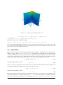
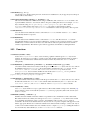
10 The esys.weipa Module and Data Visualization
10.1 The EscriptDataset class . . . . . . . . . . . .
10.2 Functions . . . . . . . . . . . . . . . . . . . . . . .
10.3 Visualizing escript Data . . . . . . . . . . . . . . . .
10.3.1 Using the VisIt GUI . . . . . . . . . . . . . .
10.3.2 Using the VisIt CLI (command line interface)
.
.
.
.
.
.
.
.
.
.
.
.
.
.
.
.
.
.
.
.
.
.
.
.
.
.
.
.
.
.
.
.
.
.
.
.
.
.
.
.
.
.
.
.
.
.
.
.
.
.
.
.
.
.
.
.
.
.
.
.
.
.
.
.
.
.
.
.
.
.
.
.
.
.
.
.
.
.
.
.
.
.
.
.
.
.
.
.
.
.
.
.
.
.
.
.
.
.
.
.
.
.
.
.
.
.
.
.
.
.
.
.
.
.
.
.
.
.
.
.
135
135
136
137
137
138
11 The escript symbolic toolbox
11.1 Introduction . . . . . . . . .
11.2 NonlinearPDE . . . . . . . .
11.3 2D Plane Strain Problem . .
11.4 Classes . . . . . . . . . . .
11.4.1 Symbol class . . . .
11.4.2 Evaluator class . . .
11.4.3 NonlinearPDE class
11.4.4 Symconsts class . .
.
.
.
.
.
.
.
.
.
.
.
.
.
.
.
.
.
.
.
.
.
.
.
.
.
.
.
.
.
.
.
.
.
.
.
.
.
.
.
.
.
.
.
.
.
.
.
.
.
.
.
.
.
.
.
.
.
.
.
.
.
.
.
.
.
.
.
.
.
.
.
.
.
.
.
.
.
.
.
.
.
.
.
.
.
.
.
.
.
.
.
.
.
.
.
.
.
.
.
.
.
.
.
.
.
.
.
.
.
.
.
.
.
.
.
.
.
.
.
.
.
.
.
.
.
.
.
.
.
.
.
.
.
.
.
.
.
.
.
.
.
.
.
.
.
.
.
.
.
.
.
.
.
.
.
.
.
.
.
.
.
.
.
.
.
.
.
.
.
.
.
.
.
.
.
.
.
.
.
.
.
.
.
.
.
.
.
.
.
.
.
.
139
139
139
140
142
142
143
144
144
9
.
.
.
.
.
.
.
.
.
.
.
.
.
.
.
.
.
.
.
.
.
.
.
.
.
.
.
.
.
.
.
.
.
.
.
.
.
.
.
.
.
.
.
.
.
.
.
.
.
.
.
.
.
.
.
.
.
.
.
.
.
.
.
.
.
.
.
.
.
.
.
.
.
.
.
.
.
.
.
.
.
.
.
.
.
.
.
.
.
.
.
.
.
.
.
.
.
.
.
.
.
.
.
.
A Einstein Notation
145
B Changes from previous releases
147
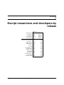
C Escript researchers and developers by release
153
D Escript references
155
E Python3 Support
157
E.1 Impact on scripts . . . . . . . . . . . . . . . . . . . . . . . . . . . . . . . . . . . . . . . . . . . 157
Index
159
Bibliography
163
Contents
9
10
Contents
CHAPTER
ONE
Tutorial: Solving PDEs
1.1
Installation
To download escript and friends, please visit https://launchpad.net/escript-finley. The web site
offers binary distributions for some platforms, source code, documentation including information about the installation process, as well as a way to ask questions.
1.2
The First Steps
In this chapter we give an introduction how to use esys.escript to solve a partial differential equation (PDE).
We assume you are at least a little familiar with python. The knowledge presented in the python tutorial at https:
//docs.python.org/2/tutorial/ is more than sufficient.
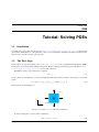
The PDE we wish to solve is the Poisson equation
− ∆u = f
(1.1)
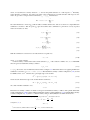
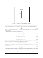
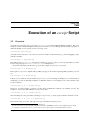
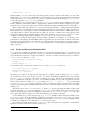
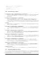
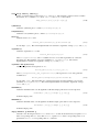
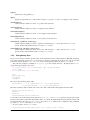
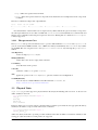
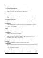
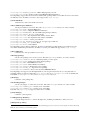
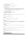
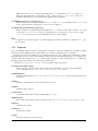
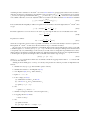
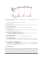
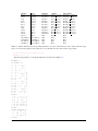
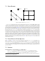
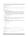
for the solution u. The function f is the given right hand side. The domain of interest, denoted by Ω, is the unit
square
Ω = [0, 1]2 = {(x0 ; x1 )|0 ≤ x0 ≤ 1 and 0 ≤ x1 ≤ 1}
(1.2)
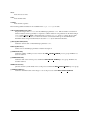
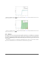
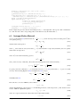
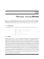
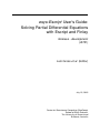
The domain is shown in Figure 1.1.
n
(1, 1)
x1
(0, 0)
x0
F IGURE 1.1: Domain Ω = [0, 1]2 with outer normal field n.
∆ denotes the Laplace operator, which is defined by
∆u = (u,0 ),0 + (u,1 ),1
Chapter 1. Tutorial: Solving PDEs
(1.3)
11
where, for any function u and any direction i, u,i denotes the partial derivative of u with respect to i.1 Basically,
in the subindex of a function, any index to the right of the comma denotes a spatial derivative with respect to the
index. To get a more compact form we will write u,ij = (u,i ),j which leads to
∆u = u,00 + u,11 =
2
X
u,ii
(1.4)
i=0
P
We often find that use of nested
symbols
P makes formulas cumbersome, and we use the more compact Einstein
summation convention. This drops the
sign and assumes that a summation is performed over any repeated
index. For instance we write
xi yi =
2
X
xi yi
(1.5)
xi u,i
(1.6)
i=0
xi u,i =
2
X
i=0
u,ii =
2
X
u,ii
(1.7)
xij ui,j
(1.8)
i=0
xij ui,j =
2 X
2
X
j=0 i=0
(1.9)
With the summation convention we can write the Poisson equation as
− u,ii = 1
(1.10)
where f = 1 in this example.
On the boundary of the domain Ω the normal derivative ni u,i of the solution u shall be zero, i.e. u shall fulfill
the homogeneous Neumann boundary condition
ni u,i = 0 .
(1.11)
n = (ni ) denotes the outer normal field of the domain, see Figure 1.1. Remember that we are applying the Einstein
summation convention , i.e. ni u,i = n0 u,0 + n1 u,1 .2 The Neumann boundary condition of Equation (1.11) should
be fulfilled on the set ΓN which is the top and right edge of the domain:
ΓN = {(x0 ; x1 ) ∈ Ω|x0 = 1 or x1 = 1}
(1.12)
On the bottom and the left edge of the domain which is defined as
ΓD = {(x0 ; x1 ) ∈ Ω|x0 = 0 or x1 = 0}
(1.13)
the solution shall be identical to zero:
u=0.
(1.14)
This kind of boundary condition is called a homogeneous Dirichlet boundary condition. The partial differential
equation in Equation (1.10) together with the Neumann boundary condition Equation (1.11) and Dirichlet boundary
condition in Equation (1.14) form a so-called boundary value problem (BVP) for the unknown function u.
1 You
may be more familiar with the Laplace operator being written as ∇2 , and written in the form
∇2 u = ∇t · ∇u =
∂2u
∂2u
+
2
∂x0
∂x21
and Equation (1.1) as
−∇2 u = f
2 Some
12
readers may familiar with the notation
∂u
∂n
= ni u,i for the normal derivative.
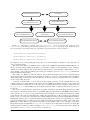
1.2. The First Steps
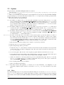
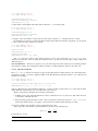
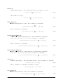
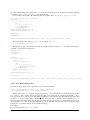
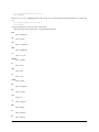
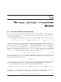
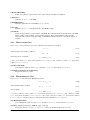
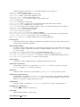
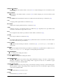
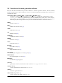
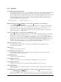
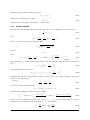
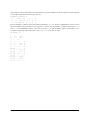
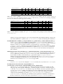
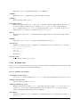
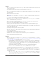
Node
Element
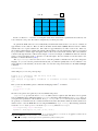
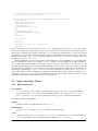
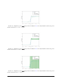
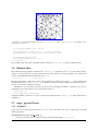
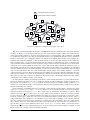
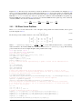
F IGURE 1.2: Mesh of 4 × 4 elements on a rectangular domain. Here each element is a quadrilateral and described by four
nodes, namely the corner points. The solution is interpolated by a bi-linear polynomial.
In general the BVP cannot be solved analytically and numerical methods have to be used to construct an
approximation of the solution u. Here we will use the finite element method (FEM). The basic idea is to fill the
domain with a set of points called nodes. The solution is approximated by its values on the nodes. Moreover,
the domain is subdivided into smaller sub-domains called elements. On each element the solution is represented
by a polynomial of a certain degree through its values at the nodes located in the element. The nodes and their
connection through elements is called a mesh. Figure 1.2 shows an example of a FEM mesh with four elements
in the x0 and four elements in the x1 direction over the unit square. For more details we refer the reader to the
literature, for instance Reference [40, 5].
The esys.escript solver we want to use to solve this problem is embedded into the python interpreter
language. So you can solve the problem interactively but you will learn quickly that it is more efficient to use
scripts which you can edit with your favorite editor. To enter the escript environment, use the run-escript
command3 :
run-escript
which will pass you on to the python prompt
Python 2.7.6 (default, Mar 22 2014, 15:40:47)
[GCC 4.8.2] on linux2
Type "help", "copyright", "credits" or "license" for more information.
>>>
Here you can use all available python commands and language features4 , for instance
>>> x=2+3
>>> print("2+3=",x)
2+3= 5
We refer to the python user’s guide if you are not familiar with python.
esys.escript provides the class Poisson to define a Poisson equation. (We will discuss a more general
form of a PDE that can be defined through the LinearPDE class later.) The instantiation of a Poisson class object requires the specification of the domain Ω. In esys.escript the Domain class objects are used to describe
the geometry of a domain but it also contains information about the discretization methods and the actual solver
which is used to solve the PDE. Here we are using the FEM library esys.finley. The following statements
create the Domain object mydomain from the esys.finley function Rectangle:
from esys.finley import Rectangle
mydomain = Rectangle(l0=1.,l1=1.,n0=40, n1=20)
3 run-escript is not available under Windows. If you run under Windows you can just use the python command and the
OMP NUM THREADS environment variable to control the number of threads.
4 Throughout our examples, we use the python 3 form of print. That is, print(1) instead of print 1.
Chapter 1. Tutorial: Solving PDEs
13
In this case the domain is a rectangle with the lower left corner at point (0, 0) and the upper right corner at
(l0, l1) = (1, 1). The arguments n0 and n1 define the number of elements in x0 and x1 -direction respectively.
For more details on Rectangle and other Domain generators see Chapter 7, Chapter 8, and Chapter 9.
The following statements define the Poisson class object mypde with domain mydomain and the right
hand side f of the PDE to constant 1:
from esys.escript.linearPDEs import Poisson
mypde = Poisson(mydomain)
mypde.setValue(f=1)
We have not specified any boundary condition but the Poisson class implicitly assumes homogeneous Neuman
boundary conditions defined by Equation (1.11). With this boundary condition the BVP we have defined has no
unique solution. In fact, with any solution u and any constant C the function u + C becomes a solution as well. We
have to add a Dirichlet boundary condition. This is done by defining a characteristic function which has positive
values at locations x = (x0 , x1 ) where Dirichlet boundary condition is set and 0 elsewhere. In our case of ΓD
defined by Equation (1.13), we need to construct a function gammaD which is positive for the cases x0 = 0 or
x1 = 0. To get an object x which contains the coordinates of the nodes in the domain use
x=mydomain.getX()
The method getX of the Domain mydomain gives access to locations in the domain defined by mydomain.
The object x is actually a Data object which will be discussed in Chapter 3 in more detail. What we need to know
here is that x has rank (number of dimensions) and a shape (list of dimensions) which can be viewed by calling
the getRank and getShape methods:
print("rank ",x.getRank(),", shape ",x.getShape())
This will print something like
rank 1, shape (2,)
The Data object also maintains type information which is represented by the FunctionSpace of the object.
For instance
print(x.getFunctionSpace())
will print
Finley_Nodes [ContinuousFunction(domain)] on FinleyMesh
which tells us that the coordinates are stored on the nodes of (rather than on points in the interior of) a Finley mesh.
To get the x0 coordinates of the locations we use the statement
x0=x[0]
Object x0 is again a Data object now with rank 0 and shape (). It inherits the FunctionSpace from x:
print(x0.getRank(), x0.getShape(), x0.getFunctionSpace())
will print
0 () Finley_Nodes [ContinuousFunction(domain)] on FinleyMesh
We can now construct a function gammaD which is only non-zero on the bottom and left edges of the domain with
from esys.escript import whereZero
gammaD=whereZero(x[0])+whereZero(x[1])
whereZero(x[0]) creates a function which equals 1 where x[0] is (almost) equal to zero and 0 elsewhere. Similarly, whereZero(x[1]) creates a function which equals 1 where x[1] is equal to zero and 0
elsewhere. The sum of the results of whereZero(x[0]) and whereZero(x[1]) gives a function on the
domain mydomain which is strictly positive where x0 or x1 is equal to zero. Note that gammaD has the same
rank , shape and FunctionSpace like x0 used to define it. So from
print(gammaD.getRank(), gammaD.getShape(), gammaD.getFunctionSpace())
one gets
0 () Finley_Nodes [ContinuousFunction(domain)] on FinleyMesh
14
1.2. The First Steps
An additional parameter q of the setValue method of the Poisson class defines the characteristic function of
the locations of the domain where the homogeneous Dirichlet boundary condition is set. The complete definition
of our example is now:
from esys.escript.linearPDEs import Poisson
x = mydomain.getX()
gammaD = whereZero(x[0])+whereZero(x[1])
mypde = Poisson(domain=mydomain)
mypde.setValue(f=1,q=gammaD)
The first statement imports the Poisson class definition from the esys.escript.linearPDEs module. To
get the solution of the Poisson equation defined by mypde we just have to call its getSolution method.
Now we can write the script to solve our Poisson problem
from esys.escript import *
from esys.escript.linearPDEs import Poisson
from esys.finley import Rectangle
# generate domain:
mydomain = Rectangle(l0=1.,l1=1.,n0=40, n1=20)
# define characteristic function of GammaˆD
x = mydomain.getX()
gammaD = whereZero(x[0])+whereZero(x[1])
# define PDE and get its solution u
mypde = Poisson(domain=mydomain)
mypde.setValue(f=1, q=gammaD)
u = mypde.getSolution()
The question is what we do with the calculated solution u. Besides postprocessing, e.g. calculating the gradient
or the average value, which will be discussed later, plotting the solution is one of the things you might want to
do. esys.escript offers two ways to do this, both based on external modules or packages. The first option is
using the matplotlib module which allows plotting 2D results relatively quickly from within the python script,
see [16]. However, there are limitations when using this tool, especially for large problems and when solving
three-dimensional problems. Therefore, esys.escript provides functionality to export data as files which can
subsequently be read by third-party software packages such as Mayavi2 [18] or VisIt [36].
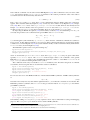
1.2.1
Plotting Using matplotlib
The matplotlib module provides a simple and easy-to-use way to visualize PDE solutions (or other Data objects). To hand over data from esys.escript to matplotlib the values need to be mapped onto a rectangular
grid. We will make use of the numpy module for this.
First we need to create a rectangular grid which is accomplished by the following statements:
import numpy
x_grid = numpy.linspace(0., 1., 50)
y_grid = numpy.linspace(0., 1., 50)
x_grid is an array defining the x coordinates of the grid while y_grid defines the y coordinates of the grid. In
this case we use 50 points over the interval [0, 1] in both directions.
Now the values created by esys.escript need to be interpolated to this grid. We will use the matplotlib
mlab.griddata function to do this. Spatial coordinates are easily extracted as a list by
x=mydomain.getX()[0].toListOfTuples()
y=mydomain.getX()[1].toListOfTuples()
In principle we can apply the same toListOfTuples method to extract the values from the PDE solution u.
However, we have to make sure that the Data object we extract the values from uses the same FunctionSpace
as we have used when extracting x and y. We apply the interpolation to u before extraction to achieve this:
z=interpolate(u, mydomain.getX().getFunctionSpace())
The values in z are the values at the points with the coordinates given by x and y. These values are interpolated to
the grid defined by x_grid and y_grid by using
import matplotlib
z_grid = matplotlib.mlab.griddata(x, y, z, xi=x_grid, yi=y_grid)
Chapter 1. Tutorial: Solving PDEs
15
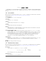
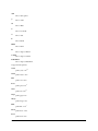
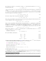
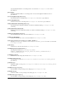
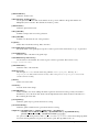
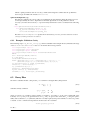
1.0
0.8
0.6
0.4
0.2
0.0
0.0
0.2
0.4
0.6
0.8
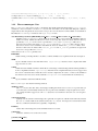
1.0
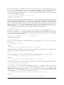
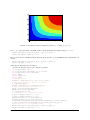
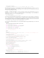
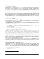
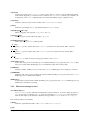
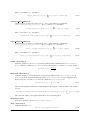
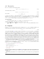
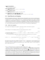
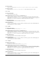
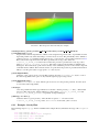
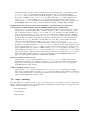
F IGURE 1.3: Visualization of the Poisson Equation Solution for f = 1 using matplotlib
Now z_grid gives the values of the PDE solution u at the grid which can be plotted using contourf:
matplotlib.pyplot.contourf(x_grid, y_grid, z_grid, 5)
matplotlib.pyplot.savefig("u.png")
Here we use 5 contours. The last statement writes the plot to the file u.png in the PNG format. Alternatively, one
can use
matplotlib.pyplot.contourf(x_grid, y_grid, z_grid, 5)
matplotlib.pyplot.show()
which gives an interactive browser window.
Now we can write the script to solve our Poisson problem
from esys.escript import *
from esys.escript.linearPDEs import Poisson
from esys.finley import Rectangle
import numpy
import matplotlib
import pylab
# generate domain:
mydomain = Rectangle(l0=1.,l1=1.,n0=40, n1=20)
# define characteristic function of GammaˆD
x = mydomain.getX()
gammaD = whereZero(x[0])+whereZero(x[1])
# define PDE and get its solution u
mypde = Poisson(domain=mydomain)
mypde.setValue(f=1,q=gammaD)
u = mypde.getSolution()
# interpolate u to a matplotlib grid:
x_grid = numpy.linspace(0.,1.,50)
y_grid = numpy.linspace(0.,1.,50)
x=mydomain.getX()[0].toListOfTuples()
y=mydomain.getX()[1].toListOfTuples()
z=interpolate(u,mydomain.getX().getFunctionSpace()).toListOfTuples()
z_grid = matplotlib.mlab.griddata(x,y,z,xi=x_grid,yi=y_grid )
# interpolate u to a rectangular grid:
matplotlib.pyplot.contourf(x_grid, y_grid, z_grid, 5)
matplotlib.pyplot.savefig("u.png")
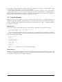
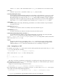
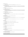
16
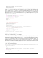
1.2. The First Steps
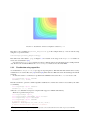
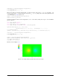
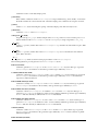
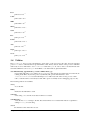
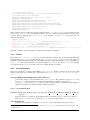
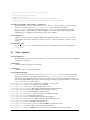
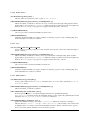
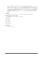
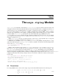
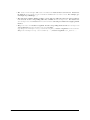
F IGURE 1.4: Visualization of the Poisson Equation Solution for f = 1
The entire code is available as poisson_matplotlib.py in the example directory. You can run the script
using the escript environment
run-escript poisson_matplotlib.py
This will create a file called u.png, see Figure 1.3. For details on the usage of the matplotlib module we
refer to the documentation [16].
As pointed out, matplotlib is restricted to the two-dimensional case and should be used for small problems
only. It can not be used under MPI as the toListOfTuples method is not safe under MPI5 .
1.2.2
Visualization using export files
As an alternative to matplotlib, escript supports exporting data to VTK and SILO files which can be read by
visualization tools such as Mayavi2 [18] and VisIt [36]. This method is MPI safe and works with large 2D and 3D
problems.
To write the solution u of the Poisson problem in the VTK file format to the file u.vtu one needs to add:
from esys.weipa import saveVTK
saveVTK("u.vtu", sol=u)
This file can then be opened in a VTK compatible visualization tool where the solution is accessible by the name
sol. Similarly,
from esys.weipa import saveSilo
saveSilo("u.silo", sol=u)
will write u to a SILO file if escript was compiled with support for LLNL’s SILO library.
The Poisson problem script is now
from esys.escript import *
from esys.escript.linearPDEs import Poisson
from esys.finley import Rectangle
from esys.weipa import saveVTK
# generate domain:
mydomain = Rectangle(l0=1.,l1=1.,n0=40, n1=20)
# define characteristic function of GammaˆD
5 The
phrase ’safe under MPI’ means that a program will produce correct results when run on more than one processor under MPI.
Chapter 1. Tutorial: Solving PDEs
17
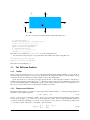
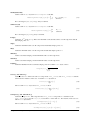
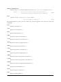
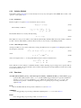
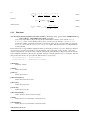
Tref
n
x1
x0
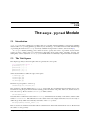
F IGURE 1.5: Temperature Diffusion Problem with Circular Heat Source
x = mydomain.getX()
gammaD = whereZero(x[0])+whereZero(x[1])
# define PDE and get its solution u
mypde = Poisson(domain=mydomain)
mypde.setValue(f=1,q=gammaD)
u = mypde.getSolution()
# write u to an external file
saveVTK("u.vtu",sol=u)
The entire code is available as poisson_vtk.py in the example directory.
You can run the script using the escript environment and visualize the solution using Mayavi2:
run-escript poisson_vtk.py
mayavi2 -d u.vtu -m Surface
The result is shown in Figure 1.4.
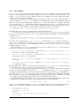
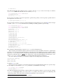
1.3
1.3.1
The Diffusion Problem
Outline
In this section we will discuss how to solve a time-dependent temperature diffusion PDE for a given block of
material. Within the block there is a heat source which drives the temperature diffusion. On the surface, energy
can radiate into the surrounding environment. Figure 1.5 shows the configuration.
In the next Section 1.3.2 we will present the relevant model. A time integration scheme is introduced to
calculate the temperature at given time nodes t(n) . We will see that at each time step a Helmholtz equation must
be solved. The implementation of a Helmholtz equation solver will be discussed in Section 1.3.3. In Section 1.3.4
this solver is used to build a solver for the temperature diffusion problem.
1.3.2
Temperature Diffusion
The unknown temperature T is a function of its location in the domain and time t > 0. The governing equation in
the interior of the domain is given by
ρcp T,t − (κT,i ),i = qH
(1.15)
where ρcp and κ are given material constants. In case of a composite material the parameters depend on their
location in the domain. qH is a heat source (or sink) within the domain. We are using the Einstein summation
convention as introduced in Chapter 1.2. In our case we assume qH to be equal to a constant heat production rate
q c on a circle or sphere with center xc and radius r, and 0 elsewhere:
c
q
if kx − xc k ≤ r
qH (x, t) =
(1.16)
0
else
18
1.3. The Diffusion Problem
for all x in the domain and time t > 0.
On the surface of the domain we specify a radiation condition which prescribes the normal component of the
flux κT,i to be proportional to the difference of the current temperature to the surrounding temperature Tref :
κT,i ni = η(Tref − T )
(1.17)
η is a given material coefficient depending on the material of the block and the surrounding medium. ni is the i-th
component of the outer normal field at the surface of the domain.
To solve the time-dependent Equation (1.15) the initial temperature at time t = 0 has to be given. Here we
assume that the initial temperature is the surrounding temperature:
T (x, 0) = Tref
(1.18)
for all x in the domain. Note that the initial conditions satisfy the boundary condition defined by Equation (1.17).
The temperature is calculated at discrete time nodes t(n) where t(0) = 0 and t(n) = t(n−1) + h, where h > 0
is the step size which is assumed to be constant. In the following, the upper index (n) refers to a value at time t(n) .
The simplest and most robust scheme to approximate the time derivative of the temperature is the backward Euler
scheme. The backward Euler scheme is based on the Taylor expansion of T at time t(n) :
(n)
(n)
T (n) ≈ T (n−1) + T,t (t(n) − t(n−1) ) = T (n−1) + h · T,t
(1.19)
This is inserted into Equation (1.15). By separating the terms at t(n) and t(n−1) one gets for n = 1, 2, 3 . . .
ρcp (n−1)
ρcp (n)
(n)
T
− (κT,i ),i = qH +
T
h
h
(1.20)
where T (0) = Tref is taken form the initial condition given by Equation (1.18). Together with the natural boundary
condition
(n)
κT,i ni = η(Tref − T (n) )
(1.21)
taken from Equation (1.17) this forms a boundary value problem that has to be solved for each time step. As a
first step to implement a solver for the temperature diffusion problem we will implement a solver for the boundary
value problem that has to be solved at each time step.
1.3.3
Helmholtz Problem
The partial differential equation to be solved for T (n) has the form
(n)
ωT (n) − (κT,i ),i = f
and we set
ρcp
ρcp (n−1)
and f = qH +
T
.
h
h
the radiation condition defined by Equation (1.21) takes the form
ω=
With g = ηTref
(n)
κT,i ni = g − ηT (n) on Γ
(1.22)
(1.23)
(1.24)
The partial differential Equation (1.22) together with boundary conditions of Equation (1.24) is called the Helmholtz
equation.
We want to use the LinearPDE class provided by esys.escript to define and solve a general linear,
steady, second order PDE such as the Helmholtz equation. For a single PDE the LinearPDE class supports the
following form:
− (Ajl u,l ),j + Du = Y
(1.25)
where we show only the coefficients relevant for the problem discussed here. For the general form of a single
PDE see Equation (4.1). The coefficients A and Y have to be specified through Data objects in the general
FunctionSpace on the PDE or objects that can be converted into such Data objects. A is a rank-2 Data
object and D and Y are scalar. The following natural boundary conditions are considered on Γ:
nj Ajl u,l + du = y .
Chapter 1. Tutorial: Solving PDEs
(1.26)
19
Notice that the coefficient A is the same as in the PDE Equation (1.25). The coefficients d and y are each a scalar
Data object in the boundary FunctionSpace. Constraints for the solution prescribe the value of the solution
at certain locations in the domain. They have the form
u = r where q > 0
(1.27)
Both r and q are a scalar Data object where q is the characteristic function defining where the constraint is
applied. The constraints defined by Equation (1.27) override any other condition set by Equation (1.25) or Equation (1.26). The Poisson class of the esys.escript.linearPDEs module, which we have already used in
Chapter 1.2, is in fact a subclass of the more general LinearPDE class. The esys.escript.linearPDEs
module provides a Helmholtz class but we will make direct use of the general LinearPDE class.
By inspecting the Helmholtz equation (1.22) and boundary condition (1.24), and substituting u for T (n) , we
can easily assign values to the coefficients in the general PDE of the LinearPDE class:
Aij = κδij
d=η
D=ω
y=g
Y =f
(1.28)
δij is the Kronecker symbol defined by δij = 1 for i = j and 0 otherwise. Undefined coefficients are assumed to
be not present.6 In this diffusion example we do not need to define a characteristic function q because the boundary
conditions we consider in Equation (1.24) are just the natural boundary conditions which are already defined in the
LinearPDE class (shown in Equation (1.26)).
The Helmholtz equation can be set up the following way7 :
mypde=LinearPDE(mydomain)
mypde.setValue(A=kappa*kronecker(mydomain),D=omega,Y=f,d=eta,y=g)
u=mypde.getSolution()
where we assume that mydomain is a Domain object and kappa, omega, eta, and g are given scalar values
typically float or Data objects. The setValue method assigns values to the coefficients of the general
PDE. The getSolution method solves the PDE and returns the solution u of the PDE. kronecker is an
esys.escript function returning the Kronecker symbol.
The coefficients can be set by several calls to setValue in arbitrary order. If a value is assigned to a coefficient
several times, the last assigned value is used when the solution is calculated:
mypde = LinearPDE(mydomain)
mypde.setValue(A=kappa*kronecker(mydomain), d=eta)
mypde.setValue(D=omega, Y=f, y=g)
mypde.setValue(d=2*eta) # overwrites d=eta
u=mypde.getSolution()
In some cases the solver of the PDE can make use of the fact that the PDE is symmetric. A PDE is called symmetric
if
Ajl = Alj .
(1.29)
Note that D and d may have any value and the right hand sides Y , y as well as the constraints are not relevant. The
Helmholtz problem is symmetric. The LinearPDE class provides the method checkSymmetry to check if the
given PDE is symmetric.
mypde = LinearPDE(mydomain)
mypde.setValue(A=kappa*kronecker(mydomain), d=eta)
print(mypde.checkSymmetry()) # returns True
mypde.setValue(B=kronecker(mydomain)[0])
print(mypde.checkSymmetry()) # returns False
mypde.setValue(C=kronecker(mydomain)[0])
print(mypde.checkSymmetry()) # returns True
Unfortunately, calling checkSymmetry is very expensive and is only recommended for testing and debugging
purposes. The setSymmetryOn method is used to declare a PDE symmetric:
6 There
is a difference in esys.escript for a coefficient to be not present and set to zero. Since in the former case the coefficient is not
processed, it is more efficient to leave it undefined instead of assigning zero to it.
7 Note that this is not a complete code. The full source code can be found in “helmholtz.py”.
20
1.3. The Diffusion Problem
mypde = LinearPDE(mydomain)
mypde.setValue(A=kappa*kronecker(mydomain))
mypde.setSymmetryOn()
Now we want to see how we actually solve the Helmholtz equation on a rectangular domain of length l0 = 5 and
height l1 = 1. We choose a simple test solution such that we can verify the returned solution against the exact
answer. Actually, we take T = x0 (here qH = 0) and then calculate the right hand side terms f and g such that
the test solution becomes the solution of the problem. If we assume κ as being constant, an easy calculation shows
that we have to choose f = ω · x0 . On the boundary we get κni u,i = κn0 . Thus we have to set g = κn0 + ηx0 .
The following script helmholtz.py which is available in the example directory implements this test problem
using the esys.finley PDE solver:
from esys.escript import *
from esys.escript.linearPDEs import LinearPDE
from esys.finley import Rectangle
from esys.weipa import saveVTK
# set some parameters
kappa=1.
omega=0.1
eta=10.
# generate domain
mydomain = Rectangle(l0=5., l1=1., n0=50, n1=10)
# open PDE and set coefficients
mypde=LinearPDE(mydomain)
mypde.setSymmetryOn()
n=mydomain.getNormal()
x=mydomain.getX()
mypde.setValue(A=kappa*kronecker(mydomain), D=omega,Y=omega*x[0], \
d=eta, y=kappa*n[0]+eta*x[0])
# calculate error of the PDE solution
u=mypde.getSolution()
print("error is ",Lsup(u-x[0]))
saveVTK("x0.vtu", sol=u)
To visualize the solution ‘x0.vtu’ you can use the command
mayavi2 -d x0.vtu -m Surface
and it is easy to see that the solution T = x0 is calculated.
The script is similar to the script poisson.py discussed in Chapter 1.2. mydomain.getNormal()
returns the outer normal field on the surface of the domain. The function Lsup is imported by the from
esys.escript import * statement and returns the maximum absolute value of its argument. The error
shown by the print statement should be in the order of 10−7 . As piecewise bi-linear interpolation is used by
esys.finley to approximate the solution, and our solution is a linear function of the spatial coordinates, one
might expect that the error would be zero or in the order of machine precision (typically ≈ 10−15 ). However most
PDE packages use an iterative solver which is terminated when a given tolerance has been reached. The default
tolerance is 10−8 . This value can be altered by using the setTolerance method of the LinearPDE class.
1.3.4
The Transition Problem
Now we are ready to solve the original time-dependent problem. The main part of the script is the loop over time
t which takes the following form:
t=0
T=Tref
mypde=LinearPDE(mydomain)
mypde.setValue(A=kappa*kronecker(mydomain), D=rhocp/h, d=eta, y=eta*Tref)
while t<t_end:
mypde.setValue(Y=q+rhocp/h*T)
T=mypde.getSolution()
t+=h
Chapter 1. Tutorial: Solving PDEs
21
kappa, rhocp, eta and Tref are input parameters of the model. q is the heat source in the domain and h
is the time step size. The variable T holds the current temperature. It is used to calculate the right hand side
coefficient f in the Helmholtz Equation (1.22). The statement T=mypde.getSolution() overwrites T with
the temperature of the new time step t + h. To get this iterative process going we need to specify the initial
temperature distribution, which is equal to Tref . The LinearPDE object mypde and the coefficients that do not
change over time are set up before the loop is entered. In each time step only the coefficient Y is reset as it depends
on the temperature of the previous time step. This allows the PDE solver to reuse information from previous time
steps as much as possible.
The heat source qH which is defined in Equation (1.16) is qc in an area defined as a circle of radius r and
center xc, and zero outside this circle. q0 is a fixed constant. The following script defines qH as desired:
from esys.escript import length,whereNegative
xc=[0.02, 0.002]
r=0.001
x=mydomain.getX()
qH=q0*whereNegative(length(x-xc)-r)
x is a Data object of the esys.escript module defining locations in the Domain mydomain. The length()
function imported from the esys.escript module returns the Euclidean norm:
kyk =
√
yi yi = esys.escript.length(y)
(1.30)
So length(x-xc) calculates the distances of the location x to the center of the circle xc where the heat source
is acting. Note that the coordinates of xc are defined as a list of floating point numbers. It is automatically
converted into a Data class object before being subtracted from x. The function whereNegative applied to
length(x-xc)-r returns a Data object which is equal to one where the object is negative (inside the circle)
and zero elsewhere. After multiplication with qc we get a function with the desired property of having value qc
inside the circle and zero elsewhere.
Now we can put the components together to create the script diffusion.py which is available in the example directory :
from esys.escript import *
from esys.escript.linearPDEs import LinearPDE
from esys.finley import Rectangle
from esys.weipa import saveVTK
#... set some parameters ...
xc=[0.02, 0.002]
r=0.001
qc=50.e6
Tref=0.
rhocp=2.6e6
eta=75.
kappa=240.
tend=5.
# ... time, time step size and counter ...
t=0
h=0.1
i=0
#... generate domain ...
mydomain = Rectangle(l0=0.05, l1=0.01, n0=250, n1=50)
#... open PDE ...
mypde=LinearPDE(mydomain)
mypde.setSymmetryOn()
mypde.setValue(A=kappa*kronecker(mydomain), D=rhocp/h, d=eta, y=eta*Tref)
# ... set heat source: ....
x=mydomain.getX()
qH=qc*whereNegative(length(x-xc)-r)
# ... set initial temperature ....
T=Tref
# ... start iteration:
while t<tend:
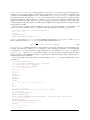
22
1.3. The Diffusion Problem
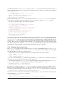
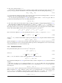
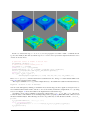
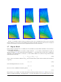
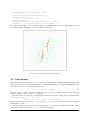
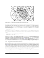
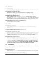
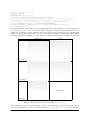
F IGURE 1.6: Results of the Temperature Diffusion Problem for Time Steps 1, 16, 32 and 48 (top to bottom)
i+=1
t+=h
print("time step:",t)
mypde.setValue(Y=qH+rhocp/h*T)
T=mypde.getSolution()
saveVTK("T.%d.vtu"%i, temp=T)
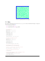
The script will create the files T.1.vtu, T.2.vtu, . . ., T.50.vtu in the directory where the script has been
started. The files contain the temperature distributions at time steps 1, 2, i, . . . , 50 in the VTK file format.
Figure 1.6 shows the result for some selected time steps. An easy way to visualize the results is the command
mayavi2 -d T.1.vtu -m Surface
Use the Configure Data window in Mayavi2 to move forward and backward in time.
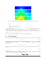
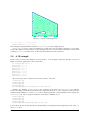
1.4
Wave Propagation
In this next example we want to calculate the displacement field ui for any time t > 0 by solving the wave equation:
ρui,tt − σij,j = 0
(1.31)
in a three dimensional block of length L in x0 and x1 direction and height H in x2 direction. ρ is the known
density which may be a function of its location. σij is the stress field which in case of an isotropic, linear elastic
material is given by
σij = λuk,k δij + µ(ui,j + uj,i )
(1.32)
where λ and µ are the Lam´e coefficients and δij denotes the Kronecker symbol. On the boundary the normal stress
is given by
σij nj = 0
(1.33)
for all time t > 0.
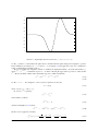
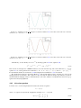
Here we are modelling a point source at the point xC in the x0 -direction which is a negative pulse of amplitude
U0 followed by the same positive pulse. In mathematical terms we use
u0 (xC , t) = U0
Chapter 1. Tutorial: Solving PDEs
√ (t − t0 ) 1 − (t−t0 )2
α2
2
e2
α
(1.34)
23
1
0.8
0.6
0.4
0.2
0
-0.2
-0.4
-0.6
-0.8
-1
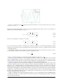
0
1
2
3
4
5
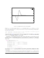
F IGURE 1.7: Input Displacement at Source Point (α = 0.7, t0 = 3, U0 = 1).
for all t ≥ 0 where α is the width of the pulse and t0 is the time when the pulse changes from negative to positive.
In the simulations we will choose α = 0.3 and t0 = 2 (see Figure 1.7) and apply the source as a constraint in a
sphere of small radius around the point xC .
We use an explicit time integration scheme to calculate the displacement field u at certain time marks t(n) ,
where t(n) = t(n−1) + h with time step size h > 0. In the following the upper index (n) refers to values at time
t(n) . We use the Verlet scheme with constant time step size h which is defined by
u(n) = 2u(n−1) − u(n−2) + h2 a(n)
(1.35)
(1.36)
for all n = 2, 3, . . .. It is designed to solve a system of equations of the form
u,tt = G(u)
(1.37)
where one sets a(n) = G(u(n−1) ).
In our case a(n) is given by
(n)
ρai
(n−1)
= σij,j
(1.38)
and boundary conditions
(n−1)
σij
nj = 0
(1.39)
derived from Equation (1.33) where
(n−1)
σij
(n−1)
=
λuk,k
(n−1)
δij + µ(ui,j
(n−1)
+ uj,i
).
(1.40)
We also need to apply the constraint
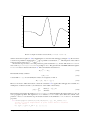
(n)
a0 (xC , t) = U0
24
p
(2.) (t − t0 )3
t − t0 21 − (t−t20 )2
α
(4
−6
)e
2
3
α
α
α
(1.41)
1.4. Wave Propagation
10
8
6
4
2
0
-2
-4
-6
-8
-10
0
1
2
3
4
5
F IGURE 1.8: Input Acceleration at Source Point (α = 0.7, t0 = 3, U0 = 1).
which is derived from equation 1.34 by calculating the second order time derivative (see Figure 1.8). Now we have
converted our problem for displacement, u(n) , into a problem for acceleration, a(n) , which depends on the solution
at the previous two time steps u(n−1) and u(n−2) .
In each time step we have to solve this problem to get the acceleration a(n) , and we will use the LinearPDE
class of the esys.escript.linearPDEs package to do so. The general form of the PDE defined through the
LinearPDE class is discussed in Section 4.1. The form which is relevant here is
(n)
Dij aj
= −Xij,j .
(1.42)
The natural boundary condition
nj Xij = 0
(n)
is used. With u = a
(1.43)
we can identify the values to be assigned to D and X:
Dij = ρδij
(n−1)
Xij = −σij
(1.44)
Moreover we need to define the location r where the constraint 1.41 is applied. We will apply the constraint on a
small sphere of radius R around xC (we will use 3% of the width of the domain):
1
where kx − xc k ≤ R
qi (x) =
(1.45)
0
otherwise.
The following script defines the function wavePropagation which implements the Verlet scheme to solve our
wave propagation problem. The argument domain which is a Domain class object defines the domain of the
problem. h and tend are the time step size and the end time of the simulation. lam, mu and rho are material
properties.
def wavePropagation(domain,h,tend,lam,mu,rho, x_c, src_radius, U0):
# lists to collect displacement at point source which is returned
# to the caller
ts, u_pc0, u_pc1, u_pc2 = [], [], [], []
Chapter 1. Tutorial: Solving PDEs
25
x=domain.getX()
# ... open new PDE ...
mypde=LinearPDE(domain)
mypde.getSolverOptions().setSolverMethod(SolverOptions.HRZ_LUMPING)
kronecker=identity(mypde.getDim())
dunit=numpy.array([1., 0., 0.]) # defines direction of point source
mypde.setValue(D=kronecker*rho, q=whereNegative(length(x-xc)-src_radius)*dunit)
# ... set initial values ....
n=0
# for first two time steps
u=Vector(0., Solution(domain))
u_last=Vector(0., Solution(domain))
t=0
# define the location of the point source
L=Locator(domain, xc)
# find potential at point source
u_pc=L.getValue(u)
print("u at point charge=",u_pc)
ts.append(t)
u_pc0.append(u_pc[0])
u_pc1.append(u_pc[1])
u_pc2.append(u_pc[2])
while t<tend:
t+=h
# ... get current stress ....
g=grad(u)
stress=lam*trace(g)*kronecker+mu*(g+transpose(g))
# ... get new acceleration ....
amplitude=U0*(4*(t-t0)**3/alpha**3-6*(t-t0)/alpha)*sqrt(2.)/alpha**2 \
*exp(1./2.-(t-t0)**2/alpha**2)
mypde.setValue(X=-stress, r=dunit*amplitude)
a=mypde.getSolution()
# ... get new displacement ...
u_new=2*u-u_last+h**2*a
# ... shift displacements ....
u_last=u
u=u_new
n+=1
print(n,"-th time step, t=",t)
u_pc=L.getValue(u)
print("u at point charge=",u_pc)
# save displacements at point source to file for t > 0
ts.append(t)
u_pc0.append(u_pc[0])
u_pc1.append(u_pc[1])
u_pc2.append(u_pc[2])
# ... save current acceleration in units of gravity and displacements
if n==1 or n%10==0:
saveVTK("./data/usoln.%i.vtu"%(n/10), \
acceleration = length(a)/9.81, \
displacement = length(u), \
tensor = stress, Ux = u[0])
return ts, u_pc0, u_pc1, u_pc2
Notice that all coefficients of the PDE which are independent of time t are set outside the while loop. This is for
efficiency reasons since it allows the LinearPDE class to reuse information as much as possible when iterating
over time.
The statement
26
1.4. Wave Propagation
mypde.getSolverOptions().setSolverMethod(SolverOptions.HRZ_LUMPING)
enables the use of an aggressive approximation of the PDE operator as a diagonal matrix formed from the coefficient D. The approximation allows, at the cost of additional error, very fast solution of the PDE, see also
Section 4.4.
There are a few new esys.escript functions in this example: grad(u) returns the gradient ui,j of u
(in fact grad(g)[i,j] == ui,j ). There are restrictions on the argument of the grad function, for instance
the statement grad(grad(u)) will raise an exception. trace(g) returns the sum of the main diagonal elements g[k,k] of g and transpose(g) returns the matrix transpose of g (i.e. transpose(g)[i,j] ==
g[j,i]).
We initialize the values of u and u_last to be zero. It is important to initialize both with the solution
FunctionSpace as they have to be seen as solutions of PDEs from previous time steps. In fact, the grad does
not accept arguments with a certain FunctionSpace, for more details see Section 3.2.3.
The Locator class is designed to extract values at a given location (in this case xC ) from functions such as
the displacement vector u. Typically Locator is used in the following way:
L=Locator(domain, xc)
u=...
u_pc=L.getValue(u)
The return value u_pc is the value of u at the location xc8 . The values are collected in the lists u_pc0, u_pc1
and u_pc2 together with the corresponding time marker in ts. These values are handed back to the caller. Later
we will show ways to access these data.
One of the big advantages of the Verlet scheme is the fact that the problem to be solved in each time step is very
simple and does not involve any spatial derivatives (which is what allows us to use lumping in this simulation).
The problem becomes so simple because we use the stress from the last time step rather than the stress which is
actually present at the current time step. Schemes using this approach are called explicit time integration schemes.
The backward Euler scheme we have used in Chapter 1.3 is an example of an implicit scheme. In this case one uses
the actual status of each variable at a particular time rather than values from previous time steps. This will lead to
a problem which is more expensive to solve, in particular for non-linear cases. Although explicit time integration
schemes are cheap to finalize a single time step, they need significantly smaller time steps than implicit schemes
and can suffer from stability problems. Therefore they require a very careful selection of the time step size h.
An easy, heuristic way of choosing an appropriate time step size is the Courant-Friedrichs-Lewy condition
(CFL condition) which says that within a time step information should not travel further than a cell
q used in the
discretization scheme. In the case of the wave equation the velocity of a (p-) wave is given as
should choose h from
r
1
ρ
∆x
h=
5 λ + 2µ
λ+2µ
ρ
so one
(1.46)
where ∆x is the cell diameter. The factor 51 is a safety factor considering the heuristics of the formula.
The following script uses the wavePropagation function to solve the wave equation for a point source
located at the bottom face of a block. The width of the block in each direction on the bottom face is 10km (x0 and
x1 directions, i.e. l0 and l1). The variable ne gives the number of elements in x0 and x1 directions. The depth
of the block is aligned with the x2 -direction. The depth (l2) of the block in the x2 -direction is chosen so that
there are 10 elements, and the magnitude of the depth is chosen such that the elements become cubic. We chose
10 for the number of elements in the x2 -direction so that the computation is faster. Brick(n0 , n1 , n2 , l0 , l1 , l2 )
is an esys.finley function which creates a rectangular mesh with n0 × n1 × n2 elements over the brick
[0, l0 ] × [0, l1 ] × [0, l2 ].
from esys.finley import Brick
ne = 32
# number of cells in x_0 and x_1 directions
width = 10000.
# length in x_0 and x_1 directions
lam = 3.462e9
mu = 3.462e9
rho = 1154.
tend = 60
U0 = 1. # amplitude of point source
8 In
fact, it is the finite element node which is closest to the given position. The usage of Locator is MPI safe.
Chapter 1. Tutorial: Solving PDEs
27
F IGURE 1.9: Selected time steps (n = 11, 22, 32, 36) of a wave propagation over a 10km × 10km × 3.125km block from
a point source initially at (5km, 5km, 0) with time step size h = 0.02083. Color represents the displacement. Here the view is
oriented onto the bottom face.
# spherical source at middle of bottom face
xc=[width/2.,width/2.,0.]
# define small radius around point xc
src_radius = 0.03*width
print("src_radius =",src_radius)
mydomain=Brick(ne, ne, 10, l0=width, l1=width, l2=10.*width/32.)
h=(1./5.)*inf(sqrt(rho/(lam+2*mu))*inf(domain.getSize())
print("time step size =",h)
ts, u_pc0, u_pc1, u_pc2 = \
wavePropagation(mydomain, h, tend, lam, mu, rho, xc, src_radius, U0)
The domain.getSize() function returns the local element size ∆x. Using inf ensures that the CFL condition 1.46 holds everywhere in the domain.
The script is available as wave.py in the example directory . To visualize the results from the data directory:
mayavi2 -d usoln.1.vtu -m Surface
You can rotate this figure by clicking on it with the mouse and moving it around. Again use Configure Data to
move backward and forward in time, and also to choose the results (acceleration, displacement or ux ) by using
Select Scalar. Figure 1.9 shows the results for the displacement at various time steps.
It remains to show some possibilities to inspect the collected data u_pc0, u_pc1 and u_pc2. One way is
to write the data to a file and then use an external package such as gnuplot[39], LibreOffice Calc or Excel to read
the data for further analysis. The following code shows one possible way to write the data to the file ./data/U_
pc.csv:
u_pc_data=FileWriter('./data/U_pc.csv')
for i in range(len(ts)):
u_pc_data.write("%f %f %f %f\n"%(ts[i],u_pc0[i],u_pc1[i],u_pc2[i]))
u_pc_data.close()
28
1.4. Wave Propagation
1.5
U_x
U_y
U_z
1
0.5
0
-0.5
-1
-1.5
0
2
4
6
8
10
F IGURE 1.10: Amplitude at Point source from the Simulation
The file U_pc.csv stores 4 columns of data: t, ux , uy , uz respectively, where ux , uy , uz are the x0 , x1 , x2 components of the displacement vector u at the point source. These can be plotted easily using any plotting package.
In gnuplot[39] the command:
plot 'U_pc.csv' u 1:2 title 'U_x' w l lw 2, 'U_pc.csv' u 1:3 title 'U_y' w l
lw 2, 'U_pc.csv' u 1:4 title 'U_z' w l lw 2
will reproduce Figure 1.10 (As expected this is identical to the input signal shown in Figure 1.7). It is pointed
out that we are not using the standard python open to write to the file U_pc.csv as it is not safe when running
esys.escript under MPI, see Chapter 2 for more details.
Alternatively, one can implement plotting the results at run time rather than in a post-processing step. This
avoids the generation of an intermediate data file. In escript the preferred way of creating 2D plots of time dependent data is matplotlib. The following script creates the plot and writes it into the file u_pc.png in the PNG
image format:
import matplotlib.pyplot as plt
if getMPIRankWorld() == 0:
plt.title("Displacement at Point Source")
plt.plot(ts, u_pc0, '-', label="x_0", linewidth=1)
plt.plot(ts, u_pc1, '-', label="x_1", linewidth=1)
plt.plot(ts, u_pc2, '-', label="x_2", linewidth=1)
plt.xlabel('time')
plt.ylabel('displacement')
plt.legend()
plt.savefig('u_pc.png', format='png')
You can add plt.show() to create an interactive browser window. Notice that by checking the condition
getMPIRankWorld()==0 the plot is generated on one processor only (in this case the rank 0 processor) when
run under MPI.
Both options for processing the point source data are included in the example file wave.py. There are other
options available to process these data in particular through the SciPy[35] package, e.g. Fourier transformations. It
Chapter 1. Tutorial: Solving PDEs
29
is beyond the scope of this user’s guide to document the usage of SciPy[35] for time series analysis but it is highly
recommended to look in relevant readily available documentation.
1.5
Elastic Deformation
In this section we want to examine the deformation of a linear elastic body caused by expansion through a heat
distribution. We want a displacement field ui which solves the momentum equation:
−σij,j = 0
(1.47)
2
σij = λuk,k δij + µ(ui,j + uj,i ) − (λ + µ) α (T − Tref )δij .
3
(1.48)
where the stress σ is given by
In this formula λ and µ are the Lam´e coefficients, α is the temperature expansion coefficient, T is the temperature
distribution and Tref a reference temperature. Note that Equation (1.47) is similar to Equation (1.31) introduced
in Section 1.4 but the inertia term ρui,tt has been dropped as we assume a static scenario here. Moreover, in
comparison to the Equation (1.32) definition of stress σ in Equation (1.48) an extra term is introduced to bring in
stress due to volume changes through temperature dependent expansion.
Our domain is the unit cube
Ω = {(xi )|0 ≤ xi ≤ 1}
(1.49)
On the boundary the normal stress component is set to zero
σij nj = 0
(1.50)
and on the face with xi = 0 we set the i-th component of the displacement to 0:
ui (x) = 0
where
xi = 0
(1.51)
k
(1.52)
For the temperature distribution we use
T (x) = T0 e−βkx−x
c
with a given positive constant β and location xc in the domain.
When we insert Equation (1.48) we get a second order system of linear PDEs for the displacements u which is
called the Lam´e equation. We want to solve this using the LinearPDE class. For a system of PDEs and a solution
with several components the LinearPDE class takes PDEs of the form
− (Aijkl uk,l ),j = −Xij,j .
(1.53)
A is a rank-4 Data object and X is a rank-2 Data object. We show here the coefficients relevant for the problem
we are trying to solve. The full form is given in Equation (4.4). The natural boundary conditions take the form
nj Aijkl uk,l = nj Xij
(1.54)
ui = ri where qi > 0
(1.55)
while constraints take the form
r and q are each a rank-1 Data object. We can easily identify the coefficients in Equation (1.53):
Aijkl = λδij δkl + µ(δik δjl + δil δjk )
2
Xij = (λ + µ) α (T − Tref )δij
3
(1.56)
(1.57)
(1.58)
The characteristic function q defining the locations and components where constraints are set is given by:
1 xi = 0
qi (x) =
0 otherwise.
30
(1.59)
1.5. Elastic Deformation
Under the assumption that λ, µ, β and Tref are constant we may use Yi = (λ + 23 µ) α Ti . However, this choice
would lead to a different natural boundary condition which does not set the normal stress component as defined in
Equation (1.48) to zero.
Analogous to the concept of symmetry for a single PDE, we call the PDE defined by Equation (1.53) symmetric
if
Aijkl = Aklij
(1.60)
(1.61)
This Lam´e equation is in fact symmetric, given the difference in D and d as compared to the scalar case. The
LinearPDE class is notified of this fact by calling its setSymmetryOn method.
After we have solved the Lam´e equation we want to analyse the actual stress distribution. Typically the vonMises stress defined by
r
1
2 + σ2 + σ2 )
(1.62)
((σ00 − σ11 )2 + (σ11 − σ22 )2 + (σ22 − σ00 )2 ) + 3(σ01
σmises =
20
12
2
is used to detect material damage. Here we want to calculate the von-Mises stress and write it to a file for visualization.
The following script, which is available in heatedblock.py in the example directory, solves the Lam´e
equation and writes the displacements and the von-Mises stress into a file deform.vtu in the VTK file format:
from esys.escript import *
from esys.escript.linearPDEs import LinearPDE
from esys.finley import Brick
from esys.weipa import saveVTK
#... set some parameters ...
lam=1.
mu=0.1
alpha=1.e-6
xc=[0.3, 0.3, 1.]
beta=8.
T_ref=0.
T_0=1.
#... generate domain ...
mydomain = Brick(l0=1., l1=1., l2=1., n0=10, n1=10, n2=10)
x=mydomain.getX()
#... set temperature ...
T=T_0*exp(-beta*length(x-xc))
#... open symmetric PDE ...
mypde=LinearPDE(mydomain)
mypde.setSymmetryOn()
#... set coefficients ...
C=Tensor4(0., Function(mydomain))
for i in range(mydomain.getDim()):
for j in range(mydomain.getDim()):
C[i,i,j,j]+=lam
C[i,j,i,j]+=mu
C[i,j,j,i]+=mu
msk=whereZero(x[0])*[1.,0.,0.] \
+whereZero(x[1])*[0.,1.,0.] \
+whereZero(x[2])*[0.,0.,1.]
sigma0=(lam+2./3.*mu)*alpha*(T-T_ref)*kronecker(mydomain)
mypde.setValue(A=C, X=sigma0, q=msk)
#... solve pde ...
u=mypde.getSolution()
#... calculate von-Mises stress
g=grad(u)
sigma=mu*(g+transpose(g))+lam*trace(g)*kronecker(mydomain)-sigma0
sigma_mises=sqrt(((sigma[0,0]-sigma[1,1])**2+(sigma[1,1]-sigma[2,2])**2+ \
(sigma[2,2]-sigma[0,0])**2)/2. \
Chapter 1. Tutorial: Solving PDEs
31
F IGURE 1.11: von-Mises Stress and Displacement Vectors
+3*(sigma[0,1]**2 + sigma[1,2]**2 + sigma[2,0]**2))
#... output ...
saveVTK("deform.vtu", disp=u, stress=sigma_mises)
Finally, the results can be visualized by calling
mayavi2 -d deform.vtu -f CellToPointData -m Vectors -m Surface
Note that the filter CellToPointData is applied to create a smoother representation of the von-Mises stress. Figure 1.11 shows the results where the colour of the vertical planes represent the von-Mises stress and a horizontal
plane of arrows shows the displacements vectors.
1.6
Stokes Flow
In this section we will look at Computational Fluid Dynamics (CFD) to simulate the flow of fluid under the
influence of gravity. The StokesProblemCartesian class will be used to calculate the velocity and pressure
of the fluid. The fluid dynamics is governed by the Stokes equation. In geophysical problems the velocity of fluids
is low; that is, the inertial forces are small compared with the viscous forces, therefore the inertial terms in the
Navier-Stokes equations can be ignored. For a body force f , the governing equations are given by:
∇ · (η(∇~v + ∇T ~v )) − ∇p = −f,
(1.63)
∇ · ~v = 0.
(1.64)
with the incompressibility condition
where p, η and f are the pressure, viscosity and body forces, respectively. Alternatively, the Stokes equations can
be represented in Einstein summation tensor notation (compact notation):
− (η(vi,j + vj,i )),j −p,i = fi ,
(1.65)
− vi,i = 0.
(1.66)
with the incompressibility condition
The subscript comma i denotes the derivative of the function with respect to xi . The body force f in Equation (1.65)
is the gravity acting in the x3 direction and is given as f = −gρδi3 . The Stokes equation is a saddle point problem,
and can be solved using a Uzawa scheme. A class called StokesProblemCartesian in esys.escript
32
1.6. Stokes Flow
can be used to solve for velocity and pressure. A more detailed discussion of the class can be found in Chapter
6. In order to keep numerical stability and satisfy the Courant-Friedrichs-Lewy condition (CFL condition), the
time-step size needs to be kept below a certain value. The Courant number is defined as:
C=
vδt
h
(1.67)
where δt, v, and h are the time-step, velocity, and the width of an element in the mesh, respectively. The velocity
v may be chosen as the maximum velocity in the domain. In this problem the time-step size was calculated for a
Courant number of 0.4.
The following python script is the setup for the Stokes flow simulation, and is available in the example directory
as fluid.py. It starts off by importing the classes, such as the StokesProblemCartesian class, for solving
the Stokes equation and the incompressibility condition for velocity and pressure. Physical constants are defined
for the viscosity and density of the fluid, along with the acceleration due to gravity. Solver settings are set for
the maximum iterations and tolerance; the default solver used is PCG (Preconditioned Conjugate Gradients). The
mesh is defined as a rectangle to represent the body of fluid. We are using 20 × 20 elements with piecewise linear
elements for the pressure and for velocity but the elements are subdivided for the velocity. This approach is called
macro elements and needs to be applied to make sure that the discretized problem has a unique solution, see [13]
for details9 . The fact that pressure and velocity are represented in different ways is expressed by
velocity=Vector(0., Solution(mesh))
pressure=Scalar(0., ReducedSolution(mesh))
The gravitational force is calculated based on the fluid density and the acceleration due to gravity. The boundary
conditions are set for a slip condition at the base and the left face of the domain. At the base fluid movement in the
x0 -direction is free, but fixed in the x1 -direction, and similarly at the left face fluid movement in the x1 -direction
is free but fixed in the x0 -direction. An instance of the StokesProblemCartesian class is defined for the
given computational mesh, and the solver tolerance set. Inside the while loop, the boundary conditions, viscosity
and body force are initialized. The Stokes equation is then solved for velocity and pressure. The time-step size is
calculated based on the Courant-Friedrichs-Lewy condition (CFL condition), to ensure stable solutions. The nodes
in the mesh are then displaced based on the current velocity and time-step size, to move the body of fluid. The
output for the simulation of velocity and pressure is then saved to a file for visualization.
from esys.escript import *
import esys.finley
from esys.escript.linearPDEs import LinearPDE
from esys.escript.models import StokesProblemCartesian
from esys.weipa import saveVTK
# physical constants
eta=1.
rho=100.
g=10.
# solver settings
tolerance=1.0e-4
max_iter=200
t_end=50
t=0.0
time=0
verbose=True
# define mesh
H=2.
L=1.
W=1.
mesh = esys.finley.Rectangle(l0=L, l1=H, order=-1, n0=20, n1=20)
coordinates = mesh.getX()
9 Alternatively, one can use second order elements for the velocity and first order elements for pressure on the same element. You can set
order=2 in esys.finley.Rectangle.
Chapter 1. Tutorial: Solving PDEs
33
# gravitational force
Y=Vector(0., Function(mesh))
Y[1] = -rho*g
# element spacing
h = Lsup(mesh.getSize())
# boundary conditions for slip at base
boundary_cond=whereZero(coordinates[1])*[0.0,1.0]+whereZero(coordinates[0])*[1.0,0.0]
# velocity and pressure vectors
velocity=Vector(0., Solution(mesh))
pressure=Scalar(0., ReducedSolution(mesh))
# Stokes Cartesian
solution=StokesProblemCartesian(mesh)
solution.setTolerance(tolerance)
while t <= t_end:
print(" ----- Time step = %s -----"%t)
print("Time = %s seconds"%time)
solution.initialize(fixed_u_mask=boundary_cond, eta=eta, f=Y)
velocity,pressure=solution.solve(velocity,pressure,max_iter=max_iter, \
verbose=verbose)
print("Max velocity =", Lsup(velocity), "m/s")
# CFL condition
dt=0.4*h/(Lsup(velocity))
print("dt =", dt)
# displace the mesh
displacement = velocity * dt
coordinates = mesh.getX()
newx=interpolate(coordinates + displacement, ContinuousFunction(mesh))
mesh.setX(newx)
time += dt
vel_mag = length(velocity)
#save velocity and pressure output
saveVTK("vel.%2.2i.vtu"%t, vel=vel_mag, vec=velocity, pressure=pressure)
t = t+1.
The results from the simulation can be viewed with Mayavi2, by executing the following command:
mayavi2 -d vel.00.vtu -m Surface
Colour-coded scalar maps and velocity flow fields can be viewed by selecting them in the menu. The time-steps
can be swept through to view a movie of the simulation. Figure 1.12 shows the simulation output. Velocity vectors
and a colour map for pressure are shown. As the time progresses the body of fluid falls under the influence of
gravity. The view used here to track the fluid is the Lagrangian view, since the mesh moves with the fluid. One of
the disadvantages of using the Lagrangian view is that the elements in the mesh become severely distorted after a
period of time and introduce solver errors. To get around this limitation the Level Set Method can be used, with
the Eulerian point of view for a fixed mesh.
34
1.7. Slip on a Fault
(a) t=1
(b) t=20
(d) t=40
(e) t=50
(c) t=30
(f) t=60
F IGURE 1.12: Simulation output for Stokes flow. Fluid body starts off as a rectangular shape, then progresses downwards
under the influence of gravity. Colour coded distribution represents the scalar values for pressure. Velocity vectors are displayed
at each node in the mesh to show the flow field. Computational mesh used was 20×20 elements.
1.7
Slip on a Fault
In this example we illustrate how to calculate the stress distribution around a fault in the Earth’s crust caused by a
slip through an earthquake.
To simplify the presentation we assume a simple domain Ω = [0, 1]2 with a vertical fault in its center as
illustrated in Figure 1.13. We assume that the slip distribution si on the fault is known. We want to calculate the
distribution of the displacements ui and stress σij in the domain. Further, we assume an isotropic, linear elastic
material model of the form
σij
= λuk,k δij + µ(ui,j + uj,i )
(1.68)
where λ and µ are the Lam´e coefficients and δij denotes the Kronecker symbol. On the boundary the normal stress
is given by
σij nj = 0
(1.69)
ui ni = 0
(1.70)
and normal displacements are set to zero:
The stress needs to fulfill the momentum equation
−σij,j = 0
(1.71)
This problem is very similar to the elastic deformation problem presented in Section 1.5. However, we need to
address an additional challenge: the displacement ui is in fact discontinuous across the fault, but we are in the
Chapter 1. Tutorial: Solving PDEs
35
(1, 1)
(0.5, 0.75)
Fault
(0.5, 0.25)
(0, 0)
F IGURE 1.13: Domain Ω = [0, 1]2 with a vertical fault of length 0.5.
lucky situation that we know the jump of the displacements across the fault. This is in fact the given slip si . So we
can split the total distribution ui into a component vi which is continuous across the fault and the known slip si
1
ui = vi + s±
2 i
(1.72)
where s± = s when right of the fault and s± = −s when left of the fault. We assume that s± = 0 when sufficiently
away from the fault.
We insert this into the stress definition in Equation (1.68)
σij
=
1 s
c
σij
+ σij
2
(1.73)
with
c
σij
= λvk,k δij + µ(vi,j + vj,i )
(1.74)
±
±
s
σij
= λs±
k,k δij + µ(si,j + sj,i ).
(1.75)
and
s
In fact, σij
defines a stress jump across the fault. An easy way to construct this function is to use a function χ
which is 1 on the right and −1 on the left side from the fault. One can then set
s
σij
= χ · (λsk,k δij + µ(si,j + sj,i ))
(1.76)
assuming that s is extended by zero away from the fault. After inserting Equation (1.73) into (1.71) we get the
differential equation
c
−σij,j
=
1 s
σ
2 ij,j
(1.77)
Together with the definition (1.74) we have a differential equation for the continuous function vi . Notice that the
c
boundary condition (1.70) and (1.69) transfer to vi and σij
as s is zero away from the fault. In Section 1.5 we have
discussed how this problem is solved using the LinearPDE class. We refer to this section for further details.
To define the fault we use the FaultSystem class introduced in Section 6.4. The following statements define
a fault system fs and add the fault 1 to the system:
36
1.7. Slip on a Fault
fs=FaultSystem(dim=2)
fs.addFault(fs.addFault(V0=[0.5,0.25], strikes=90*DEG, ls=0.5, tag=1)
The fault added starts at point (0.5, 0.25) has length 0.5 and points north. The main purpose of the FaultSystem
class is to define a parameterization of the fault using a local coordinate system. One can inquire the class to get
the range used to parameterize a fault.
p0,p1 = fs.getW0Range(tag=1)
Typically p0 is equal to zero while p1 is equal to the length of the fault. The parameterization is given as a
mapping from a set of local coordinates onto a parameter range (in our case the range p0 to p1). For instance, to
map the entire domain mydomain onto the fault one can use
x = mydomain.getX()
p,m = fs.getParametrization(x, tag=1)
Of course there is the problem that not all locations are on the fault. For those locations which are on the fault m is
set to 1, otherwise 0 is used. So on return the values of p define the value of the fault parameterization (typically
the distance from the starting point of the fault along the fault) where m is positive. On all other locations the value
of p is undefined. Now p can be used to define a slip distribution on the fault via
s = m*(p-p0)*(p1-p)/((p1-p0)/2)**2*slip_max*[0.,1.]
Notice the factor m which ensures that s is zero away from the fault. It is important that the slip is zero at the ends
of the faults.
We can now put all components together to get the script:
from
from
from
from
from
from
esys.escript import *
esys.escript.linearPDEs import LinearPDE
esys.escript.models import FaultSystem
esys.finley import Rectangle
esys.weipa import saveVTK
esys.escript.unitsSI import DEG
#... set some parameters ...
lam=1.
mu=1
slip_max=1.
mydomain = Rectangle(l0=1.,l1=1.,n0=16, n1=16) # n1 needs to be a multiple of 4!
# .. create the fault system
fs=FaultSystem(dim=2)
fs.addFault(V0=[0.5,0.25], strikes=90*DEG, ls=0.5, tag=1)
# ... create a slip distribution on the fault
p, m=fs.getParametrization(mydomain.getX(), tag=1)
p0,p1= fs.getW0Range(tag=1)
s=m*(p-p0)*(p1-p)/((p1-p0)/2)**2*slip_max*[0.,1.]
# ... calculate stress according to slip:
D=symmetric(grad(s))
chi, d=fs.getSideAndDistance(D.getFunctionSpace().getX(), tag=1)
sigma_s=(mu*D+lam*trace(D)*kronecker(mydomain))*chi
#... open symmetric PDE ...
mypde=LinearPDE(mydomain)
mypde.setSymmetryOn()
#... set coefficients ...
C=Tensor4(0., Function(mydomain))
for i in range(mydomain.getDim()):
for j in range(mydomain.getDim()):
C[i,i,j,j]+=lam
C[j,i,j,i]+=mu
C[j,i,i,j]+=mu
# ... fix displacement in normal direction
x=mydomain.getX()
msk=whereZero(x[0])*[1.,0.] + whereZero(x[0]-1.)*[1.,0.] \
+whereZero(x[1])*[0.,1.] + whereZero(x[1]-1.)*[0.,1.]
Chapter 1. Tutorial: Solving PDEs
37
mypde.setValue(A=C, X=-0.5*sigma_s, q=msk)
#... solve pde ...
mypde.getSolverOptions().setVerbosityOn()
v=mypde.getSolution()
# .. write the displacement to file:
D=symmetric(grad(v))
sigma=(mu*D+lam*trace(D)*kronecker(mydomain))+0.5*sigma_s
saveVTK("slip.vtu", disp=v+0.5*chi*s, stress=sigma)
The script creates the file slip.vtu which contains the total displacements and stress. These values are stored
as cell-centered data. See Figure 1.14 for a visualization of the result.
F IGURE 1.14: Total Displacement after the slip event
1.8
Point Sources
In the chapter we will show the usage of point sources and sinks. A simple example is a blockm of material with
heat source at a location p and heat sink at a location q. Under the assumption of a constant conductivity the steady
heat diffusion equation for the temperature u is given as
− u,ii = s(pin ) δpin + s(p1 ) δp1
(1.78)
where δpin and δpout refer to the Dirac δ-function and s(pin ) and s(pout ) define the heat production and heat
extraction rates at locations pin and pout , respectively.
First the locations of point sources and sinks need to be added to the domain. This is done at generation time:
mydomain=Rectangle(30,30, l0=3, l1=2,
diracPoints=[(1.,1.), (2.,1.)],
diracTags=['in', 'out'])
In this case the points are located at pin = (1., 1.) and pout = (2., 1.). For easier reference the points are tagged
with the name in and out.
The values at the point source locations are defined using a Data object. One possible way to define the values
at the locations defined through the diracPoint list is using tagging:
38
1.8. Point Sources
s=Scalar(0., DiracDeltaFunctions(mydomain))
s.setTaggedValue('in', +1.)
s.setTaggedValue('out', -1.)
Here we set value 1 at locations tagged with in (in this case this is just point pin = (1., 1.) ) and value −1 at
locations tagged with out (in this case this is just point pout = (2., 1.)). The point source in the right hande side
of the PDE Equation (1.78) is then set as
mypde = LinearSinglePDE(domain=mydomain)
mypde.setValue(y_dirac=s)
Under the assumption that we fix the temperature to zero on the entire boundary the script to solve the PDE is
given as follows:
from
from
from
from
esys.escript import *
esys.weipa import *
esys.finley import Rectangle
esys.escript.linearPDEs import LinearSinglePDE
mydomain=Rectangle(30,30, l0=3, l1=2,
diracPoints=[(1.,1.), (2.,1.)], diracTags=['in', 'out'])
x = mydomain.getX()
gammaD = whereZero(x[0])+whereZero(x[1])+whereZero(x[0]-3.)+whereZero(x[1]-2.)
s=Scalar(0., DiracDeltaFunctions(mydomain))
s.setTaggedValue('in', +1.)
s.setTaggedValue('out', -1.)
mypde = LinearSinglePDE(domain=mydomain)
mypde.setValue(q=gammaD, A=kronecker(2), y_dirac=s)
u = mypde.getSolution()
saveVTK("u.vtu",sol=u)
Result is shown in Figure 1.15.
F IGURE 1.15: Results diffusion problem with nodal source and sink.
Chapter 1. Tutorial: Solving PDEs
39
40
1.8. Point Sources
CHAPTER
TWO
Execution of an escript Script
2.1
Overview
A typical way of starting your escript script myscript.py is with the run-escript command1 . This command was renamed from escript (used in previous releases) to avoid clashing with an unrelated program installed by default on some systems. To run your script, issue2
run-escript myscript.py
as already shown in Section 1.2. In some cases it can be useful to work interactively, e.g. when debugging a script,
with the command
run-escript -i myscript.py
This will execute myscript.py and when it completes (or an error occurs), a python prompt will be provided.
To leave the prompt press Control-d (Control-z on MS Windows).
To run the script using four threads (e.g. if you have a multi-core processor) you can use
run-escript -t 4 myscript.py
This requires escript to be compiled with OpenMP [25] support. To run the script using MPI [21] with 8 processes
use
run-escript -p 8 myscript.py
If the processors which are used are multi-core processors or you are working on a multi-processor shared memory
architecture you can use threading in addition to MPI. For instance to run 8 MPI processes with 4 threads each,
use the command
run-escript -p 8 -t 4 myscript.py
In the case of a supercomputer or a cluster, you may wish to distribute the workload over a number of nodes3 . For
example, to use 8 nodes with 4 MPI processes per node, write
run-escript -n 8 -p 4 myscript.py
Since threading has some performance advantages over processes, you may specify a number of threads as well:
run-escript -n 8 -p 2 -t 4 myscript.py
This runs the script on 8 nodes, with 2 processes per node and 4 threads per process.
1 The
run-escript launcher is not supported under MS Windows.
this discussion, it is assumed that run-escript is included in your PATH environment. See the installation guide for details.
3 For simplicity, we will use the term node to refer to either a node in a supercomputer or an individual machine in a cluster
2 For
Chapter 2. Execution of an escript Script
41
2.2
Options
The general form of the run-escript launcher is as follows:
run-escript [ -n nn ] [ -p np ] [ -t nt ] [ -f hostfile ] [ -x ] [ -V ] [ -e ] [ -h ] [ -v ] [ -o ] [ -c ] [ -i ] [ -b
] [ -m tool ] [ file ] [ ARGS ]
where file is the name of a script and ARGS are the arguments to be passed to the script. The run-escript
program will import your current environment variables. If no file is given, then you will be presented with a
regular python prompt (see -i for restrictions).
The options have the following meaning:
-n nn the number of compute nodes nn to be used. The total number of processes being used is nn · np. This
option overrides the value of the ESCRIPT NUM NODES environment variable. If a hostfile is given
(see below), the number of nodes needs to match the number of hosts given in that file. If nn > 1 but escript
is not compiled for MPI, a warning is printed but execution is continued with nn = 1. If -n is not set the
number of hosts in the host file is used. The default value is 1.
-p np the number of MPI processes (per node). The total number of processes to be used is nn · np. This option
overwrites the value of the ESCRIPT NUM PROCS environment variable. If np > 1 but escript is not
compiled for MPI, a warning is printed but execution is continued with np = 1. The default value is 1.
-t nt the number of threads used per process. The option overwrites the value of the ESCRIPT NUM THREADS
environment variable. If nt > 1 but escript is not compiled for OpenMP , a warning is printed but execution
is continued with nt = 1. The default value is 1.
-f hostfile the name of a file with a list of host names. Some systems require to specify the addresses or names of
the compute nodes where MPI processes should be spawned. These addresses or names of the compute
nodes are listed in the file with the name hostfile. If -n is set, the number of different hosts defined in
hostfile must be equal to the number of requested compute nodes nn. The option overwrites the value
of the ESCRIPT HOSTFILE environment variable. By default no host file is used.
-c prints information about the settings used to compile escript and stops execution.
-V prints the version of escript and stops execution.
-h prints a help message and stops execution.
-i executes the script file and switches to interactive mode after the execution is finished or an exception has
occurred. This option is useful for debugging a script. The option cannot be used if more than one process
(nn · np > 1) is used.
-b do not invoke python. This is used to run non-python programs within an environment set for escript.
-e shows additional environment variables and commands used to set up the escript environment. This option
is useful if users wish to execute scripts without using the run-escript command.
-o enables the redirection of messages printed by processors with MPI rank greater than zero to the files
stdout_r.out and stderr_r.out where r is the rank of the processor. The option overwrites the
value of the ESCRIPT STDFILES environment variable.
-x runs everything within a new xterm instance.
-v prints some diagnostic information.
-m tool runs under valgrind. The argument tool must be one of m (for memcheck), c (for callgrind), or h (for
cachegrind). Valgrind output is written to a file under valgrind_logs as reported when escript terminates.
2.2.1
Notes
The run-escript script is now generated at build time taking into account the prelaunch, launcher,
and postlaunch settings passed to scons. This makes it possible to easily customize the script for different
environments, such as batch systems (PBS, SLURM) and different implementations of MPI (Intel, SGI, OpenMPI,
etc.).
42
2.2. Options
2.3
Input and Output
When MPI is used on more than one process (nn · np > 1) no input from the standard input is accepted. Standard
output on any process other than the master process (rank = 0) will be silently discarded by default. Error output
from any processor will be redirected to the node where run-escript has been invoked. If the -o option or
ESCRIPT STDFILES is set4 , then the standard and error output from any process other than the master process
will be written to files of the names stdout_R.out and stderr_R.out (where R is the rank of the process).
If files are created or read by individual MPI processes with information local to the process (e.g. in the dump
function) and more than one process is used (nn · np > 1), the MPI process rank is appended to the file names.
This is to avoid problems if processes are using a shared file system. Files which collect data that are global for all
MPI processors are created by the process with MPI rank 0 only. Users should keep in mind that if the file system
is not shared among the processes, then a file containing global information which is read by all processors needs
to be copied to the local file system(s) before run-escript is invoked.
2.4
Hints for MPI Programming
In general a script based on the esys.escript module does not require modifications to run under MPI. However, one needs to be careful if other modules are used.
When MPI is used on more than one process (nn · np > 1) the user needs to keep in mind that several copies of
his script are executed at the same time5 while data exchange is performed through the esys.escript module.
This has three main implications:
1. most arguments (Data excluded) should have the same values on all processors, e.g. int, float, str
and numpy parameters.
2. the same operations will be called on all processors.
3. different processors may store different amounts of information.
With a few exceptions6 , values of types int, float, str and numpy returned by esys.escript will
have the same value on all processors. If values produced by other modules are used as arguments, the user has
to make sure that the argument values are identical on all processors. For instance, the usage of a random number
generator to create argument values bears the risk that the value may depend on the processor.
Some operations in esys.escript require communication with all processors executing the job. It is
not always obvious which operations these are. For example, Lsup returns the largest value on all processors.
getValue on Locator may refer to a value stored on another processor. For this reason it is better if scripts
do not have conditional operations (which manipulate data) based on which processor the script is on. Crashing or
hanging scripts can be an indication that this has happened.
It is not always possible to divide data evenly amongst processors. In fact some processors might not have any
data at all. Try to avoid writing scripts which iterate over data points, instead try to describe the operation you wish
to perform as a whole.
Special attention is required when using files on more than one processor as several processors access the file
at the same time. Opening a file for reading is safe, however the user has to make sure that the variables which are
set from reading data from files are identical on all processors.
When writing data to a file it is important that only one processor is writing to the file at any time. As all
values in esys.escript are global it is sufficient to write values on the processor with MPI rank 0 only. The
FileWriter class provides a convenient way to write global data to a simple file. The following script writes to
the file test.txt on the processor with rank 0 only:
from esys.escript import FileWriter
f = FileWriter('test.txt')
f.write('test message')
f.close()
4 That
is, it has a non-empty value.
the case of OpenMP only one copy is running but escript temporarily spawns threads.
6 getTupleForDataPoint
5 In
Chapter 2. Execution of an escript Script
43
We strongly recommend using this class rather than python’s built-in open function as it will guarantee a script
which will run in single processor mode as well as under MPI.
If the situation occurs that one of the processors throws an exception, for instance when opening a file for
writing fails, the other processors are not automatically made aware of this since MPI does not handle exceptions.
However, MPI will still terminate the other processes but may not inform the user of the reason in an obvious way.
The user needs to inspect the error output files to identify the exception.
2.5
Lazy Evaluation
Escript now supports lazy evaluation [11]. Lazy evaluation is when expressions are not evaluated until they are
actually needed. When applied to suitable problems, it can reduce both the memory and CPU time required to
perform a simulation. This implementation is designed to be as transparent as possible; so significant alterations
to scripts are not required.
How to use it
To have lazy evaluation applied automatically, put the following command in your script after the imports.
from esys.escript import setEscriptParamInt
setEscriptParamInt('AUTOLAZY', 1)
To get greater benefit, some fine tuning may be required. If your simulation involves iterating for a number of
time steps, you will probably have some state variables which are updated in each iteration based on their value in
the previous iteration. For example,
x=f(x_previous)
y=g(x)
z=h(y, x, ...)
could be modified to:
x=f(x_previous)
resolve(x)
y=g(x)
z=h(y, x, ...)
The resolve command forces x to be evaluated immediately.
When to use it
We believe that problems involving large domains and complicated expressions will benefit most from lazy evaluation. In cases where lazy evaluation does provide a benefit, larger domains should give a greater benefit. If you
are uncertain, try running a test on a smaller domain first.
44
2.5. Lazy Evaluation
CHAPTER
THREE
The esys.escript Module
3.1
Concepts
esys.escript is a python module that allows you to represent the values of a function at points in a Domain
in such a way that the function will be useful for the Finite Element Method (FEM) simulation. It also provides
what we call a function space that describes how the data is used in the simulation. Stored along with the data is
information about the elements and nodes which will be used by the domain (e.g. esys.finley).
3.1.1
Function spaces
In order to understand what we mean by the term ’function space’, consider that the solution of a partial differential equation (PDE) is a function on a domain Ω. When solving a PDE using FEM, the solution is piecewisedifferentiable but, in general, its gradient is discontinuous. To reflect these different degrees of smoothness, different function spaces are used. For instance, in FEM, the displacement field is represented by its values at the nodes
of the mesh, and so is continuous. The strain, which is the symmetric part of the gradient of the displacement field,
is stored on the element centers, and so is considered to be discontinuous.
A function space is described by a FunctionSpace object. The following statement generates the object
solution_space which is a FunctionSpace object and provides access to the function space of PDE solutions on the Domain mydomain:
solution_space=Solution(mydomain)
The following generators for function spaces on a Domain mydomain are commonly used:
• Solution(mydomain): solutions of a PDE
• ReducedSolution(mydomain): solutions of a PDE with a reduced smoothness requirement, e.g. using a lower order approximation on the same element or using macro elements
• ContinuousFunction(mydomain): continuous functions, e.g. a temperature distribution
• Function(mydomain): general functions which are not necessarily continuous, e.g. a stress field
• FunctionOnBoundary(mydomain): functions on the boundary of the domain, e.g. a surface pressure
• DiracDeltaFunctions(mydomain): functions defined on a set of points
• FunctionOnContact0(mydomain): functions on side 0 of a discontinuity
• FunctionOnContact1(mydomain): functions on side 1 of a discontinuity
In some cases under-integration is used. For these cases the user may use a FunctionSpace from the following
list:
• ReducedFunction(mydomain)
Chapter 3. The esys.escript Module
45
ContinuousFunction()
Solution()
Reduced
ContinuousFunction()
ReducedSolution()
FunctionOnBoundary()
Function()
FunctionOnContactZero()
DiracDeltaFunctions()
FunctionOnContactOne()
F IGURE 3.1: Dependency of function spaces in esys.finley. An arrow indicates that a function in the
FunctionSpace at the starting point can be interpolated to the FunctionSpace of the arrow target. All function spaces
above the dotted line can be interpolated to any of the function spaces below the line. See also Section 4.2.
• ReducedFunctionOnBoundary(mydomain)
• ReducedFunctionOnContact0(mydomain)
• ReducedFunctionOnContact1(mydomain)
In comparison to the corresponding full version they use a reduced number of integration nodes (typically one
only) to represent values.
The reduced smoothness for a PDE solution is often used to fulfill the Ladyzhenskaya-Babuska-Brezzi condition [13] when solving saddle point problems, e.g. the Stokes equation. A discontinuity is a region within the
domain across which functions may be discontinuous. The location of a discontinuity is defined in the Domain
object. Figure 3.1 shows the dependency between the types of function spaces in esys.finley (other libraries
may have different relationships).
The solution of a PDE is a continuous function. Any continuous function can be seen as a general function
on the domain and can be restricted to the boundary as well as to one side of a discontinuity (the result will be
different depending on which side is chosen). Functions on any side of the discontinuity can be seen as a function
on the corresponding other side.
A function on the boundary or on one side of the discontinuity cannot be seen as a general function on the
domain as there are no values defined for the interior. For most PDE solver libraries the space of the solution and
continuous functions is identical, however in some cases, for example when periodic boundary conditions are used
in esys.finley, a solution fulfills periodic boundary conditions while a continuous function does not have to
be periodic.
The concept of function spaces describes the properties of functions and allows abstraction from the actual
representation of the function in the context of a particular application. For instance, in the FEM context a function
of the general FunctionSpace type (written as Function() in Figure 3.1) is usually represented by its values
at the element center, but in a finite difference scheme the edge midpoint of cells is preferred. By changing its
function space you can use the same function in a Finite Difference scheme instead of Finite Element scheme.
Changing the function space of a particular function will typically lead to a change of its representation. So, when
seen as a general function, a continuous function which is typically represented by its values on the nodes of the
FEM mesh or finite difference grid must be interpolated to the element centers or the cell edges, respectively.
Interpolation happens automatically in esys.escript whenever it is required. The user needs to be aware that
an interpolation is not always possible, see Figure 3.1 for esys.finley. An alternative approach to change the
representation (=FunctionSpace) is projection, see Section 4.2.
46
3.1. Concepts
3.1.2
Data Objects
In esys.escript the class that stores these functions is called Data. The function is represented through
its values on data sample points where the data sample points are chosen according to the function space of the
function. Data class objects are used to define the coefficients of the PDEs to be solved by a PDE solver library
and also to store the solutions of the PDE.
The values of the function have a rank which gives the number of indices, and a shape defining the range of
each index. The rank in esys.escript is limited to the range 0 through 4 and it is assumed that the rank and
shape is the same for all data sample points. The shape of a Data object is a tuple (list) s of integers. The length
of s is the rank of the Data object and the i-th index ranges between 0 and s[i] − 1. For instance, a stress
field has rank 2 and shape (d, d) where d is the number of spatial dimensions. The following statement creates the
Data object mydat representing a continuous function with values of shape (2, 3) and rank 2:
mydat=Data(value=1, what=ContinuousFunction(myDomain), shape=(2,3))
The initial value is the constant 1 for all data sample points and all components.
Data objects can also be created from any numpy array or any object, such as a list of floating point numbers, that can be converted into a numpy.ndarray [6]. The following two statements create objects which are
equivalent to mydat:
mydat1=Data(value=numpy.ones((2,3)), what=ContinuousFunction(myDomain))
mydat2=Data(value=[[1,1], [1,1], [1,1]], what=ContinuousFunction(myDomain))
In the first case the initial value is numpy.ones((2,3)) which generates a 2 × 3 matrix as an instance of
numpy.ndarray filled with ones. The shape of the created Data object is taken from the shape of the array.
In the second case, the creator converts the initial value, which is a list of lists, into a numpy.ndarray before
creating the actual Data object.
For convenience esys.escript provides creators for the most common types of Data objects in the following forms (d defines the spatial dimensionality):
• Scalar(0, Function(mydomain)) is the same as Data(0, Function(myDomain),(,))
(each value is a scalar), e.g. a temperature field
• Vector(0, Function(mydomain)) is the same as Data(0, Function(myDomain),(d,))
(each value is a vector), e.g. a velocity field
• Tensor(0, Function(mydomain)) equals Data(0, Function(myDomain), (d,d)), e.g.
a stress field
• Tensor4(0,Function(mydomain)) equals Data(0,Function(myDomain), (d,d,d,d)),
e.g. a Hook tensor field
Here the initial value is 0 but any object that can be converted into a numpy.ndarray and whose shape is
consistent with shape of the Data object to be created can be used as the initial value.
Data objects can be manipulated by applying unary operations (e.g. cos, sin, log), and they can be combined
point-wise by applying arithmetic operations (e.g. +, - ,* , /). We emphasize that esys.escript itself does
not handle any spatial dependencies as it does not know how values are interpreted by the processing PDE solver
library. However esys.escript invokes interpolation if this is needed during data manipulations. Typically,
this occurs in binary operations when the arguments belong to different function spaces or when data are handed
over to a PDE solver library which requires functions to be represented in a particular way.
The following example shows the usage of Data objects. Assume we have a displacement field u and we want
to calculate the corresponding stress field σ using the linear-elastic isotropic material model
σij = λuk,k δij + µ(ui,j + uj,i )
(3.1)
where δij is the Kronecker symbol and λ and µ are the Lam´e coefficients. The following function takes the
displacement u and the Lam´e coefficients lam and mu as arguments and returns the corresponding stress:
from esys.escript import *
def getStress(u, lam, mu):
d=u.getDomain().getDim()
g=grad(u)
stress=lam*trace(g)*kronecker(d)+mu*(g+transpose(g))
return stress
Chapter 3. The esys.escript Module
47
1
1
1
1
1
1
1 1
2
1
1
2
1
1
1
1
2
2
2
1
1
1
1
1
1
1
1
2
1
1
2
2
2
2
1
1 1
1
1
1
1
2
2
2
1
1
1
2
2
1
1
2
1
1
1
1
1
1
1
1
1
1
1
1
F IGURE 3.2: Element Tagging. A rectangular mesh over a region with two rock types white and gray is shown. The number
in each cell refers to the major rock type present in the cell (1 for white and 2 for gray).
The variable d gives the spatial dimensionality of the domain on which the displacements are defined. kronecker
returns the Kronecker symbol with indices i and j running from 0 to d-1. The call grad(u) requires the displacement field u to be in the Solution or continuous FunctionSpace. The result g as well as the returned stress
will be in the general FunctionSpace. If, for example, u is the solution of a PDE then getStress might be
called in the following way:
s=getStress(u, 1., 2.)
However getStress can also be called with Data objects as values for lam and mu which, for instance in the
case of a temperature dependency, are calculated by an expression. The following call is equivalent to the previous
example:
lam=Scalar(1., ContinuousFunction(mydomain))
mu=Scalar(2., Function(mydomain))
s=getStress(u, lam, mu)
The function lam belongs to the continuous FunctionSpace but with g the function trace(g) is in the
general FunctionSpace. In the evaluation of the product lam*trace(g) we have different function spaces
(on the nodes versus in the centers) and at first glance we have incompatible data. esys.escript converts the
arguments into an appropriate function space according to Figure 3.1. In this example that means esys.escript
sees lam as a function of the general FunctionSpace. In the context of FEM this means the nodal values of
lam are interpolated to the element centers. The interpolation is automatic and requires no special handling.
3.1.3
Tagged, Expanded and Constant Data
Material parameters such as the Lam´e coefficients are typically dependent on rock types present in the area of interest. A common technique to handle these kinds of material parameters is tagging, which uses storage efficiently.
Figure 3.2 shows an example. In this case two rock types white and gray can be found in the domain. The domain
is subdivided into triangular shaped cells. Each cell has a tag indicating the rock type predominantly found in this
cell. Here 1 is used to indicate rock type white and 2 for rock type gray. The tags are assigned at the time when
the cells are generated and stored in the Domain class object. To allow easier usage of tags, names can be used
instead of numbers. These names are typically defined at the time when the geometry is generated.
The following statements show how to use tagged values for lam as shown in Figure 3.2 for the stress calculation discussed above:
lam=Scalar(value=2., what=Function(mydomain))
insertTaggedValue(lam, white=30., gray=5000.)
48
3.1. Concepts
s=getStress(u, lam, 2.)
In this example lam is set to 30 for those cells with tag white (=1) and to 5000 for cells with tag gray (=2). The
initial value 2 of lam is used as a default value for the case when a tag is encountered which has not been linked
with a value. The getStress method does not need to be changed now that we are using tags. esys.escript
resolves the tags when lam*trace(g) is calculated.
This brings us to a very important point about esys.escript. You can develop a simulation with constant
Lam´e coefficients, and then later switch to tagged Lam´e coefficients without otherwise changing your python
script. In short, you can use the same script for models with different domains and different types of input data.
There are three main ways in which Data objects are represented internally – constant, tagged, and expanded.
In the constant case, the same value is used at each sample point while only a single value is stored to save memory.
In the expanded case, each sample point has an individual value (such as for the solution of a PDE). This is where
your largest data sets will be created because the values are stored as a complete array. The tagged case has
already been discussed above. Expanded data is created when specifying expanded=True in the Data object
constructor, while tagged data requires calling the insertTaggedValue method as shown above.
Values are accessed through a sample reference number. Operations on expanded Data objects have to be
performed for each sample point individually. When tagged values are used, the values are held in a dictionary.
Operations on tagged data require processing the set of tagged values only, rather than processing the value for
each individual sample point. esys.escript allows any mixture of constant, tagged and expanded data in a
single expression.
3.1.4
Saving and Restoring Simulation Data
Data objects can be written to disk files with the dump method and read back using the load method, both
of which use the netCDF [24] file format. Use these to save data for checkpoint/restart or simply to save and
reuse data that was expensive to compute. For instance, to save the coordinates of the data points of a continuous
FunctionSpace to the file x.nc use
x=ContinuousFunction(mydomain).getX()
x.dump("x.nc")
mydomain.dump("dom.nc")
To recover the object x, and you know that mydomain was an esys.finley mesh, use
from esys.finley import LoadMesh
mydomain=LoadMesh("dom.nc")
x=load("x.nc", mydomain)
Obviously, it is possible to execute the same steps that were originally used to generate mydomain to recreate it. However, in most cases using dump and load is faster, particularly if optimization has been applied.
If esys.escript is running on more than one MPI process dump will create an individual file for each
process containing the local data. In order to avoid conflicts the MPI processor rank is appended to the file
names. That is instead of one file dom.nc you would get dom.nc.0000, dom.nc.0001, etc. You still call
LoadMesh("dom.nc") to load the domain but you have to make sure that the appropriate file is accessible
from the corresponding rank, and loading will only succeed if you run with as many processes as were used when
calling dump.
The function space of the Data is stored in x.nc. If the Data object is expanded, the number of data points
in the file and of the Domain for the particular FunctionSpace must match. Moreover, the ordering of the
values is checked using the reference identifiers provided by the FunctionSpace on the Domain. In some
cases, data points will be reordered so be aware and confirm that you get what you wanted.
A more flexible way of saving and restoring esys.escript simulation data is through an instance of the
DataManager class. It has the advantage of allowing to save and load not only a Domain and Data objects
but also other values1 you compute in your simulation script. Further, DataManager objects can simultaneously
create files for visualization so no extra calls to saveVTK etc. are needed.
The following example shows how the DataManager class can be used. For an explanation of all member
functions and options see the class reference Section 3.2.9.
1 The
python pickle module is used for other types.
Chapter 3. The esys.escript Module
49
from esys.escript import DataManager, Scalar, Function
from esys.finley import Rectangle
dm = DataManager(formats=[DataManager.RESTART, DataManager.VTK])
if dm.hasData():
mydomain=dm.getDomain()
val=dm.getValue("val")
t=dm.getValue("t")
t_max=dm.getValue("t_max")
else:
mydomain=Rectangle()
val=Function(mydomain).getX()
t=0.
t_max=2.5
while t<t_max:
t+=.01
val=val+t/2
dm.addData(val=val, t=t, t_max=t_max)
dm.export()
In the constructor we specify that we want RESTART (i.e. dump) files and VTK files to be saved. By default,
the constructor will look for previously saved RESTART files under the current directory and load them. We can
then enquire if such files were found by calling the hasData method. If it returns True we retrieve the domain
and values into local variables. Otherwise the same variables are initialized with appropriate values to start a new
simulation. Note, that t and t_max are regular floating point values and not Data objects. Yet they are treated
the same way by the DataManager.
After this initialization step the script enters the main simulation loop where calculations are performed. When
these are finalized for a time step we call the addData method to let the manager know which variables to
store on disk. This does not actually save the data yet and it is allowed to call addData more than once to add
information incrementally, e.g. from separate functions that have access to the DataManager instance. Once all
variables have been added the export method has to be called to flush all data to disk and clear the manager. In
this example, this call dumps mydomain and val to files in a restart directory and also stores t and t_max on
disk. Additionally, it generates a VTK file for visualization of the data. If the script would stop running before its
completion for some reason (e.g. because its runtime limit was exceeded in a batch job environment), you could
simply run it again and it would resume at the point it stopped before.
3.2
3.2.1
esys.escript Classes
The Domain class
class Domain()
A Domain object is used to describe a geometric region together with a way of representing functions
over this region. The Domain class provides an abstract interface to the domain of FunctionSpace
and Data objects. Domain needs to be subclassed in order to provide a complete implementation.
The following methods are available:
getDim()
returns the number of spatial dimensions of the Domain.
dump(filename)
writes the Domain to the file filename using the netCDF file format.
getX()
returns the locations in the Domain. The FunctionSpace of the returned Data object is chosen by the
Domain implementation. Typically it will be in the continuous FunctionSpace.
50
3.2. esys.escript Classes
setX(newX)
assigns new locations to the Domain. newX has to have shape (d, ) where d is the spatial dimensionality
of the domain. Typically newX must be in the continuous FunctionSpace but the space actually to be
used depends on the Domain implementation. Not all domain families support setting locations.
getNormal()
returns the surface normals on the boundary of the Domain as a Data object.
getSize()
returns the local sample size, i.e. the element diameter, as a Data object.
setTagMap(tag name, tag)
defines a mapping of the tag name tag_name to the tag.
getTag(tag name)
returns the tag associated with the tag name tag_name.
isValidTagName(tag name)
returns True if tag_name is a valid tag name.
eq (arg)
(python == operator) returns True if the Domain arg describes the same domain, False otherwise.
ne (arg)
(python != operator) returns True if the Domain arg does not describe the same domain, False
otherwise.
str ()
(python str() function) returns a string representation of the Domain.
onMasterProcessor()
returns True if the process is the master process within the MPI process group used by the Domain. This
is the process with rank 0. If MPI support is not enabled the return value is always True.
getMPISize()
returns the number of MPI processes used for this Domain. If MPI support is not enabled 1 is returned.
getMPIRank()
returns the rank of the process executing the statement within the MPI process group used by the Domain.
If MPI support is not enabled 0 is returned.
MPIBarrier()
executes barrier synchronization within the MPI process group used by the Domain. If MPI support is not
enabled, this command does nothing.
3.2.2
The FunctionSpace class
class FunctionSpace()
FunctionSpace objects, which are instantiated by generator functions, are used to define properties of
Data objects such as continuity. A Data object in a particular FunctionSpace is represented by its
values at data sample points which are defined by the type and the Domain of the FunctionSpace.
The following methods are available:
getDim()
returns the spatial dimensionality of the Domain of the FunctionSpace.
getX()
Chapter 3. The esys.escript Module
51
returns the location of the data sample points.
getNormal()
If the domain of functions in the FunctionSpace is a hyper-manifold (e.g. the boundary of a domain)
the method returns the outer normal at each of the data sample points. Otherwise an exception is raised.
getSize()
returns a Data object measuring the spacing of the data sample points. The size may be zero.
getDomain()
returns the Domain of the FunctionSpace.
setTags(new tag, mask)
assigns a new tag new_tag to all data samples where mask is positive for a least one data point. mask
must be defined on this FunctionSpace. Use the setTagMap to assign a tag name to new_tag.
eq (arg)
(python == operator) returns True if the FunctionSpace arg describes the same function space, False
otherwise.
ne (arg)
(python != operator) returns True if the FunctionSpace arg does not describe the same function
space, False otherwise.
str ()
(python str() function) returns a string representation of the FunctionSpace.
The following functions provide generators for FunctionSpace objects:
Function(domain)
returns the general FunctionSpace on the Domain domain. Data objects in this type of general
FunctionSpace are defined over the whole geometric region defined by domain.
ContinuousFunction(domain)
returns the continuous FunctionSpace on the Domain domain. Data objects in this type of general
FunctionSpace are defined over the whole geometric region defined by domain and assumed to
represent a continuous function.
FunctionOnBoundary(domain)
returns the boundary FunctionSpace on the Domain domain. Data objects in this type of general
FunctionSpace are defined on the boundary of the geometric region defined by domain.
FunctionOnContactZero(domain)
returns the contact FunctionSpace on side 0 the Domain domain. Data objects in this type of
general FunctionSpace are defined on side 0 of a discontinuity within the geometric region defined by
domain. The discontinuity is defined when domain is instantiated.
FunctionOnContactOne(domain)
returns the contact FunctionSpace on side 1 on the Domain domain. Data objects in this type of
general FunctionSpace are defined on side 1 of a discontinuity within the geometric region defined by
domain. The discontinuity is defined when domain is instantiated.
Solution(domain)
returns the solution FunctionSpace on the Domain domain. Data objects in this type of general
FunctionSpace are defined on the geometric region defined by domain and are solutions of partial
differential equations.
ReducedSolution(domain)
52
3.2. esys.escript Classes
returns the reduced solution FunctionSpace on the Domain domain. Data objects in this type of
general FunctionSpace are defined on the geometric region defined by domain and are solutions of
partial differential equations with a reduced smoothness for the solution approximation.
3.2.3
The Data Class
The following table shows arithmetic operations that can be performed point-wise on Data objects:
Expression
+arg
-arg
arg0+arg1
arg0*arg1
arg0-arg1
arg0/arg1
arg0**arg1
Description
identical to arg
negation of arg
adds arg0 and arg1
multiplies arg0 and arg1
subtracts arg1 from arg0
divides arg0 by arg1
raises arg0 to the power of arg1
At least one of the arguments arg0 or arg1 must be a Data object. Either of the arguments may be a Data
object, a python number or a numpy object. If arg0 or arg1 are not defined on the same FunctionSpace, then
an attempt is made to convert arg0 to the FunctionSpace of arg1 or to convert arg1 to the FunctionSpace
of arg0. Both arguments must have the same shape or one of the arguments may be of rank 0 (a constant). The
returned Data object has the same shape and is defined on the data sample points as arg0 or arg1.
The following table shows the update operations that can be applied to Data objects:
Expression
arg0+=arg1
arg0*=arg1
arg0-=arg1
arg0/=arg1
arg0**=arg1
Description
adds arg1 to arg0
multiplies arg0 by arg1
subtracts arg1 fromarg0
divides arg0 by arg1
raises arg0 to the power of arg1
arg0 must be a Data object. arg1 must be a Data object or an object that can be converted into a Data object.
arg1 must have the same shape as arg0 or have rank 0. In the latter case it is assumed that the values of arg1
are constant for all components. arg1 must be defined in the same FunctionSpace as arg0 or it must be
possible to interpolate arg1 onto the FunctionSpace of arg0.
The Data class supports taking slices as well as assigning new values to a slice of an existing Data object.
The following expressions for taking and setting slices are valid:
Rank of arg
0
1
2
3
4
Slicing expression
no slicing
arg[l0:u0]
arg[l0:u0,l1:u1]
arg[l0:u0,l1:u1,l2:u2]
arg[l0:u0,l1:u1,l2:u2,l3:u3]
shape of returned and assigned object
N/A
(u0-l0,)
(u0-l0,u1-l1)
(u0-l0,u1-l1,u2-l2)
(u0-l0,u1-l1,u2-l2,u3-l3)
Let s be the shape of arg, then
0 ≤ l0 ≤ u0 ≤ s[0],
0 ≤ l1 ≤ u1 ≤ s[1],
0 ≤ l2 ≤ u2 ≤ s[2],
0 ≤ l3 ≤ u3 ≤ s[3].
Any of the lower indexes l0, l1, l2 and l3 may not be present in which case 0 is assumed. Any of the upper
indexes u0, u1, u2 and u3 may be omitted, in which case the upper limit for that dimension is assumed. The
lower and upper index may be identical in which case the column and the lower or upper index may be dropped. In
the returned or in the object assigned to a slice, the corresponding component is dropped, i.e. the rank is reduced
by one in comparison to arg. The following examples show slicing in action:
Chapter 3. The esys.escript Module
53
t=Data(1., (4,4,6,6), Function(mydomain))
t[1,1,1,0]=9.
s=t[:2,:,2:6,5] # s has rank 3
s[:,:,1]=1.
t[:2,:2,5,5]=s[2:4,1,:2]
3.2.4
Generation of Data objects
class Data(value=0, shape=(,), what=FunctionSpace(), expanded=False)
creates a Data object with shape shape in the FunctionSpace what. The values at all data sample
points are set to the double value value. If expanded is True the Data object is represented in
expanded form.
class Data(value, what=FunctionSpace(), expanded=False)
creates a Data object in the FunctionSpace what. The value for each data sample point is set to
value, which could be a numpy object, Data object or a dictionary of numpy or floating point
numbers. In the latter case the keys must be integers and are used as tags. The shape of the returned object
is equal to the shape of value. If expanded is True the Data object is represented in expanded form.
class Data()
creates an empty Data object. The empty Data object is used to indicate that an argument is not present
where a Data object is required.
Scalar(value=0., what=FunctionSpace(), expanded=False)
returns a Data object of rank 0 (a constant) in the FunctionSpace what. Values are initialized with
value, a double precision quantity. If expanded is True the Data object is represented in expanded
form.
Vector(value=0., what=FunctionSpace(), expanded=False)
returns a Data object of shape (d,) in the FunctionSpace what, where d is the spatial dimension of
the Domain of what. Values are initialized with value, a double precision quantity. If expanded is
True the Data object is represented in expanded form.
Tensor(value=0., what=FunctionSpace(), expanded=False)
returns a Data object of shape (d,d) in the FunctionSpace what, where d is the spatial dimension
of the Domain of what. Values are initialized with value, a double precision quantity. If expanded is
True the Data object is represented in expanded form.
Tensor3(value=0., what=FunctionSpace(), expanded=False)
returns a Data object of shape (d,d,d) in the FunctionSpace what, where d is the spatial
dimension of the Domain of what. Values are initialized with value, a double precision quantity. If
expanded is True the Data object is represented in expanded form.
Tensor4(value=0., what=FunctionSpace(), expanded=False)
returns a Data object of shape (d,d,d,d) in the FunctionSpace what, where d is the spatial
dimension of the Domain of what. Values are initialized with value, a double precision quantity. If
expanded is True the Data object is represented in expanded form.
load(filename, domain)
recovers a Data object on Domain domain from the file filename, which was created by dump.
3.2.5
Generating random Data objects
A Data object filled with random values can be produced using the RandomData function. By default values
are drawn uniformly at random from the interval [0, 1] (i.e. including end points). The function takes a shape for
the data points and a FunctionSpace for the new Data as arguments. For example:
54
3.2. esys.escript Classes
from esys.finley import *
from esys.escript import *
domain=Rectangle(11,11)
fs=ContinuousFunction(domain)
d=RandomData((), fs)
would result in d being filled with scalar random data since () is an empty tuple.
from esys.finley import *
from esys.escript import *
domain=Rectangle(11,11)
fs=ContinuousFunction(domain)
d=RandomData((2,2), fs)
would give d the same number of data points, but each point would be a 2 × 2 matrix instead of a scalar.
By default, the seed used to generate the random values will be different each time. If required, you can specify
a seed to ensure the same sequence is produced.
from esys.dudley import *
from esys.escript import *
seed=-17171717
domain=Brick(10,10,10)
fs=Function(domain)
d=RandomData((2,2), fs, seed)
The seed can be any integer value2 but 0 is special. A seed of zero will cause esys.escript to use a
different seed each time. Also, note that the mechanism used to produce the random values could be different in
different releases.
Note for MPI users: Even if you specify a seed, you will only get the same results if you are running with the
same number of ranks. If you change the number of ranks, you will get different values for the same seed.
3.2.5.1
Smoothed randoms
The esys.ripley domains (see Chapter 8) support generating random scalars which are smoothed using Gaussian blur. To use this, you need to supply the radius of the filter kernel (in elements) and the sigma value used in
the filter. For example:
from esys.ripley import *
from esys.escript import *
fs=ContinuousFunction(Rectangle(11,11, d1=2,d0=2))
d=RandomData((), fs, 0, ('gaussian', 1, 0.5))
will use a filter that uses the immediate neighbours of each point with a sigma value of 0.5. The random values
will be different each time this code is executed due to the seed of 0.
Ripley’s Gaussian smoothing has the following requirements:
1. If MPI is in use, then each rank must have at least 5 elements in it in each dimension. This value increases
as the radius of the blur increases.
2. The data being generated must be scalar. (You can generate random data objects for esys.ripley domains with whatever shape you require, you just can’t smooth them unless that shape is scalar).
An exception will be raised if either of these requirements is not met.
The components of the matrix used in the kernal for the 2D case are defined[1] by:
G(x, y) =
1 − x2 +y2 2
e 2σ
2πσ 2
For the 3D case, we use:
2 which
can be converted to a C++ long
Chapter 3. The esys.escript Module
55
x2 +y 2 +z 2
1
G(x, y) = √
e− 2σ2
( 2πσ 2 )3
All distances (x,y,z) refer to the number of points from the centre point. That is, the closest neighbours have
at least one distance of 1, the next “ring” of neighbours have at least one 2 and so on. The matrix is normalised
before use.
3.2.6
Data methods
These are the most frequently used methods of the Data class. A complete list of methods can be found in the
reference guide, see http://esys.geocomp.uq.edu.au/docs.html.
getFunctionSpace()
returns the FunctionSpace of the object.
getDomain()
returns the Domain of the object.
getShape()
returns the shape of the object as a tuple of integers.
getRank()
returns the rank of the data on each data point.
isEmpty()
returns True if the Data object is the empty Data object, False otherwise. Note that this is not the same
as asking if the object contains no data sample points.
setTaggedValue(tag name, value)
assigns the value to all data sample points which have the tag assigned to tag_name. value must be
an object of class numpy.ndarray or must be convertible into a numpy.ndarray object. value (or
the corresponding numpy.ndarray object) must be of rank 0 or must have the same rank as the object.
If a value has already been defined for tag tag_name within the object it is overwritten by the new
value. If the object is expanded, the value assigned to data sample points with tag tag_name is
replaced by value. If no value is assigned the tag name tag_name, no value is set.
dump(filename)
dumps the Data object to the file filename. The file stores the function space but not the Domain. It is
the responsibility of the user to save the Domain in order to be able to recover the Data object.
str ()
returns a string representation of the object.
3.2.7
Functions of Data objects
This section lists the most important functions for Data class objects. A complete list and a more detailed description of the functionality can be found on http://esys.geocomp.uq.edu.au/docs.html.
kronecker(d)
returns a rank-2 Data object in FunctionSpace d such that
1
if i = j
kronecker(d) [i, j] =
0
otherwise
(3.2)
If d is an integer a (d, d) numpy array is returned.
identityTensor(d)
is a synonym for kronecker (see above).
56
3.2. esys.escript Classes
identityTensor4(d)
returns a rank-4 Data object in FunctionSpace d such that
1
identityTensor(d) [i, j, k, l] =
0
if i = k and j = l
otherwise
(3.3)
If d is an integer a (d, d, d, d) numpy array is returned.
unitVector(i,d)
returns a rank-1 Data object in FunctionSpace d such that
1
identityTensor(d) [j] =
0
if j = i
otherwise
(3.4)
If d is an integer a (d, ) numpy array is returned.
Lsup(a)
returns the Lsup norm of arg. This is the maximum of the absolute values over all components and all
data sample points of a.
sup(a)
returns the maximum value over all components and all data sample points of a.
inf(a)
returns the minimum value over all components and all data sample points of a
minval(a)
returns at each data sample point the minimum value over all components.
maxval(a)
returns at each data sample point the maximum value over all components.
length(a)
returns the Euclidean norm at each data sample point. For a rank-4 Data object a this is
sX
2
a [i, j, k, l]
length(a) =
(3.5)
ijkl
trace(a[ , axis offset=0 ])
returns the trace of a. This is the sum over components axis_offset and axis_offset+1 with the
same index. For instance, in the case of a rank-2 Data object this is
X
trace(a) =
a [i, i]
(3.6)
i
and for a rank-4 Data object and axis_offset=1 this is
X
trace(a,1) [i, j] =
a [i, k, k, j]
(3.7)
k
transpose(a[ , axis offset=None ])
returns the transpose of a. This swaps the first axis_offset components of a with the rest. If
axis_offset is not present int(r/2) is used where r is the rank of a. For instance, in the case of a
rank-2 Data object this is
transpose(a) [i, j] = a [j, i]
(3.8)
and for a rank-4 Data object and axis_offset=1 this is
transpose(a,1) [i, j, k, l] = a [j, k, l, i]
Chapter 3. The esys.escript Module
(3.9)
57
swap axes(a[ , axis0=0 [ , axis1=1 ] ])
returns a but with swapped components axis0 and axis1. The argument a must be at least of rank 2.
For instance, if a is a rank-4 Data object, axis0=1 and axis1=2, the result is
swap_axes(a,1,2) [i, j, k, l] = a [i, k, j, l]
(3.10)
symmetric(a)
returns the symmetric part of a. This is (a+transpose(a))/2.
nonsymmetric(a)
returns the non-symmetric part of a. This is (a-transpose(a))/2.
inverse(a)
return the inverse of a so that
matrix_mult(inverse(a),a)=kronecker(d)
(3.11)
if a has shape (d,d). The current implementation is restricted to arguments of shape (2,2) and (3,3).
eigenvalues(a)
returns the eigenvalues of a so that
(3.12)
matrix_mult(a,V)=e[i]*V
where e=eigenvalues(a) and V is a suitable non-zero vector. The eigenvalues are ordered in
increasing size. The argument a has to be symmetric, i.e. a=symmetric(a). The current
implementation is restricted to arguments of shape (2,2) and (3,3).
eigenvalues and eigenvectors(a)
returns the eigenvalues and eigenvectors of a.
matrix_mult(a,V[:,i])=e[i]*V[:,i]
(3.13)
where e,V=eigenvalues_and_eigenvectors(a). The eigenvectors V are orthogonal and
normalized, i.e.
matrix_mult(transpose(V),V)=kronecker(d)
(3.14)
if a has shape (d,d). The eigenvalues are ordered in increasing size. The argument a has to be the
symmetric, i.e. a=symmetric(a). The current implementation is restricted to arguments of shape
(2,2) and (3,3).
maximum(*a)
returns the maximum value over all arguments at all data sample points and for each component.
maximum(a0,a1) [i, j] = max(a0 [i, j] , a1 [i, j])
(3.15)
at all data sample points.
minimum(*a)
returns the minimum value over all arguments at all data sample points and for each component.
minimum(a0,a1) [i, j] = min(a0 [i, j] , a1 [i, j])
(3.16)
at all data sample points.
clip(a[ , minval=0. ][ , maxval=1. ])
cuts back a into the range between minval and maxval. A value in the returned object equals minval
if the corresponding value of a is less than minval, equals maxval if the corresponding value of a is
greater than maxval, or corresponding value of a otherwise.
58
3.2. esys.escript Classes
inner(a0, a1)
returns the inner product of a0 and a1. For instance in the case of a rank-2 Data object:
X
inner(a) =
a0 [j, i] · a1 [j, i]
(3.17)
ij
and for a rank-4 Data object:
inner(a) =
X
a0 [i, j, k, l] · a1 [j, i, k, l]
(3.18)
ijkl
matrix mult(a0, a1)
returns the matrix product of a0 and a1. If a1 is a rank-1 Data object this is
X
matrix_mult(a) [i] =
a0 · [i, k] a1 [k]
(3.19)
k
and if a1 is a rank-2 Data object this is
matrix_mult(a) [i, j] =
X
a0 · [i, k] a1 [k, j]
(3.20)
k
transposed matrix mult(a0, a1)
returns the matrix product of the transposed of a0 and a1. The function is equivalent to
matrix_mult(transpose(a0),a1). If a1 is a rank-1 Data object this is
X
transposed_matrix_mult(a) [i] =
a0 · [k, i] a1 [k]
(3.21)
k
and if a1 is a rank-2 Data object this is
X
a0 · [k, i] a1 [k, j]
(3.22)
matrix transposed mult(a0, a1)
returns the matrix product of a0 and the transposed of a1. The function is equivalent to
matrix_mult(a0,transpose(a1)). If a1 is a rank-2 Data object this is
X
matrix_transposed_mult(a) [i, j] =
a0 · [i, k] a1 [j, k]
(3.23)
transposed_matrix_mult(a) [i, j] =
k
k
outer(a0, a1)
returns the outer product of a0 and a1. For instance, if both, a0 and a1 is a rank-1 Data object then
outer(a) [i, j] = a0 [i] · a1 [j]
(3.24)
and if a0 is a rank-1 Data object and a1 is a rank-3 Data object:
outer(a) [i, j, k] = a0 [i] · a1 [j, k]
tensor mult(a0, a1)
returns the tensor product of a0 and a1. If a1 is a rank-2 Data object this is
X
tensor_mult(a) [i, j] =
a0 [i, j, k, l] · a1 [k, l]
(3.25)
(3.26)
kl
Chapter 3. The esys.escript Module
59
and if a1 is a rank-4 Data object this is
tensor_mult(a) [i, j, k, l] =
X
a0 [i, j, m, n] · a1 [m, n, k, l]
(3.27)
mn
transposed tensor mult(a0, a1)
returns the tensor product of the transposed of a0 and a1. The function is equivalent to
tensor_mult(transpose(a0),a1). If a1 is a rank-2 Data object this is
X
transposed_tensor_mult(a) [i, j] =
a0 [k, l, i, j] · a1 [k, l]
(3.28)
kl
and if a1 is a rank-4 Data object this is
transposed_tensor_mult(a) [i, j, k, l] =
X
a0 [m, n, i, j] · a1 [m, n, k, l]
(3.29)
mn
tensor transposed mult(a0, a1)
returns the tensor product of a0 and the transposed of a1. The function is equivalent to
tensor_mult(a0,transpose(a1)). If a1 is a rank-2 Data object this is
X
tensor_transposed_mult(a) [i, j] =
a0 [i, j, k, l] · a1 [l, k]
(3.30)
kl
and if a1 is a rank-4 Data object this is
tensor_transposed_mult(a) [i, j, k, l] =
X
a0 [i, j, m, n] · a1 [k, l, m, n]
(3.31)
mn
grad(a[ , where=None ])
returns the gradient of a. If where is present the gradient will be calculated in the FunctionSpace
where, otherwise a default FunctionSpace is used. In case that a is a rank-2 Data object one has
grad(a) [i, j, k] =
∂a [i, j]
∂xk
(3.32)
integrate(a[ , where=None ])
returns the integral of a where the domain of integration is defined by the FunctionSpace of a. If
where is present the argument is interpolated into FunctionSpace where before integration. For
instance in the case of a rank-2 Data object in continuous FunctionSpace it is
Z
integrate(a) [i, j] =
a [i, j] dΩ
(3.33)
Ω
where Ω is the spatial domain and dΩ volume integration. To integrate over the boundary of the domain
one uses
Z
integrate(a,where=FunctionOnBoundary(a.getDomain)) [i, j] =
a [i, j] ds (3.34)
∂Ω
where ∂Ω is the surface of the spatial domain and ds area or line integration.
interpolate(a, where)
interpolates argument a into the FunctionSpace where.
div(a[ , where=None ])
returns the divergence of a:
div(a)=trace(grad(a),where)
60
(3.35)
3.2. esys.escript Classes
jump(a[ , domain=None ])
returns the jump of a over the discontinuity in its domain or if Domain domain is present in domain.
jump(a)
=
interpolate(a,FunctionOnContactOne(domain))
−interpolate(a,FunctionOnContactZero(domain))
(3.36)
L2(a)
returns the L2 -norm of a in its FunctionSpace. This is
L2(a)=integrate(length(a)2 ) .
(3.37)
The following functions operate “point-wise”. That is, the operation is applied to each component of each point
individually.
sin(a)
applies the sine function to a.
cos(a)
applies the cosine function to a.
tan(a)
applies the tangent function to a.
asin(a)
applies the arc (inverse) sine function to a.
acos(a)
applies the arc (inverse) cosine function to a.
atan(a)
applies the arc (inverse) tangent function to a.
sinh(a)
applies the hyperbolic sine function to a.
cosh(a)
applies the hyperbolic cosine function to a.
tanh(a)
applies the hyperbolic tangent function to a.
asinh(a)
applies the arc (inverse) hyperbolic sine function to a.
acosh(a)
applies the arc (inverse) hyperbolic cosine function to a.
atanh(a)
applies the arc (inverse) hyperbolic tangent function to a.
exp(a)
applies the exponential function to a.
sqrt(a)
applies the square root function to a.
log(a)
takes the natural logarithm of a.
Chapter 3. The esys.escript Module
61
log10(a)
takes the base-10 logarithm of a.
sign(a)
applies the sign function to a. The result is 1 where a is positive, −1 where a is negative, and 0 otherwise.
wherePositive(a)
returns a function which is 1 where a is positive and 0 otherwise.
whereNegative(a)
returns a function which is 1 where a is negative and 0 otherwise.
whereNonNegative(a)
returns a function which is 1 where a is non-negative and 0 otherwise.
whereNonPositive(a)
returns a function which is 1 where a is non-positive and 0 otherwise.
whereZero(a[ , tol=None[ , rtol=1.e-8 ] ])
returns a function which is 1 where a equals zero with tolerance tol and 0 otherwise. If tol is not
present, the absolute maximum value of a times rtol is used.
whereNonZero(a[ , tol=None[ , rtol=1.e-8 ] ])
returns a function which is 1 where a is non-zero with tolerance tol and 0 otherwise. If tol is not
present, the absolute maximum value of a times rtol is used.
3.2.8
Interpolating Data
In some cases, it may be useful to produce Data objects which fit some user defined function. Manually modifying
each value in the Data object is not a good idea since it depends on knowing the location and order of each data
point in the domain. Instead, esys.escript can use an interpolation table to produce a Data object.
The following example is available as int_save.py in the example directory. We will produce a Data
object which approximates a sine curve.
from esys.escript import saveDataCSV, sup, interpolateTable
import numpy
from esys.finley import Rectangle
n=4
r=Rectangle(n,n)
x=r.getX()
toobig=100
First we produce an interpolation table:
sine_table=[0, 0.70710678118654746, 1, 0.70710678118654746, 0,
-0.70710678118654746, -1, -0.70710678118654746, 0]
We wish to identify 0 and 1 with the ends of the curve, that is with the first and eighth value in the table.
numslices=len(sine_table)-1
minval=0.
maxval=1.
step=sup(maxval-minval)/numslices
So the values v from the input lie in the interval minval ≤ v < maxval. step represents the gap (in the input
range) between entries in the table. By default, values of v outside the table argument range (minval, maxval) will
be pushed back into the range, i.e. if v < minval the value minval will be used to evaluate the table. Similarly,
for values v > maxval the value maxval is used.
Now we produce our new Data object:
result=interpolateTable(sine_table, x[0], minval, step, toobig)
62
3.2. esys.escript Classes
Any values which interpolate to larger than toobig will raise an exception. You can switch on boundary checking
by adding check_boundaries=True to the argument list.
Now consider a 2D example. We will interpolate from a plane where ∀x, y ∈ [0, 9] : (x, y) = x + y · 10.
from esys.escript import whereZero
table2=[]
for y in range(0,10):
r=[]
for x in range(0,10):
r.append(x+y*10)
table2.append(r)
xstep=(maxval-minval)/(10-1)
ystep=(maxval-minval)/(10-1)
xmin=minval
ymin=minval
result2=interpolateTable(table2, x2, (xmin, ymin), (xstep, ystep), toobig)
We can check the values using whereZero. For example, for x = 0:
print(result2*whereZero(x[0]))
Finally let us look at a 3D example. Note that the parameter tuples should be (x, y, z) but that in the interpolation table, x is the innermost dimension.
b=Brick(n,n,n)
x3=b.getX()
toobig=1000000
table3=[]
for z in range(0,10):
face=[]
for y in range(0,10):
r=[]
for x in range(0,10):
r.append(x+y*10+z*100)
face.append(r)
table3.append(face);
zstep=(maxval-minval)/(10-1)
zmin=minval
result3=interpolateTable(table3, x3, (xmin, ymin, zmin), (xstep, ystep, zstep), toobig)
3.2.8.1
Non-uniform Interpolation
Non-uniform interpolation is also supported for the one dimensional case.
Data.nonuniformInterpolate(in, out, check_boundaries)
Data.nonuniformSlope(in, out, check_boundaries)
Will produce a new Data object by mapping the given Data object through the user-defined function specified
by in and out. The . . . Interpolate version gives the value of the function at the specified point and the . . . Slope
version gives the slope at those points. The check boundaries boolean argument specifies what the function should
do if the Data object contains values outside the range specified by the in parameter. If the argument is False,
then those datapoints will be interpolated to the value of the edge they are closest to (or assigned a slope of zero). If
the argument is True, then an exception will be thrown if out of bounds values are detected. Note that the values
given by the in parameter must be monotonically increasing.
For example:
If d contains the values {1,2,3,4,5}, then
Chapter 3. The esys.escript Module
63
d.nonuniformInterpolate([1.5, 2, 2.8, 4.6], [4, 5, -1, 1], False)
would produce a Data object containing {4, 5, -0.7777, 0.3333, 1}.
A similar call to nonuniformSlope would produce a Data object containing {0, 2, 1.1111, 1.1111,
0}.
3.2.9
The DataManager Class
The DataManager class can be used to conveniently add checkpoint/restart functionality to esys.escript
simulations. Once an instance is created Data objects and other values can be added and dumped to disk by a
single method call. If required the object can be set up to also save the data in a format suitable for visualization.
Internally the DataManager interfaces with esys.weipa for this.
class DataManager(formats=[RESTART], work dir=”.”, restart prefix=”restart”, do restart=True)
initializes a new DataManager object which can be used to save, restore and export simulation data in a
number of formats. All files and directories saved or restored by this object are located under the directory
specified by work_dir. If RESTART is specified in formats, the DataManager will look for
directories whose name starts with restart_prefix. In case do_restart is True, the last of these
directories is used to restore simulation data while all others are deleted. If do_restart is False, then
all of those directories are deleted. The restart_prefix and do_restart parameters are ignored if
RESTART is not specified in formats.
Valid values for the formats parameter are:
RESTART
enables writing of checkpoint files to be able to continue simulations as explained in the class description.
SILO
exports simulation data in the SILO file format. esys.escript must have been compiled with SILO
support for this to work.
VISIT
enables the VisIt simulation interface which allows connecting to and interacting with the running simulation
from a compatible VisIt client. esys.escript must have been compiled with VisIt (version 2) support and
the version of the client has to match the version used at compile time. In order to connect to the simulation
the client needs to have access and load the file escriptsim.sim2 located under the work directory.
VTK
exports simulation data in the VTK file format.
The DataManager class has the following methods:
addData(**data)
adds Data objects and other data to the manager. Calling this method does not save or export the data yet
so it is allowed to incrementally add data at various points in the simulation script if required. Note, that
only a single domain is supported so all Data objects have to be defined on the same one or an exception
is raised.
setDomain(domain)
explicitly sets the domain for this manager. It is generally not required to call this method directly. Instead,
the addData method will set the domain used by the Data objects. An exception is raised if the domain
was set to a different domain before (explicitly or implicitly).
hasData()
returns True if the manager has loaded simulation data for a restart.
getDomain()
returns the domain as recovered from a restart.
getValue(value name)
64
3.2. esys.escript Classes
returns a Data object or other value with the name value_name that has been recovered after a restart.
getCycle()
returns the export cycle, i.e. the number of times export() has been called.
setCheckpointFrequency(freq)
sets the frequency with which checkpoint files are created. This is only useful if the DataManager object
was created with at least one other format next to RESTART. The frequency is 1 by default which means
that checkpoint files are created every time export() is called. Unlike visualization output, a simulation
checkpoint is usually not required at every time step. Thus, the frequency can be decreased by calling this
method with freq > 1 which would then create restart files every freq times export() is called.
setTime(time)
sets the simulation time stamp. This floating point number is stored in the metadata of exported data but
not used by RESTART.
setMeshLabels(x, y, z=””)
sets labels for the mesh axes. These are currently only used by the SILO exporter.
setMeshUnits(x, y, z=””)
sets units for the mesh axes. These are currently only used by the SILO exporter.
setMetadataSchemaString(schema, metadata=””)
sets metadata namespaces and the corresponding metadata. These are currently only used by the VTK
exporter. schema is a dictionary that maps prefixes to namespace names, e.g.
{"gml": "http://www.opengis.net/gml"} and metadata is a string with the actual content which
will be enclosed in <MetaData> tags.
export()
executes the actual data export. Depending on the formats parameter used in the constructor all data
added by addData() is written to disk (RESTART,SILO,VTK) or made available through the VisIt
simulation interface (VISIT). At least the domain must be set for something to be exported.
3.2.10
Saving Data as CSV
For simple post-processing, Data objects can be saved in comma separated value (CSV) format. If mydata1 and
mydata2 are scalar data, the command
saveDataCSV('output.csv', U=mydata1, V=mydata2)
will record the values in output.csv in the following format:
U, V
1.0000000e+0, 2.0000000e-1
5.0000000e-0, 1.0000000e+1
...
The names of the keyword parameters form the names of columns in the output. If the data objects are over
different function spaces, then saveDataCSV will attempt to interpolate to a common function space. If this is
not possible, then an exception is raised.
Output can be restricted using a scalar mask as follows:
saveDataCSV('outfile.csv', U=mydata1, V=mydata2, mask=myscalar)
This command will only output those rows which correspond to to positive values of myscalar. Some aspects
of the output can be tuned using additional parameters:
saveDataCSV('data.csv', append=True, sep=' ', csep='/', mask=mymask, e=mat1)
• append – specifies that the output should be written to the end of an existing file
Chapter 3. The esys.escript Module
65
• sep – defines the separator between fields
• csep – defines the separator between components in the header line. For example between the components
of a matrix.
The above command would produce output like this:
e/0/0 e/1/0 e/0/1 e/1/1
1.0000000000e+00 2.0000000000e+00 3.0000000000e+00 4.0000000000e+00
...
Note that while the order in which rows are output can vary, all the elements in a given row always correspond to
the same input. When run on more than one MPI rank, saveDataCSV is currently limited to certain domain and
function space combinations throwing an exception in other cases. Writing data on continuous FunctionSpace
is always supported.
3.2.11
The Operator Class
The Operator class provides an abstract access to operators built within the LinearPDE class. Operator objects are created when a PDE is handed over to a PDE solver library and handled by the LinearPDE object defining the PDE. The user can gain access to the Operator of a LinearPDE object through the getOperator
method.
class Operator()
creates an empty Operator object.
isEmpty(fileName)
returns True is the object is empty, False otherwise.
resetValues()
resets all entries in the operator.
solve(rhs)
returns the solution u of: operator * u = rhs.
of(u)
applies the operator to the Data object u, i.e. performs a matrix-vector multiplication.
saveMM(fileName)
saves the object to a Matrix Market format file with name fileName, see
http://math.nist.gov/MatrixMarket
3.3
Physical Units
esys.escript provides support for physical units in the SI system including unit conversion. So the user can
define variables in the form
from esys.escript.unitsSI import *
l=20*m
w=30*kg
w2=40*lb
T=100*Celsius
In the two latter cases a conversion from pounds and degrees Celsius is performed into the appropriate SI units kg
and Kelvin. In addition, composed units can be used, for instance
from esys.escript.unitsSI import *
rho=40*lb/cm**3
defines the density in the units of pounds per cubic centimeter. The value 40 will be converted into SI units, in this
case kg per cubic meter. Moreover unit prefixes are supported:
66
3.3. Physical Units
from esys.escript.unitsSI import *
p=40*Mega*Pa
The pressure p is set to 40 Mega Pascal. Units can also be converted back from the SI system into a desired unit,
e.g.
from esys.escript.unitsSI import *
print(p/atm)
can be used print the pressure in units of atmosphere.
The following is an incomplete list of supported physical units:
km
unit of kilometer
m
unit of meter
cm
unit of centimeter
mm
unit of millimeter
sec
unit of second
minute
unit of minute
h
unit of hour
day
unit of day
yr
unit of year
gram
unit of gram
kg
unit of kilogram
lb
unit of pound
ton
metric ton
A
unit of Ampere
Hz
unit of Hertz
N
unit of Newton
Pa
unit of Pascal
Chapter 3. The esys.escript Module
67
atm
unit of atmosphere
J
unit of Joule
W
unit of Watt
C
unit of Coulomb
V
unit of Volt
F
unit of Farad
Ohm
unit of Ohm
K
unit of degrees Kelvin
Celsius
unit of degrees Celsius
Fahrenheit
unit of degrees Fahrenheit
Supported unit prefixes:
Yotta
prefix yotta = 1024
Zetta
prefix zetta = 1021
Exa
prefix exa = 1018
Peta
prefix peta = 1015
Tera
prefix tera = 1012
Giga
prefix giga = 109
Mega
prefix mega = 106
Kilo
prefix kilo = 103
Hecto
prefix hecto = 102
Deca
prefix deca = 101
68
3.3. Physical Units
Deci
prefix deci = 10−1
Centi
prefix centi = 10−2
Milli
prefix milli = 10−3
Micro
prefix micro = 10−6
Nano
prefix nano = 10−9
Pico
prefix pico = 10−12
Femto
prefix femto = 10−15
Atto
prefix atto = 10−18
Zepto
prefix zepto = 10−21
Yocto
prefix yocto = 10−24
3.4
Utilities
The FileWriter class provides a mechanism to write data to a file. In essence, this class wraps the standard
python file class to write data that are global in MPI to a file. In fact, data are written on the processor with MPI
rank 0 only. It is recommended to use FileWriter rather than open in order to write code that will run with
and without MPI. It is safe to use open under MPI to read data which are global under MPI.
class FileWriter(fn[ ,append=False, [ createLocalFiles=False ] ]))
Opens a file with name fn for writing. If append is set to True data are appended at the end of the file. If
running under MPI, only the first processor (rank==0) will open the file and write to it. If
createLocalFiles is set each individual processor will create a file where for any processor with
rank > 0 the file name is extended by its rank. This option is normally used for debugging purposes only.
The following methods are available:
close()
closes the file.
flush()
flushes the internal buffer to disk.
write(txt)
writes string txt to the file. Note that a newline is not added.
writelines(txts)
writes the list txts of strings to the file. Note that newlines are not added. This method is equivalent to
calling write() for each string.
closed
this member is True if the file is closed.
Chapter 3. The esys.escript Module
69
mode
holds the access mode.
name
holds the file name.
newlines
holds the line separator.
The following additional functions are available in the esys.escript module:
setEscriptParamInt(name,value)
assigns the integer value value to the internal Escript parameter name. This should be considered an
advanced feature and it is generally not required to call this function. One parameter worth mentioning is
name =”TOO MANY LINES” which affects the conversion of Data objects to a string. If more than
value lines would be created, a condensed format is used instead which reports the minimum and
maximum values and general information about the Data object rather than all values.
getEscriptParamInt(name)
returns the current value of internal Escript parameter name.
listEscriptParams(a)
returns a list of valid Escript parameters and their description.
getMPISizeWorld()
returns the number of MPI processes in use in the MPI COMM WORLD process group. If MPI is not
used 1 is returned.
getMPIRankWorld()
returns the rank of the current process within the MPI COMM WORLD process group. If MPI is not
used 0 is returned.
MPIBarrierWorld()
performs a barrier synchronization across all processes within the MPI COMM WORLD process group.
getMPIWorldMax(a)
returns the maximum value of the integer a across all processes within MPI COMM WORLD.
70
3.4. Utilities
CHAPTER
FOUR
The esys.escript.linearPDEs
Module
4.1
Linear Partial Differential Equations
The LinearPDE class is used to define a general linear, steady, second order PDE for an unknown function u
on a given Ω defined through a Domain object. In the following Γ denotes the boundary of the domain Ω and n
denotes the outer normal field on Γ.
For a single PDE with a solution that has a single component the linear PDE is defined in the following form:
− (Ajl u,l ),j − (Bj u),j + Cl u,l + Du +
X
ddirac (p) u(p) = −Xj,j + Y +
p
X
y dirac (p) .
(4.1)
p
u,j denotes the derivative of u with respect to the j-th spatial direction. Einstein’s summation convention, i.e.
summation over indexes appearing twice in a term of a sum, is used in this chapter. y dirac (p) represent a nodal
source term at point p, cf. y dirac (p) and similar ddirac (p) define Dirac delta-function terms. The coefficients A,
B, C, D, X and Y have to be specified through Data objects in the general FunctionSpace on the PDE or
objects that can be converted into such Data objects. ddirac A is a rank-2 Data object, B, C and X are each
a rank-1 Data object and D and Y are scalars. y dirac and ddirac are each scalars in the Dirac delta-function
FunctionSpace. The following natural boundary conditions are considered on Γ:
nj (Ajl u,l + Bj u) + du = nj Xj + y .
(4.2)
Notice that the coefficients A, B and X are defined in the PDE. The coefficients d and y are each a scalar Data
object in the boundary FunctionSpace. Constraints for the solution prescribe the value of the solution at certain
locations in the domain. They have the form
u = r where q > 0
(4.3)
r and q are each a scalar Data object where q is the characteristic function defining where the constraint is applied.
The constraints defined by Equation (4.3) override any other condition set by Equation (4.1) or Equation (4.2).
For a system of PDEs and a solution with several components the PDE has the form
− (Aijkl uk,l ),j − (Bijk uk ),j + Cikl uk,l + Dik uk +
X
ddirac
(p) ui (p) = −Xij,j + Yi +
ik
p
X
yidirac (p) . (4.4)
p
A is a rank-4 Data object, B and C are each a rank-3 Data object, D, ddirac and X are each a rank-2 Data
object and Y and y dirac is a rank-1 Data object. The natural boundary conditions take the form:
nj (Aijkl uk,l + Bijk uk ) + dik uk = nj Xij + yi .
Chapter 4. The esys.escript.linearPDEs Module
(4.5)
71
The coefficient d is a rank-2 Data object and y is a rank-1 Data object both in the boundary FunctionSpace.
Constraints take the form
ui = ri where qi > 0
(4.6)
r and q are each a rank-1 Data object. Notice that not necessarily all components must have a constraint at all
locations.
LinearPDE also supports solution discontinuities over a contact region Γcontact in the domain Ω. To specify
the conditions across the discontinuity we are using the generalised flux J 1 which in the case of a system of PDEs
and several components of the solution, is defined as
Jij = Aijkl uk,l + Bijk uk − Xij
(4.7)
For the case of single solution component and single PDE, J is defined as
Jj = Ajl u,l + Bj uk − Xj
(4.8)
In the context of discontinuities n denotes the normal on the discontinuity pointing from side 0 towards side 1. For
a system of PDEs the contact condition takes the form
0
1
nj Jij
= nj Jij
= yicontact − dcontact
[u]k .
ik
(4.9)
where J 0 and J 1 are the fluxes on side 0 and side 1 of the discontinuity Γcontact , respectively. [u], which is the
difference of the solution at side 1 and at side 0, denotes the jump of u across Γcontact . The coefficient dcontact
is a rank-2 Data object and y contact is a rank-1 Data object both in the contact FunctionSpace on side 0
or contact FunctionSpace on side 1. In the case of a single PDE and a single component solution the contact
condition takes the form
nj Jj0 = nj Jj1 = y contact − dcontact [u]
(4.10)
In this case the coefficient dcontact and y contact are each a scalar Data object both in the contact FunctionSpace
on side 0 or contact FunctionSpace on side 1.
The PDE is symmetrical if
Ajl = Alj and Bj = Cj
(4.11)
The system of PDEs is symmetrical if
Aijkl
=
Aklij
(4.12)
Bijk
=
Ckij
(4.13)
Dik
=
Dki
(4.14)
dik
=
dki
(4.15)
dcontact
ik
=
dcontact
ki
(4.16)
Note that in contrast to the scalar case Equation (4.11) now the coefficients D, d and dcontact have to be inspected.
The following example illustrates a typical usage of the LinearPDE class:
from esys.escript import *
from esys.escript.linearPDEs import LinearPDE
from esys.finley import Rectangle
mydomain = Rectangle(l0=1., l1=1., n0=40, n1=20)
mypde=LinearPDE(mydomain)
mypde.setSymmetryOn()
mypde.setValue(A=kappa*kronecker(mydomain), D=1, Y=1)
u=mypde.getSolution()
We refer to Chapter 1 for more details.
An instance of the SolverOptions class is attached to the LinearPDE class object. It holds options for
the solver that may be set before solving the PDE. In the following example the getSolverOptions method is
used to access the SolverOptions object attached to mypde:
1 In some applications the definition of flux used here can be different from the commonly used definition.
For instance, if T is a temperature
field the heat flux q is defined as q,i = −κT,i (κ is the diffusivity) which differs from the definition used here by the sign. This needs to be
kept in mind when defining natural boundary conditions.
72
4.1. Linear Partial Differential Equations
from esys.escript import *
from esys.escript.linearPDEs import LinearPDE, SolverOptions
from esys.finley import Rectangle
mydomain = Rectangle(l0=1., l1=1., n0=40, n1=20)
mypde=LinearPDE(mydomain)
mypde.setValue(A=kappa*kronecker(mydomain), D=1, Y=1)
mypde.getSolverOptions().setVerbosityOn()
mypde.getSolverOptions().setSolverMethod(SolverOptions.PCG)
mypde.getSolverOptions().setPreconditioner(SolverOptions.AMG)
mypde.getSolverOptions().setTolerance(1e-8)
mypde.getSolverOptions().setIterMax(1000)
u=mypde.getSolution()
In this example, the preconditioned conjugate gradient method SolverOptions.PCG is used with preconditioner SolverOptions.AMG . The relative tolerance is set to 10−8 and the maximum number of iteration steps
to 1000. After a completed call to getSolution(), the attached SolverOptions object gives access to
diagnostic information:
u=mypde.getSolution()
print("Number of iteration steps =", mypde.getDiagnostics("num_iter"))
print("Total solution time =", mypde.getDiagnostics("time"))
print("Set-up time =", mypde.getDiagnostics("set_up_time"))
print("Net time =", mypde.getDiagnostics("net_time"))
print("Residual norm of returned solution =", mypde.getDiagnostics('residual_norm'))
Typically, a negative value for a diagnostic variable indicates that it is undefined.
4.1.1
Classes
The module esys.escript.linearPDEs provides an interface to define and solve linear partial differential
equations within esys.escript. The module esys.escript.linearPDEs does not provide any solver
capabilities in itself but hands the PDE over to the PDE solver library defined through the Domain of the PDE, e.g.
esys.finley. The general interface is provided through the LinearPDE class. The Poisson class which is
also derived form the LinearPDE class can be used to define the Poisson equation.
4.1.2
LinearPDE class
This is the general class to define a linear PDE in esys.escript. We list a selection of the most important
methods of the class. For a complete list, see the reference at http://esys.geocomp.uq.edu.au/docs.
html.
class LinearPDE(domain,numEquations=0,numSolutions=0)
opens a linear, steady, second order PDE on the Domain domain. The parameters numEquations and
numSolutions give the number of equations and the number of solution components. If
numEquations and numSolutions are non-positive, then the number of equations and the number of
solutions, respectively, stay undefined until a coefficient is defined.
4.1.2.1
LinearPDE methods
setValue( [ A ][ , B ], [ , C ][ , D ] [ , X ][ , Y ] [ , d ][ , y ] [ , d contact ][ , y contact ] [ , d dirac ][ , y dirac ] [ ,
q ][ , r ], )
assigns new values to coefficients. By default all values are assumed to be zero2 . If the new coefficient
value is not a Data object, it is converted into a Data object in the appropriate FunctionSpace.
getCoefficient(name)
returns the value assigned to coefficient name. If name is not a valid name an exception is raised.
2 In fact, it is assumed they are not present by assigning the value escript.Data(). This can be used by the solver library to reduce
computational costs.
Chapter 4. The esys.escript.linearPDEs Module
73
getShapeOfCoefficient(name)
returns the shape of the coefficient name even if no value has been assigned to it.
getFunctionSpaceForCoefficient(name)
returns the FunctionSpace of the coefficient name even if no value has been assigned to it.
setDebugOn()
switches on debug mode so more diagnostic messages will be printed.
setDebugOff()
switches off debug mode.
getSolverOptions()
returns the solver options for solving the PDE. In fact, the method returns a SolverOptions class
object which can be used to modify the tolerance, the solver or the preconditioner, see Section 4.3 for
details.
setSolverOptions([ options=None ])
sets the solver options for solving the PDE. If argument options is present it must be a
SolverOptions class object, see Section 4.3 for details. Otherwise the solver options are reset to the
default.
isUsingLumping()
returns True if matrix lumping is set as the solver for the system of linear equations, False otherwise.
getDomain()
returns the Domain of the PDE.
getDim()
returns the number of spatial dimensions of the PDE.
getNumEquations()
returns the number of equations.
getNumSolutions()
returns the number of components of the solution.
checkSymmetry(verbose=False)
returns True if the PDE is symmetric, False otherwise. The method is very computationally expensive and
should only be called for testing purposes. The symmetry flag is not altered. If verbose=True
information about where symmetry is violated is printed.
getFlux(u)
returns the flux Jij for given solution u defined by Equation (4.7) and Equation (4.8).
isSymmetric()
returns True if the PDE has been indicated to be symmetric, False otherwise.
setSymmetryOn()
indicates that the PDE is symmetric which enables the use of certain solvers and can potentially speed up
the solver.
setSymmetryOff()
indicates that the PDE is not symmetric.
setReducedOrderOn()
enables the reduction of polynomial order for the solution and equation evaluation even if a quadratic or
higher interpolation order is defined in the Domain. This feature may not be supported by all PDE
libraries.
74
4.1. Linear Partial Differential Equations
setReducedOrderOff()
disables the reduction of polynomial order for the solution and equation evaluation.
getOperator()
returns the Operator of the PDE.
getRightHandSide()
returns the right hand side of the PDE as a Data object.
getSystem()
returns the Operator and right hand side of the PDE as a tuple.
getSolution()
returns (an approximation of) the solution of the PDE. This call will invoke the discretization of the PDE
and the solution of the resulting system of linear equations. Keep in mind that this call is typically
computationally expensive and – depending on the PDE and the discretization – can take a long time to
complete.
4.1.3
The Poisson Class
The Poisson class provides an easy way to define and solve the Poisson equation
− u,ii = f
(4.17)
ni u,i = 0
(4.18)
u = 0 where q > 0.
(4.19)
with homogeneous boundary conditions
and homogeneous constraints
f has to be a scalar Data object in the general FunctionSpace and q must be a scalar Data object in the
solution FunctionSpace.
class Poisson(domain)
opens a Poisson equation on the Domain domain. Poisson is derived from LinearPDE.
setValue(f=escript.Data(),q=escript.Data())
assigns new values to f and q.
4.1.4
The Helmholtz Class
The Helmholtz class defines the Helmholtz problem
ω u − (k u,j ),j = f
(4.20)
k u,j n,j = g − α u
(4.21)
u = r where q > 0.
(4.22)
with natural boundary conditions
and constraints
ω, k, and f each have to be a scalar Data object in the general FunctionSpace, g and α must be a scalar
Data object in the boundary FunctionSpace, and q and r must be a scalar Data object in the solution
FunctionSpace or must be mapped or interpolated into the particular FunctionSpace.
class Helmholtz(domain)
opens a Helmholtz equation on the Domain domain. Helmholtz is derived from LinearPDE.
setValue( [ omega ] [ , k ] [ , f ] [ , alpha ] [ , g ] [ , r ] [ , q ])
assigns new values to omega, k, f, alpha, g, r, and q. By default all values are set to zero.
Chapter 4. The esys.escript.linearPDEs Module
75
4.1.5
The Lame Class
The Lame class defines a Lam´e equation problem
− (µ(ui,j + uj,i ) + λuk,k δij )j = Fi − σij,j
(4.23)
nj (µ (ui,j + uj,i ) + λuk,k δij ) = fi + nj σij
(4.24)
ui = ri where qi > 0.
(4.25)
with natural boundary conditions
and constraint
µ, λ have to be a scalar Data object in the general FunctionSpace, F has to be a vector Data object in
the general FunctionSpace, σ has to be a tensor Data object in the general FunctionSpace, f must be a
vector Data object in the boundary FunctionSpace, and q and r must be a vector Data object in the solution
FunctionSpace or must be mapped or interpolated into the particular FunctionSpace.
class Lame(domain)
opens a Lam´e equation on the Domain domain. Lame is derived from LinearPDE.
setValue( [ lame lambda ] [ , lame mu ] [ , F ] [ , sigma ] [ , f ] [ , r ] [ , q ])
assigns new values to lame_lambda, lame_mu, F, sigma, f, r, and q. By default all values are set to
zero.
4.2
Projection
Using the LinearPDE class provides an option to change the FunctionSpace attribute in addition to the
standard interpolation mechanism as discussed in Chapter 3. If you consider the stripped-down version
u=Y
(4.26)
of the general scalar PDE 4.1 (boundary conditions are irrelevant), you can see the solution u of this PDE as
a projection of the input function Y which has the general FunctionSpace attribute to a function with the
solution FunctionSpace or reduced solution FunctionSpace attribute. In fact, the solution maps values
defined at element centers representing a possibly discontinuous function onto a continuous function represented
by its values at the nodes of the FEM mesh. This mapping is called a projection. Projection can be a useful tool
but needs to be applied with some care due to the possibility of projecting a potentially discontinuous function
onto a continuous function, although this may also be a desirable effect, for instance to smooth a function. The
projection of the gradient of a function typically calculated on the element center to the nodes of a FEM mesh can
be evaluated on the domain boundary and so projection provides a tool to extrapolate the gradient from the internal
to the boundary. This is only a reasonable procedure in the absence of singularities at the boundary.
As projection is often used in simulations esys.escript provides an easy to use class Projector which
is part of the esys.escript.pdetools module. The following script demonstrates the usage of the class to
project the piecewise constant function (= 1 for x0 ≥ 0.5 and = −1 for x0 < 0.5) to a function with the reduced
solution FunctionSpace attribute (default target):
from esys.escript.pdetools import Projector
proj=Projector(domain)
x0=domain.getX()[0]
jmp=1.-2.*wherePositive(x0-0.5)
u=proj.getValue(jmp)
# alternative call:
u=proj(jmp)
By default the class uses lumping to solve the PDE 4.26. This technique is faster than using the standard solver
techniques of PDEs. In essence it leads to using the average of neighbour element values to calculate the value at
each FEM node.
The following script illustrates how to evaluate the normal stress on the boundary from a given displacement
field u:
76
4.2. Projection
from esys.escript.pdetools import Projector
u=...
proj=Projector(u.getDomain())
e=symmetric(grad(u))
stress = G*e+ (K-2./3.*G)*trace(e)*kronecker(u.getDomain())
normal_stress = inner(u.getDomain().getNormal(), proj(stress))
class Projector(domain[ , reduce=True [ , fast=True ] ])
This class defines a projector on the domain domain. If reduce is set to True the projection will be
returned as a reduced solution FunctionSpace Data object. Otherwise the solution
FunctionSpace representation is returned. If reduce is set to True lumping is used when the
Equation (4.26) is solved, otherwise the standard PDE solver is used. Notice, that lumping requires
significantly less computation time and memory. The class is callable.
getSolverOptions()
returns the solver options for solving the PDE. In fact, the method returns a SolverOptions class
object which can be used to modify the tolerance, the solver or the preconditioner, see Section 4.3 for
details.
getValue(input data)
projects the input_data. This method is equivalent to call an instance of the class with argument
input_data
4.3
Solver Options
class SolverOptions()
This class defines the solver options for a linear or non-linear solver. The option also supports the handling
of diagnostic information.
getSummary()
returns a string reporting the current settings.
getName(key)
returns the name as a string of a given key.
setSolverMethod(method)
sets the solver method to be used. Use method =SolverOptions.DIRECT to indicate that a direct
rather than an iterative solver should be used and use method =SolverOptions.ITERATIVE to
indicate that an iterative rather than a direct solver should be used. Note that SolverOptions needs to be
imported from linearPDEs and is not the same as the object returned by pde.getSolverOptions(). The value
of method must be one of the constants:
SolverOptions.DEFAULT – use default solver depending on other options
SolverOptions.DIRECT – use a direct solver if available
SolverOptions.ITERATIVE – use a suitable iterative solver
SolverOptions.BICGSTAB – Biconjugate Gradient Stabilized iterative method
SolverOptions.CGLS – Conjugate Gradient with Least Squares method
SolverOptions.CGS – Conjugate Gradient Square method
SolverOptions.CHOLEVSKY – Direct solver based on LDLT factorization
SolverOptions.CR – Conjugate Residual method
SolverOptions.GMRES – Gram-Schmidt minimum residual method
SolverOptions.HRZ_LUMPING – Matrix lumping using the HRZ approach
SolverOptions.LSQR – Least squares based LSQR solver
SolverOptions.MINRES – Minimum Residual method
SolverOptions.NONLINEAR_GMRES – restarted GMRES for nonlinear systems
SolverOptions.PCG – Preconditioned Conjugate Gradient method
SolverOptions.PRES20 – GMRES with restart after 20 steps and truncations after 5 residuals
Chapter 4. The esys.escript.linearPDEs Module
77
SolverOptions.ROWSUM_LUMPING – Matrix lumping using row sum
SolverOptions.TFQMR – Transpose Free Quasi Minimum Residual method.
Not all packages support all solvers. It can be assumed that a package makes a reasonable choice if it encounters
an unknown solver. See Table 7.2 for the solvers supported by esys.finley.
getSolverMethod()
returns the key of the solver method to be used.
setPreconditioner(preconditioner)
sets the preconditioner to be used. The value of preconditioner must be one of the constants:
SolverOptions.AMG – Algebraic Multi Grid
SolverOptions.AMLI – Algebraic Multi Level Iteration
SolverOptions.BOOMERAMG – Boomer AMG (using the hypre library)
SolverOptions.GAUSS_SEIDEL – Gauss-Seidel
SolverOptions.ILU0 – Incomplete LU-factorization with no fill-in
SolverOptions.ILUT – Incomplete LU-factorization with fill-in
SolverOptions.JACOBI – Jacobi preconditioner
SolverOptions.NO_PRECONDITIONER – do not apply a preconditioner
SolverOptions.REC_ILU – recursive ILU0
SolverOptions.RILU – relaxed ILU0.
Not all packages support all preconditioners. It can be assumed that a package makes a reasonable choice if it
encounters an unknown preconditioner. See Table 7.3 for the preconditioners supported by esys.finley.
getPreconditioner()
returns the key of the preconditioner to be used.
setPackage(package)
sets the solver package to be used as a solver. The value of package must be one of the constants:
SolverOptions.DEFAULT – choose a default depending on other options
SolverOptions.CUSP – CUDA sparse linear algebra package
SolverOptions.MKL – Intel MKL direct solver
SolverOptions.PASO – built-in PASO solver library
SolverOptions.PASTIX – Pastix direct solver package
SolverOptions.SUPER_LU – Super LU solver package
SolverOptions.UMFPACK – direct solver from the UMFPACK library.
Not all packages are supported on all implementations. An exception may be thrown on some platforms if a
particular package is requested. Currently esys.finley supports SolverOptions.PASO (as default) and,
if available, SolverOptions.MKL3 and SolverOptions.UMFPACK.
getPackage()
returns the solver package key.
setSolverTarget(target)
sets the solver target, i.e. where the solver runs. The value of target must be one of the constants:
SolverOptions.TARGET_CPU – run the solver on the CPU
SolverOptions.TARGET_GPU – run the solver on the GPU.
Currently only esys.ripley supports certain solvers on GPUs.
getSolverTarget()
returns the solver target key.
resetDiagnostics([ all=False ])
resets the diagnostics. If all is True all diagnostics, including accumulative counters, are reset.
getDiagnostics([ name ])
3 If the stiffness matrix is non-regular MKL may return without returning a proper error code. If you observe suspicious solutions when using
MKL, this may be caused by a non-invertible operator.
78
4.3. Solver Options
returns the diagnostic information name. The following keywords are supported:
"num_iter": number of iteration steps
"cum_num_iter": cumulative number of iteration steps
"num_level": number of levels in the multi level solver
"num_inner_iter": number of inner iteration steps
"cum_num_inner_iter": cumulative number of inner iteration steps
"time": execution time
"cum_time": cumulative execution time
"set_up_time": time to set up the solver, typically this includes factorization and reordering
"cum_set_up_time": cumulative time to set up the solver
"net_time": net execution time, excluding setup time for the solver and execution time for preconditioner
"cum_net_time": cumulative net execution time
"residual_norm": norm of the final residual
"converged": status of convergence
"preconditioner_size": size of preconditioner in MBytes
"time_step_backtracking_used": whether the time step size was reduced after convergence failure
"coarse_level_sparsity": the sparsity at coarse level (AMG only)
"num_coarse_unknowns": number of unknowns at coarse level (AMG only) .
hasConverged()
returns True if the last solver call has been finalized successfully. If an exception has been thrown by the
solver the status of this flag is undefined.
setReordering(ordering)
sets the key of the reordering method to be applied if supported by the solver. Some direct solvers support
reordering to optimize compute time and storage use during elimination. The value of ordering must be
one of the constants:
SolverOptions.DEFAULT_REORDERING – as recommended by the solver
SolverOptions.MINIMUM_FILL_IN – reorder matrix to reduce fill-in during factorization
SolverOptions.NESTED_DISSECTION – reorder matrix to improve load balancing during factorization
SolverOptions.NO_REORDERING – no matrix reordering applied.
getReordering()
returns the key of the reordering method to be applied if supported by the solver.
setRestart([ restart=None ])
sets the number of iterations steps after which SolverOptions.GMRES is to perform a restart. If
restart is equal to None no restart is performed.
getRestart()
returns the number of iterations steps after which SolverOptions.GMRES performs a restart.
setTruncation([ truncation=20 ])
sets the number of residuals in SolverOptions.GMRES to be stored for orthogonalization. The more
residuals are stored the faster SolverOptions.GMRES converges but the higher the storage needs are
and the more expensive a single iteration step becomes.
getTruncation()
returns the number of residuals in SolverOptions.GMRES to be stored for orthogonalization.
setIterMax([ iter max=10000 ])
sets the maximum number of iteration steps.
getIterMax()
returns maximum number of iteration steps.
setLevelMax([ level max=10 ])
Chapter 4. The esys.escript.linearPDEs Module
79
sets the maximum number of coarsening levels to be used in the SolverOptions.AMG solver or
preconditioner.
getLevelMax()
returns the maximum number of coarsening levels to be used in an algebraic multi level solver or
preconditioner.
setCoarseningThreshold([ theta=0.25 ])
sets the threshold for coarsening in the SolverOptions.AMG solver or preconditioner.
getCoarseningThreshold()
returns the threshold for coarsening in the SolverOptions.AMG solver or preconditioner.
setDiagonalDominanceThreshold([ value=0.5 ])
sets the threshold for diagonal dominant rows which are eliminated during SolverOptions.AMG
coarsening.
getDiagonalDominanceThreshold()
returns the threshold for diagonal dominant rows which are eliminated during SolverOptions.AMG
coarsening.
setMinCoarseMatrixSize([ size=500 ])
sets the minimum size of the coarsest level matrix in SolverOptions.AMG .
getMinCoarseMatrixSize()
returns the minimum size of the coarsest level matrix in SolverOptions.AMG .
setSmoother([ smoother=SolverOptions.GAUSS_SEIDEL ])
sets the SolverOptions.JACOBI or SolverOptions.GAUSS_SEIDEL smoother to be used with
SolverOptions.AMG .
getSmoother()
returns the key of the smoother used in SolverOptions.AMG .
setAMGInterpolation([ method=None ])
sets interpolation method for SolverOptions.AMG to
CLASSIC_INTERPOLATION_WITH_FF_COUPLING, CLASSIC_INTERPOLATION, or
DIRECT_INTERPOLATION.
getAMGInterpolation()
returns the key of the interpolation method for SolverOptions.AMG .
setNumSweeps([ sweeps=2 ])
sets the number of sweeps in a SolverOptions.JACOBI or SolverOptions.GAUSS_SEIDEL
preconditioner.
getNumSweeps()
returns the number of sweeps in a SolverOptions.JACOBI or SolverOptions.GAUSS_SEIDEL
preconditioner.
setNumPreSweeps([ sweeps=2 ])
sets the number of sweeps in the pre-smoothing step of SolverOptions.AMG .
getNumPreSweeps()
returns the number of sweeps in the pre-smoothing step of SolverOptions.AMG .
setNumPostSweeps([ sweeps=2 ])
sets the number of sweeps in the post-smoothing step of SolverOptions.AMG .
80
4.3. Solver Options
getNumPostSweeps()
returns he number of sweeps in the post-smoothing step of SolverOptions.AMG .
setTolerance([ rtol=1.e-8 ])
sets the relative tolerance for the solver. The actual meaning of tolerance depends on the underlying PDE
library. In most cases, the tolerance will only consider the error from solving the discrete problem but will
not consider any discretization error.
getTolerance()
returns the relative tolerance for the solver.
setAbsoluteTolerance([ atol=0. ])
sets the absolute tolerance for the solver. The actual meaning of tolerance depends on the underlying PDE
library. In most cases, the tolerance will only consider the error from solving the discrete problem but will
not consider any discretization error.
getAbsoluteTolerance()
returns the absolute tolerance for the solver.
setInnerTolerance([ rtol=0.9 ])
sets the relative tolerance for an inner iteration scheme, for instance on the coarsest level in a multi-level
scheme.
getInnerTolerance()
returns the relative tolerance for an inner iteration scheme.
setRelaxationFactor([ factor=0.3 ])
sets the relaxation factor used to add dropped elements in SolverOptions.RILU to the main diagonal.
getRelaxationFactor()
returns the relaxation factor used to add dropped elements in SolverOptions.RILU to the main
diagonal.
isSymmetric()
returns True if the discrete system is indicated as symmetric.
setSymmetryOn()
sets the symmetry flag to indicate that the coefficient matrix is symmetric.
setSymmetryOff()
clears the symmetry flag for the coefficient matrix.
isVerbose()
returns True if the solver is expected to be verbose.
setVerbosityOn()
switches the verbosity of the solver on.
setVerbosityOff()
switches the verbosity of the solver off.
adaptInnerTolerance()
returns True if the tolerance of the inner solver is selected automatically. Otherwise the inner tolerance set
by setInnerTolerance is used.
setInnerToleranceAdaptionOn()
switches the automatic selection of inner tolerance on.
setInnerToleranceAdaptionOff()
Chapter 4. The esys.escript.linearPDEs Module
81
switches the automatic selection of inner tolerance off.
setInnerIterMax([ iter max=10 ])
sets the maximum number of iteration steps for the inner iteration.
getInnerIterMax()
returns the maximum number of inner iteration steps.
acceptConvergenceFailure()
returns True if a failure to meet the stopping criteria within the given number of iteration steps is not
raising in exception. This is useful if a solver is used in a non-linear context where the non-linear solver
can continue even if the returned solution does not necessarily meet the stopping criteria. One can use the
hasConverged method to check if the last call to the solver was successful.
setAcceptanceConvergenceFailureOn()
switches the acceptance of a failure of convergence on.
setAcceptanceConvergenceFailureOff()
switches the acceptance of a failure of convergence off.
DEFAULT
default method, preconditioner or package to be used to solve the PDE. An appropriate method should be
chosen by the used PDE solver library.
MKL
the MKL library by Intel, Reference [20]4 .
UMFPACK
the UMFPACK library, Reference [7]. Note that UMFPACK is not parallelized.
PASO
PASO is the default solver library of esys.finley, see Section 7.
ITERATIVE
the default iterative method and preconditioner. The actual method used depends on the PDE solver library and the chosen solver package. Typically, SolverOptions.PCG is used for symmetric PDEs and
SolverOptions.BICGSTAB otherwise, both with SolverOptions.JACOBI preconditioner.
DIRECT
the default direct linear solver.
CHOLEVSKY
direct solver based on Cholevsky factorization (or similar), see Reference [28]. The solver requires a symmetric PDE.
PCG
preconditioned conjugate gradient method, see Reference [38]. The solver requires a symmetric PDE.
TFQMR
transpose-free quasi-minimal residual method, see Reference [38].
GMRES
the GMRES method, see Reference [38]. Truncation and restart are controlled by the truncation and
restart parameters of getSolution.
MINRES
minimal residual method
4 The
82
MKL library will only be available when the Intel compilation environment was used to build esys.escript.
4.3. Solver Options
ROWSUM LUMPING
row sum lumping of the stiffness matrix, see Section 4.4 for details. Lumping does not use the linear system
solver library.
HRZ LUMPING
HRZ lumping of the stiffness matrix, see Section 4.4 for details. Lumping does not use the linear system
solver library.
PRES20
the GMRES method with truncation after five residuals and restart after 20 steps, see Reference [38].
CGS
conjugate gradient squared method, see Reference [38].
BICGSTAB
stabilized bi-conjugate gradients methods, see Reference [38].
SSOR
symmetric successive over-relaxation method, see Reference [38]. Typically used as preconditioner but
some linear solver libraries support this as a solver.
ILU0
the incomplete LU factorization preconditioner with no fill-in, see Reference [28].
JACOBI
the Jacobi preconditioner, see Reference [28].
AMG
the algebraic multi grid method, see Reference [29]. This method can be used as linear solver method but is
more robust when used as a preconditioner.
GAUSS SEIDEL
the symmetric Gauss-Seidel preconditioner, see Reference [28]. getNumSweeps() is the number of
sweeps used.
REC ILU
recursive incomplete LU factorization preconditioner, see Reference [33]. This method is similar to the one
used for SolverOptions.ILU0 but applies reordering during the factorization.
NO REORDERING
no reordering is used during factorization.
DEFAULT REORDERING
the default reordering method during factorization.
MINIMUM FILL IN
applies reordering before factorization using a fill-in minimization strategy. You have to check with the
particular solver library or linear solver package if this is supported. In any case, it is advisable to apply
reordering on the mesh to minimize fill-in.
NESTED DISSECTION
applies reordering before factorization using a nested dissection strategy. You have to check with the particular solver library or linear solver package if this is supported. In any case, it is advisable to apply reordering
on the mesh to minimize fill-in.
SUPER LU
the SuperLU library [8] is used as a solver.
PASTIX
the Pastix library [15] is used as a solver.
Chapter 4. The esys.escript.linearPDEs Module
83
NO PRECONDITIONER
no preconditioner is applied.
DIRECT INTERPOLATION
direct interpolation in SolverOptions.AMG , see [29]
CLASSIC INTERPOLATION
classic interpolation in SolverOptions.AMG , see [29]
CLASSIC INTERPOLATION WITH FF COUPLING
classic interpolation with enforced FF coupling in SolverOptions.AMG , see [29]
4.4
Some Remarks on Lumping
Explicit time integration schemes (two examples are discussed later in this section), require very small time steps
in order to maintain numerical stability. Unfortunately, these small time increments often result in a prohibitive
computational cost. In order to minimise these costs, a technique termed lumping can be utilised. Lumping
is applied to the coefficient matrix, reducing it to a simple diagonal matrix. This can significantly improve the
computational speed, because the solution updates are simplified to a simple component-by-component vectorvector product. However, some care is required when making radical approximations such as these. In this section,
two commonly applied lumping techniques are discussed, namely row sum lumping and HRZ lumping.
4.4.1
Scalar wave equation
One example where lumping can be applied to a hyperbolic problem, is the scalar wave equation
u,tt = c2 u,ii .
(4.27)
In this example, both of the lumping schemes are tested against the reference solution
u = sin(5π(x0 − c ∗ t))
(4.28)
over the 2D unit square. Note that u,i ni = 0 on faces x1 = 0 and x1 = 1. Thus, on the faces x0 = 0 and x0 = 1
the solution is constrained.
To solve this problem the explicit Verlet scheme was used with a constant time step size dt given by
u(n) = 2u(n−1) − u(n−2) + dt2 a(n)
(4.29)
for all n = 2, 3, . . . where the upper index (n) refers to values at time t(n) = t(n−1) + h and a(n) is the solution of
(n−1)
a(n) = c2 u,ii
.
(4.30)
This equation can be interpreted as a PDE for the unknown value a(n) , which must be solved at each time-step. In
(n−1)
the notation of equation 4.1 we thus set D = 1 and X = −c2 u,i
. Furthermore, in order to maintain stability,
the time step size needs to fulfill the Courant-Friedrichs-Lewy condition (CFL condition). For this example, the
CFL condition takes the form
dt = f ·
dx
.
c
(4.31)
where dx is the mesh size and f is a safety factor. In this example, we use f = 16 .
Figure 4.1 depicts a temporal comparison between four alternative solution algorithms: the exact solution;
using a full mass matrix; using HRZ lumping; and row sum lumping. The domain utilised rectangular order
1 elements (element size is 0.01) with observations taken at the point ( 12 , 12 ). All four solutions appear to be
identical for this example. This is not the case for order 2 elements, as illustrated in Figure 4.2. For the order
2 elements, the row sum lumping has become unstable. Row sum lumping is unstable in this case because for
order 2 elements, a row sum can result in a value of zero. HRZ lumping does not display the same problems, but
rather exhibits behaviour similar to the full mass matrix solution. When using both the HRZ lumping and full mass
matrix, the wave-front is slightly delayed when compared with the analytical solution.
84
4.4. Some Remarks on Lumping
F IGURE 4.1: Amplitude at point ( 12 , 12 ) using the acceleration formulation 4.30 of the Velet scheme with order 1 elements,
element size dx = 0.01, and c = 1.
F IGURE 4.2: Amplitude at point ( 12 , 12 ) using the acceleration formulation 4.30 of the Velet scheme with order 2 elements,
element size 0.01, and c = 1.
Alternatively, one can directly solve for u(n) by inserting equation 4.29 into equation 4.30:
(n−1)
u(n) = 2u(n−1) − u(n−2) + (dt · c)2 u,ii
.
(4.32)
This can also be interpreted as a PDE that must be solved at each time-step, but for the unknown u(n) . As per
(n−1)
equation 4.1 we set the general form coefficients to: D = 1; Y = 2u(n−1) − u(n−2) ; and X = −(h · c)2 u,i
.
For the full mass matrix, the acceleration 4.30 and displacement formulations 4.32 are identical.
The displacement solution is depicted in Figure 4.3. The domain utilised order 1 elements (for order 2, both
lumping methods are unstable). The solutions for the exact and the full mass matrix approximation are almost
identical while the lumping solutions, whilst identical to each other, exhibit a considerably faster wave-front propagation and a decaying amplitude.
4.4.2
Advection equation
Consider now, a second example that demonstrates the advection equation
u,t = (vi u)i .
(4.33)
where vi is a given velocity field. To simplify this example, set vi = (1, 0) and
u(x, t) =
1
0
Chapter 4. The esys.escript.linearPDEs Module
x0 < t
x0 ≥ t
.
(4.34)
85
F IGURE 4.3: Amplitude at point ( 12 , 12 ) using the displacement formulation 4.32 of the Velet scheme with order 1 elements,
element size 0.01 and c = 1.
The solution scheme implemented, is the two-step Taylor-Galerkin scheme (which is in this case equivalent to
SUPG): the incremental formulation is given as
dt
(vi u(n−1) )i
2
1
= dt(vi (u(n−1) + du(n− 2 ) ))i
1
du(n− 2 ) =
du(n)
u
(n)
(n)
=u
(n)
+ du
(4.35)
(4.36)
(4.37)
This can be reformulated to calculate u(n) directly:
1
dt
(vi u(n−1) )i
2
1
= u(n−1) + dt(vi u(n− 2 ) )i
u(n− 2 ) = u(n−1) +
u(n)
(4.38)
(4.39)
In some cases it may be possible to combine the two equations to calculate u(n) without the intermediate step. This
approach is not discussed, because it is inflexible when a greater number of terms (e.g. a diffusion term) are added
to the right hand side.
The advection problem is thus similar to the wave propagation problem, because the time step also needs to
satisfy the CFL condition . For the advection problem, this takes the form
dt = f ·
dx
.
kvk
(4.40)
where dx is the mesh size and f is a safty factor. For this example, we again use f = 16 .
Figures 4.4 and 4.5 illustrate the four incremental formulation solutions: the true solution; the exact mass
matrix; the HRZ lumping; and the row sum lumping. Observe, that for the order 1 elements case, there is little
deviation from the exact solution before the wave front, whilst there is a significant degree of osciallation after the
wave-front has passed. For the order 2 elements example, all of the numerical techniques fail.
Figure 4.6 depicts the results from the direct formulation of the advection problem for an order 1 mesh. Generally, the results have improved when compared with the incremental formulation. The full mass matrix still
introduces some osciallation both before and after the arrival of the wave-front at the observation point. The two
lumping solutions are identical, and have introduced additional smoothing to the solution. There are no oscillatory
effects when using lumping for this example. In Figure 4.7 the mesh or element size has been reduced from 0.01
to 0.002 units. As predicted by the CFL condition, this significantly improves the results when lumping is applied.
However, when utilising the full mass matrix, a smaller mesh size will result in post wave-front oscilations which
are higher frequency and slower to decay.
Figure 4.8 illustrates the results when utilising elements of order 2. The full mass matrix and HRZ lumping
formulations are unable to correctly model the exact solution. Only the row sum lumping was capable of producing
a smooth and sensical result.
86
4.4. Some Remarks on Lumping
F IGURE 4.4: Amplitude at point ( 12 , 12 ) using the incremental formulation 4.35 of the Taylor-Galerkin scheme with order 1
elements, element size dx = 0.01, v = (1, 0).
F IGURE 4.5: Amplitude at point ( 12 , 12 ) using the incremental formulation 4.35 of the Taylor-Galerkin scheme with order 2
elements, element size 0.01, v = (1, 0).
4.4.3
Summary
The examples in this section have demonstrated the capabilities and limitations of both HRZ and row sum lumping
with comparisons to the exact and full mass matrix solutions. Wave propagation type problems that utilise lumping, produce results simular the full mass matrix at significantly lower computation cost. An acceleration based
formulation, with HRZ lumping should be implemented for such problems, and can be applied to both order 1 and
order 2 elements.
In transport type problems, it is essential that row sum lumping is used to achieve a smooth solution. Additionally, it is not recommended that second order elements be used in advection type problems.
Chapter 4. The esys.escript.linearPDEs Module
87
F IGURE 4.6: Amplitude at point ( 21 , 12 ) using the direct formulation 4.38 of the Taylor-Galerkin scheme using order 1
elements, element size dx = 0.01, v = (1, 0).
F IGURE 4.7: Amplitude at point ( 21 , 12 ) using the direct formulation 4.38 of the Taylor-Galerkin scheme using order 1
elements, element size dx = 0.002, v = (1, 0).
F IGURE 4.8: Amplitude at point ( 21 , 12 ) using the direct formulation 4.38 of the Taylor-Galerkin scheme using order 2
elements, element size 0.01, v = (1, 0).
88
4.4. Some Remarks on Lumping
CHAPTER
FIVE
The esys.pycad Module
5.1
Introduction
esys.pycad provides a simple way to build a mesh for your finite element simulation. You begin by building
what we call a Design using primitive geometric objects, and then go on to build a mesh from this. The final step
of generating the mesh from a Design uses freely available mesh generation software, such as Gmsh[12].
A Design is built by defining points, which are used to specify the corners of geometric objects and the
vertices of curves. Using points you construct more interesting objects such as lines, rectangles, and arcs. By
adding many of these objects into a Design, you can build meshes for arbitrarily complex 2-D and 3-D structures.
5.2
The Unit Square
The simplest geometry is the unit square. First we generate the corner points
from esys.pycad import *
p0=Point(0.,0.,0.)
p1=Point(1.,0.,0.)
p2=Point(1.,1.,0.)
p3=Point(0.,1.,0.)
which are then linked to define the edges of the square
l01=Line(p0,p1)
l12=Line(p1,p2)
l23=Line(p2,p3)
l30=Line(p3,p0)
The lines are put together to form a loop
c=CurveLoop(l01,l12,l23,l30)
The orientation of the line defining the CurveLoop is important. It is assumed that the surrounded area is to the
left when moving along the lines from their starting points towards the end points. Moreover, the line needs to
form a closed loop. We now use the CurveLoop to define a surface
s=PlaneSurface(c)
Note that there is a difference between the CurveLoop, which defines the boundary of the surface, and the actual
surface PlaneSurface. This difference becomes clearer in the next example with a hole. Now we are ready to
define the geometry which is described by an instance of the Design class:
d=Design(dim=2,element_size=0.05)
Here we use the two-dimensional domain with a local element size in the finite element mesh of 0.05. We then add
the surface s to the geometry
Chapter 5. The esys.pycad Module
89
d.addItems(s)
This will automatically import all items used to construct s into the Design d. Now we are ready to construct a
esys.finley FEM mesh and then write it to the file quad.fly:
from esys.finley import MakeDomain
dom=MakeDomain(d)
dom.write("quad.fly")
In some cases it is useful to access the script used to generate the geometry. You can specify a specific name for
the script file. In our case we use
d.setScriptFileName("quad.geo")
It is also useful to check error messages generated during the mesh generation process. Gmsh[12] writes messages
to the file .gmsh-errors in your home directory. Putting everything together we get the script
from esys.pycad import *
from esys.pycad.gmsh import Design
from esys.finley import MakeDomain
p0=Point(0.,0.,0.)
p1=Point(1.,0.,0.)
p2=Point(1.,1.,0.)
p3=Point(0.,1.,0.)
l01=Line(p0,p1)
l12=Line(p1,p2)
l23=Line(p2,p3)
l30=Line(p3,p0)
c=CurveLoop(l01,l12,l23,l30)
s=PlaneSurface(c)
d=Design(dim=2,element_size=0.05)
d.setScriptFileName("quad.geo")
d.addItems(s)
pl1=PropertySet("sides",l01,l23)
pl2=PropertySet("top_and_bottom",l12,l30)
d.addItems(pl1, pl2)
dom=MakeDomain(d)
dom.write("quad.fly")
This example is included with the software in quad.py in the example directory.
There are three extra statements which we have not discussed yet. By default the mesh used to subdivide the
boundary is not written into the mesh file mainly to reduce the size of the data file. One needs to explicitly add the
lines to the Design which should be present in the mesh data. Here we additionally labeled the lines on the top
and the bottom with the name “top and bottom“ and the lines on the left and right hand side with the name “sides“
using PropertySet objects. The labeling is convenient when using tagging, see Chapter 3.
If you have Gmsh[12] installed you can run the example and view the geometry and mesh with:
run-escript quad.py
gmsh quad.geo
gmsh quad.msh
See Figure 5.1 for a result.
In most cases it is best practice to generate the mesh and solve the mathematical model in two separate scripts.
In our example you can read the esys.finley mesh into your simulation code1 using
from finley import ReadMesh
mesh=ReadMesh("quad.fly")
Note that the underlying mesh generation software will not accept all the geometries you can create. For example,
esys.pycad will happily allow you to create a 2-D Design that is a closed loop with some additional points
or lines lying outside of the enclosed area, but Gmsh[12] will fail to create a mesh for it.
1 Gmsh[12]
90
files can be directly read using ReadGmsh, see Chapter 7
5.2. The Unit Square
F IGURE 5.1: Quadrilateral with mesh of triangles
5.3
Holes
The example included below shows how to use esys.pycad to create a 2-D mesh in the shape of a trapezoid
with a cut-out area as in Figure 5.2.
from esys.pycad import *
from esys.pycad.gmsh import Design
from esys.finley import MakeDomain
# A trapezoid
p0=Point(0.0, 0.0, 0.0)
p1=Point(1.0, 0.0, 0.0)
p2=Point(1.0, 0.5, 0.0)
p3=Point(0.0, 1.0, 0.0)
l01=Line(p0, p1)
l12=Line(p1, p2)
l23=Line(p2, p3)
l30=Line(p3, p0)
c=CurveLoop(l01, l12, l23, l30)
# A small triangular cutout
x0=Point(0.1, 0.1, 0.0)
x1=Point(0.5, 0.1, 0.0)
x2=Point(0.5, 0.2, 0.0)
x01=Line(x0, x1)
x12=Line(x1, x2)
x20=Line(x2, x0)
cutout=CurveLoop(x01, x12, x20)
# Create the surface with cutout
s=PlaneSurface(c, holes=[cutout])
# Create a Design which can make the mesh
d=Design(dim=2, element_size=0.05)
# Add the trapezoid with cutout
d.addItems(s)
# Create the geometry, mesh and Escript domain
d.setScriptFileName("trapezoid.geo")
d.setMeshFileName("trapezoid.msh")
domain=MakeDomain(d)
Chapter 5. The esys.pycad Module
91
F IGURE 5.2: Trapezoid with triangular hole
# write mesh to a finley file:
domain.write("trapezoid.fly")
This example is included with the software in trapezoid.py in the example directory.
A CurveLoop is used to connect several lines into a single curve. It is used in the example above to create the
trapezoidal outline for the grid and also for the triangular cutout area. You can define any number of lines when
creating a CurveLoop, but the end of one line must be identical to the start of the next.
5.4
A 3D example
In this section we discuss the definition of 3D geometries. As an example consider the unit cube as shown in
Figure 5.3. First we generate the vertices of the cube:
from esys.pycad import *
p0=Point(0.,0.,0.)
p1=Point(1.,0.,0.)
p2=Point(0.,1.,0.)
p3=Point(1.,1.,0.)
p4=Point(0.,0.,1.)
p5=Point(1.,0.,1.)
p6=Point(0.,1.,1.)
p7=Point(1.,1.,1.)
We connect the points to form the bottom and top surfaces of the cube:
l01=Line(p0,p1)
l13=Line(p1,p3)
l32=Line(p3,p2)
l20=Line(p2,p0)
bottom=PlaneSurface(-CurveLoop(l01,l13,l32,l20))
Similar to the definition of a CurvedLoop the orientation of the surfaces in a SurfaceLoop is relevant.
In fact, the surface normal direction defined by the right-hand rule needs to point outwards as indicated by the
surface normals in Figure 5.3. As the bottom face is directed upwards it is inserted with the minus sign into the
SurfaceLoop in order to adjust the orientation of the surface. Similarly we set
l45=Line(p4,p5)
l57=Line(p5,p7)
l76=Line(p7,p6)
l64=Line(p6,p4)
top=PlaneSurface(CurveLoop(l45,l57,l76,l64))
To form the front face we introduce the two additional lines connecting the left and right front points of the top
and bottom face:
92
5.4. A 3D example
(1,1,1)
Z
(0,0,0)
Y
X
F IGURE 5.3: Three dimensional block
l15=Line(p1,p5)
l40=Line(p4,p0)
To form the front face we encounter a problem, the line l45 used to define the top face is pointing the wrong
direction. In esys.pycad you can reverse the direction of an object by changing its sign. So we write -l45 to
indicate that the direction is to be reversed. With this notation we can write
front=PlaneSurface(CurveLoop(l01,l15,-l45,l40))
Keep in mind that if you use Line(p4,p5) instead of -l45 both objects are treated as different although
connecting the same points with a straight line in the same direction. The resulting geometry would include an
opening along the p4–p5 connection. This will lead to an inconsistent mesh and may result in a failure of the
volumetric mesh generator. Similarly we can define the other sides of the cube:
l37=Line(p3,p7)
l62=Line(p6,p2)
back=PlaneSurface(CurveLoop(l32,-l62,-l76,-l37))
left=PlaneSurface(CurveLoop(-l40,-l64,l62,l20))
right=PlaneSurface(CurveLoop(-l15,l13,l37,-l57))
We can now put the six surfaces together to form a SurfaceLoop defining the boundary of the volume of the
cube:
sl=SurfaceLoop(top,bottom,front,back,left,right)
v=Volume(sl)
As in the 2D case, the Design class is used to define the geometry:
from esys.pycad.gmsh import Design
from esys.finley import MakeDomain
des=Design(dim=3, element_size = 0.1, keep_files=True)
des.setScriptFileName("brick.geo")
des.addItems(v, top, bottom, back, front, left, right)
dom=MakeDomain(des)
dom.write("brick.fly")
Note that the esys.finley mesh file brick.fly will contain the triangles used to define the surfaces as they
are added to the Design. The example script of the cube is included with the software in brick.py in the
example directory.
5.5
Alternative File Formats
esys.pycad supports other file formats including I-DEAS universal file, VRML, Nastran and STL. The following example shows how to generate the STL file brick.stl:
Chapter 5. The esys.pycad Module
93
F IGURE 5.4: Local refinement at the origin by local_scale=0.01 with element_size=0.3 and number of elements on the top set to 10
from esys.pycad.gmsh import Design
des=Design(dim=3, element_size = 0.1, keep_files=True)
des.addItems(v, top, bottom, back, front, left , right)
des.setFileFormat(des.STL)
des.setMeshFileName("brick.stl")
des.generate()
The example script of the cube is included with the software in brick_stl.py in the example directory.
5.6
Element Sizes
The element size used globally is defined by the element_size argument of the Design. The mesh generator
will try to use this mesh size everywhere in the geometry. In some cases it can be desirable to use a finer mesh
locally. A local refinement can be defined at each Point:
p0=Point(0., 0., 0., local_scale=0.01)
Here the mesh generator will create a mesh with an element size which is by the factor 0.01 times smaller than
the global mesh size element_size=0.3, see Figure 5.4. The point where a refinement is defined must be a
point on a curve used to define the geometry.
Alternatively, one can define a mesh size along a curve by defining the number of elements to be used to
subdivide the curve. For instance, to use 20 elements on line l23:
l23=Line(p2, p3)
l23.setElementDistribution(20)
Setting the number of elements on a curve overwrites the global mesh size element_size. The result is shown
in Figure 5.4.
5.7
5.7.1
esys.pycad Classes
Primitives
Some of the most commonly-used objects in esys.pycad are listed here. For a more complete list see the full
API documentation.
class Point(x=0.,y=0.,z=0.[ ,local scale=1. ])
creates a point at the given coordinates with local characteristic length local_scale
94
5.6. Element Sizes
class CurveLoop(list)
creates a closed curve from a list of Line, Arc, Spline, BSpline, BezierSpline objects.
class SurfaceLoop(list)
creates a loop of PlaneSurface or RuledSurface, which defines the shell of a volume.
5.7.1.1
Lines
class Line(point1, point2)
creates a line between two points.
setElementDistribution(n[ ,progression=1[ ,createBump=False ] ])
defines the number of elements on the line. If set, it overwrites the local length setting which would be
applied. The progression factor progression defines the change of element size between neighboured
elements. If createBump is set progression is applied towards the centre of the line.
resetElementDistribution()
removes a previously set element distribution from the line.
getElementDistribution()
returns the element distribution as a tuple of number of elements, progression factor and bump flag. If no
element distribution is set None is returned.
5.7.1.2
Splines
class Spline(point0, point1, ...)
A spline curve defined by a list of points point0, point1, . . .
setElementDistribution(n[ ,progression=1[ ,createBump=False ] ])
defines the number of elements on the spline. If set, it overwrites the local length setting which would be
applied. The progression factor progression defines the change of element size between neighboured
elements. If createBump is set progression is applied towards the centre of the spline.
resetElementDistribution()
removes a previously set element distribution from the spline.
getElementDistribution()
returns the element distribution as a tuple of number of elements, progression factor and bump flag. If no
element distribution is set None is returned.
5.7.1.3
BSplines
class BSpline(point0, point1, ...)
A B-spline curve defined by a list of points point0, point1, . . .
setElementDistribution(n[ ,progression=1[ ,createBump=False ] ])
defines the number of elements on the curve. If set, it overwrites the local length setting which would be
applied. The progression factor progression defines the change of element size between neighboured
elements. If createBump is set progression is applied towards the centre of the curve.
resetElementDistribution()
removes a previously set element distribution from the curve.
getElementDistribution()
returns the element distribution as a tuple of number of elements, progression factor and bump flag. If no
element distribution is set None is returned.
Chapter 5. The esys.pycad Module
95
5.7.1.4
Bezier Curves
class BezierCurve(point0, point1, ...)
A Bezier spline curve defined by a list of points point0, point1, . . .
setElementDistribution(n[ ,progression=1[ ,createBump=False ] ])
defines the number of elements on the curve. If set, it overwrites the local length setting which would be
applied. The progression factor progression defines the change of element size between neighboured
elements. If createBump is set progression is applied towards the centre of the curve.
resetElementDistribution()
removes a previously set element distribution from the curve.
getElementDistribution()
returns the element distribution as a tuple of number of elements, progression factor and bump flag. If no
element distribution is set None is returned.
5.7.1.5
Arcs
class Arc(centre point, start point, end point)
creates an arc by specifying a centre for a circle and start and end points. An arc may subtend an angle of
at most π radians.
setElementDistribution(n[ ,progression=1[ ,createBump=False ] ])
defines the number of elements on the arc. If set, it overwrites the local length setting which would be
applied. The progression factor progression defines the change of element size between neighboured
elements. If createBump is set progression is applied towards the centre of the arc.
resetElementDistribution()
removes a previously set element distribution from the arc.
getElementDistribution()
returns the element distribution as a tuple of number of elements, progression factor and bump flag. If no
element distribution is set None is returned.
5.7.1.6
Plane surfaces
class PlaneSurface(loop, [ holes=[list] ])
creates a plane surface from a CurveLoop, which may have one or more holes described by a list of
CurveLoop objects.
setElementDistribution(n[ ,progression=1[ ,createBump=False ] ])
defines the number of elements on all lines.
setRecombination([ max deviation=45 * DEG ])
the mesh generator will try to recombine triangular elements into quadrilateral elements.
max_deviation (in radians) defines the maximum deviation of any angle in the quadrilaterals from the
right angle. Set max_deviation =None to remove recombination.
setTransfiniteMeshing([ orientation=”Left” ])
applies 2D transfinite meshing to the surface. orientation defines the orientation of triangles.
Allowed values are ‘‘Left’’, ‘‘Right’’ and ‘‘Alternate’’. The boundary of the surface must
be defined by three or four lines and an element distribution must be defined on all faces where opposite
faces use the same element distribution. No holes must be present.
96
5.7. esys.pycad Classes
5.7.1.7
Ruled Surfaces
class RuledSurface(list)
creates a surface that can be interpolated using transfinite interpolation. list gives a list of three or four
lines defining the boundary of the surface.
setRecombination([ max deviation=45 * DEG ])
the mesh generator will try to recombine triangular elements into quadrilateral elements.
max_deviation (in radians) defines the maximum deviation of any angle in the quadrilaterals from the
right angle. Set max_deviation =None to remove recombination.
setTransfiniteMeshing([ orientation=”Left” ])
applies 2D transfinite meshing to the surface. orientation defines the orientation of triangles.
Allowed values are ‘‘Left’’, ‘‘Right’’ and ‘‘Alternate’’. The boundary of the surface must
be defined by three or four lines and an element distribution must be defined on all faces where opposite
faces use the same element distribution. No holes must be present.
setElementDistribution(n[ ,progression=1[ ,createBump=False ] ])
defines the number of elements on all lines.
5.7.1.8
Volumes
class Volume(loop, [ holes=[list] ])
creates a volume given a SurfaceLoop, which may have one or more holes define by the list of
SurfaceLoop.
setElementDistribution(n[ ,progression=1[ ,createBump=False ] ])
defines the number of elements on all lines.
setRecombination([ max deviation=45 * DEG ])
the mesh generator will try to recombine triangular elements into quadrilateral elements. These meshes are
then used to generate the volume mesh if possible. Together with transfinite meshing one can construct
rectangular meshes. max_deviation (in radians) defines the maximum deviation of any angle in the
quadrilaterals from the right angle. Set max_deviation =None to remove recombination.
setTransfiniteMeshing([ orientation=”Left” ])
applies transfinite meshing to the volume and all surfaces (if orientation is not equal to None).
orientation defines the orientation of triangles. Allowed values are ‘‘Left’’, ‘‘Right’’ and
‘‘Alternate’’. The boundary of the surface must be defined by three or four lines and an element
distribution must be defined on all faces where opposite faces use the same element distribution. If
orientation is equal to None transfinite meshing is not switched on for the surfaces but needs to be
set by the user. No holes must be present. Warning: The functionality of transfinite meshing without
recombination is not entirely clear in Gmsh[12]. So please apply this method with care.
5.7.2
Transformations
Sometimes it is convenient to create an object and then make copies at different orientations or in different sizes.
This can be achieved by applying transformations which are used to move geometrical objects in the 3-dimensional
space and to resize them.
class Translation([ b=[0,0,0] ])
defines a translation x → x + b. b can be any object that can be converted into a numpy object of shape
(3, ).
class Rotation([ axis=[1,1,1], [ point = [0,0,0], [ angle=0*RAD ] ] ] )
Chapter 5. The esys.pycad Module
97
defines a rotation by angle around axis through point point and direction axis. axis and point
can be any object that can be converted into a numpy object of shape (3, ). axis does not have to be
normalised but must have positive length. The right-hand rule [27] applies.
class Dilation([ factor=1., [ centre=[0,0,0] ] ])
defines a dilation by the expansion/contraction factor with centre as the dilation centre. centre can
be any object that can be converted into a numpy object of shape (3, ).
class Reflection([ normal=[1,1,1], [ offset=0 ] ])
defines a reflection on a plane defined in normal form nt x = d where n is the surface normal normal and
d is the plane offset. normal can be any object that can be converted into a numpy object of shape
(3, ). normal does not have to be normalised but must have positive length.
DEG
a constant to convert from degrees to an internal angle representation in radians. For instance use 90*DEG
for 90 degrees.
5.7.3
Properties
If you are building a larger geometry you may find it convenient to create it in smaller pieces and then assemble
them. Property Sets make this easy, and they allow you to name the smaller pieces for convenience.
Property Sets are used to bundle a set of geometrical objects in a group. The group is identified by a name.
Typically a Property Set is used to mark subregions which share the same material properties or to mark portions
of the boundary. For efficiency, the Design class assigns an integer to each of its Property Sets, a so-called tag.
The appropriate tag is attached to the elements at generation time.
See the file pycad/examples/quad.py for an example using a PropertySet.
class PropertySet(name,*items)
defines a group geometrical objects which can be accessed through a name The objects in the tuple
items mast all be Manifold1D, Manifold2D or Manifold3D objects.
getManifoldClass()
returns the manifold class Manifold1D, Manifold2D or Manifold3D expected from the items in the
property set.
getDim()
returns the spatial dimension of the items in the property set.
getName()
returns the name of the set
setName(name)
sets the name. This name should be unique within a Design.
addItem(*items)
adds a tuple of items. They need to be objects of class Manifold1D, Manifold2D or Manifold3D.
getItems()
returns the list of items
clearItems()
clears the list of items
getTag()
returns the tag used for this property set
98
5.7. esys.pycad Classes
5.8
Interface to the mesh generation software
The class and methods described here provide an interface to the mesh generation software, which is currently
Gmsh[12]. This interface could be adopted to triangle or another mesh generation package if this is deemed to be
desirable in the future.
class Design( [ dim=3, [ element size=1., [ order=1, [ keep files=False ] ] ] ])
describes the geometry defined by primitives to be meshed. dim specifies the spatial dimension, while
element_size defines the global element size which is multiplied by the local scale to set the element
size at each Point. The argument order defines the element order to be used. If keep_files is set to
True temporary files are kept, otherwise they are removed when the instance of the class is deleted.
GMSH
gmsh file format [12]
IDEAS
I-DEAS universal file format [17]
VRML
VRML file format, [37]
STL
STL file format [32]
NASTRAN
NASTRAN bulk data format [23]
MEDIT
Medit file format [19]
CGNS
CGNS file format [4]
PLOT3D
Plot3D file format [26]
DIFFPACK
Diffpack 3D file format [9]
DELAUNAY
the Delaunay triangulator, see Gmsh[12] and [30]
MESHADAPT
the gmsh triangulator, see Gmsh[12]
FRONTAL
the NETGEN [10] triangulator
generate()
generates the mesh file. The data are written to the file Design.getMeshFileName.
setDim([ dim=3 ])
sets the spatial dimension which needs to be 1, 2 or 3.
getDim()
returns the spatial dimension.
setElementOrder([ order=1 ])
sets the element order which needs to be 1 or 2.
Chapter 5. The esys.pycad Module
99
getElementOrder()
returns the element order.
setElementSize([ element size=1 ])
sets the global element size. The local element size at a point is defined as the global element size
multiplied by the local scale. The element size must be positive.
getElementSize()
returns the global element size.
setKeepFilesOn()
work files are kept at the end of the generation.
setKeepFilesOff()
work files are deleted at the end of the generation.
keepFiles()
returns True if work files are kept, False otherwise.
setScriptFileName([ name=None ])
sets the file name for the gmsh input script. If no name is given a name with extension ”geo” is generated.
getScriptFileName()
returns the name of the file for the gmsh script.
setMeshFileName([ name=None ])
sets the name for the mesh file. If no name is given a name is generated. The format is set by
Design.setFileFormat.
getMeshFileName()
returns the name of the mesh file.
addItems(*items)
adds the tuple of items. An item can be any primitive or a PropertySet. Warning: If a
PropertySet is added which includes an object that is not part of a PropertySet, it may not be
considered in the meshing.
getItems()
returns a list of the items.
clearItems()
resets the items in this design.
getMeshHandler()
returns a handle to the mesh. Calling this method generates the mesh from the geometry and returns a
mechanism to access the mesh data. In the current implementation this method returns a file name for a
file containing the mesh data.
getScriptString()
returns the gmsh script to generate the mesh as a string.
getCommandString()
returns the gmsh command used to generate the mesh as a string.
setOptions( [ algorithm=None [ , optimize quality=True [ , smoothing=1 [ ,
curvature based element size=False [ , algorithm2D=None [ , algorithm3D=None [ ,
generate hexahedra=False [ , random factor=None ] ] ] ] ] ] ] ])
sets options for the mesh generator. Both algorithm and algorithm2D set the 2D meshing algorithm
to be used. If both parameters are given, they must be equal. The algorithm needs to be
100
5.8. Interface to the mesh generation software
Design.DELAUNAY, Design.FRONTAL, or Design.MESHADAPT. By default
Design.MESHADAPT is used. algorithm3D sets the 3D meshing algorithm to be used. The algorithm
needs to be Design.DELAUNAY or Design.FRONTAL. By default Design.FRONTAL is used.
optimize_quality =True invokes an optimization of the mesh quality. smoothing sets the number
of smoothing steps to be applied to the mesh. curvature_based_element_size =True switches
on curvature based definition of element size. generate_hexahedra =True switches on the usage of
quadrilateral or hexahedral elements. random_factor a positive amount used in the 2D meshing
algorithm.
getTagMap()
returns a TagMap to map the PropertySet names to tag numbers generated by gmsh.
setFileFormat([ format=Design.GMSH ])
sets the file format. format must be one of the values:
Design.GMSH
Design.IDEAS
Design.VRML
Design.STL
Design.NASTRAN
Design.MEDIT
Design.CGNS
Design.PLOT3D
Design.DIFFPACK.
getFileFormat()
returns the file format.
Chapter 5. The esys.pycad Module
101
102
5.8. Interface to the mesh generation software
CHAPTER
SIX
Models
The following sections give a brief overview of the model classes and their corresponding methods.
6.1
The Stokes Problem
In this section we discuss how to solve the Stokes problem. We want to calculate the velocity field v and pressure
p of an incompressible fluid. They are given as the solution of the Stokes problem
− (η(vi,j + vj,i )),j + p,i = fi − σij,j
(6.1)
where fi defines an internal force and σij is an initial stress. The viscosity η may weakly depend on pressure and
velocity. If relevant we will use the notation η(v, p) to express this dependency.
We assume an incompressible medium:
− vi,i = 0
(6.2)
Natural boundary conditions are taken in the form
(η(vi,j + vj,i )) nj − ni p = si − α · ni nj vj + σij nj
(6.3)
which can be overwritten by constraints of the form
vi (x) = viD (x)
(6.4)
at some locations x at the boundary of the domain. si defines a normal stress and α ≥ 0 the spring constant for
restoring normal force. The index i may depend on the location x on the boundary. v D is a given function on the
domain.
6.1.1
Solution Method
If we assume that η is independent from the velocity and pressure, equations 6.1 and 6.2 can be written in the block
form
A B∗
v
G
=
(6.5)
B 0
p
0
where A is a coercive, self-adjoint linear operator in a suitable Hilbert space, B is the (−1)· divergence operator
and B ∗ is the adjoint operator (=gradient operator). For more details on the mathematics see references [2, 3].
If v0 and p0 are given initial guesses for velocity and pressure we calculate a correction dv for the velocity by
solving the first equation of Equation (6.5)
Adv1 = G − Av0 − B ∗ p0
Chapter 6. Models
(6.6)
103
We then insert the new approximation v1 = v0 +dv1 to calculate a correction dp2 for the pressure and an additional
correction dv2 for the velocity by solving
BA−1 B ∗ dp2
Adv2
= Bv1
= B ∗ dp2
(6.7)
The new velocity and pressure are then given by v2 = v1 − dv2 and p2 = p0 + dp2 which will fulfill the block
system 6.5. This solution strategy is called the Uzawa scheme.
There is a problem with this scheme: in practice we will use an iterative scheme to solve any problem for
operator A. So we will be unable to calculate the operator BA−1 B ∗ required for dp2 explicitly. In fact, we need
to use another iterative scheme to solve the first equation in 6.7 where in each iteration step an iterative solver for
A is applied. Another issue is the fact that the viscosity η may depend on velocity or pressure and so we need to
iterate over the three equations 6.6 and 6.7.
In the following we will use the two norms
Z
Z
kvk21 =
vj,k vj,k dx and kpk20 =
p2 dx.
(6.8)
Ω
Ω
for velocity v and pressure p. The iteration is terminated if the stopping criterion
max(kBv1 k0 , kv2 − v0 k1 ) ≤ τ · kv2 k1
(6.9)
for a given tolerance 0 < τ < 1 is met. Notice that because of the first equation of 6.7 we have that kBv1 k0 equals
the norm of BA−1 B ∗ dp2 and consequently provides a norm for the pressure correction.
We want to optimize the tolerance choice for solving 6.6 and 6.7. To do this we write the iteration scheme as a
fixed point problem. Here we consider the errors produced by the iterative solvers being used. From Equation (6.6)
we have
v1 = e1 + v0 + A−1 (G − Av0 − B ∗ p0 )
(6.10)
where e1 is the error when solving 6.6. We will use a sparse matrix solver so we have not full control on the norm
k.ks used in the stopping criterion for this equation. In fact we will have a stopping criterion of the form
kAe1 ks = kG − Av1 − B ∗ p0 ks ≤ τ1 kG − Av0 − B ∗ p0 ks
(6.11)
where τ1 is the tolerance which we need to choose. This translates into the condition
ke1 k1 ≤ Kτ1 kdv1 − e1 k1
(6.12)
The constant K represents some uncertainty combining a variety of unknown factors such as the norm being used
and the condition number of the stiffness matrix. From the first equation of 6.7 we have
p2 = p0 + (BA−1 B ∗ )−1 (e2 + Bv1 )
(6.13)
where e2 represents the error when solving 6.7. We use an iterative preconditioned conjugate gradient method
(PCG) with iteration operator BA−1 B ∗ using the k.k0 norm. As suitable preconditioner for the iteration operator
we use η1 [31], i.e. the evaluation of the preconditioner P for a given pressure increment q is the solution of
1
(P q) = q .
η
(6.14)
Note that in each evaluation of the iteration operator q = BA−1 B ∗ s one needs to solve the problem
Aw = B ∗ s
(6.15)
with sufficient accuracy to return q = Bw. We assume that the desired tolerance is sufficiently small, for instance
one can take τ22 where τ2 is the tolerance for 6.7.
In an implementation we use the fact that the residual r is given as
r = B(v1 − A−1 B ∗ dp) = B(v1 − A−1 B ∗ dp) = B(v1 − dv2 ) = Bv2
104
(6.16)
6.1. The Stokes Problem
In particular we have e2 = Bv2 . So the residual r is represented by the updated velocity v2 = v1 − dv2 . In
practice, if one uses the velocity to represent the residual r there is no need to recover dv2 in 6.7 after dp2 has been
calculated. In PCG the iteration is terminated if
1
1
kP 2 Bv2 k0 ≤ τ2 kP 2 Bv1 k0
(6.17)
where τ2 is the given tolerance. This translates into
ke2 k0 = kBv2 k0 ≤ M τ2 kBv1 k0
(6.18)
1
where M is taking care of the fact that P 2 is dropped.
As we assume that there is no significant error from solving with the operator A we have
v2 = v1 − dv2 = v1 − A−1 B ∗ dp
(6.19)
Combining the equations 6.10, 6.13 and 6.19 and setting the errors to zero we can write the solution process as a
fix point problem
v = Φ(v, p) and p = Ψ(u, p)
(6.20)
with suitable functions Φ(v, p) and Ψ(v, p) representing the iteration operator without errors. In fact, for a linear
problem, Φ and Ψ are constant. With this notation we can write the update step in the form p2 = δp + Ψ(v0 , p0 )
and v2 = δv + Φ(v0 , p0 ) where the total error δp and δv are given as
δp = (BA−1 B ∗ )−1 (e2 + Be1 )
δv = e1 − A−1 B ∗ δp .
(6.21)
Notice that Bδv = −e2 = −Bv2 . Our task is now to choose the tolerances τ1 and τ2 such that the global errors
δp and δv do not stop the convergence of the iteration process.
To measure convergence we use
= max(kv2 − vk1 , kBA−1 B ∗ (p2 − p)k0 )
(6.22)
In practice using the fact that BA−1 B ∗ (p2 − p0 ) = Bv1 and assuming that v2 gives a better approximation to the
true v than v0 we will use the estimate
= max(kv2 − v0 k1 , kBv1 k0 )
(6.23)
to estimate the progress of the iteration step after the step is completed. Note that the estimate of is used in the
stopping criterion 6.9. If χ− is the convergence rate assuming exact calculations, i.e. e1 = 0 and e2 = 0, we are
expecting to maintain ≤ χ− · − . For the pressure increment we get:
kBA−1 B ∗ (p2 − p)k0
So we choose the value for τ2 from
kBA−1 B ∗ (p2 − δp − p)k0 + kBA−1 B ∗ δpk0
χ− · − + ke2 + Be1 k0
χ− · − + ke2 k0
χ− · − + M τ2 kBv1 k0
≤
=
≈
≤
M τ2 kBv1 k0 ≤ (χ− )2 −
(6.24)
(6.25)
in order to make the perturbation for the termination of the pressure iteration a second order effect. We use a
similar argument for the velocity:
kv2 − vk1
So we choose the value for τ1 from
Chapter 6. Models
≤
≤
≈
≤
≤
kv2 − δv − vk1 + kδvk1
χ− · − + ke1 − A−1 B ∗ δpk1
χ− · − + ke1 k1
χ− · − + Kτ1 kdv1 − e1 k1
(1 + Kτ1 )χ− · −
Kτ1 ≤ χ−
(6.26)
(6.27)
105
Assuming we have estimates for M and K 1 we can use 6.27 and 6.25 to get appropriate values for the tolerances.
After the step has been completed we can calculate a new convergence rate χ = − . For partial reasons we restrict
χ to be less or equal a given maximum value χmax ≤ 1. If we see χ ≤ χ− (1 + χ− ) our choices for the tolerances
were suitable. Otherwise, we need to adjust the values for K and M . From the estimates 6.24 and 6.26 we establish
χ ≤ (1 + max(M
τ2 kBv1 k0
, Kτ1 )) · χ−
χ− −
(6.28)
If we assume that this inequality would be an equation if we would have chosen the right values M + and K + then
we get
χ−
χ−
χ = (1 + max(M +
, K+
)) · χ−
(6.29)
M
K
From this equation we see if our choice for K was not good enough. In this case we can calculate a new value
K+ =
χ − χ−
K
(χ− )2
(6.30)
In practice we will use
χ − χ−
1
K, K, 1)
(6.31)
(χ− )2
2
where the second term is used to reduce a potential overestimate of K. The same identity is used for to update M .
The updated M + and K + are then use in the next iteration step to control the tolerances.
In some cases one can observe that there is a significant change in the velocity but the new velocity v1 has still
a small divergence, i.e. we have kBv1 k0 kv1 − v0 k1 . In this case we will get a small pressure increment and
consequently only very small changes to the velocity as a result of the second update step which therefore can be
skipped and we can directly repeat the first update step until the increment in velocity becomes significant relative
to its divergence. In practice we will ignore the second half of the iteration step as long as
K + = max(
kBv1 k0 ≤ θ · kv1 − v0 k
(6.32)
where 0 < θ < 1 is a given factor. In this case we will also check the stopping criterion with v1 → v2 but we will
not correct M in this case.
Starting from an initial guess v0 and p0 for velocity and pressure the solution procedure is implemented as
follows:
1. calculate viscosity η(v0 , p)0 and assemble operator A from η
2. calculate the tolerance τ1 from Equation (6.27)
3. solve Equation (6.6) for dv1 with tolerance τ1
4. update v1 = v0 + dv1
5. if Bv1 is large (see 6.32):
(a) calculate the tolerance τ2 from 6.25
(b) solve 6.7 for dp2 and v2 with tolerance τ2
(c) update p2 ← p0 + dp2
6. else:
• update p2 ← p and v2 ← v1
7. calculate convergence measure and convergence rate χ
8. if stopping criterion 6.9 holds:
• return v2 and p2
9. else:
(a) update M and K
(b) goto step 1 with v0 ← v2 and p0 ← p2 .
1 if
106
no estimates are available, we use the value 1
6.1. The Stokes Problem
6.1.2
Functions
class StokesProblemCartesian(domain)
opens the Stokes problem on the Domain domain. The domain needs to support LBB compliant elements
for the Stokes problem, see [13] for details. For instance one can use second order polynomials for
velocity and first order polynomials for the pressure on the same element. Alternatively, one can use macro
elements using linear polynomials for both pressure and velocity with a subdivided element for the
velocity. Typically, the macro element is more cost effective. The fact that pressure and velocity are
represented in different ways is expressed by
velocity=Vector(0.0, Solution(mesh))
pressure=Scalar(0.0, ReducedSolution(mesh))
initialize([ f=Data(), [ fixed u mask=Data(), [ eta=1,[ surface stress=Data(), [ stress=Data() ],[
restoration factor=0 ] ] ] ] ])
assigns values to the model parameters. In any call all values must be set. f defines the external force f ,
eta the viscosity η, surface_stress the surface stress s and stress the initial stress σ. The
locations and components where the velocity is fixed are set by the values of fixed_u_mask.
restoration_factor defines the restoring force factor α. The method will try to cast the given
values to appropriate Data class objects.
solve(v,p [ , max iter=100 [ , verbose=False [ , usePCG=True ] ] ])
solves the problem and returns approximations for velocity and pressure. The arguments v and p define
initial guesses. v must have function space Solution(domain) and p must have function space
ReducedSolution(domain). The values of v marked by fixed_u_mask remain unchanged. If
usePCG is set to True then the preconditioned conjugate gradient method (PCG) scheme is used.
Otherwise the problem is solved with the generalized minimal residual method (GMRES). In most cases
the PCG scheme is more efficient. max_iter defines the maximum number of iteration steps. If
verbose is set to True information on the progress of of the solver is printed.
setTolerance([ tolerance=1.e-4 ])
sets the tolerance in an appropriate norm relative to the right hand side. The tolerance must be
non-negative and less than 1.
getTolerance()
returns the current relative tolerance.
setAbsoluteTolerance([ tolerance=0. ])
sets the absolute tolerance for the error in the relevant norm. The tolerance must be non-negative.
Typically the absolute tolerance is set to 0.
getAbsoluteTolerance()
returns the current absolute tolerance.
getSolverOptionsVelocity()
returns the solver options used to solve Equation (6.6) and Equation (6.15)) for velocity.
getSolverOptionsPressure()
returns the solver options used to solve the preconditioner Equation (6.14) for pressure.
getSolverOptionsDiv()
sets the solver options for solving the equation to project the divergence of the velocity onto the function
space of pressure.
setStokesEquation([ f=None, [ fixed u mask=None, [ eta=None,[ surface stress=None, [ stress=None ],[
restoration factor=None ] ] ] ] ])
assigns new values to the model parameters, see method initialize for description of the parameter
list. In contrast to initialize only values given in the argument list are set. Typically this method is
Chapter 6. Models
107
called to update parameters such as viscosity η within a time integration scheme after the problem has
been set up by an initial call of method initialize.
updateStokesEquation(v, p)
this method is called by the solver to allow for updating the model parameter during the iteration process
for incompressibility. In order to implement a non-linear dependence of model parameters such as
viscosity η from the current velocity v or pressure field p this function can be overwritten in the following
way:
class MyStokesProblem(StokesProblemCartesian):
def updateStokesEquation(self, v, p):
my_eta=<eta derived from v and p>
self.setStokesEquation(eta=my_eta)
Note that setStokesEquation to update the model. Warning: It is not guaranteed that the iteration
converges if model parameters are altered.
6.1.3
Example: Lid-driven Cavity
The following script lid_driven_cavity.py which is available in the example directory illustrates the usage
of the StokesProblemCartesian class to solve the lid-driven cavity problem:
from esys.escript import *
from esys.finley import Rectangle
from esys.weipa import saveVTK
from esys.escript.models import StokesProblemCartesian
NE=25
dom = Rectangle(NE,NE,order=2)
x = dom.getX()
sc=StokesProblemCartesian(dom)
mask= (whereZero(x[0])*[1.,0]+whereZero(x[0]-1))*[1.,0] + \
(whereZero(x[1])*[0.,1.]+whereZero(x[1]-1))*[1.,1]
sc.initialize(eta=.1, fixed_u_mask=mask)
v=Vector(0., Solution(dom))
v[0]+=whereZero(x[1]-1.)
p=Scalar(0.,ReducedSolution(dom))
v,p=sc.solve(v, p, verbose=True)
saveVTK("u.vtu", velocity=v, pressure=p)
6.2
Darcy Flux
We want to calculate the flux u and pressure p on a domain Ω solving the Darcy flux problem
ui + κij p,j
uk,k
= gi
= f
(6.33)
with the boundary conditions
ui ni = uN
i ni
p = pD
on
on
ΓN
ΓD
(6.34)
where ΓN and ΓD are a partition of the boundary of Ω with ΓD non-empty, ni is the outer normal field of the
D
boundary of Ω, uN
i and p are given functions on Ω, gi and f are given source terms and κij is the given permeability. We assume that κij is symmetric (which is not really required) and positive definite, i.e. there are positive
constants α0 and α1 which are independent from the location in Ω such that
α0 xi xi ≤ κij xi xj ≤ α1 xi xi
(6.35)
for all xi .
108
6.2. Darcy Flux
6.2.1
Solution Method
Unfortunate equation 6.33 can not solved directly in an easy way and requires mixed FEM. We consider a few
options to solve equation 6.33
6.2.1.1
Evaluation
The first equation of equation 6.33 is inserted into the second one:
− (κij p,j ),i = f − (gi ),i
(6.36)
with boundary conditions
κij p,j ni = (gi − uN
i ) ni
p = pD
on
on
ΓN
ΓD
(6.37)
Then the flux field is recovered by directly setting
uj = gj − κij p,j
(6.38)
This simple recovery process will not ensure that the (numerically) calculated flux meets the boundary conditions
for flux or the incompressibility condition. However this is a very fast way of calculating the flux.
6.2.1.2
Global Postprocessing
An improved flux recovery can be achieved by solving a modified version of equation 6.38 adding the gradient of
the divergence of the flux:
−1
κ−1
(6.39)
ij uj − (λ · uk,k ),i = κij gj − p,i − (λ · f ),i
where
λ = ω · |κ−1 | · vol(Ω)1/d · h
(6.40)
with a non-negative factor ω, d is the spatial dimension and h is the local element size.
ui ni = uN
i ni
uk,k = f
on
on
ΓN
ΓD
(6.41)
Notice that the second condition is a natural boundary condition. Global post-processing is more expense than direct pressure evaluation however the flux is more accurate and asymptotic incompressibility for mesh size towards
zero can be shown, if ω > 0.
6.2.2
Functions
class DarcyFlow(domain, [ w=1., [ solver=DarcyFlow.POST, [ useReduced=True, [ verbose=True ] ] ] ])
opens the Darcy flux problem on the Domain domain. Reduced approximations for pressure and flux are
used if useReduced is set. Argument solver defines the solver method. If verbose is set some
information are printed. w defines the weighting factor ω for global post-processing of the flux (see
equation 6.40.)
EVAL
flux is calculated directly from pressure evaluation, see section 6.2.1.1.
SMOOTH
solver using global post-processing of flux with weighting factor ω = 0, see section 6.2.1.2.
POST
solver using global post-processing of flux, see section 6.2.1.2.
Chapter 6. Models
109
F IGURE 6.1: Flux and pressure field of the Dary flow example.
setValue([ f=None, [ g=None, [ location of fixed pressure=None, [ location of fixed flux=None,
[ permeability=None ] ] ] ] ])
assigns values to the model parameters. Values can be assigned using various calls – in particular in a time
dependent problem only values that change over time need to be reset. The permeability can be defined as
a scalar (isotropic), or a symmetric matrix (anisotropic). f and g are the corresponding parameters in 6.33.
The locations and components where the flux is prescribed are set by positive values in
location_of_fixed_flux. The locations where the pressure is prescribed are set by by positive
values of location_of_fixed_pressure. The values of the pressure and flux are defined by the
initial guess. Notice that at any point on the boundary of the domain the pressure or the normal component
of the flux must be defined. There must be at least one point where the pressure is prescribed. The method
will try to cast the given values to appropriate Data class objects.
getSolverOptionsFlux()
returns the solver options used to solve the flux problems. Use this SolverOptions object to control
the solution algorithms. This option is only relevant if global postprocesing is used.
getSolverOptionsPressure()
returns a SolverOptions object with the options used to solve the pressure problems. Use this object
to control the solution algorithms.
solve(u0,p0)
solves the problem and returns approximations for the flux v and the pressure p. u0 and p0 define initial
guesses for flux and pressure. Values marked by positive values location_of_fixed_flux and
location_of_fixed_pressure, respectively, are kept unchanged.
getFlux(p, [ u0 = None ])
returns the flux for a given pressure p where the flux is equal to u0 on locations where
location_of_fixed_flux is positive, see setValue. Notice that g and f are used.
6.2.3
Example: Gravity Flow
The following script darcy.py which is available in the example directory illustrates the usage of the DarcyFlow
class:
from
from
from
from
110
esys.escript import *
esys.escript.models import DarcyFlow
esys.finley import Rectangle
esys.weipa import saveVTK
6.2. Darcy Flux
mydomain = Rectangle(l0=2.,l1=1.,n0=40, n1=20)
x = mydomain.getX()
p_BC=whereZero(x[1]-1.)*wherePositive(x[0]-1.)
u_BC=(whereZero(x[0])+whereZero(x[0]-2.)) * [1.,0.] + \
(whereZero(x[1]) + whereZero(x[1]-1.)*whereNonPositive(x[0]-1.0)) * [0., 1.]
mypde = DarcyFlow(domain=mydomain)
mypde.setValue(g=[0., 2],
location_of_fixed_pressure=p_BC,
location_of_fixed_flux=u_BC,
permeability=100.)
u,p=mypde.solve(u0=x[1]*[0., -1.], p0=0)
saveVTK("u.vtu",flux=u, pressure=p)
In the example the pressure is fixed to the initial pressure p0 on the right half of the top face. The normal flux is
set on all other faces. The corresponding values for the flux are set by the initial value u0.
6.3
Isotropic Kelvin Material
el
As proposed by Kelvin [22] material strain Dij = 12 (vi,j + vj,i ) can be decomposed into an elastic part Dij
and a
vp
visco-plastic part Dij :
vp
el
Dij = Dij
+ Dij
(6.42)
with the elastic strain given as
0
el
Dij
=
1 0
σ˙
2µ ij
(6.43)
0
0
where σij
is the deviatoric stress (notice that σii
= 0). If the material is composed by materials q the visco-plastic
strain can be decomposed as
X q0
vp0
Dij
=
Dij
(6.44)
q
where
q
Dij
is the strain in material q given as
0
q
Dij
=
1 0
σ
2η q ij
and η q is the viscosity of material q. We assume the following between the strain in material q
r
1−nq
τ
1 0 0
q
q
with τ =
σ σ
η = ηN
q
τt
2 ij ij
(6.45)
(6.46)
for given power law coefficients nq ≥ 1 and transition stresses τtq , see [22]. Notice that nq = 1 gives a constant
viscosity. After inserting Equation (6.45) into Equation (6.44) one gets:
0vp
Dij
=
X 1
1 0
1
σ
with
=
.
ij
2η vp
η vp
ηq
q
(6.47)
1 0
1 0
σ˙
σij +
vp
2η
2µ ij
(6.48)
and finally with 6.42
0
Dij
=
The total stress τ needs to fulfill the yield condition
τ ≤ τY + β p
(6.49)
with the Drucker-Prager cohesion factor τY , Drucker-Prager friction β and total pressure p. The deviatoric stress
needs to fulfill the equilibrium equation
0
− σij,j
+ p,i = Fi
(6.50)
where Fj is a given external force. We assume an incompressible medium:
− vi,i = 0
Chapter 6. Models
(6.51)
111
Natural boundary conditions are taken in the form
0
σij
nj − ni p = f
(6.52)
vi (x) = 0
(6.53)
which can be overwritten by a constraint
where the index i may depend on the location x on the boundary.
6.3.1
Solution Method
By using a first order finite difference approximation with step size dt > 0 Equation (6.43) is transformed to
σ˙ ij =
and
0
Dij
=
1
−
σij − σij
dt
1
1
+
2η vp
2µdt
−
where σij
is the stress at the previous time step. With
s γ˙ =
2
0
Dij
0
σij
−
(6.54)
1 −0
σ
2µdt ij
1
−0
+
σij
2µ dt
(6.55)
2
(6.56)
we have
τ = ηef f · γ˙
where
ηef f
1
1
= min(
+
µ dt η vp
−1
, ηmax ) with ηmax =
(6.57)
τY +β p
γ˙
∞
γ˙ > 0
(6.58)
if
otherwise
The upper bound ηmax makes sure that yield condition 6.49 holds. With this setting the equation 6.55 takes the
form
0
1
−
0
0
σij = 2ηef f Dij +
σ
(6.59)
2µ dt ij
After inserting 6.59 into 6.50 we get
− (ηef f (vi,j + vi,j )),j + p,i = Fi +
ηef f 0 −
σ
µdt ij
(6.60)
,j
Combining this with the incompressibility condition 6.42 we need to solve a Stokes problem as discussed in
Section 6.1.1 in each time step.
If we set
1
1
1
=
+
(6.61)
η(τ )
µ dt η vp
we need to solve the nonlinear problem
ηef f − min(η(γ˙ · ηef f ), ηmax ) = 0
(6.62)
We use the Newton-Raphson scheme to solve this problem:
(n)
(n+1)
ηef f
(n)
= min(ηmax , ηef f −
ηef f − η(τ (n) )
1 − γ˙ · η 0 (τ (n) )
) = min(ηmax ,
η(τ (n) ) − τ (n) · η 0 (τ (n) )
)
1 − γ˙ · η 0 (τ (n) )
(6.63)
(n)
where η 0 denotes the derivative of η with respect to τ and τ (n) = γ˙ · ηef f . Looking at the evaluation of η in 6.61
it makes sense to formulate the iteration 6.63 using Θ = η −1 . In fact we have
X 1 0
Θ0
0
0
η = − 2 with Θ =
(6.64)
Θ
ηq
q
112
6.3. Isotropic Kelvin Material
As
1
ηq
0
q
=
nq − 1
nq − 1 1
τ n −2
·
· q nq −1 =
q
ηN
(τt )
ηq
τ
we have
Θ0 =
X nq − 1
1
ω with ω =
τ
ηq
q
which leads to
(n+1)
ηef f
6.3.2
Θ(n) + ω (n)
(n)
= min(ηmax , ηef f
(n)
ηef f Θ(n)2
+ ω (n)
(6.65)
(6.66)
)
(6.67)
Functions
class IncompressibleIsotropicFlowCartesian( domain [ , stress=0 [ , v=0 [ , p=0 [ , t=0 [ , numMaterials=1 [ ,
verbose=True [ , adaptSubTolerance=True ] ] ] ] ] ] ])
opens an incompressible, isotropic flow problem in Cartesian coordinates on the domain domain.
stress, v, p, and t set the initial deviatoric stress, velocity, pressure and time. numMaterials
specifies the number of materials used in the power law model. Some progress information is printed if
verbose is set to True. If adaptSubTolerance is equal to True the tolerances for subproblems are
set automatically.
The domain needs to support LBB compliant elements for the Stokes problem, see [13] for details. For instance
one can use second order polynomials for velocity and first order polynomials for the pressure on the same
element. Alternatively, one can use macro elements using linear polynomials for both pressure and velocity but
with a subdivided element for the velocity. Typically, the macro element method is more cost effective. The fact
that pressure and velocity are represented in different ways is expressed by
velocity=Vector(0.0, Solution(mesh))
pressure=Scalar(0.0, ReducedSolution(mesh))
getDomain()
returns the domain.
getTime()
returns current time.
getStress()
returns current stress.
getDeviatoricStress()
returns current deviatoric stress.
getPressure()
returns current pressure.
getVelocity()
returns current velocity.
getDeviatoricStrain()
returns deviatoric strain of current velocity
getTau()
returns current second invariant of deviatoric stress
getGammaDot()
returns current second invariant of deviatoric strain
setTolerance(tol=1.e-4)
Chapter 6. Models
113
V t2
V t1
x1
V t0
sigma
sigma
t2
sigma
V t3
t1
t0
x0
t0
W t1
0=W
W t2
W t3
w0
F IGURE 6.2: Two dimensional fault system with one fault named ‘t‘ in the (x0 , x1 ) space and its parameterization in the w0
space. The fault has three segments.
sets the tolerance used to terminate the iteration on a time step.
setFlowTolerance(tol=1.e-4)
sets the relative tolerance for the incompressible solver, see StokesProblemCartesian for details.
setElasticShearModulus(mu=None)
sets the elastic shear modulus µ. If mu is set to None (default) elasticity is not applied.
setEtaTolerance=(rtol=1.e-8)
sets the relative tolerance for the effective viscosity. Iteration on a time step is completed if the relative of
the effective viscosity is less than rtol.
setDruckerPragerLaw([ tau Y=None, [ friction=None ] ])
sets the parameters τY and β for the Drucker-Prager model in condition 6.49. If tau_Y is set to None
(default) then the Drucker-Prager condition is not applied.
setElasticShearModulus(mu=None)
sets the elastic shear modulus µ. If mu is set to None (default) elasticity is not applied.
setPowerLaws(eta N, tau t, power)
sets the parameters of the power-law for all materials as defined in Equation (6.46). eta_N is the list of
q
viscosities ηN
, tau_t is the list of reference stresses τtq , and power is the list of power law coefficients
q
n .
update(dt [ , iter max=100 [ , inner iter max=20 ] ])
updates stress, velocity and pressure for time increment dt, where iter_max is the maximum number of
iteration steps on a time step to update the effective viscosity and inner_iter_max is the maximum
number of iteration steps in the incompressible solver.
6.4
Fault System
The FaultSystem class provides an easy-to-use interface to handle 2D and 3D fault systems as used for instance
in simulating fault ruptures. The main purpose of the class is to provide a parameterization of an individual fault
in the system of faults. In case of a 2D fault the fault is parameterized by a single value w0 and in the case of a 3D
fault two parameters w0 and w1 are used. This parameterization can be used to impose data (e.g. a slip distribution)
onto the fault. It can also be a useful tool to visualize or analyze the results on the fault if the fault is not straight.
114
6.4. Fault System
A fault t in the fault system is represented by a starting point V t0 and series of directions, called strikes, and
the lengths (lti ). The strike of segment i is defined by the angle σ ti between the x0 -axis and the direction of the
fault, see Figure 6.2. The length and strike defines the polyline (V ti ) of the fault by
cos(σ ti )
V ti = V t(i−1) + lti · S ti with S ti = sin(σ ti )
(6.68)
0
In the 3D case each fault segment i has an additional dip θti and at each vertex i a depth δ ti is given. The fault
segment normal nti is given by
−sin(θti ) · S1ti
nti = sin(θti ) · S0ti
(6.69)
cos(θti )
At each vertex we define a depth vector dti defined as the intersect of the fault planes of segment (i − 1) and i
where for the first segment and last segment the vector orthogonal to strike vector S ti and the segment normal nti
is used. The direction d˜ti of the depth vector is given as
d˜ti = nti × nt(i−1)
(6.70)
If d˜ti is zero the strike vectors Lt(i−1) and Lti are collinear and we can set d˜ti = lti × nti . If the two fault segments
are almost orthogonal d˜ti is pointing in the direction of Lt(i−1) and Lti . In this case no depth can be defined. So
we will reject a fault system if
min(kd˜ti × Lt(i−1) k, kd˜ti × Lti k) ≤ 0.1 · kd˜ti |
(6.71)
which corresponds to an angle of less than 10o between the depth vector and the strike. We then set
dti = δ ti ·
d˜ti
kd˜ti k
(6.72)
We can then define the polyline (v ti ) for the bottom of the fault as
v ti = V ti + dti
(6.73)
In order to simplify working on a fault t in a fault system a parameterization P t : (w0 , w1 ) → (x0 , x1 , x2 ) over a
rectangular domain is introduced such that
t
t
0 ≤ w0 ≤ w0max
and − w1max
≤ w1 ≤ 0
(6.74)
t
t
t
with positive numbers w0max
and w1max
. Typically one chooses w0max
to be the unrolled length of the fault and
t
w1max to be the mean value of segment depth. Moreover we have
P t (W ti ) = V ti and P t (wti ) = v ti
(6.75)
t
W ti = (Ωti , 0) and wti = (Ωti , −w1max
)
(6.76)
where
t
and Ωti is the unrolled distance of W ti from W t0 , i.e. lti = Ωt(i+1) − Ωti . In the 2D case w1max
is set to zero
and therefore the second component is dropped, see Figure 6.2.
In the 2D case the parameterization P t is constructed as follows: The line connecting V t(i−1) and V ti is given
by
x = V ti + s · (V t(i+1) − V ti )
(6.77)
where s is between 0 and 1. The point x is on i-th fault segment if and only if such an s exists. Assuming x is on
the fault it can be calculated as
(x − V ti )t · (V t(i+1) − V ti )
(6.78)
s=
kV t(i+1) − V ti k2
We then can set
w0 = Ωti + s · (Ωti − Ωt(i−1) )
Chapter 6. Models
(6.79)
115
to get P t (w0 ) = x. It remains the question if the given x is actually on the segment i of fault t. To test this s is
restricted between 0 and 1 (so if s < 0, s is set to 0 and if s > 1, s is set to 1) and then we check the residual of
Equation (6.77), i.e. x has been accepted to be in the segment if
kx − V ti − s · (V t(i+1) − V ti )k ≤ tol · max(lti , kx − V ti k)
(6.80)
where tol is a given tolerance.
In the 3D case the situation is a bit more complicated: we split the fault segment across the diagonal V ti -v t(i+1)
to produce two triangles. In the upper triangle we use the parameterization
x = V ti + s · (V t(i+1) − V ti ) + r · (v t(i+1) − V t(i+1) ) with r ≤ s;
(6.81)
while in the lower triangle we use
x = V ti + s · (v t(i+1) − v ti ) + r · (v ti − V ti ) with s ≤ r;
(6.82)
where 0 ≤ s, r ≤ 1. Both equations are solved in the least-squares sense e.g. using the Moore-Penrose pseudoinverse for the coefficient matrices. The resulting s and r are then restricted to the unit square. Similar to the 2D
case (see Equation (6.80)) we identify x to be in the upper triangle of the segment if
kx − V ti − s · (V t(i+1) − V ti ) − r · (v t(i+1) − V t(i+1) )k ≤ tol · max(kx − V ti k, kv t(i+1) − V t(i) )k) (6.83)
and in the lower part
kx − V ti − s · (v t(i+1) − v ti ) − r · (v ti − V ti )k ≤ tol · max(kx − V ti k, kv t(i+1) − V t(i) )k)
(6.84)
after the restriction of (s, t) to the unit square. Note that kv t(i+1) − V t(i) )k is the length of the diagonal of the fault
segment. For those x which have been located in the i-th segment we then set
t
w0 = Ωti + s · (Ωti − Ωt(i−1) ) and w1 = w1max
(r − 1)
6.4.1
(6.85)
Functions
class FaultSystem([ dim =3 ])
creates a fault system in the dim dimensional space.
getMediumDepth(tag)
returns the medium depth of fault tag.
getTags()
returns a list of the tags used by the fault system.
getStart(tag)
returns the starting point of fault tag as a numpy.ndarray object.
getDim()
returns the spatial dimension.
getDepths(tag)
returns the list of the depths of the segments in fault tag.
getTopPolyline(tag)
returns the polyline used to describe the fault tagged by tag.
getStrikes(tag)
returns the list of strikes σ ti of the segments in fault t =tag.
getStrikeVectors(tag)
returns the strike vectors S ti of fault t =tag.
116
6.4. Fault System
getLengths(tag)
returns the lengths lti of the segments in fault t =tag.
getTotalLength(tag)
returns the total unrolled length of fault tag.
getDips(tag)
returns the list of the dips of the segments in fault tag.
getBottomPolyline(tag)
returns the list of the vertices defining the bottom of the fault tag.
getSegmentNormals(tag)
returns the list of the normals of the segments in fault tag.
getDepthVectors(tag)
returns the list of the depth vectors dti for fault t =tag.
getDepths(tag)
returns the list of the depths of the segments in fault tag.
getW0Range(tag)
returns the range of the parameterization in w0 . For tag t this is the pair (Ωt0 , Ωtn ) where n is the number
t
of segments in the fault. In most cases one has (Ωt0 , Ωtn ) = (0, w0max
).
getW1Range(tag)
t
returns the range of the parameterization in w1 . For tag t this is the pair (−w1max
, 0).
getW0Offsets(tag)
returns the offsets for the parameterization of fault tag. For tag tag =t this is the list [Ωti ].
getCenterOnSurface()
returns the center point of the fault system at the surfaces. In 3D the calculation of the center is
considering the top edge of the faults and projects the edge to the surface (the x2 component is assumed to
be 0). An numpy.ndarray object is returned.
getOrientationOnSurface()
returns the orientation of the fault system in RAD on the surface (x2 = 0 plane) around the fault system
center.
transform([ rot=0, [ shift=numpy.zeros((3,) ] ])
applies a shift shift and a consecutive rotation in the x2 = 0 plane. rot is a float number and shift
an numpy.ndarray object.
getMaxValue(f[ , tol=1.e-8 ])
returns the tag of the fault where f takes the maximum value and a Locator object which can be used to
collect values from Data objects at the location where the maximum is taken, e.g.
fs=FaultSystem()
f=Scalar(..)
t, loc=fs.getMaxValue(f)
print("maximum value of f on the fault %s is %s at location %s."%(t, \
loc(f), loc.getX()))
f must be a scalar Data object. When the maximum is calculated only data sample points are considered
which are on a fault in the fault system in the sense of condition 6.80 or 6.84, respectively. In the case no
data sample points are found the returned tag is None and the maximum value as well as the location of
the maximum value are undefined.
getMinValue(f[ , tol=1.e-8 ])
Chapter 6. Models
117
returns the tag of the fault where f takes the minimum value and a Locator object which can be used to
collect values from Data objects at the location where the minimum is taken, e.g.
fs=FaultSystem()
f=Scalar(..)
t, loc=fs.getMinValue(f)
print("minimum value of f on the fault %s is %s at location."%(t,loc(f),loc.getX()))
f must be a scalar Data object. When the minimum is calculated only data sample points are considered
which are on a fault in the fault system in the sense of condition 6.80 or 6.84, respectively. In the case no
data sample points are found the returned tag is None and the minimum value as well as the location of
the minimum value are undefined.
getParametrization(x,tag [ [ , tol=1.e-8 ], outsider=None ])
returns the argument w of the parameterization P t for tag =t to provide x together with a mask indicating
where the given location if on a fault in the fault system by the value 1 (otherwise the value is set to 0). x
needs to be a vector Data object or numpy.ndarray object. tol defines the tolerance to decide if
given data sample points are on fault tag. The value outside is the value used as a replacement value
for w where the corresponding value in x is not on a fault. If outside is not present an appropriate value
is used.
getSideAndDistance(x,tag)
returns the side and the distance at locations x from the fault tag. x needs to be a vector Data object or
numpy.ndarray object. Positive values for side means that the corresponding location is to the right of
the fault, a negative value means that the corresponding location is to the left of the fault. The value zero
means that the side is undefined.
getFaultSegments(tag)
returns the polylines used to describe fault tag. For tag =t this is the list of the vertices [V ti ] for the 2D
and the pair of lists of the top vertices [V ti ] and the bottom vertices [v ti ] in 3D. Note that the coordinates
are represented as numpy.ndarray objects.
addFault( strikes[ , ls[ , V0=[0.,0.,0.][ , tag=None[ , dips=None[ , depths= None[ , w0 offsets=None[ ,
w1 max=None ] ] ] ] ] ] ])
adds the fault tag to the fault system. V0 defines the start point of fault named t =tag. The polyline
defining the fault segments on the surface are set by the strike angles strikes (=σ ti , north = π/2, the
orientation is counterclockwise.) and the length ls (=lti ). In the 3D case one also needs to define the dip
angles dips (=δ ti , vertical=0, right-hand rule applies.) and the depth depths for each segment.
w1_max defines the range of w1 . If not present the mean value over the depth of all segment edges in the
fault is used. w0_offsets sets the offsets Ωti . If not present it is chosen such that Ωti − Ωt(i−1) is the
length of the i-th segment. In some cases, e.g. when kinks in the fault are relevant, it can be useful to
explicitly specify the offsets in order to simplify the assignment of values.
6.4.2
Example
See Section 1.7.
118
6.4. Fault System
CHAPTER
SEVEN
The esys.finley Module
The esys.finley library allows the creation of domains for solving linear, steady partial differential equations
(PDEs) or systems of PDEs using isoparametrical finite elements. It supports unstructured 1D, 2D and 3D meshes.
The PDEs themselves are represented by the LinearPDE class of esys.escript. esys.finley is parallelized under both OpenMP and MPI. A more restricted form of this library (dudley) is described in Section 7.6.
7.1
Formulation
For a single PDE that has a solution with a single component the linear PDE is defined in the following form:
Z
Ajl · v,j u,l + Bj · v,j u + Cl · vu,l + D · vu dΩ
ZΩ
Z
+
d · vu dΓ +
dcontact · [v][u] dΓ
ZΓ
Γcontact
(7.1)
=
Xj · v,j + Y · v dΩ
ZΩ
Z
+
y · v dΓ +
y contact · [v] dΓ
Γ
7.2
Γcontact
Meshes
To understand the usage of esys.finley one needs to have an understanding of how the finite element meshes
are defined. Figure 7.1 shows an example of the subdivision of an ellipse into so-called elements. In this case,
triangles have been used but other forms of subdivisions can be constructed, e.g. quadrilaterals or, in the threedimensional case, into tetrahedra and hexahedra. The idea of the finite element method is to approximate the
solution by a function which is a polynomial of a certain order and is continuous across its boundary to neighbour
elements. In the example of Figure 7.1 a linear polynomial is used on each triangle. As one can see, the triangulation is quite a poor approximation of the ellipse. It can be improved by introducing a midpoint on each element
edge then positioning those nodes located on an edge expected to describe the boundary, onto the boundary. In this
case the triangle gets a curved edge which requires a parameterization of the triangle using a quadratic polynomial.
For this case, the solution is also approximated by a piecewise quadratic polynomial (which explains the name
isoparametrical elements), see Reference [40, 5] for more details. esys.finley also supports macro elements.
For these elements a piecewise linear approximation is used on an element which is further subdivided (in the
case of esys.finley halved). As such, these elements do not provide more than a further mesh refinement
but should be used in the case of incompressible flows, see StokesProblemCartesian. For these problems
a linear approximation of the pressure across the element is used (use the reduced solution FunctionSpace)
while the refined element is used to approximate velocity. So a macro element provides a continuous pressure
approximation together with a velocity approximation on a refined mesh. This approach is necessary to make sure
that the incompressible flow has a unique solution.
Chapter 7. The esys.finley Module
119
id
Node with reference number
id
Element with reference number
13
12
8
10
17
7
16
9
15
11
7
11
10
6
9
19
8
5
20
18
6
4
5
2
3
0
3
0
4
1
1
F IGURE 7.1: Subdivision of an Ellipse into triangles order 1 (Tri3)
The union of all elements defines the domain of the PDE. Each element is defined by the nodes used to describe
its shape. In Figure 7.1 the element, which has type Tri3, with element reference number 19 is defined by the
nodes with reference numbers 9, 11 and 0. Notice that the order is counterclockwise. The coefficients of the PDE
are evaluated at integration nodes with each individual element. For quadrilateral elements a Gauss quadrature
scheme is used. In the case of triangular elements a modified form is applied. The boundary of the domain is also
subdivided into elements. In Figure 7.1 line elements with two nodes are used. The elements are also defined by
their describing nodes, e.g. the face element with reference number 20, which has type Line2, is defined by the
nodes with the reference numbers 11 and 0. Again the order is crucial, if moving from the first to second node the
domain has to lie on the left hand side (in the case of a two-dimensional surface element the domain has to lie on
the left hand side when moving counterclockwise). If the gradient on the surface of the domain is to be calculated
rich face elements need to be used. Rich elements on a face are identical to interior elements but with a modified
order of nodes such that the ’first’ face of the element aligns with the surface of the domain. In Figure 7.1 elements
of the type Tri3Face are used. The face element reference number 20 as a rich face element is defined by the nodes
with reference numbers 11, 0 and 9. Notice that the face element 20 is identical to the interior element 19 except
that, in this case, the order of the node is different to align the first edge of the triangle (which is the edge starting
with the first node) with the boundary of the domain.
Be aware that face elements and elements in the interior of the domain must match, i.e. a face element must be
the face of an interior element or, in case of a rich face element, it must be identical to an interior element. If no
face elements are specified esys.finley implicitly assumes homogeneous natural boundary conditions, i.e. d
=0 and y =0, on the entire boundary of the domain. For inhomogeneous natural boundary conditions, the boundary
must be described by face elements.
If discontinuities of the PDE solution are considered, contact elements are introduced to describe the contact
region Γcontact even if dcontact and y contact are zero. Figure 7.2 shows a simple example of a mesh of rectangular
elements around a contact region Γcontact . The contact region is described by the elements 4, 3 and 6. Their
element type is Line2 Contact. The nodes 9, 12, 6 and 5 define contact element 4, where the coordinates of nodes
12 and 5 and nodes 4 and 6 are identical, with the idea that nodes 12 and 9 are located above and nodes 5 and 6
below the contact region. Again, the order of the nodes within an element is crucial. There is also the option of
using rich elements if the gradient is to be calculated on the contact region. Similarly to the rich face elements
these are constructed from two interior elements by reordering the nodes such that the ’first’ face of the element
above and the ’first’ face of the element below the contact regions line up. The rich version of element 4 is of
type Rec4Face Contact and is defined by the nodes 9, 12, 16, 18, 6, 5, 0 and 2. Table 7.1 shows the interior
element types and the corresponding element types to be used on the face and contacts. Figure 7.3, Figure 7.4 and
Figure 7.5 show the ordering of the nodes within an element.
120
7.2. Meshes
id
Node with reference number
id
Element with reference number
16
18
5
12
19
7
9
4
5
13
6
0
10
3
0
15
6
8
1
2
20
10
2
3
7
F IGURE 7.2: Mesh around a contact region (Rec4)
The native esys.finley file format is defined as follows. Each node i has dim spatial coordinates
Node[i], a reference number Node_ref[i], a degree of freedom Node_DOF[i] and a tag Node_tag[i].
In most cases Node_DOF[i] =Node_ref[i] however, for periodic boundary conditions, Node_DOF[i] is
chosen differently, see example below. The tag can be used to mark nodes sharing the same properties. Element i
is defined by the Element_numNodes nodes Element_Nodes[i] which is a list of node reference numbers.
The order of these is crucial. Each element has a reference number Element_ref[i] and a tag Element_
tag[i]. The tag can be used to mark elements sharing the same properties. For instance elements above a contact
region are marked with tag 2 and elements below a contact region are marked with tag 1. Element_Type and
Element_Num give the element type and the number of elements in the mesh. Analogue notations are used
for face and contact elements. The following python script prints the mesh definition in the esys.finley file
format:
print("%s\n"%mesh_name)
# node coordinates:
print("%dD-nodes %d\n"%(dim, numNodes))
for i in range(numNodes):
print("%d %d %d"%(Node_ref[i], Node_DOF[i], Node_tag[i]))
for j in range(dim): print(" %e"%Node[i][j])
print("\n")
# interior elements
print("%s %d\n"%(Element_Type, Element_Num))
for i in range(Element_Num):
print("%d %d"%(Element_ref[i], Element_tag[i]))
for j in range(Element_numNodes): print(" %d"%Element_Nodes[i][j])
print("\n")
# face elements
print("%s %d\n"%(FaceElement_Type, FaceElement_Num))
for i in range(FaceElement_Num):
print("%d %d"%(FaceElement_ref[i], FaceElement_tag[i]))
for j in range(FaceElement_numNodes): print(" %d"%FaceElement_Nodes[i][j])
print("\n")
# contact elements
print("%s %d\n"%(ContactElement_Type, ContactElement_Num))
for i in range(ContactElement_Num):
print("%d %d"%(ContactElement_ref[i], ContactElement_tag[i]))
for j in range(ContactElement_numNodes): print(" %d"%ContactElement_Nodes[i][j])
print("\n")
Chapter 7. The esys.finley Module
121
interior
Line2
Line3
Tri3
Tri6
Rec4
Rec8
Rec9
Tet4
Tet10
Hex8
Hex20
Hex27
Hex27Macro
Tet10Macro
Rec9Macro
Tri6Macro
face
Point1
Point1
Line2
Line3
Line2
Line3
Line3
Tri6
Tri9
Rec4
Rec8
Rec9
Rec9Macro
Tri6Macro
Line3Macro
Line3Macro
rich face
Line2Face
Line3Face
Tri3Face
Tri6Face
Rec4Face
Rec8Face
Rec9Face
Tet4Face
Tet10Face
Hex8Face
Hex20Face
N/A
N/A
N/A
N/A
N/A
contact
Point1 Contact
Point1 Contact
Line2 Contact
Line3 Contact
Line2 Contact
Line3 Contact
Line3 Contact
Tri6 Contact
Tri9 Contact
Rec4 Contact
Rec8 Contact
N/A
N/A
N/A
N/A
N/A
rich contact
Line2Face Contact
Line3Face Contact
Tri3Face Contact
Tri6Face Contact
Rec4Face Contact
Rec8Face Contact
Rec9Face Contact
Tet4Face Contact
Tet10Face Contact
Hex8Face Contact
Hex20Face Contact
N/A
N/A
N/A
N/A
N/A
Table 7.1: Finley elements and corresponding elements to be used on domain faces and contacts. The rich types
have to be used if the gradient of the function is to be calculated on faces and contacts, respectively.
# point sources (not supported yet)
print("Point1 0")
The following example of a mesh file defines the mesh shown in Figure 7.2:
Example 1
2D Nodes 16
0
0 0 0.
0.
2
2 0 0.33 0.
3
3 0 0.66 0.
7
4 0 1.
0.
5
5 0 0.
0.5
6
6 0 0.33 0.5
8
8 0 0.66 0.5
10 10 0 1.0 0.5
12 12 0 0.
0.5
9
9 0 0.33 0.5
13 13 0 0.66 0.5
15 15 0 1.0 0.5
16 16 0 0.
1.0
18 18 0 0.33 1.0
19 19 0 0.66 1.0
20 20 0 1.0 1.0
Rec4 6
0 1 0 2 6 5
1 1 2 3 8 6
2 1 3 7 10 8
5 2 12 9 18 16
7 2 13 19 18 9
10 2 20 19 13 15
Line2 0
Line2_Contact 3
4 0 9 12 6 5
3 0 13 9 8 6
6 0 15 13 10 8
Point1 0
122
7.2. Meshes
Notice that the order in which the nodes and elements are given is arbitrary. In the case that rich contact elements
are used the contact element section gets the form
Rec4Face_Contact 3
4 0 9 12 16 18 6
3 0 13 9 18 19 8
6 0 15 13 19 20 10
5
6
8
0
2
3
2
3
7
Periodic boundary conditions can be introduced by altering Node_DOF. It allows identification of nodes even if
they have different physical locations. For instance, to enforce periodic boundary conditions at the face x0 = 0
and x0 = 1 one identifies the degrees of freedom for nodes 0, 5, 12 and 16 with the degrees of freedom for 7, 10,
15 and 20, respectively. The node section of the esys.finley mesh now reads:
2D
0
2
3
7
5
6
8
10
12
9
13
15
16
18
19
20
Nodes 16
0 0 0.
2 0 0.33
3 0 0.66
0 0 1.
5 0 0.
6 0 0.33
8 0 0.66
5 0 1.0
12 0 0.
9 0 0.33
13 0 0.66
12 0 1.0
16 0 0.
18 0 0.33
19 0 0.66
16 0 1.0
0.
0.
0.
0.
0.5
0.5
0.5
0.5
0.5
0.5
0.5
0.5
1.0
1.0
1.0
1.0
Chapter 7. The esys.finley Module
123
1
u
1
u
Point1
2
u
Line2
3 u
@
@
@
4 u
u3
1 u
u2
@
@
@
1 u
@
@
@u 2
Tri3
Rec4
u
7
e
8u
4 u
Z
@Z
@Z
@Z
@Z
e3
@ Zu
JJ
@
@J
@J
e
@
Ju 2
1 u
Tet4
u
5
6
u
4 e
u
e
3
u
1 e
2
u
Hex8
F IGURE 7.3: Elements of order 1
124
7.2. Meshes
1
u
1
u
Point1
1 u
2
u
Line3 and Line3Macro
3 u
@
@
@
6 u
3
u
7
u
4 u
u3
8 u
@
@u 5
@
@
@
@u 2
u
4
u6
1 u
Tri6
u
5
u2
Rec8
19
u
e
8u
u
20 17
u e
5 u
16
4 u
Z
@Z
@Z
u 10
@Z
@Z
e3
8 u
9@uZu
JJ
@
7 e @Ju 6
@J
e
u
@
Ju 2
1 u
5
Tet10 and Tet10Macro
4 e
13 u
12 e
u
u
1 e
9
Hex20
14
u
7
u 18
6
u
u15
11
u e
u
e
3
u 10
2
u
F IGURE 7.4: Elements of order 2 and macro elements
4 u
7
u
u
3
8 u
u
9
u6
1 u
u
5
u2
F IGURE 7.5: Rec9 and Rec9Macro
Chapter 7. The esys.finley Module
125
7.3
Macro Elements
Pressure
(a) Triangle
Velocity
(b) Quadrilateral
F IGURE 7.6: Macro elements in esys.finley
esys.finley supports the usage of macro elements which can be used to achieve LBB compliance when
solving incompressible fluid flow problems. LBB compliance is required to get a problem which has a unique
solution for pressure and velocity. For macro elements the pressure and velocity are approximated by a polynomial
of order 1 but the velocity approximation bases on a refinement of the elements. The nodes of a triangle and quadrilateral element are shown in Figures 7.6(a) and 7.6(b), respectively. In essence, the velocity uses the same nodes
like a quadratic polynomial approximation but replaces the quadratic polynomial by piecewise linear polynomials.
In fact, this is the way esys.finley defines the macro elements. In particular esys.finley uses the same
local ordering of the nodes for the macro element as for the corresponding quadratic element. Another interpretation is that one uses a linear approximation of the velocity together with a linear approximation of the pressure but
on elements created by combining elements to macro elements. Notice that the macro elements still use quadratic
interpolation to represent the element and domain boundary. However, if elements have linear boundaries a macro
element approximation for the velocity is equivalent to using a linear approximation on a mesh which is created
through a one-step global refinement. Typically macro elements are only required to use when an incompressible
fluid flow problem is solved, e.g. the Stokes problem in Section 6.1. Please see Section 7.2 for more details on the
supported macro elements.
7.4
Linear Solvers in SolverOptions
Table 7.2 and Table 7.3 show the solvers and preconditioners supported by esys.finley through the PASO
library. Currently direct solvers are not supported under MPI. By default, esys.finley uses the iterative solvers
SolverOptions.PCG for symmetric and SolverOptions.BICGSTAB for non-symmetric problems. If the
direct solver is selected, which can be useful when solving very ill-posed equations, esys.finley uses the MKL
1
solver package. If MKL is not available UMFPACK is used. If UMFPACK is not available a suitable iterative solver
from PASO is used.
7.5
Functions
ReadMesh(fileName [ , [ integrationOrder=-1 ], optimize=True ])
creates a Domain object from the FEM mesh defined in file fileName. The file must be in the
esys.finley file format. If integrationOrder is positive, a numerical integration scheme is
chosen which is accurate on each element up to a polynomial of degree integrationOrder .
1 If the stiffness matrix is non-regular MKL may return without a proper error code. If you observe suspicious solutions when using MKL ,
this may be caused by a non-invertible operator.
126
7.3. Macro Elements
setSolverMethod
setReordering
setRestart
setTruncation
setIterMax
setTolerance
setAbsoluteTolerance
setReordering
DIRECT
X
PCG
GMRES
X
X
X
X
X
X
X
X
TFQMR
X
X
X
MINRES
PRES20
BICGSTAB
X
X
X
20
5
X
X
X
X
X
X
lumping
X
Table 7.2: Solvers available for esys.finley and the PASO package and the relevant options in
SolverOptions. MKL supports MINIMUM_FILL_IN and NESTED_DISSECTION reordering. Currently
the UMFPACK interface does not support any reordering.
NO_PRECONDITIONER
status:
setLevelMax
setCoarseningThreshold
setMinCoarseMatrixSize
setMinCoarseMatrixSparsity
setNumSweeps
setNumPreSweeps
setNumPostSweeps
setDiagonalDominanceThreshold
setAMGInterpolation
setRelaxationFactor
AMG
X
X
X
X
X
JACOBI
X
GAUSS_SEIDEL
X
X
X
REC_ILU
X
RILU
later
ILU0
X
DIRECT
later
X
X
X
X
X
Table 7.3: Preconditioners available for esys.finley and the PASO package and the relevant options in
SolverOptions.
Otherwise an appropriate integration order is chosen independently. By default the labeling of mesh nodes
and element distribution is optimized. Set optimize=False to switch off relabeling and redistribution.
ReadGmsh(fileName, numDim, [ , [ integrationOrder=-1 ], optimize=True[ , useMacroElements=False ] ])
creates a Domain object from the FEM mesh defined in file fileName for a domain of dimension
numDim. The file must be in the Gmsh[12] file format. If integrationOrder is positive, a numerical
integration scheme is chosen which is accurate on each element up to a polynomial of degree
integrationOrder . Otherwise an appropriate integration order is chosen independently. By default
the labeling of mesh nodes and element distribution is optimized. Set optimize=False to switch off
relabeling and redistribution. If useMacroElements is set, second order elements are interpreted as
macro elements.
MakeDomain(design[ , integrationOrder=-1[ , optimizeLabeling=True[ , useMacroElements=False ] ] ])
creates a esys.finley Domain from a esys.pycad Design object using Gmsh[12]. The Design
design defines the geometry. If integrationOrder is positive, a numerical integration scheme is
chosen which is accurate on each element up to a polynomial of degree integrationOrder .
Otherwise an appropriate integration order is chosen independently. Set optimizeLabeling=False
to switch off relabeling and redistribution (not recommended). If useMacroElements is set, macro
elements are used. Currently MakeDomain does not support MPI.
load(fileName)
recovers a Domain object from a dump file fileName created by the dump method of a Domain object.
Rectangle(n0,n1,order=1,l0=1.,l1=1., integrationOrder=-1,
periodic0=False, periodic1=False, useElementsOnFace=False, optimize=False)
generates a Domain object representing a two-dimensional rectangle between (0, 0) and (l0, l1) with
orthogonal edges. The rectangle is filled with n0 elements along the x0 -axis and n1 elements along the
x1 -axis. For order =1 and order =2, elements of type Rec4 and Rec8 are used, respectively. In the case
of useElementsOnFace =False, Line2 and Line3 are used to subdivide the edges of the rectangle,
respectively. If order =-1, Rec8Macro and Line3Macro are used. This option should be used when
solving incompressible fluid flow problems, e.g. StokesProblemCartesian. In the case of
useElementsOnFace =True (this option should be used if gradients are calculated on domain faces),
Rec4Face and Rec8Face are used on the edges, respectively. If integrationOrder is positive, a
Chapter 7. The esys.finley Module
127
numerical integration scheme is chosen which is accurate on each element up to a polynomial of degree
integrationOrder . Otherwise an appropriate integration order is chosen independently. If
periodic0 =True, periodic boundary conditions along the x0 -direction are enforced. That means for
any solution of a PDE solved by esys.finley the values on the line x0 = 0 will be identical to the
values on x0 = l0. Correspondingly, periodic1 =True sets periodic boundary conditions in the
x1 -direction. If optimize =True mesh node relabeling will be attempted to reduce the computation and
also ParMETIS will be used to improve the mesh partition if running on multiple CPUs with MPI.
Brick(n0,n1,n2,order=1,l0=1.,l1=1.,l2=1., integrationOrder=-1, periodic0=False, periodic1=False,
periodic2=False, useElementsOnFace=False,useFullElementOrder=False, optimize=False)
generates a Domain object representing a three-dimensional brick between (0, 0, 0) and (l0, l1, l2) with
orthogonal faces. The brick is filled with n0 elements along the x0 -axis, n1 elements along the x1 -axis
and n2 elements along the x2 -axis. For order =1 and order =2, elements of type Hex8 and Hex20 are
used, respectively. In the case of useElementsOnFace =False, Rec4 and Rec8 are used to subdivide
the faces of the brick, respectively. In the case of useElementsOnFace =True (this option should be
used if gradients are calculated on domain faces), Hex8Face and Hex20Face are used on the brick faces,
respectively. If order =-1, Hex20Macro and Rec8Macro are used. This option should be used when
solving incompressible fluid flow problems, e.g. StokesProblemCartesian. If
integrationOrder is positive, a numerical integration scheme is chosen which is accurate on each
element up to a polynomial of degree integrationOrder . Otherwise an appropriate integration order
is chosen independently. If periodic0 =True, periodic boundary conditions along the x0 -direction are
enforced. That means for any solution of a PDE solved by esys.finley the values on the plane x0 = 0
will be identical to the values on x0 = l0. Correspondingly, periodic1 =True and periodic2 =True
sets periodic boundary conditions in the x1 -direction and x2 -direction, respectively. If optimize =True
mesh node relabeling will be attempted to reduce the computation and also ParMETIS will be used to
improve the mesh partition if running on multiple CPUs with MPI.
GlueFaces(meshList, tolerance=1.e-13)
generates a new Domain object from the list meshList of esys.finley meshes. Nodes in face
elements whose difference of coordinates is less than tolerance times the diameter of the domain are
merged. The corresponding face elements are removed from the mesh. GlueFaces is not supported
under MPI with more than one rank.
JoinFaces(meshList, tolerance=1.e-13)
generates a new Domain object from the list meshList of esys.finley meshes. Face elements
whose node coordinates differ by less than tolerance times the diameter of the domain are combined to
form a contact element. The corresponding face elements are removed from the mesh. JoinFaces is not
supported under MPI with more than one rank.
7.6
esys.dudley
The dudley library is a restricted version of finley. So in many ways it can be used as a “drop-in” replacement.
Dudley domains are simpler in that only triangular (2D), tetrahedral (3D) and line elements are supported. Note,
this also means that dudley does not support:
• dirac delta functions
• contact elements
• macro elements
128
7.6. esys.dudley
CHAPTER
EIGHT
The esys.ripley Module
esys.ripley is an alternative domain library to esys.finley; it supports structured, uniform meshes with
rectangular elements in 2D and hexahedral elements in 3D. Uniform meshes allow a straightforward division of
elements among processes with MPI and allow for a number of optimizations when solving PDEs. esys.ripley
also supports fast assemblers for certain types of PDE (specifically Lam´e and Wave PDEs). These assemblers
make use of the regular nature of the domain to optimize the stiffness matrix assembly process for these specific
problems. Finally, esys.ripley is currently the only domain family that supports GPU-based solvers.
As a result, esys.ripley domains cannot be created by reading from a mesh file since only one element
type is supported and all elements need to be equally sized. For the same reasons, esys.ripley does not allow
assigning coordinates via setX.
While esys.ripley cannot be used with mesh files, it can be used to read in GOCAD data. A script with
an example of a voxet reader is included in the examples as voxet_reader.py.
Other than use of meshfiles, esys.ripley and esys.finley are generally interchangeable in a script
with both modules having the Rectangle or Brick functions available. Consider the following example which
creates a 2D esys.ripley domain:
from esys.ripley import Rectangle, Brick
dom = Rectangle(9, 9)
Multi-resolution domains are supported in esys.ripley via use of MultiBrick and MultiRectangle.
Each level of one of these domains has twice the elements in each axis of the next lower resolution. The
MultiBrick is not currently supported when running esys.escript with multiple processes using MPI. Interpolation between these multi-resolution domains is possible providing they have matching dimensions and subdivisions, along with a compatible number of elements. To simplify these conditions the use of MultiResolutionDomain
is highly recommended. The following example creates two 2D domains of different resolutions and interpolates
between them:
from esys.ripley import MultiResolutionDomain
mrd = MultiResolutionDomain(2, n0=10, n1=10)
ten_by_ten = mrd.getLevel(0)
data10 = Vector(..., Function(ten_by_ten))
...
forty_by_forty = mrd.getLevel(2)
data40 = interpolate(data10, Function(forty_by_forty))
8.1
Formulation
For a single PDE that has a solution with a single component the linear PDE is defined in the following form:
Z
Z
Ajl · v,j u,l + Bj · v,j u + Cl · vu,l + D · vu dΩ + d · vu dΓ
ZΩ
Z
Γ
(8.1)
=
Xj · v,j + Y · v dΩ + y · v dΓ
Ω
Chapter 8. The esys.ripley Module
Γ
129
(15.5, 14.0)
(5.5, 9.0)
F IGURE 8.1: 10x10 esys.ripley Rectangle created with l0=(5.5, 15.5) and l1=(9.0, 14.0)
8.2
Meshes
An example 2D mesh from esys.ripley is shown in Figure 8.1. Mesh files cannot be used to generate
esys.ripley domains, i.e. esys.ripley does not have ReadGmsh or ReadMesh functions. Instead,
esys.ripley domains are always created using a call to Brick or Rectangle, see Section 8.3.
8.3
Functions
Brick(n0,n1,n2,l0=1.,l1=1.,l2=1.,d0=-1,d1=-1,d2=-1, diracPoints=list(), diracTags=list())
generates a Domain object representing a three-dimensional brick between (0, 0, 0) and (l0, l1, l2) with
orthogonal faces. All elements will be regular. The brick is filled with n0 elements along the x0 -axis, n1
elements along the x1 -axis and n2 elements along the x2 -axis. If built with MPI support, the domain will
be subdivided d0 times along the x0 -axis, d1 times along the x1 -axis, and d2 times along the x2 -axis. d0,
d1, and d2 must be factors of the number of MPI processes requested. If axial subdivisions are not
specified, automatic domain subdivision will take place. This may not be the most efficient construction
and will likely result in extra elements being added to ensure proper distribution of work. Any extra
elements added in this way will change the length of the domain proportionately. diracPoints is a list
of coordinate-tuples of points within the mesh, each point tagged with the respective string within
diracTags.
Rectangle(n0,n1,l0=1.,l1=1.,d0=-1,d1=-1, diracPoints=list(), diracTags=list())
generates a Domain object representing a two-dimensional rectangle between (0, 0) and (l0, l1) with
orthogonal faces. All elements will be regular. The rectangle is filled with n0 elements along the x0 -axis
and n1 elements along the x1 -axis. If built with MPI support, the domain will be subdivided d0 times
along the x0 -axis and d1 times along the x1 -axis. d0 and d1 must be factors of the number of MPI
processes requested. If axial subdivisions are not specified, automatic domain subdivision will take place.
This may not be the most efficient construction and will likely result in extra elements being added to
ensure proper distribution of work. Any extra elements added in this way will change the length of the
domain proportionately. diracPoints is a list of coordinate-tuples of points within the mesh, each
point tagged with the respective string within diracTags.
The arguments l0, l1 and l2 for Brick and Rectangle may also be given as tuples (x0,x1) in which case
the coordinates will range between x0 and x1. For example:
from esys.ripley import Rectangle
130
8.2. Meshes
dom = Rectangle(10, 10, l0=(5.5, 15.5), l1=(9.0, 14.0))
This will create a rectangle with 10 by 10 elements where the bottom-left node is located at (5.5, 9.0) and the
top-right node has coordinates (15.5, 14.0), see Figure 8.1.
The MultiResolutionDomain class is available as a wrapper, taking the dimension of the domain followed by the same arguments as Brick (if a two-dimensional domain is requested, any extra arguments over
those used by Rectangle are ignored). All of these standard arguments to MultiResolutionDomain must
be supplied as keyword arguments (e.g. d0 =...). The MultiResolutionDomain can then generate compatible
domains for interpolation.
8.4
Linear Solvers in SolverOptions
Currently direct solvers and GPU-based solvers are not supported under MPI when running with more than
one rank. By default, esys.ripley uses the iterative solvers SolverOptions.PCG for symmetric and
SolverOptions.BICGSTAB for non-symmetric problems. A GPU will not be used unless explicitly requested
via the setSolverTarget method of the solver options. These solvers are only available if esys.ripley
was built with CUDA support. If the direct solver is selected, which can be useful when solving very ill-posed equations, esys.ripley uses the MKL 1 solver package. If MKL is not available UMFPACK is used. If UMFPACK is not
available a suitable iterative solver from PASO is used, but if a direct solver was requested via the SolverOptions
an exception will be raised.
1 If the stiffness matrix is non-regular MKL may return without a proper error code. If you observe suspicious solutions when using MKL ,
this may be caused by a non-invertible operator.
Chapter 8. The esys.ripley Module
131
132
8.4. Linear Solvers in SolverOptions
CHAPTER
NINE
The esys.speckley Module
speckley is a high-order form of ripley, supporting structured, uniform meshes in two and three dimensions. Uniform meshes allow a more regular division of elements among compute nodes. Possible orders range from 2 to 10,
inclusive.
speckley domains cannot be created by reading from a mesh file.
The family of domain that will result from a Rectangle or Brick call depends on which module is imported
in the specific script. The following line is an example of importing esys.speckley domains:
from esys.speckley import Rectangle, Brick
9.1
Formulation
For a single PDE that has a solution with a single component the linear PDE is defined in the following form:
Z
Z
Z
Z
D · vu dΩ + d · vu dΓ =
Xj · v,j + Y · v dΩ + y · v dΓ
(9.1)
Ω
9.2
Γ
Ω
Γ
Meshes
esys.speckley meshes are formed of regular elements using Gauss-Labatto-Legendre quadrature points. The
number of quadrature points in each axis is dependent on the order of the domain. Examples of small Rectangle
domains of different orders are shown in Figure 9.1.
Meshfiles cannot be used to generate esys.speckley domains.
9.3
Linear Solvers in SolverOptions
While esys.speckley has the same defaults as esys.ripley, the SolverOptions.HRZ_LUMPING
must be set. PASO is not used in esys.speckley.
9.4
Cross-domain Interpolation
Data on a esys.speckley domain can be interpolated to a matching esys.ripley domain provided the two
domains have identical dimension, length, and, in multi-process situations, domain sub-divisions.
A utility class, SpeckleyToRipley is available to simplify meeting these conditions. To gain access to the
class, the following will be required in the script:
from esys.escript.domainCouplers import SpeckleyToRipley
Chapter 9. The esys.speckley Module
133
(a) order 3
(b) order 6
(c) order 9
F IGURE 9.1: 3x3 speckley Rectangle domains of different orders
9.5
Functions
Brick(order,n0,n1,n2,l0=1.,l1=1.,l2=1.,d0=-1,d1=-1,d2=-1, diracPoints=list(), diracTags=list())
generates a Domain object representing a three-dimensional brick between (0, 0, 0) and (l0, l1, l2) with
orthogonal faces. All elements will be regular and of order order. The brick is filled with n0 elements
along the x0 -axis, n1 elements along the x1 -axis and n2 elements along the x2 -axis. If built with MPI
support, the domain will be subdivided d0 times along the x0 -axis, d1 times along the x1 -axis, and d2
times along the x2 -axis. d0, d1, and d2 must be factors of the number of MPI processes requested. If
axial subdivisions are not specified, automatic domain subdivision will take place. This may not be the
most efficient construction and will likely result in extra elements being added to ensure proper
distribution of work. Any extra elements added in this way will change the length of the domain
proportionately. diracPoints is a list of coordinate-tuples of points within the mesh, each point tagged
with the respective string within diracTags.
Rectangle(order,n0,n1,n2,l0=1.,l1=1.,l2=1.,d0=-1,d1=-1,d2=-1, diracPoints=list(), diracTags=list())
generates a Domain object representing a two-dimensional rectangle between (0, 0) and (l0, l1) with
orthogonal faces. All elements will be regular and of order order. The rectangle is filled with n0
elements along the x0 -axis and n1 elements along the x1 -axis. If built with MPI support, the domain will
be subdivided d0 times along the x0 -axis and d1 times along the x1 -axis. d0 and d1 must be factors of
the number of MPI processes requested. If axial subdivisions are not specified, automatic domain
subdivision will take place. This may not be the most efficient construction and will likely result in extra
elements being added to ensure proper distribution of work. Any extra elements added in this way will
change the length of the domain proportionately. diracPoints is a list of coordinate-tuples of points
within the mesh, each point tagged with the respective string within diracTags.
134
9.5. Functions
CHAPTER
TEN
The esys.weipa Module and Data
Visualization
The weipa C++ library and accompanying python module allow exporting esys.escript Data objects and
their domain in a format suitable for visualization. Besides creating output files, weipa can also interface with the
VisIt visualization software. This allows accessing the latest simulation data while the simulation is still running
without the need to save any files.
10.1
The EscriptDataset class
class EscriptDataset()
holds an escript dataset including a domain and data variables for a single time step and offers methods to
export the data in various formats. It is preferable to create a dataset object using the createDataset
function from esys.weipa (see Section 10.2) rather than using the (non-exposed) python constructor for
the class.
The following methods are available:
setDomain(domain)
sets the Domain for this dataset. Note that the domain can only be set once and all Data objects added to
this dataset must be defined on the same domain.
addData(data, name [ , units=”” ])
adds the Data object data to this dataset which will be exported by the given name. Some export
formats support data units which can be set through the units parameter, e.g. "km/h". Before calling
this method a domain must be set with setDomain and all Data objects added must be defined on the
same domain. There is no restriction, however, on the FunctionSpace used.
setCycleAndTime(cycle, time)
sets the cycle and time values for this dataset. The cycle is an integer value which usually corresponds
with the loop counter of the simulation script. That is, every time a new data file is created this counter is
incremented. The value of time on the other hand is a floating point number that encodes some form of
simulation time. Both, cycle and time may be read by analysis tools and shown alongside other metadata
to the user.
setMeshLabels(x, y [ , z=”” ])
sets the labels of the X, Y, and Z axis. By default, visualization tools display default strings such as
”X-Axis” or ”X” along the axes. Some export formats allow overriding these with more specific strings
such as ”Width”, ”Horizontal Distance”, etc.
Chapter 10. The esys.weipa Module and Data Visualization
135
setMeshUnits(x, y [ , z=”” ])
sets the units to be displayed along the X, Y, and Z axis in visualization tools (if supported). Not all export
formats will use these values.
setMetadataSchemaString([ schema=”” [ , metadata=”” ] ])
adds custom metadata and/or XML schema strings to VTK files. The content of schema is added to the
top-level VTKFile element so care must be taken to keep the resulting file valid. As an example, schema
may contain the string xmlns:gml="http://www.opengis.net/gml". The content of
metadata will be written enclosed in <MetaData> tags. Thus, a valid example would be
<dataSource>something</dataSource>. Note that these values are ignored by other exporters.
saveSilo(filename)
saves the dataset in the SILO file format to a file named filename. The file extension .silo will be
automatically added if not present.
saveVTK(filename)
saves the dataset in the VTK file format to a file named filename. The file extension .vtu will be
automatically added if not present. Certain combinations of function spaces cannot be written to a single
VTK file due to format restrictions. In these cases this method will save separate files where each file
contains compatible data. The function space name is appended to the filename to distinguish them.
10.2
Functions
createDataset(domain, **data)
creates an EscriptDataset object, sets its domain, populates it with the given Data objects and
returns it. Note that it is not possible to set units for the data variables added with this function. If this is
required, it is recommended to call this function with a domain only and use the addData method
subsequently.
saveVTK(filename [ , domain=None [ , metadata=”” [ , metadata schema=None ] ] ], **data)
convenience function that creates a dataset with the given domain and Data objects and saves it to a file in
the VTK file format. If domain is None the domain will be determined by the Data objects. See the
setDomain, addData, saveVTK, and setMetadataSchemaString methods of the
EscriptDataset class for details. Unlike the class method, the metadata_schema parameter
should be a dictionary that maps namespace name to URI, e.g.
{"gml":"http://www.opengis.net/gml"}.
saveSilo(filename [ , domain=None ], **data)
convenience function that creates a dataset with the given domain and Data objects and saves it to a file in
the SILO file format. If domain is None the domain will be determined by the Data objects. See the
setDomain, addData, and saveSilo methods of the EscriptDataset class for details.
saveVoxet(filename, **data)
saves Data objects defined on a ripley grid in the Voxet file format suitable for import into GOCAD [14].
A Voxet dataset consists of a header file (extension .vo) and one property file (with no file extension) for
each Data object.
visitInitialize(simFile [ , comment=”” ])
initializes the VisIt simulation interface which is responsible for the communication with a VisIt client.
This function will create a file by the name given via simFile (extension .sim2) which can be loaded
by a compatible VisIt client in order to connect to the simulation. The optional comment string is
forwarded to the client. Note that this function only succeeds if escript was compiled with support for VisIt
and the appropriate libraries are found in the runtime environment. Clients wanting to connect can only do
so if the version number matches the version number used to compile esys.weipa. Calling this function
does not make any data available yet, see the visitPublishData function.
136
10.2. Functions
visitPublishData(dataset)
publishes an EscriptDataset object through the VisIt simulation interface, checks for client requests
and handles any outstanding ones. Before publishing any data, the visitInitialize function must be
called to set up the interface. Since this function not only publishes new data but polls for incoming
connections and handles requests, it should be called as often as practical (even with the same dataset) to
avoid timeout errors from clients. On the other hand it should be noted that the same process(es) deal with
visualization requests that run your simulation. So a request for an expensive task by a VisIt client will
pause the simulation code while it is being processed.
10.3
Visualizing escript Data
This section gives a very brief overview on how data exported through esys.weipa can be visualized. While
there are many visualization packages available that are compatible with VTK and SILO files produced by escript,
this discussion will refer to VisIt [36], an actively maintained open source package optimally suited to visualize
and analyze large datasets both interactively and through python scripts. You can find a number of manuals, a wiki
page and links to mailing lists on the VisIt website. It is assumed that you have a working VisIt installation that can
be started by entering visit on the command line.
The examples that follow will use the output produced by the Elastic Deformation example from Section 1.5
(heatedblock.py in the example directory) which produces the file deform.vtu. This VTK file contains a
3D scalar variable called stress and a vector variable called disp, among others.
10.3.1
Using the VisIt GUI
Start the VisIt graphical user interface and open the file deform.vtu via the ’File’ menu. Alternatively, you can
directly open the file on startup by issuing
visit -o deform.vtu
You should see the VisIt GUI on the left hand side and an empty visualization window on the right. Click on ’Add’
under Plots in the GUI to bring up a menu of plot types, then click on ’Pseudocolor’ and select ’stress’. This will
add a plot to the list which maps values of the ’stress’ variable to colors. Note, that the plot will not be generated
until you click on the ’Draw’ button in the GUI. You should now see a coloured box in the visualization window
which you can rotate around and inspect from different angles using your mouse. The example uses a coarse mesh
of 10 by 10 by 10 elements which are clearly visible in this plot.
We can improve the visual effect by enabling interpolation between the elements. To do so, bring up the
plot attributes by double-clicking the ’Pseudocolor - stress’ plot entry in the GUI. Next, select ’Nodal’ under
’Centering’, click on ’Apply’ and dismiss the dialog. Notice how the colours now smoothly blend into each other
and the element boundaries are no longer visible.
Now we will add arrows to visualize the displacement vectors. Click on ’Add’ and under ’Vector’ select ’disp’.
Once again click on ’Draw’ to execute the new plot. By default only few vectors are shown but since the mesh is
very coarse we can tell VisIt to draw all available vectors. Bring up the Vector plot attributes (double-click on the
plot as before) and under ’Vector amount’ select ’Stride’, leaving the parameter as 1. Click on ’Apply’ and dismiss
the dialog.
As a final step we would like to see inside the plot. One possibility to do so is slicing. However, we want to
keep all vectors while slicing only the Pseudocolor plot. In VisIt slicing is one of the Operators that may be added
to plots and by default, Operators are added to all plots. To change this behaviour, uncheck the ’Apply operators
to all plots’ box which is located underneath the plot list in the GUI. Then select the Pseudocolor plot, bring up
the Operators menu by clicking on ’Operators’ and select ’ThreeSlice’ from the ’Slicing’ submenu. Again, click
on ’Draw’ to update the plots and notice how the box has now been sliced. We can move the slices to more
suitable positions by editing the operator attributes. Click on the little triangle to the left of the Pseudocolor plot to
reveal the list of elements that have been applied to it. Next, double-click the ’ThreeSlice’ element to bring up the
attribute window. Change the values to X = 0.3 and Y = 0.3, leaving Z = 0. Apply the changes and dismiss the
dialog to see the result.
You can now create an image of the plots as shown in the window. First, adjust the save options to your needs
in the ’Set Save options’ dialog which is accessible from the ’File’ menu. Then select ’Save Window’ and you
should find an image file with the name and location as entered in the options dialog.
Chapter 10. The esys.weipa Module and Data Visualization
137
10.3.2
Using the VisIt CLI (command line interface)
We will now perform exactly the same steps as in the last section but using the python interface of VisIt instead of
the GUI. Start up the CLI by issuing
visit -cli
You should now see an empty visualization window but unlike in the previous section there will be no graphical
user interface but a python command line instead. Enter the following commands, one by one, noticing the changes
in the visualization window after every block of commands:
OpenDatabase("deform.vtu")
AddPlot("Pseudocolor","stress")
DrawPlots()
p=PseudocolorAttributes()
p.centering=p.Nodal
SetPlotOptions(p)
AddOperator("ThreeSlice")
DrawPlots()
t=ThreeSliceAttributes()
t.x=0.3
t.y=0.3
SetOperatorOptions(t)
AddPlot("Vector", "disp")
DrawPlots()
v=VectorAttributes()
v.useStride=1
SetPlotOptions(v)
s=SaveWindowAttributes()
#change settings as required
SaveWindow()
exit()
All but the last call to DrawPlots() is not required and was only put there for demonstrating the effects of
the commands. You can save these commands to a file, e.g. deformVis.py and let VisIt process them noninteractively like so:
visit -cli -nowin -s deformVis.py
The -nowin option prevents the visualization window from being shown which is not required since the purpose
of the script is to save an image file.
Obviously, we have barely touched on the powerful features of VisIt and this section was only meant to give
you a minimal introduction. The VisIt website has a reference manual for the python interface that explains how to
perform other operations programmatically, such as changing the view.
138
10.3. Visualizing escript Data
CHAPTER
ELEVEN
The escript symbolic toolbox
11.1
Introduction
esys.escript builds on the existing Sympy [34] symbolic maths library to provide a Symbol class with
support for esys.escript Data objects. Symbol objects act as placeholders for a single mathematical symbol, such as x, or for arbitrarily complex mathematical expressions such as c*x**4 + alpha*exp(x) 2*sin(beta * x), where alpha, beta, c, and x are also symbols (the symbolic “atoms” of the expression).
With the help of the Evaluator class, these symbols and expressions can be evaluated by substituting numeric
values and/or esys.escript Data objects for the atoms. Escript’s Symbol class has a shape (and thus a rank)
as well as a dimensionality. Symbols are useful to perform mathematical simplifications, compute derivatives, take
gradients and in the case of esys.escript describe PDEs. As an example of how the symbolic toolbox can be
used, consider the following code extract.
import esys.escript as es
u = es.Symbol('u')
p = 2*u**2 + 3*u + 1
p2 = es.sin(u)
p3 = p.diff(u)
# p3 = derivative of p with respect to u
evalu = es.Evaluator()
evalu.addExpression(p)
evalu.addExpression(p2)
evalu.addExpression(p3)
evalu.subs(u=2*es.symconstants.pi)
evaluated=evalu.evaluate()
print("p3 =", p3)
# The symbols can be printed, this line will print p3.
print(evaluated)
Running this code outputs:
p3 = 4*u + 3
(1 + 6*pi + 8*pi**2, 0, 3 + 8*pi).
To get the numeric value of the expression we replace evalu.evaluate() with evalu.evaluate(evalf=True).
This results in (98.806, 0, 28.132). The use of these Symbols becomes more interesting in the context of
escript when they are integrated with escript Data objects.
11.2
NonlinearPDE
The NonlinearPDE class in escript makes use of the escript Symbol class and allows for the solution of PDEs
of the form:
− Xij,j + Yi = 0
(11.1)
where X and Y are both functions of uk,j and uk , and u is the unknown function implemented as a Symbol. ∇· x
denotes divergence of x. The NonlinearPDE class uses the Symbol class to solve the nonlinear PDE given in
Chapter 11. The escript symbolic toolbox
139
Equation (11.1). The class incorporates Newton’s method to find the zeroes of the left hand side of Equation (11.1)
and as a consequence finding the X and Y which satisfy Equation (11.1). Consecutive updates are calculated until
the equation is satisfied to the desired level of accuracy. The solution to each update step involves solving a linear
PDE. The NonlinearPDE class uses X and Y to produce the coefficients of the linear PDE for the update step.
The linear PDE class given in Section 4.1 is used to solve the linear PDEs from the update step. The coefficients
of the linear PDE to be solved are calculated as follows:
Aijkl =
11.3
∂Xij
∂Yij
∂Y
∂Xij
, Bijkl =
, Cijkl =
, Dijkl =
∂uk,l
∂uk
∂uk,l
∂uk
2D Plane Strain Problem
The NonlinearPDE class can be used to solve a 2D plane strain problem. In continuous media, stress is given
by Lam´e’s Equation (11.2).
− σij,j = f
(11.2)
Hook’s Law provides a relation between σ and in the following form
σ00
c00 c01 c05
00
σ11 = c01 c11 c15 11
σ01
c05 c15 c55
210
Where = symmetric(grad(u)) or ij =
1
2
∂ui
∂xj
+
∂uj
∂xi
(11.3)
, u is the unknown function and cij is the stiffness
matrix. To fit this to the nonlinear PDE class’ standard form, X is set to C × symmetric(grad(u)). The following
python extract shows how an example 2D plane strain problem can be set up.
from esys.escript import *
from esys.finley import Rectangle
#set up domain and symbols
mydomain = Rectangle(l0=1.,l1=1.,n0=10, n1=10)
u = Symbol('u',(2,), dim=2)
q = Symbol('q', (2,2))
sigma = Symbol('sigma',(2,2))
theta = Symbol('theta')
# q is a rotation matrix represented by a Symbol. Values can be substituted for
# theta.
q[0,0]=cos(theta)
q[0,1]=-sin(theta)
q[1,0]=sin(theta)
q[1,1]=cos(theta)
# Theta gets substituted by pi/4 and masked to lie between .3 and .7 in the
# vertical direction. Using this masking means that when q is used it will apply
# only to the specified area of the domain.
x = Function(mydomain).getX()
q=q.subs(theta,(symconstants.pi/4)*whereNonNegative(x[1]-.30)*whereNegative(x[1]-.70))
# epsilon is defined in terms of u and has the rotation applied.
epsilon0 = symmetric(grad(u))
epsilon = matrixmult(matrixmult(q,epsilon0),q.transpose(1))
# For the purposes of demonstration, an arbitrary c with isotropic constraints
# is chosen here. In order to act as an isotropic material c is chosen such that
# c00 = c11 = c01+c1+2*c55
c00 = 10
c01 = 8; c11 = 10
c05 = 0; c15 = 0; c55 = 1
# sigma is defined in terms of epsilon
sigma[0,0] = c00*epsilon[0,0]+c01*epsilon[1,1]+c05*2*epsilon[1,0]
sigma[1,1] = c01*epsilon[0,0]+c11*epsilon[1,1]+c15*2*epsilon[1,0]
sigma[0,1] = c05*epsilon[0,0]+c15*epsilon[1,1]+c55*2*epsilon[1,0]
sigma[1,0] = sigma[0,1]
sigma0=matrixmult(matrixmult(q.transpose(1),sigma),q)
140
11.3. 2D Plane Strain Problem
# set up boundary conditions
x=mydomain.getX()
gammaD=whereZero(x[1])*[1,1]
yconstraint = FunctionOnBoundary(mydomain).getX()[1]
# The nonlinear PDE is set up, the values are substituted in and the solution is
# calculated, y represents an external shearing force acting on the domain.
# In this case a force of magnitude 50 is acting in the x[0] direction.
p = NonlinearPDE(mydomain, u, debug=NonlinearPDE.DEBUG0)
p.setValue(X=sigma0,q=gammaD,y=[-50,0]*whereZero(yconstraint-1),r=[1,1])
v = p.getSolution(u=[0,0])
The way in which the rotation matrix q is set up demonstrates the seamless integration of escript symbols and
Data objects. A Symbol is used to set up the matrix, the values for theta are then later substituted in. The
example also demonstrates how the symbolic toolbox can be used as an aid to easily move from a mathematical
equation to an escript data object which can be used to do numerical calculations. Running the script calculates
the unknown function u and assigns it to v. We can use v to calculate the stress and strain. Table 11.1, shows the
Anisotropic
Isotropic
No rotation
60° rotation
no difference
difference
Table 11.1: Displacement vectors calculated using NonlinearPDE
result of running the above script under varying values of c and theta. Both isotropic and anisotropic cases are
considered. For the anisotropic case, cij is chosen such that c00 = c11 = c01 + c1 + 2 ∗ c55 does not hold. Two
Chapter 11. The escript symbolic toolbox
141
values of theta are also considered; one with a masked 60°rotation in the middle and one with no rotation. The last
row of the table shows the difference between rotation in the middle and no rotation. In the isotropic case it can be
seen that there is no difference in the output when the rotation is applied. There is however, an obvious difference
when the anisotropic case is considered.
11.4
Classes
A number of classes are associated with escript symbols. A detailed listing of the definitions and usage is provided
below.
11.4.1
Symbol class
class Symbol(symbol [ , shape ] [ , Dim ])
Defines a Symbol object. The first argument symbol is a string given to represent the Symbol. The
string typically matches the name of the object, for instance u=Symbol(’u’). Next optional shape
argument defines whether the Symbol is a scalar, vector, matrix, or tensor and the length or size of it.
dim is used to define the dimensionality of the object contained in the Symbol. For a Symbol definition
u = Symbol(’u’,(10,), dim=2), the value of u will be a vector with 10 components and the
domain on which u will be used is 2-dimensional (this is relevant with operations such as grad where the
number of spatial dimensions is important).
11.4.1.1
Symbol class methods
atoms([ types ])
Returns the atoms that form the current Symbol. By default, only objects that are truly atomic and cannot
be divided into smaller pieces are returned: symbols, numbers, and number symbols like e and pi. It is
possible to request atoms of any type via the types argument, however.
coeff(x [ , expand=true ])
Returns the coefficient of the term x or 0 if there is no x. If x is a scalar Symbol then x is searched in all
components of this Symbol. Otherwise the shapes must match and the coefficients are checked
component by component. For example:
x=Symbol('x', (2,2))
y=3*x
print y.coeff(x)
print y.coeff(x[1,1])
will print:
[[3
[3
[[0
[0
3]
3]]
0]
3]]
diff(symbols)
Takes the derivative of the Symbol object of which the method is called with respect to the symbols
specified in the argument symbols.
evalf()
Applies the sympy.evalf operation on all elements of the Symbol which are of type or inherit from
sympy.Basic.
expand()
Applies the sympy.expand operation on all elements in this Symbol.
getDim()
142
11.4. Classes
Returns the Symbol’s spatial dimensionality, or -1 if undefined.
getRank()
Returns the Symbol’s rank which is equal to the length of the shape.
getShape()
Returns the shape of this Symbol.
grad([ where=none ])
Returns the gradient of this Symbol. The Symbol must have a dimensionality defined in order for grad
to work. As with the normal escript grad function a FunctionSpace can be specified using the
where argument. The FunctionSpace should be wrapped in a Symbol. To do this, set up a Symbol
and then use the subs function to substitute in the FunctionSpace.
inverse()
Find the inverse of the Symbol to which the function is applied. Inverse is only valid for square rank 2
symbols.
simplify()
Applies the sympy.simplify operation on all elements in this Symbol.
subs(old, new)
Substitutes or replaces a Symbol specified in old with whatever is in new for this Symbol. Consider:
import esys.escript as es
u=es.Symbol("u")
expr=2*u
expr.subs(u,2)
This prints 4.
trace(axis offset)
Returns the trace of the Symbol object.
11.4.2
Evaluator class
The Evaluator class is intended to have a group of expressions added to it, substitutions can be made across all
expressions and the expressions can then all be evaluated.
11.4.2.1
Evaluator class methods
class Evaluator([ expressions ])
An Evaluator object is initiated via Evaluator() with an optional argument of expressions to store.
addExpression(expression)
Adds an expression to this Evaluator.
evaluate([ evalf=False ][ , args ])
Evaluates all expressions in this Evaluator and returns the result as a tuple. evalf can be set to True
to call evalf on any sympy symbols which may be part of the expression. args can be provided to
make any substitutions before the expression is evaluated.
subs(old,new)
Substitutes or replaces a Symbol specified in old with whatever is in new for all expressions in the
Evaluator.
Chapter 11. The escript symbolic toolbox
143
11.4.3
NonlinearPDE class
class NonlinearPDE(domain, u)
Defines a general nonlinear, steady, second order PDE for an unknown function u on a given domain
defined through a Domain object domain. u is a Symbol object. The general form is -div(X) + Y = 0
getSolution(subs)
Returns the solution of the PDE. subs contatins the substitutions for all symbols used in the coefficients
including the initial value for the unknown u.
setOptions(opts)
Allows setting options for the nonlinear PDE.
The supported options are:
tolerance
error tolerance for the Newton method
iteration_steps_max
maximum number of Newton iterations
omega_min
minimum relaxation factor
atol
solution norms less than atol are assumed to be atol.
This can be useful if one of your solutions is expected to
be zero.
quadratic_convergence_limit
if the norm of the Newton-Raphson correction is reduced by
less than quadratic_convergence_limit between two iteration
steps, quadratic convergence is assumed.
simplified_newton_limit
if the norm of the defect is reduced by less than
simplified_newton_limit between two iteration steps and
quadratic convergence is detected, the iteration switches to the
simplified Newton-Raphson scheme.
setValue( [ X ][ , Y ] [ , y ] [ , q ][ , r ])
Assigns new values to coefficients. By default all values are assumed to be zero1 . If the new coefficient
value is not a Data object, it is converted into a Data object in the appropriate FunctionSpace.
11.4.4
Symconsts class
Symconsts provides symbolic constants for use in symbolic expressions. These constants are preferred to floating
point implementation as they can cancel perfectly when mathematical expressions are evaluated, avoiding numerical imprecision.
usage:
symconsts.pi this provides a Symbol object
Available constants currently include:
pi and e
1 In fact, it is assumed they are not present by assigning the value escript.Data(). This can be used by the solver library to reduce
computational costs.
144
11.4. Classes
APPENDIX
A
Einstein Notation
Compact notation is used in equations such continuum mechanics and linear algebra; it is known as Einstein
notation or the Einstein summation convention. It makes the conventional notation of equations involving tensors
more compact by shortening and simplifying them.
There are two rules which make up the convention. Firstly, the rank of a tensor is represented by an index.
For example, a is a scalar, bi represents a vector, and cij represents a matrix. Secondly, if an expression contains
repeated subscripted variables, they are assumed to be summed over all possible values, from 0 to n. For example,
the expression
y = a0 b0 + a1 b1 + . . . + an bn
(A.1)
can be represented as
y=
n
X
ai bi
(A.2)
i=0
then in Einstein notation:
y = ai bi
(A.3)
Another example:
∇p =
∂p
∂p
∂p
i+
j+
k
∂x0
∂x1
∂x2
(A.4)
can be expressed in Einstein notation as
∇p = p,i
where the comma ’,’ in the subscript indicates the partial derivative.
For a tensor:
σ00 σ01 σ02
σij = σ10 σ11 σ12
σ20 σ21 σ22
(A.5)
(A.6)
The δij is the Kronecker δ-symbol, which is a matrix with ones in its diagonal entries (i = j) and zeros in the
remaining entries (i 6= j).
1, if i = j
δij =
(A.7)
0, if i 6= j
Appendix A. Einstein Notation
145
146
APPENDIX
B
Changes from previous releases
4.0 to 4.1
• Added multi-resolution esys.ripley domains
• The gmshReader now supports reading with multiple processes
• Using the help() function on some domains is now more informative
• User guide updated with information on use of Dirac points
• Minimizer misfit now available via the callback function
• Specifying use of a direct solver without a direct solver being available now raises an exception rather than
silently default to a non-direct solver
• Synthetic seismic examples for various wave types now included in the examples distributed
• Reading NetCDF files when the default value in the file is nan no longer causes issues
• Various documentation updates and fixes in user guide, install guide, and code documentation
• Various compatibility fixes with Python3
• HTI and VTIWave models now support setting a q value for custom boundary conditions
• Using a MPI-enabled gmsh with an MPI build of esys.escript should now reliably wait for gmsh to
end
• Added an example for voxet reading with esys.ripley
3.4.2 to 4.0
• New spectral element domain, esys.speckley
• CUDA-based solvers and block-diagonal system matrices in esys.ripley
• DC Resistivity forward modeling
• New build options:
– ’domains’: allows only the specified domains to be built
– ’prelaunch’, ’launcher’, ’postlaunch’: allows build-time customization of escript launcher
– ’cuda’, ’nvcc’, ’nvccflags’, ’thrust prefix’: path and flags for CUDA compiler and thrust headers
• Gmsh reader now MPI parallelised
Appendix B. Changes from previous releases
147
• cycle and timestamp support for saveSilo and saveVTK
• PDEs using esys.ripley now have per-PDE assemblers to allow domains to have multiple PDEs of
different types without conflict
• General documentation updates, both guides and code commenting
• Test framework compatible with older versions of Python
• Removed BASHisms from esys.escript launcher
• Data objects now have hasNaN() and replaceNaN() methods
• readBinaryGrid() now supports scaling and 64-bit floats in non-native byte order
• Now compiles with Cray compiler
• Wave models corrected
• Equality checks on Data objects now throw exceptions
• General changes to help compilers with OpenMP parallelisation
• Intel-based OpenMP flavours now have proper thread binding
• esys.ripley dirac points no longer get lost in domains with enormous elements
• lots of improvements in inversion toolbox esys.downunder and symbolic toolbox
3.4.1 to 3.4.2
• Changes to SolverOptions: Most of this is under the hood at this point but any code which accesses parameters from a SolverOptions object like this:
variable.getSolverOptions().DIRECT
will need to be modified to:
SolverOptions.DIRECT
• Data objects can be created using smoothed random data.
• Support for OSX10.9
• Support for additional problem types in downunder.
• More efficient ripley domains for large compute clusters
• Added symbolic toolbox and associated documentation
• Ripley now supports Dirac delta functions.
• Improved reading of netCDF files
• Paso is now in its own namespace
• Examples have been updated to use Python 3 behaviour (with future imports for Python 2).
• Ripley supports reading from gzipped files.
• Fixed fault in documentation generation
• Fixes to keep clang++ happy
148
3.4 to 3.4.1
• Renamed design.Design to design.AbstractDesign as a more explicit/descriptive name, this will break any
existing custom implementation until changed to match.
• Efficiency improvements in esys.downunder inversions.
• Implemented more CF conventions for the netCDF datasource and added GDAL support.
• Strongly coupled joint inversion added.
• Preliminary work on seismic modelling.
• Added support for more input data types in ER Mapper files.
• Improved stability for long MPI runs.
• Added timeStepFormat option to esys.escript.saveESD.
• Document generation process more stable.
• Added support for smoothed random 2D data.
• Documentation updated.
• Improved read support for grid-reading.
• Removed last usages of C compiler.
• Efficiency improvements in esys.downunder.
• Removed support for VSL random (boost::random is sufficient).
• Fixes related to compatibility with Intel compiler.
• Simplified module structure.
• Various code cleanup and bug fixes.
3.3.1 to 3.4
• This release does not use the support bundles from 3.0 so building from source will be required in more
cases.
• In Debian and Ubuntu, there are now two packages. One containing escript itself and the other containing
documentation. This fits better with the way Debian does things.
• esys.weipa can now write Voxet files for data on ripley.
• All support for OpenDX has been dropped.
• Improved documentation HTML API documentation.
• Improvements to inversion module.
Appendix B. Changes from previous releases
149
3.3 to 3.3.1
• Source packages for Debian and Ubuntu can now be made directly by dpkg-source from the source tree1 .
• non-uniform 1D interpolation (see Section 3.2.8).
• The minimum version of python required for escript is now 2.6.
• saveVTK and saveDX (previously deprecated) have been removed from the main escript module. Please see
the weipa documentation for export functionality.
• The downunder inversion module is included.
– The documentation includes an inversion cookbook to get you started.
– Most operations are possible with esys.escript’s existing dependencies but some may require
pyproj or gdal but esys.escript will let you know if that happens.
3.2.1 to 3.3
• Experimental support for python3.
• Parameter order for the table interpolation methods has changed to be consistent. Please test your scripts if
you use these functions.
• setX on esys.finley and esys.dudley domains will now only accept coordinates from ContinuousFunction spaces. This is to avoid some potentially nasty behaviour when using periodic boundary conditions.
You can still use setX, just make sure that you interpolate first.
3.1 to 3.2
• The deprecated name for the launcher has been removed. To run scripts use run-escript not escript.
• esys.escript is no longer automatically imported by importing esys.finley. You will need to
import escript explicitly. (All of our example scripts do this anyway.)
• An experimental version of the new Dudley domain is now available.
• Various bug fixes and optimisations.
• New algorithms for gmsh support.
• Improvements to the AMG solver. AMG is the recommended solver for symmetric problems.
• Fixed compilation issues using netcdf.
• Redesigned configuration files to make it easier to compile from source without finding the locations of all
your libraries.
• Faster rendering of documentation.
• Documentation is now hyperlinked.
• New data export module esys.weipa. The saveVTK functionality has been moved into this module,
and while calling saveVTK from the esys.escript module still works it is discouraged and will be
removed in a future release.
• New esys.escript.DataManager class for convenient checkpointing and exporting of escript data.
• VisIt simulation interface for online data access and visualization.
• Simpler interpolation and support for interpolation from 3D vectors.
• HRZ lumping has been added and some clarification on how to use it.
• Data objects populated with “random” values can be created.
1 For
150
this to work, you will need to place a file called svn_version containing the revision number in the root of the source.
3.0 to 3.1
• The escript launcher has been renamed to run-escript. The old name will still work in this version but will
be removed in the future.
• Lazy evaluation features have been improved and documented (see Section 2.5).
• The escript documentation now includes a new Cookbook which demonstrates how to solve sample problems using escript.
• Macro elements have been introduced.
• The saveDataCSV method allows one or more Data objects to be exported in CSV format (see Section 3.2.10).
• Data objects can be populated by interpolating from values in a table.
• The new getInfLocator and getSupLocator functions in esys.escript.pdetools return Locators to a minimal/maximal point over the data.
• There is a new class to model fault systems (esys.escript.faultsystems.FaultSystem).
• A beta version of an Algebraic Multigrid (AMG) solver is included.
• Inverting square matrices larger than 3x3 is now permitted if escript is compiled with Lapack support.
• If escript is compiled with a modern compiler, then inf/sup/Lsup will now report NaN, +/-inf as appropriate
if those values appear in the data.
• Data.setTags will take tag names as well as tag numbers.
• The Scalar, Vector, Tensor, Tensor3, Tensor4 factory methods can now take arrays/nested sequence like
objects as their initial values.
• escript.util.mkDir can now take a list of directories to create.
• Behind the scenes, python docstrings have been rewritten from epydoc to restructured text.
• Various other bug fixes and performance tweaks.
2.0 to 3.0
• The major change here was replacing numarray with numpy. For general instructions on converting
scripts to use numpy see http://www.stsci.edu/resources/software_hardware/numarray/
numarray2numpy.pdf. The specific changes to esys.escript are:
– getValueOfDataPoint() which returned a numarray.array has been replaced by getTupleForDataPoint() which returns a python tuple containing the components of the data point. In the case of matrices or higher ranked data, the tuples will be nested. Use numpy.array(data.getTupleForDataPoint()) if
a numpy.ndarray object is required.
– getValueOfGlobalDataPoint() has similarly been replaced by getTupleForGlobalDataPoint().
– integrate(data) now returns a numpy.ndarray instead of a numarray.array.
Any python methods which previously accepted numarray objects now accept numpy objects instead.
• The way to define solver options for LinearPDE objects has changed. There is now a SolverOptions
object attached to the LinearPDE object which handles the options of solvers used to solve the PDE. The
following changes apply:
– The setTolerance and setAbsoluteTolerance methods have been removed. Instead use
setTolerance and setAbsoluteTolerance on the SolverOptions object. For example:
getSolverOptions().setTolerance(...)
Appendix B. Changes from previous releases
151
– The setSolverPackage and setSolverMethod methods have been removed. Instead use
the methods setPackage, setSolverMethod and setPreconditioner. For example: getSolverOptions().setPackage(. . . ).
– The static class variables defining packages, solvers and preconditioners have been removed and are
now accessed via the corresponding static class variables in SolverOptions. For instance use
SolverOptions.PCG instead of LinearPDE.PCG to select the preconditioned conjugate gradient
method.
– The getSolution now takes no argument. Use the corresponding methods of the SolverOptions
object returned by getSolverOptions() to set values,
e.g. use getSolverOptions().setVerbosityOn() instead of argument verbose=True
and getSolverOptions().setIterMax(1000) instead of argument iter_max=1000.
152
APPENDIX
C
Escript researchers and developers by
release
Cihan Altinay
Joel Fenwick
Lutz Gross
Jaco du Plessis
Simon Shaw
Artak Amirbekyan
Imran Syed Azeezullah
Vince Boros
Paul Cochrane
Matt Davies
Lin Gao
Jon Gui
Derek Hawcroft
Peter Hornby
Azadeh Salehi
John Smilie
Ken Steube
Elspeth Thorne
Brett Tully
Rob Woodcock
Appendix C. Escript researchers and developers by release
Releases
2.0
2.0
1.0
3.4.2
3.4.1
2.0
1.0
3.2.1
1.0
1.0
2.0
2.0
1.0
1.0
3.2.1
1.0
1.0
1.0
2.0
1.0
Current
Current
Current
Current
Current
3.2.1
1.0
4.0
1.0
2.0
3.3
2.0
2.0
2.0
3.4
1.0
2.0
2.0
2.0
2.0
153
154
APPENDIX
D
Escript references
If you use escript in your research we would appreciate a citation (of course we do not require this). Possible
references include:
@InProceedings{GROSS2010,
author = {L. Gross and A. Amirbekyan and J. Fenwick and L. Gao
and A. Mohajeri and H. M\"uhlhaus},
title = {On lazy evaluation as a tool to optimize the
efficiency of large scale numerical simulations in Python},
booktitle = {ICCS 2010: Proceedings of the International
Conference on Computational Science},
pages = {2145--2153},
year = {2010},
editor = {Michael Blackman},
publisher = {Elsevier}
series = {Procedia Computer Science},
month = {May},
issn = {1877--0509},
doi={doi:10.1016/j.procs.2010.04.240}
}
@InProceedings{lazyauspdc,
author = {Joel Fenwick and Lutz Gross},
title = {Lazy Evaluation of PDE Coefficients in the EScript System},
booktitle = {Parallel and Distributed Computing 2010 (AusPDC2010)},
pages = {71--76},
year = {2010},
editor = {Jinjun Chen and Rajiv Ranjan},
volume = {107},
series = {Conferences in Research and Practice in Information Technology},
month = {January},
issn = {1445--1336}
}
@article{GROSS2006,
author = {L. Gross and L. Bourgouin and A. J. Hale and H.-B Muhlhaus},
title = {Interface Modeling in Incompressible Media
using Level Sets in Escript},
journal = {Physics of the Earth and Planetary Interiors},
year = 2007,
volume = {163},
pages = {23--34},
month = {August},
doi = {doi:10.1016/j.pepi.2007.04.004},
}
Appendix D. Escript references
155
@article{GROSS2007,
author = {L. Gross and B. Cumming and K. Steube and D. Weatherley},
title = {A Python Module for PDE-Based Numerical Modelling},
journal = {PARA},
year = {2007},
volume = {4699},
pages = {270--279},
doi = {doi:10.1007/978-3-540-75755-9},
publisher = {Springer}
}
156
APPENDIX
E
Python3 Support
We are not dropping support for recent python2 releases. (2.6 or later is still supported)
All we are doing is preparing for the time when python3 is used more widely.
esys.escript compiles and passes tests under python3. However, some packages which can be used by
esys.escript may not have precompiled packages for python3 available yet. This can be because the changes
needed to support python3 have not made it into the release branch yet. In the case of some Linux distributions,
some packages are not built for python3 yet.
Regardless, if you wish to use esys.escript with python3, you will need to compile it (and perhaps some
of its dependencies) yourself. See the install guide for more details.
E.1
Impact on scripts
We have attempted to minimise disruption and caused by supporting both python2 and python3. As long as your
scripts work under the python2 you don’t need to change anything. However, you might consider the following:
• Use // for division where you expect an integer answer. In python3, / always produces a floating point
answer1 . To use this behaviour now, add the following to the top of your script:
from __future__ import division
• Use print as a function rather than a statement. That is: print("x", x) instead of print "x",x.
To enable this in python2 add from __future__ import print_function to the top of your
script.
• Don’t use <tabs> for indentation. The expand utility can help here.
In our experience, many (but not all) changes required to get simple scripts working under python3 will also
work under python2. For more information about the differences in the languages see http://wiki.python.
org/moin/Python2orPython3 or http://docs.python.org/py3k/whatsnew/3.0.html.
1 Division
involving escript types (eg Data) has always produced floating point answers. .
Appendix E. Python3 Support
157
158
E.1. Impact on scripts
Index
*, 53
**, 53
+, 53
-, 53
/, 53
algebraic Multi-grid, 73, 80, 81, 84
AMG, 73, 80, 81, 84
atmosphere, 67
backward Euler, 19
BiCGStab, 82, 126, 131
boundary condition
natural, 19, 30, 71, 72
boundary conditions
periodic, 123
boundary value problem, 12
BVP, 12–14
Celsius, 66
CFL condition, 28, 33
characteristic function, 14, 15, 20, 71
cohesion factor, 111
constraint, 20, 30, 71, 72
contact conditions, 120
Courant condition, 27, 84, 86
Courant number, 28, 33
CSV, 65
Darcy flow, 108, 110
Darcy flux, 108, 109
data sample
points, 47, 51–54, 56–58, 117, 118
diffusion equation, 18
dip, 115
Dirichlet boundary condition, 14
homogeneous, 12, 15
discontinuity, 46, 72
displacement, 35
Druck-Prager, 111
element, 119
contact, 120, 128
face, 120
reference number, 120
Index
empty Data, 54, 56
Environment
ESCRIPT HOSTFILE, 42
ESCRIPT NUM NODES, 42
ESCRIPT NUM PROCS, 42
ESCRIPT NUM THREADS, 42
ESCRIPT STDFILES, 42, 43
MPI COMM WORLD, 70
OMP NUM THREADS, 13
PATH, 41
explicit scheme, 27
Courant condition, 27, 84, 86
fault, 35
faults, 114
FEM
elements, 119
isoparametrical, 119
mesh, 119
finite element method, 13
element, 13
FEM, 13
mesh, 13
nodes, 13
finley
Hex20, 122, 128
Hex20Face, 122, 128
Hex20Face Contact, 122
Hex20Macro, 128
Hex27, 122
Hex27Macro, 122
Hex8, 122, 128
Hex8Face, 122, 128
Hex8Face Contact, 122
Line2, 120, 122, 127
Line2 Contact, 120, 122
Line2Face, 122
Line2Face Contact, 122
Line3, 122, 127
Line3 Contact, 122
Line3Face, 122
Line3Face Contact, 122
Line3Macro, 122, 125, 127
Point1, 122
159
Point1 Contact, 122
Rec4, 121, 122, 127, 128
Rec4 Contact, 122
Rec4Face, 122, 127
Rec4Face Contact, 120, 122
Rec8, 122, 127, 128
Rec8 Contact, 122
Rec8Face, 122, 127
Rec8Face Contact, 122
Rec8Macro, 127, 128
Rec9, 122, 125
Rec9Face, 122
Rec9Face Contact, 122
Rec9Macro, 122, 125
Tet10, 122
Tet10Face, 122
Tet10Face Contact, 122
Tet10Macro, 122, 125
Tet4, 122
Tet4Face, 122
Tet4Face Contact, 122
Tri3, 120, 122
Tri3Face, 120, 122
Tri3Face Contact, 122
Tri6, 122
Tri6 Contact, 122
Tri6Face, 122
Tri6Face Contact, 122
Tri6Macro, 122
Tri9, 122
Tri9 Contact, 122
flux, 74
force, internal, 103
Gauss-Seidel Scheme, 80
generalized minimal residual method
GMRES, 107
GMRES, 79, 82
Gmsh, 89, 90, 97, 99, 127
gnuplot, 28, 29
GOCAD, 129, 136
Helmholtz equation, 18–20
HRZ lumping, 83, 84
ILU0, 83
implicit scheme, 27
incompressible fluid, 103
integration order, 126–128
interpolateTable, 62
interpolation, 46, 76
Jacobi, 80, 82
Kronecker symbol, 20, 23, 35
Lam´e coefficients, 23, 35
160
Lam´e equation, 30
Laplace operator, 11, 12
LBB condition, 107, 113
linear solver
AMG, 73, 80, 81, 84
BiCGStab, 82, 126, 131
Gauss-Seidel, 80
GMRES, 79, 82
HRZ lumping, 83, 84
minimum fill-in ordering, 127
MINRES, 82
nested dissection ordering, 127
PCG, 73, 82, 104, 126, 131
row sum lumping, 83, 84, 133
TFQMR, 82
macro elements, 33, 45, 107, 113, 119, 126–128
matplotlib, 15–17, 29
Matrix Market, 66
mayavi, 15, 17, 18, 23, 34
Message Passing Interface
MPI, 4, 17, 29, 41–44, 49, 51, 55, 66, 69, 70, 119,
126–131, 134, 147
minimum fill-in ordering, 127
MINRES, 82
MKL, 78, 82, 126, 127, 131
momentum equation, 30, 35, 36
multi-resolution domains, 129
natural boundary conditions
homogeneous, 120
inhomogeneous, 120
nested dissection, 127
netCDF, 49, 50
Neumann boundary condition
homogeneous, 12, 14
Newton-Raphson scheme, 112
node
reference number, 120
OpenMP
threading, 4, 41–43, 119, 148
outer normal field, 19
packages
MKL, 78, 82, 126, 127, 131
PASO, 4, 82, 126, 127, 131, 133
UMFPACK, 82, 126, 127, 131
partial derivative, 12
partial differential equation, 11, 45, 52, 53
PDE, 11, 13
partial differential equations, 119
PASO, 4, 82, 126, 127, 131, 133
PCG, 73, 82, 104, 126, 131
periodic boundary conditions, 128
Poisson, 73
Poisson equation, 11–13
Index
pounds, 66
preconditioned conjugate gradient method
PCG, 107
preconditioner, 104
Gauss-Seidel, 80
ILU0, 83
Jacobi, 80, 82
RILU, 81
projection, 46, 76
rank, 56
RILU, 81
ripley, 129
GOCAD, 129
multi-resolution domains, 129
row sum lumping, 83, 84, 133
run-escript, 41
VisIt, 15, 17, 64, 65, 135–138, 150
visualization
gnuplot, 28, 29
GOCAD, 129, 136
matplotlib, 15–17, 29
mayavi, 15, 17, 18, 23, 34
SILO, 17, 64, 65, 136, 137
VisIt, 15, 17, 64, 65, 135–138, 150
Voxet, 136
VTK, 17, 23, 31, 50, 64, 65, 136, 137
von-Mises stress, 31
Voxet, 136
VTK, 17, 23, 31, 50, 64, 65, 136, 137
wave equation, 23
yield condition, 111
saddle point problems, 46
saveDataCSV, 65
SciPy, 29, 30
scripts
darcy.py.py, 110
diffusion.py, 22, 31
helmholtz.py, 21
lid_driven_cavity.py, 108
wave.py, 28
shape, 14, 47, 51, 53, 54, 56
SI units, 66
SILO, 17, 64, 65, 136, 137
slicing, 53
slip, 35
solution, 27, 52, 75–77
reduced, 53, 76, 77, 119
speckley, 133
Stokes problem, 103, 107
stress, 23, 35
stress, initial, 103
strike, 115
summation convention, 12, 18
SUPG, 86
symmetric PDE, 20, 31
symmetrical, 72
tag, 98
tagging, 48, 90
Taylor-Galerkin scheme, 86
TFQMR, 82
time integration
explicit, 27
implicit, 27
UMFPACK, 82, 126, 127, 131
Uzawa scheme, 104
velocity, 103
Verlet scheme, 24, 84
Index
161
162
Index
Bibliography
[1] Gaussian blur. http://en.wikipedia.org/wiki/Gaussian_blur.
[2] A. Amirberkyan and L. Gross. Efficient Solvers for Incompressible Fluid Flows in Geosciences. ANZIAM
Journal, 50:C189–C203, 2008.
[3] M. Benzi, G. H. Golub, and J. Liesen. Numerical solution of saddle point problems. Acta Numerica, 14:1–
137, 2005.
[4] CGNS. http://cgns.sourceforge.net/.
[5] P. G. Ciarlet and J. L. Lions. Handbook of Numerical Analysis, volume 2. North Holland, Amsterdam, 1991.
[6] Scipy Community. Numpy and Scipy Documentation.
[7] Timothy A. Davis. Algorithm 832: UMFPACK V4.3—an unsymmetric-pattern multifrontal method. ACM
Transactions on Mathematical Software (TOMS), 30:196–199, 2004.
[8] James W. Demmel, Stanley C. Eisenstat, John R. Gilbert, Xiaoye S. Li, and Joseph W. H. Liu. A supernodal
approach to sparse partial pivoting. SIAM J. Matrix Analysis and Applications, 20(3):720–755, 1999.
[9] Diffpack. http://www.diffpack.com/.
[10] Tim Edwards. Netgen 1.4. http://opencircuitdesign.com/netgen/.
[11] Joel Fenwick and Lutz Gross. Lazy Evaluation of PDE Coefficients in the EScript System. In Jinjun Chen and
Rajiv Ranjan, editors, Parallel and Distributed Computing 2010 (AusPDC2010), volume 107 of Conferences
in Research and Practice in Information Technology, pages 71–76, January 2010.
[12] Christophe Geuzaine and Jean-Francois Remacle. Gmsh Reference Manual, 1.12 edition, Aug 2003.
[13] V. Girault and P. A. Raviart. Finite Element Methods for Navier-Stokes Equations- Theory and Algorithms.
Springer Verlag, Berlin, 1986.
[14] Paradigm GOCAD homepage. http://www.pdgm.com/Products/GOCAD.
[15] P. H´enon, P. Ramet, and J. Roman. PaStiX: A High-Performance Parallel Direct Solver for Sparse Symmetric
Definite Systems. Parallel Computing, 28(2):301–321, January 2002.
[16] John Hunter, Michael Droettboom, and Darren Dale. matplotlib, July 2009.
[17] I DEAS. http://www.plm.automation.siemens.com/en
us/products/nx/.
[18] Mayavi: 3D scientific data visualization and plotting in Python, 2015.
[19] Medit. http://www-rocq.inria.fr/OpenFEM/Doc/.
[20] INTEL’s Math Kernel Library.
Bibliography
163
[21] MPI. http://www.mpi-forum.org.
[22] Hans-Bernd Muhlhaus and Klaus Regenauer-Lieb. Towards a self-consistent plate mantle model that includes elasticity: simple benchmarks and application to basic modes of convection. Geophysical Journal
International, 163(2):788–800(13), November 2005.
[23] Nastran. http://simcompanion.mscsoftware.com/.
[24] netCDF. http://www.unidata.ucar.edu/software/netcdf.
[25] OpenMP. http://openmp.org.
[26] Plot3D. http://www.plot3d.net/.
[27] Right-hand rule. http://en.wikipedia.org/wiki/Right-hand rule.
[28] Y. Saad. Iterative Methods for Sparse Linear Systems. PWS Publishing Company, 20 Park Plaza, Boston,
MA 02116, USA, 1996.
[29] Y. Shapira. Matrix-Based Multigrid. Springer, 2008.
[30] Hang Si. TetGen: A Quality Tetrahedral Mesh Generator and Three-Dimensional Delaunay Triangulator.
http://tetgen.berlios.de, Jan 2008.
[31] David Silvester, Howard Elman, David Kay, and Andrew Wathen. Efficient preconditioning of the linearized Navier-Stokes equations for incompressible flow. Journal of Computational and Applied Mathematics, 128(1–2):261–279, 2001.
[32] STL. http://en.wikipedia.org/wiki/STL (file format).
[33] B. Suchomel and Y. Saad. ARMS: an algebraic recursive multilevel solver for general sparse linear systems.
Numerical Linear Algebra with Applications, 9(5):1099–1506, 2002.
[34] Sympy homepage. http://sympy.org/en/index.html.
[35] The Scipy community. Numpy and Scipy Documentation.
[36] VisIt homepage. https://wci.llnl.gov/codes/visit/home.html.
[37] VRML. http://www.w3.org/MarkUp/VRML/.
[38] R. Weiss. Parameter-Free Iterative Linear Solvers. Mathematical Research, vol. 97. Akademie Verlag,
Berlin, 1996.
[39] Thomas Williams and Colin Kelley. gnuplot homepage. http://www.gnuplot.info/, March 2009.
[40] O. C. Zienkiewicz. The Finite Element Method in Engineering Science. McGraw-Hill, London, second
edition, 1971.
164
Bibliography